





Impact statement
This work grounds neural delay differential equations (NDDEs), drawing inspiration from the Mori–Zwanzig formalism to provide a principled framework for learning non-Markovian dynamics in partially observed systems. NDDEs provide a data-efficient and physically interpretable alternative to traditional recurrent and latent-state neural models for complex dynamical systems. An open-source implementation, torchdde, is released alongside this work.
1. Introduction
Describing the dynamics of a system is instrumental in many domains, such as biology (Epstein, Reference Epstein1990; Roussel, Reference Roussel1996), climate research (Ghil et al., Reference Ghil, Zaliapin and Thompson2008; Keane et al., Reference Keane, Krauskopf and Dijkstra2019), or finance (Achdou et al., Reference Achdou, Bokanowski, Lelièvre and Fabozzi2012). Indeed, an accurate description of the evolution of a system not only improves knowledge and understanding but also allows forecasting, a critical requirement in many situations where decisions must be taken based on predictions, or when devising a suitable sequence of actions to achieve some goal requires a good knowledge of the effect of these actions on the system under consideration. The system is typically supposed to be governed by a model of the form

with
$ \mathbf{u}(t) $
 :
$ \unicode{x211D}\to {\unicode{x211D}}^m $
:
$ \unicode{x211D}\to {\unicode{x211D}}^m $
 the time-dependent solution vector representing the state of the system, approximated in a suitable finite-dimensional representation basis, and
$ \mathbf{f} $
the time-dependent solution vector representing the state of the system, approximated in a suitable finite-dimensional representation basis, and
$ \mathbf{f} $
 :
$ \unicode{x211D}\times {\unicode{x211D}}^m\to {\unicode{x211D}}^m $
:
$ \unicode{x211D}\times {\unicode{x211D}}^m\to {\unicode{x211D}}^m $
 the vector field. A reliable model may, however, not be available, and one then has to infer it from monitoring the system, here in the form of
$ L $
the vector field. A reliable model may, however, not be available, and one then has to infer it from monitoring the system, here in the form of
$ L $
 distinct trajectories. This model-free approach solely relies on the history of observational data to learn a model for predicting their dynamics. One can use the dataset to fit the ODE dynamics model Eq. (1.1), and many previous efforts have been reported toward this aim. For instance, neural ordinary differential equations (NODEs), introduced in Chen et al. (Reference Chen, Rubanova, Bettencourt, Duvenaud, Bengio, Wallach, Larochelle, Grauman, Cesa-Bianchi and Garnett2018), follow this exact formulation. NODEs gave rise to the class of continuous-depth models and can be viewed as a continuous extension of residual networks (He et al., Reference He, Zhang, Ren and Sun2016). An immediate extension of NODEs, referred to as Augmented NODEs (Dupont et al., Reference Dupont, Doucet and Teh2019), explores the existence of certain functions that NODEs are unable to represent. It tackles the expressivity limitation of NODEs, where expressivity is here informally accepted as the richness of the class of functional representations, by expanding the dimension of the solution space through the incorporation of additional variables to learn more complex functions using simpler flows.
However, the state
$ \mathbf{u} $
 is not necessarily available and, in most situations of practical interest, the sole source of information about a system is via a small set of sensors providing a few observations. In addition, the system may not be Markovian and may adopt a behavior that depends not only on its current state but also on its history.
Relying on the past to compensate for the lack of information from the current state is a common approach in partially observed systems where the available observations are not sufficient statistics to predict the future evolution deterministically. One then reverts to predicting an uncertain future, in the form of a probability distribution, as is done with Kalman filters, or to accounting for past measurements to narrow down the possible futures consistent with the observations to a unique one. The problem thus formulates as time-series prediction. State-of-the-art methods for time-series prediction involve autoregressive models like ARMAX (Guidorzi, Reference Guidorzi2003) and related algorithms; recurrent neural networks such as LSTM, whose distinctive feature is their ability to incorporate a “memory” as a latent variable (Jordan, Reference Jordan1986; Rumelhart et al., Reference Rumelhart, Hinton and Williams1986; Hochreiter and Schmidhuber, Reference Hochreiter and Schmidhuber1997); and echo state networks and reservoir computing (Maass et al., Reference Maass, Natschläger and Markram2002; Jaeger and Haas, Reference Jaeger and Haas2004), often regarded as an alternative to RNNs for their efficient training and strong performance in capturing long-term statistics when full state dynamics are accessible (Vlachas et al., Reference Vlachas, Pathak, Hunt, Sapsis, Girvan, Ott and Koumoutsakos2020). Other techniques encompass Latent ODE, which combines NODEs and RNNs together (Rubanova et al., Reference Rubanova, Chen, Duvenaud, Wallach, Larochelle, Beygelzimer, Buc, Fox and Garnett2019)—a variational autoencoder model using an ODE-RNN encoder and ODE decoder architecture to construct a continuous-time model with a latent state defined at all times—the already mentioned Augmented Neural ODEs (Dupont et al., Reference Dupont, Doucet and Teh2019), or the recently introduced Transformers (Vaswani et al., Reference Vaswani, Shazeer, Parmar, Uszkoreit, Jones, Gomez, Kaiser, Polosukhin, Guyon, von Luxburg, Bengio, Wallach, Fergus, Vishwanathan and Garnett2017). While often effective, these techniques lack expressivity (ARMAX, limited in its ability to account for the complex dynamics) or interpretability (recurrent networks, Transformers), in the sense that their resulting architecture cannot be clearly justified by, or related to, specific considerations on the system, in contrast with time delays, which can be linked with physical feed-back mechanisms and time constants, for instance. Further, the discrete nature of some of these approaches conflicts with the continuous formulation of the problem considered in this work, where the focus is on learning a model for a dynamical system from observations, possibly complementing an already available imperfect or coarse model, then formulating it as a closure problem.
A classical framework that formalizes these ideas is the Mori–Zwanzig (MZ) projection formalism, originally developed in statistical physics to derive macroscopic equations for systems with many degrees of freedom. The MZ formalism decomposes the full dynamics into three terms: a Markovian contribution from the directly resolved variables, a memory term that encodes the cumulative influence of the unresolved modes, and a fluctuating noise term. The resulting Generalized Langevin Equation (GLE) provides a mathematically exact description of the reduced system, where the effect of missing physics appears as a convolution integral over the past. In practice, however, this integro-differential form is rarely tractable, motivating the search for parsimonious representations of the memory kernel. Within fluid mechanics, the MZ formalism has increasingly been considered as a theoretical foundation for closure modeling and reduced-order modeling. In Parish and Duraisamy (Reference Parish and Duraisamy2017a, Reference Parish and Duraisamyb, Reference Parish and Duraisamyc), it is shown that finite-memory approximations of the MZ kernel can yield dynamic subgrid-scale models, connecting the MZ projection to large-eddy simulation (LES) closures. These studies also extended to variational multiscale formulations, emphasizing that MZ closures naturally align with hierarchical scale separation and energy transfer mechanisms. Lin et al. (Reference Lin, Tian, Anghel and Livescu2021) developed algorithms to estimate the Markov, memory, and noise terms directly from simulation data, demonstrating that such operator learning can capture long-term correlations absent in purely Markovian models. In the context of neural models, a recent work by Gupta et al. (Reference Gupta, Schmid, Sipp, Sayadi and Rigas2025) explored MZ-based closures in latent spaces obtained from nonlinear autoencoders, showing that embedding MZ dynamics into reduced coordinates can enhance stability and interpretability. The interested reader can refer to the recent overview by Sanderse et al. (Reference Sanderse, Stinis, Maulik and Ahmed2025).
Another approach is to explicitly incorporate non-Markovianity into the formulation by including the historical past state in Equation (1.1). This leads to the domain of neural delay differential equations (NDDEs), which constitutes another subset of models falling under the umbrella of continuous-depth models, alongside NODEs. A generic delay differential equation (DDE) is described by:

where
$ \boldsymbol{\psi} (t) $
 :
$ {\unicode{x211D}}^{-}\to {\unicode{x211D}}^m $
:
$ {\unicode{x211D}}^{-}\to {\unicode{x211D}}^m $
 is the history function,
$ {\tau}_i $
is the history function,
$ {\tau}_i $
 :
$ \unicode{x211D}\times {\unicode{x211D}}^m\to {\unicode{x211D}}^{+} $
:
$ \unicode{x211D}\times {\unicode{x211D}}^m\to {\unicode{x211D}}^{+} $
 is a delay function, and
$ \mathbf{f} $
is a delay function, and
$ \mathbf{f} $
 is the vector field. The history function
$ \boldsymbol{\psi} $
is the vector field. The history function
$ \boldsymbol{\psi} $
 serves as the initial condition for DDEs, analogous to
$ {\mathbf{u}}_0 $
serves as the initial condition for DDEs, analogous to
$ {\mathbf{u}}_0 $
 in ODEs. The modeling capabilities of NDDEs vary based on the chosen type of delay. Inherently, NDDEs incorporate and leverage information from preceding time points, effectively converting the delay term into a dynamic memory mechanism. Initially proposed by Zhu et al. (Reference Zhu, Guo and Lin2021) to learn NDDEs with a single constant delay, subsequent work by Zhu et al. (Reference Zhu, Guo and Lin2023) and Schlaginhaufen et al. (Reference Schlaginhaufen, Wenk, Krause and Dörfler2021) explored constant delays piecewise and developed a stabilizing loss for NDDEs, respectively. Additionally, Oprea et al. (Reference Oprea, Walth, Stephany, Nothaft, Rodriguez-Gonzalez and Clark2023) focused on learning a single delay within a small network (fewer than 10 parameters). In Monsel et al. (Reference Monsel, Semeraro, Mathelin, Charpiat, Coelho, Zimmering, Costa, Ferrás and Niggemann2024), we revisit the Neural DDE by introducing neural state-dependent DDE (SDDDE), a general and flexible framework that can model multiple and state- and time-dependent delays.
Coming back to the MZ formalism, Gupta and Lermusiaux (Reference Gupta and Lermusiaux2021) demonstrated that neural delay differential equations (NDDEs) could represent non-Markovian effects in a tractable way, motivating the idea of combining neural networks with delay-based memory embeddings within the MZ framework. In a similar spirit, Menier et al. (Reference Menier, Bucci, Yagoubi, Mathelin and Schoenauer2023) introduced an exponentially decaying memory, allowing for data-efficient training and interpretability of the decay rate in terms of the time scales of the underlying system. In this work, we extend our previous contributions (Monsel et al., Reference Monsel, Semeraro, Mathelin, Charpiat, Coelho, Zimmering, Costa, Ferrás and Niggemann2024) by embedding NDDEs in the general framework of the MZ and Takens formalisms along similar lines as Gupta and Lermusiaux (Reference Gupta and Lermusiaux2021). Specific to the present work is that the multiple delays are here learned rather than being fixed a priori. To this aim, an adjoint formulation is derived and allows efficient learning. The impact of relevant delays on the information extracted from the past is illustrated in Section 3.2. We explore the possibility of learning the values of the delays by deriving a practical training procedure with learnable delays using adjoint differentiation. The adjoint procedure makes NDDEs computationally efficient for large datasets; we illustrate the approach on both synthetic and experimental systems, including chaotic dynamics, partially observed fluid flows, and reduced-order closure models, highlighting how the learned delays may correspond to physical time scales.
The remainder of the article is organized as follows. Section 2 revisits the MZ formalism and discusses how time delays can be used for representing the memory kernel. Section 3 details the proposed NDDE formulation, presents the adjoint training method with learnable delays, and outlines its implementation. We report numerical and experimental validations in Section 4.2. In Section 4.3, NDDEs are used as closure models within a reduced-order framework. Section 5 summarizes the findings, discusses limitations, and outlines future research directions.
2. Modeling partially observed dynamical systems
Let us consider the nonlinear system stated in Eq. (1.1):

with
$ \mathbf{u}(t) $
 evolving on a smooth manifold
$ \mathcal{S}\subset {\unicode{x211D}}^m $
evolving on a smooth manifold
$ \mathcal{S}\subset {\unicode{x211D}}^m $
 . We assume the system is only observed through a small set of sensor functions belonging to a Hilbert subspace of
$ {L}^2\left(\mathcal{S},\unicode{x211D}\right) $
. We assume the system is only observed through a small set of sensor functions belonging to a Hilbert subspace of
$ {L}^2\left(\mathcal{S},\unicode{x211D}\right) $
 providing measurements
$ {\left\{{y}_i\right\}}_{i=1}^p $
providing measurements
$ {\left\{{y}_i\right\}}_{i=1}^p $
 ,
$ {y}_i\left(\mathbf{u}(t)\right):\mathcal{S}\to \unicode{x211D} $
,
$ {y}_i\left(\mathbf{u}(t)\right):\mathcal{S}\to \unicode{x211D} $
 and let
$ \mathbf{y}\left(\mathbf{u}(t)\right)=\left({y}_1,\dots, {y}_p\right) $
and let
$ \mathbf{y}\left(\mathbf{u}(t)\right)=\left({y}_1,\dots, {y}_p\right) $
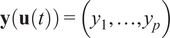 . The dynamics of these observables can be derived from the model of the system:

where
$ \mathrm{\mathcal{L}} $
 is linear and termed a Liouville operator. Defining the Liouville operator at
$ t={t}_0 $
is linear and termed a Liouville operator. Defining the Liouville operator at
$ t={t}_0 $
 yields
$ \mathrm{\mathcal{L}}\hskip0.1em \mathbf{y}={\nabla}_{{\mathbf{u}}_0}\mathbf{y}\left({\mathbf{u}}_0\right)\hskip0.24em \mathbf{f}\left({\mathbf{u}}_0\right) $
yields
$ \mathrm{\mathcal{L}}\hskip0.1em \mathbf{y}={\nabla}_{{\mathbf{u}}_0}\mathbf{y}\left({\mathbf{u}}_0\right)\hskip0.24em \mathbf{f}\left({\mathbf{u}}_0\right) $
 and the observables are then expressed as
$ \mathbf{y}\left(\mathbf{u}(t)\right)={e}^{\left(t-{t}_0\right)\mathrm{\mathcal{L}}}\hskip0.1em \mathbf{y}\left({\mathbf{u}}_0\right) $
and the observables are then expressed as
$ \mathbf{y}\left(\mathbf{u}(t)\right)={e}^{\left(t-{t}_0\right)\mathrm{\mathcal{L}}}\hskip0.1em \mathbf{y}\left({\mathbf{u}}_0\right) $
 .
.
Because the measurements are limited in number, the span
$ \mathcal{G}\hskip0.4em := \hskip0.4em \mathrm{span}\left({\left\{{y}_i\right\}}_i:\mathcal{S}\to \unicode{x211D}\right) $
 is finite, low-dimensional, and not invariant under the time-evolution operator governing the dynamics of
$ \mathbf{y}\left(\mathbf{u}\left(t>{t}_0\right)\right) $
is finite, low-dimensional, and not invariant under the time-evolution operator governing the dynamics of
$ \mathbf{y}\left(\mathbf{u}\left(t>{t}_0\right)\right) $
 . The dynamics of
$ \mathbf{y} $
. The dynamics of
$ \mathbf{y} $
 is then not closed in
$ \mathcal{G} $
is then not closed in
$ \mathcal{G} $
 , reflecting the fact that some information leaks in an orthogonal subspace
$ {\mathcal{G}}^{\perp } $
, reflecting the fact that some information leaks in an orthogonal subspace
$ {\mathcal{G}}^{\perp } $
 . To recover the missing information, it is necessary to describe how to express the dynamics of
$ \mathbf{y} $
. To recover the missing information, it is necessary to describe how to express the dynamics of
$ \mathbf{y} $
 not just as a function of itself, but also accounting for its history. The rationale is that the past values of
$ \mathbf{y} $
not just as a function of itself, but also accounting for its history. The rationale is that the past values of
$ \mathbf{y} $
 are influenced by unobserved quantities, or unresolved observables, of the system, not contained in
$ \mathcal{G} $
are influenced by unobserved quantities, or unresolved observables, of the system, not contained in
$ \mathcal{G} $
 . Carefully processing the history of these observables then allows us to account for the impact of the unresolved observables on the observables
$ \mathbf{y} $
. Carefully processing the history of these observables then allows us to account for the impact of the unresolved observables on the observables
$ \mathbf{y} $
 . A visual representation is presented in Figure 1.
Measuring the fully observed state of a system (left [1]) is often impossible due to its high dimensionality. Ultimately, the user only has, at their disposal, sparse observations of the full state that can be seen as a low-dimensional observable vector
$ \mathbf{y} $
 (middle [2]). The MZ equation DDE approximation (Proposition 2.1) can then be used to model partially observed systems (right [3]).
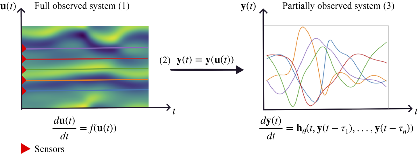
Figure 1. Long description
There are three panels arranged horizontally. The left panel is labeled Full observed system 1 and shows a heatmap with five horizontal red triangles labeled Sensors on the left edge. The vertical axis is labeled u of t and the horizontal axis is labeled t. Below, the equation d u of t over d t equals f of u of t is shown. The middle panel is a rightward arrow labeled 2 y of t equals y of u of t, indicating the mapping from the full system to observables. The right panel is labeled Partially observed system 3 and shows a line graph with five colored lines representing time series. The vertical axis is labeled y of t and the horizontal axis is labeled t. Below, the equation d y of t over d t equals h sub theta open parenthesis y of t, y of t minus tau sub 1, up to y of t minus tau sub n close parenthesis is shown.
2.1. The Mori–Zwanzig formalism
Different approaches leverage this past information. The Mori–Zwanzig (MZ) formalism, rooted in statistical physics, provides a framework to derive an evolution equation for a set of variables, such as macroscopic observables, associated with a high-dimensional dynamical system (Mori, Reference Mori1965; Zwanzig, Reference Zwanzig1966; Zwanzig et al., Reference Zwanzig, Nordholm and Mitchell1972). This framework is instrumental, for instance, in situations where the full state
$ \mathbf{u}(t) $
 is unavailable, and where one can only access low-dimensional observations. Similarly, the MZ formalism is also relevant for addressing dimension reduction problems (Zhu, Reference Zhu2019) where the reduced state is a set of variables whose dynamics are affected by the projected-out and nonobserved variables or state components.
In the Mori–Zwanzig framework, the span of
$ \mathcal{G} $
 of the measurements is considered as resulting from a projection through a projector
$ \mathcal{P} $
of the measurements is considered as resulting from a projection through a projector
$ \mathcal{P} $
 of the space of
$ {L}^2\left(\mathcal{S},\unicode{x211D}\right) $
of the space of
$ {L}^2\left(\mathcal{S},\unicode{x211D}\right) $
 functions. Similarly, the unobserved functions span a subspace resulting from a projection
$ \mathcal{Q} $
functions. Similarly, the unobserved functions span a subspace resulting from a projection
$ \mathcal{Q} $
 , with
$ \mathcal{Q}=\mathcal{I}-\mathcal{P} $
, with
$ \mathcal{Q}=\mathcal{I}-\mathcal{P} $
 . The dynamics of
$ \mathbf{y} $
. The dynamics of
$ \mathbf{y} $
 can then be expressed as

The influence of past unresolved dynamics on the current observations can be explicitly expressed using the Dyson identity, which states:

so that one can write the dynamics of the current observables
$ \mathbf{y}\left(\mathbf{u}(t)\right) $
 as:
as:

Rewriting Eq. (2.5) in a more compact form, and denoting
$ \mathbf{y}\left(\mathbf{u}(t)\right)=\mathbf{y}(t) $
 , the dynamics of the vector of observables
$ \mathbf{y}=(\hskip0.15em {y}_1,\dots, {y}_p) $
, the dynamics of the vector of observables
$ \mathbf{y}=(\hskip0.15em {y}_1,\dots, {y}_p) $
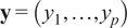 are shown to follow an integro-differential equation (IDE):

with
$ M $
 a Markovian operator and
$ K $
a Markovian operator and
$ K $
 an operator applied to past observables and integrated over the whole time span since the initial condition. The so-called “noise” term
$ F $
an operator applied to past observables and integrated over the whole time span since the initial condition. The so-called “noise” term
$ F $
 accounts for the impact of the unobserved variables at the initial condition. It can be eliminated from the equations predicting future observations by applying the projector
$ \mathcal{P} $
accounts for the impact of the unobserved variables at the initial condition. It can be eliminated from the equations predicting future observations by applying the projector
$ \mathcal{P} $
 and restricting their dynamics to the linear span of
$ \mathcal{P}\mathbf{y} $
and restricting their dynamics to the linear span of
$ \mathcal{P}\mathbf{y} $
 . Learning the dynamics of partially observed or known systems hence boils down to estimating each term of the differential equation above, sometimes referred to as the generalized Langevin equation (GLE).
Accounting for the past essentially allows us to isolate the dynamics of the observables. The Mori–Zwanzig framework is general and applies widely, allowing to describe the dynamics of the observables with a non-Markovian model. It similarly provides a principled closure for coarse models, hence missing information, which can be effectively complemented with a history-based term.
2.2. Approximations of integro-differential equations (IDE)
The statement in Eq. (2.6) outlines the structure of the dynamics. However, the operators involved in this dynamical equation are usually poorly known, if any, in particular the integral term. We now discuss several approaches from the literature to estimate these terms.
An approach to approximate the integral consists of studying particular asymptotic regimes. Among the many different models proposed in the literature (Stinis, Reference Stinis2004; Chorin and Stinis, Reference Chorin and Stinis2007; Stinis, Reference Stinis2007), one of the most popular consists in approximating the integral under assumptions of very short memory or very long memory regimes. For example, the t-model (Chorin et al., Reference Chorin, Hald and Kupferman2002), also commonly called slowly decaying memory approximation, leads to Markovian equations with time-dependent coefficients, which can subsequently be modeled using a NODE. However, these remain asymptotic approximations and cannot be extended to intermediate-range memory, in general. Another approach consists of performing Monte Carlo integration (Robert and Casella, Reference Robert and Casella1999). This approach has been extended to a neural network-based formulation (Neural IDE) (Zappala et al., Reference Zappala, de O. Fonseca, Moberly, Higley, Abdallah, Cardin and van Dijk2023), where the memory integrand is decomposed as a product
$ {K}_1\left(t,s\right)\hskip0.1em {K}_2\left(\mathbf{y}(s)\right) $
 . However, the number of function evaluations required to accurately integrate Equation (2.6) can be large, making the process computationally intensive (cf. Appendix A). In a similar spirit, under the assumption of short memory, one can restrict the integral to a short past and discretize it in time, leading to an equation of the form (Gallage, Reference Gallage2017):

using
$ n $
 delays
$ {\left\{{\tau}_i\right\}}_i $
delays
$ {\left\{{\tau}_i\right\}}_i $
 uniformly spaced over a past horizon instead of sampling them randomly. Such approximations can be improved using high-order discretization schemes, yet, as for Neural IDE, they require an unaffordable number of delays if the integrand varies quickly or if the time interval is too large.
2.3. Exact representation with neural DDE
While Equation (2.7) only provides an approximation of the true dynamics and requires many delays, we show that using a more complex function of a small number of delays, it is actually possible to represent the dynamics exactly. For this, let us consider diffeomorphic dynamical systems, that is, ODEs whose flow is invertible (in the full state space) and smooth in both time directions.
Proposition 2.1
(Exact representation with delays). For any smooth dynamical system (
$ {C}^2 $
 is enough), and differentiable observables
$ \mathbf{y} $
is enough), and differentiable observables
$ \mathbf{y} $
 , there exists almost surely an operator
$ M $
, there exists almost surely an operator
$ M $
 of the current observables, a finite number
$ n $
of the current observables, a finite number
$ n $
 of delays
$ {\tau}_1,\dots, {\tau}_n>0 $
of delays
$ {\tau}_1,\dots, {\tau}_n>0 $
 and a function
$ \mathbf{h} $
and a function
$ \mathbf{h} $
 such that the observables exactly follow the dynamics:

The derivation of the above, deferred to Appendix C, is based on the application of Takens’ theorem (hence the diffeomorphism requirement), which also provides a bound on the required number of delays: at least twice the intrinsic dimension of the manifold
$ \mathcal{S} $
 in which the full state
$ \mathbf{u} $
in which the full state
$ \mathbf{u} $
 lives. Note that this evolution equation is exact: approximations may arise from the optimization or the expressivity of the neural networks estimating
$ M $
lives. Note that this evolution equation is exact: approximations may arise from the optimization or the expressivity of the neural networks estimating
$ M $
 and
$ \mathbf{h} $
and
$ \mathbf{h} $
 , but not from the number of delays, provided they reach the Takens’ lower bound. This is in contrast with the discretization of the IDE integral as in Equation (2.7), which becomes asymptotically precise only when the number of delays is large compared to the complexity of the integrand.
3. Neural delay differential equations with learnable delays
The proposition 2.1 above motivates our approach. We consider learning the dynamics of the observables by accounting for their past in the form of a set of time-continuous coupled delayed differential equations (DDEs) involving a number of past observations
$ \left\{\mathbf{y}\left(t-{\tau}_1\right),\dots, \mathbf{y}\left(t-{\tau}_n\right)\right\} $
 . The vector field is approximated by a neural network and the resulting model is solved by NDDE, a neural differential equation solver dedicated to delayed equations (Monsel et al., Reference Monsel, Semeraro, Mathelin, Charpiat, Coelho, Zimmering, Costa, Ferrás and Niggemann2024). The Mori–Zwanzig framework provides a rigorous rationale, grounded in statistical physics, on how the dynamics of the observables are related to their past, involving a continuous integral over a past horizon. In contrast, the Takens’ theorem provides a geometrical view of the dynamics of a set of observables as a function of a sufficiently large number of delayed versions of themselves. These two frameworks motivate our approach of modeling the dynamics of the observables from a finite set of past observations via a learnable function. In addition, while the Takens’ theorem is not constructive when it comes to the value of the time lag, we here learn every individual delay
$ \left\{{\tau}_i\right\} $
. The vector field is approximated by a neural network and the resulting model is solved by NDDE, a neural differential equation solver dedicated to delayed equations (Monsel et al., Reference Monsel, Semeraro, Mathelin, Charpiat, Coelho, Zimmering, Costa, Ferrás and Niggemann2024). The Mori–Zwanzig framework provides a rigorous rationale, grounded in statistical physics, on how the dynamics of the observables are related to their past, involving a continuous integral over a past horizon. In contrast, the Takens’ theorem provides a geometrical view of the dynamics of a set of observables as a function of a sufficiently large number of delayed versions of themselves. These two frameworks motivate our approach of modeling the dynamics of the observables from a finite set of past observations via a learnable function. In addition, while the Takens’ theorem is not constructive when it comes to the value of the time lag, we here learn every individual delay
$ \left\{{\tau}_i\right\} $
 ,
$ 1\le i\le n $
,
$ 1\le i\le n $
 . The minimum number of delays
$ n $
. The minimum number of delays
$ n $
 is determined from the
$ {D}_2 $
is determined from the
$ {D}_2 $
 dimension of the underlying system, estimated from the dataset of observations.
3.1. Learning the delays
A constant lag NDDE is part of the larger family of continuous depth models that emerged with NODE (Chen et al., Reference Chen, Rubanova, Bettencourt, Duvenaud, Bengio, Wallach, Larochelle, Grauman, Cesa-Bianchi and Garnett2018). It is defined by:

with
$ \boldsymbol{\psi} $
 :
$ \unicode{x211D}\to {\unicode{x211D}}^m $
:
$ \unicode{x211D}\to {\unicode{x211D}}^m $
 the history function,
$ {\tau}_i\in {\unicode{x211D}}^{+} $
the history function,
$ {\tau}_i\in {\unicode{x211D}}^{+} $
 a delay constant and
$ {\mathbf{h}}_{\boldsymbol{\theta}}:\left[0,T\right]\times {\unicode{x211D}}^m\times \dots \times {\unicode{x211D}}^m\to {\unicode{x211D}}^m $
a delay constant and
$ {\mathbf{h}}_{\boldsymbol{\theta}}:\left[0,T\right]\times {\unicode{x211D}}^m\times \dots \times {\unicode{x211D}}^m\to {\unicode{x211D}}^m $
 a neural network.
There are two possible ways of training continuous-depth models: discretize-then-optimize or optimize-then-discretize (Kidger, Reference Kidger2021). In the former, the numerical simulation library’s inherent auto-differentiation capabilities are leveraged. In the latter, the adjoint dynamics are employed to compute the gradient’s loss. The following proposition 3.1 provides the adjoint method for constant lag NDDEs.
Proposition 3.1. Let us consider the Neural DDE model below, where
$ \tau $
 is a learnable vector parameterized by some components of
$ \boldsymbol{\theta} $
is a learnable vector parameterized by some components of
$ \boldsymbol{\theta} $
 :
:

and the following loss function:
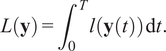
The gradient of the loss with respect to the parameters is given by:

where
$ {\mathbf{y}}_{\left(\tau \right)}(t)\equiv \mathbf{y}\left(t-\tau \right) $
 is the third set of variables
$ {\mathbf{h}}_{\boldsymbol{\theta}}\left(t,\mathbf{y},{\mathbf{y}}_{\left(\tau \right)}\right) $
is the third set of variables
$ {\mathbf{h}}_{\boldsymbol{\theta}}\left(t,\mathbf{y},{\mathbf{y}}_{\left(\tau \right)}\right) $
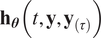 depends on. The adjoint dynamics
$ \boldsymbol{\lambda} (t) $
depends on. The adjoint dynamics
$ \boldsymbol{\lambda} (t) $
 are given by another DDE:

The derivation of Proposition 3.1 is in Appendix B. Algorithm 1 below outlines the training procedure for a Neural DDE with multiple learnable constant delays, defined for convenience as
$ {\mathbf{y}}_{\left({\tau}_i\right)}(t)=\mathbf{y}\left(t-{\tau}_i\right) $
 .
.
The developments are packaged in a user-friendly API, developing a numerically robust DDE solver, and implementing the adjoint method in the torchdde package. These advancements allow a seamless integration of DDEs for future users, enhancing reproducibility. Computational details and benchmarks are reported in Appendix A.2.
Algorithm 1 Training a Neural DDE with learnable delays with the adjoint method.
Require: Dataset of one trajectory
$ \mathcal{D}=\left\{\left({t}_0,{\mathbf{y}}_0\right),\dots, \left({t}_T,{\mathbf{y}}_T\right)\right\}. $

Require: Initialized model
$ {\mathbf{h}}_{\boldsymbol{\theta}}. $

Require: Initialized positive delays
$ {\tau}_1,\dots, {\tau}_n $
 , handled as additional entries in the parameters vector
$ \boldsymbol{\theta} $
, handled as additional entries in the parameters vector
$ \boldsymbol{\theta} $
 .
.
1: for
$ {N}_{\mathrm{epochs}} $
 do
do
2: Set
$ {\tau}_{\mathrm{max}}=\max \left\{{\tau}_1,\dots, {\tau}_n\right\} $

3: Create history function interpolation
$ \psi $
 with data from
$ \mathcal{D} $
with data from
$ \mathcal{D} $
 such that
$ t\le {t}_0+{\tau}_{\mathrm{max}} $
such that
$ t\le {t}_0+{\tau}_{\mathrm{max}} $
 .
.
4: Solve DDE dynamics:
5:
$ \left\{\begin{array}{l}{\displaystyle \frac{\mathrm{d}\mathbf{y}(t)}{\mathrm{d}t}}={\mathbf{h}}_{\boldsymbol{\theta}}(t,\mathbf{y}(t),{\mathbf{y}}_{({\tau}_1)}(t),\dots, {\mathbf{y}}_{({\tau}_n)}(t))\\ {}\mathbf{y}(t\le {t}_0+{\tau}_{\mathrm{max}})=\boldsymbol{\psi} (t)\end{array}\right.\operatorname{}\hskip0.1em $
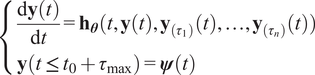
6: Compute loss
$ L\left(\mathbf{y}\right)={\int}_{t_0+{\tau}_{\mathrm{max}}}^{t_T}l\left(\mathbf{y}(t)\right)\hskip0.1em \mathrm{d}t $

7: Solve Adjoint dynamics:
8:
$ \left\{\begin{array}{l}\dot{\boldsymbol{\lambda}}(t)={\displaystyle \frac{\mathrm{\partial}l(\mathbf{y}(t))}{\mathrm{\partial}\mathbf{y}}}-\boldsymbol{\lambda} (t){\displaystyle \frac{\mathrm{\partial}{\mathbf{h}}_{\boldsymbol{\theta}}(t,\mathbf{y}(t),{\mathbf{y}}_{({\tau}_1)}(t),\dots, {\mathbf{y}}_{({\tau}_n)}(t))}{\mathrm{\partial}\mathbf{y}}}\\ {}\hskip1.9pc -\sum \limits_{i=1}^n\boldsymbol{\lambda} (t+{\tau}_i){\displaystyle \frac{\mathrm{\partial}{\mathbf{h}}_{\boldsymbol{\theta}}(t+{\tau}_i,\mathbf{y}(t+{\tau}_i),{\mathbf{y}}_{({\tau}_1)}(t+{\tau}_i),\dots, {\mathbf{y}}_{({\tau}_n)}(t+{\tau}_i))}{\mathrm{\partial}{\mathbf{y}}_{({\tau}_i)}}}\\ {}\boldsymbol{\lambda} (t\ge {t}_T)=\mathbf{0}.\end{array}\right.\operatorname{}\hskip0.1em $
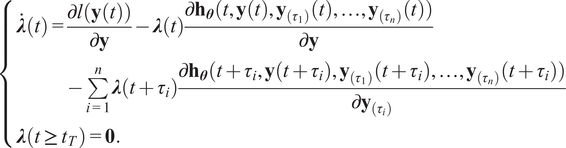
9: Compute
$ \frac{\partial L}{\partial \boldsymbol{\theta}} $
 :
:
10:

11: Update
$ \boldsymbol{\theta} $

12: end for
3.2. On the importance of relevant delays
Learning the delays
$ {\tau}_i $
 within NDDEs is crucial for accurately modeling partially observed dynamics, and therefore, delays need to be adapted during training. To illustrate the impact of the relevant delays, we evaluate the information that past observations share with the current dynamics of the observable, and how this varies with the delay. To this end, let us consider a dynamical system evolving on a compact smooth manifold
$ \mathcal{S}\subset {\unicode{x211D}}^m $
within NDDEs is crucial for accurately modeling partially observed dynamics, and therefore, delays need to be adapted during training. To illustrate the impact of the relevant delays, we evaluate the information that past observations share with the current dynamics of the observable, and how this varies with the delay. To this end, let us consider a dynamical system evolving on a compact smooth manifold
$ \mathcal{S}\subset {\unicode{x211D}}^m $
 described by a simple 2-delay dynamical system, assumed to be an attractor, and let us consider a
$ {C}^2 $
described by a simple 2-delay dynamical system, assumed to be an attractor, and let us consider a
$ {C}^2 $
 observable function
$ y:\mathcal{S}\to \unicode{x211D} $
observable function
$ y:\mathcal{S}\to \unicode{x211D} $


with
$ \alpha =0.2 $
 ,
$ {\tau}_1={p}_1^{\star}\hskip0.1em \Delta t $
,
$ {\tau}_1={p}_1^{\star}\hskip0.1em \Delta t $
 ,
$ {\tau}_2={p}_2^{\star}\hskip0.1em \Delta t $
,
$ {\tau}_2={p}_2^{\star}\hskip0.1em \Delta t $
 ,
$ {p}_1^{\star }=250 $
,
$ {p}_1^{\star }=250 $
 ,
$ {p}_2^{\star }=400 $
,
$ {p}_2^{\star }=400 $
 and
$ \operatorname{sinc}(x):= \sin (x)/x $
and
$ \operatorname{sinc}(x):= \sin (x)/x $
 for
$ x\ne 0 $
for
$ x\ne 0 $
 ,
$ \operatorname{sinc}(0) $
,
$ \operatorname{sinc}(0) $
 := 1.
:= 1.
The Takens’ theorem (Takens, Reference Takens, Rand and Young1981) rigorously discusses the conditions under which a delayed vector of real-valued observables
$ \left(y\left(\mathbf{u}(t)\right),y\left(\mathbf{u}\left(t-\tau \right)\right),\dots, y\left(\mathbf{u}\left(t- n\tau \right)\right)\right) $
 ,
$ n\in \unicode{x2115} $
,
$ n\in \unicode{x2115} $
 , defines an embedding, a smooth diffeomorphism onto its image. It guarantees a topological equivalence between the original dynamical system and the one constructed from the memory of the observable. The dynamics of the system can then be reformulated on the set
$ \left(y\left(\mathbf{u}(t)\right),y\left(\mathbf{u}\left(t-\tau \right)\right),\dots, y\left(\mathbf{u}\left(t- n\tau \right)\right)\right) $
, defines an embedding, a smooth diffeomorphism onto its image. It guarantees a topological equivalence between the original dynamical system and the one constructed from the memory of the observable. The dynamics of the system can then be reformulated on the set
$ \left(y\left(\mathbf{u}(t)\right),y\left(\mathbf{u}\left(t-\tau \right)\right),\dots, y\left(\mathbf{u}\left(t- n\tau \right)\right)\right) $
 . However, Takens’ theorem, later extended by Sauer et al. (Reference Sauer, Yorke and Casdagli1991), provides a sufficient condition for reconstruction, but does not specify how to choose the time delay
$ \tau $
. However, Takens’ theorem, later extended by Sauer et al. (Reference Sauer, Yorke and Casdagli1991), provides a sufficient condition for reconstruction, but does not specify how to choose the time delay
$ \tau $
 . From a mathematical viewpoint, the delay could be arbitrary, besides some specific values excluded by the theorem. In practice, its value can strongly condition a successful embedding. If too small, entries of the delay vector data are too similar; if too large, the entries tend to be completely uncorrelated and cannot be numerically linked to a consistent dynamical system (Kantz and Schreiber, Reference Kantz and Schreiber2003).
We here illustrate the impact of suitable delays on the relevance of the information available to inform the future evolution of the observable. The relevance of the delays
$ \left\{{\tau}_1,{\tau}_2\right\} $
 for informing
$ y\left(t+\Delta t\right) $
for informing
$ y\left(t+\Delta t\right) $
 is assessed in terms of the mutual information between
$ \left(y\left(t-{\tau}_1\right),y\left(t-{\tau}_2\right)\right) $
is assessed in terms of the mutual information between
$ \left(y\left(t-{\tau}_1\right),y\left(t-{\tau}_2\right)\right) $
 and
$ y(t) $
and
$ y(t) $
 , as suggested in Frase and Swinney (Reference Fraser and Swinney1986). The mutual information
$ I\left(X,Y\right) $
, as suggested in Frase and Swinney (Reference Fraser and Swinney1986). The mutual information
$ I\left(X,Y\right) $
 between two random variables
$ X $
between two random variables
$ X $
 and
$ Y $
and
$ Y $
 quantifies the amount of information observing a variable brings about the other one. By considering the problem in Equation (3.5), we estimate the information shared between the current observations
$ y(t) $
quantifies the amount of information observing a variable brings about the other one. By considering the problem in Equation (3.5), we estimate the information shared between the current observations
$ y(t) $
 and their past values
$ y\left(t-{\tau}_1\right) $
and their past values
$ y\left(t-{\tau}_1\right) $
 ,
$ y\left(t-{\tau}_2\right) $
,
$ y\left(t-{\tau}_2\right) $
 and is shown in Figure 2 as a 2-D map in terms of
$ {p}_1 $
and is shown in Figure 2 as a 2-D map in terms of
$ {p}_1 $
 and
$ {p}_2 $
and
$ {p}_2 $
 . The map is symmetric, as expected since
$ I\left(\left(y\left(t-{\tau}_1\right),y\left(t-{\tau}_2\right)\right),y(t)\right)=I\left(\left(y\left(t-{\tau}_2\right),y\left(t-{\tau}_1\right)\right),y(t)\right) $
. The map is symmetric, as expected since
$ I\left(\left(y\left(t-{\tau}_1\right),y\left(t-{\tau}_2\right)\right),y(t)\right)=I\left(\left(y\left(t-{\tau}_2\right),y\left(t-{\tau}_1\right)\right),y(t)\right) $
 . It can be seen that the amount of information shared between the current observation and a delay vector of the observable significantly varies with the delays and indeed reaches a maximum for
$ {\tau}_1={p}_1^{\star}\hskip0.1em \Delta t $
. It can be seen that the amount of information shared between the current observation and a delay vector of the observable significantly varies with the delays and indeed reaches a maximum for
$ {\tau}_1={p}_1^{\star}\hskip0.1em \Delta t $
 ,
$ {\tau}_2={p}_2^{\star}\hskip0.1em \Delta t $
,
$ {\tau}_2={p}_2^{\star}\hskip0.1em \Delta t $
 . The ability of the present Neural DDE method to learn the delays, in addition to the model
$ {\mathbf{h}}_{\boldsymbol{\theta}} $
. The ability of the present Neural DDE method to learn the delays, in addition to the model
$ {\mathbf{h}}_{\boldsymbol{\theta}} $
 , is thus key to its performance and wide applicability.
$ \left\{{\tau}_1={p}_1\hskip0.1em \Delta t,{\tau}_2={p}_2\hskip0.1em \Delta t\right\} $
 -map of delayed mutual information,
$ I\left(\left(y\left(t-{\tau}_1\right),y\left(t-{\tau}_2\right)\right),y(t)\right) $
-map of delayed mutual information,
$ I\left(\left(y\left(t-{\tau}_1\right),y\left(t-{\tau}_2\right)\right),y(t)\right) $
 . The maximum is exhibited at
$ \left({p}_1,{p}_2\right) $
. The maximum is exhibited at
$ \left({p}_1,{p}_2\right) $
 =
$ \left(250,400\right) $
=
$ \left(250,400\right) $
 and
$ \left(\mathrm{400,250}\right) $
and
$ \left(\mathrm{400,250}\right) $
 , in agreement with
$ {p}_1^{\star }=250 $
, in agreement with
$ {p}_1^{\star }=250 $
 ,
$ {p}_2^{\star }=400 $
,
$ {p}_2^{\star }=400 $
 .
.
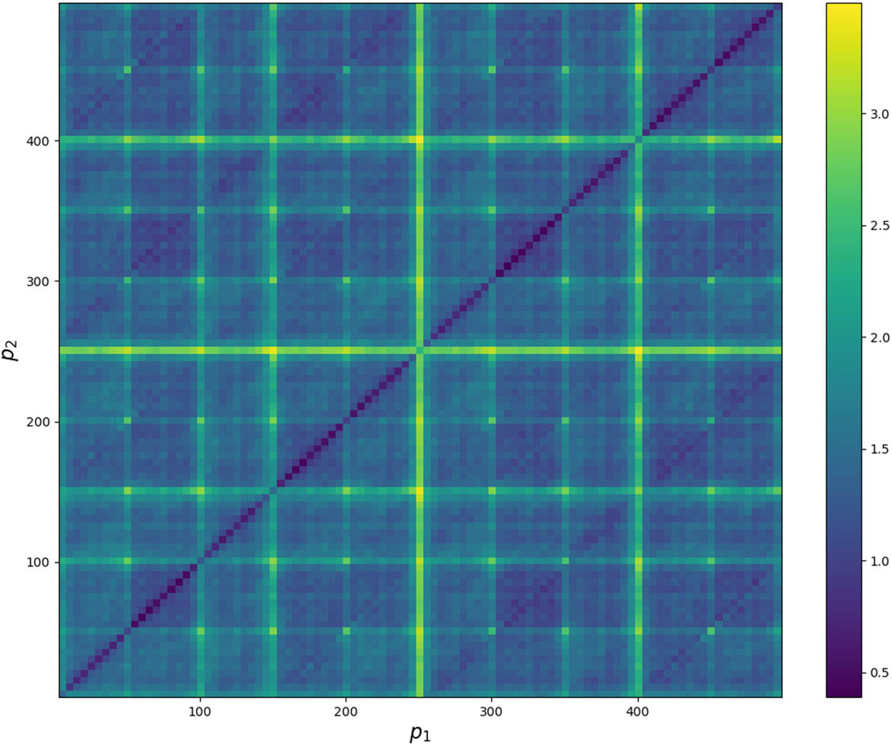
Figure 2. Long description
The heatmap plots p one on the horizontal axis and p two on the vertical axis, both ranging from zero to four hundred fifty. Color intensity represents the value of delayed mutual information, with the scale bar on the far right ranging from zero point five (dark purple) to above three point zero (yellow). A prominent diagonal of high values runs from the bottom left to the top right, indicating symmetry. Brightest maxima are observed at coordinates two hundred fifty, four hundred and four hundred, two hundred fifty, as well as at regular intervals along both axes, forming a grid-like pattern. The axes are labeled in italic font as p one (horizontal) and p two (vertical). The color bar is labeled with values increasing from bottom to top.
4. Experiments
We now demonstrate the present approach and its capability to jointly learn the delays in addition to a model of the dynamics. Several experiments are considered, ranging from synthetic low-dimensional dynamical systems to time-series predictions in an experimental configuration. In addition to accurately learning the dynamics, the relevance of being able to learn suitable delays is also demonstrated.
4.1. Dynamical systems
In the following, the dynamical systems considered in this article are presented. All datasets are divided into training, validation, and test sets with proportions of 70%, 10%, and 20%, respectively, and the Dormand–Prince (Dopri5) solver was used for data generation and training (Dormand and Prince, Reference Dormand and Prince1980). Table 1 outlines the number of delays employed in NDDE for each experiment.
Number of delays used in NDDE for each experiment

Table 1. Long description
The table contains one header row and one data row. The header row lists three experiments from left to right: KS, Cavity, and Brusselator. The single data row is labeled NDDE at the far left. The NDDE values for each experiment are as follows: KS is 5, Cavity is 1, and Brusselator is 2. All values are centered within their respective columns.
4.1.1. Population dynamics model
As a first example, we consider the dynamics of a scalar-valued system used to model population dynamics in biology (Arino et al., Reference Arino, Hbid and Dads2009; Banks et al., Reference Banks, Banks, Bommarco, Laubmeier, Myers, Rundlöf and Tillman2017). Such a system is formulated through the following DDE:

where we integrate from
$ t\in \left[0,10\right] $
 ,
$ \tau =1 $
,
$ \tau =1 $
 ,
$ \psi (t)={u}_0 $
,
$ \psi (t)={u}_0 $
 ,
$ {u}_0 $
,
$ {u}_0 $
 is sampled from the uniform distribution
$ \mathcal{U}\left(\mathrm{2.0,3.0}\right) $
is sampled from the uniform distribution
$ \mathcal{U}\left(\mathrm{2.0,3.0}\right) $
 and
$ 256 $
and
$ 256 $
 trajectories were generated.
4.1.2. Brusselator
A second experiment showcases how NDDEs can effectively model partially observed systems with past state values. We consider the 2-species Belousov–Zhabotinsky kinetic equation (Belousov, Reference Belousov1959; Zhabotinskii, Reference Zhabotinskii1964) that can be modeled by the so-called Brusselator system:

with
$ {u}_1(t) $
 and
$ {u}_2(t) $
and
$ {u}_2(t) $
 the two species concentrations at a given time. We integrate in the time domain
$ t\in \left[0,25\right] $
the two species concentrations at a given time. We integrate in the time domain
$ t\in \left[0,25\right] $
 . The initial condition
$ {u}_1 $
. The initial condition
$ {u}_1 $
 is sampled from the uniform distribution
$ \mathcal{U}\left(\mathrm{0,2.0}\right) $
is sampled from the uniform distribution
$ \mathcal{U}\left(\mathrm{0,2.0}\right) $
 while
$ {u}_2=0.0 $
while
$ {u}_2=0.0 $
 and
$ 1024 $
and
$ 1024 $
 trajectories were generated. We set ourselves in the partially observable case, where we only have access to the dynamics of
$ {u}_1 $
trajectories were generated. We set ourselves in the partially observable case, where we only have access to the dynamics of
$ {u}_1 $
 , that is,
$ y(t)\equiv {u}_1(t) $
, that is,
$ y(t)\equiv {u}_1(t) $
 , and wish to reconstruct the whole dynamics.
4.1.3. Kuramoto–Sivashinsky (KS) system
This model was originally derived to describe the complex dynamics of flames in a combustion. The Kuramoto–Sivashinsky system is described as:

The system is integrated over the time domain
$ t\in \left[0,30\right] $
 and its spatial domain
$ {D}_x=\left[0,22\right] $
and its spatial domain
$ {D}_x=\left[0,22\right] $
 is discretized into 128 points. A total of
$ 2048 $
is discretized into 128 points. A total of
$ 2048 $
 trajectories were generated from the initial condition samples. To put ourselves in the partially observed setting, we choose to observe the solution in time at
$ p $
trajectories were generated from the initial condition samples. To put ourselves in the partially observed setting, we choose to observe the solution in time at
$ p $
 locations uniformly spread across the spatial domain (we retain
$ p=5 $
locations uniformly spread across the spatial domain (we retain
$ p=5 $
 ).
).
4.1.4. Incompressible open cavity flow
As an experimental demonstrator, we consider the modeling based on time-series derived from wind tunnel experiments of an open cavity flow sketched in Figure 3. The facility and the details of the experimental setup are described in Tuerke et al. (Reference Tuerke, Lusseyran, Sciamarella, Pastur and Artana2020). Open cavity flows have attracted numerous research efforts in the last few decades due to the interesting dynamics at work. The flow is characterized by an impinging shear layer activating a centrifugal instability in a cavity. This interplay, reminiscent of the feedback acoustic mechanisms described in Rossiter (Reference Rossiter1964)), leads to a self-sustained oscillation. A broad range of dynamics is observed, ranging from limit cycles to toroidal and chaotic dynamics. The system is observed through a sensor in
$ P $
 measuring the local pressure fluctuations, hence
$ y(t)\equiv P\left(t;{\mathbf{x}}_{\mathrm{P}}\right) $
measuring the local pressure fluctuations, hence
$ y(t)\equiv P\left(t;{\mathbf{x}}_{\mathrm{P}}\right) $
 . The data are obtained for a Reynolds number
$ \mathit{\operatorname{Re}}=9190 $
. The data are obtained for a Reynolds number
$ \mathit{\operatorname{Re}}=9190 $
 based on the length L of the cavity.
Sketch of open cavity flow taken from (Tuerke et al., Reference Tuerke, Lusseyran, Sciamarella, Pastur and Artana2020). A data-acquiring sensor is placed in P. The cavity has a length L and depth H. The incoming laminar boundary layer flow is characterized by the freestream velocity
$ {U}_{\infty } $
 and the momentum thickness
$ {\Theta}_0 $
and the momentum thickness
$ {\Theta}_0 $
 .
.
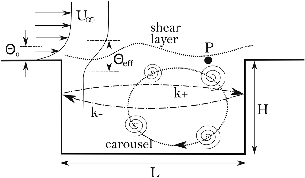
Figure 3. Long description
At the left, horizontal arrows indicate incoming laminar flow with freestream velocity U sub infinity and initial momentum thickness Theta sub 0. The flow enters a rectangular cavity, with the top edge labeled Theta sub effective. Above the cavity, a dashed line marks the shear layer, and a filled circle labeled P denotes the sensor position. Inside the cavity, two large counter-rotating vortices are shown by spiral arrows, labeled k plus and k minus, forming a carousel pattern. The cavity’s horizontal length is labeled L and vertical depth H. All labels are positioned relative to the cavity geometry, with flow direction indicated by arrows.
4.2. Results
We now assess the performance of the models with their ability to predict future measurements of a partially observed system. In this study, LSTM, NODE, ANODE, Latent ODE, and NDDE were selected for comparison. Table 2 displays the test MSE loss over each experiment. Appendix D goes into more detail about each model’s architecture and the training and testing procedure. Every model incorporates a form of “memory” into its architecture, with the exception of NODE. While LSTM and Latent ODE utilize hidden units and ANODE employs its augmented state
$ \mathbf{a}(t) $
 , NDDE leverages past observations such as
$ \mathbf{y}\left(t-\tau \right) $
, NDDE leverages past observations such as
$ \mathbf{y}\left(t-\tau \right) $
 . In all subsequent figures, the y-axis
$ \mathbf{y}(t) $
. In all subsequent figures, the y-axis
$ \mathbf{y}(t) $
 represents our observables (introduced for each system in Section 4.1), defined as
$ \mathbf{y}(t)=y\left(\mathbf{u}(t)\right) $
represents our observables (introduced for each system in Section 4.1), defined as
$ \mathbf{y}(t)=y\left(\mathbf{u}(t)\right) $
 .
.
Model performance (MSE) over the test set in each experiment averaged over five runs

Table 2. Long description
The table has three rows for experiments: Brusselator, K S, and Cavity. Each row lists mean squared error values plus or minus standard deviation for five models. For Brusselator: L S T M is 0.0051 plus or minus 0.0031, N O D E is 0.77 plus or minus 0.00080, A N O D E is 0.0050 plus or minus 0.0050, Latent O D E is 0.014 plus or minus 0.0076, N D D E is 0.016 plus or minus 0.0076. For K S: L S T M is 0.77 plus or minus 0.041, N O D E is 0.71 plus or minus 0.10, A N O D E is 0.55 plus or minus 0.027, Latent O D E is 0.43 plus or minus 0.07, N D D E is 0.28 plus or minus 0.024. For Cavity: L S T M is 0.75 plus or minus 0.46, N O D E is 0.96 plus or minus 0.0011, A N O D E is 0.65 plus or minus 0.0090, Latent O D E is 0.25 plus or minus 0.14, N D D E is 0.13 plus or minus 0.012. Lower values indicate better performance, with N D D E generally showing the lowest errors for K S and Cavity, and A N O D E and L S T M performing best for Brusselator.
4.2.1. Population dynamics model
Figures 4 and 5, respectively, depict the model’s robust convergence to accurate dynamics and the evolution of the delay
$ \tau $
 during training over many seeds, showcasing a consequence of Takens’ theorem (Takens, Reference Takens, Rand and Young1981). Using a delay-coordinate map, one can indeed construct a diffeomorphic shadow manifold
$ {M}^{\prime } $
during training over many seeds, showcasing a consequence of Takens’ theorem (Takens, Reference Takens, Rand and Young1981). Using a delay-coordinate map, one can indeed construct a diffeomorphic shadow manifold
$ {M}^{\prime } $
 from univariate observations of the original system in the generic sense. We here observe the whole state, so that
$ y(t)\equiv u(t) $
from univariate observations of the original system in the generic sense. We here observe the whole state, so that
$ y(t)\equiv u(t) $
 , and the delay coordinate map is then in terms of
$ \left(y(t),y\left(t-\tau \right)\right) $
, and the delay coordinate map is then in terms of
$ \left(y(t),y\left(t-\tau \right)\right) $
 , with
$ \tau >0 $
, with
$ \tau >0 $
 . The result of Figure 5 shows that the learned delay can lie between about 0.8 and 1.4. In classical approaches (see Tan et al. (Reference Tan, Algar, Corrêa, Small, Stemler and Walker2023), the selected delay with Takens’ theorem for State Space Reconstruction is typically chosen close to the minimum delayed mutual information of the time series.
The prediction of the DDE model is seen to accurately match the true evolution.
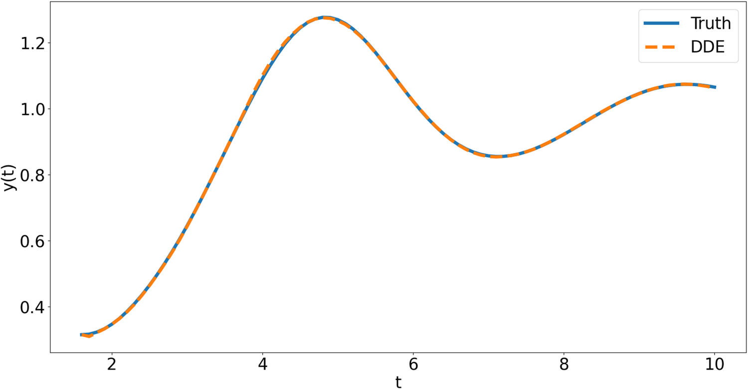
Toy dataset delay evolution during training for several initial conditions.
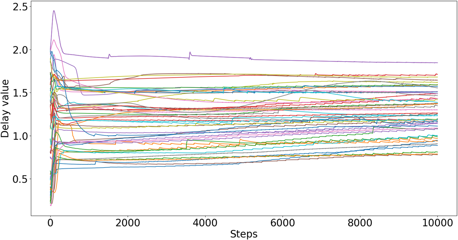
Figure 5. Long description
The x axis is labeled Steps, ranging from 0 to 10,000. The y axis is labeled Delay value, spanning 0.5 to 2.5. Multiple colored lines begin at the left edge, each representing a distinct initial condition. Most lines start with rapid changes, then stabilize horizontally between delay values of 0.5 and 2.0 as steps increase. A few lines show higher initial spikes above 2.0 before settling. The majority of trajectories converge to steady values, with minor fluctuations visible throughout. No legend or specific line labels are present.
4.2.2. Brusselator
In the case of this stiff and periodic dynamics, all models demonstrate satisfactory performance except NODE, which essentially predicts a mean trajectory thus highlighting the importance of incorporating memory terms for an accurate prediction. Remarkably, both LSTM and ANODE perform equally well, with NDDE and Latent ODE slightly trailing by a narrow margin as shown in Figure 6. In addition to evaluating the MSE loss performance, Figure 7 demonstrates the stability of each trained model on the Brusselator system over an extended period. After training within a specific time interval, we lengthened the integration period to five times the original training duration to assess the models’ performance. It is observed that NDDE, along with LSTM, NODE, and Latent ODE, are the only models that remain stable throughout this duration, with NDDE exhibiting the best performance over the extended horizon.
Examples of prediction of the Brusselator dynamics in terms of
$ y(t)\equiv {u}_1(t) $
 , for initial conditions sampled at random.
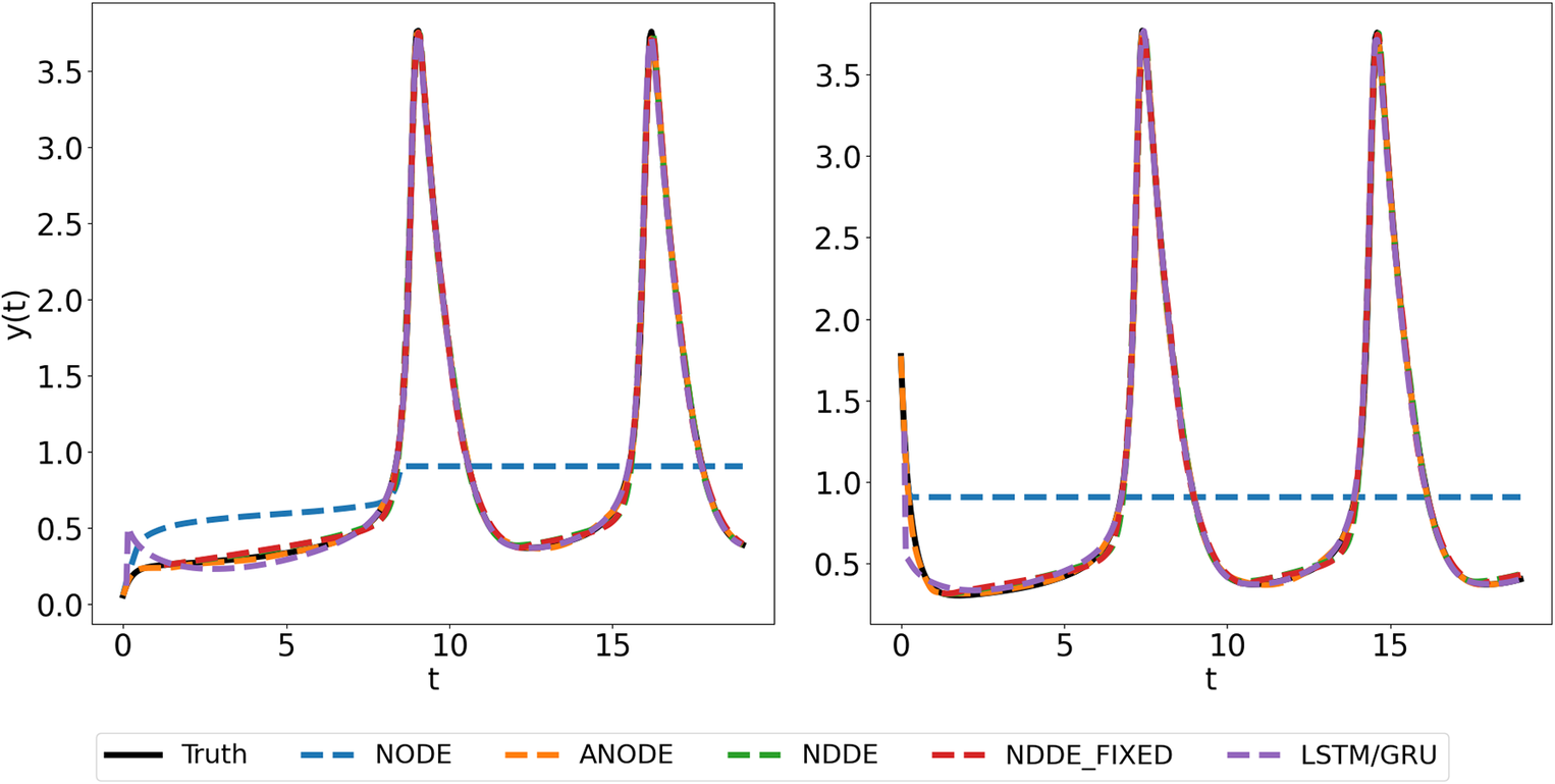
Figure 6. Long description
The left panel shows y of t on the vertical axis from 0 to 4 and t on the horizontal axis from 0 to 20. Six lines are plotted: Truth (solid black), NODE (blue dashed), ANODE (orange dashed), NDDE (red dashed), NDDE_FIXED (green dashed), and LSTM forward slash G R U (purple dashed). The Truth, ANODE, NDDE, NDDE_FIXED, and LSTM forward slash G R U lines overlap, showing sharp periodic peaks at t near 10 and 17. The NODE line deviates, remaining nearly flat at y of t equals 1. The right panel repeats the same axes and legend. All models except NODE closely follow the Truth, with three sharp peaks at similar t values. The NODE line remains flat. The legend below the panels identifies each line style and color.
Phase-portrait of
$ \left(y(t),\dot{y}(t)\right) $
 . Long-term behavior of each trained model for the Brusselator system.
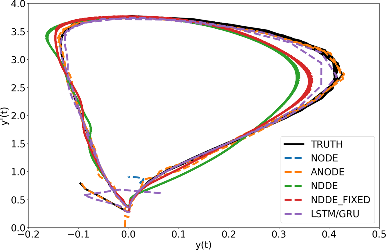
Figure 7. Long description
The x axis is labeled y of t, ranging from negative zero point two to zero point five. The y axis is labeled y dot of t, ranging from zero to four. Six trajectories are plotted: TRUTH in solid black, NODE in dashed blue, ANODE in dashed orange, NDDE in solid green, NDDE FIXED in dashed red, and LSTM forward slash G R U in dashed purple. All trajectories form closed loops with similar shapes but show visible deviations, especially near the lower left and upper right regions. The TRUTH trajectory is the reference, with other models approximating it to varying degrees. The legend is located in the lower right quadrant.
4.2.3. KS system
This numerical experiment deals with a partially observed system in a chaotic regime, observed through the solution at
$ p $
 locations uniformly spread across the spatial domain. Figure 8 showcases random test samples from two different initial conditions, highlighting how NDDEs outperform other models struggling with the dynamics of the selected features. In a chaotic setting, the statistics of the dynamics are often more informative than the trajectory itself. We hence focus on the probability distribution of the prediction across a large time horizon for the different
$ p $
locations uniformly spread across the spatial domain. Figure 8 showcases random test samples from two different initial conditions, highlighting how NDDEs outperform other models struggling with the dynamics of the selected features. In a chaotic setting, the statistics of the dynamics are often more informative than the trajectory itself. We hence focus on the probability distribution of the prediction across a large time horizon for the different
$ p $
 components of the observables
$ {\left\{{y}_i\right\}}_{i=1}^p $
components of the observables
$ {\left\{{y}_i\right\}}_{i=1}^p $
 , cf. Figure 9. It is seen that NDDE again outperforms the other approaches, with predictions that are statistically closer to the ground truth. This is further supported by the evolution of the maximum Lyapunov exponent (MLE) of the resulting models. Table 3 displays the MLE estimates for each model, showing that the Neural DDE with learnable delays closely aligns with the ground truth compared to other models.
Prediction of the KS system from a test sample for different models.
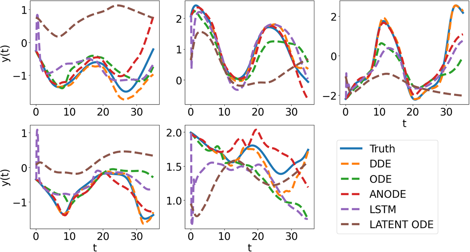
Figure 8. Long description
Starting from the top-left panel and proceeding rightward, each graph plots y of t versus t for a test sample. The x-axis is labeled t, ranging from 0 to about 35. The y-axis is labeled y of t, with varying ranges per panel. Each panel overlays six colored lines: solid blue for Truth, dashed orange for D D E, dashed green for O D E, dashed red for A N O D E, dashed purple for L S T M, and dashed brown for Latent O D E. The legend in the bottom right specifies these mappings. Across panels, the Truth line shows oscillatory behavior, while model predictions diverge in amplitude and phase, with Latent O D E often deviating most. The panels illustrate differences in model accuracy and dynamics for the KS system.
Probability density functions of the predictions
$ {y}_i(t) $
 over the time horizon and across several initial conditions for different models. KS system.
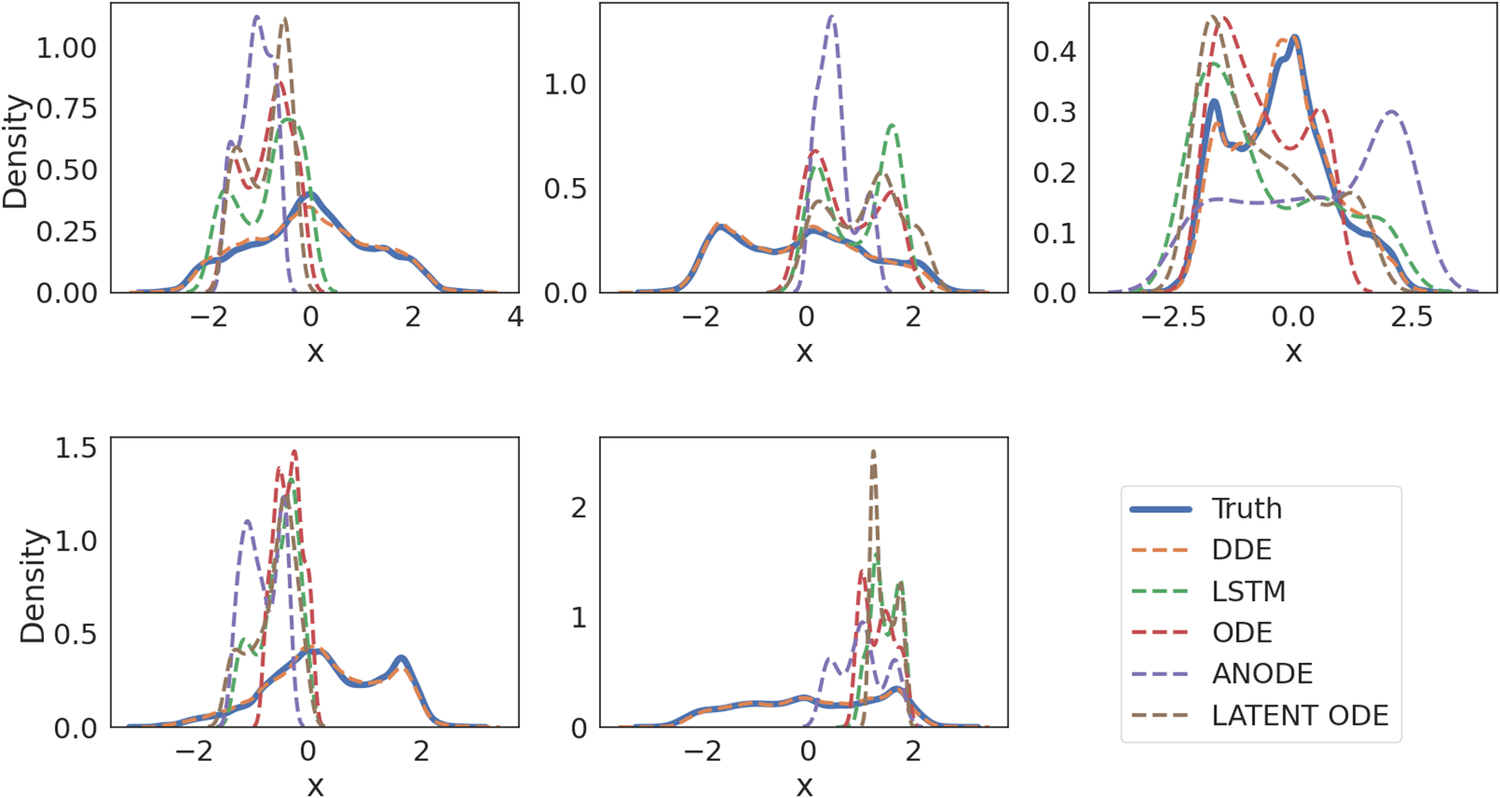
Figure 9. Long description
Starting at the top left and moving right, then to the bottom row, each panel shows density on the y axis and X on the x axis. Six lines are plotted per panel: solid blue for Truth, dashed orange for D D E, dashed green for L S T M, dashed red for O D E, dashed purple for A N O D E, and dashed brown for Latent O D E. The legend is in the bottom right panel. Each panel displays different distributions, with the Truth line generally smoother and the model lines showing varying degrees of deviation and multimodality. Peaks and spread differ by panel, reflecting changes in initial conditions. Some models, such as A N O D E and Latent O D E, show sharper or shifted peaks compared to Truth. The density range and x axis limits vary slightly between panels, highlighting the diversity of prediction behaviors across models and conditions.
Estimation of the maximum Lyapunov exponent
$ {\boldsymbol{\lambda}}_{\mathrm{max}} $
 for the KS system based on the generated trajectories from the test set for each model

Table 3. Long description
Column headers from left to right are Ground truth, N D D E, N O D E, A N O D E, and Latent O D E. The row label is lambda sub max. Ground truth is 0.129, N D D E is 0.128, N O D E is 0.097, A N O D E is 0.120, Latent O D E is 0.035. N D D E is bolded, indicating it is closest to ground truth. Latent O D E is the lowest value. The table compares the estimation of the maximum Lyapunov exponent for the KS system based on generated trajectories from the test set for each model.
4.2.4. Cavity
In this experimental fluid flow configuration, the NDDE formulation again outperforms other models, as illustrated in Figure 10 where the predictions are plotted for two test samples. The benefit of a time-delay model here comes from the fact that this experimental setup involves a large vortex within the cavity, effectively acting like a feedback loop and hence suitably described by governing equations involving delayed contributions. Latent ODE yields acceptable results compared to NODE, which only generates the system’s average trajectory, while LSTM and ANODE capture oscillations, albeit occasionally in conflicting phases. These experiments demonstrate that NDDE can effectively model trajectories even in the presence of noise in the data, such as in this experimental dataset.
Prediction of the cavity observables from different models for two test samples.
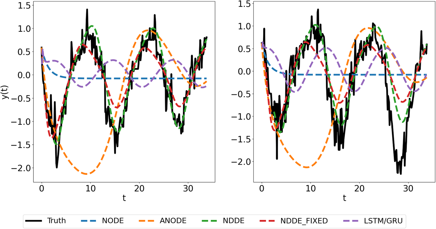
Figure 10. Long description
The left panel shows y of t versus t from 0 to about 33. The black solid line labeled Truth shows the reference data with sharp oscillations. The blue dashed line labeled N O D E remains near zero. The orange dashed line labeled A N O D E shows a large amplitude oscillation out of phase with Truth. The green dashed line labeled N D D E and the red dashed line labeled N D D E underscore F I X E D both follow the Truth curve more closely, capturing peaks and troughs but with some deviation. The purple dashed line labeled L S T M forward slash G R U shows a lower amplitude oscillation. The right panel repeats this structure for a second test sample, with similar trends: Truth (black) is closely followed by N D D E and N D D E underscore F I X E D, while N O D E, A N O D E, and L S T M forward slash G R U diverge more from the reference. The legend below the panels identifies each model by color and line style.
Since the noise in the measurements results from phenomena not related to the physical system at hand, such as, for instance, the electronic noise of the sensors, it is statistically independent from the true observables’ time history. Learning to relate these past data with current measurements then quickly averages out these spurious additional dimensions introduced by the noise as the amount of observations increases. More formally, the noise
$ \boldsymbol{\xi} $
 being assumed additive, low amplitude, and zero-mean, the expectation of the map
$ {\mathbf{h}}_{\boldsymbol{\theta}} $
being assumed additive, low amplitude, and zero-mean, the expectation of the map
$ {\mathbf{h}}_{\boldsymbol{\theta}} $
 writes

so that the noise is effectively averaged out, provided the empirical mean approximates the expectation well enough.
To illustrate the benefit of learning the delays, instead of a priori setting them, the performance of NDDEs is here illustrated in both situations. A set of delays is considered, ranging from 0.2 to 1, and the mean squared error (MSE) associated with each resulting model is monitored, with and without learning the delays (see Figure 11). The results show that learned delays consistently outperform fixed delays in leading to models associated with a significantly lower MSE.
Evolution of the MSE train loss of the NDDE model with constant (solid lines) and learnable delays (dashed lines) for different delay initialization values ranging from
$ 0.2 $
 to
$ 1.0 $
to
$ 1.0 $
 .
.
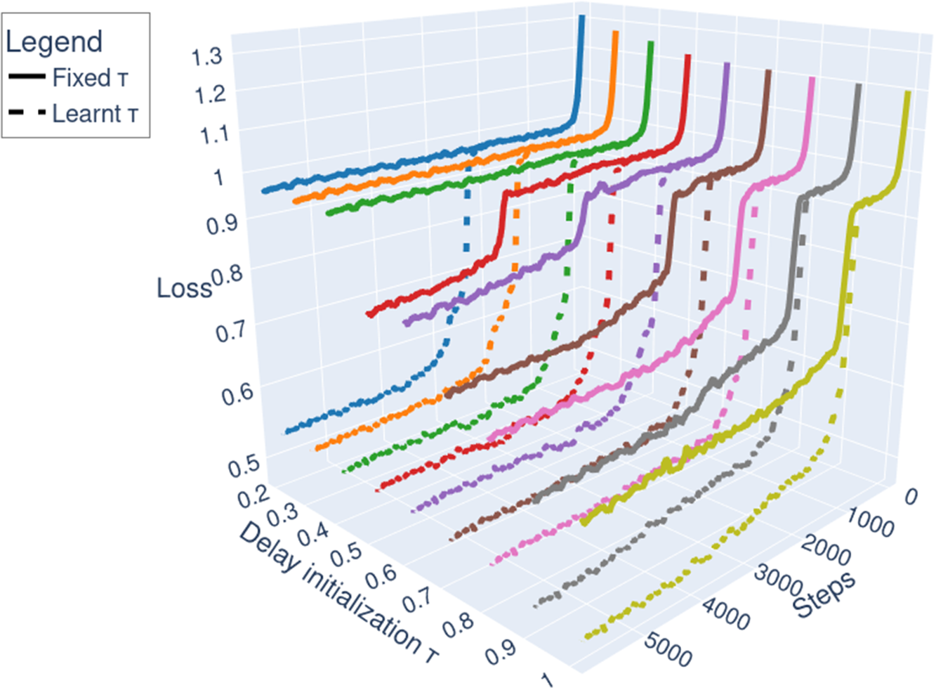
Figure 11. Long description
The 3D line graph has three axes: x-axis labeled Steps ranging from 0 to 5000, y-axis labeled Loss from 0.5 to 1.3, and z-axis labeled Delay initialization tau from 0.2 to 1.0. Each colored pair of lines corresponds to a specific tau value, with solid lines representing fixed tau and dashed lines representing learnt tau, as indicated in the legend at the top left. For each tau value, the loss generally increases with steps, with a sharp rise near the maximum step value. The separation between solid and dashed lines shows the effect of fixed versus learnt delays, with learnt tau (dashed) often showing lower loss than fixed tau (solid) for the same initialization. The colored lines are stacked along the tau axis, with each pair showing a similar trend but at different loss levels. The legend box in the upper left corner specifies line styles: solid for Fixed tau and dashed for Learnt tau.
4.3. Closure modeling with the ROMs
We now revisit the Kuramoto–Sivashinsky configuration from a closure modeling viewpoint. Conceptually, one assumes an accurate model of the system to be known, but the approximate time-dependent solution to be evaluated with a reduced-order model (ROM) Galerkin approach. Specifically, the solution
$ \mathbf{u}(t) $
 is approximated as
$ \mathbf{u}(t)\approx \sum \limits_{i=1}^{N_{\mathrm{terms}}}{\varphi}_i\left(\mathbf{x}\right)\hskip0.1em {a}_i(t) $
is approximated as
$ \mathbf{u}(t)\approx \sum \limits_{i=1}^{N_{\mathrm{terms}}}{\varphi}_i\left(\mathbf{x}\right)\hskip0.1em {a}_i(t) $
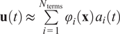 , with
$ {\left\{{\varphi}_i\left(\mathbf{x}\right)\equiv {\boldsymbol{\varphi}}_i\right\}}_{i=1}^{N_{\mathrm{terms}}}=: \Phi $
, with
$ {\left\{{\varphi}_i\left(\mathbf{x}\right)\equiv {\boldsymbol{\varphi}}_i\right\}}_{i=1}^{N_{\mathrm{terms}}}=: \Phi $
 spanning a spatial basis, so that describing the solution boils down to deriving an evolution equation for the coefficients
$ \mathbf{a}(t)=\left({a}_1(t),\dots, {a}_{N_{\mathrm{terms}}}(t)\right) $
spanning a spatial basis, so that describing the solution boils down to deriving an evolution equation for the coefficients
$ \mathbf{a}(t)=\left({a}_1(t),\dots, {a}_{N_{\mathrm{terms}}}(t)\right) $
 . Because the approximation basis
$ \Phi $
. Because the approximation basis
$ \Phi $
 does not span the whole state space whenever
$ {N}_{\mathrm{terms}}<\operatorname{card}\left(\mathbf{u}\right) $
does not span the whole state space whenever
$ {N}_{\mathrm{terms}}<\operatorname{card}\left(\mathbf{u}\right) $
 , the
$ \Phi $
, the
$ \Phi $
 -projected model describing the dynamics of the coefficients
$ {\left\{{a}_i(t)\right\}}_i $
-projected model describing the dynamics of the coefficients
$ {\left\{{a}_i(t)\right\}}_i $
 , resulting from a Galerkin formulation, is not
$ \Phi $
, resulting from a Galerkin formulation, is not
$ \Phi $
 -invariant. To compensate for the loss of information leaking from the subspace spanned by
$ \Phi $
-invariant. To compensate for the loss of information leaking from the subspace spanned by
$ \Phi $
 , one can complement the reduced-order model with an additional, data-based, closure term in the governing equations. Our experiment employs a Galerkin-projected ROM approach, with modes
$ {\left\{{\boldsymbol{\varphi}}_i\right\}}_i $
, one can complement the reduced-order model with an additional, data-based, closure term in the governing equations. Our experiment employs a Galerkin-projected ROM approach, with modes
$ {\left\{{\boldsymbol{\varphi}}_i\right\}}_i $
 derived from a proper orthogonal decomposition (POD), with
$ {N}_{\mathrm{terms}} $
derived from a proper orthogonal decomposition (POD), with
$ {N}_{\mathrm{terms}} $
 = 4, 8, and 10 POD modes (low, medium, and high data regimes), respectively accounting for 58%, 87%, and 94% of the system’s energy (i.e., variance). In practice, the more modes selected in our POD Galerkin ROM, the smaller the correction required by the closure term needs to be.
We now consider different models for representing the closure term and compare their performance in terms of the test MSE loss in Table 4. It is seen that the DDE closure term with learnable delays consistently outperforms the ODE closure term across all data regimes (low, medium, and high). This performance difference becomes especially pronounced in the low data regime of the four-mode POD Galerkin ROM, indicating that the Neural ODE closures are not well-suited for such scenarios. Figure 12, along with their respective representations in the original state space in Figure 13, showcase the prediction from two samples of initial conditions from the test dataset for the four-mode POD Galerkin ROM. As the number of modes increases, the discrepancy between ODE and DDE closures decreases quantitatively, as seen in Table 4. This trend is expected since the ROM then captures most of the system’s information. By studying these specific ROMs, we can identify where ODE closure terms fall short and how incorporating past states with the DDE closure term can address ODE’s deficiencies in low data scenarios. Our approach is compared with the closure model CD-ROM (Menier et al., Reference Menier, Bucci, Yagoubi, Mathelin and Schoenauer2023), which considers a continuous embedding of past information in the form of an exponentially decaying dynamics auxiliary term
$ \mathbf{z}(t) $
 mimicking a memory:

with
$ \Lambda $
 a diagonal matrix whose elements are associated with the relevant time scales of the system under consideration; see (Menier et al., Reference Menier, Bucci, Yagoubi, Mathelin and Schoenauer2023) for details. Interestingly, compared to a memoryless Markovian model such as NODE, it only improves the quality of the prediction in the low-data regime, and considering a higher-dimensional memory variable
$ \mathbf{z}(t) $
a diagonal matrix whose elements are associated with the relevant time scales of the system under consideration; see (Menier et al., Reference Menier, Bucci, Yagoubi, Mathelin and Schoenauer2023) for details. Interestingly, compared to a memoryless Markovian model such as NODE, it only improves the quality of the prediction in the low-data regime, and considering a higher-dimensional memory variable
$ \mathbf{z}(t) $
 does not improve the learning process in high-data regimes.
Summary of model performance metrics, that is, the test MSE loss. CD-ROM, ODE, and DDE closure models are compared across the 4, 8, and 10 POD mode settings

Table 4. Long description
The table has four columns and four rows. The top row lists column headers from left to right as Model, 4 modes, 8 modes, and 10 modes. The first column lists models from top to bottom as C D dash R O M, O D E dash R O M, and D D E dash R O M. For C D dash R O M, the test M S E loss values are 7.94 plus or minus 0.53 for 4 modes, 0.43 plus or minus 0.24 for 8 modes, and 0.099 plus or minus 0.019 for 10 modes. For O D E dash R O M, the values are 13.61 plus or minus 0.34 for 4 modes, 0.44 plus or minus 0.044 for 8 modes, and 0.084 plus or minus 0.0028 for 10 modes. For D D E dash R O M, the values are 3.39 plus or minus 0.034 for 4 modes, 0.18 plus or minus 0.07 for 8 modes, and 0.067 plus or minus 0.0078 for 10 modes. The lowest test M S E loss for each mode count is bolded and occurs for D D E dash R O M at 8 and 10 modes, and for C D dash R O M at 8 modes.
Examples of predictions of POD Galerkin ROM (4 modes).

Figure 12. Long description
Top-left panel a sub 0 plots t on the x-axis and shows four lines: blue dashed for Truth, orange for D D E R O M, green for C D R O M, red for O D E R O M. All lines rise then fall, with Truth and D D E R O M peaking near t equals 20. Top-right panel a sub 1 shows all lines decreasing then oscillating, with Truth and D D E R O M closely aligned. Bottom-left panel a sub 2 shows all lines rising, with Truth and D D E R O M peaking near t equals 20, C D R O M and O D E R O M diverging. Bottom-right panel a sub 3 shows oscillatory behavior, with Truth and D D E R O M closely following each other, C D R O M and O D E R O M diverging after t equals 20. Legend at bottom-right: Truth (blue dashed), D D E R O M (orange), C D R O M (green), O D E R O M (red). Vertical red line at t equals 30 in all panels.
Examples of predictions of POD Galerkin ROM (4 modes) with different models from KS testset reconstructed in terms of the full solution field
$ u\left(\mathbf{x},t\right) $
 (first three columns). The two rightmost columns show the absolute value of the reconstruction error associated with each model.
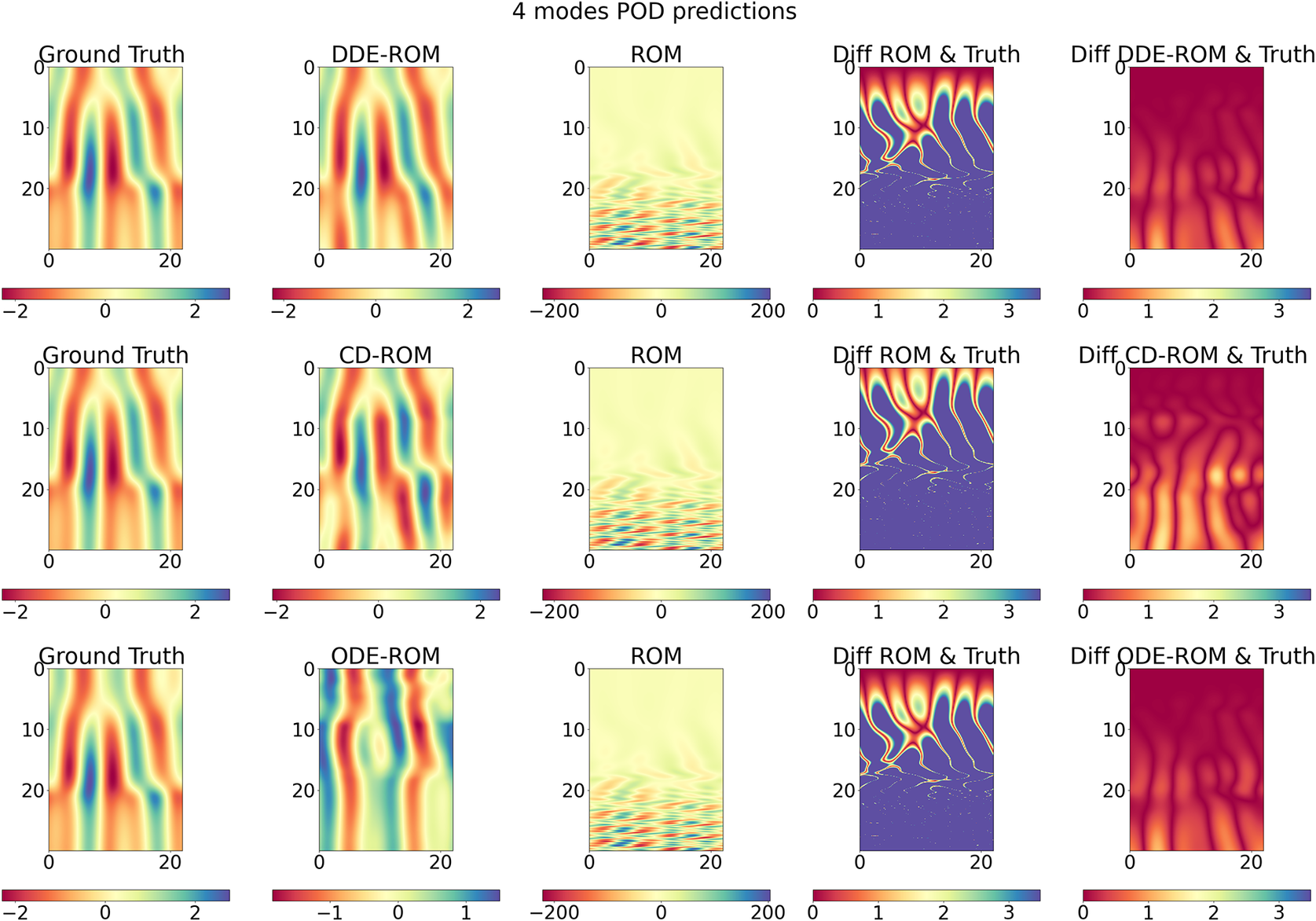
Figure 13. Long description
The grid contains three rows and five columns. Each row starts with a panel labeled Ground Truth showing the reference solution field with a color scale from minus two to two. The next panel in each row displays a model prediction: D D E dash R O M in the first row, C D dash R O M in the second, O D E dash R O M in the third, each with a similar color scale. The third panel in each row shows R O M predictions with a color scale from minus two hundred to two hundred. The fourth panel in each row is labeled Diff R O M and Truth, showing the absolute error between R O M and ground truth, with a color scale from zero to three. The fifth panel in each row shows the absolute error for the specific model versus ground truth: Diff D D E dash R O M and Truth in the first row, Diff C D dash R O M and Truth in the second, Diff O D E dash R O M and Truth in the third, all using a color scale from zero to three. The spatial order is left to right within each row, top row first, followed by the second and third rows. All panels use vertical axes labeled zero to twenty or zero to thirty, and horizontal axes labeled zero to twenty. Color bars are present below each panel, matching the respective value ranges.
Several numbers of learnable delays were considered for the NDDE approach, ranging from 1 to 3. For this system, the results were essentially unaffected by the number of delays, showing that a single delay is enough to recover most of the necessary information for a good prediction.
5. Conclusion
We introduced neural delay differential equations (NDDEs) as a principled and data-efficient framework for modeling partially observed dynamical systems. This approach is motivated on one hand by the Mori–Zwanzig framework first developed in the statistical physics community for accounting for the effect of unobservable quantities on observed ones; and on the other hand by the Takens’ theorem. Relying on these frameworks, we leverage the link between unresolved dynamics and explicit time-delay representations via NDDEs, which allow for a continuous-time, physically interpretable representation of non-Markovian dynamics. In particular, we show that the memory term can be approximated with a finite number of learnable delays without loss of generality under smooth dynamics, providing a compact yet expressive formulation for modeling systems with memory.
Methodologically, we proposed an adjoint-based training procedure for NDDEs with learnable delays, enabling efficient end-to-end optimization over both model parameters and delay variables. The accompanying open-source implementation, torchdde, provides an accessible and reproducible platform for future research and applications.
Numerical and experimental validations are discussed to assess the efficacy of NDDEs across different settings, including synthetic, chaotic, and real-world noisy data, such as the Kuramoto–Sivashinsky equation, and experimental data from cavity-flow configurations. The performed experiments revealed two key insights: first, the pivotal role of a form of memory in accurately capturing dynamics; second, it was demonstrated that LSTMs’ and Latent ODEs’ hidden latent states or ANODEs’ latent variables sometimes fall short in achieving optimal performance, emphasizing the efficacy of delayed terms as an efficient dynamics memory mechanism. In fact, across all scenarios, NDDEs consistently outperformed or matched state-of-the-art continuous-depth and recurrent models while maintaining a smaller parameter footprint and improved interpretability. Finally, we revisited the Kuramoto–Sivashinsky configuration using NDDEs as a closure model of a reduced-order model based on proper orthogonal decomposition modes. With respect to current state-of-the-art closure models, the present approach again exhibits superior performance.
In conclusion, neural delay differential equations provide a theoretically grounded and computationally efficient alternative to traditional recurrent and latent-state neural models for complex non-Markovian dynamical systems. Future research will aim at further generalizing the framework; while overestimating the number of delays does not affect the final performance, rigorously determining the optimal number of delays to consider in NDDE is a challenge. A potentially useful step toward a more principled and meaningful estimation might be achieved by promoting the delayed mutual information between past data and the prediction of future observations (Fraser and Swinney, Reference Fraser and Swinney1986).
Data availability statement
The codes associated with the examples discussed in the article can be found at the following Zenodo-GitHub repository: https://doi.org/10.5281/zenodo.20113438 (Monsel et al., Reference Monsel, Semeraro, Charpiat and Mathelin2026). The torchdde library for learning the delays jointly and the DDE’s dynamics in these models is made open-source at https://doi.org/10.5281/zenodo.20113429 (Monsel et al., Reference Monsel, Menier, Semeraro, Charpiat and Mathelin2026).
Acknowledgments
The authors would like to thank Dr. Emmanuel Menier for helpful discussions.
Author contribution
Conceptualization: T.M., O.S., G.C., and L.M. Methodology: T.M., O.S., G.C., and L.M. Data curation: T.M. Data visualization: T.M. Writing original draft: T.M., O.S., and L.M. All authors approved the final submitted draft.
Funding statement
This work has been funded by the French National Agency for Research under project # ANR-20-CE23-0025-01.
Competing interests
The authors declare none.
Ethical standard
The research meets all ethical guidelines, including adherence to the legal requirements of the study country.
A. Neural IDE and Neural DDE Benchmark
First, let us compare both Neural IDE and Neural DDE analytically, where any function
$ {\mathbf{f}}_{\boldsymbol{\theta}} $
 here denotes a parameterized network:


The second term on the right-hand side of Equation (A.1) is much more computationally involved than the second term on the right-hand side (RHS) of Equation (A.2). Indeed, Equation (A.2) only needs two function evaluations to evaluate its right-hand side, while, on the other hand, the number of function evaluations required to integrate Equation (A.1) increases as
$ t $
 grows to get a correct estimate of the integral term. For a more theoretical examination of computational complexity, one can refer to Appendix A.6 of Monsel et al. (Reference Monsel, Semeraro, Mathelin, Charpiat, Coelho, Zimmering, Costa, Ferrás and Niggemann2024).
A.1. Computation time
Figure A1 compares the computation time of a forward pass between a Neural IDE and Neural DDE, as considered above, of similar size (roughly
$ 500 $
 parameters), with the following setup:
-
• Runge–Kutta 4 (RK4) solver with a timestep of $ dt=0.1 $
 ,
, -
• Batch size of 128,
-
• Neural DDE uses 5 delays,
-
• Different numbers of observations are considered: $ \left\{\mathrm{5,10,50,100}\right\} $
, -
• The upper integration bound is varied from $ t=0.2 $
to
$ t=2.0 $
.


This benchmark clearly shows how expensive Neural IDE is compared to NDDE. NDDEs integration is at least an order of magnitude faster. Note that in Figure A1, the notation “#i” refers to the number of observables
$ {y}_i\left(\mathbf{u},t\right) $
 .
.
Computation time of the forward pass (averaged over 5 runs) as a function of the size of the horizon for different numbers of observations (5, 10, 50, 100).

Figure A1. Long description
The x-axis is labeled Time t, ranging from 0.25 to 2.00. The y-axis is labeled Execution time, shown on a logarithmic scale from 10 super minus 3 to 10 super 0. Eight lines are plotted: solid lines for IDE and dashed lines for DDE, each with four observation counts, indicated by color and legend at the lower right. Blue and orange lines represent 5 observations, green and red for 10, purple and brown for 50, and magenta and gray for 100. For each observation count, the IDE line is consistently above the corresponding DDE line, indicating higher execution time. All lines show a monotonic increase in execution time as t increases, with the gap between IDE and DDE remaining roughly constant for each observation count. The legend lists IDE number 5, DDE number 5, IDE number 10, DDE number 10, IDE number 50, DDE number 50, IDE number 100, and DDE number 100.
A.2. torchdde’s memory and time benchmark
In this subsection, we provide time and memory benchmarks on some of torchdde’s solvers. In order to compare both training methods of optimize-then-discretize (i.e., the adjoint method) and discretize-then-optimize (i.e., regular backpropagation), we present the Brusselator’s experiment time duration and memory usage for various solvers during training (with a batch size of 1024) in Tables A1 and A2, respectively. The adjoint method is slower (by a small factor) and requires less memory than the regular backpropagation. These results are consistent with NODE’s examination of the adjoint method and conventional backpropagation tradeoffs (Chen et al., Reference Chen, Rubanova, Bettencourt, Duvenaud, Bengio, Wallach, Larochelle, Grauman, Cesa-Bianchi and Garnett2018).
Clock time (s) per batch

Table A1. Long description
The table has three rows for RK4, RK2, and Euler algorithms and two columns for Adjoint and Backpropagation methods. For RK4, Adjoint is 4.8 plus or minus 0.23 seconds, Backpropagation is 1.89 plus or minus 0.09 seconds. For RK2, Adjoint is 2.4 plus or minus 0.005 seconds, Backpropagation is 0.90 plus or minus 0.005 seconds. For Euler, Adjoint is 1.5 plus or minus 0.01 seconds, Backpropagation is 0.47 plus or minus 0.003 seconds. All values are in seconds per batch.
GPU consumption (Gb
$ \pm $
 Mb) per batch

Table A2. Long description
From the top row, RK4 lists Adjoint GPU consumption as 2.2 plus or minus 18 gigabytes and Backpropagation as 2.87 plus or minus 4 gigabytes. The next row, RK2, shows Adjoint at 2.15 plus or minus 20 gigabytes and Backpropagation at 2.48 plus or minus 3 gigabytes. The bottom row, Euler, records Adjoint at 2.09 plus or minus 15 gigabytes and Backpropagation at 2.264 plus or minus 9 gigabytes. Across all methods, Adjoint values display greater variance than Backpropagation. Columns are labeled Adjoint and Backpropagation, and rows are labeled RK4, RK2, and Euler.
Figures A2 and A3 compares time and memory consumption for a forward of a Neural DDE with a varying number of delays, respectively, each having ~28,000 parameters. We use the following setup:
-
• Use an RK4 solver with a timestep of $ dt=0.1 $
, -
• Use a batch size of $ 128 $
, -
• Neural DDE uses {1,3,5,10,20} delays,
-
• The number of observations is $ p=100 $
, -
• The upper integration bound is varied from $ t=0.2 $
to
$ t=5.0 $
, -
• The notation “#i” in the figure refers to the number of delays used in the Neural DDE.


Time duration of forward pass averaged over 5 runs.

Figure A2. Long description
The x axis is labeled Time t, ranging from 0 to 5. The y axis is labeled Execution time, using a logarithmic scale from 10 to the negative 2 up to just above 10 to the negative 1. Five dashed lines represent D D E number 1 in blue, D D E number 3 in orange, D D E number 5 in green, D D E number 10 in red, and D D E number 20 in purple. All lines start near the bottom left and rise steeply at first, then more gradually, forming upward curves. D D E number 20 is always the highest, followed by D D E number 10, D D E number 5, D D E number 3, and D D E number 1, which is always the lowest. The legend in the lower right matches line color and style to each D D E number.
Memory consumption of the forward pass averaged over 5 runs.
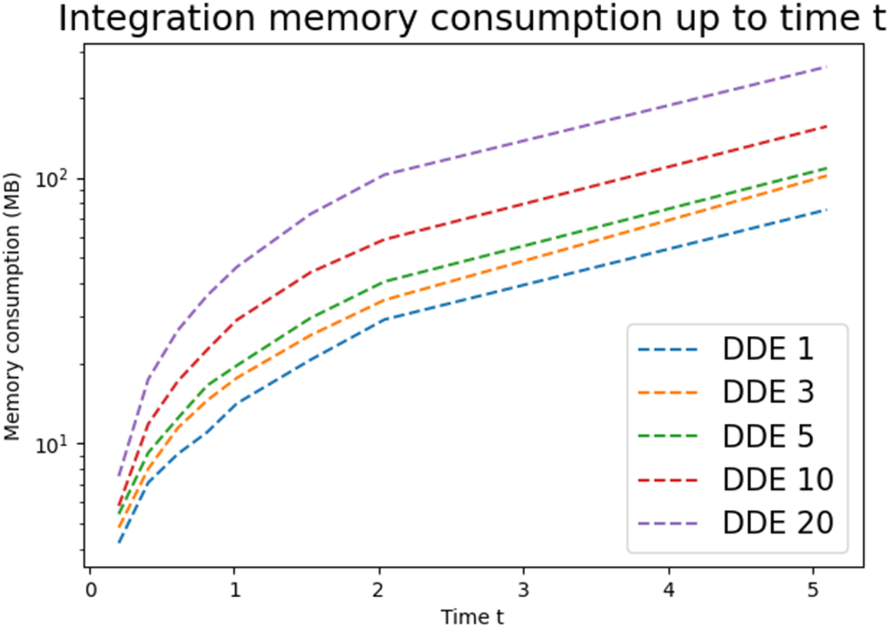
Figure A3. Long description
The x axis is labeled Time t, ranging from 0 to 5. The y axis is labeled Memory consumption in megabytes, using a logarithmic scale from 10 to 100. Five dashed lines represent D D E 1 (blue), D D E 3 (orange), D D E 5 (green), D D E 10 (red), and D D E 20 (purple). All lines show a rapid initial increase in memory consumption, then a slower rise. Higher D D E values consistently result in greater memory consumption at each time point. The legend is located in the lower right quadrant.
B. Derivation of Proposition 3.1
We want to solve the constrained optimization problem introduced in Section 3.1. The delays are part of the learning and are hence a subset of the parameter vector
$ \boldsymbol{\theta} $
 to be optimized. The derivation is first presented for a single delay before being extended to the multiple delay situation below. For convenience, we denote
$ {\mathbf{y}}_{\left(\tau \right)}(t) $
to be optimized. The derivation is first presented for a single delay before being extended to the multiple delay situation below. For convenience, we denote
$ {\mathbf{y}}_{\left(\tau \right)}(t) $
 the third set of variables that
$ {\mathbf{h}}_{\boldsymbol{\theta}}\left(t,\mathbf{y}(t),\mathbf{y}\left(t-\tau \right)\right) $
the third set of variables that
$ {\mathbf{h}}_{\boldsymbol{\theta}}\left(t,\mathbf{y}(t),\mathbf{y}\left(t-\tau \right)\right) $
 depend on, and with a dot, the time derivative
$ \dot{\mathbf{z}}(t) $
depend on, and with a dot, the time derivative
$ \dot{\mathbf{z}}(t) $
 of any quantity
$ \mathbf{z}(t) $
of any quantity
$ \mathbf{z}(t) $
 . To recall, we consider the following minimization problem:

We consider the following Lagrangian
$ \mathcal{L} $
 :
:

We use
$ \mathbf{y}\left(t-\tau \right)={\mathbf{y}}_{\left(\tau \right)}(t) $
 wherever convenient. At optimality, the state equation is satisfied (
$ \mathbf{y} $
wherever convenient. At optimality, the state equation is satisfied (
$ \mathbf{y} $
 is a solution to the associated DDE), implying that
$ \frac{\partial \mathcal{L}}{\partial \boldsymbol{\theta}}=\frac{\partial L}{\partial \boldsymbol{\theta}} $
is a solution to the associated DDE), implying that
$ \frac{\partial \mathcal{L}}{\partial \boldsymbol{\theta}}=\frac{\partial L}{\partial \boldsymbol{\theta}} $
 .
.
Integration by parts of the expression of the Lagrangian (Eq. (B.2)) yields:

Stationarity of the Lagrangian at optimality yields
$ \frac{\partial \mathcal{L}}{\partial \mathbf{y}}=\mathbf{0} $
 and expressed as:

With the change of variable
$ t\to t-\tau $
 , the fourth term of the integrand rewrites as:

where we have set
$ \boldsymbol{\lambda} (t)=\mathbf{0} $
 whenever
$ t\ge T $
whenever
$ t\ge T $
 and recognized that
$ \mathbf{y}\left(t\le {t}_0\right)\equiv \boldsymbol{\psi} (t) $
and recognized that
$ \mathbf{y}\left(t\le {t}_0\right)\equiv \boldsymbol{\psi} (t) $
 with
$ \frac{\partial \boldsymbol{\psi} (t)}{\partial \mathbf{y}}=\mathbf{0} $
with
$ \frac{\partial \boldsymbol{\psi} (t)}{\partial \mathbf{y}}=\mathbf{0} $
 .
.
The boundary terms
$ \frac{\partial {\left[\boldsymbol{\lambda} (t)\mathbf{y}(t)\right]}_{t_0}^T}{\partial \mathbf{y}} $
 in Eq. (B.4) then vanish, and the equation is satisfied whenever the integrand is identically zero. Hence, the following adjoint equation, to be integrated backwards in time:

Now, taking the derivative of the Lagrangian with respect to θ expresses:

Since
$ \frac{\partial \mathbf{y}}{\partial \boldsymbol{\theta}}\equiv \mathbf{0} $
 and owing to the adjoint dynamics in Equation (B.6), it finally comes

B.1. Case for multiple constant delays
In the case of multiple delays
$ {\tau}_i $
 ,
$ i\in 1,\dots, n $
,
$ i\in 1,\dots, n $
 , the equations in Theorem 3.1 are extended as follows. For each
$ i $
, the equations in Theorem 3.1 are extended as follows. For each
$ i $
 , we define
$ {\mathbf{y}}_{\left({\tau}_i\right)}(t)\equiv \mathbf{y}\left(t-{\tau}_i\right) $
, we define
$ {\mathbf{y}}_{\left({\tau}_i\right)}(t)\equiv \mathbf{y}\left(t-{\tau}_i\right) $
 .
.
The second term
$ \boldsymbol{\lambda} (t)\frac{\partial {f}_{\boldsymbol{\theta}}\left(t,\mathbf{y}(t),{\mathbf{y}}_{\left(\tau \right)}(t)\right)}{\partial \mathbf{y}} $
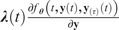 in the adjoint dynamics (Eq. (B.6)) is replaced by:

and the last term
$ \boldsymbol{\lambda} \left(t+\tau \right)\frac{\partial {f}_{\boldsymbol{\theta}}\left(t+\tau, \mathbf{y}\left(t+\tau \right),{\mathbf{y}}_{\left(\tau \right)}\left(t+\tau \right)\right)}{\partial {\mathbf{y}}_{\left(\tau \right)}} $
 by the following:

The first term
$ \frac{\partial {f}_{\boldsymbol{\theta}}\left(t,\mathbf{y}(t),{\mathbf{y}}_{\left(\tau \right)}(t)\right)}{\partial \boldsymbol{\theta}} $
 in the gradient’s Equation (B.8) becomes

and
$ \frac{\partial {f}_{\boldsymbol{\theta}}\left(t,\mathbf{y}(t),{\mathbf{y}}_{\left(\tau \right)}(t)\right)}{\partial {\mathbf{y}}_{\left(\tau \right)}}\frac{\partial \mathbf{y}\left(t-\tau \right)}{\partial \boldsymbol{\theta}} $
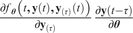 is now:

C. Derivation of Proposition 2.1
Let us start by stating Takens’ theorem as expressed by Takens (Reference Takens, Rand and Young1981)), Noakes (Reference Noakes1991)):
Theorem C.1 (Takens’ embedding theorem). Let
$ \mathcal{M} $
 be a compact space. There is an open dense subset
$ \mathcal{D} $
be a compact space. There is an open dense subset
$ \mathcal{D} $
 of
$ \mathrm{Diff}\left(\mathcal{M}\right)\times {C}^2\left(\mathcal{M},\unicode{x211D}\right) $
of
$ \mathrm{Diff}\left(\mathcal{M}\right)\times {C}^2\left(\mathcal{M},\unicode{x211D}\right) $
 , with
$ \mathrm{Diff}\left(\mathcal{M}\right) $
, with
$ \mathrm{Diff}\left(\mathcal{M}\right) $
 the diffeomorphism group of
$ \mathcal{M} $
the diffeomorphism group of
$ \mathcal{M} $
 , with the property that the Takens map

given by
$ \mathfrak{y}\left(\mathbf{u}\right)=\left(\mathbf{y}\left(\mathbf{u}\right),\mathbf{y}\left(\phi \left(\mathbf{u}\right)\right),\mathbf{y}\left(\phi \circ \phi \left(\mathbf{u}\right)\right),\dots, \mathbf{y}\left({\phi}^{2m}\left(\mathbf{u}\right)\right)\right) $
 is an embedding of
$ {C}^2 $
is an embedding of
$ {C}^2 $
 manifolds, where
$ \left(\phi, \mathbf{y}\right)\in \mathcal{D} $
manifolds, where
$ \left(\phi, \mathbf{y}\right)\in \mathcal{D} $
 .
.
Here,
$ \phi $
 stands for the operator that advances the dynamical system by a time step
$ \tau $
stands for the operator that advances the dynamical system by a time step
$ \tau $
 , i.e., that sends
$ \mathbf{u}(t) $
, i.e., that sends
$ \mathbf{u}(t) $
 to
$ \mathbf{u}\left(t+\tau \right) $
to
$ \mathbf{u}\left(t+\tau \right) $
 , and
$ \mathbf{y} $
, and
$ \mathbf{y} $
 is the observable operator that sends a full state
$ \mathbf{u}(t) $
is the observable operator that sends a full state
$ \mathbf{u}(t) $
 to actual observables
$ \mathbf{y}\left(\mathbf{u}(t)\right)=: \mathbf{y}(t) $
to actual observables
$ \mathbf{y}\left(\mathbf{u}(t)\right)=: \mathbf{y}(t) $
 . Variants of this Theorem, for example, Sauer et al. (Sauer et al., Reference Sauer, Yorke and Casdagli1991), include the consideration of any set of different delays
$ {\tau}_i $
. Variants of this Theorem, for example, Sauer et al. (Sauer et al., Reference Sauer, Yorke and Casdagli1991), include the consideration of any set of different delays
$ {\tau}_i $
 instead of uniformly spaced ones. The representation
$ \mathfrak{y}\left(\mathbf{u}(t)\right)=\Big(\mathbf{y}\left(\mathbf{u}(t)\right),\mathbf{y}\left(\mathbf{u}\left(t-\tau \right)\right),\mathbf{y}\left(\mathbf{u}\left(t-2\tau \right)\right),\dots \mathbf{y}\left(\mathbf{u}\left(t-2 m\tau \right)\right) $
instead of uniformly spaced ones. The representation
$ \mathfrak{y}\left(\mathbf{u}(t)\right)=\Big(\mathbf{y}\left(\mathbf{u}(t)\right),\mathbf{y}\left(\mathbf{u}\left(t-\tau \right)\right),\mathbf{y}\left(\mathbf{u}\left(t-2\tau \right)\right),\dots \mathbf{y}\left(\mathbf{u}\left(t-2 m\tau \right)\right) $
 then becomes
$ \mathfrak{y}\left(\mathbf{u}(t)\right)=\Big(\mathbf{y}\left(\mathbf{u}(t)\right),\mathbf{y}\left(\mathbf{u}\left(t-{\tau}_1\right)\right),\mathbf{y}\left(\mathbf{u}\left(t-{\tau}_2\right)\right),\dots \mathbf{y}\left(\mathbf{u}\left(t-{\tau}_{2m}\right)\right) $
then becomes
$ \mathfrak{y}\left(\mathbf{u}(t)\right)=\Big(\mathbf{y}\left(\mathbf{u}(t)\right),\mathbf{y}\left(\mathbf{u}\left(t-{\tau}_1\right)\right),\mathbf{y}\left(\mathbf{u}\left(t-{\tau}_2\right)\right),\dots \mathbf{y}\left(\mathbf{u}\left(t-{\tau}_{2m}\right)\right) $
 . In the proof of Takens’ theorem,
$ m $
. In the proof of Takens’ theorem,
$ m $
 is the intrinsic dimension of the dynamical system, that is, the dimension of the manifold
$ \mathcal{M} $
is the intrinsic dimension of the dynamical system, that is, the dimension of the manifold
$ \mathcal{M} $
 .
.
Now, given the full state
$ \mathbf{u} $
 that follows the dynamics:

we use the chain rule on the observable
$ \mathbf{y} $
 :
:

By applying the inverse of the delay coordinate map
$ {\mathfrak{y}}^{-1} $
 from Theorem C.1, which is invertible from its image as it is an embedding, we show that the dynamics of
$ \mathbf{y} $
from Theorem C.1, which is invertible from its image as it is an embedding, we show that the dynamics of
$ \mathbf{y} $
 possess a DDE structure:

The proof is completed by choosing
$ \mathbf{h}=\left({\mathbf{y}}^{\prime}\times \mathbf{f}\right)\circ {\mathfrak{y}}^{-1}-M $
 where
$ M $
where
$ M $
 is obtained by the Mori–Zwanzig formalism (Eq. (2.6)).
Note that to be able to apply Takens’ theorem, we needed the step-forward operator
$ \phi $
 to be a diffeomorphism, that is, the flow of the dynamical system to be smooth and smoothly invertible. Also, we used the differentiability of the observables
$ \mathbf{y} $
to be a diffeomorphism, that is, the flow of the dynamical system to be smooth and smoothly invertible. Also, we used the differentiability of the observables
$ \mathbf{y} $
 to express
$ {\mathbf{y}}^{\prime } $
to express
$ {\mathbf{y}}^{\prime } $
 .
.
D. Training hyperparameters
Our training approach incorporates a progressive strategy considered to be a curriculum learning strategy (Soviany et al., Reference Soviany, Ionescu, Rota and Sebe2022). We begin by feeding the models shorter trajectory segments and gradually increase their length when the so-called patience hyperparameter is exceeded. This process continues until we reach the desired trajectory length. Each time the trajectory length is increased, we reset the patience hyperparameter to 0. This patience is then incremented by 1 if the validation loss fails to decrease, and reset to 0 if the validation loss improves. This method aligns with the principles of curriculum learning, a technique that involves training machine learning models in a structured order, typically progressing from simpler to more complex examples. In our case, this translates into moving from shorter to longer trajectories. This approach aims to improve the learning process and the resulting model performance. Table A3 displays the patience parameter and the length of the trajectory considered initially. Table A4 refers to the number of training parameters of each model. The loss function used across all experiments is the MSE loss, and we employ the Adam optimizer with a weight decay of
$ {10}^{-7} $
 . Table A5 provides the initial and final learning rates (
$ {\eta}_i $
. Table A5 provides the initial and final learning rates (
$ {\eta}_i $
 ,
$ {\eta}_f $
,
$ {\eta}_f $
 ) for each experiment, which are associated with the scheduler. The scheduler is a StepLR scheduler with a gamma factor (
$ \gamma =\exp \left(\frac{\log \left({\eta}_f/{\eta}_i\right)}{N}\right) $
) for each experiment, which are associated with the scheduler. The scheduler is a StepLR scheduler with a gamma factor (
$ \gamma =\exp \left(\frac{\log \left({\eta}_f/{\eta}_i\right)}{N}\right) $
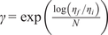 , with
$ N $
, with
$ N $
 the trajectory’s length). The scheduler adjusts the learning rate as the trajectory length increases, allowing training to start with the initial learning rate
$ {\eta}_i $
the trajectory’s length). The scheduler adjusts the learning rate as the trajectory length increases, allowing training to start with the initial learning rate
$ {\eta}_i $
 and gradually decrease to the final learning rate
$ {\eta}_f $
and gradually decrease to the final learning rate
$ {\eta}_f $
 . All continuous-time models (NODE, ANODE, Latent ODE, and NDDE) used Runge–Kutta for numerical integration. Table A6 shows the width and depth of the multi-layer perceptrons (MLPs) for NODE, ANODE, and NDDE across all experiments. Additionally, we provide the hidden size and number of layers for the LSTM model in Table A7. Finally, Table A8 summarizes the Latent ODE hyperparameters, where the vector field
$ {f}_{\boldsymbol{\theta}} $
. All continuous-time models (NODE, ANODE, Latent ODE, and NDDE) used Runge–Kutta for numerical integration. Table A6 shows the width and depth of the multi-layer perceptrons (MLPs) for NODE, ANODE, and NDDE across all experiments. Additionally, we provide the hidden size and number of layers for the LSTM model in Table A7. Finally, Table A8 summarizes the Latent ODE hyperparameters, where the vector field
$ {f}_{\boldsymbol{\theta}} $
 (defined in the Introduction) is an MLP with the width and depth specified in the second and third columns, respectively, the size of the latent variable
$ {z}_0 $
(defined in the Introduction) is an MLP with the width and depth specified in the second and third columns, respectively, the size of the latent variable
$ {z}_0 $
 in the last column, and the RNN’s hidden size in the fourth column. If some models have fewer parameters compared to others, it is because we found that they provided better results with fewer. ANODE’s augmented state dimension matches that of the number of delays used by NDDE displayed in Table 1.
How long are the trajectory chunks given at first, and the patience used for each experiment

Table A3. Long description
The table has three columns for experiments: K S, Cavity, and Brusselator. The first row labeled Length start lists 15 percent for K S, 50 percent for Cavity, and 25 percent for Brusselator. The second row labeled Patience lists 40 for K S, 50 for Cavity, and 20 for Brusselator. Each value is aligned under its respective experiment.
Number of parameters for each experiment

Table A4. Long description
The table has three rows for experiments: Brusselator, K S, and Cavity. For Brusselator, parameter counts are L S T M 1764, N O D E 3265, A N O D E 3395, Latent O D E 3666, N D D E 3331. For K S, L S T M 18130, N O D E 9029, A N O D E 11609, Latent O D E 8118, N D D E 19343. For Cavity, L S T M 2234, N O D E 2209, A N O D E 2274, Latent O D E 3642, N D D E 2242. Columns are ordered left to right as L S T M, N O D E, A N O D E, Latent O D E, N D D E. Each cell contains the parameter count for the corresponding model and experiment.
Initial and final learning rates for each experiment

Table A5. Long description
The table has three columns. The first column lists experiments: Brusselator, Cavity, K S, and Shallow water. The second column, labeled eta sub i, gives initial learning rates: 0.001 for Brusselator, 0.005 for Cavity, 0.01 for K S, and 0.001 for Shallow water. The third column, labeled eta sub f, gives final learning rates: 0.0001 for Brusselator, 0.00005 for Cavity, 0.0001 for K S, and 0.00001 for Shallow water. Each row aligns experiment name with its corresponding initial and final learning rates.
MLP width and depth for each experiment

Table A6. Long description
From the top row downward, the left column lists experiment names: Brusselator, K S, Cavity, and Shallow Water. The middle column shows width values: 32 for Brusselator, 64 for K S, 32 for Cavity, and 32 for Shallow Water. The right column displays depth values: 4 for Brusselator, 3 for K S, 3 for Cavity, and 3 for Shallow Water. The column headers above are NODE slash ANODE slash N D D E, with sub-headers for Width and Depth.
Hidden size and number of layers for each experiment for the LSTM model

Table A7. Long description
The table has three columns labeled Experiment, Hidden size, and Number of layers. From top to bottom, the first row lists Brusselator with hidden size 5 and number of layers 10. The second row lists K S with hidden size 25 and number of layers 5. The third row lists Shallow water with hidden size 6 and number of layers 10. The fourth row lists Cavity with hidden size 7 and number of layers 7. All values are aligned with their respective experiments.
Configuration parameters for each experiment for Latent ODE

Table A8. Long description
The header row lists Experiment, Width size, Depth, Hidden size, and Latent size from left to right. The first row is Brusselator with width size 16, depth 3, hidden size 16, latent size 16. The second row is K S with width size 32, depth 3, hidden size 16, latent size 16. The third row is Cavity with width size 16, depth 3, hidden size 8, latent size 8. The fourth row is Shallow water with width size 32, depth 3, hidden size 8, latent size 8.
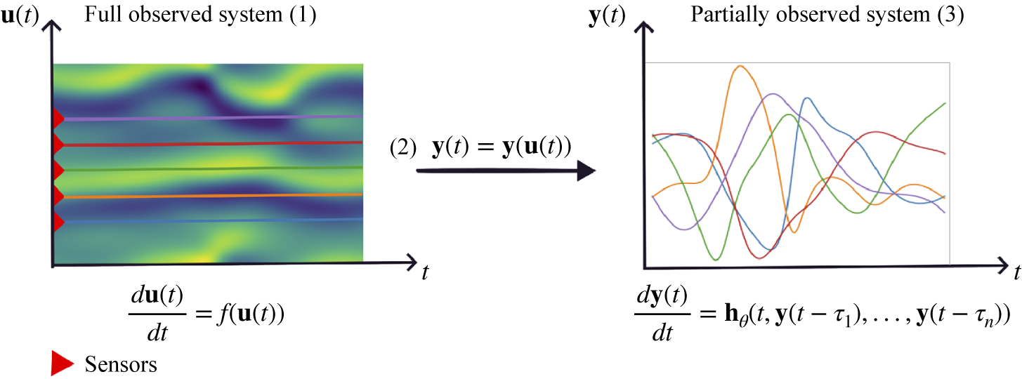

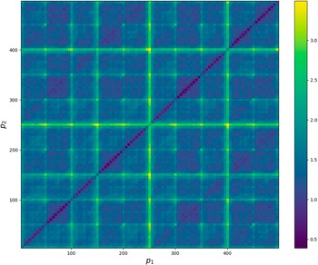



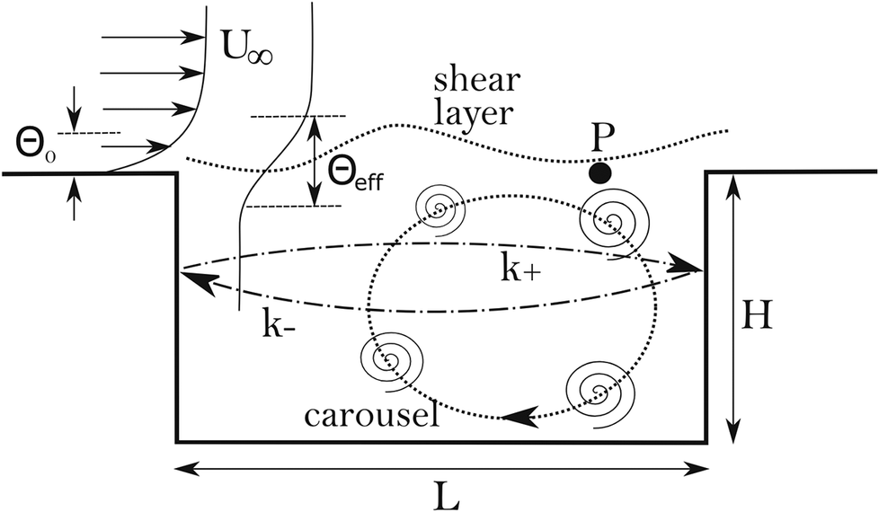



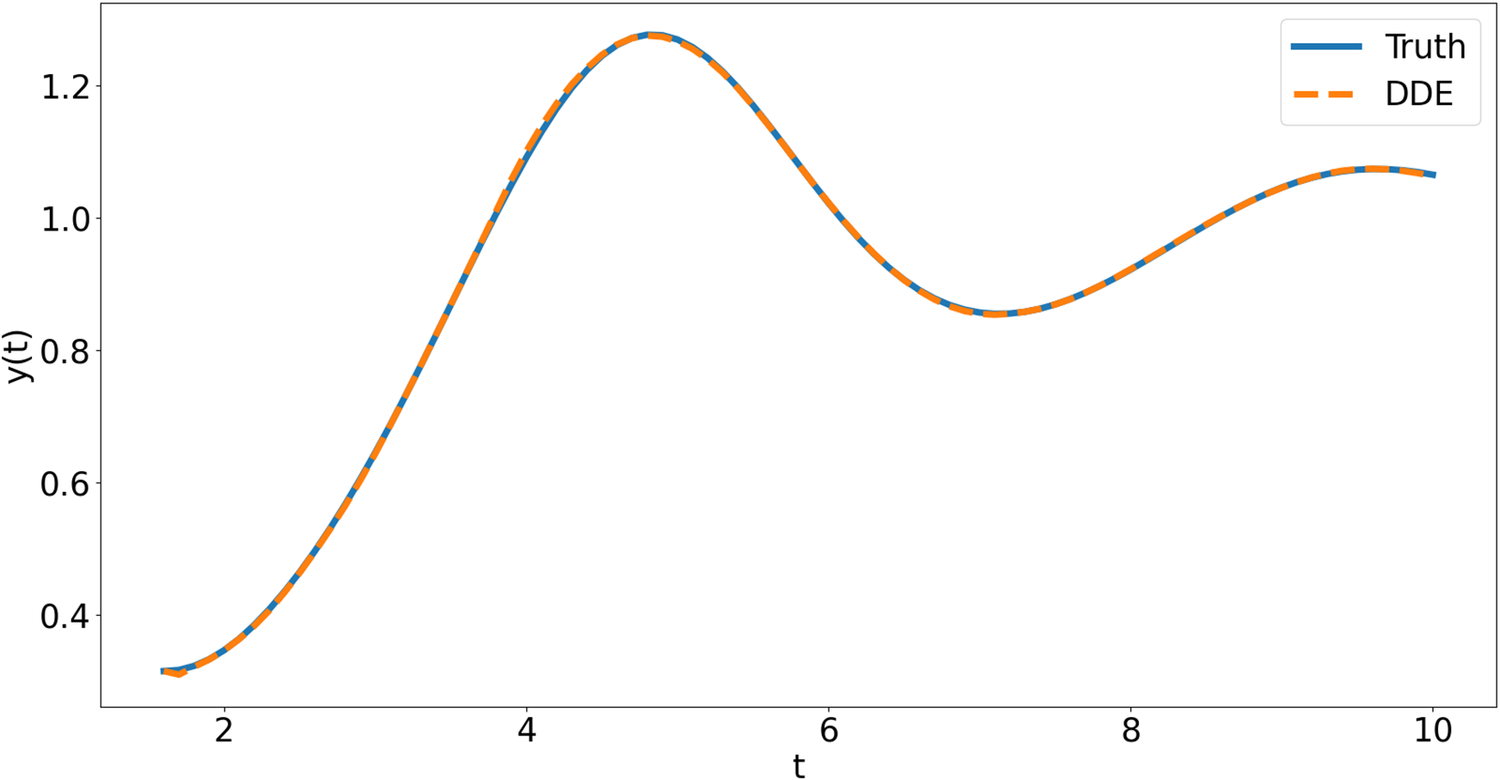
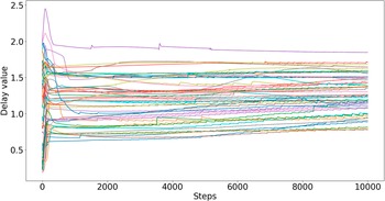
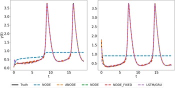

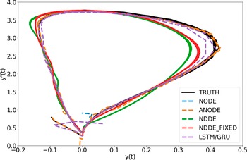

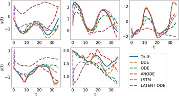
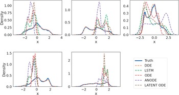



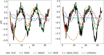



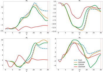
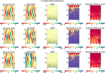

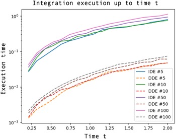



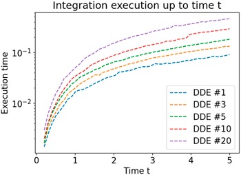
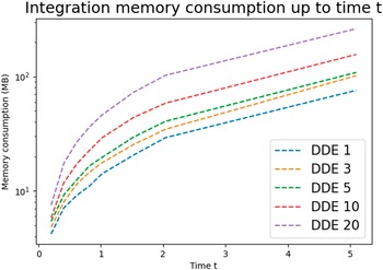



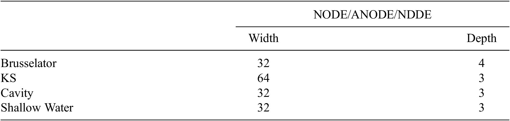



 Open access


Comments
No Comments have been published for this article.