


Introduction
Part–whole relationships are essential to creating designs, composing them, and getting them fitting together. Forms are understood from their independently significant parts. In architecture, a grammar of form helps us get the sense of detail, compose large structures by assembling parts, and fitting them into their setting. Moreover, because our natural awareness of symmetry and proportion affects how we perceive architecture, discriminating and associating building parts and wholes is critical. In every design judgment, we seek technical, aesthetic, or semantic criteria and rule guidedness to enable us to judge part–whole relationships. Sometimes these criteria are a byproduct of previous successful resolutions. Other times we improvise. In both cases, determining part–whole relationships is the task of design. It is about how shapes are perceived by their parts and how parts fit to serve various purposes.
Shapes are perceived unanalyzed, without rigid representation of their parts. This feature of shapes enables countless types of exploration. We parse shapes into parts based on explicit interests and use them to describe things. An elemental design method is converting unanalyzed shapes into structured descriptions of significant parts and back to wholes. This paper offers an account of the part–whole figuration process based on shape grammar formalism. To this end, four compositions with shapes made out of lines are constructed, and an identity rule is used to illustrate a specific way of perceiving their parts. Shape decompositions having structures of topologies and Boolean algebras are used to illustrate the development of parts locally and globally in the course of the four computations.
A shape decomposition presents a shape as a finite, nonempty set of parts that add to the shape. In design, we break shapes into parts, organize their structures, interpret their attributes, and then forget or discard them. Everything is fused back to a unified whole, and we start anew in an iterative process that moves to an unforeseen conclusion based on observation, reflection, and imagination. Earl (Reference Earl1999) concludes that design descriptions are intertwined with the generative history of a design: “Descriptions are woven through the generative history of a design; created, composed, and discarded. The algebra of structure and composition is key to analyzing the freedoms and constraints in generative design systems.” The generative history of a design is a history of continuous transition. Forgetting and revising structure is instrumental in this process, though in systems that compute with symbolic descriptions are complex to attain. Descriptions with lines, planes, or solids serve this process admirably since they do not inherently convey any syntactic information. The viewer introduces structure by interpreting their appearance in diverse ways, and even though shapes are conveniently finite, they can receive infinitely many interpretations. Stiny (Reference Stiny2022) offers an explanation on how this works computationally: “Every shape is the synthesis of a thesis and an antithesis, but the shape/synthesis doesn't care about these opposing descriptions or visual analogies. There are ‘myriad myriads’ like them primed for instant use. All of these save the appearances.” A drawing lacks internal, atomic structure in the depiction of entities. It is a synthesis of elements, and there is no built-in way of ordering these elements to maintain a structure, like a set. Synthesis is what Stiny calls “the effect of reducing” multiple descriptions to a single shape. Technically, it is the same as using “reduction rules” in shape grammars to embed and fuse shape parts.
Drawing on geometrical analogies originating in the Pythagoreans and the German dialectic tradition, the English poet Samuel Taylor Coleridge ascribes “indifference” to synthesizing two opposing descriptions, a thesis and an antithesis. Coleridge's Method “supposes a principle of unity with progression.” It applies to alive things growing in nature and promotes the soul's growth. The Method aims to reach higher degrees of synthesis through transition, not by forgetting polarities but by synthesizing them. In his Essays on the Principles of Method (1818), Coleridge explains more: “Method implies a progressive transition, and it is the meaning of the word in the original language. The Greek Μέθοδος is literally a way, or path of Transit … without continuous transition, there can be no Method … The term, Method, cannot therefore, otherwise than by abuse, be applied to a mere dead arrangement, containing in itself no principle of progression” (Coleridge, Reference Coleridge and Rooke1969, iv, 457). Likewise, a generative design process – though perhaps not every generative design process – is a transition, not a dead arrangement. Shapes are a good fit for continuous progressive transition, while symbols are suitable for arrangement and re-arrangement. The continuous transition of shape parts and wholes in descriptions resembles Coleridge's Method. It is formalized in shape grammars via the embed-fuse cycle (Stiny, Reference Stiny2022), where numerous shapes disappear without preserving any discrete parts, and analysis and synthesis are connected in a single recursive process through parts ≤ and sums (+). Forgetting all prior structure is critical; otherwise, the progressive transition is unattainable, and synthesis is reduced to a mere arrangement.
The Method of Coleridge and the formal approach of the embed-fuse cycle (Stiny, Reference Stiny2022) are used in this paper to elucidate a simple design exercise. An initial square containing four maximal lines is progressively modified in the presented four computations by adding and translating squares along the horizontal axis. At each computational step, shapes fuse into a synthesis without preserving any discrete parts, and a single identity rule is applied to present all squares. Shape decompositions having structures of topologies and Boolean algebras are constructed based on this identity rule. Topologies depict alternative structures of lines for shapes that enable the comparison and relativization of parts, and lattice diagrams present their order. Retrospectively, the topologies are used to recall the design's generative history and establish continuity for all four computation steps. In the course of the four steps, topologies change in unpredictable ways as emergent squares are recognized. When the parts are modified to serve the local recognition of squares, other emergent shapes are highlighted globally, as the topology of the whole is re-adjusted. How we see the local parts modifies how we analyze the global whole, and thus, a local observation yields a global structure. Accordingly, two types of emergence are identified: local and global. The use of local and global emergence and structure is central in this paper. Furthermore, contrary to the standard conviction that innovation depends on the variety of rules and complexity of representations (data), it is confirmed that reducing rule variety and descriptive complexity to a bare minimum – a single identity rule and simple lines – can have broad constructive implications on part–whole figuration, provided that shapes are not restricted by representation.
The presented visual examples elaborate Lionel March's exposition of a single-rule shape grammar translating triangles in Rulebound Unruliness, published in Environment and Planning B: Planning and Design in 1996. This new treatment offers some new formal grounding based on recent developments in shape computation by observing shape decomposition and relativization of structure. March (Reference March1996) contrasts the macro-behavior of atoms in cellular automata and fractals against a single-rule shape grammar capable of generating shape worlds. He revisits the Lucretian model of parallel translation of a stream of atoms. Ιn the Lucretian model, the atoms constantly move in parallel at the same speed and direction, without interacting unless the clinamen's random perturbation is introduced. In the shape grammatical model, equilateral triangles move in one of three directions based on the triangle's threefold symmetry, and interaction occurs under translation without the need for random perturbation. March notices that the macro-behavior of atoms in cellular automata and fractals is conceived in grids and point sets. The shape grammar approach neither requires a grid nor is tied to point sets. Furthermore, cellular automata and fractals operate under globally applied rules, whereas most shape grammars apply locally when a sub-shape is selected for a rule application: “there is emergence among nonatomic shapes, in which rules are applied locally and serially, not globally and in parallel.” In this sense, local spatial relations determine the global possibilities. Moreover, the decision tree of rule applications is not binary.
In this demonstration, a square instead of a triangle is modified by adding and translating squares horizontally. In March's words: “when two triangles [squares] intersect, there is the possibility that additional triangles [squares] will emerge. This characteristic of shapes gives rise to spontaneous creation (or destruction).” The identity rule recognizing squares offers spontaneous creation by structuring the shape and allowing new sub-shapes in the same topology to get noticed. However, each observed structure is temporary. The four consecutive descriptions resolve in a single synthesis of maximal lines without preserving any parts. The retrospective generative history of the computation is a history of reconciling structures, two at the time a thesis and an antithesis, by revising their topologies. A topology for the entire computation is configured backward at the end so that the rule application is continuous in the four steps, and a kit of parts is furnished that works throughout, turning shapes into sets.
Finally, the somewhat inflammatory title Design without Representation references Rodney Brook's paper Intelligence without Representation published in Artificial Intelligence Journal in 1991. Although Brooks comes from artificial intelligence (AI) and robotics, AI and computational design have foundered on representation. Representation refers to the technical problem of encoding knowledge and reasoning into a symbolic language that enables it to be processed by information systems. Deeming that human intelligence is too complex and little understood to be fully decomposed into the correct sub-pieces right from the start, Brooks suggests decomposing an intelligent system into independent, parallel activity producers, which interface directly to the world through perception and action. “When intelligence is approached with strict reliance on interfacing to the real world through perception and action, reliance on representation disappears.” Since there is no central unit system, there is no need for global representation. However, despite the provocative title Brooks proposes multiple low-level representations distributed in multiple activity-producing subsystems instead of an overarching, high-level representation. In the end, he admits that: “a careful reading shows that I mean intelligence without conventional representation, rather than without any representation at all.”
One may argue that design intelligence is similarly complex and poorly understood to be accurately decomposed into permanent sub-domains. Furthermore, design intelligence does not depend on information processing because design is not communication but construction. It is better understood as a process of transition that requires activity and interfacing to the world through perception and action. A designer transitions spontaneously from one drawing to another. Lines and planes provide rough material for these transitions. The viewer imposes structure by looking, and structure lasts until a new stroke or subdivision is introduced. As Stiny (Reference Stiny2022) puts it: “seeing supersedes description.” In this sense, a drawing's primary purpose is constructing a design rather than communicating it. Knowledge representation relies on symbolic encoding to be processed by a computer agent and used in automated reasoning. Without representation, there is no information to process. Even though automated reasoning serves the quantitative design aspects, the creative, qualitative aspects demand a different approach. A shape is first distinguished by appearance and then structured by dividing and fusing parts, which is the concern of this paper. A shape structure is attributed at the end, not in the beginning. Therefore, a shape fails to satisfy knowledge representation criteria. Its principal usefulness is appearance. Turning appearance into information to enable automated processing removes perception and turns a visual material into a symbolic representation. While Brooks suggests that an overarching, high-level symbolic representation is unnecessary in order for a system to realize intelligent behavior, Stiny emphasizes the transformational value of seeing and installs visual perception at the core of design intelligence via the embed-fuse cycle, “which unifies and re-divides (creates), to supersede lifeless representation.” The paper shows that removing representation is necessary for saving appearance by demonstrating a simple example of shape computation.
Shapes, algebras, rules, and decompositions
The shape grammar theory was introduced in the 70s (Stiny and Gipps, Reference Stiny, Gipps and Freiman1972), and it was refined through thought-provoking research for five decades. A comprehensive recapitulation of shape formalism exists in Stiny (Reference Stiny2006). Shape formalism demonstrates how a corpus of spatial configurations can be computed with rules in a recursive process. A shape grammar generates a set of shapes by capturing the interaction of basic elements of 0, 1, 2, or 3 dimensions. Shape grammars include an algebraic and a syntactic-interpretive part. The algebraic part offers a framework for calculating with shapes, such as addition, subtraction, and product. The syntactic-interpretive part consists of productive rule statements assigning structure and meaning to computations.
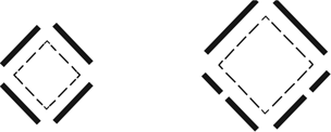
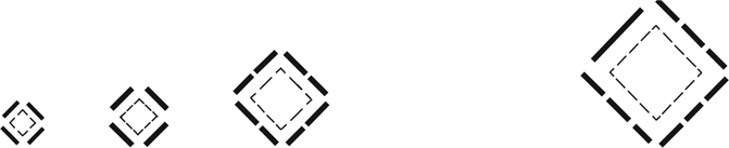
A shape is a finite arrangement of elements of 0, 1, 2, or 3 dimensions organized in a finite space of 1, 2, or 3 dimensions. Shape elements are maximal so that no two elements of the same dimension combine to make a third element that contains the two (Fig. 1). For example, a standard description of a square is four lines that are divisible in infinitely many ways. However each time we treat finitely many parts.
A standard description of a square (left) is four maximal lines (center). They are divisible in infinitely many ways, but each time we treat finitely many parts (right).

The algebraic framework of shape grammars includes algebras of shapes. An algebra is a set of elements that are closed under a set of operations. A shape algebra uses shapes to calculate. Algebras can be distributive or associative, while axioms can distinguish other algebraic structures like rings, lattices, and Boolean algebras. A sub-algebra is a non-empty subset of an algebra U that is also an algebra, given that it is closed under the same operations of union, difference, and the intersection of the algebra U.
An algebra Uij includes i-dimensional shapes in a j-dimensional space, with i ≤ j and i = 0, 1, 2, and 3 for points, lines, planes, and solids. Euclidean transformations t, such as isometries or similarities, are included in the algebras. Krstic (Reference Krstic1999, Reference Krstic2014) proposes two alternative algebraic structures for incorporating the transformations in the algebras Uij. The first incorporates transformations as operators in the set of operations acting on the set {Uij} of shapes, turning algebras Uij into generalized Boolean algebras with infinite operators. The second proposition is to treat shape algebras as two-sorted algebras {Uij, Tj}, with a Boolean part that has a set {Uij} of shapes and a group part that has a set {Tj} of similarity transformations that act on shapes.
The part relation ≤ is a binary relation capturing the property of spatial elements of the same dimension to get embedded without joints. In algebras with i = 0, shapes are made of a finite number of atomic parts (points), which can only be identical or discrete, and the part relation is the identity. In this case, parts correspond to subsets, and sums correspond to set union. The zero element in the algebra is the empty set, a set with 0 members. Discrete points do not fuse, and identical points – occupying the exact location in space – are counted just once. In algebras with i > 0, shapes have non-atomic elements, such as maximal lines, planes, or solids. They have a finite number of them but can be divided in infinite ways. The zero element is the empty shape, a shape with 0 elements and part of every shape. It is a standard expectation that shapes with lines, planes, or solids can share parts. The part relation ≤ stipulates that for any two shapes a, b with i > 0, a is part of b (a ≤ b) when for every part x of a, there is a part y of b such that x ≤ y.
The part relation ≤ is a partial order for shapes, ordering the sets {Uij} into relatively complemented lattices. For example, a square and its analysis into four maximal lines in the algebra U 12, ordered by the ≤ relation, are represented next in a lattice diagram (Fig. 2).
A square and its analysis into four maximal lines ordered by the ≤ relation.
The relation ≤ is antisymmetric, reflexive, and transitive, and each lattice Uij is distributive. In all algebras – except U 00 – there is no universal shape with all other shapes as its parts. The sum (+) of two shapes, a + b, is the least shape with parts the maximal elements of shapes a and b. Since there is no largest shape, complements are defined relatively, and each lattice Uij is a relatively complemented one. Moreover, because the lattice is distributive, all relative complements are uniquely determined. The difference (−) of two shapes, a − b, is the largest shape made of all parts of a that do not include any parts of b (Fig. 3).
Shape sum (left) and difference (right).

The product (•) of two shapes, a • b, is the largest shape having parts that are common to a and b and nothing else. Moreover, the symmetric difference is the largest shape made of all parts of a that have no common parts with b and all parts of b with no common parts with a. It is defined based on sum and difference: a ⊕ b = (a − b) + (b − a) (Fig. 4).
Shape product (left) and symmetric difference (right).

The lattice-theoretic operations of join, meet, and complement substituted with the operations of sum (+), product (•), and difference (−) form a Boolean algebra. The algebra U 00 containing a single point is a Boolean algebra. However, the U 0j, U 1j, U 2j, and U 33 algebras lack the unit element. Algebraic structures with two binary operations, product, symmetric difference, and 0, without unit, are Boolean rings. Since for every shape y ∈ Uij (with y ≠ 0), there are infinitely many elements x divisible by y, and the ring is atomless.
Although lines, planes, or solids can be divided in infinite ways, in practice, we consider a finite number of parts when we divide a shape. A decomposition analyzes a shape into a finite, non-empty set of parts that sum up to the shape. Naturally, shapes in Uij with i > 0 are analyzed into other shapes, not points. Intuitively, such a shape can obtain infinitely many finite decompositions of its parts. A shape decomposition can have a structure such as a topology, a lattice, or a Boolean algebra. A topology is a finite set of parts of a shape containing the whole shape and the empty shape, and it is closed under sum (+) and product (•). The members of a topology are the parts of the shape the topology recognizes. Of course, all topologies are decompositions, but not all decompositions are topologies. A topology can be constructed based on the parts recognized in an interpretation of any given shape. The collection, including the whole and empty shapes, forms the smallest finite topology for any given shape. For any shape in Uij with i > 0, there is no largest finite topology. An economical way to describe a topology for a shape is through the smallest set of parts that construct the shape. These are the basis elements of the topology (Haridis, Reference Haridis2020). The basis elements have two properties: they add to the whole shape, and sums of select basis elements describe all other parts in the topology.
The syntactic-interpretive part of shape grammars uses productive rule statements to associate a set of conditions to a set of conclusions that the conditions are said to produce. A shape grammar is a production system (Post, Reference Post1943) consisting of the initial shape and rules that recursively apply to shapes to derive other shapes. Shape grammars derive an infinite variety of shapes since they divide shapes with i > 0 into an infinite variety of parts. Applying a shape rule engages the Euclidean transformations for shapes, the part relation ≤, and the shape operations of difference and sum. For shapes A, B, and C in any algebra Uij, a rule A → B applies recursively to an initial shape C to produce the shape C′, whenever there is a transformation t that makes the shape t(A) part ≤ of the shape C. The left side of the rule plays the role of the condition of the rule statement, and the right side is the conclusion. Since A is a shape and C is another shape, t(A) may, or may not, match on parts of C. If t(A) ≤ C, the shape t(A) is subtracted from the shape C and the same transformation t of shape B, namely t(B), is added in its place to produce shape C′. It is: C′ = (C − t(A)) + t(B). The sequence of shapes produced by the recursive rule A → B is C ⇒ C′ ⇒ C″ ⇒ … ⇒ C′ … ′ (Fig. 5).
The rule A → B (left) produces the sequence C ⇒ C′ ⇒ C″ ⇒ … (right).

Calculation in a shape grammar starts from an initial shape that is modified through recursive rule application, subtraction, addition, or both. The application of the rule A → B reiterates what Stiny (Reference Stiny2022) indicates as the embed-fuse cycle, first by matching a copy of shape A in C, and second its replacement with a copy of shape B: “both C − t(A) and t(B) are assimilated completely, leaving no trace of either.” C is analyzed into two sub-shapes, t(A) and C − t(A), and then (C − t(A)) + t(B) is produced, in which C − t(A) and t(B) disappear without preserving any discrete parts. Analysis and synthesis are connected in a single recursive process through parts ≤ and sums (+) via the embed-fuse cycle.
Furthermore, if rule A → B applies under a transformation t to change a shape C into C′, it means that there is a shape t(A) ≤ C, and t(A) is closed in the topology of C (Stiny, Reference Stiny1994). A topology for a shape C determines a mapping Γ: C → C that associates every part x of C with the smallest shape in the topology that includes x as a part. This forms a closure operation. The set {C, t(A), 0} is the smallest topology which contains t(A). There is a mapping h(x) = x − t(A) from every part x of C to a part of C′ so that the closure of x in the topology of C is part of the closure of x in the topology of C′. Based on Stiny (Reference Stiny2022), “the past follows the present. The rule I try now reconfigures the past to anticipate the rule I try now.” Intuitively, no division in the newly produced shape C cannot be resolved by a suitable division in C if we look back after the fact. This fixes the analysis of the parts in C retrospectively based on the synthesis of the new whole C′.
A special kind of rule, an identity A → A, when applied to C under a transformation t, leaves C unchanged since shapes C′ = (C − t(A)) + t(A) and C are identical. In symbolic systems with given vocabularies, identity rules are useless and are eliminated from productive processes. Identities are equally useless in spatial systems if we are solely interested in the productive results of a calculation. However, identities are useful in both symbolic and spatial systems if we are interested in their structure. Stiny (Reference Stiny1996) emphasizes the observational value of such “useless rules” in computations with shapes in Uij with i > 0. Identities enable us to recognize shape parts even if we do not wish to modify a shape, allowing shapes to obtain alternative structures. Furthermore, when applying any rule of the form A → B, t(A) ≤ C acts as an identity, ordering the parts of C temporarily in a decomposition indicating the viewer's interests and the semantics of the computation (Stiny, Reference Stiny1996). Using point set descriptions for shape parts in decompositions facilitates recognizing global structure and applying qualitative attributes in set grammars.
Designing with shapes and decompositions
Two families of structured decompositions with design application are the discrete and the bounded decompositions (Krstic, Reference Krstic2005). The discrete decomposition of a shape (i.e., a square) is characterized by minimum structure. The elements do not overlap; hence, discrete decompositions are not topologies. Bounded decompositions, on the other hand, are not minimal. They contain the whole shape and often other parts, so overlapping is not avoided. Even though bounded decompositions do not exhaust the parts of a shape, they analyze parts of particular interest, offering a local view in the context of the global whole (Fig. 6).
Decompositions of a square discrete (left) and bounded (right).

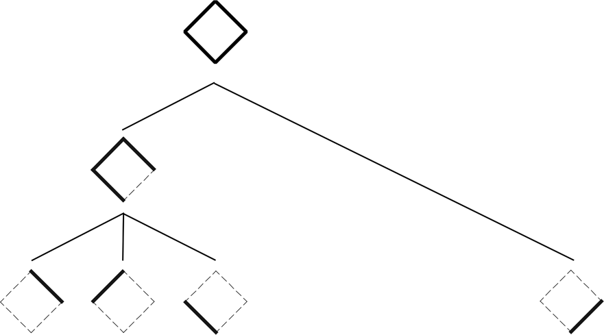
Discrete and bounded decompositions can be extended to other algebraic structures able to handle computational continuity and the recasting of computations with shapes into computations with atoms. Stiny (Reference Stiny1994) uses decompositions that are topologies and Boolean algebras. Krstic (Reference Krstic2010) uses hierarchies and topologies. Hierarchies have wide use in engineering. They describe designs and their components as sums of atoms. Hierarchies are ordered sets with unique paths between their elements, providing a global structure for shapes and presenting how parts are assembled. A shape is decomposed hierarchically by breaking it down into discrete parts and subparts. The result is a treelike structure with the whole shape at the top and the atoms at the bottom. The following diagram with a square presents a hierarchy containing two components: a Π and an I. The atoms of the hierarchy are four maximal lines (Fig. 7).
A hierarchy containing a Π-shape and an I-shape. The atoms are four lines.
In the four computations featured in this paper, topologies, Boolean algebras, and lattices are used to present algebras of decompositions with lines in the algebra U 12, based on applying a single identity. If B(α) denotes the set of all parts of a shape α, then the set B(α) is a sub-algebra of the algebra in which α is defined. The Boolean algebra B(α), which is closed under the symmetry group S(α) of α, is the maximal structure of shape α. The algebra B(α) is a proper subalgebra of Uij.
If B(x) is a Boolean algebra formed by the four maximal lines of a square, then the four lines are its base, and B(x) is a finite (16-element) Boolean algebra depicted in the preceding diagram. B(x) is a subalgebra of U 12 (Fig. 8).
The four maximal lines of a square form a Boolean algebra.

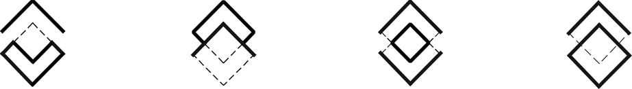
The topologies change as emergent shapes are presented in the course of a computation. When emergent shapes are acknowledged locally, novel forms are highlighted globally. In the example, the identity rule that recognizes squares applies to a shape including eight maximal lines to present three squares. One of them is emergent (Fig. 9).
The identity rule (left) applies to the shape (center) to present three squares. One of them is emergent (right).

Table 1 presents a shape C, the recognized shapes t(A) ≤ C, and their complements C − t(A). It also presents the closure structure of sub-shape t(A) associated with the parts of C. The closure of any sub-shape x of C is the smallest element of C containing x.
Complement and closure of sub-shape A in a shape C

The topology containing eight maximal lines provides 28 sub-shapes without recognizing the emergent square. The structure of a shape can be relativized to each of its parts (Krstic, Reference Krstic2005). Figure 10 presents a shape α, its decomposition A including eight maximal lines A, and shape β a small square, on the right which is part of shape α (β ≤ α).
Shape α (left), its decomposition A (center), and shape β (right).

Then β can be structured in decomposition B = {β • x | x ∈ A}. Decomposition B contains the product parts of β with decomposition A. In other words, structure B is the relativization of A to β. Table 2 presents the relativization of shape structure. The top row of Table 2 presents the initial decomposition of shape C, a set of eight lines. The left column includes the recognized sub-shapes β and γ. The shapes β ≤ C and γ ≤ C organize a structure B = {β • x | x ∈ C}, and Γ = {γ • x | x ∈ C}.
Relativization of the two decompositions for C
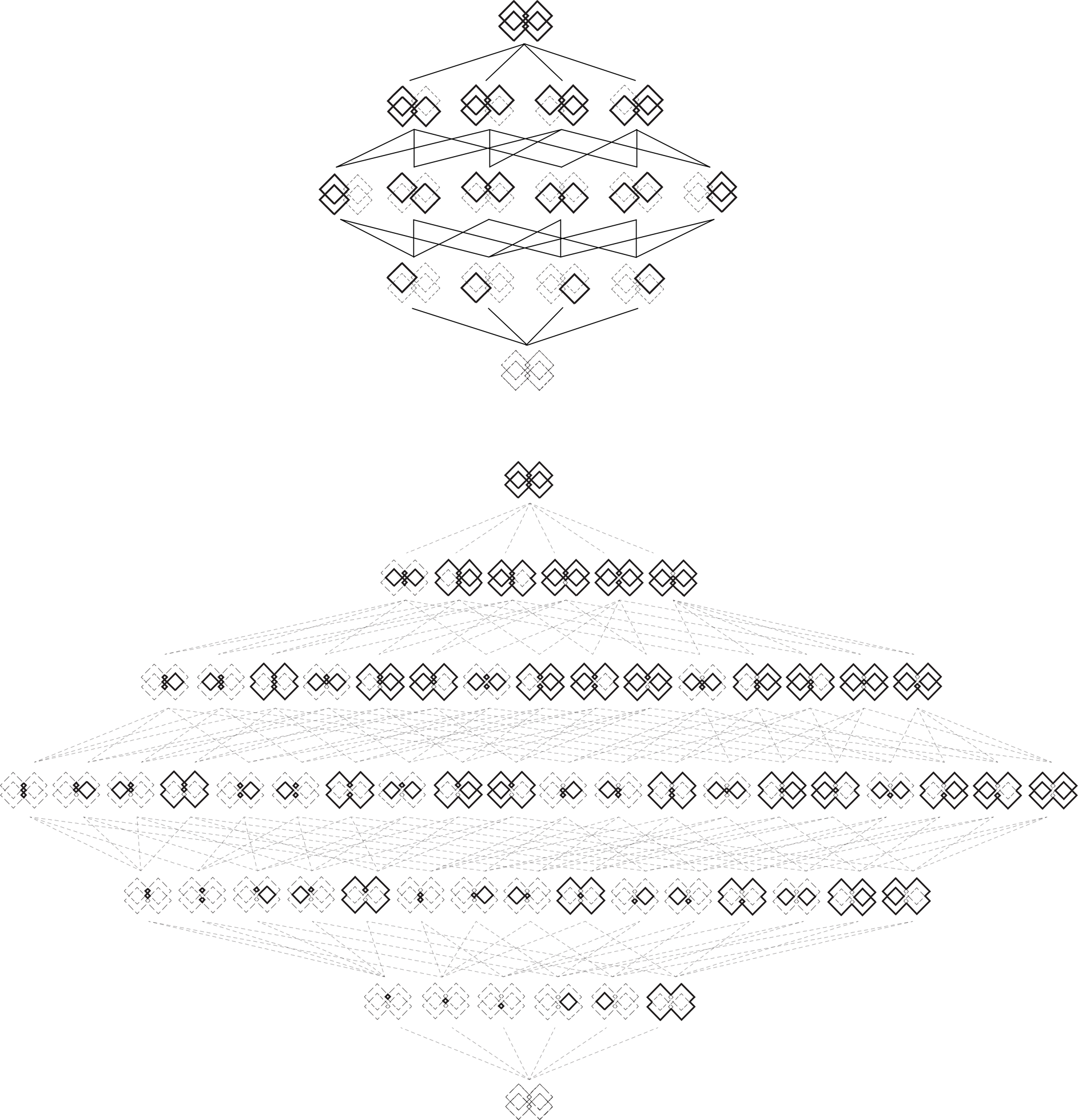
The following Table 3 illustrates the two different topologies representing the same shape based on Coleridge's Μethod: thesis (two equal squares, eight maximal lines) and antithesis (a small square and its complement). Their resolution comes in two hierarchical decompositions (Boolean algebras), which construct the topologies’ elements. The two hierarchical decompositions share a set of atoms, a discrete shape decomposition, which is the key to resolving their parts (synthesis). Drawing on a geometrical analogy originating in the Pythagoreans, Coleridge represents thesis and antithesis as the opposite poles of a line, while its midpoint represents their synthesis, “the indifference of the two poles.” In the graphical representation that follows, the two hierarchies share a set of atoms appearing on the axis of symmetry of the diagram.
The two hierarchical decompositions (thesis–antithesis) share a set of atoms, a discrete decomposition of the shape, which is the key to the resolution of their parts (synthesis)
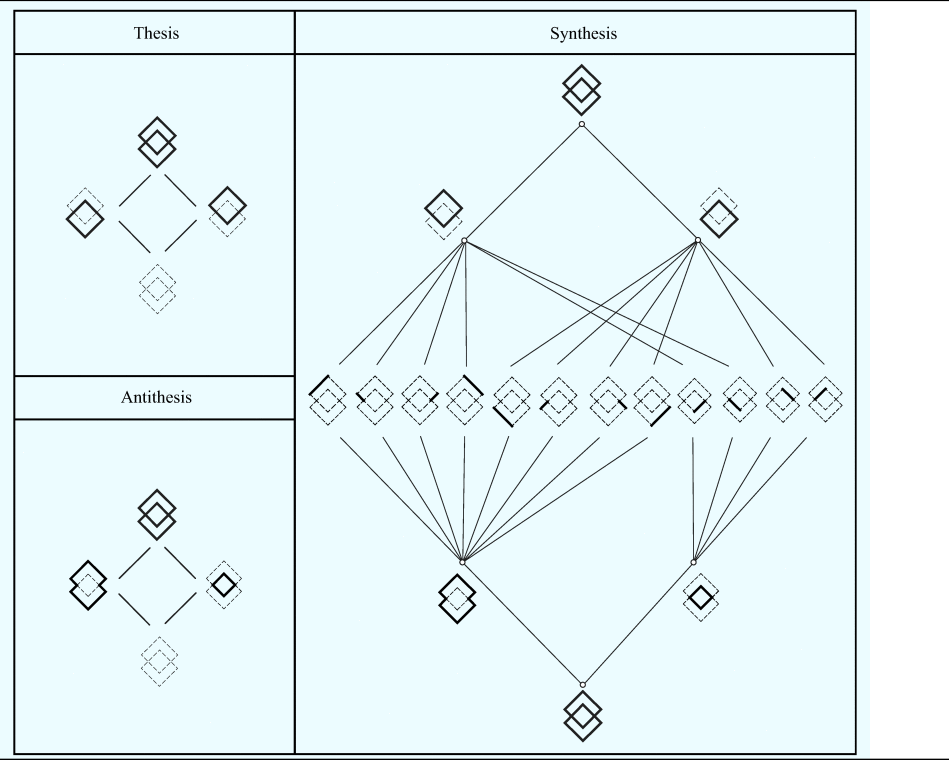
Coleridge's scheme supposes a union of several elements into a synthesis that is indifferent to these elements. Based on this method, multiple hierarchical decompositions for a shape can be resolved in sequence, two at a time. The shape itself turns out to be the synthesis of any hierarchical decompositions as it is indifferent to any particular one of these.
Six linear segments now describe the initial square, and two discrete decompositions describe the square. The two squares have different sizes and include four and six linear segments apiece (Fig. 11).
The small square (left) contains four lines, and the initial square (right) now contains six lines.
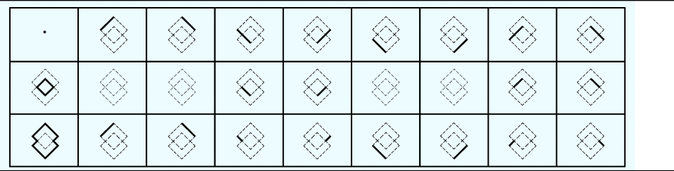
A topology and Boolean algebra, including the 212 permutations of the 12 atoms and the empty shape, exhaust the sub-shapes of C. Even with the very narrow objective of presenting all squares, new parts introduced in the topology and new sub-shapes are highlighted. These sub-shapes are highlighted globally as the parts of the square change locally. Examples of shapes in the topology of C are presented in Figure 12.
Examples of shapes that are highlighted in the topology of C.
It is worth noticing that since shape C determines a Boolean algebra, a non-empty sub-shape Δ of shape C (with Δ, C ∈ Uij) satisfies the algebraic conditions of an ideal (Table 4): (i) if x ≤ Δ and y ≤ Δ, then x + y ≤ Δ, and (ii) if x ≤ Δ and y ≤ x, then y ≤ Δ. Since the empty shape is part of every x, it is part of every Δ of C. Any proper sub-shape Δ of a shape C, with Δ ≤ C and Δ ≠ C, fulfills the algebraic conditions of a proper ideal. An algebra containing the empty shape as the only proper ideal is called simple. The Boolean algebra U 00 containing a single point fills the conditions of a simple algebra.
Sub-shapes, Boolean ideals and filters

Furthermore, a non-empty sub-shape Δ′ of shape C (with Δ′, C ∈ Uij) satisfies the algebraic conditions of a filter: (iii) if x′ ≤ Δ′ and y ≤ Δ′, then x′ • y′ ≤ Δ′; and (iv) if x′ ≤ Δ′ and x′ ≤ y′, then y′ ≤ Δ′. The Boolean structure of a filter is dual to that of an ideal (Table 4). The conditions (iii) and (iv) are obtained by (i) and (ii), by replacing sum, product, ≤, by product, sum, ≥. It follows that if Δ′ is a filter, then Δ is an ideal.
Given any sub-shape δ of a shape β (δ ≤ β) with δ, β ∈ U, and i, j ≠ 0, the intersection τ of all sub-shapes α of β containing δ (i.e., such that δ ≤ α) is itself a sub-shape of β that contains δ. There is at least one sub-shape of β containing δ, namely the shape β itself. Let shapes x and y be parts of the intersection τ, and z part of shape β. If α is any sub-shape of β containing δ, then x ≤ α and y ≤ α. Hence, the sum x + y ≤ α. Likewise, x • z ≤ α. Thus, x + y and x • z are in τ, and therefore, τ is a sub-shape of β, and also an ideal.
In any shape β ∈ U with i, j ≠ 0, a set δ of sub-shapes, or ideals, of β organizes an inclusion chain of sub-shapes in β if and only if, for any sub-shape α 1 and α 2 in δ it is either α 1 ≤ α 2 or α 2 ≤ α 1 that orders δ. The union of such an inclusion chain of sub-shapes is again a sub-shape of β.
Four compositions with squares
A copy of the shape is added (Fig. 13).
A copy of the shape (left) is added (right).

The added shape is translated twice to the left before being translated to the right and stopped (Fig. 14). This exemplary process corresponds to physically shifting the added shape over the existing one on a transparency. A designer pauses the translation at will, and the following four shape arrangements are picked for further examination.
The added shape is translated twice to the left, then to the right, and stops (right).

The translation of a transparency can be replicated by a Euclidean transformation t or by parametric rules. A Euclidean transformation t can be a smooth translation of the added shape first to the left and then to the right. To achieve the same result with rules, a parametric rule 1 can move the added shape to the left and a parametric rule 2 to the right. The same result can be achieved with a single parametric rule and appropriate (positive, negative) parametric values (Fig. 15).
Parametric rule 1 moves the added shape left. Parametric rule 2 moves it right.

When applying the parametric rule, the position of the translated shape in shape C′ = (C − t(g(A)) + t(g(B) is determined by the range of the parametric value assignment g, which is chosen to output a smooth translation. In both cases (Euclidean transformation or parametric rule), the pausing locations of the translation are unknown. The designer decides to pause based on visual criteria. Rule continuity is not a relevant design issue when the process begins because the four shape arrangements are not known in advance, they are picked during the process based on their appearance.
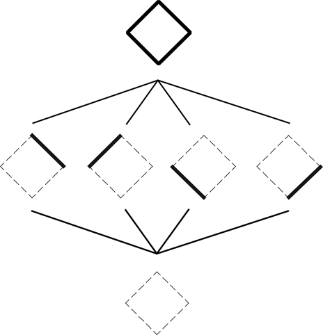
An identity A → A is used as an observation device to recognize all squares in the four produced arrangements (Fig. 16).
This identity rule is used as an observation device.

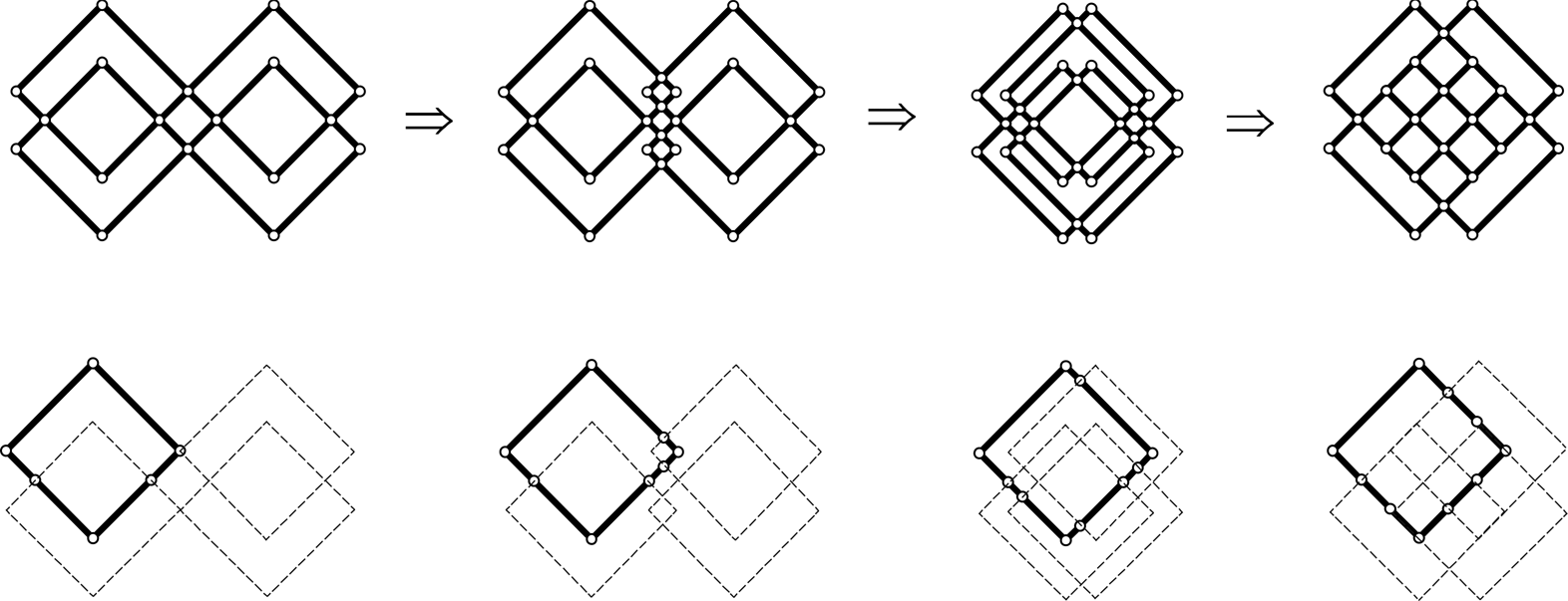
The four arrangements are selected out of numerous intermediate shape positions (Fig. 17). The identity rule constructs the topologies for the four shapes sequentially by reorganizing their parts one after another to recognize t(A) in C. The sum of the graphic material – lines in the algebra U 12 – used to construct the shapes remains unaltered in the computation. No lines are added or subtracted, and lines remain discrete in three of the four steps.
The four shape arrangements are selected out of innumerable others.

March (Reference March1996) mentions Lucretius’ parallel translation of atoms, “motion by which the generative bodies of matter give birth to various things.” A similar approach is adopted in this example. The translation of shapes, rather than atoms, can act on many shapes in parallel. The example is limited to two initial pairs of squares. A matching design scenario is the translation of a transparency with a drawing on top of another drawing to explore new arrangements. Beyond re-arrangement of existing shapes through translation, when two shapes intersect, new shapes emerge.
In the example, when the observer pauses the shape translation, the recognition of emergent squares becomes the primary objective. In a more realistic setting, one can imagine a designer distinguishing a variety of emergent shapes. The application of the identity rule locally revises the topologies of C1, C2, C3, and C4, highlighting different parts and sub-shapes. Their topology is changed to contain the recognized emergent shapes which are not in it by revisiting the products between old and new parts.
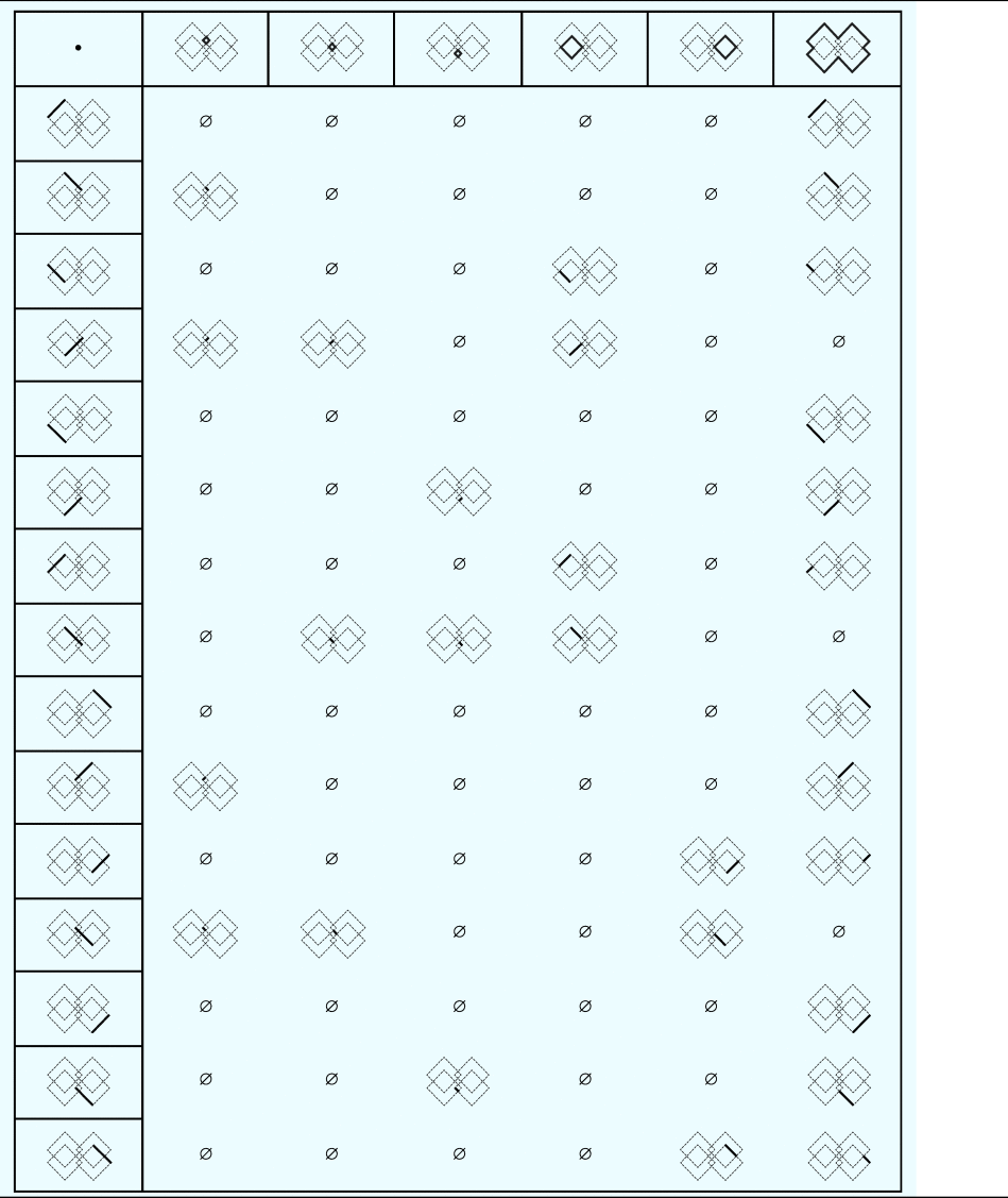
The following Table 5 provides an overview of the basis elements of the topologies for the four shapes based on applying the identity rule for squares. The discrete decompositions for squares, including all the required atoms to recognize emergent squares, are also included in Table 5.
Basis elements of discrete topologies, and atomic lines for squares
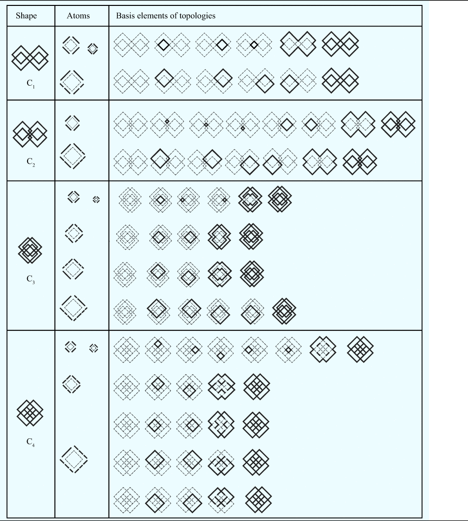
The first shape in Table 5, the shape C1, is an arrangement of 12 maximal lines. Our interest in recognizing squares yields a discrete decomposition of the shape containing 24 linear segments (Fig. 18).
The shape C1 contains 12 maximal lines (left). A discrete decomposition of 24 linear segments enables the recognition of all emergent squares (right).

Seven squares are recognized in the shape (Fig. 19). All squares are emergent if we consider the maximal lines as starting description. The squares are three when the symmetrical ones are removed.
Seven squares are recognized. They remain three when the symmetrical ones are removed.

The two topologies (Boolean algebras) for shape C1 (Table 5) are not conflicting (Fig. 20).
Two Boolean algebras for the shape C1.

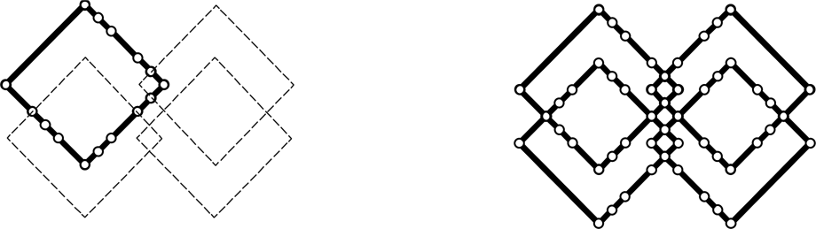
A topology for C1 is presented, recognizing all seven squares (Fig. 21). The analysis of six lines per large square yields a set of 24 atoms. The circles indicate the “joints” of the line segments, signifying that they are recast into indivisible elements (points).
Six lines per large square (left) and a set of 24 atoms for C1 (right).

Three discrete decompositions for squares are formed (Fig. 22). The smallest square contains four short lines. Two more squares of different sizes are recognized, containing four and six linear segments each. Six linear segments compose the initial large square.
Four short lines form the smaller square (left). Two more squares of different sizes are recognized (right), containing four and six linear segments.

A topology and Boolean algebra, including the 224 permutations of the atomic line segments and the empty shape, exhaust the sub-shapes of the shape. Examples of other shapes in the topology of C1 are presented in Figure 23.
Examples of other shapes in the topology of C1.

The second shape in Table 5, the shape C2, is an arrangement of 16 maximal lines. The recognition of squares yields a discrete decomposition containing 32 linear segments (Fig. 24).
The shape C2 includes 16 maximal lines (left). A discrete decomposition of 32 linear segments enables the recognition of all emergent squares (right).

Nine squares are identified in C2. They are presented in Figure 25 after the symmetrical ones are removed. Four of them are non-emergent (left), and five are emergent (right).
Nine squares are recognized in C2. They remain four when the symmetrical ones are removed.

As new topologies are established for C1, C2, C3, and C4, their structures are relativized, and new sub-shapes emerge as combinations of the new parts. An example is the relativization of two conflicting topologies (Boolean algebras) for shape C2 (Fig. 26).
Example of two conflicting Boolean algebras for C2.
Conflicting topologies are relativized in the usual manner by revisiting the products of their parts. This can involve tedious bookkeeping. The relativization of the above two topologies for shape C2 so that all nine squares are recognized is presented in Table 6. The emerging squares and their complement are relativized against the 16 maximal lines.
Relativization of parts for shape C2.
A new relativized topology for C2 is presented, recognizing all nine squares. The analysis of eight lines per initial square yields a set of 32 atoms for C2. Again, the circles indicate the “joints” of line segments (Fig. 27).
Eight lines per large square (left) and a set of 32 atoms for C2 (right).
The square now obtains three different discrete topologies in the global topology of C2, including four, four, and eight linear segments of various lengths. The eight linear segments composing the initial, largest, and square appear on the right (Fig. 28).
The square now obtains three discrete topologies in C2, including four, four (left), and eight linear segments (right) of various lengths.

A Boolean algebra, including the 232 permutations of these, exhausts all sub-shapes of C2. The newly adjusted topology permits the recognition of other shapes in it. Examples of shapes in the topology of C2 are presented in Figure 29.
Examples of other shapes in the topology of C2.

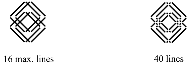
The third shape in Table 5, the shape C3, is an arrangement of 16 maximal lines. A discrete decomposition of the shape containing 40 lines is formed based on the identity (Fig. 30).
The shape C3 includes 16 maximal lines (left). A discrete decomposition of 40 linear segments enables the recognition of all emergent squares (right).
Eleven squares are identified in shape C3. Four of them are non-emergent and seven emergent. The squares are presented in Figure 31 after the symmetrical ones are removed.
Eleven squares are recognized in C3. They remain five if the symmetrical ones are removed. Four of them, like the one on the left, are non-emergent. Seven are emergent (right).

The four conflicting topologies (Boolean algebras) for C3 are presented next (Fig. 32).
Four Boolean algebras for the shape C3.

A new relativized global structure for C3 can be supplied, recognizing all 11 squares. It includes 40 linear segments. Ten linear segments form the initial largest square (Fig. 33).
Ten lines per large square (left) and a set of 40 atoms for C3 (right).

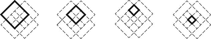
Specifically, the square now obtains five discrete topologies in the global topology of C3, including four, eight, eight, and ten linear segments (Fig. 34).
The square is now analyzed in five discrete decompositions, including four, eight, eight (left), and ten linear segments (right) of various lengths.

Forty atoms compose the shape C3. A topology, including the 240 permutations of these, exhausts its sub-shapes. Examples of shapes in this topology appear in Figure 35.
Examples of shapes in the topology of C3.

The fourth shape in Table 5, the shape C4, is an arrangement of 12 maximal lines. A discrete decomposition of the shape containing 34 lines is formed based on the identity (Fig. 36).
The shape C4 includes 12 maximal lines (left). A discrete decomposition of 34 linear segments enables the recognition of all emergent squares (right).

Thirteen squares are identified in the shape C4, which are all emergent. They are reduced to four if the symmetrical ones are neglected (Fig. 37).
Thirteen emergent squares and recognized in C4. They are reduced to four.
Five conflicting Boolean algebras are formed for C4 after applying the identity. A representative algebra appears in the diagram of Figure 38.
A representative Boolean algebra, out of five, for C4.

A relativized structure for C4 is formed after recognizing all 11 squares. Ten linear segments compose the initial, largest, square, and 34 line segments make the whole shape (Fig. 39).
Ten lines per initial square (left) and a set of 34 atoms for C4 (right).

An individual square now obtains four discrete topologies that are presented in Figure 40. They include four, four, eight, and ten linear segments of various lengths, respectively.
There are four discrete decompositions for the square in C4, including four, eight, eight (left), and ten lines (right) of various lengths.
A topology, including the 234 permutations of the 34 linear segments, exhausts the sub-shapes of C4. Other shapes in this topology that are produced as combinations of the emerging parts are presented in Figure 41.
Examples of shapes in the topology of C4.

The featured visual examples imitate the translation of a drawing on top of another drawing to explore shape arrangements. When two shapes intersect, new shapes can emerge and the topologies of C1, C2, C3, and C4 are relativized to include the necessary parts for the recognition of emergent squares. The goal of square recognition is realized by revisiting the products between old and new shape parts at each step and adjusting them accordingly.
Adjusting the topology of a shape based on a rule yields an interpretation of the shape structure as a whole. Parts can be included or excluded as needed, and combinations of parts can yield new sub-shapes that may have an aesthetic or another appeal. Going from unanalyzed to analyzed shapes and back is a practical design tool. However, things that we do effortlessly in visual design with shapes without tracking structural change become challenging when we aim to keep track of structural change. The progression of structure is implicit, and it is not visual. It is not easy to foresee the progression of the global structure after a rule is applied locally unless one deliberately examines the structure. Moreover, even in the most straightforward computations, it is not easy to envision the combinations of continuously changing parts or relativize a set of parts to another. Tracking parts and structure with sets can go quickly out of hand as counting and bookkeeping struggle to follow what the eye effortlessly perceives.
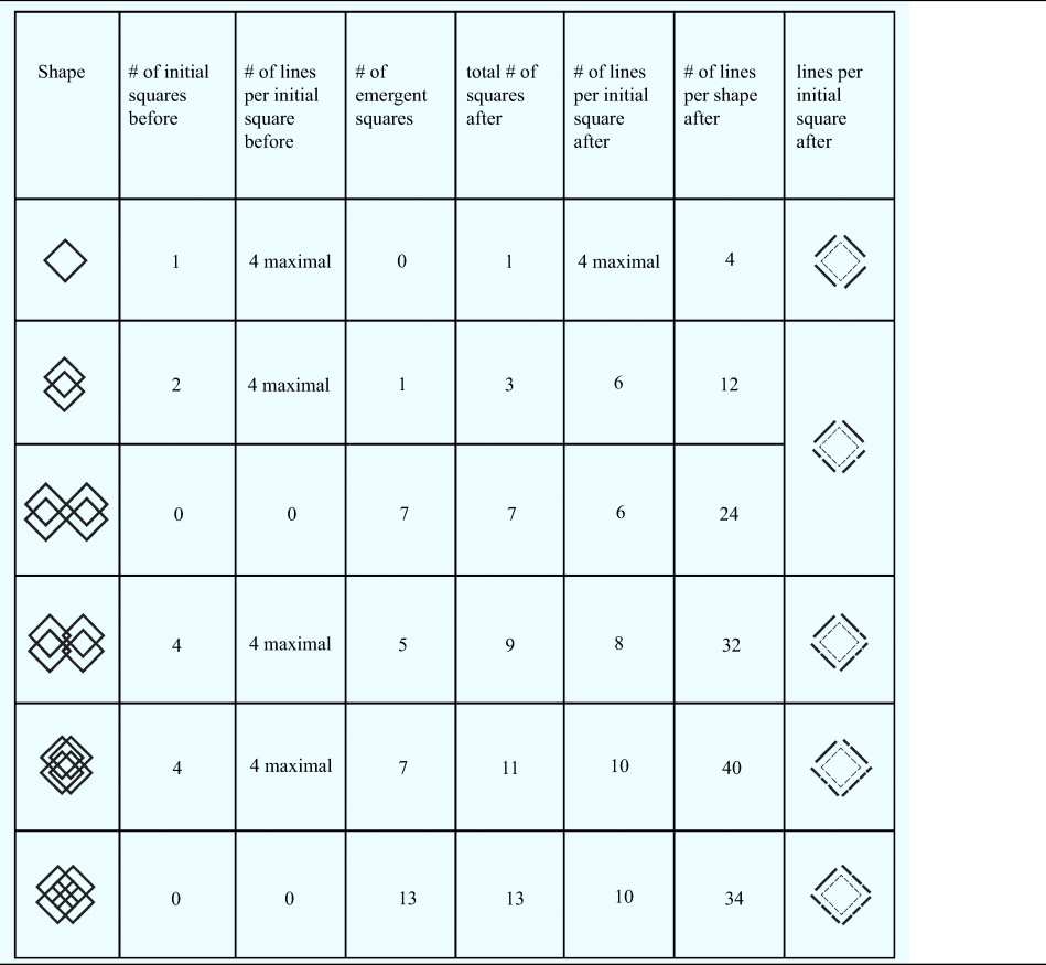
Table 7 summarizes the modifications in the number of squares and lines per square before and after adjusting the topologies to recognize squares at each step of the computation.
Counting lines and squares before and after adjusting the topologies
Topologies can be used to record and recall the generative history of a design in retrospect. The generative history is helpful when designers want to revisit the products or the steps of a design process. Retrospective analysis can serve evaluation purposes or establish a routine for generating a particular class of objects. The generative history is recorded in the rules and the shape decompositions differently. Rules are recursive but not mechanical; they follow what we see. Structures like hierarchies and Boolean algebras, on the other hand, lack organic unity; they capture combinations.
Rule continuity for C1, C2, C3, and C4 can be established recursively at the end. The topology is configured backward so that the application of the translation and the identity rule are continuous. Continuity provides a global kit of parts (point set) that works throughout without glitches, enabling the recognition of all squares. The parts in all four computations can now interlock in proper positions, like mechanical components with invariable joints (Fig. 42).
The interlocking positions or “joints” for C1, C2, C3, and C4. The joints for the initial square in each computation are demonstrated in parallel.
The shape joints signifying specific interlocking positions for the entire computation course demonstrate a typical set-theoretic (mechanical) sum in which things remain discrete, each with an invariant identity. They emphasize the difference of a visual (organic) sum in which all joints disappear via the reduction rules. Even though the topologies we are concerned with have finite parts, the number of nodes can be overwhelming.
Furthermore, as Jowers et al. (Reference Jowers, Earl and Stiny2019) indicate, new parts “may decompose the shape into infinitesimal parts for which it is impossible to make provision.” Hence, it is better to adopt a shape perspective, “choosing/constructing parts, transforming those parts, fusing them back together while revealing new parts.”
Discussion
Designers are concerned with how forms are understood by their parts and how parts fit to serve various purposes. Resolving the form and structure of physical objects means establishing proper relationships of parts to parts and parts to wholes. We seek technical, aesthetic, semantic, or other criteria and rules to judge these relationships essential to composition in every design judgment. Determining the parts and the rules of their assembly leads to a grammar of form, which helps us get the sense of detail and compose large structures by assembling their parts and fitting them into their context. It has a central role in mastering good results in art, design, and engineering. However, to master something, you need to see it first.
The polymath Leon Battista Alberti argues that art relies on observation and chance. In his book On Sculpture Alberti (Reference Alberti and Grayson1443) notes: “artists occasionally observed in a tree-trunk or clod of earth and other similar inanimate objects certain outlines in which, with slight alterations something very similar to the real faces of Nature was represented.” Then, Alberti continues artists began to complete the likeness “by diligently observing and studying such things” and “adding, subtracting or supplying what was missing.” Another renowned designer and inventor, Leonardo Da Vinci, revealed a similar method for painting his frescoes (Richter Reference Richter1939): “looking attentively at a wall spotted with stains … to discover a resemblance to various compositions and an endless variety of objects that appear confusedly but can be reduced to any well-drawn form one chooses to imagine.” Often accused of staring for hours at the wall, constantly reworking his paintings, and being helplessly slow in execution, Da Vinci was notorious for never finishing a work. He spent more than three years painting the Last Supper and more than five years working on the Mona Lisa without never finishing.
The techniques of Alberti and Leonardo highlight the vital role of perpetual observation in art and design. However, they come at odds with our current experience of CAD systems, Augmented Reality, and Virtual Reality, where an invention is approached as a matter of computational complexity, speedy generation of large solution spaces, and virtual augmentation. Gazing at tree trunks, clods of earth or the bare wall sounds like the most simplistic and unproductive thing to do. Nevertheless, we have not yet seen any visual masterpieces coming out of AI, VR, or automated design production.
John von Neumann (Reference von Neumann and Burks1940) raises concerns on how knowledge representation captures our visual experience. He suggests that even a simple shape like a triangle can never acquire a permanent representation as a visual analogy, no matter how hard one tries or how much data one has. Von Neumann concludes that resolving shape structure is idiosyncratic; it is like taking a Rorschach test; it reveals one's character. Perhaps von Neumann's psychological approach to shape bears some humorous undertones, considering that he delivered his speech in an audience of distinguished mathematicians, logicians, and researchers of early computer science, at the Hixon Symposium. However, von Neumann's brief comment introduces a new domain of computational inquiry, not foreign to everyday experience and distinct from information processing. In this new domain, visual perception and personal interpretation have priority over logical representation.
Our drafting experience confirms this. Drawings synthesize visual elements without a built-in ordering to suggest a permanent logical structure. It takes design students more than five years of copious design training to assimilate the standard underlying conventions of depicting any structure at all. The shapes presented in a drawing do not fulfill knowledge representation criteria; their primary appeal is their appearance, which provides visual material for exploring structure. Resolving shape structure and relations of parts to parts and parts to wholes is vital. Drawings begin with sketchy lines, then tracing paper is introduced to enable copying and embedding. At first, maximal lines offer an efficient and economical way to handle shapes; soon, seeing intervenes, and new arrangements of the graphic material into meaningful parts are introduced.
Lionel March (Reference March1996) contrasts the macro-behavior of atomic systems like cellular automata and fractals against shapes to compare their productive potential. Both worlds exhibit emergent properties, however, of different kinds. In cellular automata and fractals, rules apply globally and in parallel, while in computations with shapes, rules apply locally and step by step. Emergence in atomic systems depends on the prescribed encoding of the atoms’ macro-behavior and the system's global order rather than observation of local interaction. Shuffling atoms based on syntactic rules can yield unexpected patterns mechanically. On the other hand, emergence in nonatomic shape systems does not require a prescribed global order, like a grid. Local spatial relations determine the global generative possibilities of the system. Shape rules apply locally when a sub-shape is selected, and any two intersecting shapes can generate other emergent shapes. In this way, the interaction of shapes is organic, giving rise to spontaneous creation or destruction, in a process in which seeing is of primary constructive importance.
Similarly, the four computations with squares presented in this paper emphasize how the visual selection of parts affects the productive potential in a rudimentary design system. To this end, translating squares on top of one another resembles translating two drawings using tracing paper. In both cases, new possibilities for distinguishing parts and wholes emerge. A simple observation goal was set: the recognition of squares. This choice has significant local and global constructive implications because selecting a part provides structure and divides the shape into subparts. Naturally, shapes of higher than zero dimension can have infinitely many finite decompositions that can obtain structures like topologies, hierarchies, Boolean algebras, which enable us to treat them algebraically.
Topologies are structurally informative because they uniquely depict a global view of a shape by representing each of its parts. The members of a topology are the parts of the shape the topology recognizes. Because a topology includes the whole shape and the empty shape, it provides a context for comparing parts and their combinations, making alternative structures comparable. Topologies are also semantically indicative since they offer a global interpretation of unanalyzed shapes into meaningful entities by presenting desirable parts and combinations. Producing alternative part combinations facilitates the exploration of structure, which is essential in the creative stages of design.
In the featured example, the topology of each produced shape is modified to contain the necessary parts to recognize emergent squares. This goal is achieved by revisiting the products between old and new parts. From a design point of view, modifying the topology of a shape offers a design alternative as new subparts emerge. When specific parts change through observation, other emergent shapes are highlighted in the topology. Modifying how we select local parts modifies how we see and analyze the global whole. Local observation leads to a global structure and fresh design possibilities. More action follows in the typical design scenario, as shapes return in their unanalyzed condition before a rule imposes structure again and a new topology is supplied. Analysis and synthesis are tightly interconnected in a process that moves from appearance to structure and back.
Hence, a drawing's primary purpose is to construct a design rather than communicate structural information. In this process, it is critical to synthesize conflicting structures. Stiny (Reference Stiny2022) uses the embed-fuse cycle and Boolean algebra and topology to introduce, represent, and synthesize structures in shape grammars. Interestingly, in a similar fashion, the English poet Samuel Taylor Coleridge draws from the Pythagoreans and the German dialectic tradition to synthesize two opposing descriptions, a thesis and an antithesis in art and poetry. A notable characteristic of Coleridge's Method is that it aims to reach higher degrees of synthesis through transition, not by eliminating polarities but by synthesizing them. While Coleridge proposes the Method to enlighten the transitions of organic things of nature, art, and poetry, the Method is suitable for design too. Technically, in shape grammars, the transition can mean relativizing the topology of a shape (Krstic, Reference Krstic2005) to allow two opposing descriptions, a thesis and an antithesis, to coexist in a single shape. Stiny (Reference Stiny2022) observes that since every shape from lines, planes, or solids synthesizes innumerable structures, it is indifferent to all descriptions offering material for infinite creative transitions.
Today, design is the most popular word in all branches of engineering. Everybody designs! Posing and answering retrospective questions, like: “What if I had acted differently? What if I were to do things differently?” is the typical mode of design inquiry. Hence, dynamic description that allows interrogation and transition is preferable to fixed data. Judea Pearl (Reference Pearl and Brockman2019) writes eloquently on the need for transparent, causal representations, in science and engineering, instead of opaque data systems. He concludes that: “Data science is a science only to the extent that it facilitates the interpretation of data—a two-body problem, connecting data to reality. Data alone are hardly a science, no matter how “big” they get and how skillfully they are manipulated.” Transparency, effortless reinterpretation of counterfactual design scenarios are highly valued in design and engineering. It turns out that computations with shapes, shape rules and decompositions fulfill these needs admirably. Shape decompositions are conveniently finite, offering an economical medium to explore and synthesize many views, and shape rules – embedding and fusing – are the basis of a seamless transition from one view to another.
Having a simultaneous view of both worlds, unstructured and structured, is the reasonable thing to do. Going from appearance to structure and back is an original design tool. The succession of structures remains implicit. It is not visual, and it is not easy to foresee. Documenting the applied rules and recasting shapes to topologies or Boolean algebras helps preserve the generative history and provides a superb medium for comparison and evaluation. However, what we do effortlessly in visual computation with shape rules without tracking structural change could become computationally challenging when we do it via representations that track all structural change. Shape rules and decompositions differ in nature. Shape rules have observational power because they track what we see each time we apply them. Decompositions serve bookkeeping by tracking parts and combinations. Nonetheless, as this paper exhibits, the bookkeeping of parts is tedious.
Finally, design synthesis advances leisurely instead of abruptly, which is a characteristic of the automated mode of production. In this slow visual process, transparency is indispensable. Adopting design automation in exchange for speed and efficiency leads to a different design experience that conceals its limitations. Automated, opaque processes often supply many suitable design “answers” or “options” but tactfully remove the seeing/thinking from the process. Perhaps some of the standard problems in engineering are a good fit for such speedy efficiency. However, creative design does not have much to gain from knowledge representation and speedy automation.
Furthermore, sloppy, visual description with which the designer might feel free to identify alternative modes of interpretation can often be more constructive than meticulously polished and fixed knowledge representation. In general, the more determined in a description, the more rigid rules intervene in its interpretation, and the more one must adjust action to given operation routines. The less determined these details are, the more direct the way of interacting with a description is, and the fewer fixed rules intervene. Recently a new generation of shape interpreters, like the Shape Machine presented in Economou et al. (Reference Economou, Hong, Ligler and Park2019), promise to “fundamentally redefine the way shapes are represented, indexed, queried and operated upon” and resolve many of these long-overdue issues.
Sotirios D. Kotsopoulos, is a researcher, designer, and educator in computational design, focusing on shape grammars, formal systems, and morphology. He examines constructive associations of form, structure, and performance and explores the nature of collaboration among design disciplines. Sotirios holds a PhD in Design & Computation from MIT. He is a researcher at the MIT Media Lab and an Associate Professor of computational design at the School of Architecture of the National Technical University of Athens (NTUA).


 Open access