


1 Introduction
1.1 Definition of the groups
We denote by $\Sigma _{g,1}$
the orientable surface of genus g with one boundary component, and by
$\Sigma _{g,1}$
the orientable surface of genus g with one boundary component, and by $\Gamma _{g,1}=\pi _0(\operatorname {Diff}_{\partial }(\Sigma _{g,1}))$
its mapping class group, defined to be the group of isotopy classes of diffeomorphisms of
$\Gamma _{g,1}=\pi _0(\operatorname {Diff}_{\partial }(\Sigma _{g,1}))$
its mapping class group, defined to be the group of isotopy classes of diffeomorphisms of $\Sigma _{g,1}$
fixing pointwise a neighbourhood of its boundary. We will define the spin mapping class groups using the approach of [Reference Harer8], which is based on the notion of quadratic refinements.
$\Sigma _{g,1}$
fixing pointwise a neighbourhood of its boundary. We will define the spin mapping class groups using the approach of [Reference Harer8], which is based on the notion of quadratic refinements.
Given an integer-valued skew-symmetric bilinear form $(M,\lambda )$
on a finitely generated free
$(M,\lambda )$
on a finitely generated free $\mathbb {Z}$
-module, a quadratic refinement is a function
$\mathbb {Z}$
-module, a quadratic refinement is a function $q: M \rightarrow \mathbb {Z}/2$
such that
$q: M \rightarrow \mathbb {Z}/2$
such that $q(x+y) \equiv q(x)+q(y)+ \lambda (x,y) (\mod 2)$
for all
$q(x+y) \equiv q(x)+q(y)+ \lambda (x,y) (\mod 2)$
for all $x,y \in M$
. There are
$x,y \in M$
. There are $2^{\operatorname {rk}(M)}$
quadratic refinements since a quadratic refinement is uniquely determined by its values on a basis of M, and any set of values is possible.
$2^{\operatorname {rk}(M)}$
quadratic refinements since a quadratic refinement is uniquely determined by its values on a basis of M, and any set of values is possible.
The set of quadratic refinements of $(H_1(\Sigma _{g,1};\mathbb {Z}),\cdot )$
has a right
$(H_1(\Sigma _{g,1};\mathbb {Z}),\cdot )$
has a right $\Gamma _{g,1}$
-action by precomposition. By [Reference Johnson9, Corollary 2] this action has precisely two orbits for
$\Gamma _{g,1}$
-action by precomposition. By [Reference Johnson9, Corollary 2] this action has precisely two orbits for $g \geq 1$
, distinguished by the Arf invariant, which is a
$g \geq 1$
, distinguished by the Arf invariant, which is a $\mathbb {Z}/2$
-valued function on the set of quadratic refinements, see Definition 6.1. For
$\mathbb {Z}/2$
-valued function on the set of quadratic refinements, see Definition 6.1. For $\epsilon \in \{0,1\}$
we will denote by
$\epsilon \in \{0,1\}$
we will denote by $\Gamma _{g,1}^{1/2}[\epsilon ]:= \operatorname {Stab}_{\Gamma _{g,1}}(q)$
where q is a choice of quadratic refinement of Arf invariant
$\Gamma _{g,1}^{1/2}[\epsilon ]:= \operatorname {Stab}_{\Gamma _{g,1}}(q)$
where q is a choice of quadratic refinement of Arf invariant $\epsilon $
, and call this the spin mapping class group in genus g and Arf invariant
$\epsilon $
, and call this the spin mapping class group in genus g and Arf invariant $\epsilon $
. These groups are of importance as their classifying spaces are the moduli spaces of spin surfaces with one boundary component by [Reference Randal-Williams17, Section 2] defined in geometric terms using tangential structures. In particular, the study of their (co)homology is the study of characteristic classes of the corresponding type of bundles. (As an aside note let us mention that notation
$\epsilon $
. These groups are of importance as their classifying spaces are the moduli spaces of spin surfaces with one boundary component by [Reference Randal-Williams17, Section 2] defined in geometric terms using tangential structures. In particular, the study of their (co)homology is the study of characteristic classes of the corresponding type of bundles. (As an aside note let us mention that notation $\Gamma ^{1/2}$
to denote spin mapping class groups comes from the geometric idea that a spin tangential structure is essentially a choice of a square root for the tangent bundle.)
$\Gamma ^{1/2}$
to denote spin mapping class groups comes from the geometric idea that a spin tangential structure is essentially a choice of a square root for the tangent bundle.)
Similarly, for $g \geq 1$
the group
$g \geq 1$
the group $Sp_{2g}(\mathbb {Z})$
acts on the set of quadratic refinements of the standard symplectic form
$Sp_{2g}(\mathbb {Z})$
acts on the set of quadratic refinements of the standard symplectic form $(\mathbb {Z}^{2g},\Omega _g)$
with precisely two orbits, also distinguished by the Arf invariant. Thus, for
$(\mathbb {Z}^{2g},\Omega _g)$
with precisely two orbits, also distinguished by the Arf invariant. Thus, for $\epsilon \in \{0,1\}$
we can define the quadratic symplectic group in genus g and Arf invariant
$\epsilon \in \{0,1\}$
we can define the quadratic symplectic group in genus g and Arf invariant $\epsilon $
to be
$\epsilon $
to be $Sp_{2g}^{\epsilon }(\mathbb {Z}):= \operatorname {Stab}_{Sp_{2g}(\mathbb {Z})}(q)$
for a fixed quadratic refinement q of Arf invariant
$Sp_{2g}^{\epsilon }(\mathbb {Z}):= \operatorname {Stab}_{Sp_{2g}(\mathbb {Z})}(q)$
for a fixed quadratic refinement q of Arf invariant $\epsilon $
. The groups
$\epsilon $
. The groups $Sp_{2g}^{0}(\mathbb {Z})$
have appeared in the literature under the name of theta subgroups of the symplectic groups, and sometimes are denoted by
$Sp_{2g}^{0}(\mathbb {Z})$
have appeared in the literature under the name of theta subgroups of the symplectic groups, and sometimes are denoted by $Sp_{2g}^{q}(\mathbb {Z})$
, and they are of importance in number theory, see [Reference Lu15] for example. These groups are also relevant in the study of manifolds, as in [Reference Kupers and Randal-Williams14, Section 4], since they represent automorphisms of homology groups of manifolds that can be realized by automorphisms of the manifolds. The groups
$Sp_{2g}^{q}(\mathbb {Z})$
, and they are of importance in number theory, see [Reference Lu15] for example. These groups are also relevant in the study of manifolds, as in [Reference Kupers and Randal-Williams14, Section 4], since they represent automorphisms of homology groups of manifolds that can be realized by automorphisms of the manifolds. The groups $Sp_{2g}^{1}(\mathbb {Z})$
are less common but have appeared recently in the study of manifolds in [Reference Kupers and Randal-Williams14, Section 4], where they are denoted by
$Sp_{2g}^{1}(\mathbb {Z})$
are less common but have appeared recently in the study of manifolds in [Reference Kupers and Randal-Williams14, Section 4], where they are denoted by $Sp_{2g}^{a}(\mathbb {Z})$
. However, as we will see in Section 5.1, one of the novelties of this paper is the idea that even if one is only interested in studying the groups
$Sp_{2g}^{a}(\mathbb {Z})$
. However, as we will see in Section 5.1, one of the novelties of this paper is the idea that even if one is only interested in studying the groups $Sp_{2g}^0(\mathbb {Z})$
one should also introduce the other family,
$Sp_{2g}^0(\mathbb {Z})$
one should also introduce the other family, $Sp_{2g}^1(\mathbb {Z})$
, and study both simultaneously.
$Sp_{2g}^1(\mathbb {Z})$
, and study both simultaneously.
1.2 Statement of results
Before stating the results let us recall what stabilization maps mean in this context. We begin by fixing quadratic refinements $q_0,q_1$
of
$q_0,q_1$
of $(H_1(\Sigma _{1,1};\mathbb {Z}),\cdot ) \cong (\mathbb {Z}^2,\Omega _1)$
of Arf invariants
$(H_1(\Sigma _{1,1};\mathbb {Z}),\cdot ) \cong (\mathbb {Z}^2,\Omega _1)$
of Arf invariants $0,1$
respectively. Then, given any quadratic refinement q of
$0,1$
respectively. Then, given any quadratic refinement q of $(H_1(\Sigma _{g-1,1};\mathbb {Z}),\cdot ) \cong (\mathbb {Z}^{2(g-1)},\Omega _{g-1})$
, we get a quadratic refinement
$(H_1(\Sigma _{g-1,1};\mathbb {Z}),\cdot ) \cong (\mathbb {Z}^{2(g-1)},\Omega _{g-1})$
, we get a quadratic refinement $q \oplus q_{\epsilon }$
of
$q \oplus q_{\epsilon }$
of $(H_1(\Sigma _{g,1};\mathbb {Z}),\cdot ) \cong (\mathbb {Z}^{2g},\Omega _{g})$
. Moreover, the Arf invariant is additive, see Definition 6.1, so
$(H_1(\Sigma _{g,1};\mathbb {Z}),\cdot ) \cong (\mathbb {Z}^{2g},\Omega _{g})$
. Moreover, the Arf invariant is additive, see Definition 6.1, so $\operatorname {Arf}(q\oplus q_{\epsilon })=\operatorname {Arf}(q)+\epsilon $
.
$\operatorname {Arf}(q\oplus q_{\epsilon })=\operatorname {Arf}(q)+\epsilon $
.
Thus, using the inclusions $\Gamma _{g-1,1} \subset \Gamma _{g,1}$
and
$\Gamma _{g-1,1} \subset \Gamma _{g,1}$
and $Sp_{2(g-1)}(\mathbb {Z}) \subset Sp_{2g}(\mathbb {Z})$
we get stabilization maps
$Sp_{2(g-1)}(\mathbb {Z}) \subset Sp_{2g}(\mathbb {Z})$
we get stabilization maps
 $$ \begin{align*}\Gamma_{g-1,1}^{1/2}[\delta-\epsilon] \rightarrow \Gamma_{g,1}^{1/2}[\delta]\end{align*} $$
and
 $$ \begin{align*}Sp_{2(g-1)}^{\delta-\epsilon}(\mathbb{Z}) \rightarrow Sp_{2g}^{\delta}(\mathbb{Z}).\end{align*} $$
The goal of this paper is to study homological stability with respect to these stabilization maps. Before moving to the results observe that additivity of the Arf invariant under direct (pointwise) sum of quadratic refinements also allows us to define products
 $$ \begin{align*}\Gamma_{g,1}^{1/2}[\epsilon] \times \Gamma_{g',1}^{1/2}[\epsilon'] \rightarrow \Gamma_{g+g',1}^{1/2}[\epsilon+\epsilon']\end{align*} $$
and
 $$ \begin{align*}Sp_{2g}^{\epsilon}(\mathbb{Z}) \times Sp_{2g'}^{\epsilon'}(\mathbb{Z})\rightarrow Sp_{2(g+g')}^{\epsilon+\epsilon'}(\mathbb{Z})\end{align*} $$
which contain the stabilization maps as particular cases.
It is known since [Reference Harer8, Theorem 3.1] that spin mapping class groups satisfy homological stability in the range $d \lesssim g/4$
, that is, of the form
$d \lesssim g/4$
, that is, of the form $d \le g/4-C$
for some constant C, and their stable homology can be understood by [Reference Galatius4, Section 1]. Thus, improvements in the stability range are important as they lead to new homology computations, hence to new characteristic classes. In this direction, the previously known best bounds can be found in [Reference Randal-Williams17, Theorem 2.14], where a range of the form
$d \le g/4-C$
for some constant C, and their stable homology can be understood by [Reference Galatius4, Section 1]. Thus, improvements in the stability range are important as they lead to new homology computations, hence to new characteristic classes. In this direction, the previously known best bounds can be found in [Reference Randal-Williams17, Theorem 2.14], where a range of the form $d \lesssim 2g/5$
was shown. The first main result of this paper improves the known stability range.
$d \lesssim 2g/5$
was shown. The first main result of this paper improves the known stability range.
Theorem A. Consider the stabilization map
then:
-
(i) If
 it is surjective for
$2d \leq g-2$
and an isomorphism for
$2d \leq g-4$
.
it is surjective for
$2d \leq g-2$
and an isomorphism for
$2d \leq g-4$
. -
(ii) If
it is surjective for
$3d \leq 2g-4$
and an isomorphism for
$3d \leq 2g-7$
.


Moreover, there is a homology class $\theta \in H_2(\Gamma _{4,1}^{1/2}[0];\operatorname {\mathbb {F}_2})$
such that
$\theta \in H_2(\Gamma _{4,1}^{1/2}[0];\operatorname {\mathbb {F}_2})$
such that
 $$ \begin{align*}\theta \cdot-: H_{d-2}(\Gamma_{g-4,1}^{1/2}[\delta],\Gamma_{g-5,1}^{1/2}[\delta-\epsilon];\operatorname{\mathbb{F}_2}) \rightarrow H_d(\Gamma_{g,1}^{1/2}[\delta],\Gamma_{g-1,1}^{1/2}[\delta-\epsilon];\operatorname{\mathbb{F}_2})\end{align*} $$
is surjective for $3d \leq 2g-5$
and an isomorphism for
$3d \leq 2g-5$
and an isomorphism for $3d \leq 2g-8$
.
$3d \leq 2g-8$
.
Moreover, the result with $\mathbb {Z}[1/2]$
-coefficients is optimal (up to possibly a better constant term) by Lemma 7.2, and in particular the ‘slope
$\mathbb {Z}[1/2]$
-coefficients is optimal (up to possibly a better constant term) by Lemma 7.2, and in particular the ‘slope $2/3$
’ cannot be improved as in the case of the usual mapping class groups, see [Reference Galatius, Kupers and Randal-Williams6]. The last part of the theorem is an example of secondary homological stability, which means that it gives a range in which the defects of homological stability are themselves stable. By Corollary 4.4, a consequence is that the
$2/3$
’ cannot be improved as in the case of the usual mapping class groups, see [Reference Galatius, Kupers and Randal-Williams6]. The last part of the theorem is an example of secondary homological stability, which means that it gives a range in which the defects of homological stability are themselves stable. By Corollary 4.4, a consequence is that the $\operatorname {\mathbb {F}_2}$
-homology satisfies a
$\operatorname {\mathbb {F}_2}$
-homology satisfies a $2/3$
slope stability if and only if
$2/3$
slope stability if and only if $\theta ^3$
destabilizes by
$\theta ^3$
destabilizes by $\sigma _{\epsilon }$
; and otherwise the slope
$\sigma _{\epsilon }$
; and otherwise the slope $1/2$
of part (i) would be optimal with
$1/2$
of part (i) would be optimal with $\operatorname {\mathbb {F}_2}$
-coefficients, and hence integrally. We do not know which of these two alternatives holds. Finally we remark that the class
$\operatorname {\mathbb {F}_2}$
-coefficients, and hence integrally. We do not know which of these two alternatives holds. Finally we remark that the class $\theta $
is not uniquely defined, see Remarks 4.3 and 4.5, but its indeterminacy is small and the statement above holds for any such choice of
$\theta $
is not uniquely defined, see Remarks 4.3 and 4.5, but its indeterminacy is small and the statement above holds for any such choice of $\theta $
.
$\theta $
.
The second main result is about homological stability of quadratic symplectic groups.
Theorem B. Consider the stabilization map
then:
-
(i) If
it is surjective for
$2d \leq g-2$
and an isomorphism for
$2d \leq g-4$
. -
(ii) If
it is surjective for
$3d \leq 2g-4$
and an isomorphism for
$3d \leq 2g-7$
.


Moreover, there is a homology class $\theta \in H_2(Sp_8^0(\mathbb {Z});\operatorname {\mathbb {F}_2})$
such that
$\theta \in H_2(Sp_8^0(\mathbb {Z});\operatorname {\mathbb {F}_2})$
such that
 $$ \begin{align*}\theta \cdot-: H_{d-2}(Sp_{2(g-4)}^{\delta}(\mathbb{Z}),Sp_{2(g-5)}^{\delta-\epsilon}(\mathbb{Z});\operatorname{\mathbb{F}_2}) \rightarrow H_d(Sp_{2g}^{\delta}(\mathbb{Z}),Sp_{2(g-1)}^{\delta-\epsilon}(\mathbb{Z});\operatorname{\mathbb{F}_2})\end{align*} $$
is surjective for $3d \leq 2g-5$
and an isomorphism for
$3d \leq 2g-5$
and an isomorphism for $3d \leq 2g-8$
.
$3d \leq 2g-8$
.
Some results were previously known about homological stability of quadratic symplectic groups. In particular, [Reference Friedrich3, Theorem 5.2] and [Reference Charney2] already gave a stability result of the form $d \lesssim g/2$
following different techniques. However, the improvement to
$d \lesssim g/2$
following different techniques. However, the improvement to $d \lesssim 2g/3$
in part (ii) of the above theorem is new. As before, the last part is a secondary stability result which implies that either the
$d \lesssim 2g/3$
in part (ii) of the above theorem is new. As before, the last part is a secondary stability result which implies that either the $\operatorname {\mathbb {F}_2}$
-homology also has slope
$\operatorname {\mathbb {F}_2}$
-homology also has slope $2/3$
stability (if
$2/3$
stability (if $\theta ^3$
destabilizes) or the optimal slope of the
$\theta ^3$
destabilizes) or the optimal slope of the $\operatorname {\mathbb {F}_2}$
-homology is
$\operatorname {\mathbb {F}_2}$
-homology is $1/2$
(otherwise). The class
$1/2$
(otherwise). The class $\theta $
is again not well-defined but its indeterminacy is understood by Remarks 4.3 and 4.5.
$\theta $
is again not well-defined but its indeterminacy is understood by Remarks 4.3 and 4.5.
We will prove Theorems A and B using the technique of cellular $E_k$
-algebras developed in [Reference Galatius, Kupers and Randal-Williams5], and in particular we will follow the overall strategy of [Reference Galatius, Kupers and Randal-Williams6] where this approach is applied to homological stability of mapping class groups of surfaces. However, as we will comment below some interesting novelties appear in our case.
$E_k$
-algebras developed in [Reference Galatius, Kupers and Randal-Williams5], and in particular we will follow the overall strategy of [Reference Galatius, Kupers and Randal-Williams6] where this approach is applied to homological stability of mapping class groups of surfaces. However, as we will comment below some interesting novelties appear in our case.
The basic idea is to define $E_2$
-algebra structures on both
$E_2$
-algebra structures on both $\bigsqcup _{g,\epsilon } B \Gamma _{g,1}^{1/2}[\epsilon ]$
and
$\bigsqcup _{g,\epsilon } B \Gamma _{g,1}^{1/2}[\epsilon ]$
and $\bigsqcup _{g,\epsilon } B Sp_{2g}^{\epsilon }(\mathbb {Z})$
which are ‘induced by the products’
$\bigsqcup _{g,\epsilon } B Sp_{2g}^{\epsilon }(\mathbb {Z})$
which are ‘induced by the products’
 $$ \begin{align*}\Gamma_{g,1}^{1/2}[\epsilon] \times \Gamma_{g',1}^{1/2}[\epsilon'] \rightarrow \Gamma_{g+g',1}^{1/2}[\epsilon+\epsilon']\end{align*} $$
and
 $$ \begin{align*}Sp_{2g}^{\epsilon}(\mathbb{Z}) \times Sp_{2g'}^{\epsilon}(\mathbb{Z})\rightarrow Sp_{2(g+g')}^{\epsilon+\epsilon'}(\mathbb{Z})\end{align*} $$
respectively. These structures contain the stabilization maps but also capture more information, which will be used to prove the above stability ranges and to properly define the class $\theta $
and the secondary stabilization.
$\theta $
and the secondary stabilization.
The main novelty of this paper is the way we deal with the Arf invariants $0$
and
$0$
and $1$
simultaneously using cellular
$1$
simultaneously using cellular $E_2$
-algebras. Some previous homological stability arguments study the ‘Arf invariant
$E_2$
-algebras. Some previous homological stability arguments study the ‘Arf invariant $0$
family’ and ‘Arf invariant
$0$
family’ and ‘Arf invariant $1$
family’ separately using the formalism of [Reference Randal-Williams and Wahl18], as, for example, in [Reference Friedrich3], but they require to prove that a certain simplicial complex is highly connected, and this is usually quite challenging. However, other previous results such as [Reference Harer8] or [Reference Randal-Williams17], are based on the idea of using a different simplicial complex whose connectivity is easier to prove, at the expense of complicating some spectral sequence arguments. The main insight of this paper is to apply the previous philosophy in the land of cellular
$1$
family’ separately using the formalism of [Reference Randal-Williams and Wahl18], as, for example, in [Reference Friedrich3], but they require to prove that a certain simplicial complex is highly connected, and this is usually quite challenging. However, other previous results such as [Reference Harer8] or [Reference Randal-Williams17], are based on the idea of using a different simplicial complex whose connectivity is easier to prove, at the expense of complicating some spectral sequence arguments. The main insight of this paper is to apply the previous philosophy in the land of cellular $E_2$
-algebras, which means that we prefer to have a more complicated
$E_2$
-algebras, which means that we prefer to have a more complicated $E_2$
-algebra if we get a simpler connectivity estimate. As we will see in Section 5.1, combining both families into one single
$E_2$
-algebra if we get a simpler connectivity estimate. As we will see in Section 5.1, combining both families into one single $E_2$
-algebra leads to much easier connectivity arguments, at the (small) price of having more technical cellular
$E_2$
-algebra leads to much easier connectivity arguments, at the (small) price of having more technical cellular $E_2$
-algebras that one needs to study. However, as we will see in Sections 3 and 4 one can deal with these extra difficulties by carefully analyzing some spectral sequences. This new point of view has many potential applications, such as in [Reference Sierra19] to study improved homological stability of diffeomorphisms of certain manifolds.
$E_2$
-algebras that one needs to study. However, as we will see in Sections 3 and 4 one can deal with these extra difficulties by carefully analyzing some spectral sequences. This new point of view has many potential applications, such as in [Reference Sierra19] to study improved homological stability of diffeomorphisms of certain manifolds.
1.3 Organization of the paper
Section 2 presents an overview of the machinery of Cellular $E_k$
-algebras developed in [Reference Galatius, Kupers and Randal-Williams5], which will play a central role in this paper. In Section 3 we will state generic stability results for
$E_k$
-algebras developed in [Reference Galatius, Kupers and Randal-Williams5], which will play a central role in this paper. In Section 3 we will state generic stability results for $E_2$
-algebras, which will be proven in Section 4 and then used to show our main results, Theorems A and B.
$E_2$
-algebras, which will be proven in Section 4 and then used to show our main results, Theorems A and B.
In Section 5 we will define the notion of ‘quadratic datum” and explain how it produces a ‘quadratic $E_2$
-algebra’. This construction generalizes the way that spin mapping class groups and quadratic symplectic groups are defined from the mapping class groups and symplectic groups respectively. One of the main insights of this paper is contained in Theorem 5.4 and Corollary 5.5, which give ways to access information about the
$E_2$
-algebra’. This construction generalizes the way that spin mapping class groups and quadratic symplectic groups are defined from the mapping class groups and symplectic groups respectively. One of the main insights of this paper is contained in Theorem 5.4 and Corollary 5.5, which give ways to access information about the $E_2$
-cells of the quadratic
$E_2$
-cells of the quadratic $E_2$
-algebra from knowledge about the underlying nonquadratic algebra. In particular, this will give us a way to directly use previous results in the literature to deduce all our connectivity estimates.
$E_2$
-algebra from knowledge about the underlying nonquadratic algebra. In particular, this will give us a way to directly use previous results in the literature to deduce all our connectivity estimates.
Section 6 is devoted to the proof of Theorem B, which is an application of the results of the previous sections. In the proof of the last two parts of the theorem we will also need some information about the first homology groups of quadratic symplectic groups, which can be found in Section 8.
Section 7 contains the proof of Theorem A, which follows similar steps to the previous section.
Finally, Section 8 contains detailed computations of the first homology groups of spin mapping class groups and quadratic symplectic groups. Let us remark that a full description of all first homology groups and stabilization maps is included for completeness, even if not everything there is used to prove Theorems A and B. The main idea behind the computations is to start with known presentations of the mapping class groups and symplectic groups and then to find presentations for the (finite index subgroups) spin mapping class groups and quadratic symplectic groups using GAP, [7]. This is shown to be a quite effective method for computing first homology and homology operations of families of groups when one has some available presentations.
2 Overview of cellular
$E_2$
-algebras

The purpose of this section is to explain the methods from [Reference Galatius, Kupers and Randal-Williams5] used in this paper: we aim for an informal discussion and refer to [Reference Galatius, Kupers and Randal-Williams5] for details.
2.1 Cellular
$E_2$
-algebras and their indecomposables

In the parts of this paper relying on cellular $E_2$
-algebras, mainly Sections 3 and 4, we will work in the underlying category
$E_2$
-algebras, mainly Sections 3 and 4, we will work in the underlying category ![]() of
of $\mathsf {G}$
-graded simplicial
$\mathsf {G}$
-graded simplicial ![]() -modules, for
-modules, for ![]() a commutative ring and
a commutative ring and $\mathsf {G}$
a discrete symmetric monoid (i.e., abelian monoid). Formally,
$\mathsf {G}$
a discrete symmetric monoid (i.e., abelian monoid). Formally, ![]() denotes the category of functors from
denotes the category of functors from $\mathsf {G}$
, viewed as a category with objects the elements of
$\mathsf {G}$
, viewed as a category with objects the elements of $\mathsf {G}$
and only identity morphisms, to
$\mathsf {G}$
and only identity morphisms, to ![]() . This means that each object M consists of a simplicial
. This means that each object M consists of a simplicial ![]() -module
-module $M_{\bullet }(x)$
for each
$M_{\bullet }(x)$
for each $x \in \mathsf {G}$
. There is a symmetric monoidal structure
$x \in \mathsf {G}$
. There is a symmetric monoidal structure $\otimes $
in this category given by Day convolution applied to the usual tensor product of simplicial modules, that is,
$\otimes $
in this category given by Day convolution applied to the usual tensor product of simplicial modules, that is,
where $\oplus $
denotes the symmetric monoidal structure of
$\oplus $
denotes the symmetric monoidal structure of $\mathsf {G}$
. In a similar way one can define the category of
$\mathsf {G}$
. In a similar way one can define the category of $\mathsf {G}$
-graded spaces, denoted by
$\mathsf {G}$
-graded spaces, denoted by $\mathsf {Top}^{\mathsf {G}}$
and endow it with a symmetric monoidal structure by Day convolution using the cartesian product of spaces in place of the tensor product of simplicial
$\mathsf {Top}^{\mathsf {G}}$
and endow it with a symmetric monoidal structure by Day convolution using the cartesian product of spaces in place of the tensor product of simplicial ![]() -modules.
-modules.
The reason why these two underlying categories will be the relevant ones for us is the following: In this paper we will study homological properties of certain $E_2$
-algebras in
$E_2$
-algebras in ${\mathsf {Top}}^{\mathsf {G}}$
, but the category of
${\mathsf {Top}}^{\mathsf {G}}$
, but the category of $E_2$
-algebras in
$E_2$
-algebras in ${\mathsf {Top}}^{\mathsf {G}}$
is not well-behaved for some of the proofs of sections 3, 4. As we will explain below, we will fix this issue by using the lax symmetric monoidal functor
${\mathsf {Top}}^{\mathsf {G}}$
is not well-behaved for some of the proofs of sections 3, 4. As we will explain below, we will fix this issue by using the lax symmetric monoidal functor
given by the free ![]() -module on the singular simplicial set of a space, and then make all the proofs in
-module on the singular simplicial set of a space, and then make all the proofs in $\mathsf {G}$
-graded simplicial modules instead, following [Reference Galatius, Kupers and Randal-Williams5, Reference Galatius, Kupers and Randal-Williams6].
$\mathsf {G}$
-graded simplicial modules instead, following [Reference Galatius, Kupers and Randal-Williams5, Reference Galatius, Kupers and Randal-Williams6].
Let us now define precisely what we will mean by $E_2$
-algebras in the above underlying categories: the little 2-cubes operad in
$E_2$
-algebras in the above underlying categories: the little 2-cubes operad in $\mathsf {Top}$
has n-ary operations given by rectilinear embeddings
$\mathsf {Top}$
has n-ary operations given by rectilinear embeddings $I^2 \times \{1,\cdots ,n\} \hookrightarrow I^2$
such that the interiors of the images of the
$I^2 \times \{1,\cdots ,n\} \hookrightarrow I^2$
such that the interiors of the images of the $2$
-cubes are disjoint, and operadic composition induced by composition of embeddings. (The space of 0-ary operations is empty.) We define the little
$2$
-cubes are disjoint, and operadic composition induced by composition of embeddings. (The space of 0-ary operations is empty.) We define the little $2$
-cubes operad in
$2$
-cubes operad in ![]() by applying the lax symmetric monoidal functor
by applying the lax symmetric monoidal functor ![]() described above. Similarly,
described above. Similarly, ![]() can be promoted to a lax symmetric monoidal functor
can be promoted to a lax symmetric monoidal functor ![]() between the graded categories, and we define the little
between the graded categories, and we define the little $2$
-cubes operad in these by concentrating it in grading
$2$
-cubes operad in these by concentrating it in grading $0$
, where
$0$
, where $0 \in \mathsf {G}$
denotes the identity of the monoid. We shall denote this operad by
$0 \in \mathsf {G}$
denotes the identity of the monoid. We shall denote this operad by $\mathcal {C}_2$
in all the categories
$\mathcal {C}_2$
in all the categories ![]() which we use, and define a (nonunital)
which we use, and define a (nonunital) $E_2$
-algebra to mean an algebra over this operad. (The precise statement here is that we use
$E_2$
-algebra to mean an algebra over this operad. (The precise statement here is that we use $\mathcal {C}_2$
as our fixed model for the
$\mathcal {C}_2$
as our fixed model for the $E_2$
-operad.) We will use the notation
$E_2$
-operad.) We will use the notation $\operatorname {Alg}_{E_2}(\mathsf {C})$
to denote the category of (nonunital)
$\operatorname {Alg}_{E_2}(\mathsf {C})$
to denote the category of (nonunital) $E_2$
-algebras in
$E_2$
-algebras in $\mathsf {C}$
, where
$\mathsf {C}$
, where $\mathsf {C}$
is any of the categories that we use.
$\mathsf {C}$
is any of the categories that we use.
The $E_2$
-indecomposables
$E_2$
-indecomposables $Q^{E_2}(\textbf {R})$
of an
$Q^{E_2}(\textbf {R})$
of an $E_2$
-algebra
$E_2$
-algebra $\textbf {R}$
in
$\textbf {R}$
in ![]() are defined by the exact sequence of
are defined by the exact sequence of $\mathsf {G}$
-graded simplicial
$\mathsf {G}$
-graded simplicial ![]() -modules
-modules
 $$\begin{align*}\bigoplus_{n \geq 2}{\mathcal{C}_2(n) \otimes \textbf{R}^{\otimes n}} \rightarrow \textbf{R} \rightarrow Q^{E_2}(\textbf{R}) \rightarrow 0, \end{align*}$$
where we will usually suppress the forgetful functor ![]() unless there is a risk of confusion.
unless there is a risk of confusion.
The functor ![]() does not preserve weak equivalences (see [Reference Galatius, Kupers and Randal-Williams5] for details on the model structures used) but has a derived functor
does not preserve weak equivalences (see [Reference Galatius, Kupers and Randal-Williams5] for details on the model structures used) but has a derived functor $Q_{\mathbb {L}}^{E_2}(-)$
which does. See [Reference Galatius, Kupers and Randal-Williams5, Section 8.2.3, Section 13] for details and how to define it in more general categories such as
$Q_{\mathbb {L}}^{E_2}(-)$
which does. See [Reference Galatius, Kupers and Randal-Williams5, Section 8.2.3, Section 13] for details and how to define it in more general categories such as $E_2$
-algebras in
$E_2$
-algebras in $\mathsf {Top}$
or
$\mathsf {Top}$
or $\mathsf {Top}^{\mathsf {G}}$
. The
$\mathsf {Top}^{\mathsf {G}}$
. The $E_2$
-homology groups of
$E_2$
-homology groups of $\textbf {R}$
are defined to be
$\textbf {R}$
are defined to be
 $$ \begin{align*}H_{x,d}^{E_2}(\textbf{R}):=H_d(Q_{\mathbb{L}}^{E_2}(\textbf{R})(x)) \end{align*} $$
for $x \in \mathsf {G}$
and
$x \in \mathsf {G}$
and $d \in \mathbb {N}$
. One formal property of the derived indecomposables, see [Reference Galatius, Kupers and Randal-Williams5, Lemma 18.2], is that it commutes with
$d \in \mathbb {N}$
. One formal property of the derived indecomposables, see [Reference Galatius, Kupers and Randal-Williams5, Lemma 18.2], is that it commutes with ![]() , so for
, so for $\textbf {R} \in \operatorname {Alg}_{E_2}(\mathsf {Top}^{\mathsf {G}})$
its
$\textbf {R} \in \operatorname {Alg}_{E_2}(\mathsf {Top}^{\mathsf {G}})$
its $E_2$
-homology with
$E_2$
-homology with ![]() coefficients is the same as the
coefficients is the same as the $E_2$
-homology of
$E_2$
-homology of ![]() . Also, by definition, the homology of
. Also, by definition, the homology of $\mathbf {R}$
with
$\mathbf {R}$
with ![]() -coefficients is precisely the homology of
-coefficients is precisely the homology of ![]() .
.
Thus, in order to study homological properties of $\textbf {R}$
with different coefficients we can work with the
$\textbf {R}$
with different coefficients we can work with the $E_2$
-algebras
$E_2$
-algebras ![]() instead, which enjoy better properties as they are cofibrant and the category of graded simplicial
instead, which enjoy better properties as they are cofibrant and the category of graded simplicial ![]() -modules offers some technical advantages as explained in [Reference Galatius, Kupers and Randal-Williams5, Section 11]. However, at the same time, we can do computations in
-modules offers some technical advantages as explained in [Reference Galatius, Kupers and Randal-Williams5, Section 11]. However, at the same time, we can do computations in $\mathsf {Top}$
of the homology or
$\mathsf {Top}$
of the homology or $E_2$
-homology of
$E_2$
-homology of $\textbf {R}$
and then transfer them to
$\textbf {R}$
and then transfer them to ![]() .
.
2.2 CW
$E_2$
-algebras

In this section we will give an overview of the notions of cell attachments in $E_2$
-algebras and of CW
$E_2$
-algebras and of CW $E_2$
-algebras, and refer to [Reference Galatius, Kupers and Randal-Williams5, Section 6] for all the details and proofs.
$E_2$
-algebras, and refer to [Reference Galatius, Kupers and Randal-Williams5, Section 6] for all the details and proofs.
Let us begin by introducing some useful notation. Let $\Delta ^{x,d} \in \mathsf {sSet}^{\mathsf {G}}$
be the standard d-simplex placed in grading x and let
$\Delta ^{x,d} \in \mathsf {sSet}^{\mathsf {G}}$
be the standard d-simplex placed in grading x and let $\partial \Delta ^{x,d} \in \mathsf {sSet}^{\mathsf {G}}$
be its boundary. By applying the free
$\partial \Delta ^{x,d} \in \mathsf {sSet}^{\mathsf {G}}$
be its boundary. By applying the free ![]() -module functor we get objects
-module functor we get objects ![]() .
.
In ![]() , the data for a cell attachment to an
, the data for a cell attachment to an $E_2$
-algebra
$E_2$
-algebra $\textbf {R}$
is an attaching map
$\textbf {R}$
is an attaching map ![]() in
in ![]() , which is the same as a map
, which is the same as a map ![]() of simplicial
of simplicial ![]() -modules. To attach the cell we form the pushout in
-modules. To attach the cell we form the pushout in ![]()

where $\mathbf {E_2}(-)$
denotes the free
$\mathbf {E_2}(-)$
denotes the free $E_2$
-algebra functor. Informally, this is attaching a usual cell along e together with the result of formally applying
$E_2$
-algebra functor. Informally, this is attaching a usual cell along e together with the result of formally applying $E_2$
-operations to elements of
$E_2$
-operations to elements of $\textbf {R}$
and the new cell.
$\textbf {R}$
and the new cell.
Before moving on let us make a technical remark about cell attachments that will be used repeatedly without mention in Sections 1.2 and 4.
Remark 2.1. To attach an $(x,d)$
-cell we need an attaching map
$(x,d)$
-cell we need an attaching map ![]() in
in ![]() , but in this paper we will normally want to attach cells along maps
, but in this paper we will normally want to attach cells along maps ![]() instead, where the
instead, where the $\mathsf {G}$
-graded spheres in
$\mathsf {G}$
-graded spheres in ![]() are defined via
are defined via ![]() , where the quotient denotes the cofibre of the inclusion of the boundary into the simplex.
, where the quotient denotes the cofibre of the inclusion of the boundary into the simplex.
The precise construction is as follows: there is a canonical map ![]() which extends to the graded categories, hence allowing to make sense of cell attachments along maps defined on spheres.
which extends to the graded categories, hence allowing to make sense of cell attachments along maps defined on spheres.
We will (informally) define a CW $E_2$
-algebra to be an
$E_2$
-algebra to be an $E_2$
-algebra built by successive cell attachments in increasing order of dimension, and we refer to [Reference Galatius, Kupers and Randal-Williams5, Definitions 6.12, 6.13] for all the technical details. One important property we will need in this paper is the fact that any
$E_2$
-algebra built by successive cell attachments in increasing order of dimension, and we refer to [Reference Galatius, Kupers and Randal-Williams5, Definitions 6.12, 6.13] for all the technical details. One important property we will need in this paper is the fact that any $E_2$
-algebra built by starting with a free
$E_2$
-algebra built by starting with a free $E_2$
-algebra on some wedge of spheres and then attaching
$E_2$
-algebra on some wedge of spheres and then attaching $E_2$
-cells of higher dimension is a CW algebra, which follows from the precise definitions in [Reference Galatius, Kupers and Randal-Williams5, Section 6].
$E_2$
-cells of higher dimension is a CW algebra, which follows from the precise definitions in [Reference Galatius, Kupers and Randal-Williams5, Section 6].
Since the functor $Q_{\mathbb {L}}^{E_2}(-)$
is a (derived) left adjoint, see [Reference Galatius, Kupers and Randal-Williams5, Section 3], then it sends CW
$Q_{\mathbb {L}}^{E_2}(-)$
is a (derived) left adjoint, see [Reference Galatius, Kupers and Randal-Williams5, Section 3], then it sends CW $E_2$
-algebras to
$E_2$
-algebras to $CW$
-objects in the underlying category (since CW algebras are cofibrant), in a way that it can be explicitly evaluated, see [Reference Galatius, Kupers and Randal-Williams5, Section 6.1.3] for details. The effect of these
$CW$
-objects in the underlying category (since CW algebras are cofibrant), in a way that it can be explicitly evaluated, see [Reference Galatius, Kupers and Randal-Williams5, Section 6.1.3] for details. The effect of these $E_2$
-cell attachments in homology is harder to compute, but one can do so by using the ‘cell attachment filtration’ of [Reference Galatius, Kupers and Randal-Williams5, Section 6.2.1], which informally speaking ‘puts
$E_2$
-cell attachments in homology is harder to compute, but one can do so by using the ‘cell attachment filtration’ of [Reference Galatius, Kupers and Randal-Williams5, Section 6.2.1], which informally speaking ‘puts $\mathbf {R}$
in filtration
$\mathbf {R}$
in filtration $0$
and the new cell we attach in filtration
$0$
and the new cell we attach in filtration $1$
’. Informally, higher filtration steps are produced by applying
$1$
’. Informally, higher filtration steps are produced by applying $E_2$
-operations to lower steps: for example, a product of k copies of the new cell will have filtration k. We will make repeated use of this filtration and the corresponding spectral sequence in Section 4 to compute the effect of
$E_2$
-operations to lower steps: for example, a product of k copies of the new cell will have filtration k. We will make repeated use of this filtration and the corresponding spectral sequence in Section 4 to compute the effect of $E_2$
-cell attachments in homology.
$E_2$
-cell attachments in homology.
A weak equivalence $\textbf {C} \xrightarrow {\sim } \textbf {R}$
from a CW
$\textbf {C} \xrightarrow {\sim } \textbf {R}$
from a CW $E_2$
-algebra is called a CW-approximation to
$E_2$
-algebra is called a CW-approximation to $\textbf {R}$
, and a key result, [Reference Galatius, Kupers and Randal-Williams5, Theorem 11.21], is that if
$\textbf {R}$
, and a key result, [Reference Galatius, Kupers and Randal-Williams5, Theorem 11.21], is that if $\textbf {R}(0) \simeq 0$
then
$\textbf {R}(0) \simeq 0$
then $\textbf {R}$
admits a CW-approximation provided that the grading monoid and the underlying category satisfy some technical assumptions. (These extra assumptions will be automatic for
$\textbf {R}$
admits a CW-approximation provided that the grading monoid and the underlying category satisfy some technical assumptions. (These extra assumptions will be automatic for ![]() and the monoids considered in this paper.) Moreover, whenever
and the monoids considered in this paper.) Moreover, whenever ![]() is a field, we can construct a CW-approximation in which the number of
is a field, we can construct a CW-approximation in which the number of $(x,d)$
-cells needed is precisely the dimension of
$(x,d)$
-cells needed is precisely the dimension of $H_{x,d}^{E_2}(\textbf {R})$
. By “giving the d-cells filtration d”, see [Reference Galatius, Kupers and Randal-Williams5, Section 6] for a more precise discussion of what this means, one gets a skeletal filtration of this
$H_{x,d}^{E_2}(\textbf {R})$
. By “giving the d-cells filtration d”, see [Reference Galatius, Kupers and Randal-Williams5, Section 6] for a more precise discussion of what this means, one gets a skeletal filtration of this $E_2$
-algebra and a spectral sequence computing the homology of
$E_2$
-algebra and a spectral sequence computing the homology of $\textbf {R}$
.
$\textbf {R}$
.
We have mentioned in this section that cell attachments and CW algebras give ‘filtrations of $E_2$
-algebras’. Let us remark that following [Reference Galatius, Kupers and Randal-Williams5, Section 5], a ‘filtered
$E_2$
-algebras’. Let us remark that following [Reference Galatius, Kupers and Randal-Williams5, Section 5], a ‘filtered $E_2$
-algebra’ will always mean in this paper an
$E_2$
-algebra’ will always mean in this paper an $E_2$
-algebra in the associated category of filtered objects, which is the category of functors from
$E_2$
-algebra in the associated category of filtered objects, which is the category of functors from $\mathbb {Z}_\le $
(viewed as a poset) to the underlying category. For us, the underlying category will always be
$\mathbb {Z}_\le $
(viewed as a poset) to the underlying category. For us, the underlying category will always be ![]() so the category of filtered objects is denoted
so the category of filtered objects is denoted ![]() , and hence filtered
, and hence filtered $E_2$
-algebras will mean objects in
$E_2$
-algebras will mean objects in $ \operatorname {Alg}_{E_2}((\operatorname {\mathsf {sMod}}_{\mathbb {Z}}^{\mathsf {G}})^{\mathbb {Z}_{\leq }})$
. While we refer to [Reference Galatius, Kupers and Randal-Williams5, Section 5] for all the technical details in filtrations of
$ \operatorname {Alg}_{E_2}((\operatorname {\mathsf {sMod}}_{\mathbb {Z}}^{\mathsf {G}})^{\mathbb {Z}_{\leq }})$
. While we refer to [Reference Galatius, Kupers and Randal-Williams5, Section 5] for all the technical details in filtrations of $E_2$
-algebras let us mention that the definition is so that the associated graded is naturally an
$E_2$
-algebras let us mention that the definition is so that the associated graded is naturally an $E_2$
-algebra and one gets a spectral sequence of
$E_2$
-algebra and one gets a spectral sequence of $E_2$
-algebras converging to the homology of the colimit, which is thought as the
$E_2$
-algebras converging to the homology of the colimit, which is thought as the $E_2$
-algebra that we are filtering. We will see working examples of filtrations and the corresponding spectral sequences in Section 4.
$E_2$
-algebra that we are filtering. We will see working examples of filtrations and the corresponding spectral sequences in Section 4.
2.3 Homological stability for
$E_2$
-algebras

In order to discuss homological stability of $E_2$
-algebras we will need some preparation. For the rest of this section let
$E_2$
-algebras we will need some preparation. For the rest of this section let ![]() , where
, where $\mathsf {G}$
is equipped with a symmetric monoidal functor
$\mathsf {G}$
is equipped with a symmetric monoidal functor $\operatorname {rk}: \mathsf {G} \rightarrow \mathbb {N}$
, where
$\operatorname {rk}: \mathsf {G} \rightarrow \mathbb {N}$
, where $\mathbb {N}$
is viewed as a discrete abelian monoid under addition. More concretely, this amounts to a function from the objects of
$\mathbb {N}$
is viewed as a discrete abelian monoid under addition. More concretely, this amounts to a function from the objects of $\mathsf {G}$
to
$\mathsf {G}$
to $\mathbb {N}$
such that
$\mathbb {N}$
such that $\operatorname {rk}(g_1\oplus g_2)=\operatorname {rk}(g_1)+\operatorname {rk}(g_2)$
. Suppose in addition that we are given a homology class
$\operatorname {rk}(g_1\oplus g_2)=\operatorname {rk}(g_1)+\operatorname {rk}(g_2)$
. Suppose in addition that we are given a homology class $\sigma \in H_{x,0}(\textbf {R})$
with
$\sigma \in H_{x,0}(\textbf {R})$
with $\operatorname {rk}(x)=1$
. By definition
$\operatorname {rk}(x)=1$
. By definition $\sigma $
is a homotopy class of maps
$\sigma $
is a homotopy class of maps ![]() .
.
Following [Reference Galatius, Kupers and Randal-Williams5, Section 12.2], there is a strictly associative algebra $\mathbf {\overline {R}}$
which is equivalent to the unitalization
$\mathbf {\overline {R}}$
which is equivalent to the unitalization ![]() , where
, where ![]() is the monoidal unit in simplicial modules. The introduction of
is the monoidal unit in simplicial modules. The introduction of $\mathbf {\overline {R}}$
at this point is to have a unit available and to have strict associativity to make some technical constructions as explained in the previous reference. Then,
$\mathbf {\overline {R}}$
at this point is to have a unit available and to have strict associativity to make some technical constructions as explained in the previous reference. Then, $\sigma $
gives a map
$\sigma $
gives a map ![]() by using the associative product of
by using the associative product of $\mathbf {\overline {R}}$
. We then define
$\mathbf {\overline {R}}$
. We then define $\mathbf {\overline {R}}/\sigma $
to be the cofibre of this map. Observe that a priori
$\mathbf {\overline {R}}/\sigma $
to be the cofibre of this map. Observe that a priori $\sigma \cdot -$
is not a (left)
$\sigma \cdot -$
is not a (left) $\mathbf {\overline {R}}$
-module map, so the cofibre
$\mathbf {\overline {R}}$
-module map, so the cofibre $\mathbf {\overline {R}}/\sigma $
is not a (left)
$\mathbf {\overline {R}}/\sigma $
is not a (left) $\mathbf {\overline {R}}$
-module. However, by the ‘adapters construction’ in [Reference Galatius, Kupers and Randal-Williams5, Section 12.2] and its applications in [Reference Galatius, Kupers and Randal-Williams5, Section 12.2.3], there is a way of lifting the cofibration sequence
$\mathbf {\overline {R}}$
-module. However, by the ‘adapters construction’ in [Reference Galatius, Kupers and Randal-Williams5, Section 12.2] and its applications in [Reference Galatius, Kupers and Randal-Williams5, Section 12.2.3], there is a way of lifting the cofibration sequence $S^{x,0} \otimes \mathbf {\overline {R}} \xrightarrow {\sigma \cdot - } \mathbf {\overline {R}} \rightarrow \mathbf {\overline {R}}/\sigma $
to the category
$S^{x,0} \otimes \mathbf {\overline {R}} \xrightarrow {\sigma \cdot - } \mathbf {\overline {R}} \rightarrow \mathbf {\overline {R}}/\sigma $
to the category ![]() in such a way that forgetting the left
in such a way that forgetting the left $\mathbf {\overline {R}}$
-module structure recovers the previous construction; we will make use of this fact in some of the proofs of Section 4.
$\mathbf {\overline {R}}$
-module structure recovers the previous construction; we will make use of this fact in some of the proofs of Section 4.
By construction $\sigma \cdot -$
induces maps
$\sigma \cdot -$
induces maps $\textbf {R}(y) \rightarrow \textbf {R}(x+y)$
between the different graded components of
$\textbf {R}(y) \rightarrow \textbf {R}(x+y)$
between the different graded components of $\textbf {R}$
and the homology of the object
$\textbf {R}$
and the homology of the object $\mathbf {\overline {R}}/\sigma $
captures the relative homology of these due to the long exact sequence
$\mathbf {\overline {R}}/\sigma $
captures the relative homology of these due to the long exact sequence
 $$ \begin{align*}\cdots H_d(\overline{\mathbf{R}}(y)) \xrightarrow{\sigma \cdot -} H_d(\overline{\mathbf{R}}(x+y)) \xrightarrow{} H_{x+y,d}(\overline{\mathbf{R}}/\sigma) \xrightarrow{} H_{d-1}(\overline{\mathbf{R}}(y)) \xrightarrow{\sigma \cdot -} \cdots.\end{align*} $$
Thus, homological stability results of $\textbf {R}$
using
$\textbf {R}$
using $\sigma $
to stabilize can be reformulated as vanishing ranges for
$\sigma $
to stabilize can be reformulated as vanishing ranges for $H_{x,d}(\mathbf {\overline {R}}/\sigma )$
; the advantage of doing so is that using filtrations for CW approximations of
$H_{x,d}(\mathbf {\overline {R}}/\sigma )$
; the advantage of doing so is that using filtrations for CW approximations of $\textbf {R}$
one also gets filtrations of
$\textbf {R}$
one also gets filtrations of $\mathbf {\overline {R}}/\sigma $
and hence spectral sequences capable of detecting vanishing ranges.
$\mathbf {\overline {R}}/\sigma $
and hence spectral sequences capable of detecting vanishing ranges.
The secondary stability result can be written in terms of $E_2$
-algebras in a similar way: this time we will have a class
$E_2$
-algebras in a similar way: this time we will have a class $\sigma $
as above and another class
$\sigma $
as above and another class $\theta $
, and we will prove a vanishing in the homology of the iterated cofibre construction
$\theta $
, and we will prove a vanishing in the homology of the iterated cofibre construction $\mathbf {R}/(\sigma ,\theta ):=(\mathbf {R}/\sigma )/\theta $
, in the sense of [Reference Galatius, Kupers and Randal-Williams5, Section 12.2.3].
$\mathbf {R}/(\sigma ,\theta ):=(\mathbf {R}/\sigma )/\theta $
, in the sense of [Reference Galatius, Kupers and Randal-Williams5, Section 12.2.3].
3 Generic homological stability results
In this section we will state three homological stability results for $E_2$
-algebras, Theorems 3.1, 3.2 and 3.3, that will later apply to quadratic symplectic groups and spin mapping class groups in Sections 6 and 7. The first two of these are inspired by the generic homological stability theorem [Reference Galatius, Kupers and Randal-Williams5, Theorem 18.3], in the sense that they input a vanishing line on the
$E_2$
-algebras, Theorems 3.1, 3.2 and 3.3, that will later apply to quadratic symplectic groups and spin mapping class groups in Sections 6 and 7. The first two of these are inspired by the generic homological stability theorem [Reference Galatius, Kupers and Randal-Williams5, Theorem 18.3], in the sense that they input a vanishing line on the $E_2$
-homology of an
$E_2$
-homology of an $E_2$
-algebra along with some information about the homology in small bidegrees, and they output homological stability results for the algebra. More precisely, Theorem 3.1 is the direct generalization of the generic homological stability theorem [Reference Galatius, Kupers and Randal-Williams5, Theorem 18.3] to the context where the grading is a certain monoid
$E_2$
-algebra along with some information about the homology in small bidegrees, and they output homological stability results for the algebra. More precisely, Theorem 3.1 is the direct generalization of the generic homological stability theorem [Reference Galatius, Kupers and Randal-Williams5, Theorem 18.3] to the context where the grading is a certain monoid $\mathsf {H}$
introduced below instead of the usual
$\mathsf {H}$
introduced below instead of the usual $\mathbb {N}$
. While the result of stability itself is to be expected, the fact that one also gets a
$\mathbb {N}$
. While the result of stability itself is to be expected, the fact that one also gets a $1/2$
-slope result is surprising. Moreover, the change of monoid will require us to study the homological stability of a certain nonfree
$1/2$
-slope result is surprising. Moreover, the change of monoid will require us to study the homological stability of a certain nonfree $E_2$
-algebra
$E_2$
-algebra $\mathbf {A}$
by directly computing its homology from its
$\mathbf {A}$
by directly computing its homology from its $E_2$
-cell structure. Secondly, Theorem 3.2 improves the stability bound under more technical assumptions about the homology in small bidegrees, and while the main idea of the proof is unchanged, the technical work to improve the bound is significantly harder.
$E_2$
-cell structure. Secondly, Theorem 3.2 improves the stability bound under more technical assumptions about the homology in small bidegrees, and while the main idea of the proof is unchanged, the technical work to improve the bound is significantly harder.
The third result is a secondary stability result, inspired by [Reference Galatius, Kupers and Randal-Williams6, Lemma 5.6, Theorem 5.12]. The main novelty here is the construction of the relevant secondary-stability class $\theta $
, which arises from a spectral sequence computation analyzing the
$\theta $
, which arises from a spectral sequence computation analyzing the $\mathbb {F}_2$
-homology of the nonfree
$\mathbb {F}_2$
-homology of the nonfree $E_2$
-algebra
$E_2$
-algebra $\mathbf {A}$
. In order to prove the secondary stability result itself, we will also need to check that the class
$\mathbf {A}$
. In order to prove the secondary stability result itself, we will also need to check that the class $\theta $
lifts to a ‘filtered class’.
$\theta $
lifts to a ‘filtered class’.
In addition, we have Corollary 4.4, which says that $E_2$
-algebras satisfying the assumptions of Theorem 3.3 have homological stability of slope either exactly
$E_2$
-algebras satisfying the assumptions of Theorem 3.3 have homological stability of slope either exactly $1/2$
or at least
$1/2$
or at least $2/3$
depending on the value of a certain homology class. However, the precise statement of this corollary is delayed to the next section until we have properly defined the secondary stabilization map.
$2/3$
depending on the value of a certain homology class. However, the precise statement of this corollary is delayed to the next section until we have properly defined the secondary stabilization map.
Before stating the results let us define the grading category that will be relevant: from now on let $\mathsf {H}$
be the discrete monoid
$\mathsf {H}$
be the discrete monoid $\{0\} \cup (\mathbb {N}_{>0} \times \mathbb {Z}/2)$
, where the monoidal structure
$\{0\} \cup (\mathbb {N}_{>0} \times \mathbb {Z}/2)$
, where the monoidal structure $+$
is given by addition in both coordinates. We denote by
$+$
is given by addition in both coordinates. We denote by $\operatorname {rk}: \mathsf {H} \rightarrow \mathbb {N}$
the monoidal functor given by projection to the first coordinate. (The reason why we take
$\operatorname {rk}: \mathsf {H} \rightarrow \mathbb {N}$
the monoidal functor given by projection to the first coordinate. (The reason why we take $\mathsf {H}$
instead of
$\mathsf {H}$
instead of $\mathbb {N} \times \mathbb {Z}/2$
is because as we will see in Lemma 6.2,
$\mathbb {N} \times \mathbb {Z}/2$
is because as we will see in Lemma 6.2, $\mathsf {H}$
is chosen to agree with the monoid of path-components of the
$\mathsf {H}$
is chosen to agree with the monoid of path-components of the $E_2$
-algebras of quadratic symplectic groups and spin mapping class groups.) Left Kan extension along the canonical rank functor
$E_2$
-algebras of quadratic symplectic groups and spin mapping class groups.) Left Kan extension along the canonical rank functor $\operatorname {rk}: \mathsf {H} \rightarrow \mathbb {N}$
defines a map
$\operatorname {rk}: \mathsf {H} \rightarrow \mathbb {N}$
defines a map ![]() , which on underlying objects is given by
, which on underlying objects is given by $\operatorname {rk}_*(\mathbf {R})(n)= \mathbf {R}((n,0)) \oplus \mathbf {R}((n,1))$
for
$\operatorname {rk}_*(\mathbf {R})(n)= \mathbf {R}((n,0)) \oplus \mathbf {R}((n,1))$
for $n \ge 1$
and
$n \ge 1$
and $\operatorname {rk}_*(\mathbf {R})(0)=\mathbf {R}(0)$
. We will normally abuse notation in this paper and denote
$\operatorname {rk}_*(\mathbf {R})(0)=\mathbf {R}(0)$
. We will normally abuse notation in this paper and denote $\operatorname {rk}_*(\mathbf {R})$
by
$\operatorname {rk}_*(\mathbf {R})$
by $\mathbf {R}$
too, but where we give its components a different grading.
$\mathbf {R}$
too, but where we give its components a different grading.
Also, let us recall that on ![]() there is a homology operation
there is a homology operation ![]() defined in [Reference Galatius, Kupers and Randal-Williams5, Page 200]. This operation satisfies that
defined in [Reference Galatius, Kupers and Randal-Williams5, Page 200]. This operation satisfies that ![]() , where
, where $[-,-]$
is the Browder bracket; and is constructed by base-change
$[-,-]$
is the Browder bracket; and is constructed by base-change ![]() from the case
from the case ![]() , where
, where $Q_{\mathbb {Z}}^1(-)$
is defined by constructing it in the universal example
$Q_{\mathbb {Z}}^1(-)$
is defined by constructing it in the universal example $\mathbf {R}=\mathbf {E_2}(S_{\mathbb {Z}}^{x,0}) \in \operatorname {Alg}_{E_2}(\operatorname {\mathsf {sMod}}_{\mathbb {Z}}^{\mathbb {N}})$
for
$\mathbf {R}=\mathbf {E_2}(S_{\mathbb {Z}}^{x,0}) \in \operatorname {Alg}_{E_2}(\operatorname {\mathsf {sMod}}_{\mathbb {Z}}^{\mathbb {N}})$
for $x \in \mathbb {N}$
. If one starts instead with the universal example
$x \in \mathbb {N}$
. If one starts instead with the universal example $\mathbf {R}=\mathbf {E_2}(S_{\mathbb {Z}}^{x,0}) \in \operatorname {Alg}_{E_2}(\operatorname {\mathsf {sMod}}_{\mathbb {Z}}^{\mathsf {H}})$
for
$\mathbf {R}=\mathbf {E_2}(S_{\mathbb {Z}}^{x,0}) \in \operatorname {Alg}_{E_2}(\operatorname {\mathsf {sMod}}_{\mathbb {Z}}^{\mathsf {H}})$
for $x \in \mathsf {H}$
then the exact same proof yields a homology operation
$x \in \mathsf {H}$
then the exact same proof yields a homology operation ![]() in
in ![]() such that
such that ![]() , and which is compatible with
, and which is compatible with $\operatorname {rk}_*$
in the obvious way. We will make extensive use of this operation in the rest of this and the next sections.
$\operatorname {rk}_*$
in the obvious way. We will make extensive use of this operation in the rest of this and the next sections.
Theorem 3.1. Let ![]() be a commutative ring and let
be a commutative ring and let ![]() be such that
be such that $H_{0,0}(\mathbf {X})=0$
,
$H_{0,0}(\mathbf {X})=0$
, $H_{x,d}^{E_2}(\mathbf {X})=0$
for
$H_{x,d}^{E_2}(\mathbf {X})=0$
for $d<\operatorname {rk}(x)-1$
, and
$d<\operatorname {rk}(x)-1$
, and ![]() as a ring (where
as a ring (where $\overline {\mathbf {X}}$
denotes the unitalization of
$\overline {\mathbf {X}}$
denotes the unitalization of $\mathbf {X}$
), for some classes
$\mathbf {X}$
), for some classes $\sigma _{\epsilon } \in H_{(1,\epsilon ),0}(\mathbf {X})$
. Then, for any
$\sigma _{\epsilon } \in H_{(1,\epsilon ),0}(\mathbf {X})$
. Then, for any $\epsilon \in \{0,1\}$
and any
$\epsilon \in \{0,1\}$
and any $x \in \mathsf {H}$
we have
$x \in \mathsf {H}$
we have $H_{x,d}(\mathbf {\overline {X}}/\sigma _{\epsilon })=0$
for
$H_{x,d}(\mathbf {\overline {X}}/\sigma _{\epsilon })=0$
for $2d \leq \operatorname {rk}(x)-2$
.
$2d \leq \operatorname {rk}(x)-2$
.
Theorem 3.2. Let ![]() be a commutative
be a commutative $\mathbb {Z}[1/2]$
-algebra, let
$\mathbb {Z}[1/2]$
-algebra, let ![]() be such that
be such that $H_{0,0}(\mathbf {X})=0$
,
$H_{0,0}(\mathbf {X})=0$
, $H_{x,d}^{E_2}(\textbf {X})=0$
for
$H_{x,d}^{E_2}(\textbf {X})=0$
for $d<\operatorname {rk}(x)-1$
, and
$d<\operatorname {rk}(x)-1$
, and ![]() as a ring, for some classes
as a ring, for some classes $\sigma _{\epsilon } \in H_{(1,\epsilon ),0}(\textbf {X})$
. Suppose in addition that for some
$\sigma _{\epsilon } \in H_{(1,\epsilon ),0}(\textbf {X})$
. Suppose in addition that for some $\epsilon \in \{0,1\}$
we have:
$\epsilon \in \{0,1\}$
we have:
-
(i)
$\sigma _{\epsilon } \cdot - : H_{(1,1-\epsilon ),1}(\textbf {X}) \rightarrow H_{(2,1),1}(\textbf {X})$
is surjective. -
(ii)
$\operatorname {coker}(\sigma _{\epsilon } \cdot -: H_{(1,\epsilon ),1}(\textbf {X}) \rightarrow H_{(2,0),1}(\textbf {X}))$
is generated by as a
$\mathbb {Z}$
-module. -
(iii)
lies in the image of
$\sigma _{\epsilon }^2 \cdot -:H_{(1,1-\epsilon ),1}(\textbf {X}) \rightarrow H_{(3,1-\epsilon ),1}(\textbf {X})$
.


Then $H_{x,d}(\mathbf {\overline {X}}/\sigma _{\epsilon })=0$
for
$H_{x,d}(\mathbf {\overline {X}}/\sigma _{\epsilon })=0$
for $3d \leq 2 \operatorname {rk}(x)-4$
.
$3d \leq 2 \operatorname {rk}(x)-4$
.
Theorem 3.3. Let $\textbf {X} \in \operatorname {Alg}_{E_2}(\mathsf {sMod}_{\operatorname {\mathbb {F}_2}}^{\mathsf {H}})$
be such that
$\textbf {X} \in \operatorname {Alg}_{E_2}(\mathsf {sMod}_{\operatorname {\mathbb {F}_2}}^{\mathsf {H}})$
be such that $H_{0,0}(\mathbf {X})=0$
,
$H_{0,0}(\mathbf {X})=0$
, $H_{x,d}^{E_2}(\textbf {X})=0$
for
$H_{x,d}^{E_2}(\textbf {X})=0$
for $d<\operatorname {rk}(x)-1$
, and
$d<\operatorname {rk}(x)-1$
, and $H_{*,0}(\mathbf {\overline {X}})=\frac {\operatorname {\mathbb {F}_2}[\sigma _0,\sigma _1]}{(\sigma _1^2-\sigma _0^2)}$
as a ring, for some classes
$H_{*,0}(\mathbf {\overline {X}})=\frac {\operatorname {\mathbb {F}_2}[\sigma _0,\sigma _1]}{(\sigma _1^2-\sigma _0^2)}$
as a ring, for some classes $\sigma _{\epsilon } \in H_{(1,\epsilon ),0}(\textbf {X})$
. Suppose in addition that for some
$\sigma _{\epsilon } \in H_{(1,\epsilon ),0}(\textbf {X})$
. Suppose in addition that for some $\epsilon \in \{0,1\}$
we have:
$\epsilon \in \{0,1\}$
we have:
-
(i)
$\sigma _{\epsilon } \cdot - : H_{(1,1-\epsilon ),1}(\textbf {X}) \rightarrow H_{(2,1),1}(\textbf {X})$
is surjective. -
(ii)
$\operatorname {coker}(\sigma _{\epsilon } \cdot -: H_{(1,\epsilon ),1}(\textbf {X}) \rightarrow H_{(2,0),1}(\textbf {X}))$
is generated by
$Q_{\operatorname {\mathbb {F}_2}}^1(\sigma _0)$
. -
(iii)
$\sigma _{1-\epsilon } \cdot Q_{\operatorname {\mathbb {F}_2}}^1(\sigma _0) \in H_{(3,1-\epsilon ),1}(\textbf {X})$
lies in the image of
$\sigma _{\epsilon }^2 \cdot -:H_{(1,1-\epsilon ),1}(\textbf {X}) \rightarrow H_{(3,1-\epsilon ),1}(\textbf {X})$
. -
(iv)
$\sigma _0 \cdot Q_{\operatorname {\mathbb {F}_2}}^1(\sigma _0) \in H_{(3,0),1}(\textbf {X})$
lies in the image of
$\sigma _{\epsilon }^2 \cdot -:H_{(1,0),1}(\textbf {X}) \rightarrow H_{(3,0),1}(\textbf {X})$
.


Then there is a class $\theta \in H_{(4,0),2}(\mathbf {X})$
such that
$\theta \in H_{(4,0),2}(\mathbf {X})$
such that $H_{x,d}(\mathbf {\overline {X}}/(\sigma _{\epsilon },\theta ))=0$
for
$H_{x,d}(\mathbf {\overline {X}}/(\sigma _{\epsilon },\theta ))=0$
for $3d \leq 2 \operatorname {rk}(x)-5$
.
$3d \leq 2 \operatorname {rk}(x)-5$
.
4 Proving Theorems 3.1, 3.2 and 3.3
In this section we will prove the previous results. These proofs are based on the ones of [Reference Galatius, Kupers and Randal-Williams5, Theorem 18.3] and [Reference Galatius, Kupers and Randal-Williams6, Lemma 5.6, Theorem 5.12]. However, some new technical problems will arise from the fact that the ‘simple $E_2$
-algebra model’ that will be relevant to analyze
$E_2$
-algebra model’ that will be relevant to analyze $\mathsf {H}$
-graded
$\mathsf {H}$
-graded $E_2$
-algebras is not free. We will begin by now introducing this new
$E_2$
-algebras is not free. We will begin by now introducing this new $E_2$
-algebra, whose properties will play a very important role for the rest of this section.
$E_2$
-algebra, whose properties will play a very important role for the rest of this section.
For ![]() a commutative ring we define
a commutative ring we define
This should be thought of as a ‘universal example’ in a sense that will be clear in Sections 4.1 and 4.3.
Proposition 4.1. The $E_2$
-algebra
$E_2$
-algebra ![]() satisfies the assumptions of Theorem 3.1, that is,
satisfies the assumptions of Theorem 3.1, that is, ![]() ,
, ![]() for
for $d<\operatorname {rk}(x)-1$
and
$d<\operatorname {rk}(x)-1$
and ![]() as a ring.
as a ring.
Proof. Since ![]() is built using cells then its derived indecomposables can be explicitly evaluated as said in Section 2.2 (see [Reference Galatius, Kupers and Randal-Williams5, Sections 6.1.3 and 8.2] for details):
is built using cells then its derived indecomposables can be explicitly evaluated as said in Section 2.2 (see [Reference Galatius, Kupers and Randal-Williams5, Sections 6.1.3 and 8.2] for details): ![]() . Thus
. Thus ![]() for
for $d<\operatorname {rk}(x)-1$
.
$d<\operatorname {rk}(x)-1$
.
For the homology computations it suffices to consider the case ![]() by the following argument:
by the following argument:
Let us write ![]() for the base-change functor and for the corresponding functor between
for the base-change functor and for the corresponding functor between $\mathsf {H}$
-graded categories. Base-change is symmetric monoidal, preserves colimits and satisfies
$\mathsf {H}$
-graded categories. Base-change is symmetric monoidal, preserves colimits and satisfies ![]() ,
, ![]() , and hence we recognize
, and hence we recognize ![]() since the attaching map of
since the attaching map of ![]() is obtained by base-change from the attaching map of
is obtained by base-change from the attaching map of $\operatorname {\mathbf {A_{\mathbb {Z}}}}$
. Thus, the universal coefficients theorem in homological degree
$\operatorname {\mathbf {A_{\mathbb {Z}}}}$
. Thus, the universal coefficients theorem in homological degree $0$
gives that
$0$
gives that ![]() , implying the claimed reduction.
, implying the claimed reduction.
To simplify notation we will not write $_{\mathbb {Z}}$
for the rest of this proof since we will only treat the case
$_{\mathbb {Z}}$
for the rest of this proof since we will only treat the case ![]() . Consider the cell-attachment filtration introduced in Section 2.2,
. Consider the cell-attachment filtration introduced in Section 2.2, $\mathbf {fA} \in \operatorname {Alg}_{E_2}((\operatorname {\mathsf {sMod}}_{\mathbb {Z}}^{\mathsf {H}})^{\mathbb {Z}_{\leq }})$
, which by [Reference Galatius, Kupers and Randal-Williams5, Section 6.2.1] is given by
$\mathbf {fA} \in \operatorname {Alg}_{E_2}((\operatorname {\mathsf {sMod}}_{\mathbb {Z}}^{\mathsf {H}})^{\mathbb {Z}_{\leq }})$
, which by [Reference Galatius, Kupers and Randal-Williams5, Section 6.2.1] is given by
 $$ \begin{align*}\mathbf{fA}= \mathbf{E_2}(S^{(1,0),0,0} \sigma_0 \oplus S^{(1,1),0,0} \sigma_1) \cup_{\sigma_1^2-\sigma_0^2}^{E_2}{D^{(2,0),1,1} \rho},\end{align*} $$
where we will always use the convention that the last grading represents the filtration stage. For example, $\sigma _\epsilon $
has
$\sigma _\epsilon $
has $\mathsf {H}$
-grading
$\mathsf {H}$
-grading $(1,\epsilon ) \in \mathsf {H}$
, has homological degree
$(1,\epsilon ) \in \mathsf {H}$
, has homological degree $0$
and filtration degree
$0$
and filtration degree $0$
, and
$0$
, and $\rho $
has
$\rho $
has $\mathsf {H}$
-grading
$\mathsf {H}$
-grading $(2,0)$
, homological degree
$(2,0)$
, homological degree $1$
and is in filtration degree
$1$
and is in filtration degree $1$
.
$1$
.
By [Reference Galatius, Kupers and Randal-Williams5, Corollary 10.17] there is a spectral sequence
 $$ \begin{align*}E^1_{x,p,q}=H_{x,p+q,p}(\overline{\mathbf{E_2}(S^{(1,0),0,0} \sigma_0 \oplus S^{(1,1),0,0} \sigma_1 \oplus S^{(2,0),1,1} \rho)}) \Rightarrow H_{x,p+q}(\mathbf{\overline{A}}).\end{align*} $$
The first page of this spectral sequence can be accessed by [Reference Galatius, Kupers and Randal-Williams5, Theorems 16.4, 16.7] and the description of the homology operation $Q_{\mathbb {Z}}^1(-)$
in [Reference Galatius, Kupers and Randal-Williams5, Page 200]. In homological degrees
$Q_{\mathbb {Z}}^1(-)$
in [Reference Galatius, Kupers and Randal-Williams5, Page 200]. In homological degrees $p+q \leq 1$
the full answer is given by
$p+q \leq 1$
the full answer is given by
-
•
$E^1_{x,p,-p}$
vanishes for
$p \neq 0$
, and
$\bigoplus _{x \in \mathsf {H}}{E^1_{x,0,0}}$
is the free
$\mathbb {Z}$
-module on the set of generators
$\{\sigma _0^a \cdot \sigma _1^b: \; a+b \geq 0\}$
, where
$\sigma _0^0=\sigma _1^0=1$
. -
• The only elements in homological degree
$p+q=1$
are stabilizations by powers of
$\sigma _0$
and
$\sigma _1$
of one of the classes
$\rho $
,
$Q_{\mathbb {Z}}^1(\sigma _0)$
,
$Q_{\mathbb {Z}}^1(\sigma _1)$
, or
$[\sigma _0,\sigma _1]$
. Thus they have filtration
$p \leq 1$
.


By [Reference Galatius, Kupers and Randal-Williams5, Section 16.6] the spectral sequence is multiplicative and its differential satisfies $d^1(\sigma _0)=0$
,
$d^1(\sigma _0)=0$
, $d^1(\sigma _1)=0$
and
$d^1(\sigma _1)=0$
and $d^1(\rho )=\sigma _1^2-\sigma _0^2$
. Moreover, since
$d^1(\rho )=\sigma _1^2-\sigma _0^2$
. Moreover, since $Q_{\mathbb {Z}}^1(\sigma _0)$
,
$Q_{\mathbb {Z}}^1(\sigma _0)$
, $Q_{\mathbb {Z}}^1(\sigma _1)$
and
$Q_{\mathbb {Z}}^1(\sigma _1)$
and $[\sigma _0,\sigma _1]$
are in filtration
$[\sigma _0,\sigma _1]$
are in filtration $0$
by definition of
$0$
by definition of $\mathbf {fA}$
then
$\mathbf {fA}$
then $d^1(Q_{\mathbb {Z}}^1(\sigma _0))=d^1(Q_{\mathbb {Z}}^1(\sigma _0))=d^1([\sigma _0,\sigma _1])=0$
Thus,
$d^1(Q_{\mathbb {Z}}^1(\sigma _0))=d^1(Q_{\mathbb {Z}}^1(\sigma _0))=d^1([\sigma _0,\sigma _1])=0$
Thus, $\bigoplus _{x \in \mathsf {H}} E^2_{x,0,0}$
is given as a ring by
$\bigoplus _{x \in \mathsf {H}} E^2_{x,0,0}$
is given as a ring by $\mathbb {Z}[\sigma _0,\sigma _1]/(\sigma _1^2-\sigma _0^2)$
. Hence to finish the proof it suffices to show that
$\mathbb {Z}[\sigma _0,\sigma _1]/(\sigma _1^2-\sigma _0^2)$
. Hence to finish the proof it suffices to show that $E^2_{x,0,0}=E^{\infty }_{x,0,0}$
for any
$E^2_{x,0,0}=E^{\infty }_{x,0,0}$
for any $x \in \mathsf {H}$
. This holds because
$x \in \mathsf {H}$
. This holds because $d^r$
decreases filtration by r and homological degree by
$d^r$
decreases filtration by r and homological degree by $1$
so
$1$
so $d^r$
vanishes on all the elements of homological degree
$d^r$
vanishes on all the elements of homological degree $1$
for
$1$
for $r \geq 2$
.
$r \geq 2$
.
4.1 Proof of Theorem 3.1
Proof. We will do a series of reductions to get to the case ![]() for some appropriate coefficients
for some appropriate coefficients ![]() , and then we will do a direct computation.
, and then we will do a direct computation.
Step 1. The aim of this step is to reduce to the particular case ![]() .
.
Each class $\sigma _{\epsilon } \in H_{(1,\epsilon ),0}(\mathbf {X})$
is represented by a map
$\sigma _{\epsilon } \in H_{(1,\epsilon ),0}(\mathbf {X})$
is represented by a map ![]() , well-defined up to homotopy. Fixing some choices of
, well-defined up to homotopy. Fixing some choices of $\sigma _\epsilon $
we get an
$\sigma _\epsilon $
we get an $E_2$
-algebra map
$E_2$
-algebra map ![]() using that
using that $\mathbf {E_2}(-)$
is left adjoint to the forgetful functor from
$\mathbf {E_2}(-)$
is left adjoint to the forgetful functor from $E_2$
-algebras to simplicial modules. By construction this map sends
$E_2$
-algebras to simplicial modules. By construction this map sends $\sigma _0,\sigma _1$
to the corresponding homology classes of
$\sigma _0,\sigma _1$
to the corresponding homology classes of $\mathbf {X}$
. By assumption
$\mathbf {X}$
. By assumption $\sigma _1^2-\sigma _0^2=0 \in H_{(2,0),0}(\mathbf {X})$
, so picking a nullhomotopy gives an extension to an
$\sigma _1^2-\sigma _0^2=0 \in H_{(2,0),0}(\mathbf {X})$
, so picking a nullhomotopy gives an extension to an $E_2$
-algebra map
$E_2$
-algebra map ![]() .
.
Now we claim that for the map c we have ![]() for
for $d<\operatorname {rk}(x)/2$
. Indeed, by assumption
$d<\operatorname {rk}(x)/2$
. Indeed, by assumption $H_{x,d}^{E_2}(\mathbf {X})=0$
for
$H_{x,d}^{E_2}(\mathbf {X})=0$
for $d<\operatorname {rk}(x)-1$
and by Proposition 4.1
$d<\operatorname {rk}(x)-1$
and by Proposition 4.1 ![]() for
for $d<\operatorname {rk}(x)-1$
too. Thus, by the long exact sequence
$d<\operatorname {rk}(x)-1$
too. Thus, by the long exact sequence ![]() it suffices to show the claim for
it suffices to show the claim for $(\operatorname {rk}(x)=1,d=0)$
. Both
$(\operatorname {rk}(x)=1,d=0)$
. Both $\mathbf {X}$
and
$\mathbf {X}$
and ![]() are reduced, that is,
are reduced, that is, $H_{0,0}(-)$
vanishes on both of them, and hence by [Reference Galatius, Kupers and Randal-Williams5, Corollary 11.12] it suffices to show that
$H_{0,0}(-)$
vanishes on both of them, and hence by [Reference Galatius, Kupers and Randal-Williams5, Corollary 11.12] it suffices to show that ![]() for
for $\operatorname {rk}(x)=1$
, which holds by our assumption about the 0th homology of
$\operatorname {rk}(x)=1$
, which holds by our assumption about the 0th homology of $\mathbf {X}$
and Proposition 4.1.
$\mathbf {X}$
and Proposition 4.1.
Now let us suppose that the theorem holds for ![]() . If we apply [Reference Galatius, Kupers and Randal-Williams5, Corollary 15.10] with
. If we apply [Reference Galatius, Kupers and Randal-Williams5, Corollary 15.10] with $\rho (x)= \operatorname {rk}(x)/2$
,
$\rho (x)= \operatorname {rk}(x)/2$
, $\mu (x)=(\operatorname {rk}(x)-1)/2$
and
$\mu (x)=(\operatorname {rk}(x)-1)/2$
and ![]() then
then ![]() for
for $d< \mu (x)$
. But, by [Reference Galatius, Kupers and Randal-Williams5, Section 12.2.4],
$d< \mu (x)$
. But, by [Reference Galatius, Kupers and Randal-Williams5, Section 12.2.4], ![]() , giving the required reduction. Note that we use the ‘adapters construction’ of [Reference Galatius, Kupers and Randal-Williams5, Section 12.2] (see Section 2.3) to view
, giving the required reduction. Note that we use the ‘adapters construction’ of [Reference Galatius, Kupers and Randal-Williams5, Section 12.2] (see Section 2.3) to view $\mathbf {M}$
as a left
$\mathbf {M}$
as a left ![]() -module. We will also use this construction in the rest of this proof without explicit mention.
-module. We will also use this construction in the rest of this proof without explicit mention.
Step 2. Now we will further reduce to the case $\mathbf {A}_{\operatorname {\mathbb {F}_{\ell }}}$
, for
$\mathbf {A}_{\operatorname {\mathbb {F}_{\ell }}}$
, for $\ell $
a prime number or
$\ell $
a prime number or $0$
, where
$0$
, where $\mathbb {F}_0:=\mathbb {Q}$
.
$\mathbb {F}_0:=\mathbb {Q}$
.
Recall from the proof of Proposition 4.1 that ![]() . Since base-change is symmetric monoidal and preserves colimits, the cofibration sequence
. Since base-change is symmetric monoidal and preserves colimits, the cofibration sequence ![]() shows that
shows that ![]() . Thus, by the universal coefficients theorem it suffices to prove the case
. Thus, by the universal coefficients theorem it suffices to prove the case ![]() .
.
We claim that the homology groups of $\mathbf {\overline {A_{\mathbb {Z}}}}$
are finitely generated. Indeed, by [Reference Galatius, Kupers and Randal-Williams5, Theorem 16.4] each entry on the first page of the spectral sequence of the proof of Proposition 4.1 is finitely generated. Observe that this is a quite general fact that holds for any cellular
$\mathbf {\overline {A_{\mathbb {Z}}}}$
are finitely generated. Indeed, by [Reference Galatius, Kupers and Randal-Williams5, Theorem 16.4] each entry on the first page of the spectral sequence of the proof of Proposition 4.1 is finitely generated. Observe that this is a quite general fact that holds for any cellular $E_2$
-algebra with finitely many cells by considering the analogous cell attachment filtration. We will use this again in the proof of Theorem 3.2.
$E_2$
-algebra with finitely many cells by considering the analogous cell attachment filtration. We will use this again in the proof of Theorem 3.2.
Hence, by the homology long exact sequence of $\sigma _{\epsilon } \cdot -$
, the homology groups of
$\sigma _{\epsilon } \cdot -$
, the homology groups of $\mathbf {\overline {A_{\mathbb {Z}}}}/\sigma _{\epsilon }$
are also finitely generated.
$\mathbf {\overline {A_{\mathbb {Z}}}}/\sigma _{\epsilon }$
are also finitely generated.
Thus, it suffices to check the cases ![]() for
for $\ell $
a prime number or
$\ell $
a prime number or $0$
, by another application of the universal coefficients theorem and using the finite generation of the homology groups.
$0$
, by another application of the universal coefficients theorem and using the finite generation of the homology groups.
Step 3. We will prove the theorem for a fixed $\ell $
,
$\ell $
, ![]() and
and ![]() . To simplify notation we will not write the subscripts
. To simplify notation we will not write the subscripts $\operatorname {\mathbb {F}_{\ell }}$
for the rest of this proof. Consider the cell attachment filtration
$\operatorname {\mathbb {F}_{\ell }}$
for the rest of this proof. Consider the cell attachment filtration $\mathbf {fA} \in \operatorname {Alg}_{E_2}((\operatorname {\mathsf {sMod}}_{\operatorname {\mathbb {F}_{\ell }}}^{\mathsf {H}})^{\mathbb {Z}_{\leq }})$
as in the proof of Proposition 4.1. The filtration
$\mathbf {fA} \in \operatorname {Alg}_{E_2}((\operatorname {\mathsf {sMod}}_{\operatorname {\mathbb {F}_{\ell }}}^{\mathsf {H}})^{\mathbb {Z}_{\leq }})$
as in the proof of Proposition 4.1. The filtration $0$
part is given by
$0$
part is given by $\mathbf {\overline {fA}}(0)=\overline {\mathbf {E_2}(S^{(1,0),0} \sigma _0 \oplus S^{(1,1),0} \sigma _1)}$
so we can lift the maps
$\mathbf {\overline {fA}}(0)=\overline {\mathbf {E_2}(S^{(1,0),0} \sigma _0 \oplus S^{(1,1),0} \sigma _1)}$
so we can lift the maps $\sigma _{\epsilon }$
to filtered maps
$\sigma _{\epsilon }$
to filtered maps $\sigma _{\epsilon }: S^{(1,\epsilon ),0,0} \rightarrow \mathbf {\overline {fA}}$
. Thus, using adapters we can form the left
$\sigma _{\epsilon }: S^{(1,\epsilon ),0,0} \rightarrow \mathbf {\overline {fA}}$
. Thus, using adapters we can form the left $\mathbf {\overline {fA}}$
-module
$\mathbf {\overline {fA}}$
-module $\mathbf {\overline {fA}}/\sigma _{\epsilon }$
filtering
$\mathbf {\overline {fA}}/\sigma _{\epsilon }$
filtering $\mathbf {\overline {A}}/\sigma _{\epsilon }$
.
$\mathbf {\overline {A}}/\sigma _{\epsilon }$
.
Since $\operatorname {gr}(-)$
commutes with pushouts and with
$\operatorname {gr}(-)$
commutes with pushouts and with $\overline {(-)}$
by [Reference Galatius, Kupers and Randal-Williams5, Lemma 12.7], we get two spectral sequences
$\overline {(-)}$
by [Reference Galatius, Kupers and Randal-Williams5, Lemma 12.7], we get two spectral sequences
-
(i)
-
(ii)
In order to prove the theorem it suffices to show the following claim
Claim. $E^2_{x,p,q}=0$
for
$E^2_{x,p,q}=0$
for $p+q<(\operatorname {rk}(x)-1)/2$
.
$p+q<(\operatorname {rk}(x)-1)/2$
.
We will need some preparation. As in the proof of Proposition 4.1, the first spectral sequence is multiplicative and its differential satisfies $d^1(\sigma _0)=0$
,
$d^1(\sigma _0)=0$
, $d^1(\sigma _1)=0$
and
$d^1(\sigma _1)=0$
and $d^1(\rho )=\sigma _1^2-\sigma _0^2$
. Moreover, by [Reference Galatius, Kupers and Randal-Williams5, Theorem 16.4, Section 16.2], its first page is given by
$d^1(\rho )=\sigma _1^2-\sigma _0^2$
. Moreover, by [Reference Galatius, Kupers and Randal-Williams5, Theorem 16.4, Section 16.2], its first page is given by $\Lambda (L)$
where
$\Lambda (L)$
where $\Lambda (-)$
denotes the free graded-commutative algebra, and L is the
$\Lambda (-)$
denotes the free graded-commutative algebra, and L is the $\operatorname {\mathbb {F}_{\ell }}$
-vector space with basis
$\operatorname {\mathbb {F}_{\ell }}$
-vector space with basis $Q_{\ell }^I(y)$
such that y is a basic Lie word in
$Q_{\ell }^I(y)$
such that y is a basic Lie word in $\{\sigma _0, \sigma _1, \rho \}$
and I is admissible, in the sense of [Reference Galatius, Kupers and Randal-Williams5, Section 16.2]. Let us remark that tri-degrees of the elements can be read off from the description of
$\{\sigma _0, \sigma _1, \rho \}$
and I is admissible, in the sense of [Reference Galatius, Kupers and Randal-Williams5, Section 16.2]. Let us remark that tri-degrees of the elements can be read off from the description of $\mathbf {fA}$
: on
$\mathbf {fA}$
: on $\sigma _0,\sigma _1,\rho $
the
$\sigma _0,\sigma _1,\rho $
the $\mathsf {H}$
-degree is the first index in the exponent of the corresponding sphere, the total degree,
$\mathsf {H}$
-degree is the first index in the exponent of the corresponding sphere, the total degree, $p+q$
, is the second index, and the filtration degree, p, is the last one. Then, tri-degrees of L can be found using [Reference Galatius, Kupers and Randal-Williams5, Section 16.2], and then these tri-degrees are additive under products.
$p+q$
, is the second index, and the filtration degree, p, is the last one. Then, tri-degrees of L can be found using [Reference Galatius, Kupers and Randal-Williams5, Section 16.2], and then these tri-degrees are additive under products.
The second spectral sequence is a module over the first one, and we can identify $E^1=F^1/(\sigma _{\epsilon })$
because
$E^1=F^1/(\sigma _{\epsilon })$
because $\sigma _{\epsilon } \cdot -$
is injective in
$\sigma _{\epsilon } \cdot -$
is injective in $F^1$
, by the above description of
$F^1$
, by the above description of $F^1$
, and its image is the ideal
$F^1$
, and its image is the ideal $(\sigma _{\epsilon })$
. Therefore
$(\sigma _{\epsilon })$
. Therefore $E^1= \Lambda (L/\operatorname {\mathbb {F}_{\ell }}\{\sigma _{\epsilon }\})$
and hence the
$E^1= \Lambda (L/\operatorname {\mathbb {F}_{\ell }}\{\sigma _{\epsilon }\})$
and hence the $d^1$
differential in
$d^1$
differential in $F^1$
completely determines the
$F^1$
completely determines the $d^1$
differential in
$d^1$
differential in $E^1$
, making it into a CDGA.
$E^1$
, making it into a CDGA.
Proof of Claim. $E^2$
is given by the homology of the CDGA
$E^2$
is given by the homology of the CDGA $(E^1,d^1)$
, and to prove the result we will introduce a ‘computational filtration’ in this CDGA that has the virtue of filtering away most of the
$(E^1,d^1)$
, and to prove the result we will introduce a ‘computational filtration’ in this CDGA that has the virtue of filtering away most of the $d^1$
differential.
$d^1$
differential.
We let $\mathcal {F}^{\bullet } E^1$
be the filtration in which
$\mathcal {F}^{\bullet } E^1$
be the filtration in which $\sigma _{1-\epsilon }$
and
$\sigma _{1-\epsilon }$
and $\rho $
are given filtration
$\rho $
are given filtration $0$
, the remaining elements of a homogeneous basis of
$0$
, the remaining elements of a homogeneous basis of $L/\operatorname {\mathbb {F}_{\ell }}\{\sigma _{\epsilon }\}$
extending these are given filtration equal to their homological degree, and then we extend the filtration to
$L/\operatorname {\mathbb {F}_{\ell }}\{\sigma _{\epsilon }\}$
extending these are given filtration equal to their homological degree, and then we extend the filtration to $\Lambda (L/\operatorname {\mathbb {F}_{\ell }}\{\sigma _{\epsilon }\})$
multiplicatively.
$\Lambda (L/\operatorname {\mathbb {F}_{\ell }}\{\sigma _{\epsilon }\})$
multiplicatively.
Since $d^1$
preserves this filtration we get a spectral sequence converging to
$d^1$
preserves this filtration we get a spectral sequence converging to $E^2$
whose first page is the homology of the associated graded
$E^2$
whose first page is the homology of the associated graded $\operatorname {gr}(\mathcal {F}^{\bullet } E^1)$
. Thus, it suffices to show that
$\operatorname {gr}(\mathcal {F}^{\bullet } E^1)$
. Thus, it suffices to show that $H_*(\operatorname {gr}(\mathcal {F}^{\bullet } E^1))$
already has the required vanishing line.
$H_*(\operatorname {gr}(\mathcal {F}^{\bullet } E^1))$
already has the required vanishing line.
Let us denote by D the corresponding differential on this computational spectral sequence. Since $d^1$
lowers homological degree by
$d^1$
lowers homological degree by $1$
we can decompose
$1$
we can decompose $(\operatorname {gr}(\mathcal {F}^{\bullet } E^1),D)$
as a tensor product
$(\operatorname {gr}(\mathcal {F}^{\bullet } E^1),D)$
as a tensor product
 $$ \begin{align*}(\Lambda(\operatorname{\mathbb{F}_{\ell}}\{\sigma_{1-\epsilon},\rho\}),D) \otimes_{\operatorname{\mathbb{F}_{\ell}}} (\Lambda(L/\operatorname{\mathbb{F}_{\ell}}\{\sigma_0,\sigma_1,\rho\}),0),\end{align*} $$
where D satisfies $D(\sigma _{1-\epsilon })=0$
and
$D(\sigma _{1-\epsilon })=0$
and $D(\rho )=(-1)^{\epsilon } \sigma _{1-\epsilon }^2$
. By the Künneth theorem the homology of this tensor product is
$D(\rho )=(-1)^{\epsilon } \sigma _{1-\epsilon }^2$
. By the Künneth theorem the homology of this tensor product is $\operatorname {\mathbb {F}_{\ell }}\{1,\sigma _{1-\epsilon }\} \otimes _{\operatorname {\mathbb {F}_{\ell }}} \Lambda (L/\operatorname {\mathbb {F}_{\ell }}\{\sigma _0,\sigma _1,\rho \})$
when
$\operatorname {\mathbb {F}_{\ell }}\{1,\sigma _{1-\epsilon }\} \otimes _{\operatorname {\mathbb {F}_{\ell }}} \Lambda (L/\operatorname {\mathbb {F}_{\ell }}\{\sigma _0,\sigma _1,\rho \})$
when $l \neq 2$
, because graded-commutativity forces
$l \neq 2$
, because graded-commutativity forces $\rho ^2=0$
; and
$\rho ^2=0$
; and $\mathbb {F}_2\{1,\sigma _{1-\epsilon }\} \otimes _{\mathbb {F}_2} \mathbb {F}_2[\rho ^2] \otimes _{\mathbb {F}_2} \Lambda (L/\mathbb {F}_2\{\sigma _0,\sigma _1,\rho \})$
if
$\mathbb {F}_2\{1,\sigma _{1-\epsilon }\} \otimes _{\mathbb {F}_2} \mathbb {F}_2[\rho ^2] \otimes _{\mathbb {F}_2} \Lambda (L/\mathbb {F}_2\{\sigma _0,\sigma _1,\rho \})$
if $l=2$
.
$l=2$
.
By the slope of an element we shall mean the ratio between its homological degree and the rank of its $\mathsf {H}$
-valued grading. Since
$\mathsf {H}$
-valued grading. Since $\rho ^2$
has slope
$\rho ^2$
has slope $1/2$
and
$1/2$
and $\sigma _{1-\epsilon }$
has homological degree
$\sigma _{1-\epsilon }$
has homological degree $0$
and rank
$0$
and rank $1$
, in order to prove the required vanishing line it suffices to show that all the elements in
$1$
, in order to prove the required vanishing line it suffices to show that all the elements in $L/\operatorname {\mathbb {F}_{\ell }}\{\sigma _0,\sigma _1,\rho \}$
have slope
$L/\operatorname {\mathbb {F}_{\ell }}\{\sigma _0,\sigma _1,\rho \}$
have slope $\geq 1/2$
. Since the slope of
$\geq 1/2$
. Since the slope of $Q_{\ell }^I(y)$
is always larger than or equal to the one of y, and the slope of the Browder bracket of two elements is always greater than the minimum of their slopes, the only elements in L that have slope less than
$Q_{\ell }^I(y)$
is always larger than or equal to the one of y, and the slope of the Browder bracket of two elements is always greater than the minimum of their slopes, the only elements in L that have slope less than $1/2$
are those in the span of
$1/2$
are those in the span of $\sigma _0, \sigma _1$
, giving the result.
$\sigma _0, \sigma _1$
, giving the result.
4.2 Proof of Theorem 3.2
Proof. The idea of the proof is identical to the previous one, so we will not spell out all the details, but we will focus instead in the extra complications that arise in the computations, specially in the later steps.
Step 1. We will construct a certain cellular $E_2$
-algebra
$E_2$
-algebra ![]() and show that it suffices to prove that
and show that it suffices to prove that ![]() for
for $3d \leq 2 \operatorname {rk}(x)-4$
.
$3d \leq 2 \operatorname {rk}(x)-4$
.
The assumptions of the statement imply that $[\sigma _0,\sigma _1]= \sigma _{\epsilon } \cdot y$
for some
$[\sigma _0,\sigma _1]= \sigma _{\epsilon } \cdot y$
for some $y \in H_{(1,1-\epsilon ),1}(\mathbf {X})$
, that
$y \in H_{(1,1-\epsilon ),1}(\mathbf {X})$
, that ![]() for some
for some $x \in H_{(1,\epsilon ),1}(\mathbf {X})$
and some
$x \in H_{(1,\epsilon ),1}(\mathbf {X})$
and some $t \in \mathbb {Z}$
, and that
$t \in \mathbb {Z}$
, and that ![]() for some
for some $z \in H_{(1,1-\epsilon ),1}(\mathbf {X})$
. (Note that in fact the assumptions (i) and (ii) of the theorem are stronger than what we used here, but in fact we will need the full strength of the assumptions in proving the claim below.)
$z \in H_{(1,1-\epsilon ),1}(\mathbf {X})$
. (Note that in fact the assumptions (i) and (ii) of the theorem are stronger than what we used here, but in fact we will need the full strength of the assumptions in proving the claim below.)
Let

By proceeding as in Step 1 of the proof of Theorem 3.1 there is an $E_2$
-algebra map
$E_2$
-algebra map ![]() sending each of
sending each of $\sigma _0,\sigma _1, x,y,z$
to the corresponding homology classes in
$\sigma _0,\sigma _1, x,y,z$
to the corresponding homology classes in $\mathbf {X}$
with the same name.
$\mathbf {X}$
with the same name.
Claim.
![]() for
for $d<2\operatorname {rk}(x)/3$
.
$d<2\operatorname {rk}(x)/3$
.
Assuming the claim, we can apply [Reference Galatius, Kupers and Randal-Williams5, Corollary 15.10] with $\rho (x)= 2\operatorname {rk}(x)/3$
,
$\rho (x)= 2\operatorname {rk}(x)/3$
, $\mu (x)=(2\operatorname {rk}(x)-3)/3$
and
$\mu (x)=(2\operatorname {rk}(x)-3)/3$
and ![]() to obtain the required reduction. Thus, to finish this step we just need to show the claim.
to obtain the required reduction. Thus, to finish this step we just need to show the claim.
Proof of Claim.
Proceeding as in the proof of Proposition 4.1 one can compute ![]() and check that
and check that ![]() for
for $d<\operatorname {rk}(x)-1$
. Since
$d<\operatorname {rk}(x)-1$
. Since $\mathbf {X}$
has the same vanishing line on its
$\mathbf {X}$
has the same vanishing line on its $E_2$
-homology it suffices to check that
$E_2$
-homology it suffices to check that ![]() for
for $(\operatorname {rk}(x)=1, d=0)$
and
$(\operatorname {rk}(x)=1, d=0)$
and $(\operatorname {rk}(x)=2, d=1)$
.
$(\operatorname {rk}(x)=2, d=1)$
.
For $(\operatorname {rk}(x)=1,d=0)$
we use [Reference Galatius, Kupers and Randal-Williams5, Corollary 11.12] to reduce it to showing that
$(\operatorname {rk}(x)=1,d=0)$
we use [Reference Galatius, Kupers and Randal-Williams5, Corollary 11.12] to reduce it to showing that ![]() , as in Step 1 in the proof of Theorem 3.1. This holds because the 0th homology of
, as in Step 1 in the proof of Theorem 3.1. This holds because the 0th homology of $\mathbf {X}$
in rank
$\mathbf {X}$
in rank $1$
is generated by
$1$
is generated by $\sigma _0,\sigma _1$
, which factor through f by construction.
$\sigma _0,\sigma _1$
, which factor through f by construction.
For $(\operatorname {rk}(x)=2,d=1)$
the argument will be more elaborate but use the same ideas. Pick sets of
$(\operatorname {rk}(x)=2,d=1)$
the argument will be more elaborate but use the same ideas. Pick sets of ![]() -module generators
-module generators $\{u_a\}_{a \in A}$
for
$\{u_a\}_{a \in A}$
for $H_{0,1}(\mathbf {X})$
and
$H_{0,1}(\mathbf {X})$
and $\{v_b\}_{b \in B}$
for
$\{v_b\}_{b \in B}$
for $H_{(1,0),1}(\mathbf {X}) \oplus H_{(1,1),1}(\mathbf {X})$
, where each
$H_{(1,0),1}(\mathbf {X}) \oplus H_{(1,1),1}(\mathbf {X})$
, where each $v_b$
has
$v_b$
has $\mathsf {H}$
-grading
$\mathsf {H}$
-grading $(1,\epsilon _b)$
for some
$(1,\epsilon _b)$
for some $\epsilon _b \in \{0,1\}$
. Consider
$\epsilon _b \in \{0,1\}$
. Consider ![]() .
.
The map ![]() factors through the canonical map
factors through the canonical map ![]() in the obvious way, so we get a long exact sequence in
in the obvious way, so we get a long exact sequence in $E_2$
-homology for the triple
$E_2$
-homology for the triple ![]() :
:
The first term vanishes by direct computation of ![]() because
because $\operatorname {rk}(x)=2$
, so it suffices to show that the third term vanishes too. Using [Reference Galatius, Kupers and Randal-Williams5, Corollary 11.12] it suffices to show that
$\operatorname {rk}(x)=2$
, so it suffices to show that the third term vanishes too. Using [Reference Galatius, Kupers and Randal-Williams5, Corollary 11.12] it suffices to show that ![]() for
for $d' \leq 1$
and
$d' \leq 1$
and $\operatorname {rk}(x') \leq 2$
.
$\operatorname {rk}(x') \leq 2$
.
For a given $x' \in \mathsf {H}$
with
$x' \in \mathsf {H}$
with $\operatorname {rk}(x') \leq 2$
we have an exact sequence
$\operatorname {rk}(x') \leq 2$
we have an exact sequence
so it suffices to show that ![]() is surjective and that
is surjective and that ![]() is an isomorphism.
is an isomorphism.
The isomorphism in degree $0$
holds because
$0$
holds because ![]() as a ring: the proof is analogous to the computation of the 0th homology of
as a ring: the proof is analogous to the computation of the 0th homology of ![]() in the proof of Proposition 4.1 because the extra cells that we have in
in the proof of Proposition 4.1 because the extra cells that we have in ![]() are either in degree
are either in degree $\geq 2$
or in degree
$\geq 2$
or in degree $1$
but attached trivially, so they have no effect in the homological degree
$1$
but attached trivially, so they have no effect in the homological degree $0$
part of the spectral sequence.
$0$
part of the spectral sequence.
The surjectivity in degree $1$
holds by construction if
$1$
holds by construction if $\operatorname {rk}(x') \leq 1$
. When
$\operatorname {rk}(x') \leq 1$
. When $\operatorname {rk}(x')=2$
it holds by assumptions (i) and (ii) in the statement of the theorem, which say that any class in rank
$\operatorname {rk}(x')=2$
it holds by assumptions (i) and (ii) in the statement of the theorem, which say that any class in rank $2$
and homological degree
$2$
and homological degree $1$
can be written in terms of stabilizations of classes in rank
$1$
can be written in terms of stabilizations of classes in rank $1$
(where the map is surjective by construction) by
$1$
(where the map is surjective by construction) by $\sigma _\epsilon $
plus integer multiples of
$\sigma _\epsilon $
plus integer multiples of ![]() . (This uses the full assumptions (i) and (ii) in the statement, and not just the weaker version that we used before to get a map
. (This uses the full assumptions (i) and (ii) in the statement, and not just the weaker version that we used before to get a map ![]() .)
.)
Step 2. Now we will further reduce it to the case $\mathbf {S_{\operatorname {\mathbb {F}_2}}}$
for
$\mathbf {S_{\operatorname {\mathbb {F}_2}}}$
for $\ell $
an odd prime or
$\ell $
an odd prime or $0$
.
$0$
.
By proceeding as in Proposition 4.1 we find that ![]() , so it suffices to consider the case
, so it suffices to consider the case ![]() by the universal coefficients theorem.
by the universal coefficients theorem.
By reasoning as in Step 2 in the proof of Theorem 3.1 we get that the homology groups of $\mathbf {S}_{\mathbb {Z}[1/2]}/ \sigma _{\epsilon }$
are finitely generated
$\mathbf {S}_{\mathbb {Z}[1/2]}/ \sigma _{\epsilon }$
are finitely generated ${\mathbb {Z}[1/2]}$
-modules because
${\mathbb {Z}[1/2]}$
-modules because $\mathbf {S}_{\mathbb {Z}[1/2]}$
only has finitely many
$\mathbf {S}_{\mathbb {Z}[1/2]}$
only has finitely many $E_2$
-cells. Thus, another application of the universal coefficients theorem allows us to reduce to the case
$E_2$
-cells. Thus, another application of the universal coefficients theorem allows us to reduce to the case ![]() with
with $\ell $
either an odd prime or
$\ell $
either an odd prime or $0$
.
$0$
.
Step 3. Since we are working with $\operatorname {\mathbb {F}_{\ell }}$
-coefficients for a fixed
$\operatorname {\mathbb {F}_{\ell }}$
-coefficients for a fixed $\ell $
we will drop the
$\ell $
we will drop the $\ell $
and
$\ell $
and $\operatorname {\mathbb {F}_{\ell }}$
subscripts from now on. Let us begin by considering the cellular attachment filtration of
$\operatorname {\mathbb {F}_{\ell }}$
subscripts from now on. Let us begin by considering the cellular attachment filtration of $\mathbf {S}$
, see [Reference Galatius, Kupers and Randal-Williams5, Section 6.2.1] for details, where the last grading denotes the filtration. Let us remark that we use the cell attachment filtration in which the ‘free part’ of
$\mathbf {S}$
, see [Reference Galatius, Kupers and Randal-Williams5, Section 6.2.1] for details, where the last grading denotes the filtration. Let us remark that we use the cell attachment filtration in which the ‘free part’ of $\mathbf {S}$
is in filtration
$\mathbf {S}$
is in filtration $0$
and the other cells that we attach to it, that is,
$0$
and the other cells that we attach to it, that is, $\rho , X, Y, Z$
, are in filtration
$\rho , X, Y, Z$
, are in filtration $1$
, but we are not using the CW filtration by canonically viewing
$1$
, but we are not using the CW filtration by canonically viewing $\mathbf {S}$
as a CW
$\mathbf {S}$
as a CW $E_2$
-algebra (as that would put
$E_2$
-algebra (as that would put $X, Y, Z$
in filtration
$X, Y, Z$
in filtration $2$
instead).
$2$
instead).
 $$ \begin{align*} \begin{aligned} \mathbf{fS}:=\mathbf{E_2}(S^{(1,0),0,0} \sigma_0 \oplus S^{(1,1),0,0} \sigma_1 \oplus S^{(1,\epsilon),1,0} x \oplus S^{(1,1-\epsilon),1,0} y \oplus S^{(1,1-\epsilon),1,0} z) \\ \cup_{\sigma_1^2-\sigma_0^2}^{E_2}{D^{(2,0),1,1} \rho} \cup_{Q^1(\sigma_1)-\sigma_{\epsilon} \cdot x-t Q^1(\sigma_0)}^{E_2} {D^{(2,0),2,1} X} \cup_{[\sigma_0,\sigma_1]-\sigma_{\epsilon} \cdot y}^{E_2}{D^{(2,1),2,1} Y} \\ \cup_{\sigma_{1-\epsilon} \cdot Q^1(\sigma_0)- \sigma_{\epsilon}^2 \cdot z}^{E_2}{D^{(3,1-\epsilon),2,1} Z} \in \operatorname{Alg}_{E_2}((\operatorname{\mathsf{sMod}}_{\operatorname{\mathbb{F}_{\ell}}}^{\mathsf{H}})^{\mathbb{Z}_{\leq}}) \end{aligned} \end{align*} $$
This gives two spectral sequences as in Step 3 of the proof of Theorem 3.1:
-
(i)
$F^1_{x,p,q}=H_{x,p+q,p}(\overline {\operatorname {gr}(\mathbf {fS})}) \Rightarrow H_{x,p+q}(\mathbf {\overline {S}})$
-
(ii)
$E^1_{x,p,q}=H_{x,p+q,p}(\overline {\operatorname {gr}(\mathbf {fS})}/\sigma _{\epsilon }) \Rightarrow H_{x,p+q}(\mathbf {\overline {S}}/\sigma _{\epsilon }).$


The first spectral sequence is multiplicative, its first page is $\Lambda (L)$
where L is the
$\Lambda (L)$
where L is the $\operatorname {\mathbb {F}_{\ell }}$
-vector space with basis
$\operatorname {\mathbb {F}_{\ell }}$
-vector space with basis $Q^I(u)$
such that u a basic Lie word in
$Q^I(u)$
such that u a basic Lie word in $\{\sigma _0,\sigma _1,x,y,z,\rho ,X,Y,Z\}$
and I is admissible in the sense of [Reference Galatius, Kupers and Randal-Williams5, Section 16.2]; and its
$\{\sigma _0,\sigma _1,x,y,z,\rho ,X,Y,Z\}$
and I is admissible in the sense of [Reference Galatius, Kupers and Randal-Williams5, Section 16.2]; and its $d^1$
-differential satisfies
$d^1$
-differential satisfies $d^1(\sigma _0)=0$
,
$d^1(\sigma _0)=0$
, $d^1(\sigma _1)=0$
,
$d^1(\sigma _1)=0$
, $d^1(x)=0$
,
$d^1(x)=0$
, $d^1(y)=0$
,
$d^1(y)=0$
, $d^1(z)=0$
,
$d^1(z)=0$
, $d^1(\rho )=\sigma _1^2-\sigma _0^2$
,
$d^1(\rho )=\sigma _1^2-\sigma _0^2$
, $d^1(X)=Q^1(\sigma _1)-\sigma _{\epsilon } \cdot x-t Q^1(\sigma _0)$
,
$d^1(X)=Q^1(\sigma _1)-\sigma _{\epsilon } \cdot x-t Q^1(\sigma _0)$
, $d^1(Y)=[\sigma _0,\sigma _1]-\sigma _{\epsilon } \cdot y$
and
$d^1(Y)=[\sigma _0,\sigma _1]-\sigma _{\epsilon } \cdot y$
and $d^1(Z)=\sigma _{1-\epsilon } \cdot Q^1(\sigma _0)-\sigma _{\epsilon }^2 \cdot z$
. Moreover, as in the previous theorem, all the tri-degrees can be found out from the description of
$d^1(Z)=\sigma _{1-\epsilon } \cdot Q^1(\sigma _0)-\sigma _{\epsilon }^2 \cdot z$
. Moreover, as in the previous theorem, all the tri-degrees can be found out from the description of $\mathbf {fS}$
.
$\mathbf {fS}$
.
The second spectral sequence has the structure of a module over the first one, and its first page is $E^1= \Lambda (L/\operatorname {\mathbb {F}_{\ell }}\{\sigma _{\epsilon }\})$
, so
$E^1= \Lambda (L/\operatorname {\mathbb {F}_{\ell }}\{\sigma _{\epsilon }\})$
, so $(E^1,d^1)$
has the structure of a CDGA.
$(E^1,d^1)$
has the structure of a CDGA.
Thus, in order to finish the proof it suffices to show that $E^2_{x,p,q}=0$
for
$E^2_{x,p,q}=0$
for $p+q<(2 \operatorname {rk}(x)-3)/3$
.
$p+q<(2 \operatorname {rk}(x)-3)/3$
.
We will show the required vanishing line on $E^2$
by introducing a filtration on the CDGA
$E^2$
by introducing a filtration on the CDGA $(E^1,d^1)$
, similar to the one in Step 3 of the proof of Theorem 3.1. We let
$(E^1,d^1)$
, similar to the one in Step 3 of the proof of Theorem 3.1. We let $\mathcal {F}^{\bullet } E^1$
be the filtration in which
$\mathcal {F}^{\bullet } E^1$
be the filtration in which $\sigma _{1-\epsilon }$
, x, y, z,
$\sigma _{1-\epsilon }$
, x, y, z, $\rho $
,
$\rho $
, $Q^1(\sigma _0)$
,
$Q^1(\sigma _0)$
, $Q^1(\sigma _1)$
,
$Q^1(\sigma _1)$
, $[\sigma _0,\sigma _1]$
, X, Y, Z are given filtration
$[\sigma _0,\sigma _1]$
, X, Y, Z are given filtration $0$
, the remaining elements of a homogeneous basis of
$0$
, the remaining elements of a homogeneous basis of $L/\operatorname {\mathbb {F}_{\ell }}\{\sigma _{\epsilon }\}$
extending these are given filtration equal to their homological degree, and we extend the filtration to
$L/\operatorname {\mathbb {F}_{\ell }}\{\sigma _{\epsilon }\}$
extending these are given filtration equal to their homological degree, and we extend the filtration to $\Lambda (L/\operatorname {\mathbb {F}_{\ell }}\{\sigma _{\epsilon }\})$
multiplicatively.
$\Lambda (L/\operatorname {\mathbb {F}_{\ell }}\{\sigma _{\epsilon }\})$
multiplicatively.
This gives a spectral sequence converging to $E^2$
whose first page is the homology of the associated graded of the filtration
$E^2$
whose first page is the homology of the associated graded of the filtration $\mathcal {F}^{\bullet } E^1$
. We will show the vanishing line on the first page of this spectral sequence.
$\mathcal {F}^{\bullet } E^1$
. We will show the vanishing line on the first page of this spectral sequence.
Applying [Reference Galatius, Kupers and Randal-Williams5, Theorems 16.7 and 16.8] gives that $d^1([\sigma _0,\sigma _1])=0$
,
$d^1([\sigma _0,\sigma _1])=0$
, $d^1(Q^1(\sigma _0))=0$
and
$d^1(Q^1(\sigma _0))=0$
and $d^1(Q^1(\sigma _1))=0$
. This allows to split the associated graded as a tensor product
$d^1(Q^1(\sigma _1))=0$
. This allows to split the associated graded as a tensor product
 $$ \begin{align*} \begin{aligned} (\operatorname{gr}(\mathcal{F}^{\bullet} E^1),D)= (\Lambda(\operatorname{\mathbb{F}_{\ell}}\{\sigma_{1-\epsilon},\rho,Q^1(\sigma_0),Z,Q^1(\sigma_1),X\}),D) \otimes_{\operatorname{\mathbb{F}_{\ell}}} \\ (\Lambda(\operatorname{\mathbb{F}_{\ell}}\{[\sigma_0,\sigma_1],Y\}),D) \otimes_{\operatorname{\mathbb{F}_{\ell}}} (\Lambda(\operatorname{\mathbb{F}_{\ell}}\{x,y,z\}),0) \otimes_{\operatorname{\mathbb{F}_{\ell}}} \\ (\Lambda(L/\operatorname{\mathbb{F}_{\ell}}\{\sigma_0,\sigma_1,x,y,z,\rho,Q^1(\sigma_0),Q^1(\sigma_1),[\sigma_0,\sigma_1],X,Y,Z\}),0) \end{aligned} \end{align*} $$
where D is the induced differential and satisfies $D(\sigma _{1-\epsilon })=0$
,
$D(\sigma _{1-\epsilon })=0$
, $D(\rho )=(-1)^{\epsilon } \sigma _{1-\epsilon }^2$
,
$D(\rho )=(-1)^{\epsilon } \sigma _{1-\epsilon }^2$
, $D(Q^1(\sigma _0))=0$
,
$D(Q^1(\sigma _0))=0$
, $D(Z)=\sigma _{1-\epsilon } \cdot Q^1(\sigma _0)$
,
$D(Z)=\sigma _{1-\epsilon } \cdot Q^1(\sigma _0)$
, $D(Q^1(\sigma _1))=0$
,
$D(Q^1(\sigma _1))=0$
, $D(X)=Q^1(\sigma _1)-t Q^1(\sigma _0)$
,
$D(X)=Q^1(\sigma _1)-t Q^1(\sigma _0)$
, $D([\sigma _0,\sigma _1])=0$
,
$D([\sigma _0,\sigma _1])=0$
, $D(Y)=[\sigma _0,\sigma _1]$
. By the Künneth theorem it suffices to compute the homology of each of the factors separately.
$D(Y)=[\sigma _0,\sigma _1]$
. By the Künneth theorem it suffices to compute the homology of each of the factors separately.
By direct computation we see that
-
• Elements in
$\Lambda (L/\operatorname {\mathbb {F}_{\ell }}\{\sigma _0,\sigma _1,x,y,z,\rho ,Q^1(\sigma _0),Q^1(\sigma _1),[\sigma _0,\sigma _1],X,Y,Z\})$
have slope
$\geq 2/3$
. -
• Elements in
$\Lambda (\operatorname {\mathbb {F}_{\ell }}\{x,y,z\})$
have slope
$\geq 1 \geq 2/3$
. -
• Since
$\ell \neq 2$
we have
$[\sigma _0,\sigma _1]^2=0$
so the homology of
$(\Lambda (\operatorname {\mathbb {F}_{\ell }}\{[\sigma _0,\sigma _1],Y\}),D)$
is
$\operatorname {\mathbb {F}_{\ell }}[Y^{\ell }]+ [\sigma _0,\sigma _1] \cdot \operatorname {\mathbb {F}_{\ell }}\{Y^j: \ell | j+1\}$
, where the first summand means the polynomial ring in the variable
$Y^\ell $
. Since
$[\sigma _0,\sigma _1]$
has bidegree
$(\operatorname {rk}=2,d=1)$
, Y has bidegree
$(\operatorname {rk}=2,d=2)$
and
$\ell \geq 3$
then all these elements have slope
$\geq 5/6 \geq 2/3$
.


Thus, it suffices to check that $H_*(\Lambda (\operatorname {\mathbb {F}_{\ell }}\{\sigma _{1-\epsilon },\rho ,Q^1(\sigma _0),Z,Q^1(\sigma _1),X\}),D)$
vanishes for
$H_*(\Lambda (\operatorname {\mathbb {F}_{\ell }}\{\sigma _{1-\epsilon },\rho ,Q^1(\sigma _0),Z,Q^1(\sigma _1),X\}),D)$
vanishes for $3 d<2 \operatorname {rk}-3$
, where d denotes the homological degree. The remainder of the proof will be about studying this CDGA. We will separate this as an extra step because it will require some additional filtrations and work.
$3 d<2 \operatorname {rk}-3$
, where d denotes the homological degree. The remainder of the proof will be about studying this CDGA. We will separate this as an extra step because it will require some additional filtrations and work.
Step 4. We firstly claim that it suffices to consider $t=0$
:
$t=0$
: $\sigma _{1-\epsilon }$
,
$\sigma _{1-\epsilon }$
, $\rho $
,
$\rho $
, $Q^1(\sigma _0)$
,
$Q^1(\sigma _0)$
, $Q^1(\sigma _1)$
, X, Z are now just the generators of a certain CDGA. Since both
$Q^1(\sigma _1)$
, X, Z are now just the generators of a certain CDGA. Since both $Q^1(\sigma _0)$
and
$Q^1(\sigma _0)$
and $Q^1(\sigma _1)$
lie in
$Q^1(\sigma _1)$
lie in $\ker (D)$
and have the same homological degree and rank, the change of variables
$\ker (D)$
and have the same homological degree and rank, the change of variables $Q^1(\sigma _1) \mapsto Q^1(\sigma _1)-t Q^1(\sigma _0)$
reparameterizes
$Q^1(\sigma _1) \mapsto Q^1(\sigma _1)-t Q^1(\sigma _0)$
reparameterizes $t \mapsto 0$
.
$t \mapsto 0$
.
Secondly, once we are in the case $t=0$
, we can further split the CDGA as a tensor product
$t=0$
, we can further split the CDGA as a tensor product
 $$ \begin{align*}(\Lambda(\operatorname{\mathbb{F}_{\ell}}\{\sigma_{1-\epsilon},\rho,Q^1(\sigma_0),Z\}),D) \otimes_{\operatorname{\mathbb{F}_{\ell}}} (\Lambda(X,Q^1(\sigma_1)),D)\end{align*} $$
and the homology of the second factor is $\operatorname {\mathbb {F}_{\ell }}[X^{\ell }]+ Q^1(\sigma _1) \cdot \operatorname {\mathbb {F}_{\ell }}\{X^j: \ell | j+1\}$
(since
$\operatorname {\mathbb {F}_{\ell }}[X^{\ell }]+ Q^1(\sigma _1) \cdot \operatorname {\mathbb {F}_{\ell }}\{X^j: \ell | j+1\}$
(since $\ell \neq 2$
), so all its elements have slope
$\ell \neq 2$
), so all its elements have slope $\geq 5/6 \geq 2/3$
. Thus, it suffices to prove that
$\geq 5/6 \geq 2/3$
. Thus, it suffices to prove that $H_*(\Lambda (\operatorname {\mathbb {F}_{\ell }}\{\sigma _{1-\epsilon },\rho ,Q^1(\sigma _0),Z\}),D)$
vanishes for
$H_*(\Lambda (\operatorname {\mathbb {F}_{\ell }}\{\sigma _{1-\epsilon },\rho ,Q^1(\sigma _0),Z\}),D)$
vanishes for $3 d<2 \operatorname {rk}-3$
. For this, we will introduce an additional filtration by giving
$3 d<2 \operatorname {rk}-3$
. For this, we will introduce an additional filtration by giving $Q^1(\sigma _0)$
filtration
$Q^1(\sigma _0)$
filtration $0$
,
$0$
, $\sigma _{1-\epsilon }$
filtration
$\sigma _{1-\epsilon }$
filtration $1$
and
$1$
and $\rho , Z$
filtration
$\rho , Z$
filtration $2$
, and then extending the filtration multiplicatively to the whole CDGA.
$2$
, and then extending the filtration multiplicatively to the whole CDGA.
The differential D preserves this filtration and the associated graded splits as a tensor product
 $$ \begin{align*}(\Lambda(\sigma_{1-\epsilon},\rho),D(\sigma_{1-\epsilon})=0, D(\rho)=(-1)^{\epsilon} \sigma_{1-\epsilon}^2) \otimes_{\operatorname{\mathbb{F}_{\ell}}} (\Lambda(Q^1(\sigma_0),Z),0)\end{align*} $$
so, using that $\ell \neq 2$
to compute the homology of the first factor, we get a multiplicative spectral sequence of the form
$\ell \neq 2$
to compute the homology of the first factor, we get a multiplicative spectral sequence of the form
 $$ \begin{align*}\mathcal{E}^1= \operatorname{\mathbb{F}_{\ell}}[\sigma_{1-\epsilon}]/(\sigma_{1-\epsilon}^2) \otimes_{\operatorname{\mathbb{F}_{\ell}}} \Lambda(Q^1(\sigma_0),Z) \Rightarrow H_{*}(\Lambda(\operatorname{\mathbb{F}_{\ell}}\{\sigma_{1-\epsilon},\rho,Q^1(\sigma_0),Z\}),D)\end{align*} $$
whose first differential satisfies $D^1(Z)=\sigma _{1-\epsilon } \cdot Q^1(\sigma _0)$
,
$D^1(Z)=\sigma _{1-\epsilon } \cdot Q^1(\sigma _0)$
, $D^1(\sigma _{1-\epsilon })=0$
and
$D^1(\sigma _{1-\epsilon })=0$
and $D^1(Q^1(\sigma _0))=0$
.
$D^1(Q^1(\sigma _0))=0$
.
To finish the proof we will establish the required vanishing range on $\mathcal {E}^2$
. To do so, we write
$\mathcal {E}^2$
. To do so, we write $\mathcal {E}^1=\operatorname {\mathbb {F}_{\ell }}\{1,\sigma _{1-\epsilon },Q^1(\sigma _0),\sigma _{1-\epsilon } \cdot Q^1(\sigma _0)\} \otimes \operatorname {\mathbb {F}_{\ell }}[Z]$
as a
$\mathcal {E}^1=\operatorname {\mathbb {F}_{\ell }}\{1,\sigma _{1-\epsilon },Q^1(\sigma _0),\sigma _{1-\epsilon } \cdot Q^1(\sigma _0)\} \otimes \operatorname {\mathbb {F}_{\ell }}[Z]$
as a $\operatorname {\mathbb {F}_{\ell }}$
-vector space, and then compute
$\operatorname {\mathbb {F}_{\ell }}$
-vector space, and then compute $\ker (D^1),\operatorname {im}(D^1)$
explicitly as
$\ker (D^1),\operatorname {im}(D^1)$
explicitly as $\operatorname {\mathbb {F}_{\ell }}$
-vector spaces, where
$\operatorname {\mathbb {F}_{\ell }}$
-vector spaces, where $()$
denotes the ideal generated by an element:
$()$
denotes the ideal generated by an element:
 $$ \begin{align*}\ker(D^1)=(\sigma_{1-\epsilon})+(Q^1(\sigma_0))+\operatorname{\mathbb{F}_{\ell}}[Z^{\ell}]\end{align*} $$
and
 $$ \begin{align*}\operatorname{im}(D^1)=\sigma_{1-\epsilon} \cdot Q^1(\sigma_0) \cdot \operatorname{\mathbb{F}_{\ell}}\{Z^i: \ell \nmid i+1\}.\end{align*} $$
Thus, we get that $\mathcal {E}^2=\ker (D^1)/\operatorname {im}(D^1)$
is, as a
$\mathcal {E}^2=\ker (D^1)/\operatorname {im}(D^1)$
is, as a $\operatorname {\mathbb {F}_{\ell }}$
-vector space, given by
$\operatorname {\mathbb {F}_{\ell }}$
-vector space, given by
 $$ \begin{align*}\mathcal{E}^2=\operatorname{\mathbb{F}_{\ell}}[Z^l]+\sigma_{1-\epsilon} \cdot \operatorname{\mathbb{F}_{\ell}}[Z]+ Q^1(\sigma_0) \cdot \operatorname{\mathbb{F}_{\ell}}[Z]+ \sigma_{1-\epsilon} \cdot Q^1(\sigma_0) \cdot \operatorname{\mathbb{F}_{\ell}}\{Z^i: \ell \mid i+1\}.\end{align*} $$
Using the bidegrees of the generators we find that the first summand vanishes for $d<2\operatorname {rk}/3$
, the second vanishes for
$d<2\operatorname {rk}/3$
, the second vanishes for $d<2(\operatorname {rk}-1)/3$
, the third one for
$d<2(\operatorname {rk}-1)/3$
, the third one for $d<(2\operatorname {rk}-1)/3$
, and the fourth one for
$d<(2\operatorname {rk}-1)/3$
, and the fourth one for $d <(2 \operatorname {rk}-3)/3$
, as required.
$d <(2 \operatorname {rk}-3)/3$
, as required.
4.3 Construction of the class
$\theta $

In this section we will explain how the class $\theta \in H_{(4,0),2}(\mathbf {X})$
of Theorem 3.3 is defined.
$\theta \in H_{(4,0),2}(\mathbf {X})$
of Theorem 3.3 is defined.
The first step will be to define $\theta \in H_{(4,0),2}(\operatorname {\mathbf {A_{\operatorname {\mathbb {F}_2}}}})$
. Since we will only work with
$\theta \in H_{(4,0),2}(\operatorname {\mathbf {A_{\operatorname {\mathbb {F}_2}}}})$
. Since we will only work with $\operatorname {\mathbb {F}_2}$
-coefficients for now, we will drop all the
$\operatorname {\mathbb {F}_2}$
-coefficients for now, we will drop all the $\operatorname {\mathbb {F}_2}$
-indices. Consider the spectral sequence (i) of the proof of Theorem 3.1:
$\operatorname {\mathbb {F}_2}$
-indices. Consider the spectral sequence (i) of the proof of Theorem 3.1:
 $$ \begin{align*}F^1_{x,p,q}=H_{x,p+q,p}(\overline{\mathbf{E_2}(S^{(1,0),0,0} \sigma_0 \oplus S^{(1,1),0,0} \sigma_1 \oplus S^{(2,0),1,1} \rho)}) \Rightarrow H_{x,p+q}(\mathbf{\overline{A}}).\end{align*} $$
As we said, this is a multiplicative spectral sequence whose first page is given by $\operatorname {\mathbb {F}_2}[L]$
, where L is the
$\operatorname {\mathbb {F}_2}[L]$
, where L is the $\operatorname {\mathbb {F}_2}$
-vector space with basis
$\operatorname {\mathbb {F}_2}$
-vector space with basis $Q^I(y)$
such that y is a basic Lie word in
$Q^I(y)$
such that y is a basic Lie word in $\{\sigma _0,\sigma _1,\rho \}$
and I is admissible. (Note that this time we get a free commutative algebra instead of graded-commutative as we work with
$\{\sigma _0,\sigma _1,\rho \}$
and I is admissible. (Note that this time we get a free commutative algebra instead of graded-commutative as we work with $\operatorname {\mathbb {F}_2}$
-coefficients.) Thus we have
$\operatorname {\mathbb {F}_2}$
-coefficients.) Thus we have $F^1_{(4,0),2,0}=\operatorname {\mathbb {F}_2}\{\rho ^2\}$
.
$F^1_{(4,0),2,0}=\operatorname {\mathbb {F}_2}\{\rho ^2\}$
.
Claim. $\rho ^2$
survives to
$\rho ^2$
survives to $F^{\infty }$
.
$F^{\infty }$
.
Proof. Since $F^1_{(4,0),2+r,1-r}=0$
for
$F^1_{(4,0),2+r,1-r}=0$
for $r \geq 1$
then
$r \geq 1$
then $\rho ^2$
cannot be a boundary of any
$\rho ^2$
cannot be a boundary of any $d^r$
-differential. Moreover,
$d^r$
-differential. Moreover, $d^r: F^r_{(4,0),2,0} \rightarrow F^r_{(4,0),2-r,r-1}$
vanishes for
$d^r: F^r_{(4,0),2,0} \rightarrow F^r_{(4,0),2-r,r-1}$
vanishes for $r>2$
since
$r>2$
since $\mathbf {fA}$
vanishes on negative filtration. Thus, it suffices to show that both
$\mathbf {fA}$
vanishes on negative filtration. Thus, it suffices to show that both $d^1(\rho ^2)$
and
$d^1(\rho ^2)$
and $d^2(\rho ^2)$
vanish. By the Leibniz rule we have
$d^2(\rho ^2)$
vanish. By the Leibniz rule we have $d^1(\rho ^2)=0$
, so we only need to show that
$d^1(\rho ^2)=0$
, so we only need to show that $d^2(\rho ^2)=0$
.
$d^2(\rho ^2)=0$
. $F^1_{(4,0),p,q}$
for small values of
$F^1_{(4,0),p,q}$
for small values of $p,q$
, where
$p,q$
, where $\bullet $
means that the corresponding position is nonzero but not relevant for the computation below.
$\bullet $
means that the corresponding position is nonzero but not relevant for the computation below.

Since $\rho ^2=Q^1(\rho )$
and
$\rho ^2=Q^1(\rho )$
and $d^1(\rho )=\sigma _1^2-\sigma _0^2$
then [Reference Galatius, Kupers and Randal-Williams5, Theorem 16.8 (i)] gives that
$d^1(\rho )=\sigma _1^2-\sigma _0^2$
then [Reference Galatius, Kupers and Randal-Williams5, Theorem 16.8 (i)] gives that $d^2(\rho ^2)$
is represented by
$d^2(\rho ^2)$
is represented by $Q^1(\sigma _1^2-\sigma _0^2)$
. (As a technical note let us mention that the result we just quoted is stated for
$Q^1(\sigma _1^2-\sigma _0^2)$
. (As a technical note let us mention that the result we just quoted is stated for $E_{\infty }$
-algebras, but the same result holds for
$E_{\infty }$
-algebras, but the same result holds for $E_2$
-algebras as explained in [Reference Galatius, Kupers and Randal-Williams5, Page 185].) Finally,
$E_2$
-algebras as explained in [Reference Galatius, Kupers and Randal-Williams5, Page 185].) Finally, $Q^1(\sigma _1^2-\sigma _0^2)$
vanishes by the properties of
$Q^1(\sigma _1^2-\sigma _0^2)$
vanishes by the properties of $Q^1$
shown in [Reference Galatius, Kupers and Randal-Williams5, Section 16.2.2].
$Q^1$
shown in [Reference Galatius, Kupers and Randal-Williams5, Section 16.2.2].
Definition 4.2. The class $\theta \in H_{(4,0),2}(\operatorname {\mathbf {A_{\operatorname {\mathbb {F}_2}}}})$
is defined to be any lift of the class
$\theta \in H_{(4,0),2}(\operatorname {\mathbf {A_{\operatorname {\mathbb {F}_2}}}})$
is defined to be any lift of the class $[\rho ^2] \in F^{\infty }_{(4,0),2,0}$
.
$[\rho ^2] \in F^{\infty }_{(4,0),2,0}$
.
Given $\mathbf {X}$
satisfying the assumptions of Theorem 3.3 we define
$\mathbf {X}$
satisfying the assumptions of Theorem 3.3 we define $\theta \in H_{(4,0),2}(\mathbf {X})$
as follows: we pick an
$\theta \in H_{(4,0),2}(\mathbf {X})$
as follows: we pick an $E_2$
-map
$E_2$
-map $\mathbf {A} \xrightarrow {c} \mathbf {X}$
as in Step 1 in the proof of Theorem 3.1, and set
$\mathbf {A} \xrightarrow {c} \mathbf {X}$
as in Step 1 in the proof of Theorem 3.1, and set $\theta := c_*(\theta ) \in H_{(4,0),2}(\mathbf {X})$
.
$\theta := c_*(\theta ) \in H_{(4,0),2}(\mathbf {X})$
.
Remark 4.3. There is not a unique choice of class $\theta $
, however the statement of Theorem 3.3 will be true for any choice of class
$\theta $
, however the statement of Theorem 3.3 will be true for any choice of class $\theta $
with the property of Definition 4.2. In fact,
$\theta $
with the property of Definition 4.2. In fact, $\theta $
is well-defined up to adding any linear combination of
$\theta $
is well-defined up to adding any linear combination of $Q^1(\sigma _0)^2$
,
$Q^1(\sigma _0)^2$
, $Q^1(\sigma _0) \cdot Q^1(\sigma _1)$
,
$Q^1(\sigma _0) \cdot Q^1(\sigma _1)$
, $Q^1(\sigma _1)^2$
and
$Q^1(\sigma _1)^2$
and $[\sigma _0,\sigma _1]^2$
, or multiples of
$[\sigma _0,\sigma _1]^2$
, or multiples of $\sigma _0^2=\sigma _1^2$
to it. (This fact will not be needed in the rest of the paper but we added an explanation below.)
$\sigma _0^2=\sigma _1^2$
to it. (This fact will not be needed in the rest of the paper but we added an explanation below.)
In order to show the above remark one can use the same spectral sequence and check that
-
1.
$F^1_{(4,0),0,2}$
is generated by
$Q^1(\sigma _0)^2$
,
$Q^1(\sigma _0) \cdot Q^1(\sigma _1)$
,
$Q^1(\sigma _1)^2$
and
$[\sigma _0,\sigma _1]^2$
, and all these terms are permanent cycles and no boundaries. -
2.
$d^1: F^1_{(4,0),1,1} \rightarrow F^1_{(4,0),0,1}$
is injective, and hence
$F^2_{(4,0),1,1}=0$
.


Thus, $\theta \in H_{(4,0),2}(\operatorname {\mathbf {A_{\operatorname {\mathbb {F}_2}}}})$
is well-defined up to a linear combination of
$\theta \in H_{(4,0),2}(\operatorname {\mathbf {A_{\operatorname {\mathbb {F}_2}}}})$
is well-defined up to a linear combination of $Q^1(\sigma _0)^2$
,
$Q^1(\sigma _0)^2$
, $Q^1(\sigma _0) \cdot Q^1(\sigma _1)$
,
$Q^1(\sigma _0) \cdot Q^1(\sigma _1)$
, $Q^1(\sigma _1)^2$
and
$Q^1(\sigma _1)^2$
and $[\sigma _0,\sigma _1]^2$
.
$[\sigma _0,\sigma _1]^2$
.
The definition of the map c is not unique as we need to choose a nullhomotopy of $\sigma _1^2-\sigma _0^2$
in
$\sigma _1^2-\sigma _0^2$
in $\mathbf {X}$
, and the set of such choices is a
$\mathbf {X}$
, and the set of such choices is a $H_{(2,0),1}(\mathbf {X})$
-torsor. In particular, by assumptions (i) and (ii) about
$H_{(2,0),1}(\mathbf {X})$
-torsor. In particular, by assumptions (i) and (ii) about $\mathbf {X}$
any new choice of
$\mathbf {X}$
any new choice of $\rho $
differs by a class in
$\rho $
differs by a class in $\operatorname {im}(\sigma _{\epsilon } \cdot -)$
or by a multiple of
$\operatorname {im}(\sigma _{\epsilon } \cdot -)$
or by a multiple of $Q^1(\sigma _0)$
, giving the result.
$Q^1(\sigma _0)$
, giving the result.
4.4 The proof of Theorem 3.3
Before proving the theorem let us briefly recall the construction of $\mathbf {X}/(\sigma _{\epsilon },\theta )$
. We start by viewing
$\mathbf {X}/(\sigma _{\epsilon },\theta )$
. We start by viewing $\theta $
as a homotopy class of maps
$\theta $
as a homotopy class of maps $S^{(4,0),2} \rightarrow \mathbf {X}$
. Then, using the adapters construction, see [Reference Galatius, Kupers and Randal-Williams5, Section 12.3] we get an
$S^{(4,0),2} \rightarrow \mathbf {X}$
. Then, using the adapters construction, see [Reference Galatius, Kupers and Randal-Williams5, Section 12.3] we get an $\mathbf {\overline {X}}$
-module map
$\mathbf {\overline {X}}$
-module map $S^{(4,0),2} \otimes \mathbf {\overline {X}}/\sigma _{\epsilon } \xrightarrow {\theta \cdot -} \mathbf {\overline {X}}/\sigma _{\epsilon }$
and we define
$S^{(4,0),2} \otimes \mathbf {\overline {X}}/\sigma _{\epsilon } \xrightarrow {\theta \cdot -} \mathbf {\overline {X}}/\sigma _{\epsilon }$
and we define $\mathbf {\overline {X}}/(\sigma _{\epsilon },\theta )$
to be its cofibre (in the category of left
$\mathbf {\overline {X}}/(\sigma _{\epsilon },\theta )$
to be its cofibre (in the category of left $\mathbf {\overline {X}}$
-modules).
$\mathbf {\overline {X}}$
-modules).
Proof. The proof will be very similar to that of Theorem 3.2, so we will focus on the parts that are different and skip details.
Step 1. We will construct a certain cellular $E_2$
-algebra
$E_2$
-algebra $\mathbf {S}$
and show that it suffices to prove that
$\mathbf {S}$
and show that it suffices to prove that $H_{x,d}(\mathbf {\overline {S}}/(\sigma _{\epsilon },\theta ))=0$
for
$H_{x,d}(\mathbf {\overline {S}}/(\sigma _{\epsilon },\theta ))=0$
for $3d < 2 \operatorname {rk}(x)-4$
.
$3d < 2 \operatorname {rk}(x)-4$
.
The assumptions of the statement imply that $[\sigma _0,\sigma _1]= \sigma _{\epsilon } \cdot y$
for some
$[\sigma _0,\sigma _1]= \sigma _{\epsilon } \cdot y$
for some $y \in H_{(1,1-\epsilon ),1}(\mathbf {X})$
, that
$y \in H_{(1,1-\epsilon ),1}(\mathbf {X})$
, that $Q^1(\sigma _1)= \sigma _{\epsilon } \cdot x + t Q^1(\sigma _0)$
for some
$Q^1(\sigma _1)= \sigma _{\epsilon } \cdot x + t Q^1(\sigma _0)$
for some $x \in H_{(1,\epsilon ),1}(\mathbf {X})$
and some
$x \in H_{(1,\epsilon ),1}(\mathbf {X})$
and some $t \in \operatorname {\mathbb {F}_2}$
, and that
$t \in \operatorname {\mathbb {F}_2}$
, and that $\sigma _{1-\epsilon } \cdot Q^1(\sigma _0)= \sigma _{\epsilon }^2 \cdot z \in H_{(3,1-\epsilon ),1}(\mathbf {X})$
for some
$\sigma _{1-\epsilon } \cdot Q^1(\sigma _0)= \sigma _{\epsilon }^2 \cdot z \in H_{(3,1-\epsilon ),1}(\mathbf {X})$
for some $z \in H_{(1,1-\epsilon ),1}(\mathbf {X})$
.
$z \in H_{(1,1-\epsilon ),1}(\mathbf {X})$
.
Moreover, we claim that there is $u \in H_{(4,0),3}(\mathbf {X})$
such that
$u \in H_{(4,0),3}(\mathbf {X})$
such that $Q^1(\sigma _0)^3=\sigma _{\epsilon }^2 \cdot u$
.
$Q^1(\sigma _0)^3=\sigma _{\epsilon }^2 \cdot u$
.
Indeed, condition (iv) says that $\sigma _0 \cdot Q^1(\sigma _0)= \sigma _{\epsilon }^2 \cdot \tau $
for some
$\sigma _0 \cdot Q^1(\sigma _0)= \sigma _{\epsilon }^2 \cdot \tau $
for some $\tau \in H_{(1,0),1}(\mathbf {X})$
, and then we can apply
$\tau \in H_{(1,0),1}(\mathbf {X})$
, and then we can apply $Q^2(-)$
to both sides and use the formulae in [Reference Galatius, Kupers and Randal-Williams5, Section 16.2.2] to find
$Q^2(-)$
to both sides and use the formulae in [Reference Galatius, Kupers and Randal-Williams5, Section 16.2.2] to find $Q^1(\sigma _0)^3+ \sigma _0^2 \cdot Q^2(Q^1(\sigma _0))+\sigma _0[\sigma _0,Q^1(\sigma _0)] Q^1(\sigma _0)= \sigma _{\epsilon }^2 \cdot [\sigma _{\epsilon },\sigma _{\epsilon }] \cdot Q^1(\tau )+\sigma _{\epsilon }^4 \cdot Q^2(\tau )+\sigma _{\epsilon }^2\cdot [\sigma _{\epsilon }^2,\tau ] \cdot \tau $
, hence the result as
$Q^1(\sigma _0)^3+ \sigma _0^2 \cdot Q^2(Q^1(\sigma _0))+\sigma _0[\sigma _0,Q^1(\sigma _0)] Q^1(\sigma _0)= \sigma _{\epsilon }^2 \cdot [\sigma _{\epsilon },\sigma _{\epsilon }] \cdot Q^1(\tau )+\sigma _{\epsilon }^4 \cdot Q^2(\tau )+\sigma _{\epsilon }^2\cdot [\sigma _{\epsilon }^2,\tau ] \cdot \tau $
, hence the result as $\sigma _{\epsilon }^2=\sigma _0^2$
and as
$\sigma _{\epsilon }^2=\sigma _0^2$
and as $[\sigma _0,Q^1(\sigma _0)]=[\sigma _0,[\sigma _0,\sigma _0]]=0$
(by [Reference Galatius, Kupers and Randal-Williams5, Section 16.2.2] again). Let us remark that the computations we just described use the fact that on elements of degree
$[\sigma _0,Q^1(\sigma _0)]=[\sigma _0,[\sigma _0,\sigma _0]]=0$
(by [Reference Galatius, Kupers and Randal-Williams5, Section 16.2.2] again). Let us remark that the computations we just described use the fact that on elements of degree $1$
, the operation
$1$
, the operation $Q^2(-)$
is the ‘top operation’ denoted by
$Q^2(-)$
is the ‘top operation’ denoted by $\xi $
in [Reference Galatius, Kupers and Randal-Williams5, Section 16.1.2].
$\xi $
in [Reference Galatius, Kupers and Randal-Williams5, Section 16.1.2].
Let
 $$ \begin{align*} \begin{aligned} \mathbf{S}:=\mathbf{E_2}(S^{(1,0),0} \sigma_0 \oplus S^{(1,1),0} \sigma_1 \oplus S^{(1,\epsilon),1} x \oplus S^{(1,1-\epsilon),1} y \oplus S^{(1,1-\epsilon),1}z \oplus S^{(4,0),3}u) \\\cup_{\sigma_1^2-\sigma_0^2}^{E_2}{D^{(2,0),1} \rho} \cup_{Q^1(\sigma_1)-\sigma_{\epsilon} \cdot x-t Q^1(\sigma_0)}^{E_2} {D^{(2,0),2} X} \cup_{[\sigma_0,\sigma_1]-\sigma_{\epsilon} \cdot y}^{E_2}{D^{(2,1),2} Y} \\ \cup_{\sigma_{1-\epsilon} \cdot Q^1(\sigma_0)- \sigma_{\epsilon}^2 \cdot z}^{E_2}{D^{(3,1-\epsilon),2} Z} \cup_{Q^1(\sigma_0)^3-\sigma_{\epsilon}^2 \cdot u}^{E_2}{D^{(6,0),4} U} \in \operatorname{Alg}_{E_2}(\operatorname{\mathsf{sMod}}_{\operatorname{\mathbb{F}_2}}^{\mathsf{H}}) \end{aligned} \end{align*} $$
By proceeding as in Step 1 of the proof of Theorem 3.1 there is an $E_2$
-algebra map
$E_2$
-algebra map $f: \mathbf {S} \rightarrow \mathbf {X}$
sending each of
$f: \mathbf {S} \rightarrow \mathbf {X}$
sending each of $\sigma _0,\sigma _1, x,y,z,u$
to the corresponding homology classes in
$\sigma _0,\sigma _1, x,y,z,u$
to the corresponding homology classes in $\mathbf {X}$
with the same name. Moreover, we can assume that f extends any given map
$\mathbf {X}$
with the same name. Moreover, we can assume that f extends any given map $\mathbf {A} \rightarrow \mathbf {X}$
and hence that it sends
$\mathbf {A} \rightarrow \mathbf {X}$
and hence that it sends $\theta \mapsto \theta $
.
$\theta \mapsto \theta $
.
Claim. $H_{x,d}^{E_2}(\mathbf {X},\mathbf {S})=0$
for
$H_{x,d}^{E_2}(\mathbf {X},\mathbf {S})=0$
for $d<2 \operatorname {rk}(x)/3$
.
$d<2 \operatorname {rk}(x)/3$
.
The proof is identical to the corresponding claim in Step 1 in the proof of Theorem 3.2. The only difference now is that $\mathbf {S}$
has a cell U below the ‘critical line’
$\mathbf {S}$
has a cell U below the ‘critical line’ $d=\operatorname {rk}-1$
. However, it causes no trouble since it has bidegree
$d=\operatorname {rk}-1$
. However, it causes no trouble since it has bidegree $(\operatorname {rk}=6,d=4)$
, so it lies on the region
$(\operatorname {rk}=6,d=4)$
, so it lies on the region $3d \geq 2 \operatorname {rk}$
.
$3d \geq 2 \operatorname {rk}$
.
Assuming the claim, we can apply [Reference Galatius, Kupers and Randal-Williams5, Corollary 15.10] with $\rho (x)= 2\operatorname {rk}(x)/3$
,
$\rho (x)= 2\operatorname {rk}(x)/3$
, $\mu (x)=(2\operatorname {rk}(x)-4)/3$
and
$\mu (x)=(2\operatorname {rk}(x)-4)/3$
and $\mathbf {M}=\mathbf {\overline {S}}/(\sigma _{\epsilon },\theta )$
to obtain the required reduction.
$\mathbf {M}=\mathbf {\overline {S}}/(\sigma _{\epsilon },\theta )$
to obtain the required reduction.
Setp 2. We proceed as in Step 3 in the proof of Theorem 3.2 to get a cell attachment filtration $\mathbf {fS} \in \operatorname {Alg}_{E_2}((\operatorname {\mathsf {sMod}}_{\operatorname {\mathbb {F}_2}}^{\mathsf {H}})^{\mathbb {Z}_{\leq }})$
. The key now is to observe that
$\mathbf {fS} \in \operatorname {Alg}_{E_2}((\operatorname {\mathsf {sMod}}_{\operatorname {\mathbb {F}_2}}^{\mathsf {H}})^{\mathbb {Z}_{\leq }})$
. The key now is to observe that $\theta \in H_{(4,0),2}(\mathbf {S})$
lifts to a filtered map
$\theta \in H_{(4,0),2}(\mathbf {S})$
lifts to a filtered map $\theta : S^{(4,0),2,2} \rightarrow \mathbf {fS}$
which maps to
$\theta : S^{(4,0),2,2} \rightarrow \mathbf {fS}$
which maps to $\rho ^2 \in H_{*,*,*}(\operatorname {gr}(\mathbf {fS}))$
.
$\rho ^2 \in H_{*,*,*}(\operatorname {gr}(\mathbf {fS}))$
.
Indeed, $\theta \in H_{(4,0),2}(\mathbf {A})=H_{(4,0),2}(\operatorname {colim}(\mathbf {fA}))=\operatorname {colim}_f(H_{(4,0),2,f}(\mathbf {fA}))$
, so it can be represented by a class
$\theta \in H_{(4,0),2}(\mathbf {A})=H_{(4,0),2}(\operatorname {colim}(\mathbf {fA}))=\operatorname {colim}_f(H_{(4,0),2,f}(\mathbf {fA}))$
, so it can be represented by a class $\theta \in H_{(4,0),2,f}(\mathbf {fA})$
for some f large. Now we claim that
$\theta \in H_{(4,0),2,f}(\mathbf {fA})$
for some f large. Now we claim that $f=2$
is the smallest possible value such that
$f=2$
is the smallest possible value such that $\theta \in H_{(4,0),2,f}(\mathbf {fA})$
: this is because by construction the image of
$\theta \in H_{(4,0),2,f}(\mathbf {fA})$
: this is because by construction the image of $\theta $
in the homology of the associated graded,
$\theta $
in the homology of the associated graded, $H_{(4,0),2,f}(\operatorname {gr}(\mathbf {fA}))$
, is
$H_{(4,0),2,f}(\operatorname {gr}(\mathbf {fA}))$
, is $\rho ^2 \ne 0 \in H_{(4,0),2,2}(\operatorname {gr}(\mathbf {fA}))$
. Finally observe that there is a canonical map of filtered
$\rho ^2 \ne 0 \in H_{(4,0),2,2}(\operatorname {gr}(\mathbf {fA}))$
. Finally observe that there is a canonical map of filtered $E_2$
-algebras
$E_2$
-algebras $\mathbf {fA} \rightarrow \mathbf {fS}$
. Thus, we get spectral sequences
$\mathbf {fA} \rightarrow \mathbf {fS}$
. Thus, we get spectral sequences
-
(i)
$F^1_{x,p,q}=H_{x,p+q,p}(\overline {\operatorname {gr}(\mathbf {fS})}) \Rightarrow H_{x,p+q}(\mathbf {\overline {S}})$
-
(ii)
$E^1_{x,p,q}=H_{x,p+q,p}(\overline {\operatorname {gr}(\mathbf {fS})}/(\sigma _{\epsilon },\rho ^2)) \Rightarrow H_{x,p+q}(\mathbf {\overline {S}}/(\sigma _{\epsilon },\theta )).$


The first spectral sequence is multiplicative, its first page is $\operatorname {\mathbb {F}_2}[L]$
where L is the
$\operatorname {\mathbb {F}_2}[L]$
where L is the $\operatorname {\mathbb {F}_2}$
-vector space with basis
$\operatorname {\mathbb {F}_2}$
-vector space with basis $Q^I(\alpha )$
such that
$Q^I(\alpha )$
such that $\alpha $
a basic Lie word in
$\alpha $
a basic Lie word in $\{\sigma _0,\sigma _1,x,y,z,u,\rho ,X,Y,Z,U\}$
and I is admissible; and its
$\{\sigma _0,\sigma _1,x,y,z,u,\rho ,X,Y,Z,U\}$
and I is admissible; and its $d^1$
-differential satisfies
$d^1$
-differential satisfies $d^1(\sigma _0)=0$
,
$d^1(\sigma _0)=0$
, $d^1(\sigma _1)=0$
,
$d^1(\sigma _1)=0$
, $d^1(x)=0$
,
$d^1(x)=0$
, $d^1(y)=0$
,
$d^1(y)=0$
, $d^1(z)=0$
,
$d^1(z)=0$
, $d^1(u)=0$
,
$d^1(u)=0$
, $d^1(\rho )=\sigma _1^2-\sigma _0^2$
,
$d^1(\rho )=\sigma _1^2-\sigma _0^2$
, $d^1(X)=Q^1(\sigma _1)-\sigma _{\epsilon } \cdot x-t Q^1(\sigma _0)$
,
$d^1(X)=Q^1(\sigma _1)-\sigma _{\epsilon } \cdot x-t Q^1(\sigma _0)$
, $d^1(Y)=[\sigma _0,\sigma _1]-\sigma _{\epsilon } \cdot y$
,
$d^1(Y)=[\sigma _0,\sigma _1]-\sigma _{\epsilon } \cdot y$
, $d^1(Z)=\sigma _{1-\epsilon } \cdot Q^1(\sigma _0)-\sigma _{\epsilon }^2 \cdot z$
and
$d^1(Z)=\sigma _{1-\epsilon } \cdot Q^1(\sigma _0)-\sigma _{\epsilon }^2 \cdot z$
and $d^1(U)=Q^1(\sigma _0)^3-\sigma _{\epsilon }^2 \cdot u$
.
$d^1(U)=Q^1(\sigma _0)^3-\sigma _{\epsilon }^2 \cdot u$
.
The second spectral sequence has the structure of a module over the first one, and its first page is given by $E^1= \operatorname {\mathbb {F}_2}[L/\operatorname {\mathbb {F}_2}\{\sigma _{\epsilon }\}]/(\rho ^2)$
because
$E^1= \operatorname {\mathbb {F}_2}[L/\operatorname {\mathbb {F}_2}\{\sigma _{\epsilon }\}]/(\rho ^2)$
because $\sigma _{\epsilon } \cdot -$
is injective on
$\sigma _{\epsilon } \cdot -$
is injective on $\operatorname {\mathbb {F}_2}[L]$
and
$\operatorname {\mathbb {F}_2}[L]$
and $\rho ^2 \cdot -$
is injective on
$\rho ^2 \cdot -$
is injective on $\operatorname {\mathbb {F}_2}[L]/(\sigma _{\epsilon })=\operatorname {\mathbb {F}_2}[L/\operatorname {\mathbb {F}_2}\{\sigma _{\epsilon }\}]$
. Thus
$\operatorname {\mathbb {F}_2}[L]/(\sigma _{\epsilon })=\operatorname {\mathbb {F}_2}[L/\operatorname {\mathbb {F}_2}\{\sigma _{\epsilon }\}]$
. Thus $(E^1,d^1)$
has the structure of a CDGA.
$(E^1,d^1)$
has the structure of a CDGA.
Thus, in order to finish the proof it suffices to show that $E^2_{x,p,q}=0$
for
$E^2_{x,p,q}=0$
for $p+q<(2 \operatorname {rk}(x)-4)/3$
.
$p+q<(2 \operatorname {rk}(x)-4)/3$
.
Step 3. Now we will introduce additional filtrations to simplify the CDGA until we get the required result. The first filtration is similar to the one of Step 3 in the proof of Theorem 3.2: we give $\sigma _{1-\epsilon }$
, x, y, z, u,
$\sigma _{1-\epsilon }$
, x, y, z, u, $\rho $
,
$\rho $
, $Q^1(\sigma _0)$
,
$Q^1(\sigma _0)$
, $Q^1(\sigma _1)$
,
$Q^1(\sigma _1)$
, $[\sigma _0,\sigma _1]$
, X, Y, Z, U filtration
$[\sigma _0,\sigma _1]$
, X, Y, Z, U filtration $0$
, we give the remaining elements of a homogeneous basis of
$0$
, we give the remaining elements of a homogeneous basis of $L/\operatorname {\mathbb {F}_2}\{\sigma _{\epsilon }\}$
extending these filtration equal to their homological degree, and we extend the filtration to
$L/\operatorname {\mathbb {F}_2}\{\sigma _{\epsilon }\}$
extending these filtration equal to their homological degree, and we extend the filtration to $\operatorname {\mathbb {F}_2}(L/\operatorname {\mathbb {F}_2}\{\sigma _{\epsilon }\})/(\rho ^2)$
multiplicatively (which we can as
$\operatorname {\mathbb {F}_2}(L/\operatorname {\mathbb {F}_2}\{\sigma _{\epsilon }\})/(\rho ^2)$
multiplicatively (which we can as $\rho $
is in filtration
$\rho $
is in filtration $0$
).
$0$
).
This allows us to split the associated graded as a tensor product and all the factors are concentrated in the region $3d \geq 2 \operatorname {rk}$
except possibly the one given by
$3d \geq 2 \operatorname {rk}$
except possibly the one given by
 $$ \begin{align*}(\operatorname{\mathbb{F}_2}[\sigma_{1-\epsilon},\rho,Q^1(\sigma_0),Q^1(\sigma_1),X,Z,U]/(\rho^2),D)\end{align*} $$
where the nonzero part of D is characterized by $D(X)=Q^1(\sigma _1)-tQ^1(\sigma _0)$
,
$D(X)=Q^1(\sigma _1)-tQ^1(\sigma _0)$
, $D(Z)=\sigma _{1-\epsilon } \cdot Q^1(\sigma _0)$
and
$D(Z)=\sigma _{1-\epsilon } \cdot Q^1(\sigma _0)$
and $D(U)=Q^1(\sigma _0)^3$
. (This computation is easier than the one of the proof of Theorem 3.2 since
$D(U)=Q^1(\sigma _0)^3$
. (This computation is easier than the one of the proof of Theorem 3.2 since $\ell =2$
simplifies the homology of the other factors.)
$\ell =2$
simplifies the homology of the other factors.)
Then, we can proceed as in Step 4 in the proof of Theorem 3.2 to go to the case $t=0$
and hence split the CDGA further to simplify it to
$t=0$
and hence split the CDGA further to simplify it to
 $$ \begin{align*}(\operatorname{\mathbb{F}_2}[\sigma_{1-\epsilon},\rho,Q^1(\sigma_0),Z,U]/(\rho^2),D).\end{align*} $$
Next we introduce a new filtration by giving $\sigma _{1-\epsilon }, \rho , Q^1(\sigma _0)$
filtration
$\sigma _{1-\epsilon }, \rho , Q^1(\sigma _0)$
filtration $0$
, and
$0$
, and $Z,U$
filtration
$Z,U$
filtration $1$
and then extending multiplicatively. The associated graded of this splits as a tensor product
$1$
and then extending multiplicatively. The associated graded of this splits as a tensor product
 $$ \begin{align*}(\operatorname{\mathbb{F}_2}[\sigma_{1-\epsilon},\rho]/(\rho^2), D(\rho)=\sigma_{1-\epsilon}^2) \otimes_{\operatorname{\mathbb{F}_2}} (\operatorname{\mathbb{F}_2}[Q^1(\sigma_0),Z,U],0)\end{align*} $$
and the homology of the first factor is precisely $\operatorname {\mathbb {F}_2}[\sigma _{1-\epsilon }]/(\sigma _{1-\epsilon }^2)$
, yielding a spectral sequence of the form
$\operatorname {\mathbb {F}_2}[\sigma _{1-\epsilon }]/(\sigma _{1-\epsilon }^2)$
, yielding a spectral sequence of the form
whose first differential $D^1$
satisfies
$D^1$
satisfies $D^1(Z)= \sigma _{1-\epsilon } \cdot Q^1(\sigma _0)$
and
$D^1(Z)= \sigma _{1-\epsilon } \cdot Q^1(\sigma _0)$
and $D^1(U)=Q^1(\sigma _0)^3$
. We will establish the required vanishing line on
$D^1(U)=Q^1(\sigma _0)^3$
. We will establish the required vanishing line on $\mathcal {E}^2$
of this spectral sequence. For that we will introduce yet another filtration by letting
$\mathcal {E}^2$
of this spectral sequence. For that we will introduce yet another filtration by letting $\sigma _{1-\epsilon }, Q^1(\sigma _0), U$
have filtration
$\sigma _{1-\epsilon }, Q^1(\sigma _0), U$
have filtration $0$
and Z have filtration
$0$
and Z have filtration $1$
.
$1$
.
The associated graded is given by
 $$ \begin{align*}(\operatorname{\mathbb{F}_2}[\sigma_{1-\epsilon},Z]/(\sigma_{1-\epsilon}^2),0) \otimes_{\operatorname{\mathbb{F}_2}} (\operatorname{\mathbb{F}_2}[Q^1(\sigma_0),U],\delta(U)=Q^1(\sigma_0)^3)\end{align*} $$
where $\delta $
is the new differential. Thus, its homology is given by
$\delta $
is the new differential. Thus, its homology is given by
 $$ \begin{align*}\operatorname{\mathbb{F}_2}[\sigma_{1-\epsilon}, Q^1(\sigma_0), Z,U^2]/(\sigma_{1-\epsilon}^2,Q^1(\sigma_0)^3)\end{align*} $$
and the $\delta ^1$
-differential satisfies
$\delta ^1$
-differential satisfies $\delta ^1(Z)= \sigma _{1-\epsilon } \cdot Q^1(\sigma _0)$
. Since U has slope
$\delta ^1(Z)= \sigma _{1-\epsilon } \cdot Q^1(\sigma _0)$
. Since U has slope $2/3$
itself, in order to prove the required vanishing line we can just focus on the remaining part
$2/3$
itself, in order to prove the required vanishing line we can just focus on the remaining part
 $$ \begin{align*}(\operatorname{\mathbb{F}_2}[\sigma_{1-\epsilon}, Q^1(\sigma_0), Z]/(\sigma_{1-\epsilon}^2,Q^1(\sigma_0)^3),\delta^1(Z)=\sigma_{1-\epsilon} \cdot Q^1(\sigma_0)).\end{align*} $$
For that we explicitly compute $\ker (\delta ^1)$
,
$\ker (\delta ^1)$
, $\operatorname {im}(\delta ^1)$
as
$\operatorname {im}(\delta ^1)$
as $\operatorname {\mathbb {F}_2}$
-vector spaces (similar to the last CDGA of the proof of Theorem 3.2).
$\operatorname {\mathbb {F}_2}$
-vector spaces (similar to the last CDGA of the proof of Theorem 3.2).
 $$ \begin{align*}\ker(\delta^1)= (\sigma_{1-\epsilon})+(Q^1(\sigma_0)^2)+\operatorname{\mathbb{F}_2}\{1,Q^1(\sigma_0)\} \cdot \operatorname{\mathbb{F}_2}[Z^2]\end{align*} $$
and
 $$ \begin{align*}\operatorname{im}(\delta^1)=\operatorname{\mathbb{F}_2}\{\sigma_{1-\epsilon} \cdot Q^1(\sigma_0), \sigma_{1-\epsilon} \cdot Q^1(\sigma_0)^2\} \cdot \operatorname{\mathbb{F}_2}[Z^2].\end{align*} $$
Thus we get
 $$ \begin{align*} \begin{aligned} \ker(\delta^1)/\operatorname{im}(\delta^1)= \sigma_{1-\epsilon} \cdot \operatorname{\mathbb{F}_2}[Z]+ \sigma_{1-\epsilon} \cdot Q^1(\sigma_0) \cdot \operatorname{\mathbb{F}_2}\{Z^i: 2 \nmid i\}+ \\ \sigma_{1-\epsilon} \cdot Q^1(\sigma_0)^2 \cdot \operatorname{\mathbb{F}_2}\{Z^i: 2 \nmid i\}+\operatorname{\mathbb{F}_2}\{1,Q^1(\sigma_0),Q(\sigma_0)^2\} \cdot \operatorname{\mathbb{F}_2}[Z]. \end{aligned} \end{align*} $$
Using the bidegrees of the generators it is immediate that all vanish for $3d<2 \operatorname {rk} -4$
, hence the result.
$3d<2 \operatorname {rk} -4$
, hence the result.
Finally we will finish the Section by giving the Corollary of Theorem 3.3 which is used in Section 1.1.
Corollary 4.4. Let $\mathbf {X}$
be as in Theorem 3.3 then
$\mathbf {X}$
be as in Theorem 3.3 then
-
(i) If
$\theta ^3 \in H_{(12,0),6}(\mathbf {X})$
does not destabilize by
$\sigma _{\epsilon }$
then
$H_{(4k,0),2k}(\mathbf {\overline {X}}/\sigma _{\epsilon }) \neq 0$
for all
$k \geq 1$
, and in particular the optimal slope for the stability is
$1/2$
. -
(ii) If
$\theta ^3 \in H_{(12,0),6}(\mathbf {X})$
destabilizes by either
$\sigma _0$
or
$\sigma _1$
then
$H_{x,d}(\mathbf {\overline {X}}/\sigma _{\epsilon })=0$
for
$3d \leq 2\operatorname {rk}(x)-6$
, so
$\mathbf {X}$
satisfies homological stability of slope at least
$2/3$
with respect to
$\sigma _{\epsilon }$
.


Proof. By definition (using the adapters construction as in Section 4.4) there is a cofibration of left $\mathbf {\overline {X}}$
-modules
$\mathbf {\overline {X}}$
-modules
 $$ \begin{align*}S^{(4,0),2} \otimes \mathbf{\overline{X}}/\sigma_{\epsilon} \xrightarrow{\theta \cdot -} \mathbf{\overline{X}}/\sigma_{\epsilon} \rightarrow \mathbf{\overline{X}}/(\sigma_{\epsilon},\theta),\end{align*} $$
and hence a corresponding long exact sequence in homology groups which implies that $\theta \cdot -: H_{x-(4,0),d-2}(\mathbf {\overline {X}}/\sigma _{\epsilon }) \rightarrow H_{x,d}(\mathbf {\overline {X}}/\sigma _{\epsilon })$
is surjective for
$\theta \cdot -: H_{x-(4,0),d-2}(\mathbf {\overline {X}}/\sigma _{\epsilon }) \rightarrow H_{x,d}(\mathbf {\overline {X}}/\sigma _{\epsilon })$
is surjective for $3d \leq 2 \operatorname {rk}(x)-5$
and an isomorphism for
$3d \leq 2 \operatorname {rk}(x)-5$
and an isomorphism for $3d \leq 2 \operatorname {rk}(x)-8$
.
$3d \leq 2 \operatorname {rk}(x)-8$
.
Similarly, the cofibration of left $\mathbf {\overline {X}}$
-modules
$\mathbf {\overline {X}}$
-modules $S^{(1,\epsilon ),0} \otimes \mathbf {\overline {X}} \xrightarrow {\sigma _{\epsilon } \cdot -} \mathbf {\overline {X}}\rightarrow \mathbf {\overline {X}}/\sigma _{\epsilon }$
gives another long exact sequence in homology groups.
$S^{(1,\epsilon ),0} \otimes \mathbf {\overline {X}} \xrightarrow {\sigma _{\epsilon } \cdot -} \mathbf {\overline {X}}\rightarrow \mathbf {\overline {X}}/\sigma _{\epsilon }$
gives another long exact sequence in homology groups.
Proof of (i). If $\theta ^3$
does not destabilize by
$\theta ^3$
does not destabilize by $\sigma _{\epsilon }$
then the second long exact sequence gives
$\sigma _{\epsilon }$
then the second long exact sequence gives $\theta ^3 \neq 0 \in H_{(12,0),6}(\mathbf {\overline {X}}/\sigma _{\epsilon })$
. But
$\theta ^3 \neq 0 \in H_{(12,0),6}(\mathbf {\overline {X}}/\sigma _{\epsilon })$
. But
 $$ \begin{align*}\theta \cdot -: H_{4(k-1),2(k-1)}(\mathbf{\overline{X}}/\sigma_{\epsilon}) \rightarrow H_{4k,2k}(\mathbf{\overline{X}}/\sigma_{\epsilon})\end{align*} $$
is an isomorphism for $k \geq 4$
, so
$k \geq 4$
, so $\theta ^k \neq 0 \in H_{4k,2k}(\mathbf {\overline {X}}/\sigma _{\epsilon })$
for
$\theta ^k \neq 0 \in H_{4k,2k}(\mathbf {\overline {X}}/\sigma _{\epsilon })$
for $k \geq 4$
(hence for
$k \geq 4$
(hence for $k \geq 1$
).
$k \geq 1$
).
Proof of (ii). If $3d \leq 2 \operatorname {rk}(x)-6$
then
$3d \leq 2 \operatorname {rk}(x)-6$
then $3(d+2k) \leq 2 (\operatorname {rk}(x)+4k)-8$
for any
$3(d+2k) \leq 2 (\operatorname {rk}(x)+4k)-8$
for any $k \geq 1$
and hence the map
$k \geq 1$
and hence the map $\theta ^k \cdot -: H_{x,d}(\mathbf {\overline {X}}/\sigma _{\epsilon }) \rightarrow H_{x+(4k,0),d+2k}(\mathbf {\overline {X}}/\sigma _{\epsilon })$
is an isomorphism for any
$\theta ^k \cdot -: H_{x,d}(\mathbf {\overline {X}}/\sigma _{\epsilon }) \rightarrow H_{x+(4k,0),d+2k}(\mathbf {\overline {X}}/\sigma _{\epsilon })$
is an isomorphism for any $k \geq 1$
. Thus, it suffices to find some k for which
$k \geq 1$
. Thus, it suffices to find some k for which $\theta ^k \cdot -$
is the
$\theta ^k \cdot -$
is the $0$
map. We will show that in fact
$0$
map. We will show that in fact $k=6$
works.
$k=6$
works.
Since $\theta ^3$
destabilizes by either
$\theta ^3$
destabilizes by either $\sigma _0$
or
$\sigma _0$
or $\sigma _1$
then (using that
$\sigma _1$
then (using that $\sigma _0^2=\sigma _1^2$
)
$\sigma _0^2=\sigma _1^2$
) $\theta ^6= \alpha \cdot \sigma _{\epsilon }^2$
for some
$\theta ^6= \alpha \cdot \sigma _{\epsilon }^2$
for some $\alpha \in H_{(22,0),12}(\mathbf {X})$
. Thus,
$\alpha \in H_{(22,0),12}(\mathbf {X})$
. Thus, $\theta ^6 \cdot -= \alpha \cdot (\sigma _{\epsilon }^2 \cdot -)$
as (homotopy classes of) maps
$\theta ^6 \cdot -= \alpha \cdot (\sigma _{\epsilon }^2 \cdot -)$
as (homotopy classes of) maps $S^{(24,0),12} \otimes \mathbf {\overline {X}}/\sigma _{\epsilon } \rightarrow \mathbf {\overline {X}}/\sigma _{\epsilon }$
. Thus, it suffices to show that
$S^{(24,0),12} \otimes \mathbf {\overline {X}}/\sigma _{\epsilon } \rightarrow \mathbf {\overline {X}}/\sigma _{\epsilon }$
. Thus, it suffices to show that $\sigma _{\epsilon }^2 \cdot -: S^{(2,0),0} \otimes \mathbf {\overline {X}}/\sigma _{\epsilon } \rightarrow \mathbf {\overline {X}}/\sigma _{\epsilon }$
is nullhomotopic. This is a special case of the following general fact (see M. Ramzi, Proposition 2.3, Personal note https://drive.google.com/file/d/1_ctuCFe5ficctsfkcqjNP9jwYg2ssgwZ/view) that if
$\sigma _{\epsilon }^2 \cdot -: S^{(2,0),0} \otimes \mathbf {\overline {X}}/\sigma _{\epsilon } \rightarrow \mathbf {\overline {X}}/\sigma _{\epsilon }$
is nullhomotopic. This is a special case of the following general fact (see M. Ramzi, Proposition 2.3, Personal note https://drive.google.com/file/d/1_ctuCFe5ficctsfkcqjNP9jwYg2ssgwZ/view) that if $\mathbf {X}$
is an object in a stable
$\mathbf {X}$
is an object in a stable $\infty $
-category (
$\infty $
-category ( $\operatorname {\mathsf {sMod}}_{\operatorname {\mathbb {F}_2}}^{\mathsf {H}}$
in our case) and
$\operatorname {\mathsf {sMod}}_{\operatorname {\mathbb {F}_2}}^{\mathsf {H}}$
in our case) and $f: \mathbf {X} \rightarrow \mathbf {X}$
is a self-map then (any) induced morphism
$f: \mathbf {X} \rightarrow \mathbf {X}$
is a self-map then (any) induced morphism $\overline {f}: \mathbf {X}/f \rightarrow \mathbf {X}/f$
on the cofibre satisfies that
$\overline {f}: \mathbf {X}/f \rightarrow \mathbf {X}/f$
on the cofibre satisfies that $\overline {f}^2$
is nullhomotopic.
$\overline {f}^2$
is nullhomotopic.
Remark 4.5. By Remark 4.3 we know that $\theta $
itself is not well-defined. However, the map
$\theta $
itself is not well-defined. However, the map $\theta \cdot -: H_{x-(4,0),d-2}(\mathbf {\overline {X}}/\sigma _{\epsilon }) \rightarrow H_{x,d}(\mathbf {\overline {X}}/\sigma _{\epsilon })$
is well-defined up to adding
$\theta \cdot -: H_{x-(4,0),d-2}(\mathbf {\overline {X}}/\sigma _{\epsilon }) \rightarrow H_{x,d}(\mathbf {\overline {X}}/\sigma _{\epsilon })$
is well-defined up to adding $Q^1(\sigma _0)^2 \cdot -$
and
$Q^1(\sigma _0)^2 \cdot -$
and $Q^1(\sigma _0) \cdot Q^1(\sigma _1) \cdot -$
, and the map
$Q^1(\sigma _0) \cdot Q^1(\sigma _1) \cdot -$
, and the map $\theta ^2 \cdot -$
is well-defined.
$\theta ^2 \cdot -$
is well-defined.
This can be shown by using Remark 4.3 and the assumptions on $\mathbf {X}$
about the classes
$\mathbf {X}$
about the classes $Q^1(\sigma _0)$
,
$Q^1(\sigma _0)$
, $Q^1(\sigma _1)$
,
$Q^1(\sigma _1)$
, $[\sigma _0,\sigma _1]$
plus the fact that
$[\sigma _0,\sigma _1]$
plus the fact that $Q^1(\sigma _0)^3$
destabilizes twice as explained in Step 1 of the proof of Theorem 3.3, and using the above personal note of M. Ramzi again.
$Q^1(\sigma _0)^3$
destabilizes twice as explained in Step 1 of the proof of Theorem 3.3, and using the above personal note of M. Ramzi again.
5
$E_2$
-algebras from quadratic datum

There is a general framework of how to get an $E_2$
-algebra from a braided monoidal groupoid, see [Reference Galatius, Kupers and Randal-Williams5, Section 17.1]. In this section we will consider braided monoidal groupoids with the extra data of a strong braided monoidal functor to
$E_2$
-algebra from a braided monoidal groupoid, see [Reference Galatius, Kupers and Randal-Williams5, Section 17.1]. In this section we will consider braided monoidal groupoids with the extra data of a strong braided monoidal functor to $\mathsf {Set}$
, and we will observe that the ‘Grothendieck construction’ yields another braided groupoid, called the ‘associated quadratic groupoid’, and hence another
$\mathsf {Set}$
, and we will observe that the ‘Grothendieck construction’ yields another braided groupoid, called the ‘associated quadratic groupoid’, and hence another $E_2$
-algebra.
$E_2$
-algebra.
This construction will generalize the way quadratic symplectic groups are constructed from symplectic groups and the way that spin mapping class groups are related to mapping class groups, if we let the extra data be the set of quadratic refinements (hence the use of the term ‘quadratic’). However, this construction could also be applied to other examples not considered in this paper such as $r-$
Spin mapping class groups for general values of r.
$r-$
Spin mapping class groups for general values of r.
We will also study the relationship between the $E_2$
-algebra of the original groupoid and the one of the associated quadratic groupoid; in particular Theorem 5.4 and Corollary 5.5 allow us to get some vanishing lines in the
$E_2$
-algebra of the original groupoid and the one of the associated quadratic groupoid; in particular Theorem 5.4 and Corollary 5.5 allow us to get some vanishing lines in the $E_2$
-homology of the associated quadratic groupoid from knowledge of the original groupoid. As mentioned earlier, this is one of the main novel techniques in this paper because it allows to study homological stability of quadratic
$E_2$
-homology of the associated quadratic groupoid from knowledge of the original groupoid. As mentioned earlier, this is one of the main novel techniques in this paper because it allows to study homological stability of quadratic $E_2$
-algebras without having to prove new connectivity estimates (which is usually the hardest step in the proofs) provided that the underlying nonquadratic
$E_2$
-algebras without having to prove new connectivity estimates (which is usually the hardest step in the proofs) provided that the underlying nonquadratic $E_2$
-algebra has been previously studied.
$E_2$
-algebra has been previously studied.
5.1 Definition and construction of the
$E_2$
-algebras

Let us start by introducing some notation based on the one in [Reference Galatius, Kupers and Randal-Williams5, Section 17]. All the categories for the rest of this section are discrete. A braided monoidal groupoid is a triple ![]() , where
, where $\mathsf {G}$
is a groupoid,
$\mathsf {G}$
is a groupoid, $\oplus $
a monoidal product on
$\oplus $
a monoidal product on $\mathsf {G}$
for the braided monoidal structure, and
$\mathsf {G}$
for the braided monoidal structure, and ![]() a monoidal unit for the braided monoidal structure. For an object
a monoidal unit for the braided monoidal structure. For an object $x \in \mathsf {G}$
we write
$x \in \mathsf {G}$
we write $\mathsf {G}_x:=\mathsf {G}(x,x)=\operatorname {Aut}_{\mathsf {G}}(x)$
. We can view any (discrete) monoid as an example of a monoidal groupoid where the only morphisms are the identity; for example,
$\mathsf {G}_x:=\mathsf {G}(x,x)=\operatorname {Aut}_{\mathsf {G}}(x)$
. We can view any (discrete) monoid as an example of a monoidal groupoid where the only morphisms are the identity; for example, $\mathbb {N}$
is naturally a symmetric monoidal groupoid, so in particular braided.
$\mathbb {N}$
is naturally a symmetric monoidal groupoid, so in particular braided.
Definition 5.1. A quadratic datum consists of a triple $(\mathsf {G},\operatorname {rk},Q)$
where
$(\mathsf {G},\operatorname {rk},Q)$
where
-
(i)
is a braided monoidal groupoid such that is trivial and for any objects
$x,y \in \mathsf {G}$
the map
$- \oplus -: \mathsf {G}_x \times \mathsf {G}_y \rightarrow \mathsf {G}_{x \oplus y}$
is injective. -
(ii)
$\operatorname {rk}: \mathsf {G} \rightarrow \mathbb {N}$
is a braided monoidal functor such that
$\operatorname {rk}^{-1}(0)$
consists precisely of those objects isomorphic to . -
(iii)
$Q: \mathsf {G}^{\mathsf {op}} \rightarrow \mathsf {Set}$
is a strong braided monoidal functor when one uses the cartesian symmetric monoidal structure on
$\mathsf {Set}$
.


Parts (i) and (ii) are precisely the assumptions needed to apply all the constructions of [Reference Galatius, Kupers and Randal-Williams5, Section 17], and part (iii) is the extra ‘quadratic’ datum. One should think of $Q(x)$
as the set of ‘quadratic refinements’ of the object x; and strong monoidality implies in particular that
$Q(x)$
as the set of ‘quadratic refinements’ of the object x; and strong monoidality implies in particular that ![]() is a one element set.
is a one element set.
Definition 5.2. Given a quadratic datum $(\mathsf {G},\operatorname {rk},Q)$
, its associated quadratic groupoid is the braided monoidal groupoid
$(\mathsf {G},\operatorname {rk},Q)$
, its associated quadratic groupoid is the braided monoidal groupoid ![]() given by the Grothendieck construction
given by the Grothendieck construction $\mathsf {G} \wr Q$
, that is,
$\mathsf {G} \wr Q$
, that is,
-
(i) The set of objects of
$\mathsf {G^q}$
is
$\bigsqcup _{x \in \mathsf {G}}{Q(x)}$
. -
(ii) The sets of morphisms are given as follows: for
$q \in Q(x)$
and
$q' \in Q(x')$
,
$\mathsf {G^q}(q,q')=\{\phi \in \mathsf {G}(x,x'): Q(\phi )(q')=q\}$
. -
(iii) The braided monoidal structure
$\oplus ^{\mathsf {q}}$
is induced by the strong braided monoidality of Q, and the monoidal unit is given by the only element in .


Let us denote by $\operatorname {rk}^{\mathsf {q}}: \mathsf {G^q} \rightarrow \mathbb {N}$
the braided monoidal functor given by
$\operatorname {rk}^{\mathsf {q}}: \mathsf {G^q} \rightarrow \mathbb {N}$
the braided monoidal functor given by $q \in Q(x) \mapsto \operatorname {rk}(x)$
. By construction the group
$q \in Q(x) \mapsto \operatorname {rk}(x)$
. By construction the group ![]() is trivial and for any objects
is trivial and for any objects $q,q' \in \mathsf {G^q}$
the map
$q,q' \in \mathsf {G^q}$
the map $- \oplus ^{\mathsf {q}} -: \mathsf {G^q}_q \times \mathsf {G^q}_{q'} \rightarrow \mathsf {G^q}_{q \oplus ^{\mathsf {q}} q'}$
is injective. Also,
$- \oplus ^{\mathsf {q}} -: \mathsf {G^q}_q \times \mathsf {G^q}_{q'} \rightarrow \mathsf {G^q}_{q \oplus ^{\mathsf {q}} q'}$
is injective. Also, $(\operatorname {rk}^{\mathsf {q}})^{-1}(0)$
consists precisely of those objects isomorphic to
$(\operatorname {rk}^{\mathsf {q}})^{-1}(0)$
consists precisely of those objects isomorphic to ![]() . Thus,
. Thus, ![]() satisfies all the assumptions of [Reference Galatius, Kupers and Randal-Williams5, Section 17], so by [Reference Galatius, Kupers and Randal-Williams5, Section 17.1] there is
satisfies all the assumptions of [Reference Galatius, Kupers and Randal-Williams5, Section 17], so by [Reference Galatius, Kupers and Randal-Williams5, Section 17.1] there is $\mathbf {R^q} \in \operatorname {Alg}_{E_2}(\operatorname {\mathsf {sSet}}^{\mathbb {N}})$
such that
$\mathbf {R^q} \in \operatorname {Alg}_{E_2}(\operatorname {\mathsf {sSet}}^{\mathbb {N}})$
such that
 $$ \begin{align*}\mathbf{R^q}(n) \simeq \left\{ \begin{array}{lcc} \emptyset & if & n=0 \\ \underset{[q] \in \pi_0(\mathsf{G^q}): \; \operatorname{rk}^{\mathsf{q}}(q)=n}{\bigsqcup}{B \mathsf{G^q}_q} & if & n>0. \end{array} \right.\end{align*} $$
We shall call $\mathbf {R^q}$
the quadratic
$\mathbf {R^q}$
the quadratic $E_2$
-algebra associated to a quadratic datum. Alternatively, in the explicit construction of
$E_2$
-algebra associated to a quadratic datum. Alternatively, in the explicit construction of $\mathbf {R^q}$
in [Reference Galatius, Kupers and Randal-Williams5, Section 17.1] we can perform the left Kan extension along the projection
$\mathbf {R^q}$
in [Reference Galatius, Kupers and Randal-Williams5, Section 17.1] we can perform the left Kan extension along the projection $\mathsf {G^q} \rightarrow \pi _0(\mathsf {G^q})$
instead of along
$\mathsf {G^q} \rightarrow \pi _0(\mathsf {G^q})$
instead of along $\mathsf {G^q} \xrightarrow {\operatorname {rk}^{\mathsf {q}}} \mathbb {N}$
, and hence we can view
$\mathsf {G^q} \xrightarrow {\operatorname {rk}^{\mathsf {q}}} \mathbb {N}$
, and hence we can view $\mathbf {R^q} \in \operatorname {Alg}_{E_2}(\operatorname {\mathsf {sSet}}^{\pi _0(\mathsf {G^q})})$
such that
$\mathbf {R^q} \in \operatorname {Alg}_{E_2}(\operatorname {\mathsf {sSet}}^{\pi _0(\mathsf {G^q})})$
such that

We will not distinguish between these two, since we will always view $\mathbf {R^q}$
as
$\mathbf {R^q}$
as $\pi _0(\mathsf {G^q})$
-graded when performing all computations.
$\pi _0(\mathsf {G^q})$
-graded when performing all computations.
Remark 5.3. When we view $\mathbf {R^q}$
as
$\mathbf {R^q}$
as $\pi _0(\mathsf {G^q})$
-graded we have that
$\pi _0(\mathsf {G^q})$
-graded we have that $\mathbf {R^q}([q])$
is path connected for any
$\mathbf {R^q}([q])$
is path connected for any $[q] \neq 0 \in \pi _0(\mathsf {G^q})$
. Thus, the strictly associative algebra
$[q] \neq 0 \in \pi _0(\mathsf {G^q})$
. Thus, the strictly associative algebra $\overline {\mathbf {R^q}}$
satisfies that
$\overline {\mathbf {R^q}}$
satisfies that $\pi _0(\overline {\mathbf {R^q}}) \cong \pi _0(\mathsf {G^q})$
as monoids, where the monoid structure on the left-hand-side is induced by the product. In particular, the ring
$\pi _0(\overline {\mathbf {R^q}}) \cong \pi _0(\mathsf {G^q})$
as monoids, where the monoid structure on the left-hand-side is induced by the product. In particular, the ring $H_{*,0}(\overline {\mathbf {R^q}})$
is determined by the monoidal structure of
$H_{*,0}(\overline {\mathbf {R^q}})$
is determined by the monoidal structure of $\pi _0(\mathsf {G^q})$
: it is the quotient of the free
$\pi _0(\mathsf {G^q})$
: it is the quotient of the free $\mathbb {Z}$
-algebra on
$\mathbb {Z}$
-algebra on $\pi _0(\mathsf {G^q})$
by the relations that identify the product of two elements in
$\pi _0(\mathsf {G^q})$
by the relations that identify the product of two elements in $\pi _0(\mathsf {G^q})$
with their monoidal product.
$\pi _0(\mathsf {G^q})$
with their monoidal product.
Similarly, we can apply the construction of [Reference Galatius, Kupers and Randal-Williams5, Section 17.1] to ![]() to get
to get $\mathbf {R} \in \operatorname {Alg}_{E_2}(\operatorname {\mathsf {sSet}}^{\mathbb {N}})$
such that
$\mathbf {R} \in \operatorname {Alg}_{E_2}(\operatorname {\mathsf {sSet}}^{\mathbb {N}})$
such that
 $$ \begin{align*}\mathbf{R}(n) \simeq \left\{ \begin{array}{lcc} \emptyset & if & n=0 \\ \underset{[x] \in \pi_0(\mathsf{G}): \; \operatorname{rk}(x)=n}{\bigsqcup}{B \mathsf{G}_x} & if & n>0. \end{array} \right.\end{align*} $$
We will refer to $\mathbf {R}$
as the nonquadratic
$\mathbf {R}$
as the nonquadratic $E_2$
-algebra. The obvious braided monoidal functor
$E_2$
-algebra. The obvious braided monoidal functor $\mathsf {G^q} \rightarrow \mathsf {G}$
then induces an
$\mathsf {G^q} \rightarrow \mathsf {G}$
then induces an $E_2$
-algebra map
$E_2$
-algebra map $\mathbf {R^q} \rightarrow \mathbf {R}$
.
$\mathbf {R^q} \rightarrow \mathbf {R}$
.
5.2
$E_1$
-splitting complexes of quadratic groupoids

Recall [Reference Galatius, Kupers and Randal-Williams5, Definition 17.9] that given a monoidal groupoid $\mathsf {G}$
with a rank functor
$\mathsf {G}$
with a rank functor $\operatorname {rk}: \mathsf {G} \rightarrow \mathbb {N}$
satisfying properties (i) and (ii) of Definition 5.1 and an element
$\operatorname {rk}: \mathsf {G} \rightarrow \mathbb {N}$
satisfying properties (i) and (ii) of Definition 5.1 and an element $x \in \mathsf {G}$
, the
$x \in \mathsf {G}$
, the $E_1$
-splitting complex
$E_1$
-splitting complex $S^{E_1,\mathsf {G}}_{\bullet }(x)$
is the semisimplicial set with p-simplices given by
$S^{E_1,\mathsf {G}}_{\bullet }(x)$
is the semisimplicial set with p-simplices given by
 $$ \begin{align*}S^{E_1,\mathsf{G}}_p(x):= \underset{(x_0,\cdots,x_{p+1}) \in \mathsf{G}_{\operatorname{rk}>0}^{p+2}}{\operatorname{colim}}{\mathsf{G}(x_0 \oplus \cdots \oplus x_{p+1},x)}\end{align*} $$
and face maps given by the monoidal structure. (Where $\mathsf {G}_{\operatorname {rk}>0}$
denotes the full subgroupoid of
$\mathsf {G}_{\operatorname {rk}>0}$
denotes the full subgroupoid of $\mathsf {G}$
on those objects x with
$\mathsf {G}$
on those objects x with $\operatorname {rk}(x)>0$
, that is, on those objects not isomorphic to
$\operatorname {rk}(x)>0$
, that is, on those objects not isomorphic to ![]() .)
.)
The main result of this section is the following result which will allow us to understand splitting complexes of quadratic groupoids. Informally this result says that adding the extra quadratic datum has no effect on the splittings.
Theorem 5.4. Let $(\mathsf {G},\operatorname {rk},Q)$
be a quadratic datum, then for any
$(\mathsf {G},\operatorname {rk},Q)$
be a quadratic datum, then for any $q \in Q(x)$
there is an isomorphism of semisimplicial sets
$q \in Q(x)$
there is an isomorphism of semisimplicial sets $S_{\bullet }^{E_1,\mathsf {G^q}}(q) \cong S_{\bullet }^{E_1,\mathsf {G}}(x)$
.
$S_{\bullet }^{E_1,\mathsf {G^q}}(q) \cong S_{\bullet }^{E_1,\mathsf {G}}(x)$
.
Proof. By definition
 $$ \begin{align*}S_{p}^{E_1,\mathsf{G}}(x)= \underset{(x_0,\cdots,x_{p+1}) \in \mathsf{G}_{\operatorname{rk}>0}^{p+2}}{\operatorname{colim}}{\mathsf{G}(x_0 \oplus \cdots \oplus x_{p+1},x)}\end{align*} $$
and
 $$ \begin{align*}S_p^{E_1,\mathsf{G^q}}(q)= \underset{(q_0,\cdots,q_{p+1}) \in \mathsf{G^q}_{\operatorname{rk}^{\mathsf{q}}>0}^{p+2}}{\operatorname{colim}}{\mathsf{G^q}(q_0 \oplus^{\mathsf{q}} \cdots \oplus^{\mathsf{q}} q_{p+1},q)}\end{align*} $$
The inclusions $\mathsf {G^q}(q_0 \oplus ^{\mathsf {q}} \cdots \oplus ^{\mathsf {q}} q_{p+1},q) \subset \mathsf {G}(x_0 \oplus \cdots \oplus x_{p+1},x)$
, for each
$\mathsf {G^q}(q_0 \oplus ^{\mathsf {q}} \cdots \oplus ^{\mathsf {q}} q_{p+1},q) \subset \mathsf {G}(x_0 \oplus \cdots \oplus x_{p+1},x)$
, for each $(q_0,\cdots ,q_{p+1}) \in \mathsf {G^q}_{\operatorname {rk}^{\mathsf {q}}>0}^{p+2}$
with
$(q_0,\cdots ,q_{p+1}) \in \mathsf {G^q}_{\operatorname {rk}^{\mathsf {q}}>0}^{p+2}$
with $q_i \in Q(x_i)$
and
$q_i \in Q(x_i)$
and $q \in Q(x)$
, assemble into canonical maps
$q \in Q(x)$
, assemble into canonical maps
which are compatible with the face maps of both semisimplicial sets because the natural functor $\mathsf {G^q} \rightarrow \mathsf {G}$
is monoidal. Thus, it suffices to show that
$\mathsf {G^q} \rightarrow \mathsf {G}$
is monoidal. Thus, it suffices to show that $S_{p}^{E_1,\mathsf {G^q}}(q) \rightarrow S_{p}^{E_1,\mathsf {G}}(x)$
is a bijection of sets for all p.
$S_{p}^{E_1,\mathsf {G^q}}(q) \rightarrow S_{p}^{E_1,\mathsf {G}}(x)$
is a bijection of sets for all p.
Surjectivity: any element on the right-hand side is represented by some $\phi \in \mathsf {G}(x_0 \oplus \cdots \oplus x_{p+1},x)$
which is an isomorphism since
$\phi \in \mathsf {G}(x_0 \oplus \cdots \oplus x_{p+1},x)$
which is an isomorphism since $\mathsf {G}$
is a groupoid. Since Q is strong monoidal,
$\mathsf {G}$
is a groupoid. Since Q is strong monoidal, $Q(\phi ): Q(x) \xrightarrow {\cong } Q(x_0) \times \cdots \times Q(x_{p+1})$
is an isomorphism. Let
$Q(\phi ): Q(x) \xrightarrow {\cong } Q(x_0) \times \cdots \times Q(x_{p+1})$
is an isomorphism. Let $q_i:= \operatorname {proj}_i ( Q(\phi )(q)) \in Q(x_i)$
, then
$q_i:= \operatorname {proj}_i ( Q(\phi )(q)) \in Q(x_i)$
, then $\phi \in \mathsf {G^q}(q_0 \oplus ^{\mathsf {q}} \cdots \oplus ^{\mathsf {q}} q_{p+1},q)$
defines an element on the left-hand side mapping to the required element.
$\phi \in \mathsf {G^q}(q_0 \oplus ^{\mathsf {q}} \cdots \oplus ^{\mathsf {q}} q_{p+1},q)$
defines an element on the left-hand side mapping to the required element.
Injectivity: suppose that two elements on the left-hand side have the same image on the right-hand side. Represent them by $\phi ^i \in \mathsf {G^q}(q_0^i \oplus ^{\mathsf {q}} \cdots \oplus ^{\mathsf {q}} q_{p+1}^i,q)$
, where
$\phi ^i \in \mathsf {G^q}(q_0^i \oplus ^{\mathsf {q}} \cdots \oplus ^{\mathsf {q}} q_{p+1}^i,q)$
, where $Q(\phi ^i)(q)=q_0^i \oplus ^{\mathsf {q}} \cdots \oplus ^{\mathsf {q}} q_{p+1}^i$
and
$Q(\phi ^i)(q)=q_0^i \oplus ^{\mathsf {q}} \cdots \oplus ^{\mathsf {q}} q_{p+1}^i$
and $i \in \{1,2\}$
is an index.
$i \in \{1,2\}$
is an index.
Since $\phi ^1$
and
$\phi ^1$
and $\phi ^2$
agree in the colimit of the right-hand side then there is an element
$\phi ^2$
agree in the colimit of the right-hand side then there is an element $\phi \in \mathsf {G}(x_0 \oplus \cdots +x_{p+1},x)$
and morphisms
$\phi \in \mathsf {G}(x_0 \oplus \cdots +x_{p+1},x)$
and morphisms $(\psi _0^i,\cdots ,\psi _{p+1}^i): (x_0^i,\cdots ,x_{p+1}^i) \rightarrow (x_0, \cdots ,x_{p+1})$
in
$(\psi _0^i,\cdots ,\psi _{p+1}^i): (x_0^i,\cdots ,x_{p+1}^i) \rightarrow (x_0, \cdots ,x_{p+1})$
in $\mathsf {G}_{\operatorname {rk}>0}^{p+2}$
such that
$\mathsf {G}_{\operatorname {rk}>0}^{p+2}$
such that $\phi ^i \circ (\psi _0^i, \cdots ,\psi _{p+1}^i)^{-1}= \phi $
for
$\phi ^i \circ (\psi _0^i, \cdots ,\psi _{p+1}^i)^{-1}= \phi $
for $i \in \{1,2\}$
.
$i \in \{1,2\}$
.
Let ${q^{\prime }_a}^i:= Q({\psi _a^i}^{-1})(q_a^i) \in Q(x_a)$
, we claim that
${q^{\prime }_a}^i:= Q({\psi _a^i}^{-1})(q_a^i) \in Q(x_a)$
, we claim that ${q^{\prime }_a}^1={q^{\prime }_a}^2$
for
${q^{\prime }_a}^1={q^{\prime }_a}^2$
for $i \in \{1,2\}$
:
$i \in \{1,2\}$
: $Q(\psi _0^i \oplus \cdots \oplus \psi _{p+1}^i) ({q^{\prime }_0}^i \oplus ^{\mathsf {q}} \cdots \oplus ^{\mathsf {q}} {q^{\prime }_{p+1}}^i)= (q_0^i \oplus ^{\mathsf {q}} \cdots \oplus ^{\mathsf {q}} q_{p+1}^i)=Q(\phi ^i)(q)$
and hence
$Q(\psi _0^i \oplus \cdots \oplus \psi _{p+1}^i) ({q^{\prime }_0}^i \oplus ^{\mathsf {q}} \cdots \oplus ^{\mathsf {q}} {q^{\prime }_{p+1}}^i)= (q_0^i \oplus ^{\mathsf {q}} \cdots \oplus ^{\mathsf {q}} q_{p+1}^i)=Q(\phi ^i)(q)$
and hence ${q^{\prime }_0}^i \oplus ^{\mathsf {q}} \cdots \oplus ^{\mathsf {q}} {q^{\prime }_{p+1}}^i=Q(\phi ^i\circ (\psi _0^i \oplus \cdots \oplus \psi _{p+1}^i)^{-1})(q)=Q(\phi )(q)$
. Since
${q^{\prime }_0}^i \oplus ^{\mathsf {q}} \cdots \oplus ^{\mathsf {q}} {q^{\prime }_{p+1}}^i=Q(\phi ^i\circ (\psi _0^i \oplus \cdots \oplus \psi _{p+1}^i)^{-1})(q)=Q(\phi )(q)$
. Since $Q(\phi )(q)$
is independent of
$Q(\phi )(q)$
is independent of $i \in \{1,2\}$
then the claim follows by the strong monoidality Q since
$i \in \{1,2\}$
then the claim follows by the strong monoidality Q since ${q^{\prime }_a}^1, {q^{\prime }_a}^2 \in Q(x_a)$
for all a.
${q^{\prime }_a}^1, {q^{\prime }_a}^2 \in Q(x_a)$
for all a.
Now let $q_a:={q^{\prime }_a}^1={q^{\prime }_a}^2$
, then by definition
$q_a:={q^{\prime }_a}^1={q^{\prime }_a}^2$
, then by definition $Q(\psi _0^i \oplus \cdots \oplus \psi _{p+1}^i) ({q}_0 \oplus ^{\mathsf {q}} \cdots \oplus ^{\mathsf {q}} {q}_{p+1})= (q_0^i \oplus ^{\mathsf {q}} \cdots \oplus ^{\mathsf {q}} q_{p+1}^i)$
and hence
$Q(\psi _0^i \oplus \cdots \oplus \psi _{p+1}^i) ({q}_0 \oplus ^{\mathsf {q}} \cdots \oplus ^{\mathsf {q}} {q}_{p+1})= (q_0^i \oplus ^{\mathsf {q}} \cdots \oplus ^{\mathsf {q}} q_{p+1}^i)$
and hence $(\psi _0^i, \cdots ,\psi _{p+1}^i) \in \mathsf {G^q}_{\operatorname {rk}^{\mathsf {q}>0}}^{p+2}$
. Since
$(\psi _0^i, \cdots ,\psi _{p+1}^i) \in \mathsf {G^q}_{\operatorname {rk}^{\mathsf {q}>0}}^{p+2}$
. Since $\phi ^i \circ (\psi _0^i, \cdots ,\psi _{p+1}^i)^{-1}= \phi $
for
$\phi ^i \circ (\psi _0^i, \cdots ,\psi _{p+1}^i)^{-1}= \phi $
for $i \in \{1,2\}$
by construction, then
$i \in \{1,2\}$
by construction, then $\phi ^1$
and
$\phi ^1$
and $\phi ^2$
agree in the left-hand side colimit, as required.
$\phi ^2$
agree in the left-hand side colimit, as required.
Recall [Reference Galatius, Kupers and Randal-Williams5, Definition 17.6, Lemma 17.10]: we say that ![]() satisfies the standard connectivity estimate if for any
satisfies the standard connectivity estimate if for any $x \in \mathsf {G}$
, the reduced homology of
$x \in \mathsf {G}$
, the reduced homology of $S^{E_1,\mathsf {G}}(x):=||S_{\bullet }^{E_1,\mathsf {G}}||$
is concentrated in degree
$S^{E_1,\mathsf {G}}(x):=||S_{\bullet }^{E_1,\mathsf {G}}||$
is concentrated in degree $\operatorname {rk}(x)-2$
. As explained in [Reference Galatius, Kupers and Randal-Williams5, Page 189] the standard connectivity estimate implies that
$\operatorname {rk}(x)-2$
. As explained in [Reference Galatius, Kupers and Randal-Williams5, Page 189] the standard connectivity estimate implies that $H_{n,d}^{E_1}(\mathbf {R})=0$
for
$H_{n,d}^{E_1}(\mathbf {R})=0$
for $d<n-1$
, where
$d<n-1$
, where $\mathbf {R}$
is the
$\mathbf {R}$
is the $E_2$
-algebra defined in Section 5.1. The following corollary says that the standard connectivity estimate on the underlying braided groupoid of a quadratic datum also gives a vanishing line on the
$E_2$
-algebra defined in Section 5.1. The following corollary says that the standard connectivity estimate on the underlying braided groupoid of a quadratic datum also gives a vanishing line on the $E_2$
-homology of the corresponding quadratic
$E_2$
-homology of the corresponding quadratic $E_2$
-algebra.
$E_2$
-algebra.
Corollary 5.5. If $(\mathsf {G},\operatorname {rk},Q)$
is a quadratic datum such that
$(\mathsf {G},\operatorname {rk},Q)$
is a quadratic datum such that $(\mathsf {G},\operatorname {rk})$
satisfies the standard connectivity estimate then
$(\mathsf {G},\operatorname {rk})$
satisfies the standard connectivity estimate then $H_{x,d}^{E_2}(\mathbf {R^q})=0$
for
$H_{x,d}^{E_2}(\mathbf {R^q})=0$
for $d<\operatorname {rk}(x)-1$
.
$d<\operatorname {rk}(x)-1$
.
Proof. By Theorem 5.4 and the standard connectivity estimate, the reduced homology of $S^{E_1,\mathsf {G^q}}(q)$
is concentrated in degree
$S^{E_1,\mathsf {G^q}}(q)$
is concentrated in degree $\operatorname {rk}^{\mathsf {q}}(q)-2$
for any
$\operatorname {rk}^{\mathsf {q}}(q)-2$
for any $q \in \mathsf {G^q}$
. Thus, by [Reference Galatius, Kupers and Randal-Williams5, Page 189] we have
$q \in \mathsf {G^q}$
. Thus, by [Reference Galatius, Kupers and Randal-Williams5, Page 189] we have $H_{x,d}^{E_1}(\mathbf {R^q})=0$
for
$H_{x,d}^{E_1}(\mathbf {R^q})=0$
for $d<\operatorname {rk}(x)-1$
. Finally, the ‘transferring vanishing lines up’ theorem, [Reference Galatius, Kupers and Randal-Williams5, Theorem 14.4] implies the result.
$d<\operatorname {rk}(x)-1$
. Finally, the ‘transferring vanishing lines up’ theorem, [Reference Galatius, Kupers and Randal-Williams5, Theorem 14.4] implies the result.
Let us remark that the above results are in fact quite surprising, since in general one cannot transfer connectivity results from the $E_2$
-algebra associated to a braided groupoid to the one associated to a braided subgroupoid. For example, in the case of quadratic symplectic groups one could define an
$E_2$
-algebra associated to a braided groupoid to the one associated to a braided subgroupoid. For example, in the case of quadratic symplectic groups one could define an $E_2$
-algebra
$E_2$
-algebra $\mathbf {R}_0=\bigsqcup _{g \ge 1} Sp_{2g}^0(\mathbb {Z})$
by starting with the braided subgroupoid of the associated quadratic groupoid corresponding to quadratic refinements of Arf invariant
$\mathbf {R}_0=\bigsqcup _{g \ge 1} Sp_{2g}^0(\mathbb {Z})$
by starting with the braided subgroupoid of the associated quadratic groupoid corresponding to quadratic refinements of Arf invariant $0$
(see Section 6 for details of the constructions). Then, there is no known way of transferring the vanishing on
$0$
(see Section 6 for details of the constructions). Then, there is no known way of transferring the vanishing on $E_2$
-homology from the
$E_2$
-homology from the $E_2$
-algebra of symplectic groups to this new
$E_2$
-algebra of symplectic groups to this new $E_2$
-algebra. However, by the previous Corollary we can transfer the vanishing estimate to the full
$E_2$
-algebra. However, by the previous Corollary we can transfer the vanishing estimate to the full $E_2$
-algebra of all quadratic symplectic groups, as we will do in detail in the next section.
$E_2$
-algebra of all quadratic symplectic groups, as we will do in detail in the next section.
6 Quadratic symplectic groups
6.1 Construction of the
$E_2$
-algebra

For a given $g \geq 0$
we let the standard symplectic form on
$g \geq 0$
we let the standard symplectic form on $\mathbb {Z}^{2g}$
be the matrix
$\mathbb {Z}^{2g}$
be the matrix $\Omega _g$
given by the block diagonal sum of g copies of
$\Omega _g$
given by the block diagonal sum of g copies of $\begin {pmatrix} 0 & 1 \\ -1 & 0 \end {pmatrix}.$
The genus g symplectic group is defined by
$\begin {pmatrix} 0 & 1 \\ -1 & 0 \end {pmatrix}.$
The genus g symplectic group is defined by $Sp_{2g}(\mathbb {Z}):= \operatorname {Aut}(\mathbb {Z}^{2g},\Omega _g)$
.
$Sp_{2g}(\mathbb {Z}):= \operatorname {Aut}(\mathbb {Z}^{2g},\Omega _g)$
.
Let $(\mathsf {Sp},\oplus ,0)$
be the symmetric monoidal groupoid with objects the non-negative integers, morphisms
$(\mathsf {Sp},\oplus ,0)$
be the symmetric monoidal groupoid with objects the non-negative integers, morphisms $\mathsf {Sp}(g,h)=\left \{ \begin {array}{lcc} Sp_{2g}(\mathbb {Z}) & if \; g=h \\ \emptyset & otherwise, \end {array} \right .$
where the (strict) monoidal structure
$\mathsf {Sp}(g,h)=\left \{ \begin {array}{lcc} Sp_{2g}(\mathbb {Z}) & if \; g=h \\ \emptyset & otherwise, \end {array} \right .$
where the (strict) monoidal structure $\oplus $
is given by addition on objects and block diagonal sum on morphisms,
$\oplus $
is given by addition on objects and block diagonal sum on morphisms, $0$
is the (strict) monoidal unit and the braiding
$0$
is the (strict) monoidal unit and the braiding $\beta _{g,h}: g \oplus h \xrightarrow {\cong } h \oplus g$
is given by the matrix
$\beta _{g,h}: g \oplus h \xrightarrow {\cong } h \oplus g$
is given by the matrix $\begin {pmatrix} 0 & I_{2h} \\ I_{2g} & 0 \end {pmatrix}$
, which satisfies
$\begin {pmatrix} 0 & I_{2h} \\ I_{2g} & 0 \end {pmatrix}$
, which satisfies $\beta _{h,g} \beta _{g,h}=\operatorname {id}_{g+h}$
.
$\beta _{h,g} \beta _{g,h}=\operatorname {id}_{g+h}$
.
We let $\operatorname {rk}: \mathsf {Sp} \rightarrow \mathbb {N}$
be the symmetric monoidal functor given by identity on objects and let
$\operatorname {rk}: \mathsf {Sp} \rightarrow \mathbb {N}$
be the symmetric monoidal functor given by identity on objects and let $Q: \mathsf {Sp^{op}} \rightarrow \mathsf {Set}$
be the functor given as follows
$Q: \mathsf {Sp^{op}} \rightarrow \mathsf {Set}$
be the functor given as follows
-
(i) On objects,
$Q(g):=\{q: \mathbb {Z}^{2g} \rightarrow \mathbb {Z}/2: \; q(x+y)\equiv q(x)+ q(y)+ x \cdot y (\mod 2) \}$
, where
$\cdot $
represents the skew-symmetric product induced by the standard symplectic form. -
(ii) On morphisms, for
$\phi \in Sp_{2g}(\mathbb {Z})$
and
$q \in Q(g)$
we let
$Q(\phi )(q)= q \circ \phi $
.


In other words, $Q(g)$
is the set of quadratic refinements on
$Q(g)$
is the set of quadratic refinements on $(\mathbb {Z}^{2g},\Omega _g)$
, as defined in Section 1.1. By identifying a quadratic refinement
$(\mathbb {Z}^{2g},\Omega _g)$
, as defined in Section 1.1. By identifying a quadratic refinement $q \in Q(g)$
as a function of sets from a basis of
$q \in Q(g)$
as a function of sets from a basis of $\mathbb {Z}^{2g}$
to
$\mathbb {Z}^{2g}$
to $\mathbb {Z}/2$
we can give Q a canonical strong symmetric monoidal structure. Thus,
$\mathbb {Z}/2$
we can give Q a canonical strong symmetric monoidal structure. Thus, $(\mathsf {Sp},\operatorname {rk},Q)$
is a quadratic datum in the sense of Definition 5.1.
$(\mathsf {Sp},\operatorname {rk},Q)$
is a quadratic datum in the sense of Definition 5.1.
By Section 5.1 we get an associated quadratic groupoid $\mathsf {Sp^q}$
and a quadratic
$\mathsf {Sp^q}$
and a quadratic $E_2$
-algebra
$E_2$
-algebra $\mathbf {R^{\mathsf {q}}}$
, which in this case is actually
$\mathbf {R^{\mathsf {q}}}$
, which in this case is actually $E_{\infty }$
because the groupoid is symmetric and not just braided. Repeating the proofs of Section 4 in the category of
$E_{\infty }$
because the groupoid is symmetric and not just braided. Repeating the proofs of Section 4 in the category of $E_\infty $
-algebras leads to simpler proofs as there are no brackets
$E_\infty $
-algebras leads to simpler proofs as there are no brackets $[,]$
anymore, but it gives no improvement in the stability ranges, so for the purposes of this paper this extra structure is not relevant.
$[,]$
anymore, but it gives no improvement in the stability ranges, so for the purposes of this paper this extra structure is not relevant.
The next goal is to describe $\pi _0(\mathsf {Sp^q})$
, which by Remark 5.3 gives a computation of
$\pi _0(\mathsf {Sp^q})$
, which by Remark 5.3 gives a computation of $H_{*,0}(\overline {\mathbf {R^q}})$
. In order to do so, we need to introduce the so called Arf invariant.
$H_{*,0}(\overline {\mathbf {R^q}})$
. In order to do so, we need to introduce the so called Arf invariant.
Definition 6.1. Given a quadratic refinement $q \in Q(g)$
of the standard symplectic form on
$q \in Q(g)$
of the standard symplectic form on $\mathbb {Z}^{2g}$
, we define the Arf invariant of q via
$\mathbb {Z}^{2g}$
, we define the Arf invariant of q via $\operatorname {Arf}(q):=\sum _{i=1}^{g}{q(e_i) q(f_i)} \in \mathbb {Z}/2$
, where
$\operatorname {Arf}(q):=\sum _{i=1}^{g}{q(e_i) q(f_i)} \in \mathbb {Z}/2$
, where $(e_1,f_1,\cdots ,e_g,f_g)$
is the standard (ordered) basis of
$(e_1,f_1,\cdots ,e_g,f_g)$
is the standard (ordered) basis of $\mathbb {Z}^{2g}$
.
$\mathbb {Z}^{2g}$
.
The key property of this invariant is that for $q,q' \in Q(g)$
we have
$q,q' \in Q(g)$
we have $\operatorname {Arf}(q)=\operatorname {Arf}(q')$
if and only if there exists
$\operatorname {Arf}(q)=\operatorname {Arf}(q')$
if and only if there exists $\phi \in Sp_{2g}(\mathbb {Z})$
such that
$\phi \in Sp_{2g}(\mathbb {Z})$
such that $q'=Q(\phi )(q)$
. We refer to the original paper [Reference Arf1] for the details. Moreover, for
$q'=Q(\phi )(q)$
. We refer to the original paper [Reference Arf1] for the details. Moreover, for $g \geq 1$
it is clear that
$g \geq 1$
it is clear that $\operatorname {Arf}: Q(g) \rightarrow \mathbb {Z}/2$
is surjective.
$\operatorname {Arf}: Q(g) \rightarrow \mathbb {Z}/2$
is surjective.
Before stating the next result recall the monoid $\mathsf {H}:= \{0\} \cup (\mathbb {N}_{>0} \times \mathbb {Z}/2)$
, where the monoidal structure
$\mathsf {H}:= \{0\} \cup (\mathbb {N}_{>0} \times \mathbb {Z}/2)$
, where the monoidal structure $+$
is given by addition in both coordinates, considered at the beginning of Section 3.
$+$
is given by addition in both coordinates, considered at the beginning of Section 3.
Lemma 6.2. Taking rank and Arf invariant gives an isomorphism of monoids $(\operatorname {rk},\operatorname {Arf}): \pi _0(\mathsf {Sp^q}) \xrightarrow {\simeq } \mathsf {H}$
.
$(\operatorname {rk},\operatorname {Arf}): \pi _0(\mathsf {Sp^q}) \xrightarrow {\simeq } \mathsf {H}$
.
Proof. The map $(\operatorname {rk},\operatorname {Arf}): \pi _0(\mathsf {Sp^q}) \rightarrow \mathsf {H}$
is clearly surjective, it is injective and well-defined by the above discussion of the Arf invariant, and it is monoidal because
$(\operatorname {rk},\operatorname {Arf}): \pi _0(\mathsf {Sp^q}) \rightarrow \mathsf {H}$
is clearly surjective, it is injective and well-defined by the above discussion of the Arf invariant, and it is monoidal because $\operatorname {rk}$
is monoidal and
$\operatorname {rk}$
is monoidal and $\operatorname {Arf}$
is also monoidal by its explicit formula.
$\operatorname {Arf}$
is also monoidal by its explicit formula.
Under this identification of $\pi _0(\mathbf {R^q})$
we have that
$\pi _0(\mathbf {R^q})$
we have that $\mathbf {R^q}(g,\epsilon )=B Sp_{2g}^{\epsilon }(\mathbb {Z})$
is the classifying space of a quadratic symplectic group in the sense of Section 1.2. Thus, by Section 2.3, Theorem B is equivalent to certain vanishing lines of
$\mathbf {R^q}(g,\epsilon )=B Sp_{2g}^{\epsilon }(\mathbb {Z})$
is the classifying space of a quadratic symplectic group in the sense of Section 1.2. Thus, by Section 2.3, Theorem B is equivalent to certain vanishing lines of ![]() and
and $H_{*,*}(\mathbf {\overline {\mathbf {R^q}}}/(\sigma _{\epsilon },\theta );\operatorname {\mathbb {F}_2})$
.
$H_{*,*}(\mathbf {\overline {\mathbf {R^q}}}/(\sigma _{\epsilon },\theta );\operatorname {\mathbb {F}_2})$
.
6.2 Proof of Theorem B
The only additional ingredient that we need to prove Theorem B is to understand the $E_1$
-splitting complex of
$E_1$
-splitting complex of $(\mathsf {Sp},\operatorname {rk})$
.
$(\mathsf {Sp},\operatorname {rk})$
.
Proposition 6.3. $(\mathsf {Sp},\operatorname {rk})$
satisfies the standard connectivity estimate, that is, for
$(\mathsf {Sp},\operatorname {rk})$
satisfies the standard connectivity estimate, that is, for $g \in \mathbb {N}$
the reduced homology of
$g \in \mathbb {N}$
the reduced homology of $S^{E_1,\mathsf {Sp}}(g)$
is concentrated in degree
$S^{E_1,\mathsf {Sp}}(g)$
is concentrated in degree $g-2$
.
$g-2$
.
Proof. Let $P(g)$
be the poset whose elements are submodules
$P(g)$
be the poset whose elements are submodules $0 \subsetneq M \subsetneq \mathbb {Z}^{2g}$
such that
$0 \subsetneq M \subsetneq \mathbb {Z}^{2g}$
such that $(M,\Omega _g|_{M})$
is isomorphic to the standard symplectic form
$(M,\Omega _g|_{M})$
is isomorphic to the standard symplectic form $(\mathbb {Z}^{2h},\Omega _h)$
for some
$(\mathbb {Z}^{2h},\Omega _h)$
for some $0<h<g$
, ordered by inclusion. (Note that h has to equal
$0<h<g$
, ordered by inclusion. (Note that h has to equal $\operatorname {rk}(M)/2$
if such isomorphism exists by rank reasons.) Let
$\operatorname {rk}(M)/2$
if such isomorphism exists by rank reasons.) Let $P_{\bullet }(g)$
be the nerve of the poset, viewed as a semisimplicial set with p-simplices strict chains
$P_{\bullet }(g)$
be the nerve of the poset, viewed as a semisimplicial set with p-simplices strict chains $M_0 \subsetneq M_1 \subsetneq \cdots \subsetneq M_p$
in
$M_0 \subsetneq M_1 \subsetneq \cdots \subsetneq M_p$
in $P(g)$
, and face maps given by forgetting elements in the chain.
$P(g)$
, and face maps given by forgetting elements in the chain.
The first step in the proof is about comparing $P_{\bullet }(g)$
with the
$P_{\bullet }(g)$
with the $E_1$
-splitting complex.
$E_1$
-splitting complex.
Claim. There is an isomorphism of semisimplicial sets $S_{\bullet }^{E_1,\mathsf {Sp}}(g) \rightarrow P_{\bullet }(g)$
.
$S_{\bullet }^{E_1,\mathsf {Sp}}(g) \rightarrow P_{\bullet }(g)$
.
Proof. By [Reference Galatius, Kupers and Randal-Williams5, Remark 17.11] we have the following more concrete description of $S_{\bullet }^{E_1,\mathsf {Sp}}(g)$
:
$S_{\bullet }^{E_1,\mathsf {Sp}}(g)$
:
 $$ \begin{align*}S_{p}^{E_1,\mathsf{Sp}}(g)= \bigsqcup_{(g_0,\cdots,g_{p+1}): \; g_i>0, \; \sum_{i} g_i= g}{\frac{Sp_{2g}(\mathbb{Z})}{Sp_{2g_0}(\mathbb{Z}) \times Sp_{2g_1}(\mathbb{Z}) \times \cdots \times Sp_{2g_{p+1}}(\mathbb{Z})}}\end{align*} $$
with the obvious face maps.
For each $0<n<g$
we let
$0<n<g$
we let $M_n:=\mathbb {Z}^{2n} \oplus 0 \subset \mathbb {Z}^{2g}$
, so that we have a chain
$M_n:=\mathbb {Z}^{2n} \oplus 0 \subset \mathbb {Z}^{2g}$
, so that we have a chain $M_1< \cdots < M_{g-1}$
in
$M_1< \cdots < M_{g-1}$
in $P(g)$
. For each tuple
$P(g)$
. For each tuple $(g_0,\cdots ,g_{p+1})$
with
$(g_0,\cdots ,g_{p+1})$
with $g_i>0$
and
$g_i>0$
and $\sum _{i}{g_i}=g$
we have a p-simplex
$\sum _{i}{g_i}=g$
we have a p-simplex $\sigma _{g_0,\cdots ,g_{p+1}}:= M_{g_0}< M_{g_0+g_1} < \cdots < M_{g_0+\cdots +g_p} \in P_p(g)$
.
$\sigma _{g_0,\cdots ,g_{p+1}}:= M_{g_0}< M_{g_0+g_1} < \cdots < M_{g_0+\cdots +g_p} \in P_p(g)$
.
The group $Sp_{2g}(\mathbb {Z})$
acts simplicially on
$Sp_{2g}(\mathbb {Z})$
acts simplicially on $P_{\bullet }(g)$
, and under this action the stabilizer of
$P_{\bullet }(g)$
, and under this action the stabilizer of $\sigma _{g_0,\cdots ,g_{p+1}}$
is precisely
$\sigma _{g_0,\cdots ,g_{p+1}}$
is precisely $Sp_{2g_0}(\mathbb {Z}) \times Sp_{2g_1}(\mathbb {Z}) \times \cdots \times Sp_{2g_{p+1}}(\mathbb {Z}) \subset Sp_{2g}(\mathbb {Z})$
. Thus, we indeed get a levelwise injective map of semisimplicial sets
$Sp_{2g_0}(\mathbb {Z}) \times Sp_{2g_1}(\mathbb {Z}) \times \cdots \times Sp_{2g_{p+1}}(\mathbb {Z}) \subset Sp_{2g}(\mathbb {Z})$
. Thus, we indeed get a levelwise injective map of semisimplicial sets $S_{\bullet }^{E_1,\mathsf {Sp}}(g) \rightarrow P_{\bullet }(g)$
.
$S_{\bullet }^{E_1,\mathsf {Sp}}(g) \rightarrow P_{\bullet }(g)$
.
To check levelwise surjectivity, consider a chain $M_0<M_1<\cdots < M_p \in P(g)$
. By definition of
$M_0<M_1<\cdots < M_p \in P(g)$
. By definition of $P(g)$
there are isomorphisms
$P(g)$
there are isomorphisms $(M_i,\Omega _{g}|_{lM_i}) \xrightarrow {\cong } (\mathbb {Z}^{\operatorname {rk}{M_i}},\Omega _{\operatorname {rk}(M_i)/2})$
. Let
$(M_i,\Omega _{g}|_{lM_i}) \xrightarrow {\cong } (\mathbb {Z}^{\operatorname {rk}{M_i}},\Omega _{\operatorname {rk}(M_i)/2})$
. Let $N_i$
be the orthogonal complement of
$N_i$
be the orthogonal complement of $M_i$
inside
$M_i$
inside $M_{i+1}$
for
$M_{i+1}$
for $0 \le i \le p-1$
and let
$0 \le i \le p-1$
and let $N_p$
be the orthogonal complement of
$N_p$
be the orthogonal complement of $M_p$
in M. Since the form on
$M_p$
in M. Since the form on $M_{i}$
is nondegenerate for
$M_{i}$
is nondegenerate for $0 \le i \le p$
then there is an orthogonal splitting
$0 \le i \le p$
then there is an orthogonal splitting $M_{i+1}=M_i \oplus N_i$
, under the convention
$M_{i+1}=M_i \oplus N_i$
, under the convention $M_{p+1}:=M$
. Since the form on
$M_{p+1}:=M$
. Since the form on $M_{i+1}$
is nondegenerate for
$M_{i+1}$
is nondegenerate for $0 \le i \le p$
then the form on
$0 \le i \le p$
then the form on $N_i$
is also nondegenerate for
$N_i$
is also nondegenerate for $0 \le i \le p$
, so by the classification of nondegenerate skew-symmetric forms over finitely generated free
$0 \le i \le p$
, so by the classification of nondegenerate skew-symmetric forms over finitely generated free $\mathbb {Z}$
-modules there are isomorphisms
$\mathbb {Z}$
-modules there are isomorphisms $(N_i, \Omega _g|_{N_i}) \cong (\mathbb {Z}^{\operatorname {rk}{N_i}},\Omega _{\operatorname {rk}(N_i)/2})$
. Thus, we can inductively on
$(N_i, \Omega _g|_{N_i}) \cong (\mathbb {Z}^{\operatorname {rk}{N_i}},\Omega _{\operatorname {rk}(N_i)/2})$
. Thus, we can inductively on $0 \le i \le p+1$
pick isomorphisms
$0 \le i \le p+1$
pick isomorphisms $(M_i,\Omega _{g}|_{lM_i}) \xrightarrow {\cong } (\mathbb {Z}^{\operatorname {rk}{M_i}},\Omega _{\operatorname {rk}(M_i)/2})$
compatible with the inclusions
$(M_i,\Omega _{g}|_{lM_i}) \xrightarrow {\cong } (\mathbb {Z}^{\operatorname {rk}{M_i}},\Omega _{\operatorname {rk}(M_i)/2})$
compatible with the inclusions $M_j \subset M_i$
for
$M_j \subset M_i$
for $j<i$
, by extending them using the corresponding
$j<i$
, by extending them using the corresponding $N_i$
. Looking at the case
$N_i$
. Looking at the case $M=M_{p+1}$
this produces an automorphism
$M=M_{p+1}$
this produces an automorphism $\phi \in Sp_{2g}(\mathbb {Z})$
which by construction maps to the chain
$\phi \in Sp_{2g}(\mathbb {Z})$
which by construction maps to the chain $M_0<\cdots <M_p$
when we consider
$M_0<\cdots <M_p$
when we consider $[\phi ] \in \frac {Sp_{2g}(\mathbb {Z})}{Sp_{\operatorname {rk}(M_0)}(\mathbb {Z}) \times Sp_{\operatorname {rk}(N_0)}(\mathbb {Z}) \times \cdots \times Sp_{\operatorname {rk}(N_p)}(\mathbb {Z})} \subset S_{p}^{E_1,\mathsf {Sp}}(g)$
, hence giving surjectivity.
$[\phi ] \in \frac {Sp_{2g}(\mathbb {Z})}{Sp_{\operatorname {rk}(M_0)}(\mathbb {Z}) \times Sp_{\operatorname {rk}(N_0)}(\mathbb {Z}) \times \cdots \times Sp_{\operatorname {rk}(N_p)}(\mathbb {Z})} \subset S_{p}^{E_1,\mathsf {Sp}}(g)$
, hence giving surjectivity.
Let us denote $L:= (\mathbb {Z}^{2g},\Omega _g)$
. The poset
$L:= (\mathbb {Z}^{2g},\Omega _g)$
. The poset $P(g)$
is then the same as
$P(g)$
is then the same as $\mathcal {U}(L)_{0<-<L}$
in the sense of [Reference van der Kallen and Looijenga20, Section 1]. By [Reference van der Kallen and Looijenga20, Theorem 1.1] the poset
$\mathcal {U}(L)_{0<-<L}$
in the sense of [Reference van der Kallen and Looijenga20, Section 1]. By [Reference van der Kallen and Looijenga20, Theorem 1.1] the poset $\mathcal {U}(L)$
is Cohen-Macaulay of dimension g, and in particular the poset
$\mathcal {U}(L)$
is Cohen-Macaulay of dimension g, and in particular the poset $\mathcal {U}(L)_{0<-<L}$
is
$\mathcal {U}(L)_{0<-<L}$
is $(g-3)$
-connected and
$(g-3)$
-connected and $(g-2)$
-dimensional, giving the result.
$(g-2)$
-dimensional, giving the result.
Proof of Theorem.
Part (i). By Lemma 6.2 and Remark 5.3 we have $\mathbf {R^q} \in \operatorname {Alg}_{E_2}(\operatorname {\mathsf {sSet}}^{\mathsf {H}})$
such that
$\mathbf {R^q} \in \operatorname {Alg}_{E_2}(\operatorname {\mathsf {sSet}}^{\mathsf {H}})$
such that $\mathbf {R^q}(x)$
is path connected for each
$\mathbf {R^q}(x)$
is path connected for each $x \in \mathsf {H}\setminus \{0\}$
and
$x \in \mathsf {H}\setminus \{0\}$
and $\mathbf {R^q}(0)=\emptyset $
. Thus, by Remark 5.3 we have
$\mathbf {R^q}(0)=\emptyset $
. Thus, by Remark 5.3 we have $H_{0,0}(\mathbf {R^q})=0$
and
$H_{0,0}(\mathbf {R^q})=0$
and $H_{*,0}(\mathbf {\overline {\mathbf {R^q}}})=\mathbb {Z}[\sigma _0,\sigma _1]/(\sigma _1^2-\sigma _0^2)$
as a ring, where
$H_{*,0}(\mathbf {\overline {\mathbf {R^q}}})=\mathbb {Z}[\sigma _0,\sigma _1]/(\sigma _1^2-\sigma _0^2)$
as a ring, where $\sigma _{\epsilon }$
is generated by a point in
$\sigma _{\epsilon }$
is generated by a point in $\mathbf {R^q}((1,\epsilon ))$
. By Proposition 6.3,
$\mathbf {R^q}((1,\epsilon ))$
. By Proposition 6.3, $(\mathsf {Sp},\operatorname {rk})$
satisfies the standard connectivity estimate, and thus by Corollary 5.5 we get that
$(\mathsf {Sp},\operatorname {rk})$
satisfies the standard connectivity estimate, and thus by Corollary 5.5 we get that $H_{x,d}^{E_2}(\mathbf {R^q})=0$
for
$H_{x,d}^{E_2}(\mathbf {R^q})=0$
for $d<\operatorname {rk}(x)-1$
.
$d<\operatorname {rk}(x)-1$
.
If we now consider $\mathbf {X}:= \mathbf {\mathbf {R^q}_{\mathbb {Z}}} \in \operatorname {Alg}_{E_2}(\operatorname {\mathsf {sMod}}_{\mathbb {Z}}^{\mathsf {H}})$
then it satisfies the assumptions of Theorem 3.1 by [Reference Galatius, Kupers and Randal-Williams5, Lemma 18.2] and the properties of
$\mathbf {X}:= \mathbf {\mathbf {R^q}_{\mathbb {Z}}} \in \operatorname {Alg}_{E_2}(\operatorname {\mathsf {sMod}}_{\mathbb {Z}}^{\mathsf {H}})$
then it satisfies the assumptions of Theorem 3.1 by [Reference Galatius, Kupers and Randal-Williams5, Lemma 18.2] and the properties of $(-)_{\mathbb {Z}}$
explained in Section 2. Thus the claimed homological stability for
$(-)_{\mathbb {Z}}$
explained in Section 2. Thus the claimed homological stability for $\mathbf {R^q}$
follows.
$\mathbf {R^q}$
follows.
Part (ii). This time let $\mathbf {X}:= \mathbf {\mathbf {R^q}_{\mathbb {Z}[1/2]}} \in \operatorname {Alg}_{E_2}(\operatorname {\mathsf {sMod}}_{\mathbb {Z}[1/2]}^{\mathsf {H}})$
. As before, this algebra satisfies the unnumbered assumptions of Theorem 3.2. We will check that it also verifies assumptions (i),(ii) and (iii) and then the required stability will follow from Theorem 3.2. By the universal coefficients theorem, to check them it suffices to prove that
$\mathbf {X}:= \mathbf {\mathbf {R^q}_{\mathbb {Z}[1/2]}} \in \operatorname {Alg}_{E_2}(\operatorname {\mathsf {sMod}}_{\mathbb {Z}[1/2]}^{\mathsf {H}})$
. As before, this algebra satisfies the unnumbered assumptions of Theorem 3.2. We will check that it also verifies assumptions (i),(ii) and (iii) and then the required stability will follow from Theorem 3.2. By the universal coefficients theorem, to check them it suffices to prove that $H_{x,1}(\mathbf {R^q})$
is
$H_{x,1}(\mathbf {R^q})$
is $2$
-torsion for
$2$
-torsion for $\operatorname {rk}(x) \in \{2,3\}$
, which follows from Theorems 8.7 and 8.8 in Section 8.
$\operatorname {rk}(x) \in \{2,3\}$
, which follows from Theorems 8.7 and 8.8 in Section 8.
Secondary stability. Let $\mathbf {X}:= \mathbf {\mathbf {R^q}_{\operatorname {\mathbb {F}_2}}} \in \operatorname {Alg}_{E_2}(\operatorname {\mathsf {sMod}}_{\operatorname {\mathbb {F}_2}}^{\mathsf {H}})$
. Then Theorem 3.3 applies by Theorems 8.7 and 8.8 and the universal coefficients theorem. The result then follows by the long exact sequence of the cofibration sequence
$\mathbf {X}:= \mathbf {\mathbf {R^q}_{\operatorname {\mathbb {F}_2}}} \in \operatorname {Alg}_{E_2}(\operatorname {\mathsf {sMod}}_{\operatorname {\mathbb {F}_2}}^{\mathsf {H}})$
. Then Theorem 3.3 applies by Theorems 8.7 and 8.8 and the universal coefficients theorem. The result then follows by the long exact sequence of the cofibration sequence $S^{(4,0),2} \otimes \mathbf {\overline {X}}/\sigma _{\epsilon } \rightarrow \mathbf {\overline {X}}/\sigma _{\epsilon } \rightarrow \mathbf {\overline {X}}/(\sigma _{\epsilon },\theta ).$
7 Spin mapping class groups
Consider the braided monoidal groupoid $(\mathsf {MCG},\oplus ,0)$
defined in [Reference Galatius, Kupers and Randal-Williams6, section 4] whose objects are the non-negative integers and morphisms are given by
$(\mathsf {MCG},\oplus ,0)$
defined in [Reference Galatius, Kupers and Randal-Williams6, section 4] whose objects are the non-negative integers and morphisms are given by
 $$ \begin{align*}\mathsf{MCG}(g,h)=\left\{ \begin{array}{lcc} \Gamma_{g,1} &if \; g=h \\ \emptyset & otherwise. \end{array} \right.\end{align*} $$
The monoidal structure on $\mathsf {MCG}$
is given by addition on objects and by ‘gluing diffeomorphisms’ on morphisms, using the decomposition of
$\mathsf {MCG}$
is given by addition on objects and by ‘gluing diffeomorphisms’ on morphisms, using the decomposition of $\Sigma _{g+h,1}$
as a boundary connected sum
$\Sigma _{g+h,1}$
as a boundary connected sum $\Sigma _{g,1} \natural \Sigma _{h,1}$
. The braiding is induced by the half right-handed Dehn twist along the boundary. Let
$\Sigma _{g,1} \natural \Sigma _{h,1}$
. The braiding is induced by the half right-handed Dehn twist along the boundary. Let $\operatorname {rk}: \mathsf {MCG} \rightarrow \mathbb {N}$
be the braided monoidal functor given by identity on objects.
$\operatorname {rk}: \mathsf {MCG} \rightarrow \mathbb {N}$
be the braided monoidal functor given by identity on objects.
Let $Q: \mathsf {MCG^{op}} \rightarrow \mathsf {Set}$
be the functor given as follows
$Q: \mathsf {MCG^{op}} \rightarrow \mathsf {Set}$
be the functor given as follows
-
(i) On objects,
where
$$ \begin{align*}Q(g)=\{q:H_1(\Sigma_{g,1};\mathbb{Z}) \rightarrow \mathbb{Z}/2: \; q(x+y) \equiv q(x)+q(y)+x \cdot y (\mod 2)\},\end{align*} $$
$\cdot $
is the homology intersection pairing.
-
(ii) On morphisms, for
$\phi \in \Gamma _{g,1}$
and
$q \in Q(g)$
we let
$Q(\phi )(q)=q \circ \phi _*$
.


In other words, $Q(g)$
is the set of quadratic refinements of the intersection product in
$Q(g)$
is the set of quadratic refinements of the intersection product in $H_1(\Sigma _{g,1};\mathbb {Z})$
, which is isomorphic to the standard hyperbolic form of genus g. By the argument of Section 6, Q is strong braided monoidal, so
$H_1(\Sigma _{g,1};\mathbb {Z})$
, which is isomorphic to the standard hyperbolic form of genus g. By the argument of Section 6, Q is strong braided monoidal, so $(\mathsf {MCG},\operatorname {rk},Q)$
is a quadratic datum. Moreover, by mimicking the proof of Lemma 6.2 we get that
$(\mathsf {MCG},\operatorname {rk},Q)$
is a quadratic datum. Moreover, by mimicking the proof of Lemma 6.2 we get that $(\operatorname {rk},\operatorname {Arf}): \pi _0(\mathsf {MCG^q}) \xrightarrow {\simeq } \mathsf {H}$
is a monoidal isomorphism. (This uses the surjectivity of the map
$(\operatorname {rk},\operatorname {Arf}): \pi _0(\mathsf {MCG^q}) \xrightarrow {\simeq } \mathsf {H}$
is a monoidal isomorphism. (This uses the surjectivity of the map $\Gamma _{g,1} \rightarrow Sp_{2g}(\mathbb {Z})$
.)
$\Gamma _{g,1} \rightarrow Sp_{2g}(\mathbb {Z})$
.)
Remark 7.1. Using [Reference Randal-Williams17, Section 2] one can check that $\mathbf {R^q}$
agrees with the ‘moduli space of spin surfaces with one boundary component’, defined in more geometric terms using tangential structures.
$\mathbf {R^q}$
agrees with the ‘moduli space of spin surfaces with one boundary component’, defined in more geometric terms using tangential structures.
Since the $E_2$
-algebra
$E_2$
-algebra $\mathbf {R^q}$
satisfies that
$\mathbf {R^q}$
satisfies that $\mathbf {R^q}(n,\epsilon ) \simeq B \Gamma _{g,1}^{1/2}[\epsilon ]$
, Theorem A is equivalent to certain vanishing lines in the homology of
$\mathbf {R^q}(n,\epsilon ) \simeq B \Gamma _{g,1}^{1/2}[\epsilon ]$
, Theorem A is equivalent to certain vanishing lines in the homology of $\mathbf {R^q}/\sigma _{\epsilon }$
and
$\mathbf {R^q}/\sigma _{\epsilon }$
and $\mathbf {R^q}/(\sigma _{\epsilon },\theta )$
.
$\mathbf {R^q}/(\sigma _{\epsilon },\theta )$
.
7.1 Proof of Theorem A
Proof. In this case the standard connectivity estimate for $(\mathsf {MCG},\operatorname {rk})$
is proven in [Reference Galatius, Kupers and Randal-Williams6, Theorem 3.4]. Thus, proceeding as in the proof of Theorem B we can apply Theorem 3.1 to
$(\mathsf {MCG},\operatorname {rk})$
is proven in [Reference Galatius, Kupers and Randal-Williams6, Theorem 3.4]. Thus, proceeding as in the proof of Theorem B we can apply Theorem 3.1 to $\mathbf {\mathbf {R^q}_{\mathbb {Z}}}$
to get part (i) of the Theorem.
$\mathbf {\mathbf {R^q}_{\mathbb {Z}}}$
to get part (i) of the Theorem.
To prove part (ii) we consider $\mathbf {X}:=\mathbf {\mathbf {R^q}_{\mathbb {Z}[1/2]}}$
and apply Theorem 3.2. To verify assumptions (i),(ii) and (iii) we use the universal coefficients theorem and Theorems 8.1, 8.2, 8.3 and 8.4.
$\mathbf {X}:=\mathbf {\mathbf {R^q}_{\mathbb {Z}[1/2]}}$
and apply Theorem 3.2. To verify assumptions (i),(ii) and (iii) we use the universal coefficients theorem and Theorems 8.1, 8.2, 8.3 and 8.4.
The secondary stability part follows by considering $\mathbf {X}:=\mathbf {\mathbf {R^q}_{\operatorname {\mathbb {F}_2}}}$
and applying Theorem 3.3, where all assumptions needed hold by Theorems 8.1, 8.2, 8.3 and 8.4.
$\mathbf {X}:=\mathbf {\mathbf {R^q}_{\operatorname {\mathbb {F}_2}}}$
and applying Theorem 3.3, where all assumptions needed hold by Theorems 8.1, 8.2, 8.3 and 8.4.
As we said in Section 1.1 we can also prove that the bound of Theorem A is (almost) optimal.
Lemma 7.2. For all $k \geq 1$
and for all
$k \geq 1$
and for all $\epsilon , \delta \in \{0,1\}$
the map
$\epsilon , \delta \in \{0,1\}$
the map
 $$ \begin{align*}\sigma_{\epsilon} \cdot -: H_{2k}(B\Gamma_{3k-1,1}^{1/2}[\delta-\epsilon];\mathbb{Q}) \rightarrow H_{2k}(B\Gamma_{3k,1}^{1/2}[\delta];\mathbb{Q})\end{align*} $$
is not surjective.
Proof. Suppose for a contradiction that it was surjective for some $k \geq 1$
,
$k \geq 1$
, $\epsilon , \delta \in \{0,1\}$
. By the transfer,
$\epsilon , \delta \in \{0,1\}$
. By the transfer, $H_{2k}(B\Gamma _{3k,1}^{1/2}[\delta ];\mathbb {Q}) \rightarrow H_{2k}(B\Gamma _{3k,1};\mathbb {Q})$
is also surjective since the spin mapping class groups are finite index subgroups of the mapping class groups.
$H_{2k}(B\Gamma _{3k,1}^{1/2}[\delta ];\mathbb {Q}) \rightarrow H_{2k}(B\Gamma _{3k,1};\mathbb {Q})$
is also surjective since the spin mapping class groups are finite index subgroups of the mapping class groups.
Thus, the stabilization map $\sigma \cdot -:H_{2k}(B\Gamma _{3k-1,1};\mathbb {Q}) \rightarrow H_{2k}(B\Gamma _{3k,1};\mathbb {Q})$
(where we are using the notation of [Reference Galatius, Kupers and Randal-Williams6]) must be surjective. By the universal coefficients theorem,
$\sigma \cdot -:H_{2k}(B\Gamma _{3k-1,1};\mathbb {Q}) \rightarrow H_{2k}(B\Gamma _{3k,1};\mathbb {Q})$
(where we are using the notation of [Reference Galatius, Kupers and Randal-Williams6]) must be surjective. By the universal coefficients theorem, $H^{2k}(B\Gamma _{3k,1};\mathbb {Q}) \rightarrow H^{2k}(B\Gamma _{3k-1,1};\mathbb {Q})$
is injective; which is false by the computations in [Reference Galatius, Kupers and Randal-Williams6, Proof of Corollary 5.8].
$H^{2k}(B\Gamma _{3k,1};\mathbb {Q}) \rightarrow H^{2k}(B\Gamma _{3k-1,1};\mathbb {Q})$
is injective; which is false by the computations in [Reference Galatius, Kupers and Randal-Williams6, Proof of Corollary 5.8].
Thus, the stability bound obtained in Theorem A is optimal up to an additive constant of at most $4/3$
.
$4/3$
.
8 Low degree computations in low genus
8.1 Spin mapping class groups
In this section we will explain the homology computations of spin mapping class groups and quadratic symplectic groups. These computations are done using GAP, [7], and we have included the code that we used.
8.1.1
$g=1$

Consider the simple closed curves $\alpha , \beta $
in
$\alpha , \beta $
in $\Sigma _{1,1}$
shown below, with orientations chosen so that
$\Sigma _{1,1}$
shown below, with orientations chosen so that $\alpha \cdot \beta = +1$
. Let
$\alpha \cdot \beta = +1$
. Let $a, b \in \Gamma _{1,1}$
be the isotopy classes represented by the right-handed Dehn twists along the curves
$a, b \in \Gamma _{1,1}$
be the isotopy classes represented by the right-handed Dehn twists along the curves $\alpha $
and
$\alpha $
and $\beta $
respectively.
$\beta $
respectively.

The set $Q(1)$
of quadratic refinements of
$Q(1)$
of quadratic refinements of $H_1(\Sigma _{1,1};\mathbb {Z})$
is
$H_1(\Sigma _{1,1};\mathbb {Z})$
is $\{q_{0,0}, q_{1,0}, q_{0,1}, q_{1,1}\}$
, where
$\{q_{0,0}, q_{1,0}, q_{0,1}, q_{1,1}\}$
, where $q_{i,j}$
satisfies
$q_{i,j}$
satisfies $q_{i,j}(a)=i$
and
$q_{i,j}(a)=i$
and $q_{i,j}(b)=j$
. The first three of them have Arf invariant
$q_{i,j}(b)=j$
. The first three of them have Arf invariant $0$
and the fourth one has Arf invariant
$0$
and the fourth one has Arf invariant $1$
.
$1$
.
Thus, we can get explicit models of $\Gamma _{1,1}^{1/2}[\epsilon ]$
via
$\Gamma _{1,1}^{1/2}[\epsilon ]$
via $\Gamma _{1,1}^{1/2}[0]:=\operatorname {Stab}_{\Gamma _{1,1}}(q_{0,0})$
and
$\Gamma _{1,1}^{1/2}[0]:=\operatorname {Stab}_{\Gamma _{1,1}}(q_{0,0})$
and $\Gamma _{1,1}^{1/2}[1]:=\operatorname {Stab}_{\Gamma _{1,1}}(q_{1,1})$
.
$\Gamma _{1,1}^{1/2}[1]:=\operatorname {Stab}_{\Gamma _{1,1}}(q_{1,1})$
.
Theorem 8.1.
-
(i)
$H_1(\Gamma _{1,1};\mathbb {Z})=\mathbb {Z}\{\tau \}$
, where
$\tau $
is represented by both a and b. -
(ii)
$H_1(\Gamma _{1,1}^{1/2}[0];\mathbb {Z})=\mathbb {Z}\{x\} \oplus \mathbb {Z}\{y\}$
, where x is represented by
$a^{-2}$
and y is represented by
$a b a^{-1}$
. Moreover,
$b^{-2}$
also represents the class x. -
(iii)
$H_1(\Gamma _{1,1}^{1/2}[1];\mathbb {Z})=\mathbb {Z}\{z\}$
, where z is represented by a. -
(iv) Under the inclusion
$\Gamma _{1,1}^{1/2}[0] \subset \Gamma _{1,1}$
we have
$x \mapsto -2 \tau $
and
$y \mapsto \tau $
. -
(v) Under the inclusion
$\Gamma _{1,1}^{1/2}[1] \subset \Gamma _{1,1}$
we have
$z \mapsto \tau $
.


Proof. Parts (i), (ii) and (iii) immediately imply parts (iv) and (v). Moreover, parts (i) and (iii) are equivalent since there is a unique quadratic refinement of Arf invariant $1$
so
$1$
so $\Gamma _{1,1}^{1/2}[1]=\Gamma _{1,1}$
.
$\Gamma _{1,1}^{1/2}[1]=\Gamma _{1,1}$
.
By [Reference Korkmaz11, Page 8] we have the presentation $\Gamma _{1,1}=\langle a, b | \; a b a = b a b \rangle $
.
$\Gamma _{1,1}=\langle a, b | \; a b a = b a b \rangle $
.
Abelianizing this presentation gives part (i). We will prove (ii) by finding a presentation for $\Gamma _{1,1}^{1/2}[0]$
and then abelianizing it using GAP.
$\Gamma _{1,1}^{1/2}[0]$
and then abelianizing it using GAP.
The right action of $a, b$
on the set of quadratic refinements of Arf invariant
$a, b$
on the set of quadratic refinements of Arf invariant $0$
is given by:
$0$
is given by: $a^*(q_{0,0})= q_{0,1}$
,
$a^*(q_{0,0})= q_{0,1}$
, $a^*(q_{0,1})=q_{0,0}$
,
$a^*(q_{0,1})=q_{0,0}$
, $a^*(q_{1,0})=q_{1,0}$
,
$a^*(q_{1,0})=q_{1,0}$
, $b^*(q_{0,0})= q_{1,0}$
,
$b^*(q_{0,0})= q_{1,0}$
, $b^*(q_{0,1})=q_{0,1}$
,
$b^*(q_{0,1})=q_{0,1}$
, $b^*(q_{1,0})=q_{0,0}$
. (This is shown by analyzing the effect on homology of the corresponding right-handed Dehn twists.)
$b^*(q_{1,0})=q_{0,0}$
. (This is shown by analyzing the effect on homology of the corresponding right-handed Dehn twists.)
We will denote $q_{0,0}:=1$
,
$q_{0,0}:=1$
, $q_{0,1}:=2$
and
$q_{0,1}:=2$
and $q_{1,0}:=3$
, so that a acts on
$q_{1,0}:=3$
, so that a acts on $\{1,2,3\}$
by the permutation
$\{1,2,3\}$
by the permutation $(1 2)$
and b acts on
$(1 2)$
and b acts on $\{1,2,3\}$
by the permutation
$\{1,2,3\}$
by the permutation $(1 3)$
.
$(1 3)$
.

8.1.2
$g=2$

Consider the simple closed curves $\alpha _1,\beta _1,\alpha _2,\beta _2$
,
$\alpha _1,\beta _1,\alpha _2,\beta _2$
, $\epsilon $
as drawn below, and the corresponding right-handed Dehn twists along them, denoted by
$\epsilon $
as drawn below, and the corresponding right-handed Dehn twists along them, denoted by $a_1, a_2, b_1, b_2, e \in \Gamma _{2,1}$
respectively.
$a_1, a_2, b_1, b_2, e \in \Gamma _{2,1}$
respectively.

The set of quadratic refinements $Q(2)$
is
$Q(2)$
is $\{q_{i_1,j_1,i_2,j_2}: \; i_1,j_1,i_2,j_2 \in \{0,1\}\}$
, where
$\{q_{i_1,j_1,i_2,j_2}: \; i_1,j_1,i_2,j_2 \in \{0,1\}\}$
, where $q=q_{i_1,j_1,i_2,j_2}$
satisfies
$q=q_{i_1,j_1,i_2,j_2}$
satisfies $q(\alpha _1)=i_1$
,
$q(\alpha _1)=i_1$
, $q(\alpha _2)=i_2$
,
$q(\alpha _2)=i_2$
, $q(\beta _1)=j_1$
and
$q(\beta _1)=j_1$
and $q(\beta _2)=j_2$
.
$q(\beta _2)=j_2$
.
Now we fix models of $\Gamma _{2,1}^{1/2}[\epsilon ]$
via
$\Gamma _{2,1}^{1/2}[\epsilon ]$
via $\Gamma _{2,1}^{1/2}[0]:=\operatorname {Stab}_{\Gamma _{2,1}}(q_{0,0,0,0})$
and
$\Gamma _{2,1}^{1/2}[0]:=\operatorname {Stab}_{\Gamma _{2,1}}(q_{0,0,0,0})$
and $\Gamma _{2,1}^{1/2}[1]:=\operatorname {Stab}_{\Gamma _{2,1}}(q_{1,0,1,1})$
.
$\Gamma _{2,1}^{1/2}[1]:=\operatorname {Stab}_{\Gamma _{2,1}}(q_{1,0,1,1})$
.
Theorem 8.2.
-
(i)
$H_1(\Gamma _{2,1};\mathbb {Z})=\mathbb {Z}/10\{\sigma \cdot \tau \}$
, and
$\sigma \cdot \tau $
is represented by
$a_1$
. -
(ii)
$H_1(\Gamma _{2,1}^{1/2}[0];\mathbb {Z})=\mathbb {Z}\{A\} \oplus \mathbb {Z}/2\{B\}$
, where A is represented by
$a_1 b_1 a_1^{-1} b_1 b_2 e^{-1}$
and B is represented by
$(a_1 b_1 a_1)^2 e b_2^{-1} b_1^{-1}$
. -
(iii)
$H_1(\Gamma _{2,1}^{1/2}[1];\mathbb {Z})=\mathbb {Z}/80\{C\}$
, where C is represented by
$a_1$
. -
(iv) Under the inclusion
$\Gamma _{2,1}^{1/2}[0] \subset \Gamma _{2,1}$
we have
$A \mapsto 2 \sigma \cdot \tau $
and
$B \mapsto 5 \sigma \cdot \tau $
. -
(v) Under the inclusion
$\Gamma _{2,1}^{1/2}[1] \subset \Gamma _{2,1}$
we have
$C \mapsto \sigma \cdot \tau $
.


Proof. We say that the pair $(u,v)$
satisfies the braid relation if
$(u,v)$
satisfies the braid relation if $u v u= v u v$
. By [Reference Wajnryb21, Theorem 2] there is a presentation
$u v u= v u v$
. By [Reference Wajnryb21, Theorem 2] there is a presentation
 $$ \begin{align*}\Gamma_{2,1}=\langle a_1,a_2,b_1,b_2,e | R_1 \sqcup R_2 \sqcup \{(b_1 a_1 e a_2)^5=b_2 a_2 e a_1 b_1^2 a_1 e a_2 b_2\} \rangle,\end{align*} $$
where $R_1$
says that each of the pairs
$R_1$
says that each of the pairs $(a_1,b_1)$
,
$(a_1,b_1)$
, $(a_2,b_2)$
,
$(a_2,b_2)$
, $(a_1,e)$
,
$(a_1,e)$
, $(a_2,e)$
satisfies the braid relation, and
$(a_2,e)$
satisfies the braid relation, and $R_2$
says that each of the pairs
$R_2$
says that each of the pairs $(a_1,a_2)$
,
$(a_1,a_2)$
, $(b_1, b_2)$
,
$(b_1, b_2)$
, $(a_1,b_2)$
,
$(a_1,b_2)$
, $(a_2,b_1)$
,
$(a_2,b_1)$
, $(b_1,e)$
,
$(b_1,e)$
, $(b_2,e)$
commutes.
$(b_2,e)$
commutes.
Part (i) follows from abelianizing the above presentation of $\Gamma _{2,1}$
, and it is compatible with [Reference Galatius, Kupers and Randal-Williams6, Lemma 3.6].
$\Gamma _{2,1}$
, and it is compatible with [Reference Galatius, Kupers and Randal-Williams6, Lemma 3.6].
For part (ii) we will describe the (right) action of $a_1,b_1,a_2,b_2,e$
on the set of
$a_1,b_1,a_2,b_2,e$
on the set of $10$
quadratic refinements of Arf invariant
$10$
quadratic refinements of Arf invariant $0$
, which we will label as
$0$
, which we will label as $q_{0,0,0,0}:=1$
,
$q_{0,0,0,0}:=1$
, $q_{0,0,0,1}:=2$
,
$q_{0,0,0,1}:=2$
, $q_{1,0,0,0}:=3$
,
$q_{1,0,0,0}:=3$
, $q_{0,0,1,0}:=4$
,
$q_{0,0,1,0}:=4$
, $q_{1,0,0,1}:=5$
,
$q_{1,0,0,1}:=5$
, $q_{1,0,1,0}:=6$
,
$q_{1,0,1,0}:=6$
, $q_{0,1,0,0}:=7$
,
$q_{0,1,0,0}:=7$
, $q_{0,1,1,0}:=8$
,
$q_{0,1,1,0}:=8$
, $q_{0,1,0,1}:=9$
,
$q_{0,1,0,1}:=9$
, $q_{1,1,1,1}:=10$
. The explicit action of each generator as a permutation in
$q_{1,1,1,1}:=10$
. The explicit action of each generator as a permutation in $S_{10}$
can be found in the GAP computation below. We use GAP to find presentation of
$S_{10}$
can be found in the GAP computation below. We use GAP to find presentation of $\Gamma _{2,1}^{1/2}[0]$
and its first homology group as follows.
$\Gamma _{2,1}^{1/2}[0]$
and its first homology group as follows.

Part (iii) is done similarly to part (ii): there are 6 quadratic refinements of Arf invariant 1, which we index as: $q_{1,0,1,1}:=1$
,
$q_{1,0,1,1}:=1$
, $q_{0,0,1,1}:=2$
,
$q_{0,0,1,1}:=2$
, $q_{0,1,1,1}:=3$
,
$q_{0,1,1,1}:=3$
, $q_{1,1,0,1}:=4$
,
$q_{1,1,0,1}:=4$
, $q_{1,1,0,0}:=5$
,
$q_{1,1,0,0}:=5$
, $q_{1,1,1,0}:=6$
. The explicit action of each generator as a permutation on
$q_{1,1,1,0}:=6$
. The explicit action of each generator as a permutation on $S_6$
can be found in the GAP computation below. The group G in the computation represents
$S_6$
can be found in the GAP computation below. The group G in the computation represents $\Gamma _{2,1}$
and it is input in the same way as above.
$\Gamma _{2,1}$
and it is input in the same way as above.

Finally, parts (iv) and (v) follow from the explicit description of $A,B,C$
plus using the relations in the abelianization of
$A,B,C$
plus using the relations in the abelianization of $\Gamma _{2,1}$
.
$\Gamma _{2,1}$
.
8.1.3 Stabilizations, Browder brackets and the
$Q_{\mathbb {Z}}^1(-)$
-operation

Theorem 8.3.
-
(i)
$[\sigma ,\sigma ]=4 \sigma \cdot \tau $
. -
(ii)
$Q_{\mathbb {Z}}^1(\sigma )=3 \sigma \cdot \tau $
. -
(iii)
$x \cdot \sigma _0 = 4 A$
and
$y \cdot \sigma _0= 3 A + B$
. -
(iv)
$x \cdot \sigma _1 = 28 C$
and
$y \cdot \sigma _1 = C$
. -
(v)
$z \cdot \sigma _0= C$
. -
(vi)
$z \cdot \sigma _1= 3 A+ B$
. -
(vii)
$[\sigma _0,\sigma _0]=-8 A$
,
$[\sigma _1,\sigma _1]=72 A$
and
$[\sigma _0,\sigma _1]= 24 C$
. -
(viii)
$Q_{\mathbb {Z}}^1(\sigma _0)=4A+B$
and
$Q_{\mathbb {Z}}^1(\sigma _1)=-36A+B$
.


Proof. Parts (i) and (ii) appear in [Reference Galatius, Kupers and Randal-Williams6, Lemma 3.6].
For part (iii) we use the same GAP computation as in Theorem 8.2, (ii). Right stabilization by $\sigma _0$
sends
$\sigma _0$
sends $q_{0,0} \mapsto q_{0,0,0,0}$
and
$q_{0,0} \mapsto q_{0,0,0,0}$
and $a \mapsto a_1$
,
$a \mapsto a_1$
, $b \mapsto b_1$
. Therefore,
$b \mapsto b_1$
. Therefore, $x \cdot \sigma _0$
is represented by
$x \cdot \sigma _0$
is represented by $a_1^{-2}$
and
$a_1^{-2}$
and $y \cdot \sigma _0$
is represented by
$y \cdot \sigma _0$
is represented by $a_{1} b_{1} a_{1}^{-1}$

This says that under abelianization $a_1^{-2}$
(which is
$a_1^{-2}$
(which is $s.1$
) is mapped to
$s.1$
) is mapped to $f1*f9^{-2}*f10^4$
, which is
$f1*f9^{-2}*f10^4$
, which is $4A$
by the GAP computation in the proof of Theorem 8.2, (ii). Also, since
$4A$
by the GAP computation in the proof of Theorem 8.2, (ii). Also, since $s.6$
means
$s.6$
means $a_1 b_1 a_1^{-1}$
then we get
$a_1 b_1 a_1^{-1}$
then we get $y \cdot \sigma _0= 3A+B$
.
$y \cdot \sigma _0= 3A+B$
.
Proof of (iv):
Observe that when we stabilize by $- \cdot \sigma _1$
we send
$- \cdot \sigma _1$
we send $q_{0,0} \mapsto q_{0,0,1,1}$
, whereas our choice of quadratic refinement of Arf invariant
$q_{0,0} \mapsto q_{0,0,1,1}$
, whereas our choice of quadratic refinement of Arf invariant $1$
is
$1$
is $q_{0,1,1,1}$
. To fix this we will use conjugation:
$q_{0,1,1,1}$
. To fix this we will use conjugation: $b_1 \in \Gamma _{2,1}$
satisfies
$b_1 \in \Gamma _{2,1}$
satisfies $b_1^*(q_{1,0,1,1})=q_{0,0,1,1}$
and so
$b_1^*(q_{1,0,1,1})=q_{0,0,1,1}$
and so
 $$ \begin{align*}\operatorname{Stab}_{\Gamma_{2,1}}(q_{0,0,1,1}) \xrightarrow{b_1 \cdot - \cdot b_1^{-1}} \operatorname{Stab}_{\Gamma_{2,1}}(q_{1,0,1,1})\end{align*} $$
is an isomorphism.
This is noncanonical, but its action in group homology is canonical: If $u \in \Gamma _{2,1}$
satisfies
$u \in \Gamma _{2,1}$
satisfies $u^*(q_{1,0,1,1})=q_{0,0,1,1}$
then the maps
$u^*(q_{1,0,1,1})=q_{0,0,1,1}$
then the maps $u \cdot - \cdot u^{-1}$
and
$u \cdot - \cdot u^{-1}$
and $b_1 \cdot - \cdot b_1^{-1}$
differ by conjugation by
$b_1 \cdot - \cdot b_1^{-1}$
differ by conjugation by $b_1 u^{-1} \in \operatorname {Stab}_{\Gamma _{2,1}}(q_{1,0,1,1})$
, which acts trivially in group homology. Thus, for homology computations,
$b_1 u^{-1} \in \operatorname {Stab}_{\Gamma _{2,1}}(q_{1,0,1,1})$
, which acts trivially in group homology. Thus, for homology computations, $x \cdot \sigma _1$
is represented by
$x \cdot \sigma _1$
is represented by $b_1 a_1^{-2} b_1^{-1} \in \Gamma _{2,1}^{1/2}[1]$
and
$b_1 a_1^{-2} b_1^{-1} \in \Gamma _{2,1}^{1/2}[1]$
and $y \cdot \sigma _1$
is represented by
$y \cdot \sigma _1$
is represented by $b_1 a_1 b_1 a_1^{-1} b_1^{-1}$
.
$b_1 a_1 b_1 a_1^{-1} b_1^{-1}$
.
Now we use GAP computation in the proof of Theorem 8.2,(iii) to see where these elements map

Part (v) is similar to the previous part: right stabilization by $\sigma _0$
sends
$\sigma _0$
sends $q_{1,1} \mapsto q_{1,1,0,0}$
, and so we need to conjugate by
$q_{1,1} \mapsto q_{1,1,0,0}$
, and so we need to conjugate by $b_1 a_1 e a_2 \cdot - \cdot (b_1 a_1 e a_2)^{-1}$
to go to
$b_1 a_1 e a_2 \cdot - \cdot (b_1 a_1 e a_2)^{-1}$
to go to $\Gamma _{2,1}^{1/2}[0]$
. Also, z is represented by a, so
$\Gamma _{2,1}^{1/2}[0]$
. Also, z is represented by a, so $z \cdot \sigma _0$
is represented by
$z \cdot \sigma _0$
is represented by $b_1 a_1 e a_2 a_1 (b_1 a_1 e a_2)^{-1}$
.
$b_1 a_1 e a_2 a_1 (b_1 a_1 e a_2)^{-1}$
.
Using GAP:

Part (vi) follows from the following GAP computation:

To prove part (vii) we will need the following claim
Claim. The element $-[\sigma ,\sigma ] \in \Gamma _{2,1}$
is represented by
$-[\sigma ,\sigma ] \in \Gamma _{2,1}$
is represented by $(b_2 a_2 e a_1 b_1)^6 (a_1 b_1)^6 (a_2 b_2)^{-6}$
Proof. By [Reference Galatius, Kupers and Randal-Williams6, Lemma 3.6, Figure 4] we can write $-[\sigma ,\sigma ]$
as
$-[\sigma ,\sigma ]$
as $t_w t_u^{-1} t_v^{-1}$
, where
$t_w t_u^{-1} t_v^{-1}$
, where $u,v,w$
are the following curves called ‘a’, ‘b’ and ‘c’ respectively in [Reference Galatius, Kupers and Randal-Williams6], and
$u,v,w$
are the following curves called ‘a’, ‘b’ and ‘c’ respectively in [Reference Galatius, Kupers and Randal-Williams6], and $t_w, t_u, t_v$
are the corresponding right-handed Dehn twists along them. Now we use [Reference Wajnryb21, Lemma 21 (iii)] to write each of
$t_w, t_u, t_v$
are the corresponding right-handed Dehn twists along them. Now we use [Reference Wajnryb21, Lemma 21 (iii)] to write each of $t_u,t_v,t_w$
in terms of the generators, yielding the following:
$t_u,t_v,t_w$
in terms of the generators, yielding the following: $t_u=(a_1 b_1)^6$
,
$t_u=(a_1 b_1)^6$
, $t_v=(a_2 b_2)^6$
and
$t_v=(a_2 b_2)^6$
and $t_w=(b_2 a_2 e a_1 b_1)^6$
.
$t_w=(b_2 a_2 e a_1 b_1)^6$
.
The above element lies in $\operatorname {Stab}_{\Gamma _{2,1}}(q)$
for any quadratic refinement q because each of the curves
$\operatorname {Stab}_{\Gamma _{2,1}}(q)$
for any quadratic refinement q because each of the curves $u,v,w$
is disjoint from the curves
$u,v,w$
is disjoint from the curves $\alpha _1,\beta _1,\alpha _2,\beta _2$
, and hence
$\alpha _1,\beta _1,\alpha _2,\beta _2$
, and hence $t_u,t_v,t_w$
do not affect the value of q along the standard generators of
$t_u,t_v,t_w$
do not affect the value of q along the standard generators of $H_1(\Sigma _{2,1};\mathbb {Z})$
. Thus,
$H_1(\Sigma _{2,1};\mathbb {Z})$
. Thus, $[\sigma _i,\sigma _j] \in H_1(B\Gamma _{2,1}^{1/2}[i+j (\mod 2)];\mathbb {Z})$
is represented by
$[\sigma _i,\sigma _j] \in H_1(B\Gamma _{2,1}^{1/2}[i+j (\mod 2)];\mathbb {Z})$
is represented by
 $$ \begin{align*}(b_2 a_2 e a_1 b_1)^6 (a_1 b_1)^6 (a_2 b_2)^{-6} \in \operatorname{Stab}_{\Gamma_{2,1}}(q_{i,i,j,j}),\end{align*} $$
and then we conjugate this element so that it lies in our fixed choices of stabilizers.
For $-[\sigma _0,\sigma _0]$
we don’t need to conjugate, so we find
$-[\sigma _0,\sigma _0]$
we don’t need to conjugate, so we find

For $-[\sigma _1,\sigma _1]$
need to conjugate by
$-[\sigma _1,\sigma _1]$
need to conjugate by $a_1 a_2 e$
, and we find
$a_1 a_2 e$
, and we find

For $-[\sigma _0,\sigma _1]$
we need to conjugate by
$-[\sigma _0,\sigma _1]$
we need to conjugate by $b_1$
, and we get
$b_1$
, and we get

Finally, to prove (viii) we use that $2 Q_{\mathbb {Z}}^1(\sigma _{\epsilon }) = -[\sigma _{\epsilon },\sigma _{\epsilon }]$
, which follows from the discussion in [Reference Galatius, Kupers and Randal-Williams6, Page 9].
$2 Q_{\mathbb {Z}}^1(\sigma _{\epsilon }) = -[\sigma _{\epsilon },\sigma _{\epsilon }]$
, which follows from the discussion in [Reference Galatius, Kupers and Randal-Williams6, Page 9].
For $\epsilon =0$
, Theorem 8.2 together with part (vii) of this theorem say that
$\epsilon =0$
, Theorem 8.2 together with part (vii) of this theorem say that $Q_{\mathbb {Z}}^1(\sigma _0)$
is either
$Q_{\mathbb {Z}}^1(\sigma _0)$
is either $4A$
or
$4A$
or $4A+B$
. But, by part (ii) of this theorem we know that it must map to
$4A+B$
. But, by part (ii) of this theorem we know that it must map to $3 \sigma \cdot \tau \in H_1(\Gamma _{2,1};\mathbb {Z})$
. Using Theorem 8.2,(iv) we get that the answer must be
$3 \sigma \cdot \tau \in H_1(\Gamma _{2,1};\mathbb {Z})$
. Using Theorem 8.2,(iv) we get that the answer must be $4A+B$
. The computation of the case
$4A+B$
. The computation of the case $\epsilon =1$
is similar.
$\epsilon =1$
is similar.
8.1.4
$g=3$

Theorem 8.4.
-
(i)
$H_1(\Gamma _{3,1}^{1/2}[0];\mathbb {Z}) \cong \mathbb {Z}/4$
, where
$A \cdot \sigma _0 = y \cdot \sigma _0^2$
is a generator and
$B \cdot \sigma _0= 2 A \cdot \sigma _0$
. -
(ii)
$Q_{\mathbb {Z}}^1(\sigma _0) \cdot \sigma _0= 2 y \cdot \sigma _0^2$
. -
(iii)
$H_1(\Gamma _{3,1}^{1/2}[1];\mathbb {Z}) \cong \mathbb {Z}/4$
, where
$ y \cdot \sigma _0 \cdot \sigma _1= z \cdot \sigma _0^2$
is a generator. -
(iv)
$Q_{\mathbb {Z}}^1(\sigma _0) \cdot \sigma _1= 2 y \cdot \sigma _0 \cdot \sigma _1=Q_{\mathbb {Z}}^1(\sigma _1) \cdot \sigma _1$
and
$Q_{\mathbb {Z}}^1(\sigma _0) \cdot \sigma _0=Q_{\mathbb {Z}}^1(\sigma _1) \cdot \sigma _0$
.


Proof. By [Reference Wajnryb21, Theorem 1] we get a presentation of $\Gamma _{3,1}$
with generators
$\Gamma _{3,1}$
with generators $a_1,a_2,a_3,b_1,b_2,b_3,e_1,e_2$
, where the
$a_1,a_2,a_3,b_1,b_2,b_3,e_1,e_2$
, where the $a_i,b_i$
are defined as in the cases
$a_i,b_i$
are defined as in the cases $g=1,2$
,
$g=1,2$
, $e_1$
is what was called e in the
$e_1$
is what was called e in the $g=2$
case using the first two handles, and
$g=2$
case using the first two handles, and $e_2$
is defined analogously, but using the second and third handles instead.
$e_2$
is defined analogously, but using the second and third handles instead.
To prove (i) and (ii) we fix our quadratic refinement of Arf invariant $0$
to be the one evaluating to
$0$
to be the one evaluating to $0$
on all the
$0$
on all the $\alpha _i$
’s and
$\alpha _i$
’s and $\beta _i$
’s. In this case the strategy to find a presentation for
$\beta _i$
’s. In this case the strategy to find a presentation for $\Gamma _{3,1}^{1/2}[0]$
is different: instead of computing the action on quadratic refinements we will write down elements of
$\Gamma _{3,1}^{1/2}[0]$
is different: instead of computing the action on quadratic refinements we will write down elements of $\Gamma _{3,1}^{1/2}[0]$
(inspired by expressions from previous computations) and check that the subgroup they generate has index
$\Gamma _{3,1}^{1/2}[0]$
(inspired by expressions from previous computations) and check that the subgroup they generate has index $36$
inside
$36$
inside $\Gamma _{3,1}$
, and hence that it must agree with
$\Gamma _{3,1}$
, and hence that it must agree with $\Gamma _{3,1}^{1/2}[0]$
.
$\Gamma _{3,1}^{1/2}[0]$
.

Now, to finish we need to check two things: The first one is that $A \cdot \sigma _0= y \cdot \sigma _0^2$
is a generator: By Theorem 8.3(ii) we have
$A \cdot \sigma _0= y \cdot \sigma _0^2$
is a generator: By Theorem 8.3(ii) we have $y \cdot \sigma _0= 3A+B$
so using the above GAP computations we find
$y \cdot \sigma _0= 3A+B$
so using the above GAP computations we find $A \cdot \sigma _0= y \cdot \sigma _0^2$
.
$A \cdot \sigma _0= y \cdot \sigma _0^2$
.
By Theorem 8.3 (viii) we have $Q_{\mathbb {Z}}^1(\sigma _0) \cdot \sigma _0= 4 A \cdot \sigma _0+ B \cdot \sigma _0= B \cdot \sigma _0$
, as required.
$Q_{\mathbb {Z}}^1(\sigma _0) \cdot \sigma _0= 4 A \cdot \sigma _0+ B \cdot \sigma _0= B \cdot \sigma _0$
, as required.
To prove parts (iii) and (iv) we fix our quadratic refinement of Arf invariant 1 to be the one with value 1 in all the $a_i$
and
$a_i$
and $b_i$
. Now we use GAP (F,G are as before, so we will not copy that part again) and a similar idea as above to get the result.
$b_i$
. Now we use GAP (F,G are as before, so we will not copy that part again) and a similar idea as above to get the result.

This shows that $H_1(\Gamma _{3,1}^{1/2}[1];\mathbb {Z}) \cong \mathbb {Z}/4$
.
$H_1(\Gamma _{3,1}^{1/2}[1];\mathbb {Z}) \cong \mathbb {Z}/4$
.
By Theorem A (i), the map $\sigma _{\epsilon } \cdot - : H_1(\Gamma _{g-1,1}^{1/2}[\delta -\epsilon ];\mathbb {Z}) \rightarrow H_1(\Gamma _{g,1}^{1/2}[\delta ];\mathbb {Z})$
is surjective for
$\sigma _{\epsilon } \cdot - : H_1(\Gamma _{g-1,1}^{1/2}[\delta -\epsilon ];\mathbb {Z}) \rightarrow H_1(\Gamma _{g,1}^{1/2}[\delta ];\mathbb {Z})$
is surjective for $g \geq 4$
and any
$g \geq 4$
and any $\epsilon , \delta $
. (The proof of Theorem A uses the results of the this section, but part (i) is shown independently of these first homology computations.)
$\epsilon , \delta $
. (The proof of Theorem A uses the results of the this section, but part (i) is shown independently of these first homology computations.)
Moreover, the stable values $H_1(\Gamma _{\infty ,1}^{1/2}[\delta ];\mathbb {Z})$
are both isomorphic to
$H_1(\Gamma _{\infty ,1}^{1/2}[\delta ];\mathbb {Z})$
are both isomorphic to $\mathbb {Z}/4$
by [Reference Randal-Williams16, Theorem 1.4] plus [Reference Randal-Williams17, Theorem 2.14]. Thus the groups
$\mathbb {Z}/4$
by [Reference Randal-Williams16, Theorem 1.4] plus [Reference Randal-Williams17, Theorem 2.14]. Thus the groups $H_1(\Gamma _{g,1}^{1/2}[\delta ];\mathbb {Z})$
are stable for any
$H_1(\Gamma _{g,1}^{1/2}[\delta ];\mathbb {Z})$
are stable for any $g \geq 3$
and any
$g \geq 3$
and any $\delta \in \{0,1\}$
.
$\delta \in \{0,1\}$
.
Since $\sigma _0^2=\sigma _1^2$
then
$\sigma _0^2=\sigma _1^2$
then $(Q_{\mathbb {Z}}^1(\sigma _0) \cdot \sigma _1) \cdot \sigma _1 = Q_{\mathbb {Z}}^1(\sigma _0) \cdot \sigma _0^2= 2 y \cdot \sigma _0^3 = (2 y \sigma _0 \cdot \sigma _1) \cdot \sigma _1$
, and by the above stability result
$(Q_{\mathbb {Z}}^1(\sigma _0) \cdot \sigma _1) \cdot \sigma _1 = Q_{\mathbb {Z}}^1(\sigma _0) \cdot \sigma _0^2= 2 y \cdot \sigma _0^3 = (2 y \sigma _0 \cdot \sigma _1) \cdot \sigma _1$
, and by the above stability result $Q_{\mathbb {Z}}^1(\sigma _0) \cdot \sigma _1= 2 y \cdot \sigma _0 \cdot \sigma _1$
.
$Q_{\mathbb {Z}}^1(\sigma _0) \cdot \sigma _1= 2 y \cdot \sigma _0 \cdot \sigma _1$
.
Also, $ y \cdot \sigma _0^3 = (y \cdot \sigma _0 \cdot \sigma _1) \cdot \sigma _1$
is a generator of
$ y \cdot \sigma _0^3 = (y \cdot \sigma _0 \cdot \sigma _1) \cdot \sigma _1$
is a generator of $H_1(\Gamma _{4,1}^{1/2}[0];\mathbb {Z})$
by the stability plus part (i) of this theorem. Thus,
$H_1(\Gamma _{4,1}^{1/2}[0];\mathbb {Z})$
by the stability plus part (i) of this theorem. Thus, $y \cdot \sigma _0 \cdot \sigma _1$
is a generator of
$y \cdot \sigma _0 \cdot \sigma _1$
is a generator of $H_1(\Gamma _{3,1}^{1/2}[1];\mathbb {Z})$
by applying stability. Using that
$H_1(\Gamma _{3,1}^{1/2}[1];\mathbb {Z})$
by applying stability. Using that $z \cdot \sigma _0= y \cdot \sigma _1$
(by Theorem 8.3) we find
$z \cdot \sigma _0= y \cdot \sigma _1$
(by Theorem 8.3) we find $z \cdot \sigma _0^2= y \cdot \sigma _1 \cdot \sigma _0$
.
$z \cdot \sigma _0^2= y \cdot \sigma _1 \cdot \sigma _0$
.
Finally, by Theorem 8.3, $Q_{\mathbb {Z}}^1(\sigma _1)-Q_{\mathbb {Z}}^1(\sigma _0)=-40 A$
, so any stabilization of this vanishes because it lives in a
$Q_{\mathbb {Z}}^1(\sigma _1)-Q_{\mathbb {Z}}^1(\sigma _0)=-40 A$
, so any stabilization of this vanishes because it lives in a $4$
-torsion group.
$4$
-torsion group.
8.2 Quadratic symplectic groups over
$\mathbb {Z}$

The proofs of this section will be very similar to the ones of Section 8.1, but using the explicit presentations of $Sp_{2g}(\mathbb {Z})$
given in [Reference Lu15]. The computation in Theorems 8.6, 8.7 and 8.8 about the first homology of the quadratic symplectic groups of Arf invariant
$Sp_{2g}(\mathbb {Z})$
given in [Reference Lu15]. The computation in Theorems 8.6, 8.7 and 8.8 about the first homology of the quadratic symplectic groups of Arf invariant $1$
is used in [Reference Kupers and Randal-Williams14, Section 4.1]. For a more classical treatment of some of these computations in the stable range we refer to [Reference Krannich and Kupers13].
$1$
is used in [Reference Kupers and Randal-Williams14, Section 4.1]. For a more classical treatment of some of these computations in the stable range we refer to [Reference Krannich and Kupers13].
Remark 8.5. In [Reference Lu15] they write matrices using a different basis. We will change the matrices given in [Reference Lu15] to our choice of basis of Section 6 without further notice in all the following computations.
8.2.1
$g=1$

Theorem 8.6.
-
(i)
$H_1(Sp_2(\mathbb {Z});\mathbb {Z})=\mathbb {Z}/12\{t\}$
, where t is represented by
$\begin {pmatrix} 1 & 1 \\ 0 & 1 \end {pmatrix} \in Sp_2(\mathbb {Z})$
. -
(ii)
$H_1(Sp_2^0(\mathbb {Z});\mathbb {Z})=\mathbb {Z}\{\mu \} \oplus \mathbb {Z}/4\{\lambda \}$
, where
$\mu $
is represented by
$\begin {pmatrix} 1 & 2 \\ 0 & 1 \end {pmatrix} \in Sp_2^0(\mathbb {Z})$
and
$\lambda $
is represented by
$\begin {pmatrix} 0 & -1 \\ 1 & 0 \end {pmatrix} \in Sp_2^0(\mathbb {Z})$
. -
(iii)
$H_1(Sp_2^1(\mathbb {Z});\mathbb {Z})=\mathbb {Z}/12\{t'\}$
, where
$t'$
is represented by
$\begin {pmatrix} 1 & 1 \\ 0 & 1 \end {pmatrix} \in Sp_2^1(\mathbb {Z})$
.


Proof. By [Reference Lu15, Theorem 1] we have
 $$ \begin{align*}Sp_2(\mathbb{Z})= \langle L,N | (LN)^2=N^3, N^6=1 \rangle\end{align*} $$
where $L= \begin {pmatrix} 1 & 1 \\ 0 & 1 \end {pmatrix}$
and
$L= \begin {pmatrix} 1 & 1 \\ 0 & 1 \end {pmatrix}$
and $N= \begin {pmatrix} 0 & 1 \\ -1 & 1 \end {pmatrix}$
.
$N= \begin {pmatrix} 0 & 1 \\ -1 & 1 \end {pmatrix}$
.
We will use the same notation as in Section 8.1 for the quadratic refinements, where now $\alpha ,\beta $
are the standard hyperbolic basis of
$\alpha ,\beta $
are the standard hyperbolic basis of $(\mathbb {Z}^2,\Omega _1)$
. We let
$(\mathbb {Z}^2,\Omega _1)$
. We let $Sp_2^0(\mathbb {Z}):= \operatorname {Stab}_{Sp_2(\mathbb {Z})}(q_{0,0})$
and
$Sp_2^0(\mathbb {Z}):= \operatorname {Stab}_{Sp_2(\mathbb {Z})}(q_{0,0})$
and $Sp_2^1(\mathbb {Z}):= \operatorname {Stab}_{Sp_2(\mathbb {Z})}(q_{1,1})$
. We then compute the action of
$Sp_2^1(\mathbb {Z}):= \operatorname {Stab}_{Sp_2(\mathbb {Z})}(q_{1,1})$
. We then compute the action of $L, N$
on the set of quadratic refinements of each invariant (see the GAP formulae below).
$L, N$
on the set of quadratic refinements of each invariant (see the GAP formulae below).
Since there is a unique quadratic refinement of Arf invariant 1 then $Sp_2^1(\mathbb {Z})=Sp_2(\mathbb {Z})$
so parts (i) and (iii) are equivalent. Thus, it suffices to show parts (i) and (ii). To prove (i) we abelianize the presentation of
$Sp_2^1(\mathbb {Z})=Sp_2(\mathbb {Z})$
so parts (i) and (iii) are equivalent. Thus, it suffices to show parts (i) and (ii). To prove (i) we abelianize the presentation of $Sp_2(\mathbb {Z})$
to get
$Sp_2(\mathbb {Z})$
to get $\mathbb {Z}/12\{L\}$
. To prove (ii) we use GAP
$\mathbb {Z}/12\{L\}$
. To prove (ii) we use GAP

From these we get that $L^2$
is a generator of the
$L^2$
is a generator of the $\mathbb {Z}$
summand. Moreover,
$\mathbb {Z}$
summand. Moreover, $N L^{-1} L^2= N L$
maps to a generator of the
$N L^{-1} L^2= N L$
maps to a generator of the $\mathbb {Z}/4$
summand, and this matrix is precisely the conjugation by
$\mathbb {Z}/4$
summand, and this matrix is precisely the conjugation by $\Omega _1$
of our choice of matrix for
$\Omega _1$
of our choice of matrix for $\lambda $
.
$\lambda $
.
8.2.2
$g=2$

Theorem 8.7.
-
(i)
$H_1(Sp_4(\mathbb {Z});\mathbb {Z})=\mathbb {Z}/2\{t \cdot \sigma \}$
, where
$\sigma , t$
are as in Theorem 8.6. -
(ii)
$H_1(Sp_4^0(\mathbb {Z});\mathbb {Z})=\mathbb {Z}/2\{Q_{\mathbb {Z}}^1(\sigma _0)\} \oplus \mathbb {Z}/4\{\lambda \cdot \sigma _0\}$
, and
$Q_{\mathbb {Z}}^1(\sigma _0)$
is represented by
$\begin {pmatrix} 0 & 0 & 1 & 0 \\ 0 & 0 & 0 & 1 \\ 1 & 0 & 0 & 0 \\ 0 & 1 & 0 & 0 \end {pmatrix} \in Sp_4^0(\mathbb {Z})$
.Moreover,
$\mu \cdot \sigma _0=0$
. -
(iii)
$H_1(Sp_4^1(\mathbb {Z});\mathbb {Z})=\mathbb {Z}/4\{t' \cdot \sigma _0\}$
, where
$t'$
is as in Theorem 8.6. -
(iv)
$t' \cdot \sigma _1= \lambda \cdot \sigma _0$
,
$\mu \cdot \sigma _1= 0$
,
$\lambda \cdot \sigma _1= t' \cdot \sigma _0$
,
$Q_{\mathbb {Z}}^1(\sigma _0)=Q_{\mathbb {Z}}^1(\sigma _1)$
and
$[\sigma _0,\sigma _1]=0$
.


Proof. By [Reference Lu15, Theorem 2] $Sp_4(\mathbb {Z})$
has a presentation with two generators
$Sp_4(\mathbb {Z})$
has a presentation with two generators $L, N$
(see the GAP computations below for the relations), where L is given by the stabilization of the matrix called L in Section 8.2.1.
$L, N$
(see the GAP computations below for the relations), where L is given by the stabilization of the matrix called L in Section 8.2.1.
To prove (i) we compute

To prove part (ii) we add more GAP computations to the above, using a permutation representation of how $L,N$
act on the 10 quadratic refinements of Arf invariant 0 (we use same indexing as in the proof of Theorem 8.2, and action is computed similarly).
$L,N$
act on the 10 quadratic refinements of Arf invariant 0 (we use same indexing as in the proof of Theorem 8.2, and action is computed similarly).

By [Reference Lu15, Theorem 2], the matrix N is given by N = $\begin {pmatrix} 0 & 1 & -1 & 0 \\ -1 & 0 & 0 & 0 \\ -1 & 0 & 0 & 1 \\ 0 & 0 & -1 & 0 \end {pmatrix}$
.
$\begin {pmatrix} 0 & 1 & -1 & 0 \\ -1 & 0 & 0 & 0 \\ -1 & 0 & 0 & 1 \\ 0 & 0 & -1 & 0 \end {pmatrix}$
.
Thus, $N^3= \begin {pmatrix} 0 & 0 & 1 & 0 \\ 0 & 0 & 0 & 1 \\ 1 & 0 & 0 & 0 \\ 0 & 1 & 0 & 0 \end {pmatrix} \in Sp_4^0(\mathbb {Z})$
represents
$N^3= \begin {pmatrix} 0 & 0 & 1 & 0 \\ 0 & 0 & 0 & 1 \\ 1 & 0 & 0 & 0 \\ 0 & 1 & 0 & 0 \end {pmatrix} \in Sp_4^0(\mathbb {Z})$
represents $Q_{\mathbb {Z}}^1(\sigma _0)$
because it represents
$Q_{\mathbb {Z}}^1(\sigma _0)$
because it represents $Q_{\mathbb {Z}}^1(\sigma )$
and it stabilizes the quadratic refinement
$Q_{\mathbb {Z}}^1(\sigma )$
and it stabilizes the quadratic refinement $q_{0,0,0,0}$
, so this generates the
$q_{0,0,0,0}$
, so this generates the $\mathbb {Z}/2$
summand.
$\mathbb {Z}/2$
summand.
Also $L N^{-1} L N L= \begin {pmatrix} 0 & 1 & 0 & 0 \\ -1 & 0 & 0 & 0 \\ 0 & 0 & 1 & 0 \\ 0 & 0 & 0 & 1 \end {pmatrix}$
, which by the last paragraph of the proof of Theorem 8.6 is the stabilization of the matrix
$L N^{-1} L N L= \begin {pmatrix} 0 & 1 & 0 & 0 \\ -1 & 0 & 0 & 0 \\ 0 & 0 & 1 & 0 \\ 0 & 0 & 0 & 1 \end {pmatrix}$
, which by the last paragraph of the proof of Theorem 8.6 is the stabilization of the matrix $\lambda $
conjugated by
$\lambda $
conjugated by $\Omega _1$
. Since
$\Omega _1$
. Since $\Omega _1 \in Sp_{4}^0(\mathbb {Z})$
then
$\Omega _1 \in Sp_{4}^0(\mathbb {Z})$
then $L N^{-1} L N L$
represents the homology class
$L N^{-1} L N L$
represents the homology class $\lambda \cdot \sigma _0$
. By the GAP computations
$\lambda \cdot \sigma _0$
. By the GAP computations $L N^{-1} L N L= L N^{-1} L N L^{-1} L^2$
is a generator of the
$L N^{-1} L N L= L N^{-1} L N L^{-1} L^2$
is a generator of the $\mathbb {Z}/4$
summand, as required.
$\mathbb {Z}/4$
summand, as required.
To prove part (iii) we also use the same GAP program but this time we compute the permutation representation on the quadratic refinements of Arf invariant 1. We will pick our quadratic refinement of Arf invariant 1 to be $q_{1,1,0,0}$
.
$q_{1,1,0,0}$
.

To prove (iv) we use the $E_2$
-algebra map from the
$E_2$
-algebra map from the $E_2$
-algebra of spin mapping class groups to the one of quadratic symplectic groups, which is induced by the obvious functor
$E_2$
-algebra of spin mapping class groups to the one of quadratic symplectic groups, which is induced by the obvious functor $\mathsf {MCG} \rightarrow \mathsf {Sp}$
and the fact that the quadratic refinements functor Q is essentially the same in both cases. In more concrete terms, the functor just sends the spin mapping class groups to their actions on first homology, which are quadratic symplectic groups.
$\mathsf {MCG} \rightarrow \mathsf {Sp}$
and the fact that the quadratic refinements functor Q is essentially the same in both cases. In more concrete terms, the functor just sends the spin mapping class groups to their actions on first homology, which are quadratic symplectic groups.
The Dehn twist $a \in \Gamma _{1,1}$
maps to the matrix
$a \in \Gamma _{1,1}$
maps to the matrix $\begin {pmatrix} 1 & 1 \\ 0 & 1 \end {pmatrix} \in Sp_2(\mathbb {Z})$
, and the Dehn twist
$\begin {pmatrix} 1 & 1 \\ 0 & 1 \end {pmatrix} \in Sp_2(\mathbb {Z})$
, and the Dehn twist $b \in \Gamma _{1,1}$
maps to
$b \in \Gamma _{1,1}$
maps to $\begin {pmatrix} 1 & 0 \\ -1 & 1 \end {pmatrix} \in Sp_2(\mathbb {Z})$
. Thus,
$\begin {pmatrix} 1 & 0 \\ -1 & 1 \end {pmatrix} \in Sp_2(\mathbb {Z})$
. Thus, $a^{-2} \mapsto \begin {pmatrix} 1 & -2 \\ 0 & 1 \end {pmatrix}= \begin {pmatrix} 1 & 2 \\ 0 & 1 \end {pmatrix}^{-1}$
and
$a^{-2} \mapsto \begin {pmatrix} 1 & -2 \\ 0 & 1 \end {pmatrix}= \begin {pmatrix} 1 & 2 \\ 0 & 1 \end {pmatrix}^{-1}$
and $a b a^{-1} \mapsto \begin {pmatrix} 0 & 1 \\ -1 & 2 \end {pmatrix}= \begin {pmatrix} 0 & 1 \\ -1 & 0 \end {pmatrix} \cdot \begin {pmatrix} 1 & 2 \\ 0 & 1 \end {pmatrix}^{-1}$
By Theorems 8.1, 8.2 and 8.3 we get
$a b a^{-1} \mapsto \begin {pmatrix} 0 & 1 \\ -1 & 2 \end {pmatrix}= \begin {pmatrix} 0 & 1 \\ -1 & 0 \end {pmatrix} \cdot \begin {pmatrix} 1 & 2 \\ 0 & 1 \end {pmatrix}^{-1}$
By Theorems 8.1, 8.2 and 8.3 we get $x \mapsto -\mu $
,
$x \mapsto -\mu $
, $y \mapsto \lambda - \mu $
and
$y \mapsto \lambda - \mu $
and $z \mapsto t'$
. Also by definition
$z \mapsto t'$
. Also by definition $\sigma _{\epsilon } \mapsto \sigma _{\epsilon }$
for
$\sigma _{\epsilon } \mapsto \sigma _{\epsilon }$
for $\epsilon \in \{0,1\}$
. Thus, by Theorem 8.3 we get:
$\epsilon \in \{0,1\}$
. Thus, by Theorem 8.3 we get: $x \cdot \sigma _1= 28 z \cdot \sigma _0$
and so
$x \cdot \sigma _1= 28 z \cdot \sigma _0$
and so $- \mu \cdot \sigma _1= 28 t' \cdot \sigma _0 = 0$
. Also,
$- \mu \cdot \sigma _1= 28 t' \cdot \sigma _0 = 0$
. Also, $y \cdot \sigma _1= z \cdot \sigma _0$
so
$y \cdot \sigma _1= z \cdot \sigma _0$
so $(\lambda -\mu ) \cdot \sigma _1= t' \cdot \sigma _0$
, giving the result. Furthermore,
$(\lambda -\mu ) \cdot \sigma _1= t' \cdot \sigma _0$
, giving the result. Furthermore, $z \cdot \sigma _1= y \cdot \sigma _0$
so
$z \cdot \sigma _1= y \cdot \sigma _0$
so $t' \cdot \sigma _1= (\lambda - \mu ) \cdot \sigma _0$
, hence giving the result. Finally,
$t' \cdot \sigma _1= (\lambda - \mu ) \cdot \sigma _0$
, hence giving the result. Finally, $Q_{\mathbb {Z}}^1(\sigma _1)=Q_{\mathbb {Z}}^1(\sigma _0)-10 x \cdot \sigma _0$
, so
$Q_{\mathbb {Z}}^1(\sigma _1)=Q_{\mathbb {Z}}^1(\sigma _0)-10 x \cdot \sigma _0$
, so $Q_{\mathbb {Z}}^1(\sigma _1)=Q_{\mathbb {Z}}^1(\sigma _0)+ 10 \mu \cdot \sigma _0= Q_{\mathbb {Z}}^1(\sigma _0)$
, and
$Q_{\mathbb {Z}}^1(\sigma _1)=Q_{\mathbb {Z}}^1(\sigma _0)+ 10 \mu \cdot \sigma _0= Q_{\mathbb {Z}}^1(\sigma _0)$
, and $[\sigma _0,\sigma _1]=24 z \cdot \sigma _0 \mapsto 0$
.
$[\sigma _0,\sigma _1]=24 z \cdot \sigma _0 \mapsto 0$
.
8.2.3
$g=3$

Theorem 8.8.
-
(i)
$H_1(Sp_{6}^0(\mathbb {Z};\mathbb {Z}) = \mathbb {Z}/4\{\lambda \cdot \sigma _0^2\}$
. -
(ii)
$Q_{\mathbb {Z}}^1(\sigma _0) \cdot \sigma _0 = 2 \lambda \cdot \sigma _0^2$
. -
(iii)
$Q_{\mathbb {Z}}^1(\sigma _0) \cdot \sigma _0= Q_{\mathbb {Z}}^1(\sigma _1) \cdot \sigma _0$
and
$Q_{\mathbb {Z}}^1(\sigma _0) \cdot \sigma _1= Q_{\mathbb {Z}}^1(\sigma _1) \cdot \sigma _1 = 2 \lambda \cdot \sigma _0 \cdot \sigma _1$
. -
(iv)
$H_1(Sp_{6}^1(\mathbb {Z});\mathbb {Z}) = \mathbb {Z}/4\{\lambda \cdot \sigma _0 \cdot \sigma _1\}$
and
$\lambda \cdot \sigma _0 \cdot \sigma _1= t' \cdot \sigma _0^2$
.


Proof. By Theorem 8.4(i) $H_1(\Gamma _{3,1}^{1/2}[0];\mathbb {Z})=\mathbb {Z}/4\{y \cdot \sigma _0^2\}$
. The homomorphism
$H_1(\Gamma _{3,1}^{1/2}[0];\mathbb {Z})=\mathbb {Z}/4\{y \cdot \sigma _0^2\}$
. The homomorphism $\Gamma _{3,1}^{1/2}[0] \rightarrow Sp_6^0(\mathbb {Z})$
is surjective because
$\Gamma _{3,1}^{1/2}[0] \rightarrow Sp_6^0(\mathbb {Z})$
is surjective because $\Gamma _{3,1} \rightarrow Sp_6(\mathbb {Z})$
is, and hence
$\Gamma _{3,1} \rightarrow Sp_6(\mathbb {Z})$
is, and hence $\mathbb {Z}/4\{y \cdot \sigma _0^2\}$
surjects onto
$\mathbb {Z}/4\{y \cdot \sigma _0^2\}$
surjects onto $H_1(Sp_6^0(\mathbb {Z});\mathbb {Z})$
. Using the
$H_1(Sp_6^0(\mathbb {Z});\mathbb {Z})$
. Using the $E_2$
-algebra map of the previous section
$E_2$
-algebra map of the previous section $y \cdot \sigma _0^2 \mapsto \lambda \cdot \sigma _0^2$
. This gives part (ii) by Theorem 8.4(ii). The rest of part (i) follows from Theorem 1.1 in [Reference Johnson and Millson10, Theorem 1.1], which says that
$y \cdot \sigma _0^2 \mapsto \lambda \cdot \sigma _0^2$
. This gives part (ii) by Theorem 8.4(ii). The rest of part (i) follows from Theorem 1.1 in [Reference Johnson and Millson10, Theorem 1.1], which says that $H_1(Sp_6^0(\mathbb {Z});\mathbb {Z}) \cong \mathbb {Z}/4$
.
$H_1(Sp_6^0(\mathbb {Z});\mathbb {Z}) \cong \mathbb {Z}/4$
.
Part (iii) follows by using the $E_2$
-algebra map again and Theorem 8.4.
$E_2$
-algebra map again and Theorem 8.4.
For part (iv) we use Theorem B, Part (i), to get that all the stabilization maps $\sigma _{\epsilon } \cdot - : H_1(Sp_{2(g-1)}^{\delta -\epsilon }(\mathbb {Z});\mathbb {Z}) \rightarrow H_1(Sp_{2g}^{\delta }(\mathbb {Z});\mathbb {Z})$
are surjective for
$\sigma _{\epsilon } \cdot - : H_1(Sp_{2(g-1)}^{\delta -\epsilon }(\mathbb {Z});\mathbb {Z}) \rightarrow H_1(Sp_{2g}^{\delta }(\mathbb {Z});\mathbb {Z})$
are surjective for $g \geq 4$
. (The proof of part (i) of Theorem B is independent of the computations in this section.)
$g \geq 4$
. (The proof of part (i) of Theorem B is independent of the computations in this section.)
By [Reference Johnson and Millson10, Theorem 1.1] the stable first homology group of the quadratic symplectic groups of Arf invariant 0 is $\mathbb {Z}/4$
. The stable first homology group of the quadratic symplectic groups of Arf invariant 1 must be the same by homological stability using Theorem 3.1. Thus,
$\mathbb {Z}/4$
. The stable first homology group of the quadratic symplectic groups of Arf invariant 1 must be the same by homological stability using Theorem 3.1. Thus, $H_1(Sp_{6}^{1}(\mathbb {Z});\mathbb {Z})$
surjects onto
$H_1(Sp_{6}^{1}(\mathbb {Z});\mathbb {Z})$
surjects onto $\mathbb {Z}/4$
. Finally, by a similar reasoning to the one at the beginning of this proof we get that
$\mathbb {Z}/4$
. Finally, by a similar reasoning to the one at the beginning of this proof we get that $H_1(\Gamma _{3,1}^{1/2}[1];\mathbb {Z}) \cong \mathbb {Z}/4$
surjects onto
$H_1(\Gamma _{3,1}^{1/2}[1];\mathbb {Z}) \cong \mathbb {Z}/4$
surjects onto $H_1(Sp_{6}^{1}(\mathbb {Z});\mathbb {Z})$
. The expression for the generator follows from Theorem 8.4 and the
$H_1(Sp_{6}^{1}(\mathbb {Z});\mathbb {Z})$
. The expression for the generator follows from Theorem 8.4 and the $E_2$
-algebra map.
$E_2$
-algebra map.
Remark 8.9. All the computations of Section 8.2 are consistent with the ones of [Reference Krannich12, Appendix A].
Acknowledgements
I am supported by an EPSRC PhD Studentship, grant no. 2261123, and by O. Randal-Williams’ Philip Leverhulme Prize from the Leverhulme Trust. I would like to give special thanks to my PhD supervisor Oscar Randal-Williams for all his advice and all the helpful discussions and corrections. I also want to thank the anonymous referees for all their useful comments. Finally, I want to thank the University of Toronto where I am currently employed.


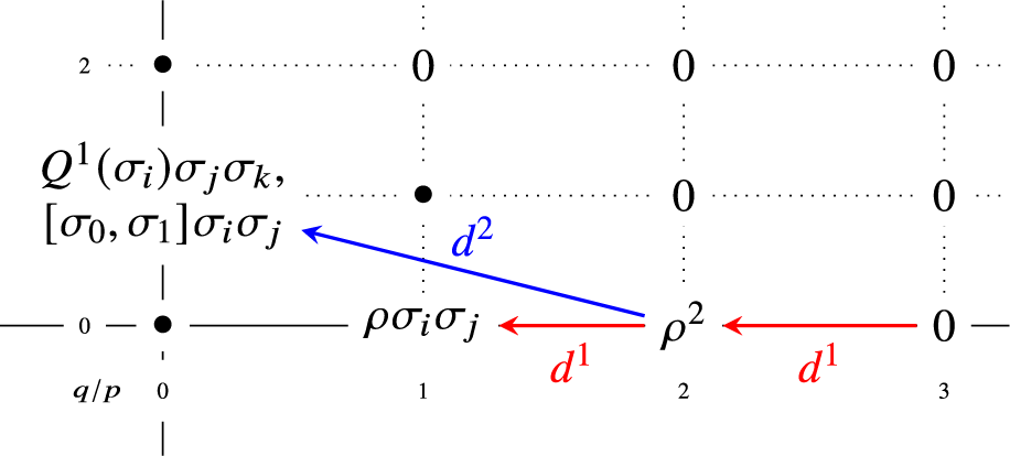


 Open access