


1 Introduction
The study of Borel graphs and Borel equivalence relations has figured prominently in descriptive set theory over the past several decades (see, e.g., [Reference Kechris, Solecki and Todorčević30, Reference Kechris and Miller29, Reference Jackson25, Reference Máthé35, Reference Kechris and Marks28, Reference Pikhurko38, Reference Bernshteyn2, Reference Grebík and Vidnyánszky20, Reference Kechris27]). One of the central themes in this area is the notion of Borel hyperfiniteness. A Borel graph $\mathcal {G}$
is Borel hyperfinite if it can be written as a countable increasing union of Borel graphs with finite connected components, that is,
$\mathcal {G}$
is Borel hyperfinite if it can be written as a countable increasing union of Borel graphs with finite connected components, that is, $\mathcal {G} = \bigcup _{n \in {\mathbb {N}}} \mathcal {G}_n$
, where for each
$\mathcal {G} = \bigcup _{n \in {\mathbb {N}}} \mathcal {G}_n$
, where for each $n \in {\mathbb {N}}$
,
$n \in {\mathbb {N}}$
, $\mathcal {G}_n$
is a Borel graph with finite connected components and
$\mathcal {G}_n$
is a Borel graph with finite connected components and $\mathcal {G}_n\subseteq \mathcal {G}_{n+1}$
.
$\mathcal {G}_n\subseteq \mathcal {G}_{n+1}$
.
Hyperfinite structures arise in various areas of mathematics and theoretical computer science as nontrivial structures of minimal complexity (see, e.g., [Reference Connes11, Reference Connes, Feldman and Weiss12, Reference Harrington, Kechris and Louveau22, Reference Kechris and Miller29, Reference Matui33, Reference Lovász31, Reference Elek16]). In particular, in the theory of countable Borel equivalence relations, the class of Borel hyperfinite equivalence relations is the minimum nontrivial element in the Borel reducibility hierarchy by the Glimm–Effros dichotomy [Reference Glimm19, Reference Effros14, Reference Effros, McAuley and Rao15, Reference Harrington, Kechris and Louveau22]. However, many basic problems about Borel hyperfiniteness remain open (see [Reference Kechris27] for a recent survey). Among these problems, one of the deepest centers around the complexity of hyperfiniteness: While it is immediate from the definition that hyperfiniteness is a $\boldsymbol {\Sigma }^1_2$
notion, it is unknown whether the set of codes of Borel hyperfinite graphs is
$\boldsymbol {\Sigma }^1_2$
notion, it is unknown whether the set of codes of Borel hyperfinite graphs is $\boldsymbol {\Sigma }^1_2$
-complete, that is, maximally complex [Reference Dougherty, Jackson and Kechris13] (see Section 2 for the formal definitions of the complexity notions). The
$\boldsymbol {\Sigma }^1_2$
-complete, that is, maximally complex [Reference Dougherty, Jackson and Kechris13] (see Section 2 for the formal definitions of the complexity notions). The $\boldsymbol {\Sigma }^1_2$
-completeness of Borel hyperfiniteness would rule out a number of conjectured dichotomy theorems [Reference Kechris27].
$\boldsymbol {\Sigma }^1_2$
-completeness of Borel hyperfiniteness would rule out a number of conjectured dichotomy theorems [Reference Kechris27].
In [Reference Conley, Jackson, Marks, Seward and Tucker-Drob10], the authors introduce the notion of Borel asymptotic dimension as an extension of Gromov’s classical notion of asymptotic dimension for metric spaces [Reference Gromov, Niblo and Roller21] to the definable context; they also show that if a locally finite Borel graph has finite Borel asymptotic dimension, then it is Borel hyperfinite [Reference Conley, Jackson, Marks, Seward and Tucker-Drob10, Theorem 7.1]. Despite its recency, Borel asymptotic dimension has become an invaluable tool in the study of Borel hyperfiniteness (see, e.g., [Reference Bernshteyn and Yu4, Reference Naryshkin and Vaccaro36, Reference Iyer and Shinko24]).
While determining the exact complexity of Borel hyperfiniteness remains a major open problem, our main result shows that the notion of finite Borel asymptotic dimension is $\boldsymbol {\Sigma }^1_2$
-complete.
$\boldsymbol {\Sigma }^1_2$
-complete.
Theorem 1.1. The set of locally finite Borel graphs having finite Borel asymptotic dimension is $\boldsymbol {\Sigma }^1_2$
-complete.
$\boldsymbol {\Sigma }^1_2$
-complete.
Theorem 1.1 builds on the celebrated paper of Todorčević and Vidnyánszky [Reference Todorčević and Vidnyánszky41], who showed that locally finite Borel graphs having finite Borel chromatic number form a $\boldsymbol {\Sigma }^1_2$
-complete set, and adds to the growing body of complexity results in Borel combinatorics (see, e.g., [Reference Brandt, Chang, Grebík, Grunau, Rozhoň and Vidnyánszky6, Reference Thornton40, Reference Frisch, Shinko and Vidnyánszky18]).
$\boldsymbol {\Sigma }^1_2$
-complete set, and adds to the growing body of complexity results in Borel combinatorics (see, e.g., [Reference Brandt, Chang, Grebík, Grunau, Rozhoň and Vidnyánszky6, Reference Thornton40, Reference Frisch, Shinko and Vidnyánszky18]).
The main tool we use to prove Theorem 1.1 involves transforming the geometric question of whether a graph generated by a single Borel function has finite Borel asymptotic dimension (see Section 5 for the definition) into a purely combinatorial question concerning the existence of certain forward-recurrent sets. A Borel function f on a standard Borel space X is acyclic if $f^k(x) \neq x$
for every
$f^k(x) \neq x$
for every $x \in X$
and
$x \in X$
and $k \in {\mathbb {N}}^+ = {\mathbb {N}} \setminus \{0 \}$
. We write
$k \in {\mathbb {N}}^+ = {\mathbb {N}} \setminus \{0 \}$
. We write $\mathcal {G}_f$
for the Borel graph generated by f, that is, the graph on X where vertices
$\mathcal {G}_f$
for the Borel graph generated by f, that is, the graph on X where vertices $x, y \in X$
are adjacent if and only if
$x, y \in X$
are adjacent if and only if $x \neq y$
and either
$x \neq y$
and either $f(x) = y$
or
$f(x) = y$
or $f(y) = x$
. A set
$f(y) = x$
. A set $H \subseteq X$
is hitting for f if, for each
$H \subseteq X$
is hitting for f if, for each $x \in X$
, there is
$x \in X$
, there is $k \in {\mathbb {N}}^+$
such that
$k \in {\mathbb {N}}^+$
such that $f^k(x) \in H$
. Given
$f^k(x) \in H$
. Given $r \in {\mathbb {N}}^+$
, the set H is r-forward-independent for f if
$r \in {\mathbb {N}}^+$
, the set H is r-forward-independent for f if $f^k(x) \in H$
implies that
$f^k(x) \in H$
implies that $k> r$
for any
$k> r$
for any $x \in H$
and
$x \in H$
and $k \in {\mathbb {N}}^+$
.
$k \in {\mathbb {N}}^+$
.
Theorem 1.2. Let X be a standard Borel space, and let $f : X \rightarrow X$
be an acyclic Borel function. Then the following are equivalent:
$f : X \rightarrow X$
be an acyclic Borel function. Then the following are equivalent:
-
(i) $\text {asdim}_B(\mathcal {G}_f)$
is finite.
$\text {asdim}_B(\mathcal {G}_f)$
is finite. -
(ii)
$\text {asdim}_B(\mathcal {G}_f)= 1$
. -
(iii) For each
$r \in {\mathbb {N}}^+$
, there is a Borel r-forward-independent hitting set for f.


Remark 1.3. Condition (iii) in Theorem 1.2 is satisfied if, for instance, f is bounded-to-one. This follows from [Reference Kechris, Solecki and Todorčević30, Corollary 5.3]. Furthermore, (iii) is also satisfied when the connectedness relation of $\mathcal {G}_f$
admits a Borel transversal.
$\mathcal {G}_f$
admits a Borel transversal.
Borel graphs with finite Borel asymptotic dimension enjoy certain definable combinatorial properties that are not shared by Borel hyperfinite graphs in general. For instance, Brooks’s theorem, a fundamental result in the theory of graph colorings, fails for Borel colorings [Reference Marks32], even when the graph under consideration is Borel hyperfinite [Reference Conley, Jackson, Marks, Seward and Tucker-Drob9]. However, a version of Brooks’s theorem for Borel colorings, and in fact Borel versions of many local coloring problems that in general only admit solutions up to null sets, can be recovered for Borel graphs with finite Borel asymptotic dimension [Reference Bernshteyn and Weilacher3].
As an application of the techniques used to prove Theorems 1.1 and 1.2, we derive a new complexity result for a homomorphism problem for the class of Borel directed graphs (digraphs for short) generated by a single Borel function. Given a finite digraph H, we follow Thornton [Reference Thornton40] and write $\operatorname {CSP}_B(H)$
for the set (of codes) of Borel digraphs that admit a Borel homomorphism to H, and we also define
$\operatorname {CSP}_B(H)$
for the set (of codes) of Borel digraphs that admit a Borel homomorphism to H, and we also define $\operatorname {CSP}^{\operatorname {function}}_B(H)$
to be the set (of codes) of Borel digraphs generated by a single Borel function that admit a Borel homomorphism to H. Note that when investigating
$\operatorname {CSP}^{\operatorname {function}}_B(H)$
to be the set (of codes) of Borel digraphs generated by a single Borel function that admit a Borel homomorphism to H. Note that when investigating $\operatorname {CSP}^{\operatorname {function}}_B(H)$
, we can without loss of generality assume that H is sinkless, that is, that every vertex of H has at least one outgoing edge.
$\operatorname {CSP}^{\operatorname {function}}_B(H)$
, we can without loss of generality assume that H is sinkless, that is, that every vertex of H has at least one outgoing edge.
Recall that a finite digraph H is ergodic if there are $v\in V(H)$
and
$v\in V(H)$
and $k_0\in \mathbb {N}$
such that, for every
$k_0\in \mathbb {N}$
such that, for every $k\ge k_0$
, there is a directed path of length k that starts and ends at v.Footnote 1 A loop is a directed edge of the form
$k\ge k_0$
, there is a directed path of length k that starts and ends at v.Footnote 1 A loop is a directed edge of the form $(v, v)$
for some
$(v, v)$
for some $v \in V(H)$
. Note that any digraph containing a loop is ergodic.
$v \in V(H)$
. Note that any digraph containing a loop is ergodic.
Theorem 1.4. Let H be a finite sinkless digraph.
-
(i) The digraph H contains a loop if and only if
$\operatorname {CSP}^{\operatorname {function}}_B(H)$
contains all digraphs generated by a single Borel function. In particular, the set
$\operatorname {CSP}^{\operatorname {function}}_B(H)$
is
$\boldsymbol {\Pi }^1_1$
. -
(ii) If H is ergodic and has no loops, then
$\operatorname {CSP}^{\operatorname {function}}_B(H)$
is
$\boldsymbol {\Sigma }^1_2$
-complete. -
(iii) If H is not ergodic, then
$\operatorname {CSP}^{\operatorname {function}}_B(H)$
is
$\boldsymbol {\Pi }^1_1$
.


Remark 1.5 (Connections to CSPs)
Theorem 1.4 is motivated by the classical theory of constraint satisfaction problems (CSPs); see, for example, [Reference Brady5] for a comprehensive overview of the subject. A (fixed-template) constraint satisfaction problem takes the following form: Given a finite structure H, how complicated is it to decide whether a finite structure in the same signature admits a homomorphism to H? The target structure H is called the template, and the set of finite structures admitting a homomorphism to H is denoted $\operatorname {CSP}(H)$
. The well-known CSP dichotomy conjecture, now a theorem, states that every CSP is either solvable in polynomial time or NP-complete.
$\operatorname {CSP}(H)$
. The well-known CSP dichotomy conjecture, now a theorem, states that every CSP is either solvable in polynomial time or NP-complete.
In their foundational paper, Feder and Vardi [Reference Feder and Vardi17] showed that every CSP is polynomial-time equivalent to a digraph CSP, that is, a CSP whose template is a digraph; therefore, resolving the full conjecture amounts to resolving it just for digraph CSPs. A special case of the CSP dichotomy in the case when the template is a sinkless and sourceless digraph was established by Barto, Kozik, and Niven [Reference Barto, Kozik and Niven1]. Later, the full CSP dichotomy conjecture was confirmed independently by Bulatov [Reference Bulatov8] and by Zhuk [Reference Zhuk42, Reference Zhuk43].
Recently, Thornton [Reference Thornton40] initiated the study of the complexity of CSPs in measurable combinatorics. More precisely, given a finite digraph H, we may consider, as above, the set $\operatorname {CSP}_B(H)$
(of codes) of Borel digraphs that admit a Borel homomorphism to H. Among other results, Thornton [Reference Thornton40] proved a Borel analogue of the CSP dichotomy for sinkless and sourceless digraphs; in particular, when H is sinkless and sourceless,
$\operatorname {CSP}_B(H)$
(of codes) of Borel digraphs that admit a Borel homomorphism to H. Among other results, Thornton [Reference Thornton40] proved a Borel analogue of the CSP dichotomy for sinkless and sourceless digraphs; in particular, when H is sinkless and sourceless, $\operatorname {CSP}_B(H)$
is either
$\operatorname {CSP}_B(H)$
is either $\boldsymbol {\Pi }^1_1$
or
$\boldsymbol {\Pi }^1_1$
or $\boldsymbol {\Sigma }^1_2$
-complete. Moreover, these two cases correspond exactly to the classical ones:
$\boldsymbol {\Sigma }^1_2$
-complete. Moreover, these two cases correspond exactly to the classical ones: $\operatorname {CSP}_B(H)$
is
$\operatorname {CSP}_B(H)$
is $\boldsymbol {\Pi }^1_1$
when
$\boldsymbol {\Pi }^1_1$
when $\operatorname {CSP}(H)$
is solvable in polynomial time, and
$\operatorname {CSP}(H)$
is solvable in polynomial time, and $\operatorname {CSP}_B(H)$
is
$\operatorname {CSP}_B(H)$
is $\boldsymbol {\Sigma }^1_2$
-complete when
$\boldsymbol {\Sigma }^1_2$
-complete when $\operatorname {CSP}(H)$
is NP-complete.
$\operatorname {CSP}(H)$
is NP-complete.
Remark 1.6 (
$\operatorname {CSP}_B(H)$
vs
$\operatorname {CSP}^{\operatorname {function}}_B(H)$
)


Note that, when working with $\operatorname {CSP}^{\operatorname {function}}_B(H)$
, we do not impose restrictions on the templates themselves; instead, we consider a subclass of digraphs on which the existence of Borel homomorphisms into H is queried. For any digraph H, since
$\operatorname {CSP}^{\operatorname {function}}_B(H)$
, we do not impose restrictions on the templates themselves; instead, we consider a subclass of digraphs on which the existence of Borel homomorphisms into H is queried. For any digraph H, since $\boldsymbol {\Sigma }^1_2$
is an upper bound for the complexity of
$\boldsymbol {\Sigma }^1_2$
is an upper bound for the complexity of $\operatorname {CSP}_B(H)$
, if
$\operatorname {CSP}_B(H)$
, if $\operatorname {CSP}^{\operatorname {function}}_B(H)$
is
$\operatorname {CSP}^{\operatorname {function}}_B(H)$
is $\boldsymbol {\Sigma }^1_2$
-complete, then
$\boldsymbol {\Sigma }^1_2$
-complete, then $\operatorname {CSP}_B(H)$
is
$\operatorname {CSP}_B(H)$
is $\boldsymbol {\Sigma }^1_2$
-complete as well. The converse does not hold in general (see Figure 1 and its description for a counterexample). However, it is possible that a weaker form of the converse holds; see the next paragraph and Section 6.
$\boldsymbol {\Sigma }^1_2$
-complete as well. The converse does not hold in general (see Figure 1 and its description for a counterexample). However, it is possible that a weaker form of the converse holds; see the next paragraph and Section 6.
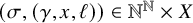
(a) A directed graph H such that $\operatorname {CSP}^{\operatorname {function}}_B(H)$
is
$\operatorname {CSP}^{\operatorname {function}}_B(H)$
is $\boldsymbol {\Pi }^1_1$
. (b) An abstract walk p. (c) The directed graph
$\boldsymbol {\Pi }^1_1$
. (b) An abstract walk p. (c) The directed graph $H^p$
, which has the property that
$H^p$
, which has the property that $\operatorname {CSP}^{\operatorname {function}}_B(H^p)$
is
$\operatorname {CSP}^{\operatorname {function}}_B(H^p)$
is $\boldsymbol {\Sigma }^1_2$
-complete, showing that
$\boldsymbol {\Sigma }^1_2$
-complete, showing that $\operatorname {CSP}_B(H)$
is
$\operatorname {CSP}_B(H)$
is $\boldsymbol {\Sigma }^1_2$
-complete as well.
$\boldsymbol {\Sigma }^1_2$
-complete as well.

Suppose now that H is both sinkless and sourceless. Let p be an abstract walk, that is, a finite sequence of arrows as in Figure 1(b). Define $H^p$
to be the p-power of H, that is, the directed graph on
$H^p$
to be the p-power of H, that is, the directed graph on $V(H)$
where there is a directed edge from x to y if there is a realization in H of the walk p from x to y (see Figure 1(c) for an example). Since H is sinkless and sourceless, it can be easily seen that
$V(H)$
where there is a directed edge from x to y if there is a realization in H of the walk p from x to y (see Figure 1(c) for an example). Since H is sinkless and sourceless, it can be easily seen that $H^p$
is also sinkless and sourceless. If
$H^p$
is also sinkless and sourceless. If $\operatorname {CSP}^{\operatorname {function}}_B(H^p)$
is
$\operatorname {CSP}^{\operatorname {function}}_B(H^p)$
is $\boldsymbol {\Sigma }^1_2$
-complete for some walk p, then so is
$\boldsymbol {\Sigma }^1_2$
-complete for some walk p, then so is $\operatorname {CSP}_B(H)$
; this follows from the fact that, for any function f, the directed graph
$\operatorname {CSP}_B(H)$
; this follows from the fact that, for any function f, the directed graph $\overrightarrow {\mathcal {G}}_f$
generated by f admits a (Borel) homomorphism to
$\overrightarrow {\mathcal {G}}_f$
generated by f admits a (Borel) homomorphism to $H^p$
if and only if the directed graph formed from
$H^p$
if and only if the directed graph formed from $\overrightarrow {\mathcal {G}}_f$
by replacing each directed edge with the path p admits a (Borel) homomorphism to H (we note that this construction is definable in the codes). We leave as an open problem whether the converse holds; see Section 6.
$\overrightarrow {\mathcal {G}}_f$
by replacing each directed edge with the path p admits a (Borel) homomorphism to H (we note that this construction is definable in the codes). We leave as an open problem whether the converse holds; see Section 6.
Remark 1.7 (Connections to the LOCAL model)
Theorem 1.4 provides a connection with the LOCAL model of distributed computing and also serves as a specific instance of an interesting general phenomenon: For “flexible” problems such as $3$
-coloring, there is a nontrivial class of graphs for which it is easy to produce solutions in a distributed way, but it is difficult to determine, for general graphs, whether a solution exists; while for “rigid” problems such as
$3$
-coloring, there is a nontrivial class of graphs for which it is easy to produce solutions in a distributed way, but it is difficult to determine, for general graphs, whether a solution exists; while for “rigid” problems such as $2$
-coloring, it is impossible to construct solutions on any nontrivial class of graphs, but it is easy to check, for general graphs, whether a solution exists.
$2$
-coloring, it is impossible to construct solutions on any nontrivial class of graphs, but it is easy to check, for general graphs, whether a solution exists.
To be precise, recall first that any locally checkable labeling (LCL) problem on oriented paths can be thought of as a digraph homomorphism problem $\Pi _H$
to a finite sinkless digraph H [Reference Brandt, Hirvonen, Korhonen, Lempiäinen, Östergård, Purcell, Rybicki, Suomela and Uznański7]. The classification of LCL problems on oriented paths in the LOCAL model [Reference Brandt, Hirvonen, Korhonen, Lempiäinen, Östergård, Purcell, Rybicki, Suomela and Uznański7] states that:
$\Pi _H$
to a finite sinkless digraph H [Reference Brandt, Hirvonen, Korhonen, Lempiäinen, Östergård, Purcell, Rybicki, Suomela and Uznański7]. The classification of LCL problems on oriented paths in the LOCAL model [Reference Brandt, Hirvonen, Korhonen, Lempiäinen, Östergård, Purcell, Rybicki, Suomela and Uznański7] states that:
-
(i) If H contains a loop, then
$\Pi _H$
can be solved in
$0$
rounds of communication in the LOCAL model. -
(ii) If H is ergodic and has no loops, then
$\Pi _H$
requires
$\Theta (\log ^*(n))$
rounds of communication in the LOCAL model. -
(iii) If H is not ergodic, then
$\Pi _H$
requires
$\Theta (n)$
rounds of communication in the LOCAL model.


Comparing with Theorem 1.4, we see that the existence of an efficient nontrivial LOCAL algorithm for solving $\Pi _H$
on oriented paths is equivalent to
$\Pi _H$
on oriented paths is equivalent to $\operatorname {CSP}^{\operatorname {function}}_B(H)$
being a
$\operatorname {CSP}^{\operatorname {function}}_B(H)$
being a $\boldsymbol {\Sigma }^1_2$
-complete set. If no efficient LOCAL algorithm exists, then
$\boldsymbol {\Sigma }^1_2$
-complete set. If no efficient LOCAL algorithm exists, then $\operatorname {CSP}^{\operatorname {function}}_B(H)$
is
$\operatorname {CSP}^{\operatorname {function}}_B(H)$
is $\boldsymbol {\Pi }^1_1$
.
$\boldsymbol {\Pi }^1_1$
.
The paper is organized as follows. In Section 2, we provide some preliminaries. In Section 3, we prove the main complexity result that we use throughout the rest of the paper. The proof of Theorem 1.4 is given in Section 4. In Section 5, we prove Theorems 1.1 and 1.2. We conclude with some open questions in Section 6.
2 Preliminaries
Let X be a standard Borel space. Given a Borel function $f:X\to X$
, we write
$f:X\to X$
, we write $\mathcal {G}_f$
for the Borel graph generated by f and
$\mathcal {G}_f$
for the Borel graph generated by f and ![]() for the Borel directed graph (digraph) generated by f.
for the Borel directed graph (digraph) generated by f.
Recall that $[{\mathbb {N}}]^{{\mathbb {N}}}$
denotes the space of infinite subsets of
$[{\mathbb {N}}]^{{\mathbb {N}}}$
denotes the space of infinite subsets of ${\mathbb {N}}$
. Each point
${\mathbb {N}}$
. Each point $x \in [{\mathbb {N}}]^{{\mathbb {N}}}$
may be identified with its increasing enumeration
$x \in [{\mathbb {N}}]^{{\mathbb {N}}}$
may be identified with its increasing enumeration $x = (x(n))_{n \in {\mathbb {N}}}$
. The shift function
$x = (x(n))_{n \in {\mathbb {N}}}$
. The shift function $S:[{\mathbb {N}}]^{\mathbb {N}}\to [{\mathbb {N}}]^{\mathbb {N}}$
is defined by
$S:[{\mathbb {N}}]^{\mathbb {N}}\to [{\mathbb {N}}]^{\mathbb {N}}$
is defined by
 $$ \begin{align*}S(x)(n)=x(n+1) \text{ for every } n\in {\mathbb{N}},\end{align*} $$
and the shift graph $\mathcal {G}_S$
is the (undirected) graph on
$\mathcal {G}_S$
is the (undirected) graph on $[{\mathbb {N}}]^{{\mathbb {N}}}$
generated by S.
$[{\mathbb {N}}]^{{\mathbb {N}}}$
generated by S.
For every $x,y\in [{\mathbb {N}}]^{\mathbb {N}}$
, we write
$x,y\in [{\mathbb {N}}]^{\mathbb {N}}$
, we write $y\le ^\infty x$
if the set
$y\le ^\infty x$
if the set $\{n\in {\mathbb {N}}:y(n)\le x(n)\}$
is infinite. We define
$\{n\in {\mathbb {N}}:y(n)\le x(n)\}$
is infinite. We define
 $$ \begin{align*}\text{Dom}=\{(x,y)\in [{\mathbb{N}}]^{\mathbb{N}}\times [{\mathbb{N}}]^{\mathbb{N}}:y\le^\infty x\}.\end{align*} $$
Given sets $X, Y$
and a set
$X, Y$
and a set $B\subseteq X\times Y$
, we write
$B\subseteq X\times Y$
, we write $B_x=\{y\in Y:(x,y)\in B\}$
for each
$B_x=\{y\in Y:(x,y)\in B\}$
for each $x \in X$
.
$x \in X$
.
Let R be a Borel relation on X, let S be a Borel relation on a standard Borel space Y, and assume that R and S have the same arity $d \in {\mathbb {N}}$
. A Borel map
$d \in {\mathbb {N}}$
. A Borel map $\varphi :X\to Y$
is a homomorphism from (X,R) to (Y,S), or from R to S for short, if
$\varphi :X\to Y$
is a homomorphism from (X,R) to (Y,S), or from R to S for short, if
 $$ \begin{align*}(x_0,\dots,x_{d-1})\in R \ \Rightarrow \ (f(x_0),\dots,f(x_{d-1}))\in S\end{align*} $$
for every $(x_i)_{i=0}^{d-1}\in X^d$
.
$(x_i)_{i=0}^{d-1}\in X^d$
.
A finite digraph $H=(V(H),E(H))$
is sinkless if every vertex has an outgoing edge and sourceless if every vertex has an ingoing edge. A directed path in H is a sequence of vertices
$H=(V(H),E(H))$
is sinkless if every vertex has an outgoing edge and sourceless if every vertex has an ingoing edge. A directed path in H is a sequence of vertices $(v_0,\dots , v_k)\subseteq V(H)$
such that
$(v_0,\dots , v_k)\subseteq V(H)$
such that $(v_i,v_{i+1})\in E(H)$
for every
$(v_i,v_{i+1})\in E(H)$
for every $0\le i\le k-1$
. A strong connectivity component of H is an inclusion-maximal set
$0\le i\le k-1$
. A strong connectivity component of H is an inclusion-maximal set $A\subseteq V(H)$
such that, for any vertices
$A\subseteq V(H)$
such that, for any vertices $v, w \in A$
, there is a directed path from v to w in
$v, w \in A$
, there is a directed path from v to w in $H \restriction A$
. We say that H is strongly connected if
$H \restriction A$
. We say that H is strongly connected if $V(H)$
is a strong connectivity component. Note that every finite sinkless digraph contains at least one strong connectivity component since it contains some vertex v for which there is a directed path from v to itself.
$V(H)$
is a strong connectivity component. Note that every finite sinkless digraph contains at least one strong connectivity component since it contains some vertex v for which there is a directed path from v to itself. $\boldsymbol {\Sigma }^1_2$
-completeness. The projective hierarchy provides a general framework for the study of complexity problems in measurable combinatorics. Recall that, given a Polish space X, a set
$\boldsymbol {\Sigma }^1_2$
-completeness. The projective hierarchy provides a general framework for the study of complexity problems in measurable combinatorics. Recall that, given a Polish space X, a set $A \subseteq X$
is
$A \subseteq X$
is $\boldsymbol {\Sigma }^1_2$
if it is the projection of a
$\boldsymbol {\Sigma }^1_2$
if it is the projection of a $\boldsymbol {\Pi }^1_1$
(coanalytic) set (see [Reference Kechris26, Chapter V]). For example, it is easy to see that the set of (codes of) locally finite Borel graphs having finite Borel chromatic number is
$\boldsymbol {\Pi }^1_1$
(coanalytic) set (see [Reference Kechris26, Chapter V]). For example, it is easy to see that the set of (codes of) locally finite Borel graphs having finite Borel chromatic number is $\boldsymbol {\Sigma }^1_2$
. More generally, given any local graph coloring problem, the set of (codes of) locally finite Borel graphs admitting a solution to the problem is
$\boldsymbol {\Sigma }^1_2$
. More generally, given any local graph coloring problem, the set of (codes of) locally finite Borel graphs admitting a solution to the problem is $\boldsymbol {\Sigma }^1_2$
. We refer the reader to [Reference Moschovakis34] and [Reference Frisch, Shinko and Vidnyánszky18, Section 1] for an overview of the coding method.
$\boldsymbol {\Sigma }^1_2$
. We refer the reader to [Reference Moschovakis34] and [Reference Frisch, Shinko and Vidnyánszky18, Section 1] for an overview of the coding method.
Definition 2.1 (
$\boldsymbol {\Sigma }^1_2$
-completeness)

Let A be a subset of a Polish space X. We say that A is $\boldsymbol {\Sigma }^1_2$
-hard if for every Polish space Y and every
$\boldsymbol {\Sigma }^1_2$
-hard if for every Polish space Y and every $\boldsymbol {\Sigma }^1_2$
set
$\boldsymbol {\Sigma }^1_2$
set $B\subseteq Y$
, there is a Borel map
$B\subseteq Y$
, there is a Borel map $f:Y\to X$
such that
$f:Y\to X$
such that $f^{-1}(A) = B$
, that is,
$f^{-1}(A) = B$
, that is, $f(y)\in A$
if and only if
$f(y)\in A$
if and only if $y\in B$
. A set
$y\in B$
. A set $A\subseteq X$
is called
$A\subseteq X$
is called $\boldsymbol {\Sigma }^1_2$
-complete if it is simultaneously
$\boldsymbol {\Sigma }^1_2$
-complete if it is simultaneously $\boldsymbol {\Sigma }^1_2$
-hard and
$\boldsymbol {\Sigma }^1_2$
-hard and $\boldsymbol {\Sigma }^1_2$
.
$\boldsymbol {\Sigma }^1_2$
.
As mentioned in the introduction, Todorčević and Vidnyánszky [Reference Todorčević and Vidnyánszky41] showed that the set of codes of locally finite Borel graphs that have finite Borel chromatic number is a $\boldsymbol {\Sigma }^1_2$
-complete set. In our arguments, we use a general result for proving
$\boldsymbol {\Sigma }^1_2$
-complete set. In our arguments, we use a general result for proving $\boldsymbol {\Sigma }^1_2$
-completeness that builds on [Reference Todorčević and Vidnyánszky41] and was derived recently by Frisch, Shinko, and Vidnyánszky [Reference Frisch, Shinko and Vidnyánszky18, Theorem 3.1]. We refer the reader to [Reference Frisch, Shinko and Vidnyánszky18, Section 1] for the definition of Borel L-structure.
$\boldsymbol {\Sigma }^1_2$
-completeness that builds on [Reference Todorčević and Vidnyánszky41] and was derived recently by Frisch, Shinko, and Vidnyánszky [Reference Frisch, Shinko and Vidnyánszky18, Theorem 3.1]. We refer the reader to [Reference Frisch, Shinko and Vidnyánszky18, Section 1] for the definition of Borel L-structure.
Theorem 2.2 (Theorem 3.1, [Reference Frisch, Shinko and Vidnyánszky18])
Let $\mathcal {H}$
be a Borel L-structure on some Polish space Z, and assume that there exist a Borel L-structure
$\mathcal {H}$
be a Borel L-structure on some Polish space Z, and assume that there exist a Borel L-structure $\mathcal {G}$
on
$\mathcal {G}$
on $[\mathbb {N}]^{\mathbb {N}}$
that does not admit a Borel homomorphism to
$[\mathbb {N}]^{\mathbb {N}}$
that does not admit a Borel homomorphism to $\mathcal {H}$
and a Borel map
$\mathcal {H}$
and a Borel map $\Phi : \text {Dom}\to Z$
so that, for each x, we have that
$\Phi : \text {Dom}\to Z$
so that, for each x, we have that $\Phi _x$
is a homomorphism from
$\Phi _x$
is a homomorphism from $\mathcal {G}\upharpoonright \text {Dom}_x$
to
$\mathcal {G}\upharpoonright \text {Dom}_x$
to $\mathcal {H}$
. Then the Borel L-structures that admit a Borel homomorphism to
$\mathcal {H}$
. Then the Borel L-structures that admit a Borel homomorphism to $\mathcal {H}$
form a
$\mathcal {H}$
form a $\boldsymbol {\Sigma }^1_2$
-complete set.
$\boldsymbol {\Sigma }^1_2$
-complete set.
In fact, we use a slight strengthening of Theorem 2.2 that follows from the proof of [Reference Frisch, Shinko and Vidnyánszky18, Theorem 3.1]. Given an L-structure $\mathcal {G}$
on
$\mathcal {G}$
on $[\mathbb {N}]^{\mathbb {N}}$
, write
$[\mathbb {N}]^{\mathbb {N}}$
, write $\mathcal {G}'$
for the L-structure on
$\mathcal {G}'$
for the L-structure on ${\mathbb {N}}^{\mathbb {N}}\times [\mathbb {N}]^{\mathbb {N}}$
where each vertical section is a copy of
${\mathbb {N}}^{\mathbb {N}}\times [\mathbb {N}]^{\mathbb {N}}$
where each vertical section is a copy of $\mathcal {G}$
and no additional elements are related.
$\mathcal {G}$
and no additional elements are related.
Theorem 2.3. Let $\mathcal {H}$
be as in Theorem 2.2. Then there is a Borel set
$\mathcal {H}$
be as in Theorem 2.2. Then there is a Borel set $B\subseteq \mathbb {N}^{\mathbb {N}}\times \mathbb {N}^{\mathbb {N}}\times [\mathbb {N}]^{\mathbb {N}}$
such that the set
$B\subseteq \mathbb {N}^{\mathbb {N}}\times \mathbb {N}^{\mathbb {N}}\times [\mathbb {N}]^{\mathbb {N}}$
such that the set
 $$ \begin{align*} \{\sigma\in {\mathbb{N}}^{\mathbb{N}}: \text{ there is a Borel homomorphism from } (\mathcal{G}' \restriction B_{\sigma}) \text{ to } \mathcal{H} \} \end{align*} $$
is $\boldsymbol {\Sigma }^1_2$
-complete.
$\boldsymbol {\Sigma }^1_2$
-complete.
3 Complexity of forward-independent hitting sets
In this section, we use Theorem 2.3 to deduce the following theorem, which immediately implies that the set (of codes) of Borel functions admitting Borel forward-independent hitting sets is $\boldsymbol {\Sigma }^1_2$
-complete. Our main result, Theorem 1.1, is a corollary of Theorem 3.1 together with Theorem 1.2, which is proved in Section 5.
$\boldsymbol {\Sigma }^1_2$
-complete. Our main result, Theorem 1.1, is a corollary of Theorem 3.1 together with Theorem 1.2, which is proved in Section 5.
Theorem 3.1. There are a standard Borel space X and a finite-to-one acyclic Borel function
 $$ \begin{align*}f:\mathbb{N}^{\mathbb{N}}\times X\to \mathbb{N}^{\mathbb{N}}\times X\end{align*} $$
with the property that, for every $\sigma \in \mathbb {N}^{\mathbb {N}}$
, there exists
$\sigma \in \mathbb {N}^{\mathbb {N}}$
, there exists $f_\sigma : X\to X$
such that
$f_\sigma : X\to X$
such that
 $$ \begin{align*}f(\sigma,x)=(\sigma,f_\sigma(x)) \text{ for every } (\sigma,x)\in \mathbb{N}^{\mathbb{N}}\times X,\end{align*} $$
and
 $$ \begin{align} \{\sigma\in \mathbb{N}^{\mathbb{N}}: \forall r\in \mathbb{N}^+ \ f_\sigma \ \text{ admits a Borel } r \text{-forward-independent hitting set} \} \end{align} $$
is $\boldsymbol {\Sigma }^1_2$
-complete.
$\boldsymbol {\Sigma }^1_2$
-complete.
Additionally, for every $r\in \mathbb {N}^+$
, there is a Borel function f as above such that
$r\in \mathbb {N}^+$
, there is a Borel function f as above such that
 $$ \begin{align} \{\sigma\in \mathbb{N}^{\mathbb{N}}: f_\sigma \ \text{ admits a Borel } r \text{-forward-independent hitting set} \} \end{align} $$
is $\boldsymbol {\Sigma }^1_2$
-complete.
$\boldsymbol {\Sigma }^1_2$
-complete.
For each $r \in {\mathbb {N}}^+$
, let
$r \in {\mathbb {N}}^+$
, let $\mathcal {D}_r$
be the digraph on
$\mathcal {D}_r$
be the digraph on ${\mathbb {N}}$
such that there is a directed edge from k to
${\mathbb {N}}$
such that there is a directed edge from k to $\ell $
if and only if
$\ell $
if and only if $k> 0$
and
$k> 0$
and $\ell = k - 1$
or
$\ell = k - 1$
or $k = 0$
and
$k = 0$
and $\ell \geq r$
(see Figure 2).
$\ell \geq r$
(see Figure 2).
The structure $\mathcal {D}_r$
on
$\mathcal {D}_r$
on ${\mathbb {N}}$
for various values of
${\mathbb {N}}$
for various values of $r \in {\mathbb {N}}^+$
.
$r \in {\mathbb {N}}^+$
.

Lemma 3.4. Let $f:X\to X$
be an acyclic Borel function, and let
$f:X\to X$
be an acyclic Borel function, and let $r\in \mathbb {N}^+$
. Then the following are equivalent:
$r\in \mathbb {N}^+$
. Then the following are equivalent:
-
(i) There is a Borel r-forward-independent hitting set for f.
-
(ii) There is a Borel map
$\varphi :X\to \mathbb {N}$
that is a homomorphism from to
$(\mathbb {N},\mathcal {D}_r)$
.


Proof. (i) $\implies $
(ii). Let
$\implies $
(ii). Let $H \subseteq X$
be a Borel r-forward-independent hitting set for f. Define a Borel map
$H \subseteq X$
be a Borel r-forward-independent hitting set for f. Define a Borel map $\varphi : X \rightarrow {\mathbb {N}}$
by letting
$\varphi : X \rightarrow {\mathbb {N}}$
by letting $\varphi (x)$
be the least
$\varphi (x)$
be the least $k \in {\mathbb {N}}$
such that
$k \in {\mathbb {N}}$
such that $f^k(x) \in H$
. Note that
$f^k(x) \in H$
. Note that $\varphi (x) = 0$
if and only if
$\varphi (x) = 0$
if and only if $x \in H$
. To see that
$x \in H$
. To see that $\varphi $
is a homomorphism, let
$\varphi $
is a homomorphism, let $x\in X$
and observe that there is a directed edge from
$x\in X$
and observe that there is a directed edge from $\varphi (x)$
to
$\varphi (x)$
to $\varphi (f(x))$
; indeed, if
$\varphi (f(x))$
; indeed, if $\varphi (x)> 0$
, then
$\varphi (x)> 0$
, then $\varphi (f(x)) = \varphi (x) - 1$
, and if
$\varphi (f(x)) = \varphi (x) - 1$
, and if $\varphi (x) = 0$
, then
$\varphi (x) = 0$
, then $x \in H$
, which implies that
$x \in H$
, which implies that $\varphi (f(x))\ge r$
since H is r-forward-independent.
$\varphi (f(x))\ge r$
since H is r-forward-independent.
(ii) $\implies $
(i). Let
$\implies $
(i). Let $\varphi : \overrightarrow {\mathcal {G}}_f \rightarrow \mathcal {D}_r$
be a Borel homomorphism. Set
$\varphi : \overrightarrow {\mathcal {G}}_f \rightarrow \mathcal {D}_r$
be a Borel homomorphism. Set $H = \varphi ^{-1}(\{0 \})$
. Then clearly H is Borel. To see that H is r-forward-independent, suppose
$H = \varphi ^{-1}(\{0 \})$
. Then clearly H is Borel. To see that H is r-forward-independent, suppose $x, y \in H$
with
$x, y \in H$
with $f^k(x) = y$
for some
$f^k(x) = y$
for some $k> 0$
. Then
$k> 0$
. Then $\varphi (x) = 0$
, so
$\varphi (x) = 0$
, so $\varphi (f^i(x))> 0$
whenever
$\varphi (f^i(x))> 0$
whenever $1 \leq i \leq r$
. Since
$1 \leq i \leq r$
. Since $\varphi (f^k(x)) = 0$
, we have
$\varphi (f^k(x)) = 0$
, we have $k> r$
. To see that H is hitting for f, let
$k> r$
. To see that H is hitting for f, let $x \in X$
and observe that
$x \in X$
and observe that $f^{\varphi (x)}(x)\in H$
as
$f^{\varphi (x)}(x)\in H$
as $\varphi $
is a homomorphism.
$\varphi $
is a homomorphism.
Now we are ready to prove Theorem 3.1. The proof strategy is as follows: We show first that, while there are no Borel forward-independent hitting sets for S on the entirety of $[{\mathbb {N}}]^{{\mathbb {N}}}$
, such sets can be constructed for S on the nondominating subsets of
$[{\mathbb {N}}]^{{\mathbb {N}}}$
, such sets can be constructed for S on the nondominating subsets of $[{\mathbb {N}}]^{{\mathbb {N}}}$
, that is, the sets of the form
$[{\mathbb {N}}]^{{\mathbb {N}}}$
, that is, the sets of the form $\text {Dom}_x$
where
$\text {Dom}_x$
where $x \in [{\mathbb {N}}]^{{\mathbb {N}}}$
; furthermore, this construction can be done in a uniform Borel way. This then allows us to apply [Reference Frisch, Shinko and Vidnyánszky18, Theorem 3.1], which gives the
$x \in [{\mathbb {N}}]^{{\mathbb {N}}}$
; furthermore, this construction can be done in a uniform Borel way. This then allows us to apply [Reference Frisch, Shinko and Vidnyánszky18, Theorem 3.1], which gives the $\boldsymbol {\Sigma }^1_2$
-completeness of the sets (3.2) and (3.3).
$\boldsymbol {\Sigma }^1_2$
-completeness of the sets (3.2) and (3.3).
Proof of Theorem 3.1
We first fix $r \in {\mathbb {N}}^+$
and prove that there are a standard Borel space X and a Borel function
$r \in {\mathbb {N}}^+$
and prove that there are a standard Borel space X and a Borel function $f:\mathbb {N}^{\mathbb {N}}\times X\to \mathbb {N}^{\mathbb {N}}\times X$
as in the statement of Theorem 3.1 such that the set (3.3) is
$f:\mathbb {N}^{\mathbb {N}}\times X\to \mathbb {N}^{\mathbb {N}}\times X$
as in the statement of Theorem 3.1 such that the set (3.3) is $\boldsymbol {\Sigma }^1_2$
-complete. At the end of the proof, we explain how to reselect X and f so that the set (3.2) is
$\boldsymbol {\Sigma }^1_2$
-complete. At the end of the proof, we explain how to reselect X and f so that the set (3.2) is $\boldsymbol {\Sigma }^1_2$
-complete.
$\boldsymbol {\Sigma }^1_2$
-complete.
Recall that ![]() is the Borel digraph on
is the Borel digraph on $[{\mathbb {N}}]^{{\mathbb {N}}}$
induced by the shift function S on
$[{\mathbb {N}}]^{{\mathbb {N}}}$
induced by the shift function S on $[{\mathbb {N}}]^{{\mathbb {N}}}$
. Note that there is no Borel map
$[{\mathbb {N}}]^{{\mathbb {N}}}$
. Note that there is no Borel map $\varphi :[{\mathbb {N}}]^{\mathbb {N}}\to \mathbb {N}$
that is a homomorphism from
$\varphi :[{\mathbb {N}}]^{\mathbb {N}}\to \mathbb {N}$
that is a homomorphism from ![]() to
to $({\mathbb {N}},\mathcal {D}_r)$
. This follows, for example, from [Reference Kechris, Solecki and Todorčević30, Example 3.2], since the existence of a Borel r-forward-independent hitting set for S would imply that the Borel chromatic number of
$({\mathbb {N}},\mathcal {D}_r)$
. This follows, for example, from [Reference Kechris, Solecki and Todorčević30, Example 3.2], since the existence of a Borel r-forward-independent hitting set for S would imply that the Borel chromatic number of $\mathcal {G}_S$
is finite.
$\mathcal {G}_S$
is finite.
In order to apply Theorem 2.3, we must show that there is a Borel map $\varphi _r : \text {Dom} \to {\mathbb {N}}$
such that, for each
$\varphi _r : \text {Dom} \to {\mathbb {N}}$
such that, for each $x \in [{\mathbb {N}}]^{{\mathbb {N}}}$
, the restriction
$x \in [{\mathbb {N}}]^{{\mathbb {N}}}$
, the restriction $\varphi _r \restriction \text {Dom}_x$
is a homomorphism from
$\varphi _r \restriction \text {Dom}_x$
is a homomorphism from $\overrightarrow {\mathcal {G}}_S \restriction \text {Dom}_x$
to
$\overrightarrow {\mathcal {G}}_S \restriction \text {Dom}_x$
to $\mathcal {D}_r$
, where
$\mathcal {D}_r$
, where ![]() denotes the sub-digraph of
denotes the sub-digraph of ![]() induced by
induced by $\text {Dom}_x$
.
$\text {Dom}_x$
.
Set $x(-r) = 0$
for all
$x(-r) = 0$
for all $x \in [{\mathbb {N}}]^{{\mathbb {N}}}$
. Define
$x \in [{\mathbb {N}}]^{{\mathbb {N}}}$
. Define $\mathcal {H}_r \subseteq ([{\mathbb {N}}]^{{\mathbb {N}}})^2$
by
$\mathcal {H}_r \subseteq ([{\mathbb {N}}]^{{\mathbb {N}}})^2$
by $(x, y) \in \mathcal {H}_r$
if and only if
$(x, y) \in \mathcal {H}_r$
if and only if $\vert [x(2rn - r), x(2rn + r)) \cap y \vert \equiv _{2r} 0$
, where
$\vert [x(2rn - r), x(2rn + r)) \cap y \vert \equiv _{2r} 0$
, where $n \in {\mathbb {N}}$
is minimal such that
$n \in {\mathbb {N}}$
is minimal such that $[x(2rn - r), x(2rn + r)) \cap y \neq \emptyset $
. Observe that
$[x(2rn - r), x(2rn + r)) \cap y \neq \emptyset $
. Observe that $\mathcal {H}_r$
is Borel.
$\mathcal {H}_r$
is Borel.
Claim 3.5. If $(x, y) \in \text {Dom}$
, then there is
$(x, y) \in \text {Dom}$
, then there is $n \in {\mathbb {N}}$
such that
$n \in {\mathbb {N}}$
such that $\vert [x(2rn - r), x(2rn + r)) \cap y \vert \geq 2r$
.
$\vert [x(2rn - r), x(2rn + r)) \cap y \vert \geq 2r$
.
Proof. Let $(x,y)\in \text {Dom}$
and assume for contradiction that there is no
$(x,y)\in \text {Dom}$
and assume for contradiction that there is no $n\in {\mathbb {N}}$
such that
$n\in {\mathbb {N}}$
such that $\vert [x(2rn - r), x(2rn + r)) \cap y \vert \ge 2r$
. For each
$\vert [x(2rn - r), x(2rn + r)) \cap y \vert \ge 2r$
. For each $n \in {\mathbb {N}}$
, let
$n \in {\mathbb {N}}$
, let $\ell _n\in {\mathbb {N}}$
be minimal such that
$\ell _n\in {\mathbb {N}}$
be minimal such that $y(\ell _n)\ge x(2rn-r)$
; it follows from the assumption that
$y(\ell _n)\ge x(2rn-r)$
; it follows from the assumption that $\ell _{n+1}<\ell _n+2r$
. Hence,
$\ell _{n+1}<\ell _n+2r$
. Hence, $\ell _n \leq 2rn - n$
for each
$\ell _n \leq 2rn - n$
for each $n \in {\mathbb {N}}$
. So, there is
$n \in {\mathbb {N}}$
. So, there is $n_0\in {\mathbb {N}}$
such that
$n_0\in {\mathbb {N}}$
such that $\ell _{n}< 2rn-3r$
for every
$\ell _{n}< 2rn-3r$
for every $n\ge n_0$
. Let
$n\ge n_0$
. Let $k\ge \ell _{n_0}$
, and let
$k\ge \ell _{n_0}$
, and let $n\ge n_0$
be minimal such that
$n\ge n_0$
be minimal such that $k\ge \ell _n$
. Then we have
$k\ge \ell _n$
. Then we have
 $$ \begin{align*}y(k)\ge y(\ell_n)\ge x(2rn-r)> x(k)\end{align*} $$
as $2rn-r> \ell _n+2r > \ell _{n+1} \ge k$
, which is a contradiction as
$2rn-r> \ell _n+2r > \ell _{n+1} \ge k$
, which is a contradiction as $y\le ^\infty x$
.
$y\le ^\infty x$
.
Now for each $(x, y) \in \text {Dom}$
, define
$(x, y) \in \text {Dom}$
, define $\varphi _r(x, y)$
to be the least
$\varphi _r(x, y)$
to be the least $k \in {\mathbb {N}}$
such that
$k \in {\mathbb {N}}$
such that $S^k(y) \in (\mathcal {H}_r)_x$
. By Claim 3.5, we have that
$S^k(y) \in (\mathcal {H}_r)_x$
. By Claim 3.5, we have that $\varphi _r$
is well-defined and it is easy to check that it is Borel as
$\varphi _r$
is well-defined and it is easy to check that it is Borel as $\mathcal {H}_r$
is Borel. To see that
$\mathcal {H}_r$
is Borel. To see that $\varphi _r \restriction \text {Dom}_x$
is a homomorphism from
$\varphi _r \restriction \text {Dom}_x$
is a homomorphism from $\overrightarrow {\mathcal {G}}_S \restriction \text {Dom}_x$
to
$\overrightarrow {\mathcal {G}}_S \restriction \text {Dom}_x$
to $\mathcal {D}_r$
for each
$\mathcal {D}_r$
for each $x \in [{\mathbb {N}}]^{{\mathbb {N}}}$
, note that, if
$x \in [{\mathbb {N}}]^{{\mathbb {N}}}$
, note that, if $y, y' \in \text {Dom}_x$
and
$y, y' \in \text {Dom}_x$
and $S(y) = y'$
, then
$S(y) = y'$
, then $\varphi _r(x, y) = 0$
implies
$\varphi _r(x, y) = 0$
implies $\varphi _r(x, S(y)) \geq r$
since
$\varphi _r(x, S(y)) \geq r$
since
 $$ \begin{align*}\vert [x(2rn - r), x(2rn + r)) \cap S(y) \vert \equiv_{2r} 2r-1,\end{align*} $$
where $n \in {\mathbb {N}}$
is minimal such that
$n \in {\mathbb {N}}$
is minimal such that $[x(2rn - r), x(2rn + r)) \cap y \neq \emptyset $
. If
$[x(2rn - r), x(2rn + r)) \cap y \neq \emptyset $
. If $\varphi _r(x, y)> 0$
, then
$\varphi _r(x, y)> 0$
, then $\varphi _r(x, S(y)) = \varphi _r(x, y) - 1$
by the definition.
$\varphi _r(x, S(y)) = \varphi _r(x, y) - 1$
by the definition.
Now we are ready to finish the first part of the proof. Note that the assumptions of Theorem 2.3 are satisfied by the construction of $\varphi _r$
above. Hence, there is a Borel set
$\varphi _r$
above. Hence, there is a Borel set $B\subseteq {\mathbb {N}}^{\mathbb {N}}\times {\mathbb {N}}^{\mathbb {N}}\times [{\mathbb {N}}]^{\mathbb {N}}$
such that
$B\subseteq {\mathbb {N}}^{\mathbb {N}}\times {\mathbb {N}}^{\mathbb {N}}\times [{\mathbb {N}}]^{\mathbb {N}}$
such that
 $$ \begin{align} \{\sigma\in {\mathbb{N}}^{\mathbb{N}}: \text{ there is a Borel homomorphism from } (\overrightarrow{\mathcal{G}}^{\prime}_S \restriction B_{\sigma}) \text{ to } \mathcal{D}_r \} \end{align} $$
is $\boldsymbol {\Sigma }^1_2$
-complete, where
$\boldsymbol {\Sigma }^1_2$
-complete, where $\overrightarrow {\mathcal {G}}^{\prime }_S$
is the digraph on
$\overrightarrow {\mathcal {G}}^{\prime }_S$
is the digraph on ${\mathbb {N}}^{{\mathbb {N}}} \times [{\mathbb {N}}]^{{\mathbb {N}}}$
such that there is a directed edge from
${\mathbb {N}}^{{\mathbb {N}}} \times [{\mathbb {N}}]^{{\mathbb {N}}}$
such that there is a directed edge from $(\gamma , x)$
to
$(\gamma , x)$
to $(\delta , y)$
if and only if
$(\delta , y)$
if and only if $\gamma = \delta $
and
$\gamma = \delta $
and $S(x) = y$
. Let
$S(x) = y$
. Let
 $$ \begin{align*}Y=\{(\sigma,\gamma,x)\in B:(\sigma,\gamma,S(x))\not\in B\}\end{align*} $$
and observe that Y is a Borel set. Set also $Z=({\mathbb {N}}^{\mathbb {N}}\times {\mathbb {N}}^{\mathbb {N}}\times [{\mathbb {N}}]^{\mathbb {N}})\setminus B$
. We define
$Z=({\mathbb {N}}^{\mathbb {N}}\times {\mathbb {N}}^{\mathbb {N}}\times [{\mathbb {N}}]^{\mathbb {N}})\setminus B$
. We define
 $$ \begin{align*}X=\bigsqcup_{\ell\in \mathbb{N}} ({\mathbb{N}}^{\mathbb{N}}\times [{\mathbb{N}}]^{\mathbb{N}}\times \{\ell\})\end{align*} $$
and a function f on $\mathbb {N}^{\mathbb {N}}\times X$
as follows. If
$\mathbb {N}^{\mathbb {N}}\times X$
as follows. If $(\sigma ,(\gamma ,x,\ell ))\in {\mathbb {N}}^{{\mathbb {N}}} \times X$
has the property that
$(\sigma ,(\gamma ,x,\ell ))\in {\mathbb {N}}^{{\mathbb {N}}} \times X$
has the property that $(\sigma ,\gamma ,x)\not \in Y\cup Z$
, then we set
$(\sigma ,\gamma ,x)\not \in Y\cup Z$
, then we set $f(\sigma ,(\gamma ,x,\ell ))=(\sigma ,(\gamma ,S(x),\ell ))$
. Otherwise, we have that
$f(\sigma ,(\gamma ,x,\ell ))=(\sigma ,(\gamma ,S(x),\ell ))$
. Otherwise, we have that $(\sigma ,\gamma ,x)\in Y\cup Z$
and we let
$(\sigma ,\gamma ,x)\in Y\cup Z$
and we let $f(\sigma ,(\gamma ,x,\ell ))=(\sigma ,(\gamma ,x,\ell +1))$
. Then
$f(\sigma ,(\gamma ,x,\ell ))=(\sigma ,(\gamma ,x,\ell +1))$
. Then $f: {\mathbb {N}}^{{\mathbb {N}}} \times X\to {\mathbb {N}}^{{\mathbb {N}}} \times X$
is a finite-to-one acyclic Borel function. Fix
$f: {\mathbb {N}}^{{\mathbb {N}}} \times X\to {\mathbb {N}}^{{\mathbb {N}}} \times X$
is a finite-to-one acyclic Borel function. Fix $\sigma \in {\mathbb {N}}^{{\mathbb {N}}}$
, and let
$\sigma \in {\mathbb {N}}^{{\mathbb {N}}}$
, and let $f_{\sigma }$
be the function on X such that
$f_{\sigma }$
be the function on X such that $f(\sigma , (\gamma , x, \ell )) = (\sigma , f_{\sigma }(\gamma , x, \ell ))$
for all
$f(\sigma , (\gamma , x, \ell )) = (\sigma , f_{\sigma }(\gamma , x, \ell ))$
for all $(\gamma , x, \ell ) \in X$
. Note that the collection
$(\gamma , x, \ell ) \in X$
. Note that the collection $\{f_\sigma \}_{\sigma \in \mathbb {N}^{\mathbb {N}}}$
is well-defined.
$\{f_\sigma \}_{\sigma \in \mathbb {N}^{\mathbb {N}}}$
is well-defined.
To complete this part of the proof, we show that the sets (3.6) and (3.3) coincide. Define a set $T \subseteq X$
by
$T \subseteq X$
by $(\gamma , x, \ell ) \in T$
if
$(\gamma , x, \ell ) \in T$
if $\ell = 0$
and
$\ell = 0$
and $(\sigma , \gamma , x) \in Y \cup Z$
, and let
$(\sigma , \gamma , x) \in Y \cup Z$
, and let $\mathcal {C}$
denote the collection of connected components of the graph
$\mathcal {C}$
denote the collection of connected components of the graph $\mathcal {G}_{f_{\sigma }}$
on X generated by
$\mathcal {G}_{f_{\sigma }}$
on X generated by $f_{\sigma }$
containing a point
$f_{\sigma }$
containing a point $(\gamma , x, \ell ) \in X$
such that
$(\gamma , x, \ell ) \in X$
such that $(\sigma , \gamma , x) \in Y \cup Z$
. Then T is a Borel transversal for the connectedness relation of
$(\sigma , \gamma , x) \in Y \cup Z$
. Then T is a Borel transversal for the connectedness relation of $\mathcal {G}_{f_{\sigma }} \restriction \bigcup \mathcal {C}$
. Therefore, since
$\mathcal {G}_{f_{\sigma }} \restriction \bigcup \mathcal {C}$
. Therefore, since $f_{\sigma }$
is acyclic, we have that
$f_{\sigma }$
is acyclic, we have that $f_{\sigma } \restriction \bigcup \mathcal {C}$
admits a Borel r-forward-independent hitting set by Remark 1.3. It follows that the sets (3.6) and (3.3) coincide, as required.
$f_{\sigma } \restriction \bigcup \mathcal {C}$
admits a Borel r-forward-independent hitting set by Remark 1.3. It follows that the sets (3.6) and (3.3) coincide, as required.
We now explain how to modify the proof to obtain X and f so that (3.2) is $\boldsymbol {\Sigma }^1_2$
-complete: Consider a language consisting of countably many binary relation symbols
$\boldsymbol {\Sigma }^1_2$
-complete: Consider a language consisting of countably many binary relation symbols $(\mathcal {R}_r)_{r \in {\mathbb {N}}^+}$
. For each
$(\mathcal {R}_r)_{r \in {\mathbb {N}}^+}$
. For each $r \in {\mathbb {N}}^+$
, interpret
$r \in {\mathbb {N}}^+$
, interpret $\mathcal {R}_r$
in
$\mathcal {R}_r$
in ${\mathbb {N}}$
as the edge relation of
${\mathbb {N}}$
as the edge relation of $\mathcal {D}_r$
, and apply Theorem 2.3 to obtain a Borel set
$\mathcal {D}_r$
, and apply Theorem 2.3 to obtain a Borel set $B \subseteq {\mathbb {N}}^{{\mathbb {N}}} \times {\mathbb {N}}^{{\mathbb {N}}} \times [{\mathbb {N}}]^{{\mathbb {N}}}$
such that
$B \subseteq {\mathbb {N}}^{{\mathbb {N}}} \times {\mathbb {N}}^{{\mathbb {N}}} \times [{\mathbb {N}}]^{{\mathbb {N}}}$
such that
 $$ \begin{align} \{\sigma\in {\mathbb{N}}^{\mathbb{N}}: \forall r\in {\mathbb{N}}^+ \text{ there is a Borel homomorphism from } (\overrightarrow{\mathcal{G}}^{\prime}_S \restriction B_{\sigma}) \text{ to } \mathcal{D}_r \} \end{align} $$
is $\boldsymbol {\Sigma }^1_2$
-complete. The rest of the proof proceeds in the same way.
$\boldsymbol {\Sigma }^1_2$
-complete. The rest of the proof proceeds in the same way.
Remark 3.8. In personal communication, Alex Kastner pointed out that the Borel set $B \subseteq {\mathbb {N}}^{{\mathbb {N}}} \times {\mathbb {N}}^{{\mathbb {N}}} \times [{\mathbb {N}}]^{{\mathbb {N}}}$
obtained from the application of Theorem 2.3 can be chosen so that, for each
$B \subseteq {\mathbb {N}}^{{\mathbb {N}}} \times {\mathbb {N}}^{{\mathbb {N}}} \times [{\mathbb {N}}]^{{\mathbb {N}}}$
obtained from the application of Theorem 2.3 can be chosen so that, for each $\sigma , \gamma \in {\mathbb {N}}^{{\mathbb {N}}}$
, the section
$\sigma , \gamma \in {\mathbb {N}}^{{\mathbb {N}}}$
, the section $B_{\sigma , \gamma }$
is
$B_{\sigma , \gamma }$
is $\mathcal {G}_S$
-invariant. This allows one to define
$\mathcal {G}_S$
-invariant. This allows one to define $X = {\mathbb {N}}^{{\mathbb {N}}} \times [{\mathbb {N}}]^{{\mathbb {N}}}$
and
$X = {\mathbb {N}}^{{\mathbb {N}}} \times [{\mathbb {N}}]^{{\mathbb {N}}}$
and $f(\sigma , \gamma , x) = (\sigma , \gamma , S(x))$
directly in the proof of Theorem 3.1.
$f(\sigma , \gamma , x) = (\sigma , \gamma , S(x))$
directly in the proof of Theorem 3.1.
4 The classification of
$\operatorname {CSP}^{\operatorname {function}}_B(H)$

This section is devoted to a proof of Theorem 1.4. As in the proof of Theorem 3.1, we utilize [Reference Frisch, Shinko and Vidnyánszky18, Theorem 3.1].
Recall that the set of codes for Borel functions on a fixed standard Borel space X is $\boldsymbol {\Pi }^1_1$
[Reference Héra, Keleti and Máthé23, Lemma A.3]. For the remainder of the section, we fix a finite sinkless digraph H.
$\boldsymbol {\Pi }^1_1$
[Reference Héra, Keleti and Máthé23, Lemma A.3]. For the remainder of the section, we fix a finite sinkless digraph H.
Proof of Theorem 1.4
(i). Let X be standard Borel, and let f be a Borel function on X. If $(v,v)$
is a loop in H, then the function
$(v,v)$
is a loop in H, then the function $\psi : X \to V(H)$
defined by
$\psi : X \to V(H)$
defined by $\psi (x) = v$
for all
$\psi (x) = v$
for all $x \in X$
is clearly a Borel digraph homomorphism.
$x \in X$
is clearly a Borel digraph homomorphism.
Conversely, if $\operatorname {CSP}^{\operatorname {function}}_B(H)$
contains all Borel digraphs, then in particular it contains the shift digraph
$\operatorname {CSP}^{\operatorname {function}}_B(H)$
contains all Borel digraphs, then in particular it contains the shift digraph $\overrightarrow {\mathcal {G}}_S$
. Let
$\overrightarrow {\mathcal {G}}_S$
. Let $\psi :[{\mathbb {N}}]^{\mathbb {N}}\to V(H)$
be a Borel homomorphism from
$\psi :[{\mathbb {N}}]^{\mathbb {N}}\to V(H)$
be a Borel homomorphism from $\overrightarrow {\mathcal {G}}_S$
to H. By the Galvin–Prikry theorem, since
$\overrightarrow {\mathcal {G}}_S$
to H. By the Galvin–Prikry theorem, since $V(H)$
is finite, there are
$V(H)$
is finite, there are $v\in V(H)$
and
$v\in V(H)$
and $y\in [{\mathbb {N}}]^{\mathbb {N}}$
such that
$y\in [{\mathbb {N}}]^{\mathbb {N}}$
such that $\psi (S^k(y))=v$
for every
$\psi (S^k(y))=v$
for every $k\in {\mathbb {N}}$
. Consequently,
$k\in {\mathbb {N}}$
. Consequently, $(v,v)$
is a loop in H, and this completes the proof.
$(v,v)$
is a loop in H, and this completes the proof.
(ii). Assume that H is an ergodic digraph with no loops. Then by the previous paragraph, we have $\overrightarrow {\mathcal {G}}_S\not \in \operatorname {CSP}^{\operatorname {function}}_B(H)$
. The next result, Proposition 4.2, guarantees that [Reference Frisch, Shinko and Vidnyánszky18, Theorem 3.1] can be used as in the proof of Theorem 3.1 to obtain an acyclic Borel function
$\overrightarrow {\mathcal {G}}_S\not \in \operatorname {CSP}^{\operatorname {function}}_B(H)$
. The next result, Proposition 4.2, guarantees that [Reference Frisch, Shinko and Vidnyánszky18, Theorem 3.1] can be used as in the proof of Theorem 3.1 to obtain an acyclic Borel function $f=(f_\sigma )_{\sigma \in {{\mathbb {N}}^{\mathbb {N}}}}:{\mathbb {N}}^{\mathbb {N}}\times X\to {\mathbb {N}}^{\mathbb {N}}\times X$
such that
$f=(f_\sigma )_{\sigma \in {{\mathbb {N}}^{\mathbb {N}}}}:{\mathbb {N}}^{\mathbb {N}}\times X\to {\mathbb {N}}^{\mathbb {N}}\times X$
such that
 $$ \begin{align} \{\sigma\in \mathbb{N}^{\mathbb{N}}: \overrightarrow{\mathcal{G}}_{f_\sigma} \ \text{ admits a Borel homomorphism to } H\} \end{align} $$
is $\boldsymbol {\Sigma }^1_2$
-complete, thereby giving (ii).
$\boldsymbol {\Sigma }^1_2$
-complete, thereby giving (ii).
Proposition 4.2. Let H be a finite sinkless digraph that is ergodic and has no loops. Then there is $\ell _0\in {\mathbb {N}}$
such that, for every acyclic Borel function f on a standard Borel space X that admits a Borel
$\ell _0\in {\mathbb {N}}$
such that, for every acyclic Borel function f on a standard Borel space X that admits a Borel $\ell _0$
-forward-independent hitting set A, there is a Borel digraph homomorphism from
$\ell _0$
-forward-independent hitting set A, there is a Borel digraph homomorphism from ![]() to H.
to H.
Proof. Let $v_0\in V(H)$
and
$v_0\in V(H)$
and $k_0\in {\mathbb {N}}$
be such that for every
$k_0\in {\mathbb {N}}$
be such that for every $k\ge k_0$
, there is a directed path from
$k\ge k_0$
, there is a directed path from $v_0$
to
$v_0$
to $v_0$
of length exactly k. We may, without loss of generality, and after possibly passing to the strong connectivity component of
$v_0$
of length exactly k. We may, without loss of generality, and after possibly passing to the strong connectivity component of $v_0$
in H, assume that H is strongly connected. We claim that there is
$v_0$
in H, assume that H is strongly connected. We claim that there is $\ell _0\in {\mathbb {N}}$
such that, for every
$\ell _0\in {\mathbb {N}}$
such that, for every $\ell \ge \ell _0$
and any
$\ell \ge \ell _0$
and any $w \in V(H)$
, there is a directed path of length
$w \in V(H)$
, there is a directed path of length $\ell $
from
$\ell $
from $v_0$
to w. Indeed, by strong connectivity of H, for any
$v_0$
to w. Indeed, by strong connectivity of H, for any $w\in V(H)$
there is some path from
$w\in V(H)$
there is some path from $v_0$
to w, and this path can be precomposed with a path from
$v_0$
to w, and this path can be precomposed with a path from $v_0$
to
$v_0$
to $v_0$
of any length
$v_0$
of any length $k\ge k_0$
.
$k\ge k_0$
.
Assign to each $z\in A$
a set
$z\in A$
a set $A_z=\bigcup _{j=1}^{\ell _0} f^{-j}(z)$
. Note that, if
$A_z=\bigcup _{j=1}^{\ell _0} f^{-j}(z)$
. Note that, if $z, z' \in A$
and
$z, z' \in A$
and $z \neq z'$
, then
$z \neq z'$
, then $A_z \cap A_{z'} = \emptyset $
; indeed, if
$A_z \cap A_{z'} = \emptyset $
; indeed, if $y\in A_z\cap A_{z'}$
, then there are
$y\in A_z\cap A_{z'}$
, then there are $1\le j\le j'\le \ell _0$
such that
$1\le j\le j'\le \ell _0$
such that $f^j(y),f^{j'}(y)\in A$
. In particular,
$f^j(y),f^{j'}(y)\in A$
. In particular, $f^{j'-j}(f^j(y)),f^j(y)\in A$
which can only happen if
$f^{j'-j}(f^j(y)),f^j(y)\in A$
which can only happen if $j=j'$
as A is
$j=j'$
as A is $\ell _0$
-forward-independent, implying that
$\ell _0$
-forward-independent, implying that $z=z'$
. Now define
$z=z'$
. Now define $Z = \bigsqcup _{z \in A} A_z$
and note that Z is Borel and disjoint from A.
$Z = \bigsqcup _{z \in A} A_z$
and note that Z is Borel and disjoint from A.
For every $x\in X\setminus Z$
, define
$x\in X\setminus Z$
, define $k(x)\in {\mathbb {N}}^+$
to be minimal such that
$k(x)\in {\mathbb {N}}^+$
to be minimal such that $f^{k(x)}(x)\in Z$
. Note that
$f^{k(x)}(x)\in Z$
. Note that $k(x)$
is well-defined as A is hitting for f. Fix a directed path C from
$k(x)$
is well-defined as A is hitting for f. Fix a directed path C from $v_0$
to
$v_0$
to $v_0$
; for each
$v_0$
; for each $v \in C$
, define
$v \in C$
, define $m(v)$
to be the number of steps in C from v to
$m(v)$
to be the number of steps in C from v to $v_0$
. Then, for each
$v_0$
. Then, for each $x \in X \setminus Z$
, define
$x \in X \setminus Z$
, define $\psi (x)$
to be the least
$\psi (x)$
to be the least $v \in C$
such that
$v \in C$
such that $m(v)\equiv _{|C|} k(x)$
. Now we define
$m(v)\equiv _{|C|} k(x)$
. Now we define $\psi $
on Z; first, for each
$\psi $
on Z; first, for each $z\in A$
, fix a directed path
$z\in A$
, fix a directed path $D_z$
from
$D_z$
from $v_0$
to
$v_0$
to $\psi (z)$
of length
$\psi (z)$
of length $\ell _0$
. For each
$\ell _0$
. For each $y \in Z$
, there is a unique
$y \in Z$
, there is a unique $z \in A$
such that
$z \in A$
such that $y \in A_z$
. Define
$y \in A_z$
. Define $\psi (y)$
to be the unique
$\psi (y)$
to be the unique $w \in D_z$
such that, if
$w \in D_z$
such that, if $f^j(y)=z$
, then j is the number of steps in
$f^j(y)=z$
, then j is the number of steps in $D_z$
from w to
$D_z$
from w to $\psi (z)$
. Then
$\psi (z)$
. Then $\psi $
is as required.
$\psi $
is as required.
(iii). We start with the following observation.
Claim 4.3. Let $f:X\to X$
be a Borel function (not necessarily acyclic). Then there is a Borel homomorphism
$f:X\to X$
be a Borel function (not necessarily acyclic). Then there is a Borel homomorphism $\psi $
from
$\psi $
from ![]() to H if and only if there is a Borel homomorphism
to H if and only if there is a Borel homomorphism $\psi '$
from
$\psi '$
from ![]() to a union of strong connectivity components of H.
to a union of strong connectivity components of H.
Proof. For every strong connectivity component $A\subseteq V(H)$
of H, define
$A\subseteq V(H)$
of H, define
 $$ \begin{align*}X_A=\bigcup_{k\in {\mathbb{N}}} \bigcap_{j=k}^\infty f^{-j}(\psi^{-1}(A)).\end{align*} $$
Observe that $X=\bigsqcup _A X_A$
, where A ranges over all strong connectivity components of H, is a decomposition of X into Borel sets that are f-invariant.
$X=\bigsqcup _A X_A$
, where A ranges over all strong connectivity components of H, is a decomposition of X into Borel sets that are f-invariant.
Fix a strong connectivity component A and assign to each $v\in A$
a sequence
$v\in A$
a sequence $(w(k,v))_{k\in {\mathbb {N}}}\subseteq A$
such that
$(w(k,v))_{k\in {\mathbb {N}}}\subseteq A$
such that $w(0,v)=v$
and
$w(0,v)=v$
and $(w(k+1,v),w(k,v))\in E(H)$
for every
$(w(k+1,v),w(k,v))\in E(H)$
for every $k\in {\mathbb {N}}$
. Define
$k\in {\mathbb {N}}$
. Define
 $$ \begin{align*}\psi_A(x)=w(k,v)\in A\end{align*} $$
for every $x\in X_A$
, where
$x\in X_A$
, where $k\in {\mathbb {N}}$
is minimal such that
$k\in {\mathbb {N}}$
is minimal such that $f^k(x)\in \psi ^{-1}(A)$
and
$f^k(x)\in \psi ^{-1}(A)$
and $\psi (f^k(x))=v$
. Then
$\psi (f^k(x))=v$
. Then $\psi '=\bigsqcup _A \psi _A$
is the desired homomorphism.
$\psi '=\bigsqcup _A \psi _A$
is the desired homomorphism.
By Claim 4.3, we may, without loss of generality, assume that H is a disjoint union of strongly connected digraphs. In particular, H is both sinkless and sourceless. By the assumption in (iii), none of the strong connectivity components of H is ergodic; then by [Reference Thornton40, Corollary 6.3], $\operatorname {CSP}_B(H)$
is
$\operatorname {CSP}_B(H)$
is $\boldsymbol {\Pi }^1_1$
. Consequently,
$\boldsymbol {\Pi }^1_1$
. Consequently, $\operatorname {CSP}^{\operatorname {function}}_B(H)$
is
$\operatorname {CSP}^{\operatorname {function}}_B(H)$
is $\boldsymbol {\Pi }^1_1$
as well.
$\boldsymbol {\Pi }^1_1$
as well.
5 Finite asymptotic dimension for graphs generated by a Borel function
In this section, we prove Theorems 1.2 and 1.1. We begin by recalling the definition of Borel asymptotic dimension for a Borel graph [Reference Conley, Jackson, Marks, Seward and Tucker-Drob10, Definition 3.2]. In [Reference Conley, Jackson, Marks, Seward and Tucker-Drob10], two separate definitions – one in terms of coverings and the other in terms of equivalence relations – are provided; these are shown to be equivalent for locally countable Borel graphs [Reference Conley, Jackson, Marks, Seward and Tucker-Drob10, Lemma 3.1]. We prove that, for graphs generated by a single Borel function f, the two definitions remain equivalent even when f is uncountable-to-one.
Fix a standard Borel space X. Since we work exclusively with graphs of the form $\mathcal {G}_f$
, where f is a Borel function on X, we denote by
$\mathcal {G}_f$
, where f is a Borel function on X, we denote by $\rho _f$
the graph distance metric of
$\rho _f$
the graph distance metric of $\mathcal {G}_f$
. Given
$\mathcal {G}_f$
. Given $t \in {\mathbb {N}}^+$
and
$t \in {\mathbb {N}}^+$
and $x \in X$
, we write
$x \in X$
, we write $B_t(x)$
for the
$B_t(x)$
for the $\rho _f$
-ball of radius t around
$\rho _f$
-ball of radius t around $x\in X$
. Given
$x\in X$
. Given $U\subseteq X$
and
$U\subseteq X$
and $r\in {\mathbb {N}}^+$
, we define
$r\in {\mathbb {N}}^+$
, we define $\mathcal {F}_r(U)$
to be the equivalence relation on U generated by the set of pairs
$\mathcal {F}_r(U)$
to be the equivalence relation on U generated by the set of pairs $(x,y)\in U^2$
such that
$(x,y)\in U^2$
such that $\rho _f(x,y)\le r$
. Given a Borel equivalence relation E on X, we say E is uniformly
$\rho _f(x,y)\le r$
. Given a Borel equivalence relation E on X, we say E is uniformly $\rho _f$
-bounded (or merely uniformly bounded if
$\rho _f$
-bounded (or merely uniformly bounded if $\rho _f$
is understood) if there is
$\rho _f$
is understood) if there is $M> 0$
such that each E-class has
$M> 0$
such that each E-class has $\rho _f$
-diameter at most M.
$\rho _f$
-diameter at most M.
Definition 5.1. Let $f:X\to X$
be a Borel function.
$f:X\to X$
be a Borel function.
-
(i) The Borel asymptotic dimension of
$\mathcal {G}_f$
from coverings, denoted
$\text {asdim}_B^{\text {cov}}(\mathcal {G}_f)$
, is equal to
$d \in {\mathbb {N}}$
if d is minimal such that, for every
$r\in {\mathbb {N}}^+$
, there are Borel sets
$U_0, \dots , U_d$
covering X such that
$\mathcal {F}_r(U_i)$
is uniformly
$\rho _f$
-bounded for every
$i \leq d$
. -
(ii) The Borel asymptotic dimension of
$\mathcal {G}_f$
from equivalence relations, denoted
$\text {asdim}_B^{\text {eq}}(\mathcal {G}_f)$
, is equal to
$d \in {\mathbb {N}}$
if d is minimal such that, for every
$r \in {\mathbb {N}}^+$
, there is a uniformly
$\rho _f$
-bounded Borel equivalence relation E on X such that, for each
$x\in X$
,
$B_r(x)$
meets at most
$(d + 1) E$
-classes.


In Subsection 5.3, we show $\text {asdim}^{\text {cov}}_B(\mathcal {G}_f) = \text {asdim}^{\text {eq}}_B(\mathcal {G}_f)$
for any Borel function f, so that we may define
$\text {asdim}^{\text {cov}}_B(\mathcal {G}_f) = \text {asdim}^{\text {eq}}_B(\mathcal {G}_f)$
for any Borel function f, so that we may define $\text {asdim}_B(\mathcal {G}_f)$
to be
$\text {asdim}_B(\mathcal {G}_f)$
to be $\text {asdim}^{\text {cov}}_B(\mathcal {G}_f)$
(equivalently,
$\text {asdim}^{\text {cov}}_B(\mathcal {G}_f)$
(equivalently, $\text {asdim}^{\text {eq}}_B(\mathcal {G}_f)$
).
$\text {asdim}^{\text {eq}}_B(\mathcal {G}_f)$
).
In Subsections 5.1 and 5.2, we demonstrate, for graphs of the form $\mathcal {G}_f$
, a connection between both the equivalence relation and covering definitions of finite Borel asymptotic dimension and the presence of Borel forward-independent hitting sets. In Subsection 5.3, we use this hitting-set characterization of finite Borel asymptotic dimension to prove Theorem 1.2, and in Subsection 5.4, we prove Theorem 1.1.
$\mathcal {G}_f$
, a connection between both the equivalence relation and covering definitions of finite Borel asymptotic dimension and the presence of Borel forward-independent hitting sets. In Subsection 5.3, we use this hitting-set characterization of finite Borel asymptotic dimension to prove Theorem 1.2, and in Subsection 5.4, we prove Theorem 1.1.
5.1 From finite asymptotic dimension to hitting sets
Proposition 5.2. Let $f:X\to X$
be an acyclic Borel function,
$f:X\to X$
be an acyclic Borel function, $A\subseteq X$
be a Borel hitting set for f and
$A\subseteq X$
be a Borel hitting set for f and $r\in {\mathbb {N}}^+$
be such that every equivalence class of
$r\in {\mathbb {N}}^+$
be such that every equivalence class of $\mathcal {F}_r(A)$
has finite diameter. Then there is a Borel r-forward-independent hitting set H for f.
$\mathcal {F}_r(A)$
has finite diameter. Then there is a Borel r-forward-independent hitting set H for f.
Proof. Let
 $$ \begin{align*} H = \{x \in A : f^j(x) \notin A \text{ for any } 1 \leq j \leq r \}=A\setminus \bigcup_{j=1}^r f^{-j}(A). \end{align*} $$
Observe that H is a Borel r-forward-independent set. It remains to show that H is hitting for f. As A is hitting for f, we have that for every $x\in X$
there is
$x\in X$
there is $k\in {\mathbb {N}}$
such that
$k\in {\mathbb {N}}$
such that $f^k(x)\in A$
. Let
$f^k(x)\in A$
. Let $\ell \in {\mathbb {N}}$
be maximal so that
$\ell \in {\mathbb {N}}$
be maximal so that $f^{k+\ell }(x)$
and
$f^{k+\ell }(x)$
and $f^k(x)$
are
$f^k(x)$
are $\mathcal {F}_r(A)$
-equivalent. Note that such
$\mathcal {F}_r(A)$
-equivalent. Note that such $\ell \in {\mathbb {N}}$
exists as the
$\ell \in {\mathbb {N}}$
exists as the $\mathcal {F}_r(A)$
-equivalence class of
$\mathcal {F}_r(A)$
-equivalence class of $f^k(x)$
has finite diameter. It follows from the definition of
$f^k(x)$
has finite diameter. It follows from the definition of $\mathcal {F}_r(A)$
that
$\mathcal {F}_r(A)$
that $f^{k+\ell }(x)\in H$
, which finishes the proof.
$f^{k+\ell }(x)\in H$
, which finishes the proof.
Proposition 5.3. Let $t,d\in {\mathbb {N}}^+$
,
$t,d\in {\mathbb {N}}^+$
, $f:X\to X$
be an acyclic Borel function and E be a Borel equivalence relation on X such that each E-class has finite diameter and
$f:X\to X$
be an acyclic Borel function and E be a Borel equivalence relation on X such that each E-class has finite diameter and $B_{2t(d+1)}(x)$
meets at most
$B_{2t(d+1)}(x)$
meets at most $(d+1) E$
-classes for every
$(d+1) E$
-classes for every $x\in X$
. Then there is a Borel t-forward-independent hitting set for f.
$x\in X$
. Then there is a Borel t-forward-independent hitting set for f.
Proof. Define
 $$ \begin{align*} A = \{x \in X : (x, f^k(x)) \notin E \text{ for all } k \in {\mathbb{N}}^+ \}. \end{align*} $$
Then A is a Borel hitting set for f. Indeed, we have that $A = \bigcap _{k \in {\mathbb {N}}^+} A_k$
, where
$A = \bigcap _{k \in {\mathbb {N}}^+} A_k$
, where
 $$ \begin{align*}A_k = \text{proj}_0(\text{graph}(f^k) \setminus E)\end{align*} $$
is Borel for each $k \in {\mathbb {N}}^+$
by the Lusin–Suslin theorem. Now let
$k \in {\mathbb {N}}^+$
by the Lusin–Suslin theorem. Now let $x \in X$
. Then since
$x \in X$
. Then since $[x]_E$
has finite diameter, there is
$[x]_E$
has finite diameter, there is $k \in {\mathbb {N}}$
such that
$k \in {\mathbb {N}}$
such that $(x, f^k(x)) \in E$
and
$(x, f^k(x)) \in E$
and $(x, f^{k + j}(x)) \notin E$
for every
$(x, f^{k + j}(x)) \notin E$
for every $j \in {\mathbb {N}}^+$
. Thus
$j \in {\mathbb {N}}^+$
. Thus $f^k(x) \in A$
.
$f^k(x) \in A$
.
Now set
 $$ \begin{align*}H = \{x \in A : f^j(x) \notin A \text{ for all } 1 \leq j \leq t \}.\end{align*} $$
Then $H = A \setminus (\bigcup _{1 \leq j \leq t} f^{-j}(A))$
is Borel and t-forward-independent. We claim that H is hitting. Assume for contradiction that there is
$H = A \setminus (\bigcup _{1 \leq j \leq t} f^{-j}(A))$
is Borel and t-forward-independent. We claim that H is hitting. Assume for contradiction that there is $x_0 \in X$
such that
$x_0 \in X$
such that $f^k(x_0) \notin H$
for any
$f^k(x_0) \notin H$
for any $k \in {\mathbb {N}}$
. Since A is hitting, there are
$k \in {\mathbb {N}}$
. Since A is hitting, there are $x \in A$
and
$x \in A$
and $\ell \in {\mathbb {N}}^+$
such that
$\ell \in {\mathbb {N}}^+$
such that $f^{\ell }(x_0) = x$
. However, since
$f^{\ell }(x_0) = x$
. However, since $x \notin H$
, there is
$x \notin H$
, there is $1 \leq j_1 \leq t$
such that
$1 \leq j_1 \leq t$
such that $f^j(x) \in A$
. Let
$f^j(x) \in A$
. Let $j_0 = 0$
, and then recursively construct a sequence
$j_0 = 0$
, and then recursively construct a sequence $(j_n)_{n \geq 2}$
such that, for all
$(j_n)_{n \geq 2}$
such that, for all $n \in {\mathbb {N}}$
,
$n \in {\mathbb {N}}$
, $1 \leq j_n \leq t$
and
$1 \leq j_n \leq t$
and $f^{j_1 + \cdots + j_n}(x) \in A$
. Note that, for any
$f^{j_1 + \cdots + j_n}(x) \in A$
. Note that, for any $m \neq m'$
,
$m \neq m'$
,
 $$ \begin{align*}(f^{j_0 + \cdots + j_m}(x), f^{j_0 + \cdots + j_{m'}}(x)) \notin E.\end{align*} $$
So $B_{2t(d + 1)}(x)$
meets at least
$B_{2t(d + 1)}(x)$
meets at least $d + 2$
classes of E, a contradiction.
$d + 2$
classes of E, a contradiction.
Remark 5.4. Note that a uniform bound on diameter is not needed to construct the hitting sets in these proofs; boundedness alone is sufficient. Therefore, one can show that, if $\mathcal {G}_f$
has finite Borel asymptotic separation index, denoted
$\mathcal {G}_f$
has finite Borel asymptotic separation index, denoted $\text {asi}_B(\mathcal {G}_f)$
(see [Reference Conley, Jackson, Marks, Seward and Tucker-Drob10, Definition 3.2]), then there is a Borel r-forward-independent hitting set for f for each
$\text {asi}_B(\mathcal {G}_f)$
(see [Reference Conley, Jackson, Marks, Seward and Tucker-Drob10, Definition 3.2]), then there is a Borel r-forward-independent hitting set for f for each $r \in {\mathbb {N}}^+$
. In particular, for a graph of the form
$r \in {\mathbb {N}}^+$
. In particular, for a graph of the form $\mathcal {G}_f$
, if
$\mathcal {G}_f$
, if $\text {asi}_B(\mathcal {G}_f) < \infty $
, then
$\text {asi}_B(\mathcal {G}_f) < \infty $
, then $\text {asi}_B(\mathcal {G}_f) \leq 1$
. It is open whether
$\text {asi}_B(\mathcal {G}_f) \leq 1$
. It is open whether $\text {asi}_B(\mathcal {G}) < \infty $
implies
$\text {asi}_B(\mathcal {G}) < \infty $
implies $\text {asi}_B(\mathcal {G}) \leq 1$
for general Borel graphs
$\text {asi}_B(\mathcal {G}) \leq 1$
for general Borel graphs $\mathcal {G}$
(see [Reference Conley, Jackson, Marks, Seward and Tucker-Drob10, Reference Qian and Weilacher39, Reference Bernshteyn and Weilacher3]).
$\mathcal {G}$
(see [Reference Conley, Jackson, Marks, Seward and Tucker-Drob10, Reference Qian and Weilacher39, Reference Bernshteyn and Weilacher3]).
5.2 From hitting sets to finite asymptotic dimension
We start with a technical definition of a Borel map $c_H:X\to \{0,1\}$
that will be used to construct the witnesses to finite Borel asymptotic dimension.
$c_H:X\to \{0,1\}$
that will be used to construct the witnesses to finite Borel asymptotic dimension.
Let $t\in {\mathbb {N}}^+$
and set
$t\in {\mathbb {N}}^+$
and set $s=6t$
and
$s=6t$
and $r=4s^2$
. Fix a decomposition
$r=4s^2$
. Fix a decomposition
 $$ \begin{align} \left\{0,1,\dots,\frac{r}{2}-1\right\}=I_0\sqcup \dots\sqcup I_{2m}, \end{align} $$
where $m\in {\mathbb {N}}$
and
$m\in {\mathbb {N}}$
and $I_k$
is an interval that contains either s or
$I_k$
is an interval that contains either s or $s+1$
many elements for every
$s+1$
many elements for every $0\le k\le 2m$
. This is possible since
$0\le k\le 2m$
. This is possible since $\frac {r}{2}=2s^2=s(s+1)+(s-1)s$
.
$\frac {r}{2}=2s^2=s(s+1)+(s-1)s$
.
Now let f be a Borel function on a standard Borel space X, and let H be a Borel r-forward-independent hitting set for f. For every $z\in H$
, set
$z\in H$
, set $T_z=\bigcup _{j=1}^{\frac {r}{2}-1} f^{-j}(z)$
, and for every
$T_z=\bigcup _{j=1}^{\frac {r}{2}-1} f^{-j}(z)$
, and for every $x\in X$
, define
$x\in X$
, define $k(x)\in {\mathbb {N}}^+$
to be minimal such that
$k(x)\in {\mathbb {N}}^+$
to be minimal such that $f^{k(x)}(x)\in H$
. Observe that
$f^{k(x)}(x)\in H$
. Observe that $T_z\cap T_{z'}=\emptyset $
for every
$T_z\cap T_{z'}=\emptyset $
for every $z, z'\in H$
with
$z, z'\in H$
with $z \neq z'$
as H is r-forward-independent for f.
$z \neq z'$
as H is r-forward-independent for f.
We define a function $c_H:X\to \{0,1\}$
as follows. For every
$c_H:X\to \{0,1\}$
as follows. For every $x\in X$
such that
$x\in X$
such that $k(x)\ge \frac {r}{2}$
, define
$k(x)\ge \frac {r}{2}$
, define
 $$ \begin{align*}c_H(x)=\lfloor k(x)/s \rfloor \quad\mod 2.\end{align*} $$
Observe that if $z\in H$
, then
$z\in H$
, then $k(z)\ge r$
, so that
$k(z)\ge r$
, so that $c_{H}(z)$
is defined; also note that, for any x, if
$c_{H}(z)$
is defined; also note that, for any x, if $k(x)=\frac {r}{2}$
, then
$k(x)=\frac {r}{2}$
, then $c_H(x)=0$
. For any
$c_H(x)=0$
. For any $z \in H$
, if
$z \in H$
, if $c_H(z) = 0$
, we set
$c_H(z) = 0$
, we set
 $$ \begin{align*}c_H(x)=\lfloor k(x)/s \rfloor \quad\mod 2\end{align*} $$
for every $x\in T_z$
. If
$x\in T_z$
. If $c_H(z) = 1$
, we define
$c_H(z) = 1$
, we define
 $$ \begin{align*}c_H(x)=k+1 \quad\mod 2\end{align*} $$
for every $x\in T_z$
, where
$x\in T_z$
, where $0 \leq k \leq 2m$
is the unique integer such that
$0 \leq k \leq 2m$
is the unique integer such that $k(x)\in I_k$
. Note that
$k(x)\in I_k$
. Note that $c_H:X\to \{0,1\}$
is Borel and that
$c_H:X\to \{0,1\}$
is Borel and that $\{x : c_H(x) \neq c_H(f(x)) \}$
is a Borel
$\{x : c_H(x) \neq c_H(f(x)) \}$
is a Borel $(s - 1)$
-forward-independent set.
$(s - 1)$
-forward-independent set.
Proposition 5.6. Let $t\in {\mathbb {N}}^+$
,
$t\in {\mathbb {N}}^+$
, $f:X\to X$
be an acyclic Borel function and H be a Borel
$f:X\to X$
be an acyclic Borel function and H be a Borel $4(6t)^2$
-forward independent hitting set. Define
$4(6t)^2$
-forward independent hitting set. Define $c^{-1}_H(\{i\})=U_i$
for each
$c^{-1}_H(\{i\})=U_i$
for each $i\in \{0,1\}$
, where
$i\in \{0,1\}$
, where $c_H$
is defined as in the previous paragraph. Then
$c_H$
is defined as in the previous paragraph. Then $U_0$
and
$U_0$
and $U_1$
are Borel sets such that
$U_1$
are Borel sets such that $X=U_0\sqcup U_1$
and for each
$X=U_0\sqcup U_1$
and for each $i \in \{0, 1\}$
, every equivalence class of
$i \in \{0, 1\}$
, every equivalence class of $\mathcal {F}_t(U_i)$
has diameter bounded by
$\mathcal {F}_t(U_i)$
has diameter bounded by $28t+7$
.
$28t+7$
.
Proof. Recall from the definition of $c_H$
that
$c_H$
that $s=6t$
. Define
$s=6t$
. Define $\ell (x)\in {\mathbb {N}}^+$
to be minimal such that
$\ell (x)\in {\mathbb {N}}^+$
to be minimal such that $c_H(x)\not =c_H(f^{\ell (x)}(x))$
and set
$c_H(x)\not =c_H(f^{\ell (x)}(x))$
and set
 $$ \begin{align*}e(x)=f^{\frac{s}{3}+\ell(x)}(x)\end{align*} $$
for every $x\in X$
. Note that we have
$x\in X$
. Note that we have $\ell (x)\le 2s+2$
for every
$\ell (x)\le 2s+2$
for every $x\in X$
. Indeed, if
$x\in X$
. Indeed, if $k(x)> s + 1$
, then by the definition of
$k(x)> s + 1$
, then by the definition of $c_{H}$
, we have
$c_{H}$
, we have $\ell (x) \leq s + 1$
. If
$\ell (x) \leq s + 1$
. If $k(x) \leq s + 1$
, then we have that
$k(x) \leq s + 1$
, then we have that $k(y) \ge r \geq s + 1$
, where
$k(y) \ge r \geq s + 1$
, where $y=f^{k(x)}(x)\in H$
. Hence,
$y=f^{k(x)}(x)\in H$
. Hence, $\ell (f^{k(x)}(x)) \leq s + 1$
and consequently
$\ell (f^{k(x)}(x)) \leq s + 1$
and consequently $\ell (x) \leq 2s + 2$
.
$\ell (x) \leq 2s + 2$
.
Claim 5.7. For every $x\in U_i$
, where
$x\in U_i$
, where $i\in \{0,1\}$
, we have that
$i\in \{0,1\}$
, we have that
 $$ \begin{align*}\bigcup_{j=0}^{\frac{s}{3}} f^{-j}(e(x))\subseteq U_{1-i}.\end{align*} $$
Proof. As $e(x)=e(f^{\ell (x)-1}(x))$
, we may assume without loss of generality that
$e(x)=e(f^{\ell (x)-1}(x))$
, we may assume without loss of generality that $\ell (x)=1$
. First, we claim that
$\ell (x)=1$
. First, we claim that $f^j(x)\in U_{1-i}\setminus H$
for every
$f^j(x)\in U_{1-i}\setminus H$
for every $1\le j\le \frac {s}{3}+1$
.
$1\le j\le \frac {s}{3}+1$
.
Indeed, if $f^j(x)\in H$
for any
$f^j(x)\in H$
for any $1\le j\le \frac {s}{3}+1$
, then, by the definition of
$1\le j\le \frac {s}{3}+1$
, then, by the definition of $c_H$
, we have
$c_H$
, we have $x\in U_{1-i}$
, a contradiction. Similarly, assume for contradiction that
$x\in U_{1-i}$
, a contradiction. Similarly, assume for contradiction that $1\le j\le \frac {s}{3}+1$
is minimal such that
$1\le j\le \frac {s}{3}+1$
is minimal such that $f^j(x)\not \in U_{1-i}$
. Then
$f^j(x)\not \in U_{1-i}$
. Then $j\ge 2$
,
$j\ge 2$
, $f^{j-1}(x)\in U_{1-i}$
and we have that
$f^{j-1}(x)\in U_{1-i}$
and we have that $x\in U_{1-i}$
as either
$x\in U_{1-i}$
as either $\lfloor k(x)/s \rfloor =\lfloor k(f^{j-1}(x))/s \rfloor \ \mod 2$
or
$\lfloor k(x)/s \rfloor =\lfloor k(f^{j-1}(x))/s \rfloor \ \mod 2$
or $k(x),k(f^{j-1}(x))\in I_k$
for some
$k(x),k(f^{j-1}(x))\in I_k$
for some $0\le k\le 2\ell $
, where
$0\le k\le 2\ell $
, where $I_k$
is from (5.5).
$I_k$
is from (5.5).
We finish the proof by showing that for every $0\le j\le \frac {s}{3}$
and
$0\le j\le \frac {s}{3}$
and $z\in f^{-j}(e(x))$
, we have that
$z\in f^{-j}(e(x))$
, we have that $z\in U_{1-i}$
. This clearly holds when
$z\in U_{1-i}$
. This clearly holds when $k(z)=k(f^{\frac {s}{3}+1-j}(x))$
by the previous paragraph. In particular, as H is r-forward independent, it holds whenever
$k(z)=k(f^{\frac {s}{3}+1-j}(x))$
by the previous paragraph. In particular, as H is r-forward independent, it holds whenever $z\in H$
. Now, the claim follows as, by the definition of
$z\in H$
. Now, the claim follows as, by the definition of $c_H$
, we have that
$c_H$
, we have that $c_H(w)=c_{H}(z)$
whenever
$c_H(w)=c_{H}(z)$
whenever $f^m(w)=z\in H$
and
$f^m(w)=z\in H$
and $0\le m\le s-1$
.
$0\le m\le s-1$
.
Claim 5.8. Let $x,y\in X$
be such that
$x,y\in X$
be such that $y\in [x]_{\mathcal {F}_t(U_i)}$
for some
$y\in [x]_{\mathcal {F}_t(U_i)}$
for some $i\in \{0,1\}$
. Then there is
$i\in \{0,1\}$
. Then there is $k\in {\mathbb {N}}$
such that
$k\in {\mathbb {N}}$
such that $f^k(y)=e(x)$
.
$f^k(y)=e(x)$
.
Proof. Assume for contradiction that $f^k(y)\not = e(x)$
for any
$f^k(y)\not = e(x)$
for any $k\in {\mathbb {N}}$
. Then, by the definition of
$k\in {\mathbb {N}}$
. Then, by the definition of $\mathcal {F}_t(U_i)$
, there are
$\mathcal {F}_t(U_i)$
, there are $z,w\in [x]_{\mathcal {F}_t(U_i)}$
such that
$z,w\in [x]_{\mathcal {F}_t(U_i)}$
such that $\rho _f(z,w)\le t$
,
$\rho _f(z,w)\le t$
, $f^m(z)=e(x)$
for some
$f^m(z)=e(x)$
for some $m\in \mathbb {N}$
, and
$m\in \mathbb {N}$
, and $f^k(w)\not = e(x)$
for any
$f^k(w)\not = e(x)$
for any $k\in {\mathbb {N}}$
. This is a contradiction, since the shortest path that connects z and w in
$k\in {\mathbb {N}}$
. This is a contradiction, since the shortest path that connects z and w in $\mathcal {G}_f$
must contain
$\mathcal {G}_f$
must contain $e(x)$
and go through
$e(x)$
and go through
 $$ \begin{align*}\bigcup_{i=0}^{\frac{s}{3}} f^{-i}(e(x)),\end{align*} $$
which is a subset of $U_{1 - i}$
by Claim 5.7. Hence, we have
$U_{1 - i}$
by Claim 5.7. Hence, we have $\rho _f(w,z)\ge \frac {s}{3}>t$
, a contradiction.
$\rho _f(w,z)\ge \frac {s}{3}>t$
, a contradiction.
Observe that it follows from Claim 5.8 together with the assumption that f is acyclic that, if $(x, y) \in \mathcal {F}_r(U_i)$
, then
$(x, y) \in \mathcal {F}_r(U_i)$
, then
 $$ \begin{align*}\rho_f(x,y)\le \rho_f(x,e(x))+\rho_f(y,e(y))\le \frac{2s}{3}+\ell(x)+\ell(y).\end{align*} $$
This finishes the proof as we have that $\ell (x)\le 2s+2$
holds for every
$\ell (x)\le 2s+2$
holds for every $x\in X$
.
$x\in X$
.
Proposition 5.9. Let $t\in {\mathbb {N}}^+$
,
$t\in {\mathbb {N}}^+$
, $f:X\to X$
be an acyclic Borel function and H be a Borel
$f:X\to X$
be an acyclic Borel function and H be a Borel $4(6t)^2$
-forward independent hitting set. Then there is a Borel equivalence relation E on X such that the
$4(6t)^2$
-forward independent hitting set. Then there is a Borel equivalence relation E on X such that the $\rho _f$
-diameter of every E-class is bounded by
$\rho _f$
-diameter of every E-class is bounded by $28t+7$
and
$28t+7$
and $B_t(x)$
meets at most
$B_t(x)$
meets at most $2 E$
-classes for any
$2 E$
-classes for any $x \in X$
.
$x \in X$
.
Proof. We continue using the notation developed in the definition of $c_H$
and the proof of Proposition 5.6. For each
$c_H$
and the proof of Proposition 5.6. For each $x \in X$
, set
$x \in X$
, set
 $$ \begin{align*}L(x) = f^{\ell(x)}(x).\end{align*} $$
Define a relation E on X by $(x,y)\in E$
if and only if
$(x,y)\in E$
if and only if $L(f^t(x)) = L(f^t(y))$
. Then E is Borel, since
$L(f^t(x)) = L(f^t(y))$
. Then E is Borel, since
 $$ \begin{align*}E = (L \circ f^t, L \circ f^t)^{-1}(\text{Diag}_{X\times X}).\end{align*} $$
We show that E works as required.
To see that E is uniformly $\rho _f$
-bounded, let
$\rho _f$
-bounded, let $x \in X$
. Then
$x \in X$
. Then
 $$ \begin{align*}[x]_E \subseteq \bigcup_{j \leq t + (2s + 2)} f^{-j}(L(f^t(x))).\end{align*} $$
Indeed, if $y \in [x]_E$
, then
$y \in [x]_E$
, then $L(f^t(y)) = L(f^t(x))$
. So the distance from y to
$L(f^t(y)) = L(f^t(x))$
. So the distance from y to $L(f^t(x))$
is at most
$L(f^t(x))$
is at most $t + (2s + 2)$
. Therefore, the diameter of
$t + (2s + 2)$
. Therefore, the diameter of $[x]_E$
is at most
$[x]_E$
is at most $2(t + (2s + 2))$
.
$2(t + (2s + 2))$
.
We finish the proof by showing that $B_t(x)$
meets at most
$B_t(x)$
meets at most $2 E$
-classes for each
$2 E$
-classes for each $x \in X$
. Note that
$x \in X$
. Note that $f^t[B_t(x)] = \{x, f(x), \dots , f^{2t}(x) \}$
and that
$f^t[B_t(x)] = \{x, f(x), \dots , f^{2t}(x) \}$
and that
 $$ \begin{align*}\{x, f(x), \dots, f^{2t}(x) \} \subsetneq \{x, f(x), \dots, e(x) \}\end{align*} $$
since $s=6t$
. By the definition of
$s=6t$
. By the definition of $\ell (x)$
and Claim 5.7, there is
$\ell (x)$
and Claim 5.7, there is $i\in \{0,1\}$
such that
$i\in \{0,1\}$
such that
 $$ \begin{align*}\{x, f(x), \dots, f^{\ell(x) - 1}(x) \}\subseteq U_i\text{ and }\{f^{\ell(x)}(x), \dots, e(x) \}\subseteq U_{1-i}.\end{align*} $$
For each $y \in B_t(x)$
, write
$y \in B_t(x)$
, write $0\le j_y\le \frac {s}{3} + \ell (x)$
such that
$0\le j_y\le \frac {s}{3} + \ell (x)$
such that $f^t(y)=f^{j_y}(x)$
. Let
$f^t(y)=f^{j_y}(x)$
. Let $y,y'\in B_t(x)$
. It follows that if
$y,y'\in B_t(x)$
. It follows that if $j_y,j_{y'}< \ell (x)$
, then
$j_y,j_{y'}< \ell (x)$
, then $L(f^t(y))=L(x)=L(f^t(y'))$
, and so
$L(f^t(y))=L(x)=L(f^t(y'))$
, and so $(y,y')\in E$
. If
$(y,y')\in E$
. If $j_y,j_{y'}\ge \ell (x)$
, then it follows that
$j_y,j_{y'}\ge \ell (x)$
, then it follows that $L(f^t(y))=L(L(x))=L(f^t(y'))$
, and so again
$L(f^t(y))=L(L(x))=L(f^t(y'))$
, and so again $(y,y')\in E$
.
$(y,y')\in E$
.
5.3 Proof of Theorem 1.2
We show the following, which clearly implies Theorem 1.2.
Theorem 5.10. Let X be a standard Borel space, and let $f : X \rightarrow X$
be an acyclic Borel function. Then the following are equivalent:
$f : X \rightarrow X$
be an acyclic Borel function. Then the following are equivalent:
-
(i)
$\text {asdim}^{\text {cov}}_B(\mathcal {G}_f)$
is finite. -
(i’)
$\text {asdim}^{\text {eq}}_B(\mathcal {G}_f)$
is finite. -
(ii)
$\text {asdim}^{\text {cov}}_B(\mathcal {G}_f)= 1$
. -
(ii’)
$\text {asdim}^{\text {eq}}_B(\mathcal {G}_f)= 1$
. -
(iii) For each
$r> 0$
, there is a Borel r-forward-independent hitting set for f.


Proof. (ii) $\implies $
(i) and (ii’)
$\implies $
(i) and (ii’) $\implies $
(i’) are trivial.
$\implies $
(i’) are trivial.
(i) $\implies $
(iii). Suppose that
$\implies $
(iii). Suppose that $\text {asdim}^{\text {cov}}_B(\mathcal {G}_f)=d\in {\mathbb {N}}$
. Let
$\text {asdim}^{\text {cov}}_B(\mathcal {G}_f)=d\in {\mathbb {N}}$
. Let $r\in {\mathbb {N}}^+$
and
$r\in {\mathbb {N}}^+$
and $U_0,\dots ,U_d$
be as in Definition 5.1. For each
$U_0,\dots ,U_d$
be as in Definition 5.1. For each $i\le d$
, define
$i\le d$
, define
 $$ \begin{align*}A_i=\{x\in X:\forall k\in {\mathbb{N}} \exists n\in {\mathbb{N}} \ f^{k+n}(x)\in U_i\}=\bigcap_{k\in {\mathbb{N}}}\bigcup_{n=0}^\infty f^{-(k+n)}(U_i).\end{align*} $$
It follows that $A_i$
is a Borel f-invariant set and
$A_i$
is a Borel f-invariant set and $X=\bigcup _{i=0}^d A_i$
. By Proposition 5.2, applied to
$X=\bigcup _{i=0}^d A_i$
. By Proposition 5.2, applied to $X=A_i$
and
$X=A_i$
and $A=U_i$
, we get that
$A=U_i$
, we get that $f\upharpoonright A_i$
admits a Borel r-forward-independent hitting set for every
$f\upharpoonright A_i$
admits a Borel r-forward-independent hitting set for every $i\le d$
, which gives (iii).
$i\le d$
, which gives (iii).
(i’) $\implies $
(iii). Suppose that
$\implies $
(iii). Suppose that $\text {asdim}^{\text {eq}}_B(\mathcal {G}_f) = d \in {\mathbb {N}}$
. Let
$\text {asdim}^{\text {eq}}_B(\mathcal {G}_f) = d \in {\mathbb {N}}$
. Let $r \in {\mathbb {N}}^+$
and set
$r \in {\mathbb {N}}^+$
and set $r' = 2r(d + 1)$
. By Definition 5.1, there is a uniformly
$r' = 2r(d + 1)$
. By Definition 5.1, there is a uniformly $\rho _f$
-bounded Borel equivalence relation E on X such that, for each
$\rho _f$
-bounded Borel equivalence relation E on X such that, for each $x\in X$
,
$x\in X$
, $B_{r'}(x)$
meets at most
$B_{r'}(x)$
meets at most $(d+1) E$
-classes. Then by Proposition 5.3, applied with
$(d+1) E$
-classes. Then by Proposition 5.3, applied with $t=r$
, there is a Borel r-forward-independent hitting set for f, which gives (iii).
$t=r$
, there is a Borel r-forward-independent hitting set for f, which gives (iii).
(iii) $\implies $
(ii). Given
$\implies $
(ii). Given $t\in {\mathbb {N}}^+$
, apply Proposition 5.6 to obtain Borel sets
$t\in {\mathbb {N}}^+$
, apply Proposition 5.6 to obtain Borel sets $U_0, U_1$
that cover X and have the property that
$U_0, U_1$
that cover X and have the property that $\mathcal {F}_r(U_i)$
is uniformly
$\mathcal {F}_r(U_i)$
is uniformly $\rho _f$
-bounded for each
$\rho _f$
-bounded for each $i \in \{0, 1\}$
.
$i \in \{0, 1\}$
.
(iii) $\implies $
(ii’). Given
$\implies $
(ii’). Given $t \in {\mathbb {N}}^+$
, apply Proposition 5.9 to obtain a uniformly
$t \in {\mathbb {N}}^+$
, apply Proposition 5.9 to obtain a uniformly $\rho _f$
-bounded Borel equivalence relation E on X such that
$\rho _f$
-bounded Borel equivalence relation E on X such that $B_t(x)$
meets at most
$B_t(x)$
meets at most $2 E$
-classes for any
$2 E$
-classes for any $x \in X$
.
$x \in X$
.
Remark 5.11. One of the anonymous referees pointed out that there is another interesting equivalent condition that can be added to Theorem 5.10, which simplifies the proof of (iii) $\implies $
(ii’):
$\implies $
(ii’):
-
(iv) For each
$r> 0$
, there is a Borel map
$g : X \to X$
such that
$\sup _{x \in X} \rho _f(x, g(x)) < \infty $
and
$\vert g(B_r(x)) \vert \leq 2$
for all
$x \in X$
.


We include a proof of the equivalence for completeness.
Proof. (iii) $\implies $
(iv). Let
$\implies $
(iv). Let $r\in \mathbb {N}$
. We put
$r\in \mathbb {N}$
. We put $s=2r$
and assume without loss of generality that
$s=2r$
and assume without loss of generality that $s=6t$
for some
$s=6t$
for some $t>0$
. Define
$t>0$
. Define $r'=4s^2$
. By (iii), there is a Borel
$r'=4s^2$
. By (iii), there is a Borel $r'$
-forward-independent hitting set H. Define
$r'$
-forward-independent hitting set H. Define $c_H$
as in Subsection 5.2, and let
$c_H$
as in Subsection 5.2, and let $S = \{x \in X : c_H(x) \neq c_H(f(x)) \}$
. As noted before Proposition 5.6, S is a Borel s-forward-independent set. For each
$S = \{x \in X : c_H(x) \neq c_H(f(x)) \}$
. As noted before Proposition 5.6, S is a Borel s-forward-independent set. For each $x\in X$
, define
$x\in X$
, define $j(x)\in \mathbb {N}$
to be minimal such that
$j(x)\in \mathbb {N}$
to be minimal such that $f^{j(x)}(x)\in S$
. The argument in the first paragraph of the proof of Proposition 5.6 shows that
$f^{j(x)}(x)\in S$
. The argument in the first paragraph of the proof of Proposition 5.6 shows that $0\le j(x)\le 2s+1$
for every
$0\le j(x)\le 2s+1$
for every $x \in X$
. Set
$x \in X$
. Set $h(x)=f^{j(x)}(x)$
, and observe that
$h(x)=f^{j(x)}(x)$
, and observe that $h:X\to X$
is a Borel function. Define
$h:X\to X$
is a Borel function. Define $g(x) = h(f^s(x))$
. Clearly g is Borel and
$g(x) = h(f^s(x))$
. Clearly g is Borel and $\sup _{x \in X} \rho _f(x, g(x)) < \infty $
as we have
$\sup _{x \in X} \rho _f(x, g(x)) < \infty $
as we have $\rho _f(x, g(x)) \leq s + (2s + 1) = 3s + 1$
for every
$\rho _f(x, g(x)) \leq s + (2s + 1) = 3s + 1$
for every $x\in X$
. Given
$x\in X$
. Given $x\in X$
, note that
$x\in X$
, note that $g(B_r(x)) = h(\{x, f(x), \dots , f^{s/2}(x) \})$
, which has cardinality at most
$g(B_r(x)) = h(\{x, f(x), \dots , f^{s/2}(x) \})$
, which has cardinality at most $2$
since S is
$2$
since S is $(s - 1)$
-forward-independent and
$(s - 1)$
-forward-independent and $s - 1> s/2$
. Then g is as desired.
$s - 1> s/2$
. Then g is as desired.
(iv) $\implies $
(ii’). Let
$\implies $
(ii’). Let $r\in \mathbb {N}$
and take g as in (iv) with parameter
$r\in \mathbb {N}$
and take g as in (iv) with parameter $r\in \mathbb {N}$
. Define an equivalence relation E on X by
$r\in \mathbb {N}$
. Define an equivalence relation E on X by $(x,y)\in E$
if and only if
$(x,y)\in E$
if and only if $g(x) = g(y)$
. As
$g(x) = g(y)$
. As $E=(g\times g)^{-1}(\text {Diag}_{X\times X})$
, we have that E is Borel. To see that E is
$E=(g\times g)^{-1}(\text {Diag}_{X\times X})$
, we have that E is Borel. To see that E is $\rho _f$
-uniformly bounded, observe that, for every
$\rho _f$
-uniformly bounded, observe that, for every $x \in X$
, the diameter of
$x \in X$
, the diameter of $[x]_E$
is at most
$[x]_E$
is at most $2M$
, where M is such that
$2M$
, where M is such that $\sup _{x \in X} \rho _f(x, g(x)) = M$
. Finally, since
$\sup _{x \in X} \rho _f(x, g(x)) = M$
. Finally, since $g(B_r(x))$
has cardinality at most
$g(B_r(x))$
has cardinality at most $2$
for every
$2$
for every $x\in X$
, we conclude that
$x\in X$
, we conclude that $B_r(x)$
meets at most
$B_r(x)$
meets at most $2 E$
-classes, and thus
$2 E$
-classes, and thus $\text {asdim}^{\text {eq}}_B(\mathcal {G}_f)= 1$
.
$\text {asdim}^{\text {eq}}_B(\mathcal {G}_f)= 1$
.
Remark 5.12. When f is not acyclic, define C to be the collection of cyclic points of f, that is,
 $$ \begin{align*}C=\{x\in X:\exists k \in {\mathbb{N}}, \, \ell \in {\mathbb{N}}^+ \ f^{k+\ell}(x)=f^k(x)\}.\end{align*} $$
It is easy to show that C is Borel and f-closed and that the connectedness relation of $\mathcal {G}_f \restriction C$
admits a Borel transversal T that is hitting for
$\mathcal {G}_f \restriction C$
admits a Borel transversal T that is hitting for $f \restriction C$
. From T, one can construct a witness to
$f \restriction C$
. From T, one can construct a witness to $\text {asdim}_B(\mathcal {G}_f \restriction C) \leq 1$
. Note, however, that for any
$\text {asdim}_B(\mathcal {G}_f \restriction C) \leq 1$
. Note, however, that for any $r \in {\mathbb {N}}^+$
, if there is an r-forward-independent set for f, then
$r \in {\mathbb {N}}^+$
, if there is an r-forward-independent set for f, then $r \leq \ell $
, where
$r \leq \ell $
, where $\ell = 0$
if f has a fixed point and
$\ell = 0$
if f has a fixed point and $\ell $
is the minimal length of a cycle in
$\ell $
is the minimal length of a cycle in $\mathcal {G}_f$
if f has no fixed points.
$\mathcal {G}_f$
if f has no fixed points.


6 Open problems
6.1 Complexity of finite Borel asymptotic dimension for bounded-degree graphs
It is an interesting problem whether Theorem 1.1 remains true for bounded-degree (rather than locally finite) graphs.
Question 6.1. Is the set of bounded-degree Borel graphs having finite Borel asymptotic dimension $\boldsymbol {\Sigma }^1_2$
-complete?
$\boldsymbol {\Sigma }^1_2$
-complete?
6.2 Hypersmoothness of graphs generated by Borel functions
The graph generated by a Borel function on a standard Borel space is hypersmooth (see [Reference Dougherty, Jackson and Kechris13, Theorem 8.1]). The following is a well-known open problem.
Question 6.2. Let X be a standard Borel space, $d \in {\mathbb {N}}$
, and
$d \in {\mathbb {N}}$
, and $(f_i)_{i \leq d}$
be Borel functions on X such that
$(f_i)_{i \leq d}$
be Borel functions on X such that $f_i$
and
$f_i$
and $f_j$
commute for each
$f_j$
commute for each $i, j \leq d$
. Is the graph
$i, j \leq d$
. Is the graph $\mathcal {G}_{(f_i)_{i \leq d}}$
generated by
$\mathcal {G}_{(f_i)_{i \leq d}}$
generated by $(f_i)_{i \leq d}$
hypersmooth?
$(f_i)_{i \leq d}$
hypersmooth?
The results of Section 5 indicate that Borel asymptotic dimension may be a useful tool for studying the above question in the case when $f_i$
is bounded-to-one for each
$f_i$
is bounded-to-one for each $i \leq d$
. Furthermore, note that any graph of the form
$i \leq d$
. Furthermore, note that any graph of the form $\mathcal {G}_{(f_i)_{i \leq d}}$
as in Question 6.2 can be identified with the Schreier graph of a Borel action of the semigroup
$\mathcal {G}_{(f_i)_{i \leq d}}$
as in Question 6.2 can be identified with the Schreier graph of a Borel action of the semigroup $({\mathbb {N}}^{d + 1}, +)$
on X. An interesting research direction would be to systematically study the properties of Schreier graphs of Borel actions of other semigroups from the perspective of descriptive set theory.
$({\mathbb {N}}^{d + 1}, +)$
on X. An interesting research direction would be to systematically study the properties of Schreier graphs of Borel actions of other semigroups from the perspective of descriptive set theory.
6.3 A characterization of the complexity of
$\operatorname {CSP}_B(H)$

Let H be a sinkless and sourceless digraph. In Remark 1.5, we demonstrate that if $\operatorname {CSP}_B^{\operatorname {function}}(H^p)$
is
$\operatorname {CSP}_B^{\operatorname {function}}(H^p)$
is $\boldsymbol {\Sigma }^1_2$
-complete for some abstract walk p, then
$\boldsymbol {\Sigma }^1_2$
-complete for some abstract walk p, then $\operatorname {CSP}_B(H)$
is also
$\operatorname {CSP}_B(H)$
is also $\boldsymbol {\Sigma }^1_2$
-complete. Although there is already a complete algebraic understanding of when
$\boldsymbol {\Sigma }^1_2$
-complete. Although there is already a complete algebraic understanding of when $\operatorname {CSP}_B(H)$
is
$\operatorname {CSP}_B(H)$
is $\boldsymbol {\Sigma }^1_2$
-complete [Reference Barto, Kozik and Niven1, Reference Thornton40], a positive answer to the following problem, in combination with the proof of Theorem 1.4, would give a new perspective on this result.
$\boldsymbol {\Sigma }^1_2$
-complete [Reference Barto, Kozik and Niven1, Reference Thornton40], a positive answer to the following problem, in combination with the proof of Theorem 1.4, would give a new perspective on this result.
Question 6.3. Let H be a finite sinkless and sourceless digraph such that $\operatorname {CSP}_B(H)$
is
$\operatorname {CSP}_B(H)$
is $\boldsymbol {\Sigma }^1_2$
-complete. Is there an abstract walk p for which
$\boldsymbol {\Sigma }^1_2$
-complete. Is there an abstract walk p for which $\operatorname {CSP}^{\operatorname {function}}_B(H^p)$
is
$\operatorname {CSP}^{\operatorname {function}}_B(H^p)$
is $\boldsymbol {\Sigma }^1_2$
-complete?
$\boldsymbol {\Sigma }^1_2$
-complete?
Following the acceptance of this paper, we were informed by Libor Barto that Question 6.3 has a negative answer. Further details about the counterexample are available in the arXiv version of the paper.
Acknowledgements
We would like to thank Zoltán Vidnyánszky, Alex Kastner, Andrew Marks, Sumun Iyer, and Forte Shinko for helpful discussions. In particular, we thank Alex Kastner for providing his note on [Reference Todorčević and Vidnyánszky41] and a proof of Remark 3.8 and Andrew Marks for helping to simplify the proof of Theorem 3.1. We thank the anonymous referees for helpful comments and suggestions.
Competing interests
The authors have no competing interest to declare.
Financial support
JG was supported by MSCA Postdoctoral Fellowships 2022 HORIZON-MSCA-2022-PF01-01 project BORCA grant agreement number 101105722, and by the Alexander von Humboldt Foundation in the framework of the Alexander von Humboldt Professorship of Daniel Král’ endowed by the Federal Ministry of Education and Research.

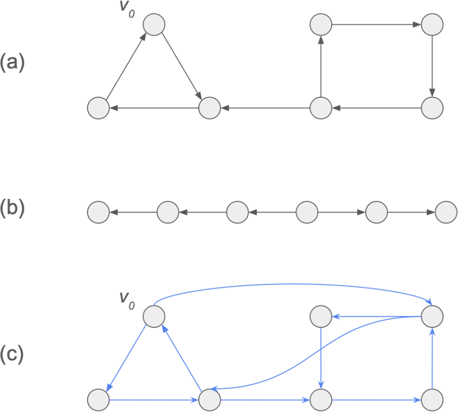


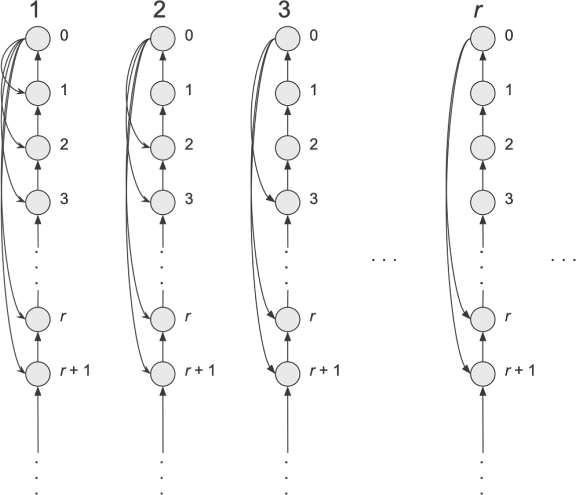


 Open access