


1 INTRODUCTION
Model misspecification is a major source of misleading inference in empirical work. This issue is further compounded when various competing models are available. It is thus imperative that model-based statistical inference be accompanied by proper model checks such as specification tests (Stute, Reference Stute1997).
Existing tests in the specification testing literature can be categorized into three classes, namely, conditional moment (CM) tests, nonparametric tests, and integrated CM (ICM) tests. The class of CM tests, such as those proposed by Newey (Reference Newey1985) and Tauchen (Reference Tauchen1985), is not consistent as it relies on only a finite number of moment conditions implied by the null hypothesis (Bierens, Reference Bierens1990). The class of nonparametric tests is therefore proposed as a remedy (see, e.g., Wooldridge, Reference Wooldridge1992; Yatchew, Reference Yatchew1992; Hardle and Mammen, Reference Hardle and Mammen1993; Hong and White, Reference Hong and White1995; Zheng, Reference Zheng1996; Li and Wang, Reference Li and Wang1998; Fan and Li, Reference Fan and Li2000; Su and White, Reference Su and White2007; Li, Liao, and Zhou, Reference Li, Liao and Zhou2026). The key idea of these test statistics is to nonparametrically estimate the CMs—such as through local smoothing techniques—and then compare them to their parametric counterparts under the null hypothesis.
The class of nonparametric tests may encounter challenges, such as nonparametric smoothing and suboptimal performance stemming from over-fitting the nonparametric alternative. In contrast, the class of ICM tests, such as those introduced by Bierens (Reference Bierens1982, Reference Bierens1990), Delgado (Reference Delgado1993), Bierens and Ploberger (Reference Bierens and Ploberger1997), Stute (Reference Stute1997), Delgado, Domínguez, and Lavergne (Reference Delgado, Domínguez and Lavergne2006), Escanciano (Reference Escanciano2006a), Domínguez and Lobato (Reference Domínguez and Lobato2015), Su and Zheng (Reference Su and Zheng2017), and Antoine and Lavergne (Reference Antoine and Lavergne2023), has gained popularity due to its ability to avoid these issues and detect local alternatives at faster rates. ICM metrics, on which ICM tests are based, also appear in other contexts: martingale difference hypothesis tests (Escanciano, Reference Escanciano2009a), joint coefficient and specification tests (Antoine and Lavergne, Reference Antoine and Lavergne2023), model-free feature screening (Zhu et al., Reference Zhu, Li, Li and Zhu2011; Shao and Zhang, Reference Shao and Zhang2014; Li et al., Reference Li, Ke, Yin and Yu2023), model estimation (Escanciano, Reference Escanciano2018; Tsyawo, Reference Tsyawo2023), specification tests of the propensity score (Sant’Anna and Song, Reference Sant’Anna and Song2019), and tests of the instrumental variable (IV) relevance condition in ICM estimators (Escanciano, Reference Escanciano2018; Tsyawo, Reference Tsyawo2023).
Despite their advantages, ICM tests are not widely used in empirical research (Escanciano, Reference Escanciano2009b; Domínguez and Lobato, Reference Domínguez and Lobato2015). First, ICM test statistics are not pivotal under the null hypothesis, thus critical values cannot be tabulated analytically (Bierens and Ploberger, Reference Bierens and Ploberger1997; Domínguez and Lobato, Reference Domínguez and Lobato2015). Second, ICM tests—when implemented via the wild bootstrap—tend to be computationally costly, as they require estimations on resampled data to compute p-values. Moreover, the wild bootstrap-based ICM test is arguably unsuitable for limited dependent outcome variable models such as logit, because bootstrap replicates of the outcome may fail to respect the outcome variable’s limited support. While the more recent multiplier bootstrap (MB) approach to ICM specification testing (e.g., Escanciano, Reference Escanciano2009b, Reference Escanciano2024; Li and Song, Reference Li and Song2022) offers a substantial computational advantage relative to the wild bootstrap by avoiding model re-estimation, it still entails non-negligible computational complexity due to re-sampling and the removal of the effect of estimating nuisance parameters. Third, although ICM tests are omnibus (Bierens, Reference Bierens1982; Stute, Reference Stute1997; Domínguez and Lobato, Reference Domínguez and Lobato2015), they only have substantial local power against alternatives in a finite-dimensional space (Escanciano, Reference Escanciano2009a). Moreover, it is not obvious how to leverage prior knowledge of potential directions under the alternative to enhance the power of existing ICM tests.
This article proposes a consistent $\chi ^2$
-test for the unified ICM framework of mean independence and specification testing. The key idea is to augment the ICM metric with a user-specified non-degenerate transformation of the conditioning covariates as in CM tests, which removes the first-order degeneracy inherent in classical ICM tests and yields a pivotal test statistic. The approach accommodates endogenous regressors, IVs, and heteroskedasticity of unknown form in both linear and non-linear models. As an ICM-based test, it is omnibus and capable of detecting a wide range of model misspecifications, including violations of IV exogeneity. Similar to the MB method (Escanciano, Reference Escanciano2009b), our approach is suited for models with possibly non-additively separable errors or non-continuous outcomes.
$\chi ^2$
-test for the unified ICM framework of mean independence and specification testing. The key idea is to augment the ICM metric with a user-specified non-degenerate transformation of the conditioning covariates as in CM tests, which removes the first-order degeneracy inherent in classical ICM tests and yields a pivotal test statistic. The approach accommodates endogenous regressors, IVs, and heteroskedasticity of unknown form in both linear and non-linear models. As an ICM-based test, it is omnibus and capable of detecting a wide range of model misspecifications, including violations of IV exogeneity. Similar to the MB method (Escanciano, Reference Escanciano2009b), our approach is suited for models with possibly non-additively separable errors or non-continuous outcomes.
Compared to existing ICM tests, our test has three advantages. First, it can be implemented as a $\chi ^2$
- or two-sided t-test, which can be interpreted more easily when compared to bootstrap-based tests. Second, the proposed test does not require bootstrap calibration of critical values; hence, it is computationally fast and remains feasible even in very large samples. Third, although our proposed test is not optimal, its power can be enhanced with the knowledge of directions under the alternative or, more generally, with directions the researcher may have in mind, whereas ICM tests lack this property. Therefore, we consider our test as a bridge between CM tests and ICM tests. We also acknowledge that the implementation of our test involves a tuning parameter, which is used in computing the generalized inverse that forms the Wald-type test statistic.
$\chi ^2$
- or two-sided t-test, which can be interpreted more easily when compared to bootstrap-based tests. Second, the proposed test does not require bootstrap calibration of critical values; hence, it is computationally fast and remains feasible even in very large samples. Third, although our proposed test is not optimal, its power can be enhanced with the knowledge of directions under the alternative or, more generally, with directions the researcher may have in mind, whereas ICM tests lack this property. Therefore, we consider our test as a bridge between CM tests and ICM tests. We also acknowledge that the implementation of our test involves a tuning parameter, which is used in computing the generalized inverse that forms the Wald-type test statistic.
This article is not the first attempt at circumventing the non-pivotality of ICM test statistics. Bierens (Reference Bierens1982) approximates the critical values of the ICM specification test using Chebyshev’s inequality for first moments under the null hypothesis, which is subsequently improved upon by Bierens and Ploberger (Reference Bierens and Ploberger1997). Bierens (Reference Bierens1982) also proposes a $\chi ^2$
-test based on two estimates of Fourier coefficients and a carefully chosen tuning parameter. Simulation evidence therein shows a high level of sensitivity to the tuning parameter. Besides, estimating Fourier coefficients no longer makes the test ICM as the test statistic is no longer “integrated.” Another attempt in the literature is the conditional Monte Carlo approach of De Jong (Reference De Jong1996) and Hansen (Reference Hansen1996). These are, however, computationally costly as Bierens and Ploberger (Reference Bierens and Ploberger1997) notes. Recent studies have also revisited the goal of constructing pivotal and computationally feasible specification tests within the CM framework. Raiola (Reference Raiola2024) draws inspiration from the classical Pearson’s
$\chi ^2$
-test based on two estimates of Fourier coefficients and a carefully chosen tuning parameter. Simulation evidence therein shows a high level of sensitivity to the tuning parameter. Besides, estimating Fourier coefficients no longer makes the test ICM as the test statistic is no longer “integrated.” Another attempt in the literature is the conditional Monte Carlo approach of De Jong (Reference De Jong1996) and Hansen (Reference Hansen1996). These are, however, computationally costly as Bierens and Ploberger (Reference Bierens and Ploberger1997) notes. Recent studies have also revisited the goal of constructing pivotal and computationally feasible specification tests within the CM framework. Raiola (Reference Raiola2024) draws inspiration from the classical Pearson’s $\chi ^2$
test by partitioning the sample space into cells. Although this test enjoys pivotality and excellent computational scalability, its power is inherently tied to the chosen partition and is therefore not fully omnibus: smooth model deviations that do not necessarily manifest as changes in constructed cells may go undetected. Li and Song (Reference Li and Song2025) leverage sample splitting and learn the optimal projection direction in the reproducing kernel Hilbert space via support vector machines (SVMs). This means that it can achieve high local power when the learned projection aligns with the alternative; however, sample splitting and hyperparameter tuning (in both kernels and SVM) may introduce finite-sample variability.
$\chi ^2$
test by partitioning the sample space into cells. Although this test enjoys pivotality and excellent computational scalability, its power is inherently tied to the chosen partition and is therefore not fully omnibus: smooth model deviations that do not necessarily manifest as changes in constructed cells may go undetected. Li and Song (Reference Li and Song2025) leverage sample splitting and learn the optimal projection direction in the reproducing kernel Hilbert space via support vector machines (SVMs). This means that it can achieve high local power when the learned projection aligns with the alternative; however, sample splitting and hyperparameter tuning (in both kernels and SVM) may introduce finite-sample variability.
The rest of the article is organized as follows. Section 2 provides a brief presentation of ICM metrics, a new metric, and its omnibus property. Section 3 proposes the $\chi ^2$
-test statistic and derives its limiting distribution under the null, local, and fixed alternative hypotheses within the unified framework of mean independence and specification tests. Monte Carlo simulations in Section 4 compare the empirical size and power of the
$\chi ^2$
-test statistic and derives its limiting distribution under the null, local, and fixed alternative hypotheses within the unified framework of mean independence and specification tests. Monte Carlo simulations in Section 4 compare the empirical size and power of the $ \chi ^2 $
specification test to the multiplier and wild bootstrap-based ICM specification tests, and Section 5 concludes. All technical proofs and additional simulation results are relegated to the Supplementary Material.
$ \chi ^2 $
specification test to the multiplier and wild bootstrap-based ICM specification tests, and Section 5 concludes. All technical proofs and additional simulation results are relegated to the Supplementary Material. $\textbf{Notation:} $
For
$\textbf{Notation:} $
For $a\in \mathbb {R}^p$
, we denote its transpose by
$a\in \mathbb {R}^p$
, we denote its transpose by $a^{\top }$
, and its Euclidean norm as
$a^{\top }$
, and its Euclidean norm as $\|a\|$
. We denote
$\|a\|$
. We denote $\mathrm {i}$
as the imaginary unit, which satisfies
$\mathrm {i}$
as the imaginary unit, which satisfies $\mathrm {i}^2=-1$
. “
$\mathrm {i}^2=-1$
. “ $\overset {p}{\rightarrow }$
” and “
$\overset {p}{\rightarrow }$
” and “ $\overset {d}{\rightarrow }$
” denote convergence in probability and distribution, respectively. Throughout the article, for a random vector W, we denote
$\overset {d}{\rightarrow }$
” denote convergence in probability and distribution, respectively. Throughout the article, for a random vector W, we denote $W^\dagger $
as its independent and identically distributed (
$W^\dagger $
as its independent and identically distributed ( $iid$
) copy, and write
$iid$
) copy, and write ${\mathbb {E}}_n W=n^{-1}\sum _{i=1}^n W_i$
as the empirical mean for
${\mathbb {E}}_n W=n^{-1}\sum _{i=1}^n W_i$
as the empirical mean for $iid$
copies
$iid$
copies $\{W_i\}_{i=1}^n$
of
$\{W_i\}_{i=1}^n$
of $W.$
To cut down on notational clutter,
$W.$
To cut down on notational clutter, $\widetilde {W}$
is sometimes used to denote the centered version of a random variable W, that is,
$\widetilde {W}$
is sometimes used to denote the centered version of a random variable W, that is, $\widetilde {W}:=W-{\mathbb {E}} W.$
2 THE FRAMEWORK
In this section, we briefly discuss ICM metrics, their omnibus property, and a new omnibus metric that characterizes mean independence.
2.1 ICM Metrics
For a random variable $U\in \mathbb {R}$
and a random vector
$U\in \mathbb {R}$
and a random vector $Z\in \mathbb {R}^{p_z},$
we say that U is mean-independent of Z, if
$Z\in \mathbb {R}^{p_z},$
we say that U is mean-independent of Z, if
 $$ \begin{align} {\mathbb{E}}[U \mid Z]={\mathbb{E}}[U] \ almost \ surely\ (a.s.), \end{align} $$
otherwise, U is mean-dependent on Z. To characterize the relationship (1), the existing literature puts much effort into studying ICM mean dependence metrics of the form:
 $$ \begin{align*} T(U \mid Z;\nu)=\int_{\Pi} \Big|{\mathbb{E}}[(U-{\mathbb{E}} U)w(s,Z)]\Big|^2\,\nu(ds), \end{align*} $$
where $w(s,Z)$
is a weight function indexed by
$w(s,Z)$
is a weight function indexed by $s \in \Pi $
, and
$s \in \Pi $
, and $\nu $
is a measure on
$\nu $
is a measure on $\Pi $
. A notable feature of
$\Pi $
. A notable feature of $T(U \mid Z;\nu )$
is its omnibus property, namely,
$T(U \mid Z;\nu )$
is its omnibus property, namely, $T(U \mid Z;\nu )=0$
if and only if (1) holds (see, e.g., Shao and Zhang, Reference Shao and Zhang2014, Thm. 1.2). The omnibus property guarantees the consistency of ICM tests. Therefore, a larger value of
$T(U \mid Z;\nu )=0$
if and only if (1) holds (see, e.g., Shao and Zhang, Reference Shao and Zhang2014, Thm. 1.2). The omnibus property guarantees the consistency of ICM tests. Therefore, a larger value of ${T(U \mid Z;\nu )}$
indicates a stronger mean dependence of U on Z.
${T(U \mid Z;\nu )}$
indicates a stronger mean dependence of U on Z.
Under suitable conditions, the ICM metric has the general form:
 $$ \begin{align*} T(U \mid Z;\nu) &= \int_{\Pi} \Big({\mathbb{E}}[(U-{\mathbb{E}} U)w(s,Z)]\Big)\overline{\Big({\mathbb{E}}[(U-{\mathbb{E}} U)w(s,Z)]\Big)}\nu(ds)\\ &= {\mathbb{E}}\Big[(U-{\mathbb{E}} U)(U^\dagger-{\mathbb{E}} U)\int_{\Pi} \big(w(s,Z)\overline{w(s,Z^\dagger)}\big)\nu(ds) \Big]\\ &:= {\mathbb{E}}\Big[(U-{\mathbb{E}} U)(U^\dagger-{\mathbb{E}} U)K(Z,Z^\dagger)\Big]\\ &:= \mathrm{ICM}(U \mid Z), \end{align*} $$
where $\overline {w(\cdot ,\cdot )}$
denotes the complex conjugate of
$\overline {w(\cdot ,\cdot )}$
denotes the complex conjugate of $w(\cdot ,\cdot )$
and
$w(\cdot ,\cdot )$
and $K(\cdot ,\cdot )$
denotes the kernel. Table 1 provides a few examples of commonly used ICM kernels (see Li et al., Reference Li, Ke, Yin and Yu2023 for a recent review).
$K(\cdot ,\cdot )$
denotes the kernel. Table 1 provides a few examples of commonly used ICM kernels (see Li et al., Reference Li, Ke, Yin and Yu2023 for a recent review).
Examples of ICM kernels

Note: $\phi (x) = \frac {1}{\sqrt {2\pi }} e^{-\frac {1}{2}x^2} $
is the standard normal probability density function, and
$\phi (x) = \frac {1}{\sqrt {2\pi }} e^{-\frac {1}{2}x^2} $
is the standard normal probability density function, and $ c_p = \frac {\pi ^{(1+p)/2}}{\Gamma ((1+p)/2)}, \ p \geq 1, $
where
$ c_p = \frac {\pi ^{(1+p)/2}}{\Gamma ((1+p)/2)}, \ p \geq 1, $
where $ \Gamma (\cdot ) $
is the complete gamma function.
$ \Gamma (\cdot ) $
is the complete gamma function.
Examples of weight functions from the literature include the step function $w(s,Z) = \mathrm {I}(Z\leq s) $
(e.g., Stute, Reference Stute1997; Domínguez and Lobato, Reference Domínguez and Lobato2004; Delgado et al., Reference Delgado, Domínguez and Lavergne2006; Escanciano, Reference Escanciano2006b; Zhu et al., Reference Zhu, Li, Li and Zhu2011); a one-dimensional projection in the step function
$w(s,Z) = \mathrm {I}(Z\leq s) $
(e.g., Stute, Reference Stute1997; Domínguez and Lobato, Reference Domínguez and Lobato2004; Delgado et al., Reference Delgado, Domínguez and Lavergne2006; Escanciano, Reference Escanciano2006b; Zhu et al., Reference Zhu, Li, Li and Zhu2011); a one-dimensional projection in the step function $w(s,Z) =\mathrm {I}(Z^{\top }s_{-1}\leq s_1)$
(e.g., Escanciano, Reference Escanciano2006a; Kim, Balakrishnan, and Wasserman, Reference Kim, Balakrishnan and Wasserman2020); the real exponential
$w(s,Z) =\mathrm {I}(Z^{\top }s_{-1}\leq s_1)$
(e.g., Escanciano, Reference Escanciano2006a; Kim, Balakrishnan, and Wasserman, Reference Kim, Balakrishnan and Wasserman2020); the real exponential $w(s,Z) = \exp (Z^{\top }s)$
(e.g., Bierens, Reference Bierens1990); and the complex exponential
$w(s,Z) = \exp (Z^{\top }s)$
(e.g., Bierens, Reference Bierens1990); and the complex exponential $w(s,Z)=\exp (\mathrm {i}Z^{\top }s)$
(e.g., Bierens (Reference Bierens1982), Shao and Zhang (Reference Shao and Zhang2014), and Antoine and Lavergne (Reference Antoine and Lavergne2023)). The space
$w(s,Z)=\exp (\mathrm {i}Z^{\top }s)$
(e.g., Bierens (Reference Bierens1982), Shao and Zhang (Reference Shao and Zhang2014), and Antoine and Lavergne (Reference Antoine and Lavergne2023)). The space $\Pi $
in Escanciano (Reference Escanciano2006a) and Kim et al. (Reference Kim, Balakrishnan and Wasserman2020) is given by
$\Pi $
in Escanciano (Reference Escanciano2006a) and Kim et al. (Reference Kim, Balakrishnan and Wasserman2020) is given by $\Pi = \mathbb {R}\times \mathbb {S}_{p_z}$
, where
$\Pi = \mathbb {R}\times \mathbb {S}_{p_z}$
, where $\mathbb {S}_{p_z}$
denotes the space of
$\mathbb {S}_{p_z}$
denotes the space of $p_z\times 1$
vectors with unit Euclidean norm while
$p_z\times 1$
vectors with unit Euclidean norm while $\Pi =\mathbb {R}^{p_z}$
for the other works mentioned above. See Escanciano (Reference Escanciano2006b, Lemma 1) for a general characterization of ICM weight functions.
$\Pi =\mathbb {R}^{p_z}$
for the other works mentioned above. See Escanciano (Reference Escanciano2006b, Lemma 1) for a general characterization of ICM weight functions.
The omnibus property of ICM metrics thus translates as
 $$ \begin{align} \mathrm{ICM}(U \mid Z)=0 \quad \text{if and only if }~~ {\mathbb{E}}[U \mid Z]={\mathbb{E}}[U] \ almost \ surely \ (a.s). \end{align} $$
When $ U $
and
$ U $
and $ Z $
are observed, a natural empirical estimator of
$ Z $
are observed, a natural empirical estimator of $ \mathrm {ICM}(U \mid Z) $
is given by the (modified) U-statistic
$ \mathrm {ICM}(U \mid Z) $
is given by the (modified) U-statistic
 $$ \begin{align*} \widehat{\mathrm{ICM}}_n(U \mid Z) = \frac{1}{n(n-1)} \sum_{i \neq j} (U_i - {\mathbb{E}}_n[U])(U_j - {\mathbb{E}}_n[U]) K(Z_i, Z_j). \end{align*} $$
As with most existing ICM-based tests, the asymptotic null distribution of the corresponding test statistic (under (1)) is non-pivotal (Bierens and Ploberger, Reference Bierens and Ploberger1997, Thm. 3):
 $$ \begin{align} n\widehat{\mathrm{ICM}}_n(U \mid Z) \overset{d}{\rightarrow} \sum_{k=1}^{\infty}\lambda_k G_k^2, \end{align} $$
granted ${\mathbb {E}} [U^2U^{\dagger 2}K^2(Z,Z^{\dagger })]<\infty $
. Here,
${\mathbb {E}} [U^2U^{\dagger 2}K^2(Z,Z^{\dagger })]<\infty $
. Here, $\{G_k\}_{k=1}^{\infty }$
is a sequence of
$\{G_k\}_{k=1}^{\infty }$
is a sequence of $iid$
standard Gaussian random variables, and
$iid$
standard Gaussian random variables, and $\{\lambda _k\}_{k=1}^{\infty }, \ \lambda _k\geq 0$
, is a sequence of non-increasing coefficients that depend on the distribution of
$\{\lambda _k\}_{k=1}^{\infty }, \ \lambda _k\geq 0$
, is a sequence of non-increasing coefficients that depend on the distribution of $[U,Z^\top ]^\top $
and the kernel
$[U,Z^\top ]^\top $
and the kernel $K(\cdot ,\cdot )$
. Thus, the limiting distribution of
$K(\cdot ,\cdot )$
. Thus, the limiting distribution of $ n\widehat {\mathrm {ICM}}_n(U \mid Z) $
under (1) is non-pivotal, and re-sampling/bootstrap techniques are usually required to obtain valid
$ n\widehat {\mathrm {ICM}}_n(U \mid Z) $
under (1) is non-pivotal, and re-sampling/bootstrap techniques are usually required to obtain valid $ p $
-values for inference.
$ p $
-values for inference.
2.2 A New Characterization of Mean Independence
Consider the following test hypotheses of mean independence:
 $$ \begin{align} \begin{aligned} \mathbb{H}_o&: {\mathbb{E}}[U \mid Z] - {\mathbb{E}}[U] = 0 \ a.s.; \\ \mathbb{H}_a&: \mathbb{P}\big({\mathbb{E}}[U \mid Z]={\mathbb{E}}[U]\big) < 1. \end{aligned} \end{align} $$
The above hypotheses of interest, in view of the omnibus property (2), can be restated as testing $ \mathrm {ICM}(U \mid Z)=0.$
Indeed, by the law of iterated expectations (LIE),
$ \mathrm {ICM}(U \mid Z)=0.$
Indeed, by the law of iterated expectations (LIE),
 $$ \begin{align} \begin{aligned} \mathrm{ICM}(U \mid Z)=&\ {\mathbb{E}}\left\{K(Z,Z^\dagger) (U^\dagger-{\mathbb{E}} U) {\mathbb{E}}[(U-{\mathbb{E}} U) \mid Z,Z^\dagger,U^\dagger]\right\} \\ =&\ {\mathbb{E}}\left\{K(Z,Z^\dagger)(\underbrace{{\mathbb{E}}[U \mid Z]-{\mathbb{E}} U}_{=\,0 \, a.s. \text{ under } \mathbb{H}_o})(U^\dagger-{\mathbb{E}} U)\right\}. \end{aligned} \end{align} $$
Under $\mathbb {H}_o$
,
$\mathbb {H}_o$
, ${\mathbb {E}}[U \mid Z]$
is degenerate, that is,
${\mathbb {E}}[U \mid Z]$
is degenerate, that is, ${\mathbb {E}}[U \mid Z]-{\mathbb {E}} U=0\ a.s.$
This is the first-order degeneracy problem in U/V-statistic-based estimator for (5) that accounts for the non-pivotal limiting distribution in (3). In this regard, we propose to replace the role of U in the ICM metric with a random vector
${\mathbb {E}}[U \mid Z]-{\mathbb {E}} U=0\ a.s.$
This is the first-order degeneracy problem in U/V-statistic-based estimator for (5) that accounts for the non-pivotal limiting distribution in (3). In this regard, we propose to replace the role of U in the ICM metric with a random vector $V\in \mathbb {R}^{p_v}$
constructed such that
$V\in \mathbb {R}^{p_v}$
constructed such that ${\mathbb {E}}[V \mid Z]$
is non-degenerate under both the null and alternative hypotheses while preserving the omnibus property (2). In other words, we propose to measure the mean independence of U on Z with the assistance of a random vector V by
${\mathbb {E}}[V \mid Z]$
is non-degenerate under both the null and alternative hypotheses while preserving the omnibus property (2). In other words, we propose to measure the mean independence of U on Z with the assistance of a random vector V by
 $$ \begin{align*}\delta(V):= {\mathbb{E}}\left[K(Z,Z^\dagger) (U^\dagger-{\mathbb{E}} U) (V - {\mathbb{E}} V) \right]. \end{align*} $$
The resulting test relies on the empirical estimator of $\delta (V)$
.
$\delta (V)$
.
The two key properties—first-order non-degeneracy and omnibusness—ensure a pivotal limiting distribution under the null and the consistency of the test, respectively. Specifically, we require (1) V to be mean dependent on Z to rule out first-order degeneracy and (2) V to be chosen such that $\delta (V)\neq 0$
under
$\delta (V)\neq 0$
under $\mathbb {H}_a$
. The first condition is easy to satisfy by selecting V to be a measurable function of Z. In contrast, the second condition is non-trivial: randomly selecting V may lead to the same limitation as the classical CM test if it happens to be orthogonal to the direction of departure under
$\mathbb {H}_a$
. The first condition is easy to satisfy by selecting V to be a measurable function of Z. In contrast, the second condition is non-trivial: randomly selecting V may lead to the same limitation as the classical CM test if it happens to be orthogonal to the direction of departure under $\mathbb {H}_a$
. This trade-off mirrors the strengths and weaknesses of existing methods: while the CM test is first-order non-degenerate, it may lack consistency under
$\mathbb {H}_a$
. This trade-off mirrors the strengths and weaknesses of existing methods: while the CM test is first-order non-degenerate, it may lack consistency under $\mathbb {H}_a$
; conversely, the ICM test is consistent under
$\mathbb {H}_a$
; conversely, the ICM test is consistent under $\mathbb {H}_a$
, but suffers from first-order degeneracy, resulting in a non-pivotal limiting distribution under
$\mathbb {H}_a$
, but suffers from first-order degeneracy, resulting in a non-pivotal limiting distribution under $\mathbb {H}_o$
.
$\mathbb {H}_o$
.
To this end, the proposed testing procedure integrates the respective strengths of two existing approaches in the literature: the pivotality of the CM test and the omnibus property of the ICM test. In particular, we focus on the quantity
 $$ \begin{align} V_h = \big[ h(Z), \ U - h(Z) \big]^\top, \end{align} $$
such that
 $$ \begin{align} \delta_h:=\delta(V_h)= \begin{bmatrix} {\mathbb{E}}[K(Z,Z^\dagger) (h(Z)-{\mathbb{E}}[h(Z)]) ({U}^\dagger-{\mathbb{E}} U)]\\ \mathrm{ICM}(U \mid Z) - {\mathbb{E}}[K(Z,Z^\dagger) (h(Z)-{\mathbb{E}}[h(Z)]) ({U}^\dagger-{\mathbb{E}} U)] \end{bmatrix}. \end{align} $$
The two components in $V_h$
, namely,
$V_h$
, namely, $h(Z)$
and
$h(Z)$
and $U - h(Z) $
, serve different purposes. First, one can view
$U - h(Z) $
, serve different purposes. First, one can view $h(Z)$
as the assistant function where prior information about the alternative can be incorporated, as done in the classical CM test. Second, the inclusion of
$h(Z)$
as the assistant function where prior information about the alternative can be incorporated, as done in the classical CM test. Second, the inclusion of $ U $
in the second element draws inspiration from ICM tests, which gives the omnibus property of our test, that is, it has non-trivial power in all possible directions of the alternative. This structure acts as a safeguard in scenarios where the chosen assistant
$ U $
in the second element draws inspiration from ICM tests, which gives the omnibus property of our test, that is, it has non-trivial power in all possible directions of the alternative. This structure acts as a safeguard in scenarios where the chosen assistant $h(Z)$
is (nearly) orthogonal to the alternative, a situation in which traditional CM tests suffer from trivial power. Moreover, the
$h(Z)$
is (nearly) orthogonal to the alternative, a situation in which traditional CM tests suffer from trivial power. Moreover, the $-h(Z)$
in the second element ensures that
$-h(Z)$
in the second element ensures that $\delta _h$
is first-order non-degenerate and that the proposed test statistic is pivotal (
$\delta _h$
is first-order non-degenerate and that the proposed test statistic is pivotal ( $\chi ^2$
-distributed) under the null hypothesis. We remark that the choice of V can be readily extended beyond two dimensions, although in this article, we focus on the specific two-dimensional case for clarity and analytical tractability.
$\chi ^2$
-distributed) under the null hypothesis. We remark that the choice of V can be readily extended beyond two dimensions, although in this article, we focus on the specific two-dimensional case for clarity and analytical tractability.
The following fundamental result establishes the omnibus and first-order non-degeneracy properties of $\delta _h $
.
$\delta _h $
.
Lemma 2.1. Let $ h(Z) $
denote an arbitrary measurable and non-degenerate function of Z, in the sense that
$ h(Z) $
denote an arbitrary measurable and non-degenerate function of Z, in the sense that $ \mathbb {P}\big ( h(Z) = \mathbb {E}[h(Z)] \big ) < 1 $
. Then: (a)
$ \mathbb {P}\big ( h(Z) = \mathbb {E}[h(Z)] \big ) < 1 $
. Then: (a) $ \delta _h $
defined in (7) satisfies the omnibus property, that is,
$ \delta _h $
defined in (7) satisfies the omnibus property, that is, $ \|\delta _h\| = 0 $
if and only if (2) holds and (b)
$ \|\delta _h\| = 0 $
if and only if (2) holds and (b) $ \delta _h $
exhibits first-order non-degeneracy.
$ \delta _h $
exhibits first-order non-degeneracy.
Proof. Let $\delta _h^{(1)}={\mathbb {E}}[K(Z,Z^{\dagger })(h(Z) - {\mathbb {E}}[h(Z)])({U}^\dagger -{\mathbb {E}} U)]$
and
$\delta _h^{(1)}={\mathbb {E}}[K(Z,Z^{\dagger })(h(Z) - {\mathbb {E}}[h(Z)])({U}^\dagger -{\mathbb {E}} U)]$
and $\delta _h^{(2)}=\mathrm {ICM}(U \mid Z)-\delta _h^{(1)}$
. Then, from (7), we have that
$\delta _h^{(2)}=\mathrm {ICM}(U \mid Z)-\delta _h^{(1)}$
. Then, from (7), we have that $\delta _h=[\delta _h^{(1)},\delta _h^{({2})}]^{\top }$
and
$\delta _h=[\delta _h^{(1)},\delta _h^{({2})}]^{\top }$
and $\delta _h^{(1)} + \delta _h^{(2)} = \mathrm {ICM}(U \mid Z)> 0$
under
$\delta _h^{(1)} + \delta _h^{(2)} = \mathrm {ICM}(U \mid Z)> 0$
under $\mathbb {H}_a$
. This implies that under
$\mathbb {H}_a$
. This implies that under $\mathbb {H}_a$
, at least one element in
$\mathbb {H}_a$
, at least one element in $\delta _h$
is strictly positive (hence strictly different from zero);
$\delta _h$
is strictly positive (hence strictly different from zero); $\delta _h$
satisfies the omnibus property. Note that
$\delta _h$
satisfies the omnibus property. Note that $h(Z)$
is non-degenerate, and that under
$h(Z)$
is non-degenerate, and that under $\mathbb {H}_o$
,
$\mathbb {H}_o$
, ${\mathbb {E}} \big [V_h - {\mathbb {E}}[V_h] \mid Z\big ] = \big [(h(Z) - {\mathbb {E}}[h(Z)]),\ {\mathbb {E}} [U \mid Z] - {\mathbb {E}} U - (h(Z) - {\mathbb {E}}[h(Z)]) \big ]^{\top } = (h(Z) - {\mathbb {E}}[h(Z)])[1,-1]^{\top }\neq 0 $
with probability one. It follows that
${\mathbb {E}} \big [V_h - {\mathbb {E}}[V_h] \mid Z\big ] = \big [(h(Z) - {\mathbb {E}}[h(Z)]),\ {\mathbb {E}} [U \mid Z] - {\mathbb {E}} U - (h(Z) - {\mathbb {E}}[h(Z)]) \big ]^{\top } = (h(Z) - {\mathbb {E}}[h(Z)])[1,-1]^{\top }\neq 0 $
with probability one. It follows that $\delta _h$
avoids first-order degeneracy.
$\delta _h$
avoids first-order degeneracy.
Lemma 2.1 implies that, with our construction of $V_h$
in (6),
$V_h$
in (6), $\delta _h$
is nonzero under the alternative. Therefore,
$\delta _h$
is nonzero under the alternative. Therefore, $\|\delta _h\|$
can be interpreted as a metric for conditional mean independence, that is,
$\|\delta _h\|$
can be interpreted as a metric for conditional mean independence, that is, $\|\delta _h\|=0$
if and only if
$\|\delta _h\|=0$
if and only if $\mathbb {E}[U\mid Z]=\mathbb {E}[U] \ a.s. $
While the performance of
$\mathbb {E}[U\mid Z]=\mathbb {E}[U] \ a.s. $
While the performance of $\delta _h$
depends on the choice of
$\delta _h$
depends on the choice of $h(\cdot )$
, we note that similar concerns arise in ICM tests, particularly regarding the selection of kernels. A practitioner who is agnostic about the alternative can use
$h(\cdot )$
, we note that similar concerns arise in ICM tests, particularly regarding the selection of kernels. A practitioner who is agnostic about the alternative can use ![]() , where
, where ![]() denotes a
denotes a $p\times 1$
vector of ones.Footnote
1
The Maclaurin’s series expansion, namely,
$p\times 1$
vector of ones.Footnote
1
The Maclaurin’s series expansion, namely, $\exp (z) = \sum _{l=0}^{\infty } z^l/{l!}$
shows the potential of
$\exp (z) = \sum _{l=0}^{\infty } z^l/{l!}$
shows the potential of ![]() to capture different directions under the alternative.Footnote
2
to capture different directions under the alternative.Footnote
2
A key message of Lemma 2.1 is that symmetrizing any non-degenerate measurable function $h(\cdot )$
of Z about U guarantees the omnibus and first-order non-degeneracy properties of
$h(\cdot )$
of Z about U guarantees the omnibus and first-order non-degeneracy properties of $\delta _h$
. The requirement on
$\delta _h$
. The requirement on $h(Z)$
in Lemma 2.1 can hardly be termed a “condition,” as it imposes only measurability and non-degeneracy. The proof of Lemma 2.1 provides an insight into the inclusion of U linearly in the construction of V. This brings in the term
$h(Z)$
in Lemma 2.1 can hardly be termed a “condition,” as it imposes only measurability and non-degeneracy. The proof of Lemma 2.1 provides an insight into the inclusion of U linearly in the construction of V. This brings in the term $\mathrm {ICM}(U \mid Z)$
in
$\mathrm {ICM}(U \mid Z)$
in $\delta _h$
that is strictly positive under
$\delta _h$
that is strictly positive under $\mathbb {H}_a$
and contributes power under the alternative. The proposed test thus draws its consistency from the ICM metric.
$\mathbb {H}_a$
and contributes power under the alternative. The proposed test thus draws its consistency from the ICM metric.
Since $h(Z)$
can be chosen arbitrarily, the practitioner does not bear the burden of “carefully” selecting functions such as polynomials that provide power by approximating
$h(Z)$
can be chosen arbitrarily, the practitioner does not bear the burden of “carefully” selecting functions such as polynomials that provide power by approximating ${\mathbb {E}}[U \mid Z]$
under
${\mathbb {E}}[U \mid Z]$
under $\mathbb {H}_a$
, as required in nonparametric specification tests (e.g., Wooldridge, Reference Wooldridge1992; Yatchew, Reference Yatchew1992; Zheng, Reference Zheng1996). In addition, the user-specified
$\mathbb {H}_a$
, as required in nonparametric specification tests (e.g., Wooldridge, Reference Wooldridge1992; Yatchew, Reference Yatchew1992; Zheng, Reference Zheng1996). In addition, the user-specified $h(Z)$
provides extra flexibility as the practitioner can use it to augment the power of the test in given directions, unlike existing ICM-based bootstrap tests.
$h(Z)$
provides extra flexibility as the practitioner can use it to augment the power of the test in given directions, unlike existing ICM-based bootstrap tests.
Remark 2.1. We assume that $p_z$
is fixed in this study. In high-dimensional settings where
$p_z$
is fixed in this study. In high-dimensional settings where $p_z \rightarrow \infty $
, Zhang et al. (Reference Zhang, Yao and Shao2018, Remark 2.2) demonstrate that
$p_z \rightarrow \infty $
, Zhang et al. (Reference Zhang, Yao and Shao2018, Remark 2.2) demonstrate that $\mathrm {ICM}$
criteria only capture linear dependence. Our
$\mathrm {ICM}$
criteria only capture linear dependence. Our $\chi ^2$
-test derives its consistency property and part of its power from the
$\chi ^2$
-test derives its consistency property and part of its power from the $\mathrm {ICM}$
metric so it cannot be expected to perform better in high dimensions. Recent studies have explored the challenge of testing independence between high-dimensional random vectors using distance covariance-based statistics (Székely, Rizzo, and Bakirov, Reference Székely, Rizzo and Bakirov2007), revealing that the performance of such tests depends critically on the relative growth rates of the dimensions of the random variables and the sample size n (Zhu et al., Reference Zhu, Zhang, Yao and Shao2020; Chakraborty and Zhang, Reference Chakraborty and Zhang2021; Gao et al., Reference Gao, Fan, Lv and Shao2021; Zhang, Zhang, and Zhou, Reference Zhang, Zhang and Zhou2023). Consequently, extending the current testing procedure to high dimensions requires a separate study that is deferred to future research.
$\mathrm {ICM}$
metric so it cannot be expected to perform better in high dimensions. Recent studies have explored the challenge of testing independence between high-dimensional random vectors using distance covariance-based statistics (Székely, Rizzo, and Bakirov, Reference Székely, Rizzo and Bakirov2007), revealing that the performance of such tests depends critically on the relative growth rates of the dimensions of the random variables and the sample size n (Zhu et al., Reference Zhu, Zhang, Yao and Shao2020; Chakraborty and Zhang, Reference Chakraborty and Zhang2021; Gao et al., Reference Gao, Fan, Lv and Shao2021; Zhang, Zhang, and Zhou, Reference Zhang, Zhang and Zhou2023). Consequently, extending the current testing procedure to high dimensions requires a separate study that is deferred to future research.
2.3 Extension to Testing the Nullity of ${\mathbb {E}}[U \mid Z]$

In some applications, such as specification testing, one may be interested in the almost sure nullity of ${\mathbb {E}}[U \mid Z]$
directly, that is,
${\mathbb {E}}[U \mid Z]$
directly, that is,
 $$ \begin{align} \mathbb{H}_o^*&: {\mathbb{E}}[U \mid Z]=0 \ a.s.; \quad \mathbb{H}_a^* : \mathbb{P}({\mathbb{E}}[U \mid Z]=0) <1. \end{align} $$
This is an augmented version of (4) which further imposes ${\mathbb {E}}[U]=0$
, that is, a joint hypothesis of conditional mean independence and nullity of the unconditional mean. To this end, we follow Su and Zheng (Reference Su and Zheng2017) by augmenting
${\mathbb {E}}[U]=0$
, that is, a joint hypothesis of conditional mean independence and nullity of the unconditional mean. To this end, we follow Su and Zheng (Reference Su and Zheng2017) by augmenting $\delta _h$
with an additional quantity that accounts for
$\delta _h$
with an additional quantity that accounts for ${\mathbb {E}}[U] = 0$
under
${\mathbb {E}}[U] = 0$
under $\mathbb {H}_o^*$
. In particular, one may consider the metric
$\mathbb {H}_o^*$
. In particular, one may consider the metric
 $$ \begin{align*}\delta_h^*=\delta_h + {\mathbb{E}}|K(Z,Z^{\dagger})|{\mathbb{E}} U {\mathbb{E}}\big[h(Z), \ U - h(Z)) \big]^\top. \end{align*} $$
The following result shows that ${\delta }_h^*$
has the omnibus property with respect to (8).
${\delta }_h^*$
has the omnibus property with respect to (8).
Lemma 2.2. ${\delta }_h^*=0$
if and only if
${\delta }_h^*=0$
if and only if ${\mathbb {E}}[U \mid Z]=0 \ a.s. $
To conserve space, the discussion below focuses on $\delta _h$
. Theoretical properties of the
$\delta _h$
. Theoretical properties of the $\chi ^2$
-test based on
$\chi ^2$
-test based on $\delta _h^*$
are presented in Section S.3 of the Supplementary Material.
$\delta _h^*$
are presented in Section S.3 of the Supplementary Material.
3 TEST STATISTIC AND THEORETICAL PROPERTIES
In this section, we construct the test statistic based on $\delta _h$
. In Section 3.1, we present a framework that unifies the tests of mean independence and model specification. We analyze the asymptotic behavior of
$\delta _h$
. In Section 3.1, we present a framework that unifies the tests of mean independence and model specification. We analyze the asymptotic behavior of $\widehat {\delta }_h$
, the empirical estimator for
$\widehat {\delta }_h$
, the empirical estimator for $\delta _h$
, and the
$\delta _h$
, and the $\chi ^2$
-distributed test statistic under the null hypothesis, as well as under local and fixed alternatives in Sections 3.2 and 3.3, respectively. Section 3.4 uses Bahadur slopes to compare the power of the
$\chi ^2$
-distributed test statistic under the null hypothesis, as well as under local and fixed alternatives in Sections 3.2 and 3.3, respectively. Section 3.4 uses Bahadur slopes to compare the power of the $\chi ^2$
-test and bootstrap-based
$\chi ^2$
-test and bootstrap-based $\mathrm {ICM}$
tests.
$\mathrm {ICM}$
tests.
3.1 A Unified Framework
The mean independence testing problem and the specification testing problem are two closely related problems in econometric analyses. Here, we present a unified framework for both tasks. Let $X\in \mathbb {R}^{p_x}$
and
$X\in \mathbb {R}^{p_x}$
and $Z\in \mathbb {R}^{p_z}$
be two random vectors. We consider an econometric model defined by the following CM restriction:
$Z\in \mathbb {R}^{p_z}$
be two random vectors. We consider an econometric model defined by the following CM restriction:
 $$ \begin{align} \mathbb{E}[U(X;\theta_o)|Z]=0\quad a.s., \end{align} $$
for a unique model parameter $\theta _o\in \Theta \subset \mathbb {R}^k$
. Here,
$\theta _o\in \Theta \subset \mathbb {R}^k$
. Here, $U:\mathbb {R}^{p_x}\times \Theta \mapsto \mathbb {R}^{p_u}$
is the econometric model that is assumed to be known, and
$U:\mathbb {R}^{p_x}\times \Theta \mapsto \mathbb {R}^{p_u}$
is the econometric model that is assumed to be known, and $\Theta $
is the parameter space. Given
$\Theta $
is the parameter space. Given $iid$
observations
$iid$
observations $\{X_i,Z_i\}_{i=1}^n$
, and an empirical estimator
$\{X_i,Z_i\}_{i=1}^n$
, and an empirical estimator $\widehat {\theta }_n$
for
$\widehat {\theta }_n$
for $\theta _o$
, we are interested in assessing the model specification in (9).
$\theta _o$
, we are interested in assessing the model specification in (9).
The above framework encompasses a wide range of applications, including treatment effect analyses (e.g., Sant’Anna and Song, Reference Sant’Anna and Song2019; Callaway and Karami, Reference Callaway and Karami2023), Euler and Bellman equations (Hansen and Singleton, Reference Hansen and Singleton1982; Escanciano, Reference Escanciano2018), the hybrid New Keynesian Phillips curve (Choi, Escanciano, and Guo, Reference Choi, Escanciano and Guo2022), forecast rationality (Hansen and Hodrick, Reference Hansen and Hodrick1980), and tests of conditional equal and predictive ability (Giacomini and White, Reference Giacomini and White2006) (see Li et al., Reference Li, Liao and Zhou2026 for a comprehensive discussion).
In the mean independence testing problem outlined in Section 2.2, the expressions for $ \mathrm {ICM}(U \mid Z) $
and
$ \mathrm {ICM}(U \mid Z) $
and $ \delta _h $
involve the nuisance parameter
$ \delta _h $
involve the nuisance parameter $ \mathbb {E} U $
. In this case, we can simply set
$ \mathbb {E} U $
. In this case, we can simply set $X=U$
,
$X=U$
, $\theta _o=\mathbb {E}U$
, and
$\theta _o=\mathbb {E}U$
, and $U(X;\theta )=X-\theta $
, then testing for (9) reduces to the hypothesis (4). In the class of nonlinear models with additively separable errors
$U(X;\theta )=X-\theta $
, then testing for (9) reduces to the hypothesis (4). In the class of nonlinear models with additively separable errors $X^{(1)} = g(X^{(-1)};\beta _o) + U $
, where
$X^{(1)} = g(X^{(-1)};\beta _o) + U $
, where $X^{(1)}$
denotes the first element of X,
$X^{(1)}$
denotes the first element of X, $X^{(-1)}$
is the sub-vector of X that excludes
$X^{(-1)}$
is the sub-vector of X that excludes $X^{(1)}$
, and U is the model error (up to a location shift), we let
$X^{(1)}$
, and U is the model error (up to a location shift), we let
 $$ \begin{align*} U(X;\theta) &= X^{(1)} - g(X^{(-1)};\beta) - \theta_c, \end{align*} $$
where $\theta = [ \theta _c,\ \beta ^\top ]^\top $
, and
$\theta = [ \theta _c,\ \beta ^\top ]^\top $
, and $\theta _c$
is the location parameter such that
$\theta _c$
is the location parameter such that $\mathbb {E}[X_1-g(X_{-1};\beta )-U]=\theta _c$
. Including the location parameter
$\mathbb {E}[X_1-g(X_{-1};\beta )-U]=\theta _c$
. Including the location parameter $\theta _c$
in
$\theta _c$
in $\theta $
becomes necessary as the ICM metric and
$\theta $
becomes necessary as the ICM metric and $\delta _h$
can only identify mean independence up to an unknown nuisance mean shift. Nullity testing is discussed in Section 2.3.
$\delta _h$
can only identify mean independence up to an unknown nuisance mean shift. Nullity testing is discussed in Section 2.3.
In practice, a natural estimator for $\delta _h$
in (7) is given by
$\delta _h$
in (7) is given by
 $$ \begin{align} \widehat{\delta}_h& = \frac{1}{n(n-1)}\sum_{i=1}^n\sum_{j\neq i}K(Z_i,Z_j)U(X_i;\widehat{\theta}_n)\nonumber\\&\quad\big[(h(Z_j) - {\mathbb{E}}_n[h(Z)]) , \ U(X_j;\widehat{\theta}_n) - (h(Z_j) - {\mathbb{E}}_n[h(Z)]) \big]^\top. \end{align} $$
We remark that, for the mean independence testing problem in (4), $U(X_i;\widehat {\theta }_n)=U_i-\widehat {\theta }_n$
with
$U(X_i;\widehat {\theta }_n)=U_i-\widehat {\theta }_n$
with $\widehat {\theta }_n={\mathbb {E}}_nU.$
3.2 Asymptotic Distribution
In this section, we analyze the asymptotic behavior of $ \widehat {\delta }_h $
under the null hypothesis, local alternatives, and fixed alternatives. Let
$ \widehat {\delta }_h $
under the null hypothesis, local alternatives, and fixed alternatives. Let $ D := [U, X^\top , Z^\top ]^\top $
, and define
$ D := [U, X^\top , Z^\top ]^\top $
, and define $ \widetilde {U} := U(X; \theta _o) $
such that
$ \widetilde {U} := U(X; \theta _o) $
such that ${\mathbb {E}}\widetilde {U}=0.$
We consider the following sequences of local alternatives: Pitman local alternatives
${\mathbb {E}}\widetilde {U}=0.$
We consider the following sequences of local alternatives: Pitman local alternatives $ \mathbb {H}_{an}: \mathbb {E}[\widetilde {U} \mid Z] = n^{-1/2} a(Z)$
and milder (non-Pitman) local alternatives
$ \mathbb {H}_{an}: \mathbb {E}[\widetilde {U} \mid Z] = n^{-1/2} a(Z)$
and milder (non-Pitman) local alternatives $ \mathbb {H}_{an}': \mathbb {E}[\widetilde {U} \mid Z] = n^{-1/4} a(Z) $
, where
$ \mathbb {H}_{an}': \mathbb {E}[\widetilde {U} \mid Z] = n^{-1/4} a(Z) $
, where $ a(Z) $
is a non-degenerate measurable function of
$ a(Z) $
is a non-degenerate measurable function of $ Z $
satisfying
$ Z $
satisfying $ \mathbb {E}[a(Z)] = 0 $
. For completeness, we impose the following regularity conditions.
$ \mathbb {E}[a(Z)] = 0 $
. For completeness, we impose the following regularity conditions.
Assumption 3.1. $\{D_i\}_{i=1}^n$
are independently and identically distributed (
$\{D_i\}_{i=1}^n$
are independently and identically distributed ( $iid$
).
$iid$
).
Assumption 3.2. ${\mathbb {E}}\big [K(Z,Z^{\dagger })^4\big ] + {\mathbb {E}}\big [U^4\big ] + {\mathbb {E}}\big [h(Z)^4\big ] < \infty $
.
${\mathbb {E}}\big [K(Z,Z^{\dagger })^4\big ] + {\mathbb {E}}\big [U^4\big ] + {\mathbb {E}}\big [h(Z)^4\big ] < \infty $
.
Assumption 3.3. $ U(X; \theta ) $
is differentiable in
$ U(X; \theta ) $
is differentiable in $ \theta $
and admits the following first-order expansion:
$ \theta $
and admits the following first-order expansion:
 $$\begin{align*}U(X; \theta) = \widetilde{U} + \frac{\partial U(X; \bar{\theta})}{\partial \theta'} (\theta - \theta_o) := \widetilde{U} - G(X; \bar{\theta})^\top (\theta - \theta_o), \end{align*}$$
where $ G(x; \theta ) $
is continuous in
$ G(x; \theta ) $
is continuous in $ \theta $
for all
$ \theta $
for all $ x $
in the support of
$ x $
in the support of $ X $
,
$ X $
, $ {\mathbb {E}}\big [\|G(X; \theta )\|^2\big ] <\infty $
for all
$ {\mathbb {E}}\big [\|G(X; \theta )\|^2\big ] <\infty $
for all $\theta $
, and
$\theta $
, and $ \bar {\theta } $
lies on the line segment between
$ \bar {\theta } $
lies on the line segment between $ \theta $
and
$ \theta $
and $ \theta _o $
, that is,
$ \theta _o $
, that is, $ \| \bar {\theta } - \theta _o \| \leq \| \theta - \theta _o \| $
.
$ \| \bar {\theta } - \theta _o \| \leq \| \theta - \theta _o \| $
.
Assumption 3.4. $\widehat {\theta }_n$
is a
$\widehat {\theta }_n$
is a $\sqrt {n}$
-consistent estimator of
$\sqrt {n}$
-consistent estimator of $\theta _o$
with the asymptotically linear representation
$\theta _o$
with the asymptotically linear representation
 $$\begin{align*}\sqrt{n}(\widehat{\theta}_n - \theta_o) = \frac{1}{\sqrt{n}}\sum_{i=1}^n \xi_{\theta,i} + o_p(1), \end{align*}$$
where $ \xi _{\theta ,i}\in \mathbb {R}^k$
satisfies
$ \xi _{\theta ,i}\in \mathbb {R}^k$
satisfies ${\mathbb {E}}[\xi _{\theta ,i}]=\textbf {0}$
and
${\mathbb {E}}[\xi _{\theta ,i}]=\textbf {0}$
and $ {\mathbb {E}}\big [\|\xi _{\theta ,i}\|^2\big ] < \infty $
.
$ {\mathbb {E}}\big [\|\xi _{\theta ,i}\|^2\big ] < \infty $
.
The assumption of $iid$
observations in Assumption 3.1 simplifies the theoretical analyses.Footnote
3
Assumption 3.2 is standard (e.g., Serfling, Reference Serfling1980, Sect. 5.5.1 Thm. A); it is needed to establish the asymptotic normality of
$iid$
observations in Assumption 3.1 simplifies the theoretical analyses.Footnote
3
Assumption 3.2 is standard (e.g., Serfling, Reference Serfling1980, Sect. 5.5.1 Thm. A); it is needed to establish the asymptotic normality of $\sqrt {n}(\widehat {\delta }_h-\delta _h)$
. Although the moment restriction on U cannot be relaxed, that of
$\sqrt {n}(\widehat {\delta }_h-\delta _h)$
. Although the moment restriction on U cannot be relaxed, that of $K(\cdot )$
can be relaxed through the choice of bounded kernels or suitable transformations of Z. Assumption 3.3 regulates the smoothness and moment conditions of the possibly nonlinear parameterized error
$K(\cdot )$
can be relaxed through the choice of bounded kernels or suitable transformations of Z. Assumption 3.3 regulates the smoothness and moment conditions of the possibly nonlinear parameterized error $U(X;\theta )$
. Assumption 3.4 is akin to Escanciano (Reference Escanciano2009a, Assump. A3); it assumes that the estimator
$U(X;\theta )$
. Assumption 3.4 is akin to Escanciano (Reference Escanciano2009a, Assump. A3); it assumes that the estimator $\widehat {\theta }_n$
is consistent with respect to its probability limit
$\widehat {\theta }_n$
is consistent with respect to its probability limit $\theta _o$
. The Bahadur linear representation holds for a broad class of estimators, including commonly used estimators, such as (nonlinear) least squares, maximum likelihood, and the (generalized) method of moments, under standard regularity conditions.
$\theta _o$
. The Bahadur linear representation holds for a broad class of estimators, including commonly used estimators, such as (nonlinear) least squares, maximum likelihood, and the (generalized) method of moments, under standard regularity conditions.
The result on the limiting behavior of the proposed test statistic relies on the following asymptotically linear representation of $\widehat {\delta }_h$
in the following lemma. Define
$\widehat {\delta }_h$
in the following lemma. Define $\widetilde {h}(Z):=h(Z)-\mathbb {E}h(Z)$
.
$\widetilde {h}(Z):=h(Z)-\mathbb {E}h(Z)$
.
Lemma 3.1. Under Assumptions 3.1–3.4, $\widehat {\delta }_h$
has the following asymptotically linear representation:
$\widehat {\delta }_h$
has the following asymptotically linear representation:
 $$ \begin{align*} \sqrt{n}\big(\widehat{\delta}_h - \delta_h\big) = \frac{1}{\sqrt{n}}\sum_{i=1}^{n}\xi_h(D_i) + o_p(1), \end{align*} $$
where $ \xi _h(D_i):= 2\big [\xi _{h,1}(D_i), \ \xi _{h,2}(D_i) - \xi _{h,1}(D_i) \big ]^\top $
,
$ \xi _h(D_i):= 2\big [\xi _{h,1}(D_i), \ \xi _{h,2}(D_i) - \xi _{h,1}(D_i) \big ]^\top $
, $ \delta _h = \big [\delta _h^{(1)},\delta _h^{(2)}\big ]^{\top } $
,
$ \delta _h = \big [\delta _h^{(1)},\delta _h^{(2)}\big ]^{\top } $
,
 $$ \begin{align*} \xi_{h,1}(D_i): &= \psi_h^{(1)}(D_i) - \delta_h^{(1)} - H_1^\top[\xi_{\theta,i}^\top, \widetilde{h}(Z_i)]^\top , \\ \xi_{h,2}(D_i): &= \psi_U^{(1)}(D_i)-\mathrm{ICM}(U\mid Z) - H_2^\top\xi_{\theta,i},\\ \psi_h^{(1)}(D_i) : &={\mathbb{E}}[\psi_h(D_i,D_j)|D_i],\\ \psi_U^{(1)}(D_i): &={\mathbb{E}}[\psi_U(D_i,D_j)|D_i], \end{align*} $$ $\delta _h^{(1)}={\mathbb {E}}[K(Z,Z^{\dagger })\widetilde {h}(Z)\widetilde {U}^\dagger ], \ \delta _h^{(2)}=\mathrm {ICM}(U \mid Z)-\delta _h^{(1)}$
,
$\delta _h^{(1)}={\mathbb {E}}[K(Z,Z^{\dagger })\widetilde {h}(Z)\widetilde {U}^\dagger ], \ \delta _h^{(2)}=\mathrm {ICM}(U \mid Z)-\delta _h^{(1)}$
, $ \psi _h(D_i,D_j):= K(Z_i,Z_j)\big \{ \widetilde {h}(Z_j)\widetilde {U}_i + \widetilde {h}(Z_i)\widetilde {U}_j \big \}/2 $
,
$ \psi _h(D_i,D_j):= K(Z_i,Z_j)\big \{ \widetilde {h}(Z_j)\widetilde {U}_i + \widetilde {h}(Z_i)\widetilde {U}_j \big \}/2 $
, $\psi _U(D_i,D_j) := K(Z_i,Z_j)\widetilde {U}_i\widetilde U_j$
,
$\psi _U(D_i,D_j) := K(Z_i,Z_j)\widetilde {U}_i\widetilde U_j$
, $ H_1= (1/2)\Big [ {\mathbb {E}}\big [K(Z, Z^\dagger )\widetilde {h}(Z^\dagger ) G(X;\theta _o)\big ]^\top ,\ {\mathbb {E}}\big [K(Z,Z^\dagger )\widetilde {U}\big ] \Big ]^\top $
, and
$ H_1= (1/2)\Big [ {\mathbb {E}}\big [K(Z, Z^\dagger )\widetilde {h}(Z^\dagger ) G(X;\theta _o)\big ]^\top ,\ {\mathbb {E}}\big [K(Z,Z^\dagger )\widetilde {U}\big ] \Big ]^\top $
, and $H_2= {\mathbb {E}}\big [K(Z,Z^\dagger ){\widetilde {U}^\dagger }G(X;\theta _o)\big ] $
.
$H_2= {\mathbb {E}}\big [K(Z,Z^\dagger ){\widetilde {U}^\dagger }G(X;\theta _o)\big ] $
.
The proof of Lemma 3.1 exploits the classical Hoeffding decomposition (Serfling, Reference Serfling1980) for U-statistics and provides intuition for the two different rates of local alternatives. If the user-defined assistant $h(Z)$
is non-orthogonal to the alternative direction
$h(Z)$
is non-orthogonal to the alternative direction ${\mathbb {E}}\big [a(Z^{\dagger })K(Z,Z^{\dagger }) \mid Z\big ]$
under the Pitman local alternatives
${\mathbb {E}}\big [a(Z^{\dagger })K(Z,Z^{\dagger }) \mid Z\big ]$
under the Pitman local alternatives $ \mathbb {H}_{an}: \ \mathbb {E}[\widetilde {U}|Z]=n^{-1/2}a(Z)$
, then
$ \mathbb {H}_{an}: \ \mathbb {E}[\widetilde {U}|Z]=n^{-1/2}a(Z)$
, then $\sqrt {n}\delta _h^{(1)}$
is non-diminishing, that is,
$\sqrt {n}\delta _h^{(1)}$
is non-diminishing, that is,
 $$ \begin{align*}\sqrt{n}\delta_h^{(1)} = {\mathbb{E}}\big[K(Z,Z^{\dagger})\widetilde{h}(Z)\sqrt{n}\mathbb{E}(\widetilde{U}^\dagger\mid Z^{\dagger})\big] = {\mathbb{E}}[K(Z,Z^{\dagger})\widetilde{h}(Z)a(Z^{\dagger})] \not \to 0, \end{align*} $$
which drives the power in a manner similar to the classical CM test. If instead $h(Z)$
is (nearly) orthogonal to the alternative with
$h(Z)$
is (nearly) orthogonal to the alternative with $\sqrt {n}\delta _h^{(1)}\to 0$
, then for the milder local alternatives
$\sqrt {n}\delta _h^{(1)}\to 0$
, then for the milder local alternatives $ \mathbb {H}_{an}': \ \mathbb {E}[\widetilde {U}|Z] = n^{-1/4}a(Z)$
,
$ \mathbb {H}_{an}': \ \mathbb {E}[\widetilde {U}|Z] = n^{-1/4}a(Z)$
,
 $$ \begin{align*}\sqrt{n}\delta_h^{(2)}\to \sqrt{n}\mathrm{ICM}(U\mid Z)&= \sqrt{n}\mathbb{E}[K(Z,Z^{\dagger})\mathbb{E}(\widetilde{U}|Z)\mathbb{E}(\widetilde{U}^{\dagger}|Z^{\dagger})]\\&=\mathbb{E}[K(Z,Z^{\dagger})a(Z)a(Z^{\dagger})]>0.\end{align*} $$
In this case, the classical ICM test drives the power. As such, it provides robustness to the user’s choice of direction, though this comes at the cost of a slower detection rate under local alternatives.
To study the limiting behavior of $\sqrt {n}(\widehat {\delta }_h-\delta _h)$
, we define
$\sqrt {n}(\widehat {\delta }_h-\delta _h)$
, we define
 $$ \begin{align*}\Omega_h:= \operatorname{Var}[\xi_h(D_i)].\end{align*} $$
We distinguish $\Omega _{h,o}$
and
$\Omega _{h,o}$
and $\Omega _{h,a}$
, corresponding to specific expressions of
$\Omega _{h,a}$
, corresponding to specific expressions of $\Omega _h$
under
$\Omega _h$
under $\mathbb {H}_o$
and
$\mathbb {H}_o$
and $\mathbb {H}_a$
, respectively. Both are generically referred to as
$\mathbb {H}_a$
, respectively. Both are generically referred to as $\Omega _h$
whenever the distinction is not necessary. In particular, under
$\Omega _h$
whenever the distinction is not necessary. In particular, under $\mathbb {H}_o$
,
$\mathbb {H}_o$
, $\psi _U^{(1)}(D_i)=\mathrm {ICM}(U\mid Z)=H_2^\top \xi _{\theta ,i} =0 \ a.s.$
by the LIE, and
$\psi _U^{(1)}(D_i)=\mathrm {ICM}(U\mid Z)=H_2^\top \xi _{\theta ,i} =0 \ a.s.$
by the LIE, and $\sqrt {n}\big (\widehat {\delta }_h - \delta _h\big )$
reduces to
$\sqrt {n}\big (\widehat {\delta }_h - \delta _h\big )$
reduces to $ \sqrt {n}\widehat {\delta }_h = [1, -1]^\top \frac {2}{\sqrt {n}}\sum _{i=1}^{n} \xi _{h,1}(D_i) + o_p(1) $
, with
$ \sqrt {n}\widehat {\delta }_h = [1, -1]^\top \frac {2}{\sqrt {n}}\sum _{i=1}^{n} \xi _{h,1}(D_i) + o_p(1) $
, with
 $$ \begin{align} \Omega_{h,o}: = 4{\mathbb{E}}\big[\xi_{h,1}(D)^2\big]\times \begin{bmatrix} 1 & -1\\ -1 & 1 \end{bmatrix}. \end{align} $$
The following result builds upon Lemma 3.1.
Theorem 3.1. Suppose Assumptions 3.1–3.4 hold, then
-
(i) under
$\mathbb {H}_o$
,
$ \sqrt {n}\widehat {\delta }_h\overset {d}{\rightarrow }\mathcal {N}(0,\Omega _{h,o}) $
; -
(ii) under
$\mathbb {H}_{an}$
,
$ \sqrt {n}\widehat {\delta }_h\overset {d}{\rightarrow }\mathcal {N}(a_o,\Omega _{h,o}) $
; -
(iii) under
$\mathbb {H}_{an}'$
,
$ \sqrt {n}\widehat {\delta }_h\overset {d}{\rightarrow }\mathcal {N}(a_o',\Omega _{h,o}) $
if
${\mathbb {E}}[\widetilde {h}(Z)a(Z^{\dagger })K(Z,Z^{\dagger })]=0$
; and -
(iv) under
$\mathbb {H}_a$
,
$ \sqrt {n}(\widehat {\delta }_h-\delta _h) \overset {d}{\rightarrow }\mathcal {N}(0,\Omega _{h,a})$
;


where $a_o := [1,-1]^{\top }{\mathbb {E}}[\widetilde {h}(Z)a(Z^{\dagger })K(Z,Z^{\dagger })]$
and
$a_o := [1,-1]^{\top }{\mathbb {E}}[\widetilde {h}(Z)a(Z^{\dagger })K(Z,Z^{\dagger })]$
and $a_o':= \big [ 0, \, \mathrm {ICM}\big (a(Z)\mid Z\big ) \big ]^\top $
.
$a_o':= \big [ 0, \, \mathrm {ICM}\big (a(Z)\mid Z\big ) \big ]^\top $
.
Theorem 3.1 offers a comprehensive asymptotic analysis of $\widehat {\delta }_h$
under the null, local alternatives, and fixed alternatives. In particular, part (i) shows that
$\widehat {\delta }_h$
under the null, local alternatives, and fixed alternatives. In particular, part (i) shows that $\sqrt {n}\widehat {\delta }_h$
is non-degenerate and converges in distribution, which forms the basis of our
$\sqrt {n}\widehat {\delta }_h$
is non-degenerate and converges in distribution, which forms the basis of our $\chi ^2$
-distributed test. Under the Pitman local alternatives
$\chi ^2$
-distributed test. Under the Pitman local alternatives $\mathbb {H}_{an}$
, the test is only non-trivial in directions where the user-defined assistant
$\mathbb {H}_{an}$
, the test is only non-trivial in directions where the user-defined assistant $h(Z)$
is non-orthogonal to
$h(Z)$
is non-orthogonal to ${\mathbb {E}}\big [a(Z^{\dagger })K(Z,Z^{\dagger }) \mid Z\big ]$
, that is,
${\mathbb {E}}\big [a(Z^{\dagger })K(Z,Z^{\dagger }) \mid Z\big ]$
, that is, ${\mathbb {E}}[\widetilde {h}(Z)a(Z^{\dagger })K(Z,Z^{\dagger })] \neq 0$
. This is expected, as the use of the assistant
${\mathbb {E}}[\widetilde {h}(Z)a(Z^{\dagger })K(Z,Z^{\dagger })] \neq 0$
. This is expected, as the use of the assistant $h(Z)$
draws inspiration from classical CM tests. Part (iii) of Theorem 3.1 partially resolves this limitation: the local power becomes non-trivial in all directions due to the presence of
$h(Z)$
draws inspiration from classical CM tests. Part (iii) of Theorem 3.1 partially resolves this limitation: the local power becomes non-trivial in all directions due to the presence of $\mathrm {ICM}\big (a(Z)\mid Z\big )$
in the term
$\mathrm {ICM}\big (a(Z)\mid Z\big )$
in the term $a_o' := [0, \ \mathrm {ICM}\big (a(Z)\mid Z\big )]^\top $
under a sequence of alternatives converging to the null at the
$a_o' := [0, \ \mathrm {ICM}\big (a(Z)\mid Z\big )]^\top $
under a sequence of alternatives converging to the null at the $n^{-1/4}$
rate. In other words, the test becomes omnibus for alternative directions that converge to the null at a rate slower than
$n^{-1/4}$
rate. In other words, the test becomes omnibus for alternative directions that converge to the null at a rate slower than $n^{-1/4}$
, thereby enhancing its ability to detect a broader class of local alternatives. The two types of local alternatives stem from our novel construction of the test, which combines components that operate at two different convergence rates. Part (iv) suggests that the resulting test is consistent under the fixed alternative.
$n^{-1/4}$
, thereby enhancing its ability to detect a broader class of local alternatives. The two types of local alternatives stem from our novel construction of the test, which combines components that operate at two different convergence rates. Part (iv) suggests that the resulting test is consistent under the fixed alternative.
Remark 3.1. The power performance of the proposed $\chi ^2$
-test under the Pitman local alternative
$\chi ^2$
-test under the Pitman local alternative $\mathbb {H}_{an}$
is sensitive to the choice of
$\mathbb {H}_{an}$
is sensitive to the choice of $h(Z)$
and the ICM kernel
$h(Z)$
and the ICM kernel $K(Z,Z^\dagger )$
. A potential way to enhance the local power of the proposed test is to extend the estimand
$K(Z,Z^\dagger )$
. A potential way to enhance the local power of the proposed test is to extend the estimand $\delta _h$
to a vector
$\delta _h$
to a vector $\big \{ \delta _{h,K} \big \}_{\{h,K\} \in \mathcal {H} \times \mathcal {K}}$
, where the subscript in
$\big \{ \delta _{h,K} \big \}_{\{h,K\} \in \mathcal {H} \times \mathcal {K}}$
, where the subscript in $\delta _{h,K}$
emphasizes the dependence of the parameter on both the function h and the ICM kernel K. Here,
$\delta _{h,K}$
emphasizes the dependence of the parameter on both the function h and the ICM kernel K. Here, $\mathcal {H}$
and
$\mathcal {H}$
and $\mathcal {K}$
are finite sets of measurable, non-degenerate functions of Z and valid ICM kernels, respectively.Footnote
4
$\mathcal {K}$
are finite sets of measurable, non-degenerate functions of Z and valid ICM kernels, respectively.Footnote
4
3.3 Test Statistic
Theorem 3.1 justifies the asymptotic normality of $\widehat {\delta }_h$
, even under
$\widehat {\delta }_h$
, even under $\mathbb {H}_o$
, which naturally motivates the Wald test statistic:
$\mathbb {H}_o$
, which naturally motivates the Wald test statistic:
 $$ \begin{align} \widetilde{T}_{V,n}=n\widehat{\delta}_h^{\top}\widetilde{\Omega}_{h,n}^{-1}\widehat{\delta}_h, \end{align} $$
where $\widetilde {\Omega }_{h,n}$
is a consistent estimator of
$\widetilde {\Omega }_{h,n}$
is a consistent estimator of $\Omega _h$
under both
$\Omega _h$
under both $\mathbb {H}_o$
and
$\mathbb {H}_o$
and $\mathbb {H}_a$
. This testing procedure is valid when
$\mathbb {H}_a$
. This testing procedure is valid when $\Omega _h$
is positive definite. However, from (11),
$\Omega _h$
is positive definite. However, from (11), $\Omega _h$
is singular under
$\Omega _h$
is singular under $\mathbb {H}_o$
with
$\mathbb {H}_o$
with $\mathrm {rank}(\Omega _{h,o})=1$
.
$\mathrm {rank}(\Omega _{h,o})=1$
.
Although it is tempting to replace the inverse matrix $\widetilde {\Omega }_{h,n}^{-1}$
in (12) with a generalized inverse matrix
$\widetilde {\Omega }_{h,n}^{-1}$
in (12) with a generalized inverse matrix $\widetilde {\Omega }_{h,n}^{-}$
, for example, the Moore–Penrose inverse, the resulting Wald statistic may still not have an asymptotic
$\widetilde {\Omega }_{h,n}^{-}$
, for example, the Moore–Penrose inverse, the resulting Wald statistic may still not have an asymptotic $\chi ^2$
distribution unless the rank condition,
$\chi ^2$
distribution unless the rank condition, $\mathbb {P}\big (\mathrm {rank}(\widetilde {\Omega }_{h,n})=\mathrm {rank}(\Omega _h)\big ) \to 1 \quad \text {as }n\to \infty $
is satisfied (Andrews, Reference Andrews1987). To ensure that the rank condition is satisfied and thereby address this problem, we adopt the thresholding technique described in Lütkepohl and Burda (Reference Lütkepohl and Burda1997) (see also Duchesne and Francq, Reference Duchesne and Francq2015; Dufour and Valéry, Reference Dufour and Valéry2016). Let
$\mathbb {P}\big (\mathrm {rank}(\widetilde {\Omega }_{h,n})=\mathrm {rank}(\Omega _h)\big ) \to 1 \quad \text {as }n\to \infty $
is satisfied (Andrews, Reference Andrews1987). To ensure that the rank condition is satisfied and thereby address this problem, we adopt the thresholding technique described in Lütkepohl and Burda (Reference Lütkepohl and Burda1997) (see also Duchesne and Francq, Reference Duchesne and Francq2015; Dufour and Valéry, Reference Dufour and Valéry2016). Let
 $$ \begin{align*} \widetilde{\Omega}_{h,n}:=\frac{1}{n-1}\sum_{i=1}^n \widehat{\xi}_h(D_i)\widehat{\xi}_h(D_i)^{\top} \end{align*} $$
be a consistent estimator of $\Omega _h$
(Sen, Reference Sen1960), where
$\Omega _h$
(Sen, Reference Sen1960), where $\widehat {\xi }_h(D_i)$
denotes the sample analog of
$\widehat {\xi }_h(D_i)$
denotes the sample analog of $\xi _h(D_i)$
with parameters replaced by estimates.
$\xi _h(D_i)$
with parameters replaced by estimates.
By the singular value decomposition,
 $$ \begin{align} \widetilde{\Omega}_{h,n}=\widetilde{\Gamma}_n\widetilde{\Lambda}_n\widetilde{\Gamma}_n^{\top}, \end{align} $$
where $\widetilde {\Lambda }_n = \mathrm {diag}(\widetilde {\lambda }_1,\widetilde {\lambda }_2)$
is the diagonal matrix comprising the eigenvalues
$\widetilde {\Lambda }_n = \mathrm {diag}(\widetilde {\lambda }_1,\widetilde {\lambda }_2)$
is the diagonal matrix comprising the eigenvalues $\widetilde {\lambda }_1\geq \widetilde {\lambda }_2 \geq 0$
of
$\widetilde {\lambda }_1\geq \widetilde {\lambda }_2 \geq 0$
of $\widetilde {\Omega }_{h,n}$
, and the columns of
$\widetilde {\Omega }_{h,n}$
, and the columns of $\widetilde {\Gamma }_n$
are the corresponding eigenvectors. Let
$\widetilde {\Gamma }_n$
are the corresponding eigenvectors. Let $ c_n = C n^{-1/2 + \iota } $
, where
$ c_n = C n^{-1/2 + \iota } $
, where $ \iota \in (0, 1/2) $
is a small positive constant and
$ \iota \in (0, 1/2) $
is a small positive constant and $ C \in (0, \infty ) $
is a fixed constant, as in Dufour and Valéry (Reference Dufour and Valéry2016). Since
$ C \in (0, \infty ) $
is a fixed constant, as in Dufour and Valéry (Reference Dufour and Valéry2016). Since $ \mathrm {rank}(\Omega _h) \geq 1 $
regardless of whether the null hypothesis
$ \mathrm {rank}(\Omega _h) \geq 1 $
regardless of whether the null hypothesis $ \mathbb {H}_o $
holds, we define the regularized estimator of
$ \mathbb {H}_o $
holds, we define the regularized estimator of $ \Omega _h $
as
$ \Omega _h $
as
 $$ \begin{align} \widehat{\Omega}_{h,n} := \widetilde{\Gamma}_n \widehat{\Lambda}_{n,c_n} \widetilde{\Gamma}_n^{\top}, \quad \text{where} \quad \widehat{\Lambda}_{n,c_n} = \mathrm{diag}\big( \widetilde{\lambda}_1, \widetilde{\lambda}_2 \mathbf{1}(\widetilde{\lambda}_2> c_n) \big). \end{align} $$
The corresponding Moore–Penrose inverse is defined as
 $$\begin{align*}\widehat{\Omega}_{h,n}^{-} := \widetilde{\Gamma}_n \widehat{\Lambda}_{n,c_n}^{-} \widetilde{\Gamma}_n^{\top}, \quad \text{where} \quad \widehat{\Lambda}_{n,c_n}^{-} = \mathrm{diag}\big( \widetilde{\lambda}_1^{-1}, \widetilde{\lambda}_2^{-1} \mathbf{1}(\widetilde{\lambda}_2> c_n) \big). \end{align*}$$
Finally, we define the regularized Wald test statistic:
 $$ \begin{align} T_{h,n} := n\widehat{\delta}_h^{\top}\widehat{\Omega}_{h,n}^{-}\widehat{\delta}_h. \end{align} $$
In practice, $\mathbb {H}_o$
is rejected when
$\mathbb {H}_o$
is rejected when $T_{h,n}> \chi ^2_{1,1-\alpha }$
, where
$T_{h,n}> \chi ^2_{1,1-\alpha }$
, where $\chi ^2_{1,1-\alpha }$
denotes the
$\chi ^2_{1,1-\alpha }$
denotes the $1-\alpha $
quantile of the
$1-\alpha $
quantile of the $\chi ^2_1$
distribution at a pre-specified significance level
$\chi ^2_1$
distribution at a pre-specified significance level $\alpha \in (0,1)$
. We remark that the ranks of
$\alpha \in (0,1)$
. We remark that the ranks of $\Omega _{h,o}$
and
$\Omega _{h,o}$
and $\Omega _{h,a}$
can differ:
$\Omega _{h,a}$
can differ: $\mathrm {rank}(\Omega _{h,o}) = 1$
, while
$\mathrm {rank}(\Omega _{h,o}) = 1$
, while $\mathrm {rank}(\Omega _{h,a}) = 2$
if
$\mathrm {rank}(\Omega _{h,a}) = 2$
if $\mathbb {P}(a(Z)= c \cdot \widetilde {h}(Z))<1$
for any
$\mathbb {P}(a(Z)= c \cdot \widetilde {h}(Z))<1$
for any $c \in \mathbb {R}$
, and
$c \in \mathbb {R}$
, and $\mathrm {rank}(\Omega _{h,a}) = 1$
otherwise. We use
$\mathrm {rank}(\Omega _{h,a}) = 1$
otherwise. We use $c_n=\widetilde {\lambda }_1 n^{-1/3}$
following Lütkepohl and Burda (Reference Lütkepohl and Burda1997) and Dufour and Valéry (Reference Dufour and Valéry2016).Footnote
5
$c_n=\widetilde {\lambda }_1 n^{-1/3}$
following Lütkepohl and Burda (Reference Lütkepohl and Burda1997) and Dufour and Valéry (Reference Dufour and Valéry2016).Footnote
5
Remark 3.2. $\mathrm {rank}(\Omega _{h,o}) = 1$
and
$\mathrm {rank}(\Omega _{h,o}) = 1$
and $\mathrm {ICM}_n(U \mid Z) = O_p(n^{-1}) $
under
$\mathrm {ICM}_n(U \mid Z) = O_p(n^{-1}) $
under $\mathbb {H}_o$
. From the proof of part (i) of Theorem 3.1,
$\mathbb {H}_o$
. From the proof of part (i) of Theorem 3.1, $ \sqrt {n}\widehat {\delta }_h = \sqrt {n} \widehat {\delta }_h^{(1)} [1,\ -1]^{\top } + O_p(n^{-1/2}) $
, and
$ \sqrt {n}\widehat {\delta }_h = \sqrt {n} \widehat {\delta }_h^{(1)} [1,\ -1]^{\top } + O_p(n^{-1/2}) $
, and
 $$\begin{align*}T_{h,n} = n\widehat{\delta}_h^{\top}\widehat{\Omega}_{h,n}^{-}\widehat{\delta}_h = \Bigg(\frac{\widehat{\delta}_h^{(1)}}{\sqrt{\operatorname{Var}(\widehat{\delta}_h^{(1)})}}\Bigg)^2 + o_p(1) \xrightarrow{d} \chi_1^2 \quad \text{as}\quad n\rightarrow \infty \end{align*}$$
under $\mathbb {H}_o$
. This implies that
$\mathbb {H}_o$
. This implies that $\sqrt {T_{h,n}}$
converges in distribution to the half standard normal under
$\sqrt {T_{h,n}}$
converges in distribution to the half standard normal under $\mathbb {H}_o$
and shares the interpretability (without a formal hypothesis test) of a two-sided t-test.
$\mathbb {H}_o$
and shares the interpretability (without a formal hypothesis test) of a two-sided t-test.
The next theorem justifies using (15) under the null, local alternative, and fixed alternative hypotheses.
Theorem 3.2. If $\,{\mathbb {E}}\left |\xi _h(D)\right |{}^{4+\varepsilon }<\infty $
for some
$\,{\mathbb {E}}\left |\xi _h(D)\right |{}^{4+\varepsilon }<\infty $
for some $\varepsilon>0$
, and let
$\varepsilon>0$
, and let $c_n= C n^{-1/2+\iota } $
for some constants
$c_n= C n^{-1/2+\iota } $
for some constants $\iota \in (0,1/2)$
and
$\iota \in (0,1/2)$
and $C\in (0,\infty )$
independent of n, then
$C\in (0,\infty )$
independent of n, then
-
(i) under
$\mathbb {H}_o$
,
$ \widehat {\Omega }_{h,n}^-\overset {p}{\rightarrow } \Omega _{h,o}^-, $
and
$$ \begin{align*}T_{h,n}\overset{d}{\rightarrow} \chi^2_1; \end{align*} $$
-
(ii) under
$\mathbb {H}_{an}$
,
$ \widehat {\Omega }_{h,n}^-\overset {p}{\rightarrow } \Omega _{h,o}^- $
, and the asymptotic local power is given by
$$ \begin{align*}\lim_{n\to\infty}\mathbb{P}(T_{h,n}>\chi^2_{1,1-\alpha})=\mathbb{P}\left(\chi^2_{1}(b_o)>\chi^2_{1,1-\alpha}\right), \end{align*} $$
where
$ \displaystyle b_o:=a_o^{\top }\Omega _{h,o}^-a_o= \frac {({\mathbb {E}}[\widetilde {h}(Z)a(Z^{\dagger })K(Z,Z^{\dagger })])^2}{4{\mathbb {E}}[\xi _{h,1}(D)^2]} $
,
$a_o$
is defined in Theorem 3.1, and
$\chi ^2_1(b_o)$
is a non-central
$\chi _1^2$
random variable; -
(iii) under
$\mathbb {H}_{an}'$
,
$ \widehat {\Omega }_{h,n}^-\overset {p}{\rightarrow } \Omega _{h,o}^- $
, and the asymptotic local power is given by if
$$ \begin{align*}\lim_{n\to\infty}\mathbb{P}(T_{h,n}>\chi^2_{1,1-\alpha})=\mathbb{P}\left(\chi^2_{1}(b_o')>\chi^2_{1,1-\alpha}\right), \end{align*} $$
${\mathbb {E}}[\widetilde {h}(Z)a(Z^{\dagger })K(Z,Z^{\dagger })]=0,$
where
$ \displaystyle b_o':=a_o^{'\top }\Omega _{h,o}^-a_o' = \frac {\mathrm {ICM}^2\big ( a(Z) \mid Z \big )}{16{\mathbb {E}}[\xi _{h,1}(D)^2]}>0$
, and
$a_o'$
is defined in Theorem 3.1; and
-
(iv) under
$\mathbb {H}_a$
,
$ \widehat {\Omega }_{h,n}^-\overset {p}{\rightarrow } \Omega _{h,a}^-, $
and if
$\delta _h\not \in \mathcal {M}_0$
, where
$\mathcal {M}_0$
is the eigenspace associated with the null eigenvalue of
$\Omega _{h,a}$
,
$$ \begin{align*}\lim_{n\to\infty}\mathbb{P}(T_{h,n}>\chi^2_{1,1-\alpha})=1. \end{align*} $$


Theorem 3.2 establishes the consistency of the thresholded estimator of the Moore–Penrose inverse of the covariance matrix and characterizes the asymptotic behavior of the resulting test statistic, in parallel with the analysis in Theorem 3.1. In particular, under the local alternatives $\mathbb {H}_{an}$
of part (ii), when
$\mathbb {H}_{an}$
of part (ii), when $a_0 = {\mathbb {E}}[\widetilde {h}(Z)a(Z^{\dagger })K(Z,Z^{\dagger })] = 0$
, the test exhibits trivial power because
$a_0 = {\mathbb {E}}[\widetilde {h}(Z)a(Z^{\dagger })K(Z,Z^{\dagger })] = 0$
, the test exhibits trivial power because $b_o = 0$
. However, this limitation is partially remedied in part (iii), where the modified limiting direction
$b_o = 0$
. However, this limitation is partially remedied in part (iii), where the modified limiting direction $b_o'$
remains positive.
$b_o'$
remains positive.
Remark 3.3. Under $\mathbb {H}_a$
,
$\mathbb {H}_a$
, $\delta _h\not \in \mathcal {M}_0$
always holds for the mean independence test. The proof is provided in Lemma S.2.1 in the Supplementary Material.
$\delta _h\not \in \mathcal {M}_0$
always holds for the mean independence test. The proof is provided in Lemma S.2.1 in the Supplementary Material.
3.4 Power Comparison with the Bootstrap-Based ICM Test
In this section, we examine the efficiency of the proposed test statistic compared with the bootstrap-based ICM test by adopting the approach of Bahadur (Reference Bahadur1960). Under a fixed alternative, both tests demonstrate consistency as n tends to infinity. The Bahadur slope in Bahadur (Reference Bahadur1960) allows us to further compare the rate of convergence of $ p $
-values to zero as n increases.
$ p $
-values to zero as n increases.
Let $ \displaystyle S_G(t):=\mathbb {P}\Big ( \sum _{k=1}^{\infty }\lambda _k G_k^2>t \Big ) $
and
$ \displaystyle S_G(t):=\mathbb {P}\Big ( \sum _{k=1}^{\infty }\lambda _k G_k^2>t \Big ) $
and $ \displaystyle S_T(t):=\mathbb {P}\big ( \chi ^2_{1}> t \big ) $
be the survival functions of the asymptotic null distributions of the ICM test statistic
$ \displaystyle S_T(t):=\mathbb {P}\big ( \chi ^2_{1}> t \big ) $
be the survival functions of the asymptotic null distributions of the ICM test statistic $n\mathrm {ICM}_n(U \mid Z)$
, and the pivotal test statistic,
$n\mathrm {ICM}_n(U \mid Z)$
, and the pivotal test statistic, $T_{h,n}$
, respectively. Their Bahadur slopes are, respectively, given by
$T_{h,n}$
, respectively. Their Bahadur slopes are, respectively, given by
 $$ \begin{align*}c_G= \lim_{n\to\infty}-\frac{2}{n} \log S_G(n\mathrm{ICM}_n(U \mid Z)) \ \text{ and } \ c_T= \lim_{n\to\infty}-\frac{2}{n} \log S_G(T_{h,n}). \end{align*} $$
Theorem 3.3. Suppose $ \widehat {\Omega }_{h,n}^-\overset {p}{\rightarrow } \Omega _{h,a}^-, $
and the conditions of Theorem 3.2 hold, then under
$ \widehat {\Omega }_{h,n}^-\overset {p}{\rightarrow } \Omega _{h,a}^-, $
and the conditions of Theorem 3.2 hold, then under $\mathbb {H}_a$
, the (approximate) Bahadur slopes of the ICM test statistic
$\mathbb {H}_a$
, the (approximate) Bahadur slopes of the ICM test statistic $n\mathrm {ICM}_n(U \mid Z)$
and the pivotal test statistic
$n\mathrm {ICM}_n(U \mid Z)$
and the pivotal test statistic $T_{h,n}$
are, respectively, given by
$T_{h,n}$
are, respectively, given by
 $$ \begin{align*}c_G= \frac{\mathrm{ICM}(U \mid Z)}{\lambda_1} \quad \text{ and } c_T= \delta_a^{\top}\Omega_{h,a}^{-}\delta_a, \end{align*} $$
where $\lambda _1$
is the leading eigenvalue associated with the limiting null distribution in (3), and
$\lambda _1$
is the leading eigenvalue associated with the limiting null distribution in (3), and
 $$ \begin{align*}\delta_a = \Big[{\mathbb{E}}\big[\widetilde{h}(Z)a(Z^{\dagger})K(Z,Z^{\dagger})\big], \ \mathrm{ICM}(U \mid Z) - {\mathbb{E}}\big[\widetilde{h}(Z)a(Z^{\dagger})K(Z,Z^{\dagger})\big] \Big]^\top. \end{align*} $$
The approximate Bahadur slopes presented in Theorem 3.3 are primarily of theoretical interest. Conducting a comprehensive comparison of these slopes is challenging as they depend on data-dependent quantities, such as $\lambda _1$
,
$\lambda _1$
, $a(Z)$
, and user-specified variables, such as
$a(Z)$
, and user-specified variables, such as $h(Z)$
and the kernel
$h(Z)$
and the kernel $K(\cdot ,\cdot )$
.
$K(\cdot ,\cdot )$
.
Remark 3.4. The main implication of Theorem 3.3 is that, even with a fixed ICM kernel, neither test is uniformly more powerful across all data-generating processes (DGPs) satisfying Assumption 3.2. This limitation arises because the true alternative is unknown and the function $ h(\cdot ) $
is user-specified. Table S.1 in the Supplementary Material presents a numerical illustration of this result.
$ h(\cdot ) $
is user-specified. Table S.1 in the Supplementary Material presents a numerical illustration of this result.
4 MONTE CARLO EXPERIMENTS—SPECIFICATION TEST
This section examines the size and power of the proposed $\chi ^2$
specification test compared to bootstrap-based ICM procedures via simulations. The specification of V is
$\chi ^2$
specification test compared to bootstrap-based ICM procedures via simulations. The specification of V is $\widehat {V}_h = [h(Z),\ \widehat {U}-h(Z)]^\top $
with
$\widehat {V}_h = [h(Z),\ \widehat {U}-h(Z)]^\top $
with ![]() . For the proposed
. For the proposed $\chi ^2$
-test, the regularized inverse in (12) is computed using
$\chi ^2$
-test, the regularized inverse in (12) is computed using $c_n=\widetilde {\lambda }_1 n^{-1/3}$
, where
$c_n=\widetilde {\lambda }_1 n^{-1/3}$
, where $\widetilde {\lambda }_1$
is the leading eigenvalue of
$\widetilde {\lambda }_1$
is the leading eigenvalue of $\widetilde {\Omega }_{h,n}$
. We consider two commonly used ICM kernels: the Gaussian
$\widetilde {\Omega }_{h,n}$
. We consider two commonly used ICM kernels: the Gaussian $K(Z,Z^\dagger ) = \exp \left (-0.5 \|Z - Z^\dagger \|^2\right ) $
(e.g., Bierens, Reference Bierens1982) and the negative Euclidean
$K(Z,Z^\dagger ) = \exp \left (-0.5 \|Z - Z^\dagger \|^2\right ) $
(e.g., Bierens, Reference Bierens1982) and the negative Euclidean $K(Z,Z^\dagger ) = -\|Z - Z^\dagger \|$
(Shao and Zhang, Reference Shao and Zhang2014). For a given ICM kernel, the proposed
$K(Z,Z^\dagger ) = -\|Z - Z^\dagger \|$
(Shao and Zhang, Reference Shao and Zhang2014). For a given ICM kernel, the proposed $\chi ^2$
-test is compared to ICM tests based on the MB of Escanciano (Reference Escanciano2024) and the standard wild bootstrap (e.g., Escanciano, Reference Escanciano2006a; Su and Zheng, Reference Su and Zheng2017). The empirical size and power curves are based on
$\chi ^2$
-test is compared to ICM tests based on the MB of Escanciano (Reference Escanciano2024) and the standard wild bootstrap (e.g., Escanciano, Reference Escanciano2006a; Su and Zheng, Reference Su and Zheng2017). The empirical size and power curves are based on $1,000$
Monte Carlo replicates. Nine hundred ninety-nine bootstrap samples are used for the bootstrap procedures.Footnote
6
Other simulation results on specification and mean independence tests are available in Section S.5 of the Supplementary Material.
$1,000$
Monte Carlo replicates. Nine hundred ninety-nine bootstrap samples are used for the bootstrap procedures.Footnote
6
Other simulation results on specification and mean independence tests are available in Section S.5 of the Supplementary Material.
4.1 Specifications
We consider the linear model
 $$ \begin{align*}Y= \theta_c + \sum_{l=1}^5X_l\theta_l + U,\end{align*} $$
with and without excluded instruments.Footnote 7 The DGPs are varied through U:
-
LS1:
$\displaystyle U = \frac {\mathcal {E}}{\sqrt {1+Z_1^2}} $
; -
LS2:
$ \displaystyle U = \frac { \gamma }{5\sqrt {2}} \sum _{l=1}^5 Z_l^2 + \frac {\mathcal {E}}{\sqrt {1+Z_1^2}} $
; -
LS3:
$ \displaystyle U = \gamma \sum _{l=1}^5 \frac {\cos (2Z_l)}{\sqrt {2(1-\exp (-8))}} + \frac {\mathcal {E}}{\sqrt {1+Z_1^2}} $
; and -
LS4:
$ \displaystyle U = \gamma \sum _{l=1}^5 \big (\exp (-Z_l^2/3) - \sqrt {3/5}\big ) + \frac {\mathcal {E}}{\sqrt {1+Z_1^2}} $
;

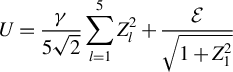
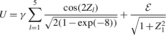

where $ \mathcal {E} \sim \mathcal {N}(0,1)$
independently of Z which follows the multivariate normal distribution with mean zero and covariance matrix
$ \mathcal {E} \sim \mathcal {N}(0,1)$
independently of Z which follows the multivariate normal distribution with mean zero and covariance matrix $\Sigma _{ll'} = 0.25^{|l-l'|}$
,
$\Sigma _{ll'} = 0.25^{|l-l'|}$
, ![]() , and
, and $\gamma \in [0,1]$
tunes the deviation away from
$\gamma \in [0,1]$
tunes the deviation away from $\mathbb {H}_o$
.
$\mathbb {H}_o$
. $X=Z$
in DGP LS1 and
$X=Z$
in DGP LS1 and $X_1 = (1.5Z_1 + \widetilde {\mathcal {E}}) / \sqrt {3.25} $
with
$X_1 = (1.5Z_1 + \widetilde {\mathcal {E}}) / \sqrt {3.25} $
with $\widetilde {\mathcal {E}}\sim \mathcal {N}(0,1)$
and
$\widetilde {\mathcal {E}}\sim \mathcal {N}(0,1)$
and $\mathrm {Cov}(\widetilde {\mathcal {E}},{\mathcal {E}})=0.25$
in DGPs LS2 through LS4.Footnote
8
Thus, X is exogenous under DGP LS1 and endogenous under DGPs LS2 through LS4. LS1 is estimated via ordinary least squares (OLS) while the remaining DGPs are estimated using the IVs estimator with Z as the instrument. Heteroskedasticity of arbitrary form is imposed in all DGPs.
$\mathrm {Cov}(\widetilde {\mathcal {E}},{\mathcal {E}})=0.25$
in DGPs LS2 through LS4.Footnote
8
Thus, X is exogenous under DGP LS1 and endogenous under DGPs LS2 through LS4. LS1 is estimated via ordinary least squares (OLS) while the remaining DGPs are estimated using the IVs estimator with Z as the instrument. Heteroskedasticity of arbitrary form is imposed in all DGPs.
Different sample sizes $n \in \{200, 400, 600, 800\}$
serve to examine the empirical size and local power of the test using DGPs LS1 and LS2 (with
$n \in \{200, 400, 600, 800\}$
serve to examine the empirical size and local power of the test using DGPs LS1 and LS2 (with $\gamma =0$
). For the analyses of power in DGPs LS2 through LS4, the sample size is kept at
$\gamma =0$
). For the analyses of power in DGPs LS2 through LS4, the sample size is kept at $n=400$
, while
$n=400$
, while $\gamma $
is varied in order to study the power of the proposed
$\gamma $
is varied in order to study the power of the proposed $\chi ^2$
-test in comparison to the bootstrap-based ICM procedures.
$\chi ^2$
-test in comparison to the bootstrap-based ICM procedures.
Empirical size and local power

4.2 Empirical Size and Power
Table 2 presents the empirical sizes corresponding to DGPs LS1 (under strictly exogenous X) and LS2 (under endogenous X instrumented with Z) in addition to the local power under LS2 at three nominal levels: 10%, 5%, and 1%. One observes comparably good size control of the proposed $\chi ^2$
-test and the bootstrap-based procedures across all the sample sizes considered. This provides evidence in support of the proposed test’s validity under both exogenous X and endogenous X with valid instruments Z.
$\chi ^2$
-test and the bootstrap-based procedures across all the sample sizes considered. This provides evidence in support of the proposed test’s validity under both exogenous X and endogenous X with valid instruments Z.
To ensure that the good size control of the $\chi ^2$
-test in Table 2 is not achieved at the expense of power under the alternative, we consider its performance under both local and fixed alternatives. The results, presented in the third panel of Table 2, indicate that the local power of the proposed
$\chi ^2$
-test in Table 2 is not achieved at the expense of power under the alternative, we consider its performance under both local and fixed alternatives. The results, presented in the third panel of Table 2, indicate that the local power of the proposed $\chi ^2$
-test, along with the bootstrap-based procedures, is non-trivial. Figures 1–6 present power curves corresponding to DGPs LS2 through LS4 using the Gaussian and Negative Euclidean kernels. One observes that all tests demonstrate non-trivial power against the fixed alternative for variations of
$\chi ^2$
-test, along with the bootstrap-based procedures, is non-trivial. Figures 1–6 present power curves corresponding to DGPs LS2 through LS4 using the Gaussian and Negative Euclidean kernels. One observes that all tests demonstrate non-trivial power against the fixed alternative for variations of $\gamma $
away from zero. The proposed test exhibits highly competitive power performance across all three DGPs and both kernels considered. Notably, the relative power of the
$\gamma $
away from zero. The proposed test exhibits highly competitive power performance across all three DGPs and both kernels considered. Notably, the relative power of the $\chi ^2$
-test compared to the bootstrap-based procedures demonstrates variability depending on the specific DGP and kernel, as highlighted in Theorem 3.3.
$\chi ^2$
-test compared to the bootstrap-based procedures demonstrates variability depending on the specific DGP and kernel, as highlighted in Theorem 3.3.
DGP LS2—Gaussian Kernel— $n=400$
.
$n=400$
.

DGP LS2—Negative Euclidean— $n=400$
.
$n=400$
.

DGP LS3—Gaussian Kernel— $n=400$
.
$n=400$
.

DGP LS3—Negative Euclidean— $n=400$
.
$n=400$
.

DGP LS4—Gaussian Kernel— $n=400$
.
$n=400$
.

DGP LS4—Negative Euclidean— $n=400$
.
$n=400$
.

Running time—specification test—DGP LS1

Note: The second row (in parentheses) for each sample size and kernel includes standard deviations and inter-quartile ranges for the average running times and relative times (the $\chi ^2$
-test as the benchmark), respectively.
$\chi ^2$
-test as the benchmark), respectively.
The $\chi ^2$
-test proves useful when researchers seek a measure of correct model specification or mean independence without resorting to a formal hypothesis test, owing to the pivotality of its test statistic. In summary, our simulations demonstrate that the proposed
$\chi ^2$
-test proves useful when researchers seek a measure of correct model specification or mean independence without resorting to a formal hypothesis test, owing to the pivotality of its test statistic. In summary, our simulations demonstrate that the proposed $\chi ^2$
-test, in addition to its enhanced interpretability compared to bootstrap-based ICM specification tests, exhibits good size control and comparable power performance.
$\chi ^2$
-test, in addition to its enhanced interpretability compared to bootstrap-based ICM specification tests, exhibits good size control and comparable power performance.
4.3 Running Time
One key advantage of a pivotal test is its computational efficiency relative to bootstrap-based procedures, which becomes particularly critical in large samples. Accordingly, a comparison of the running times of competing tests is in order. Table 3 presents a comparison between the proposed pivotal $\chi ^2$
-test and the bootstrap-based ICM tests in terms of computational time for fixed ICM kernels.Footnote
9
$\chi ^2$
-test and the bootstrap-based ICM tests in terms of computational time for fixed ICM kernels.Footnote
9
Table 3 illustrates the substantial computational advantage of employing the $\chi ^2$
specification test. The average running times for the
$\chi ^2$
specification test. The average running times for the $\chi ^2$
-test are negligible compared to those of the bootstrap-based procedures across all considered sample sizes. A striking difference emerges in terms of median relative computational time (with the
$\chi ^2$
-test are negligible compared to those of the bootstrap-based procedures across all considered sample sizes. A striking difference emerges in terms of median relative computational time (with the $\chi ^2$
-test serving as a benchmark). While the MB procedure is generally faster than the wild bootstrap procedure, our findings indicate that the median relative computational time of the MB tends to increase with the sample size, whereas that of the wild bootstrap appears to decrease. At particularly large sample sizes (
$\chi ^2$
-test serving as a benchmark). While the MB procedure is generally faster than the wild bootstrap procedure, our findings indicate that the median relative computational time of the MB tends to increase with the sample size, whereas that of the wild bootstrap appears to decrease. At particularly large sample sizes ( $n=600$
and
$n=600$
and $n=800$
), the computational gain offered by the
$n=800$
), the computational gain offered by the $\chi ^2$
-test becomes considerable.
$\chi ^2$
-test becomes considerable.
5 CONCLUSION
Despite the four-decade history of ICM tests, dating back to Bierens (Reference Bierens1982) and encompassing numerous interesting contributions, a bona fide pivotalized ICM specification test remains lacking. This article achieves the objective of proposing an omnibus $\chi ^2$
-test of specification and mean independence based on ICM metrics.
$\chi ^2$
-test of specification and mean independence based on ICM metrics.
The proposed $\chi ^2$
-test complements existing ICM tests by overcoming certain limitations of the latter. The test statistic can be constructed with functional forms that boost power in the direction of alternatives the researcher may have in mind. The test is computationally more efficient than commonly used bootstrap-based ICM tests and remains computationally viable even in large samples. In addition to providing a reliable pivotal test that derives its omnibus property from ICM metrics, the test statistic offers an easily interpretable metric of model specification and mean dependence, thereby obviating formal hypothesis tests.
$\chi ^2$
-test complements existing ICM tests by overcoming certain limitations of the latter. The test statistic can be constructed with functional forms that boost power in the direction of alternatives the researcher may have in mind. The test is computationally more efficient than commonly used bootstrap-based ICM tests and remains computationally viable even in large samples. In addition to providing a reliable pivotal test that derives its omnibus property from ICM metrics, the test statistic offers an easily interpretable metric of model specification and mean dependence, thereby obviating formal hypothesis tests.
In conclusion, we highlight several potential extensions to the current work. While this article offers a viable solution for pivotalizing ICM tests, it is noteworthy that this approach necessitates regularization under the null hypothesis to address the ill-posed inverse problem. Future research could explore alternative formulations of V that may yield solutions with more desirable theoretical properties. Furthermore, extending our analysis from the current fixed-dimensional setting to a high-dimensional framework presents an interesting avenue for research. Moreover, leveraging the projection approach proposed by Escanciano (Reference Escanciano2009b, Reference Escanciano2024), which eliminates the estimation effect, could be advantageous in dealing with estimators whose limiting distributions are difficult to characterize, for example, the LASSO. Finally, extending our methodology to encompass time series data, clustered data, and multiple-equation models with (non)-smooth objective functions warrants future exploration.
COMPETING INTEREST STATEMENT
The authors declare that no competing interests exist.
FUNDING STATEMENT
F.J.’s research is supported in part by the National Key R&D Program of China (Grant No. 2024YFA1015700) and by the NSFC (Grant Nos. 72522009, 12201124, 12331009, 72271060, and 72432002).
SUPPLEMENTARY MATERIAL
Proofs of all results and additional numerical results are provided in Jiang and Tsyawo (2025): Supplement to “A Consistent ICM-Based $\chi ^2$
Specification Test,” Econometric Theory Supplementary Material. To view, please visit: https://doi.org/10.1017/S0266466626100437.
$\chi ^2$
Specification Test,” Econometric Theory Supplementary Material. To view, please visit: https://doi.org/10.1017/S0266466626100437.


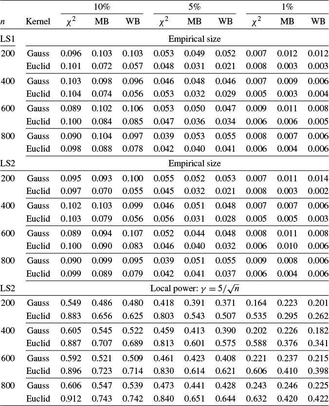


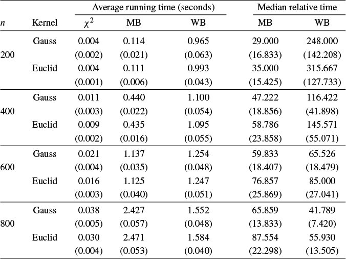


 Open access