





1. Introduction
Millisecond pulsars (MSPs) are extremely valuable astrophysical tools due to the precision with which their pulses can be timed in both radio and gamma-rays (e.g. arrival time estimates with $\mathbin{\sim}\unicode{x03BC}\mathrm{s}$
uncertainties; Spiewak et al. Reference Spiewak2022; Valtolina et al. Reference Valtolina, Clark, van Haasteren, Chalumeau, Cromartie, Kerr, Nieder and Parthasarathy2026). Around one in five of the over 600 Galactic MSPsFootnote
a
discovered to date have been found in targeted radio searches of unassociated gamma-ray sources detected by the Large Area Telescope (LAT) onboard Fermi (Ray et al. Reference Ray2012). Almost all of these surveys have been conducted at radio frequencies above
$\mathbin{\sim}\unicode{x03BC}\mathrm{s}$
uncertainties; Spiewak et al. Reference Spiewak2022; Valtolina et al. Reference Valtolina, Clark, van Haasteren, Chalumeau, Cromartie, Kerr, Nieder and Parthasarathy2026). Around one in five of the over 600 Galactic MSPsFootnote
a
discovered to date have been found in targeted radio searches of unassociated gamma-ray sources detected by the Large Area Telescope (LAT) onboard Fermi (Ray et al. Reference Ray2012). Almost all of these surveys have been conducted at radio frequencies above $300\,\mathrm{MHz}$
; either at
$300\,\mathrm{MHz}$
; either at $1.4\,\mathrm{GHz}$
(e.g. Cognard et al. Reference Cognard2011; Barr et al. Reference Barr2013; Camilo et al. Reference Camilo2015; Clark et al. Reference Clark2023),
$1.4\,\mathrm{GHz}$
(e.g. Cognard et al. Reference Cognard2011; Barr et al. Reference Barr2013; Camilo et al. Reference Camilo2015; Clark et al. Reference Clark2023), $820\,\mathrm{MHz}$
(e.g. Ransom et al. Reference Ransom2011; Thongmeearkom et al. Reference Thongmeearkom2026), or
$820\,\mathrm{MHz}$
(e.g. Ransom et al. Reference Ransom2011; Thongmeearkom et al. Reference Thongmeearkom2026), or $350\,\mathrm{MHz}$
(e.g. Hessels et al. Reference Hessels, Burgay, D’Amico, Esposito, Pellizzoni and Possenti2011; Cromartie et al. Reference Cromartie2016; Bangale et al. Reference Bangale2024). These surveys have been particularly effective in discovering ‘spider’ systems, which consist of a pulsar in a compact binary with a low-mass companion, often exhibiting radio eclipses. Spider pulsars can be used to study binary pulsar evolution, particle acceleration, and measure neutron star masses (see Koljonen & Linares Reference Koljonen and Linares2025, for a summary). Furthermore, 25 MSPs discovered in Fermi-guided radio searches have since been included in pulsar timing arrays (PTAs), increasing the sensitivity to low-frequency gravitational waves (e.g. Siemens et al. Reference Siemens, Ellis, Jenet and Romano2013). The fourth Fermi-LAT source catalogue (4FGL; Abdollahi et al. Reference Abdollahi2020) contains 1 336 unassociated gamma-ray sources, many of which are likely to be pulsars. A recent population synthesis by Sautron et al. (Reference Sautron, Pétri, Mitra, Dupuy-Junet and Pietrin2026) predicted that there remain up to 220 unidentified pulsars to be discovered in the 4FGL catalogue. There is also evidence suggesting that the fastest MSPs tend to be detected in gamma-rays and have unusually steep radio spectra (e.g. Espinoza et al. Reference Espinoza2013; Bassa et al. Reference Bassa, Pleunis and Hessels2017). There is, therefore, ample motivation to continue searching these sources, particularly at frequencies below
$350\,\mathrm{MHz}$
(e.g. Hessels et al. Reference Hessels, Burgay, D’Amico, Esposito, Pellizzoni and Possenti2011; Cromartie et al. Reference Cromartie2016; Bangale et al. Reference Bangale2024). These surveys have been particularly effective in discovering ‘spider’ systems, which consist of a pulsar in a compact binary with a low-mass companion, often exhibiting radio eclipses. Spider pulsars can be used to study binary pulsar evolution, particle acceleration, and measure neutron star masses (see Koljonen & Linares Reference Koljonen and Linares2025, for a summary). Furthermore, 25 MSPs discovered in Fermi-guided radio searches have since been included in pulsar timing arrays (PTAs), increasing the sensitivity to low-frequency gravitational waves (e.g. Siemens et al. Reference Siemens, Ellis, Jenet and Romano2013). The fourth Fermi-LAT source catalogue (4FGL; Abdollahi et al. Reference Abdollahi2020) contains 1 336 unassociated gamma-ray sources, many of which are likely to be pulsars. A recent population synthesis by Sautron et al. (Reference Sautron, Pétri, Mitra, Dupuy-Junet and Pietrin2026) predicted that there remain up to 220 unidentified pulsars to be discovered in the 4FGL catalogue. There is also evidence suggesting that the fastest MSPs tend to be detected in gamma-rays and have unusually steep radio spectra (e.g. Espinoza et al. Reference Espinoza2013; Bassa et al. Reference Bassa, Pleunis and Hessels2017). There is, therefore, ample motivation to continue searching these sources, particularly at frequencies below $300\,\mathrm{MHz}$
and above
$300\,\mathrm{MHz}$
and above $2\,\mathrm{GHz}$
where fewer surveys have been performed and there may be detectable pulsars with steeper or shallower intrinsic flux density spectra.
$2\,\mathrm{GHz}$
where fewer surveys have been performed and there may be detectable pulsars with steeper or shallower intrinsic flux density spectra.
Surveys below $300\,\mathrm{MHz}$
face several challenges due to chromatic effects on the radio signals imparted by the cold ionised interstellar medium (IISM). Perhaps the most significant challenge is the computational cost of correcting the large dispersive delays over the receiver bandwidth. Pulses propagating through the IISM experience a delay proportional to
$300\,\mathrm{MHz}$
face several challenges due to chromatic effects on the radio signals imparted by the cold ionised interstellar medium (IISM). Perhaps the most significant challenge is the computational cost of correcting the large dispersive delays over the receiver bandwidth. Pulses propagating through the IISM experience a delay proportional to $\nu^{-2}$
(where
$\nu^{-2}$
(where $\nu$
is the observational frequency) and the dispersion measure (DM), which represents the column density of free electrons along the path of propagation (see Section 4.1.1 of Lorimer & Kramer Reference Lorimer and Kramer2012). As a result, pulses arrive at the receiver later at lower frequencies than their higher frequency counterparts, causing temporal smearing in the recorded time series. Pulsar surveys must search over a range of DMs to identify dispersed signals. Dispersion can be partially corrected by channelising the received signal and applying the appropriate time delays so that each pulse arrives simultaneously in all channels (i.e. ‘incoherent’ dedispersion). However, without correcting the dispersion within the frequency channels (intrachannel dispersion), there will always be residual dispersive smearing. This is a particularly significant issue when searching for short-period pulsars at low frequencies, where intrachannel dispersive smearing can limit searches to very low DMs. Assuming the intervening medium is a cold tenuous plasma (as is the case for the IISM), intrachannel dispersion can be completely removed by phase-coherently dedispersing the complex voltages for each channel (Hankins Reference Hankins1971; van Straten & Bailes Reference van Straten and Bailes2011). However, this requires several computationally expensive steps that make fully-coherent searches largely impractical. Bassa et al. (Reference Bassa, Pleunis and Hessels2017) proposed an alternative ‘semi-coherent’ dedispersion strategy, which involves performing phase-coherent dedispersion to a smaller number of DMs (e.g.
$\nu$
is the observational frequency) and the dispersion measure (DM), which represents the column density of free electrons along the path of propagation (see Section 4.1.1 of Lorimer & Kramer Reference Lorimer and Kramer2012). As a result, pulses arrive at the receiver later at lower frequencies than their higher frequency counterparts, causing temporal smearing in the recorded time series. Pulsar surveys must search over a range of DMs to identify dispersed signals. Dispersion can be partially corrected by channelising the received signal and applying the appropriate time delays so that each pulse arrives simultaneously in all channels (i.e. ‘incoherent’ dedispersion). However, without correcting the dispersion within the frequency channels (intrachannel dispersion), there will always be residual dispersive smearing. This is a particularly significant issue when searching for short-period pulsars at low frequencies, where intrachannel dispersive smearing can limit searches to very low DMs. Assuming the intervening medium is a cold tenuous plasma (as is the case for the IISM), intrachannel dispersion can be completely removed by phase-coherently dedispersing the complex voltages for each channel (Hankins Reference Hankins1971; van Straten & Bailes Reference van Straten and Bailes2011). However, this requires several computationally expensive steps that make fully-coherent searches largely impractical. Bassa et al. (Reference Bassa, Pleunis and Hessels2017) proposed an alternative ‘semi-coherent’ dedispersion strategy, which involves performing phase-coherent dedispersion to a smaller number of DMs (e.g. $\Delta\mathrm{DM}\sim 1\,\mathrm{cm}^{-3}\,{\rm pc}$
), then incoherently dedispersing to a larger number of DMs in between each coherent step (e.g.
$\Delta\mathrm{DM}\sim 1\,\mathrm{cm}^{-3}\,{\rm pc}$
), then incoherently dedispersing to a larger number of DMs in between each coherent step (e.g. $\Delta\mathrm{DM}\sim 10^{-3}\,\mathrm{cm}^{-3}\,\mathrm{pc}$
). By carefully choosing the DM step sizes, one can effectively trade off between computational cost and dispersive smearing. This novel approach was used to discover three MSPs in a targeted survey of unassociated Fermi-LAT sources with the Low-Frequency Array (LOFAR) at
$\Delta\mathrm{DM}\sim 10^{-3}\,\mathrm{cm}^{-3}\,\mathrm{pc}$
). By carefully choosing the DM step sizes, one can effectively trade off between computational cost and dispersive smearing. This novel approach was used to discover three MSPs in a targeted survey of unassociated Fermi-LAT sources with the Low-Frequency Array (LOFAR) at $135\,\mathrm{MHz}$
(Pleunis et al. Reference Pleunis2017; Bassa et al. Reference Bassa, Pleunis and Hessels2017; Bassa et al. Reference Bassa, Weltevrede, Perera, Preston and Sanidas2018).
$135\,\mathrm{MHz}$
(Pleunis et al. Reference Pleunis2017; Bassa et al. Reference Bassa, Pleunis and Hessels2017; Bassa et al. Reference Bassa, Weltevrede, Perera, Preston and Sanidas2018).
The demonstrated benefits of semi-coherent dedispersion in the LOFAR survey motivated us to apply the technique to pulsar searches with the Murchison Widefield Array (MWA). The MWA is a low-frequency aperture array telescope located at Inyarrimanha Ilgari Bundara, the CSIRO Murchison Radio-astronomy Observatory in Western Australia (Tingay et al. Reference Tingay2013). It operates between $70\text{--}300\,\mathrm{MHz}$
and can observe declinations south of around
$70\text{--}300\,\mathrm{MHz}$
and can observe declinations south of around $+30^\circ$
. It is currently the most sensitive telescope operating below 300 MHz with access to the entire southern sky. The MWA’s Voltage Capture System (VCS; Tremblay et al. Reference Tremblay2015; Morrison et al. Reference Morrison2023) provides the capability to record the complex voltages from each of the tiles in the array (
$+30^\circ$
. It is currently the most sensitive telescope operating below 300 MHz with access to the entire southern sky. The MWA’s Voltage Capture System (VCS; Tremblay et al. Reference Tremblay2015; Morrison et al. Reference Morrison2023) provides the capability to record the complex voltages from each of the tiles in the array ( $\sim$
128 tiles in Phase II; Wayth et al. Reference Wayth2018) over a
$\sim$
128 tiles in Phase II; Wayth et al. Reference Wayth2018) over a $30.72\,\mathrm{MHz}$
observing bandwidth. To exploit the flexibility of VCS data, the Southern-sky MWA Rapid Two-metre (SMART) pulsar survey was conceived, comprising 71 drift-scan observations that together cover the entire sky within the declination range of the telescope with a dwell time of
$30.72\,\mathrm{MHz}$
observing bandwidth. To exploit the flexibility of VCS data, the Southern-sky MWA Rapid Two-metre (SMART) pulsar survey was conceived, comprising 71 drift-scan observations that together cover the entire sky within the declination range of the telescope with a dwell time of $80\,\mathrm{min}$
(Bhat et al. Reference Bhat2023a,Reference Bhatb). The primary objective of SMART is to conduct an untargeted all-sky survey for pulsars. However, the dispersive smearing limits detections to
$80\,\mathrm{min}$
(Bhat et al. Reference Bhat2023a,Reference Bhatb). The primary objective of SMART is to conduct an untargeted all-sky survey for pulsars. However, the dispersive smearing limits detections to $\mathrm{DM}\lesssim30\,\mathrm{cm}^{-3}\,{\rm pc}$
for MSPs (Bhat et al. Reference Bhat2023a). Given the high computational cost of processing and searching through the SMART data set, it is also infeasible to perform orbital acceleration searches for the full survey. This means that the survey is not sensitive to pulsars in short-orbit binaries, including the majority of MSPs that have been discovered in Fermi-guided radio searches.
$\mathrm{DM}\lesssim30\,\mathrm{cm}^{-3}\,{\rm pc}$
for MSPs (Bhat et al. Reference Bhat2023a). Given the high computational cost of processing and searching through the SMART data set, it is also infeasible to perform orbital acceleration searches for the full survey. This means that the survey is not sensitive to pulsars in short-orbit binaries, including the majority of MSPs that have been discovered in Fermi-guided radio searches.
To improve sensitivity to MSPs and exploit the unexplored period/DM/acceleration parameter space in the SMART survey, we have developed a semi-coherent dedispersion pipeline intended for targeted MSP searches in MWA data. These searches will complement LOFAR by targeting Fermi-LAT sources in the southern hemisphere below $300\,\mathrm{MHz}$
for the first time. In Section 2, we describe the pipeline workflow and implementation and validate it by blindly detecting known MSPs. In Section 3, we describe a pilot survey of unassociated Fermi-LAT sources in the SMART data, including the target selection, sensitivity, and search results. In Section 4, we discuss the limitations of the survey and the prospects for discovering MSPs with the MWA Phase III. Lastly, in Section 5, we conclude and provide recommendations for future targeted searches with the MWA.
$300\,\mathrm{MHz}$
for the first time. In Section 2, we describe the pipeline workflow and implementation and validate it by blindly detecting known MSPs. In Section 3, we describe a pilot survey of unassociated Fermi-LAT sources in the SMART data, including the target selection, sensitivity, and search results. In Section 4, we discuss the limitations of the survey and the prospects for discovering MSPs with the MWA Phase III. Lastly, in Section 5, we conclude and provide recommendations for future targeted searches with the MWA.
2. Search pipeline
2.1. Description
The MWA tile voltages recorded by the VCS are coherently combined into a tied-array beam using the GPU-accelerated beamforming software vcsbeam (Ord et al. Reference Ord, Tremblay, McSweeney, Bhat, Sobey, Mitchell, Hancock and Kirsten2019; Bhat et al. Reference Bhat2026). The beamformed data are stored as 8+8-bit complex samples in the VLBI Data Interchange Format (VDIF)Footnote
b
with one data file and one header file for each of the $24\times1.28\,\mathrm{MHz}$
coarse channels (i.e. receiver channels), with a native time resolution of
$24\times1.28\,\mathrm{MHz}$
coarse channels (i.e. receiver channels), with a native time resolution of $781.25\,\mathrm{ns}$
. The VDIF data, along with a dedispersion plan, are provided as inputs to the search pipeline. The pipeline workflow is summarised in Figure 1.
$781.25\,\mathrm{ns}$
. The VDIF data, along with a dedispersion plan, are provided as inputs to the search pipeline. The pipeline workflow is summarised in Figure 1.
Diagram illustrating the basic workflow of the semi-coherent pulsar search pipeline. Red rounded boxes indicate GPU-based processing tasks and blue rounded boxes indicate CPU-based processing tasks. See Sections 2.1 and 2.2 for details.

Figure 1. Long description
A diagram illustrating the workflow of the semi-coherent pulsar search pipeline. The diagram shows a series of processes and tasks involved in the pipeline, with red rounded boxes indicating GPU-based processing tasks and blue rounded boxes indicating CPU-based processing tasks. The workflow begins with a tied-array voltage beam in VDIF format. The beam is coherently dedispersed, channelised, and detected using CDMT, producing a SIGPROC filterbank. The filterbank is cleaned with IQRM channel flagging. Next, the filterbank is incoherently dedispersed using Fourier-domain dedispersion, producing time series with 50-microsecond resolution. The time series are searched with a Fourier-domain acceleration search, then the candidates are sifted with ACCEL_sift.py, and the sifted candidates are folded with prepfold. An RFI mask is applied that is created by RFIFIND. The end products are candidate plots and the folded detection significance.
We perform the phase-coherent dedispersion using cdmt – a GPU-accelerated software designed to efficiently dedisperse to multiple DMs using a convolving filterbank (Bassa et al. Reference Bassa2017). cdmt also performs channelisation and detection into Stokes I. As the code was originally designed to read LOFAR data in HDF5 format, we have modified it to read VDIF data.Footnote
c
The detected data for each coherent DM trial are stored as 8-bit sigproc filterbanks (Lorimer Reference Lorimer2011) containing $1\,536\times20\,\mathrm{kHz}$
channels with a time resolution of
$1\,536\times20\,\mathrm{kHz}$
channels with a time resolution of $50\,\unicode{x03BC}s$
. Each filterbank is then incoherently dedispersed using the GPU-accelerated Fourier domain dedispersion (FDD) algorithm implemented by Bassa et al. (Reference Bassa, Romein, Veenboer, van der Vlugt and Wijnholds2022) in a fork of the dedisp library.Footnote
d
The dedispersed time series for each DM trial are stored as 32-bit floats in a binary file with an accompanying header file for compatibility with presto (Ransom Reference Ransom2001).
$50\,\unicode{x03BC}s$
. Each filterbank is then incoherently dedispersed using the GPU-accelerated Fourier domain dedispersion (FDD) algorithm implemented by Bassa et al. (Reference Bassa, Romein, Veenboer, van der Vlugt and Wijnholds2022) in a fork of the dedisp library.Footnote
d
The dedispersed time series for each DM trial are stored as 32-bit floats in a binary file with an accompanying header file for compatibility with presto (Ransom Reference Ransom2001).
We search for the signals of binary pulsars in the dedispersed time series using the accelsearch routine from presto, which implements the Fourier-domain acceleration search (FDAS) to identify pulsar candidates. The FDAS is described in detail in Ransom et al. (Reference Ransom, Eikenberry and Middleditch2002), and a summary is provided in Andersen & Ransom (Reference Andersen and Ransom2018). For the FDAS, we assume that the observation length $T$
is a sufficiently small fraction of the binary orbital period
$T$
is a sufficiently small fraction of the binary orbital period $P_{\mathrm{orb}}$
, such that the orbital acceleration of the pulsar can be approximated as constant. Each harmonic of the fundamental spin frequency
$P_{\mathrm{orb}}$
, such that the orbital acceleration of the pulsar can be approximated as constant. Each harmonic of the fundamental spin frequency $f_0$
would then exhibit a constant frequency derivative
$f_0$
would then exhibit a constant frequency derivative $\dot{f}$
, causing the signal to drift through
$\dot{f}$
, causing the signal to drift through $z=\dot{f}T^2$
bins in each Fourier power spectrum (where z is the Fourier frequency derivative). In this case, the acceleration may be expressed as
$z=\dot{f}T^2$
bins in each Fourier power spectrum (where z is the Fourier frequency derivative). In this case, the acceleration may be expressed as
 \begin{equation} \alpha = \frac{\dot{f}c}{hf_0}= \frac{zc}{hf_0T^2},\end{equation}
where c is the speed of light and h is the harmonic number ( $h=1$
is the fundamental). The FDAS involves generating a set of template filters for a range of trial values of
$h=1$
is the fundamental). The FDAS involves generating a set of template filters for a range of trial values of $\dot{f}$
, and correlating the templates with the complex-valued Fourier-transformed time series. The Fourier components are converted to powers and normalised by a block running median, which removes red noise and allows for accurate estimation of signal significances. The Fourier power spectra for the
$\dot{f}$
, and correlating the templates with the complex-valued Fourier-transformed time series. The Fourier components are converted to powers and normalised by a block running median, which removes red noise and allows for accurate estimation of signal significances. The Fourier power spectra for the $\dot{f}$
trials are then combined to form a 2D plane of powers in
$\dot{f}$
trials are then combined to form a 2D plane of powers in $f-\dot{f}$
space. Candidate signals are identified via threshold searching in the
$f-\dot{f}$
space. Candidate signals are identified via threshold searching in the $f-\dot{f}$
plane and incoherently summing harmonics to increase the sensitivity. As discussed in Andersen & Ransom (Reference Andersen and Ransom2018), most MSPs with stellar-mass companions are detectable with
$f-\dot{f}$
plane and incoherently summing harmonics to increase the sensitivity. As discussed in Andersen & Ransom (Reference Andersen and Ransom2018), most MSPs with stellar-mass companions are detectable with $|z|\lt 200$
if
$|z|\lt 200$
if $T\lesssim0.1P_{\mathrm{orb}}$
. We search z values from
$T\lesssim0.1P_{\mathrm{orb}}$
. We search z values from $-200$
to 200 in steps of
$-200$
to 200 in steps of $\Delta z=2$
(i.e. 201 acceleration trials), and spin frequencies from
$\Delta z=2$
(i.e. 201 acceleration trials), and spin frequencies from $0.5\,\mathrm{Hz}$
to
$0.5\,\mathrm{Hz}$
to $10\,\mathrm{kHz}$
with up to
$10\,\mathrm{kHz}$
with up to $N_{\mathrm{harm}}=8$
summed harmonics. We are therefore sensitive to the 8th harmonic of signals with
$N_{\mathrm{harm}}=8$
summed harmonics. We are therefore sensitive to the 8th harmonic of signals with $f_0\lt 1.25\,\mathrm{kHz}$
(or
$f_0\lt 1.25\,\mathrm{kHz}$
(or $P\gt 0.8\,\mathrm{ms}$
). To compare candidates over multiple DM trials, accelsearch calculates the probability that the summed harmonic power of a candidate is due to noise (corrected for the number of independent f and
$P\gt 0.8\,\mathrm{ms}$
). To compare candidates over multiple DM trials, accelsearch calculates the probability that the summed harmonic power of a candidate is due to noise (corrected for the number of independent f and $\dot{f}$
trials searched), and expresses it in terms of its equivalent Gaussian significance,
$\dot{f}$
trials searched), and expresses it in terms of its equivalent Gaussian significance, $\sigma_{\mathrm{FFT}}$
.
$\sigma_{\mathrm{FFT}}$
.
The accelsearch candidates for all of the DM trials are then grouped and sifted using python utilities provided by presto. First, candidates are rejected if (1) $\sigma_{\mathrm{FFT}}\lt 6$
; (2) the candidate is detected in only 1 harmonic that has a normalised Fourier power less than 100; (3) the candidate is detected in multiple harmonics, but all harmonics have a normalised Fourier power less than 3; or (4) the candidate is dominated by a single high-power and high-order harmonic. The candidates are then grouped by period and DM, and are rejected if they appear in less than 5 DM trials or if the best DM is less than
$\sigma_{\mathrm{FFT}}\lt 6$
; (2) the candidate is detected in only 1 harmonic that has a normalised Fourier power less than 100; (3) the candidate is detected in multiple harmonics, but all harmonics have a normalised Fourier power less than 3; or (4) the candidate is dominated by a single high-power and high-order harmonic. The candidates are then grouped by period and DM, and are rejected if they appear in less than 5 DM trials or if the best DM is less than $1\,\mathrm{cm}^{-3}\,\mathrm{pc}$
. Only the candidate from the DM with the highest
$1\,\mathrm{cm}^{-3}\,\mathrm{pc}$
. Only the candidate from the DM with the highest $\sigma_{\mathrm{FFT}}$
is kept. Finally, harmonically related candidates are grouped and only the harmonic with the highest
$\sigma_{\mathrm{FFT}}$
is kept. Finally, harmonically related candidates are grouped and only the harmonic with the highest $\sigma_{\mathrm{FFT}}$
is kept. The candidate list is then sorted by
$\sigma_{\mathrm{FFT}}$
is kept. The candidate list is then sorted by $\sigma_{\mathrm{FFT}}$
. For our searches,
$\sigma_{\mathrm{FFT}}$
. For our searches, $\sim$
100 candidates typically remain per pointing after sifting. Although the candidates with
$\sim$
100 candidates typically remain per pointing after sifting. Although the candidates with $\sigma_{\mathrm{FFT}}$
between 6 and 10 are mostly due to noise, pulsars with narrow duty cycles will often experience a ‘boost’ in significance when folded and optimised, due to the limited number of harmonics summed in the FDAS (Sengar et al. Reference Sengar2023). Since our searches are targeted, we can afford to fold candidates down to a lower
$\sigma_{\mathrm{FFT}}$
between 6 and 10 are mostly due to noise, pulsars with narrow duty cycles will often experience a ‘boost’ in significance when folded and optimised, due to the limited number of harmonics summed in the FDAS (Sengar et al. Reference Sengar2023). Since our searches are targeted, we can afford to fold candidates down to a lower $\sigma_{\mathrm{FFT}}$
to take advantage of this effect.
$\sigma_{\mathrm{FFT}}$
to take advantage of this effect.
We then use the prepfold routine from presto to dedisperse and fold the filterbank data at the DM, f, and $\dot{f}$
of each candidate with 10-s subintegrations, 240-kHz subbands, and 64 phase bins. prepfold determines the optimal values for the DM, f, and
$\dot{f}$
of each candidate with 10-s subintegrations, 240-kHz subbands, and 64 phase bins. prepfold determines the optimal values for the DM, f, and $\dot{f}$
by performing a fine grid search around the candidate values and maximising the reduced
$\dot{f}$
by performing a fine grid search around the candidate values and maximising the reduced $\chi^2$
of the profile. A candidate plot is then generated displaying the folded data and other diagnostics to aid with interpretation. Similar to accelsearch, prepfold also estimates the probability that the pulsations are due to noise and expresses it in terms of its equivalent Gaussian significance,
$\chi^2$
of the profile. A candidate plot is then generated displaying the folded data and other diagnostics to aid with interpretation. Similar to accelsearch, prepfold also estimates the probability that the pulsations are due to noise and expresses it in terms of its equivalent Gaussian significance, $\sigma_{\mathrm{fold}}$
.
$\sigma_{\mathrm{fold}}$
.
Although the SMART survey data are generally exceptionally clean, it is still necessary to perform basic mitigation of radio frequency interference (RFI). To reduce spurious accelsearch candidates caused by strong and persistent narrowband RFI, outlier frequency channels in the sigproc filterbanks are flagged using Inter-Quartile Range Mitigation (IQRM; Morello et al. Reference Morello, Rajwade and Stappers2022) with a threshold of $4\sigma$
and a radius of 5 channels (
$4\sigma$
and a radius of 5 channels ( $100\,\mathrm{kHz}$
). We use the implementation of IQRM in the spp_clean utility provided by sigpyproc3.Footnote
e
Additionally, we create an RFI mask for each filterbank using the rfifind routine from presto. We use time blocks of
$100\,\mathrm{kHz}$
). We use the implementation of IQRM in the spp_clean utility provided by sigpyproc3.Footnote
e
Additionally, we create an RFI mask for each filterbank using the rfifind routine from presto. We use time blocks of $16\,\mathrm{s}$
and explicitly mask 4 channels (
$16\,\mathrm{s}$
and explicitly mask 4 channels ( $80\,\mathrm{kHz}$
) at the top and bottom edges of each coarse channel (i.e. 12.5% of the bandwidth). The rfifind masks are applied by prepfold before folding, which reduces both impulsive broadband RFI and weaker narrowband RFI in the folded data. prepfold also performs clipping of outlier samples at zero DM; however, because the filterbanks are phase-coherently dedispersed, signals at zero DM will be subject to intrachannel dispersive smearing, making impulsive RFI less significant.
$80\,\mathrm{kHz}$
) at the top and bottom edges of each coarse channel (i.e. 12.5% of the bandwidth). The rfifind masks are applied by prepfold before folding, which reduces both impulsive broadband RFI and weaker narrowband RFI in the folded data. prepfold also performs clipping of outlier samples at zero DM; however, because the filterbanks are phase-coherently dedispersed, signals at zero DM will be subject to intrachannel dispersive smearing, making impulsive RFI less significant.
The ranked list of candidates, candidate plots, and rfifind results (which includes summary plots and statistics) are saved for each search. The candidate plots are inspected by eye for persistent broadband pulsations and peaks in the reduced $\chi^2$
as a function of DM, spin period (P), and spin period derivative (
$\chi^2$
as a function of DM, spin period (P), and spin period derivative ( $\dot{P}$
), which are all features of real pulsar signals. Candidates are generally rejected if the signal is impulsive or narrowband, has a DM close to zero, or has a spin period that is a harmonic of a known terrestrial signal. In some cases, the rfifind results are used as a diagnostic to assess the presence of RFI in the data.
$\dot{P}$
), which are all features of real pulsar signals. Candidates are generally rejected if the signal is impulsive or narrowband, has a DM close to zero, or has a spin period that is a harmonic of a known terrestrial signal. In some cases, the rfifind results are used as a diagnostic to assess the presence of RFI in the data.
2.2. Dedispersion plan
The temporal smearing ( $\tau_{\mathrm{smear}}$
) of a search is the sum in quadrature of the sample time (
$\tau_{\mathrm{smear}}$
) of a search is the sum in quadrature of the sample time ( $\delta t$
), the intrachannel dispersive smearingFootnote
f
(
$\delta t$
), the intrachannel dispersive smearingFootnote
f
( $\tau_{\mathrm{DM}}$
), and the dispersive smearing due to the difference between the DM of the pulsar and the nearest trial DM (
$\tau_{\mathrm{DM}}$
), and the dispersive smearing due to the difference between the DM of the pulsar and the nearest trial DM ( $\tau_{\delta\mathrm{DM}}$
):
$\tau_{\delta\mathrm{DM}}$
):
 \begin{equation} \tau_{\mathrm{smear}} = \sqrt{\delta t^2 + \tau_{\mathrm{DM}}^2 + \tau_{\delta\mathrm{DM}}^2}.\end{equation}
We have chosen a semi-coherent dedispersion plan that limits the temporal smearing to $136.1\,\unicode{x03BC}s$
in the SMART frequency band for frequency/time resolutions of
$136.1\,\unicode{x03BC}s$
in the SMART frequency band for frequency/time resolutions of $20\,\mathrm{kHz}$
/
$20\,\mathrm{kHz}$
/ $50\,\unicode{x03BC}s$
. The data are first phase-coherently dedispersed to 27 DMs from 1.5 to
$50\,\unicode{x03BC}s$
. The data are first phase-coherently dedispersed to 27 DMs from 1.5 to $79.5 \,\mathrm{cm}^{-3}\,\mathrm{pc}$
in steps of
$79.5 \,\mathrm{cm}^{-3}\,\mathrm{pc}$
in steps of $3 \,\mathrm{cm}^{-3}\,\mathrm{pc}$
. They are then incoherently dedispersed to
$3 \,\mathrm{cm}^{-3}\,\mathrm{pc}$
. They are then incoherently dedispersed to $\pm 1.5 \,\mathrm{cm}^{-3}\,\mathrm{pc}$
in steps of
$\pm 1.5 \,\mathrm{cm}^{-3}\,\mathrm{pc}$
in steps of $0.003 \,\mathrm{cm}^{-3}\,\mathrm{pc}$
around each coherent DM. This results in a total of 27 000 DM trials. The worst-case smearing (i.e. when
$0.003 \,\mathrm{cm}^{-3}\,\mathrm{pc}$
around each coherent DM. This results in a total of 27 000 DM trials. The worst-case smearing (i.e. when $\tau_{\delta\mathrm{DM}}$
is maximised) for the semi-coherent dedispersion plan is shown as a function of DM in Figure 2, along with a fully incoherent dedispersion plan and the untargeted SMART survey dedispersion plan for comparison. We also show how the minimum detectable flux density scales with DM for a typical MSP, with and without pulse broadening due to scattering (see Section 3.2 for details on the sensitivity calculations).
$\tau_{\delta\mathrm{DM}}$
is maximised) for the semi-coherent dedispersion plan is shown as a function of DM in Figure 2, along with a fully incoherent dedispersion plan and the untargeted SMART survey dedispersion plan for comparison. We also show how the minimum detectable flux density scales with DM for a typical MSP, with and without pulse broadening due to scattering (see Section 3.2 for details on the sensitivity calculations).
Comparison of dedispersion plans in the SMART frequency band ( $138.88\text{--}169.60\,\mathrm{MHz}$
). Top: The worst-case temporal smearing (i.e.
$138.88\text{--}169.60\,\mathrm{MHz}$
). Top: The worst-case temporal smearing (i.e. $\tau_{\mathrm{smear}}$
assuming the maximum
$\tau_{\mathrm{smear}}$
assuming the maximum $\tau_{\delta\mathrm{DM}}$
) as a function of DM. The estimated scattering time (
$\tau_{\delta\mathrm{DM}}$
) as a function of DM. The estimated scattering time ( $\tau_{\mathrm{scatt}}$
) is shown with an order-of-magnitude error band (Bhat et al. Reference Bhat, Cordes, Camilo, Nice and Lorimer2004). The test pulsars are indicated at their respective spin periods and DMs and labelled by their right ascension. Bottom: The minimum detectable flux density (
$\tau_{\mathrm{scatt}}$
) is shown with an order-of-magnitude error band (Bhat et al. Reference Bhat, Cordes, Camilo, Nice and Lorimer2004). The test pulsars are indicated at their respective spin periods and DMs and labelled by their right ascension. Bottom: The minimum detectable flux density ( $S_{\mathrm{min}}$
) for a pulsar with a spin period of
$S_{\mathrm{min}}$
) for a pulsar with a spin period of $2\,\mathrm{ms}$
and a duty cycle of 28%, assuming an integration time of
$2\,\mathrm{ms}$
and a duty cycle of 28%, assuming an integration time of $20\,\mathrm{min}$
and a SEFD of
$20\,\mathrm{min}$
and a SEFD of $1\,\mathrm{kJy}$
(i.e. MWA Phase II sensitivity away from the Galactic plane). The grey and black lines show
$1\,\mathrm{kJy}$
(i.e. MWA Phase II sensitivity away from the Galactic plane). The grey and black lines show $S_{\mathrm{min}}$
with and without scatter broadening, respectively. The solid lines show a semi-coherent dedispersion plan for a channel width of
$S_{\mathrm{min}}$
with and without scatter broadening, respectively. The solid lines show a semi-coherent dedispersion plan for a channel width of $20\,\mathrm{kHz}$
, a sample time of
$20\,\mathrm{kHz}$
, a sample time of $50\,\unicode{x03BC}s$
, an incoherent DM step size of
$50\,\unicode{x03BC}s$
, an incoherent DM step size of $0.003\,\mathrm{cm}^{-3}$
pc, and a coherent DM step size of
$0.003\,\mathrm{cm}^{-3}$
pc, and a coherent DM step size of $3 \,\mathrm{cm}^{-3}$
pc. The dashed lines show an equivalent dedispersion plan without coherent dedispersion. The dotted lines show the untargeted SMART survey dedispersion plan for a channel width of 10 kHz and a minimum sample time of 200
$3 \,\mathrm{cm}^{-3}$
pc. The dashed lines show an equivalent dedispersion plan without coherent dedispersion. The dotted lines show the untargeted SMART survey dedispersion plan for a channel width of 10 kHz and a minimum sample time of 200 $\unicode{x03BC}$
s; the discontinuities are due to the progressive downsampling of the sample time and DM step size to optimise the survey efficiency.
$\unicode{x03BC}$
s; the discontinuities are due to the progressive downsampling of the sample time and DM step size to optimise the survey efficiency.

Figure 2 Long description
Panel A: A line graph showing the worst-case temporal smearing as a function of dispersion measure (D M). The x-axis is labeled Dispersion measure, D M in units of centimeters to the power of negative 3 parsecs, ranging from 0 to 80. The y-axis is labeled Smearing time, tau sub smear in units of milliseconds, ranging from 0.1 to 10. The graph includes several lines representing different dedispersion plans and a shaded area indicating the estimated scattering time with an order-of-magnitude error band. Test pulsars are marked with stars and labeled by their right ascension. Panel B: A line graph showing the minimum detectable flux density as a function of dispersion measure. The x-axis is labeled Dispersion measure, D M in units of centimeters to the power of negative 3 parsecs, ranging from 0 to 80. The y-axis is labeled Minimum flux density, S sub min in units of milliJanskys, ranging from 0.1 to 1000. The graph includes several lines representing different dedispersion plans, with and without scatter broadening. The solid lines show a semi-coherent dedispersion plan, the dashed lines show an equivalent dedispersion plan without coherent dedispersion, and the dotted lines show the untargeted SMART survey dedispersion plan.
The maximum temporal smearing and DM range for our survey are similar to the LOFAR gamma-ray surveyFootnote
g
(Pleunis et al. Reference Pleunis2017). The Galactic DM contribution generally saturates within this range at high latitudes. At lower latitudes and on the Galactic plane, where the DM may be higher, the sky temperature and interstellar scattering greatly limit sensitivity at higher DMs. Indeed, we are yet to detect an MSP with a DM greater than $80 \,\mathrm{cm}^{-3}\,\mathrm{pc}$
with the MWA (Lee et al. Reference Lee2025).
$80 \,\mathrm{cm}^{-3}\,\mathrm{pc}$
with the MWA (Lee et al. Reference Lee2025).
2.3. Implementation and benchmarking
The pipeline is built using nextflow, which manages the flow of intermediate data products and the submission of jobs to the cluster (Di Tommaso et al. Reference Di Tommaso, Chatzou, Floden, Barja, Palumbo and Notredame2017). We have deployed the pipeline on the high-performance computing cluster at DUG Technology in Perth, which offers multiple node types with various CPU, GPU, and memory options. For the GPU-based dedispersion tasks (cdmt and dedisp), we use ‘A100’ nodes, each of which have a 32-core Intel Xeon Gold 6326 CPU, $1\,\mathrm{TB}$
of RAM, and dual NVIDIA A100 GPUs with
$1\,\mathrm{TB}$
of RAM, and dual NVIDIA A100 GPUs with $80\,\mathrm{GB}$
of memory. The CPU-based searching tasks (accelsearch, accel_sift.py, and prepfold) are run on ‘KNL’ nodes, each of which have a 68-core Intel Xeon Phi 7250 CPU and
$80\,\mathrm{GB}$
of memory. The CPU-based searching tasks (accelsearch, accel_sift.py, and prepfold) are run on ‘KNL’ nodes, each of which have a 68-core Intel Xeon Phi 7250 CPU and $192\,\mathrm{GB}$
of RAM. The accelsearch tasks are typically distributed over hundreds of KNL nodes to minimise the processing time. Due to the large number of incoherent DM trials, writing the intermediate data products (time series, metadata, and candidate files) to the file system between processing steps can take a long time due to the large number of files. We therefore group the intermediate data products into tar archives that are created and extracted in RAM on the processing nodes and written to the file system between processing steps. For example, the dedisp task writes out archives containing 50 time series and their metadata, which are subsequently passed to accelsearch tasks where the extracted files are written directly to the RAM disc. The typical run times for each processing task for an observation of length
$192\,\mathrm{GB}$
of RAM. The accelsearch tasks are typically distributed over hundreds of KNL nodes to minimise the processing time. Due to the large number of incoherent DM trials, writing the intermediate data products (time series, metadata, and candidate files) to the file system between processing steps can take a long time due to the large number of files. We therefore group the intermediate data products into tar archives that are created and extracted in RAM on the processing nodes and written to the file system between processing steps. For example, the dedisp task writes out archives containing 50 time series and their metadata, which are subsequently passed to accelsearch tasks where the extracted files are written directly to the RAM disc. The typical run times for each processing task for an observation of length $20\,\mathrm{min}$
are summarised in Table 1. The total pipeline run time is typically
$20\,\mathrm{min}$
are summarised in Table 1. The total pipeline run time is typically $3\text{--}4\,\mathrm{h}$
, but can be longer depending on the availability of compute nodes.
$3\text{--}4\,\mathrm{h}$
, but can be longer depending on the availability of compute nodes.
Typical run times, number of tasks, and number of tasks per node for each of the processing steps in the critical path of the pipeline.

2.4. Testing
Since a significant fraction of pulsars associated with Fermi-LAT sources are spider pulsars, we tested the pipeline by targeting five known ‘black widow’ pulsars that were detected in the SMART census of MSPs (Lee et al. Reference Lee2025): PSRs J0952 $-$
0607, J1959+2048, J2051
$-$
0607, J1959+2048, J2051 $-$
0827, J2241
$-$
0827, J2241 $-$
5236, and J2256
$-$
5236, and J2256 $-$
1024. Notably, two of these pulsars (J0952
$-$
1024. Notably, two of these pulsars (J0952 $-$
0607 and J2241
$-$
0607 and J2241 $-$
5236) were discovered in Fermi-guided searches (Bassa et al. Reference Bassa2017; Keith et al. Reference Keith2011). The short spin periods (
$-$
5236) were discovered in Fermi-guided searches (Bassa et al. Reference Bassa2017; Keith et al. Reference Keith2011). The short spin periods ( $1.4\text{--}4.5\,\mathrm{ms}$
), short orbits (
$1.4\text{--}4.5\,\mathrm{ms}$
), short orbits ( $2.4\text{--}9.2\,\mathrm{h}$
), and range of pulse duty cycles (6–34%) make these five pulsars realistic test cases. We also targeted PSR J0125
$2.4\text{--}9.2\,\mathrm{h}$
), and range of pulse duty cycles (6–34%) make these five pulsars realistic test cases. We also targeted PSR J0125 $-$
5854, a partially recycled binary pulsar in a long orbit that was discovered in the all-sky SMART pulsar survey (Tan et al. Reference Tan2026). For each pulsar, we formed a 20-min beam in the nearest SMART observation. All pulsars were detectable when folded coherently with the timing ephemeris. In Table 2, we list the basic pulsar parameters and the mean flux density measured using the method described in Lee et al. (Reference Lee2025). For comparison, we list the estimated minimum detectable flux density for a pulsar with the same spin period and duty cycle (see Section 3.2 for details).
$-$
5854, a partially recycled binary pulsar in a long orbit that was discovered in the all-sky SMART pulsar survey (Tan et al. Reference Tan2026). For each pulsar, we formed a 20-min beam in the nearest SMART observation. All pulsars were detectable when folded coherently with the timing ephemeris. In Table 2, we list the basic pulsar parameters and the mean flux density measured using the method described in Lee et al. (Reference Lee2025). For comparison, we list the estimated minimum detectable flux density for a pulsar with the same spin period and duty cycle (see Section 3.2 for details).
All of the test pulsars, besides J0952 $-$
0607, were blindly detected by the search pipeline and ranked as the top candidates in the search. The non-detection of J0952
$-$
0607, were blindly detected by the search pipeline and ranked as the top candidates in the search. The non-detection of J0952 $-$
0607 appears to be due to the low signal-to-noise and/or the larger fractional smearing (i.e.
$-$
0607 appears to be due to the low signal-to-noise and/or the larger fractional smearing (i.e. $\tau_{\mathrm{smear}}^\mathrm{min}/P\approx8.3\%$
), as different choices of the maximum
$\tau_{\mathrm{smear}}^\mathrm{min}/P\approx8.3\%$
), as different choices of the maximum $|z|$
and
$|z|$
and $N_{\mathrm{harm}}$
did not yield a detection. J1959
$N_{\mathrm{harm}}$
did not yield a detection. J1959 $+$
2048 was detected at half the spin period (
$+$
2048 was detected at half the spin period ( $0.8\,\mathrm{ms}$
) due to the pulse profile containing two similar pulses separated by
$0.8\,\mathrm{ms}$
) due to the pulse profile containing two similar pulses separated by $\sim$
0.5 rotations. As shown in Figure 2, the second harmonic of J1959+2048 would be undetectable in a fully incoherent search, so its detection provides validation that the pipeline is functioning as intended. The prepfold plots of the five detected pulsars are shown in Figure 3.
$\sim$
0.5 rotations. As shown in Figure 2, the second harmonic of J1959+2048 would be undetectable in a fully incoherent search, so its detection provides validation that the pipeline is functioning as intended. The prepfold plots of the five detected pulsars are shown in Figure 3.
Basic parameters and search results for the known pulsars used to test the pipeline. From left to right, the columns are: the pulsar’s J-name, spin period (P), DM, and binary orbital period ( $P_{\mathrm{orb}}$
); the minimum smearing time given the true pulsar DM (
$P_{\mathrm{orb}}$
); the minimum smearing time given the true pulsar DM ( $\tau_{\mathrm{smear}}^\mathrm{min}$
); the smearing time for the candidate detected with the highest significance (
$\tau_{\mathrm{smear}}^\mathrm{min}$
); the smearing time for the candidate detected with the highest significance ( $\tau_{\mathrm{smear}}^\mathrm{cand}$
); the effective pulse duty cycle (
$\tau_{\mathrm{smear}}^\mathrm{cand}$
); the effective pulse duty cycle ( $w_{\mathrm{eff}}$
); the mean (i.e. period-averaged) flux density of the pulsar measured from the same observation (
$w_{\mathrm{eff}}$
); the mean (i.e. period-averaged) flux density of the pulsar measured from the same observation ( $S_{\mathrm{mean}}$
); the estimated minimum detectable flux density at
$S_{\mathrm{mean}}$
); the estimated minimum detectable flux density at $154\,\mathrm{MHz}$
for the pulsar’s spin period and duty cycle (
$154\,\mathrm{MHz}$
for the pulsar’s spin period and duty cycle ( $S_{\mathrm{min}}$
); and the significances reported by accelsearch (
$S_{\mathrm{min}}$
); and the significances reported by accelsearch ( $\sigma_{\mathrm{FFT}}$
) and prepfold (
$\sigma_{\mathrm{FFT}}$
) and prepfold ( $\sigma_{\mathrm{fold}}$
). We report the statistical uncertainties for
$\sigma_{\mathrm{fold}}$
). We report the statistical uncertainties for $S_{\mathrm{mean}}$
(the systematic uncertainties from the sensitivity simulations are omitted as they are correlated with
$S_{\mathrm{mean}}$
(the systematic uncertainties from the sensitivity simulations are omitted as they are correlated with $S_{\mathrm{min}}$
).
$S_{\mathrm{min}}$
).
 $^*$
J0125
$^*$
J0125 $-$
5854 is in a long binary orbit of order
$-$
5854 is in a long binary orbit of order $\sim$
years, so the acceleration is negligible.
$\sim$
years, so the acceleration is negligible. $^{\#}$
J0952
$^{\#}$
J0952 $-$
0607 was not detected by the search pipeline in the test observation.
$-$
0607 was not detected by the search pipeline in the test observation.
As mentioned in Section 2.1, when a candidate is detected in multiple DM trials, the sifting algorithm keeps only the trial with the highest $\sigma_{\mathrm{FFT}}$
, which is subsequently folded. Three of the test pulsars did not show the highest
$\sigma_{\mathrm{FFT}}$
, which is subsequently folded. Three of the test pulsars did not show the highest $\sigma_{\mathrm{FFT}}$
in the closest DM trial to the known pulsar DM. In these cases, the best candidate has a DM step size smearing (
$\sigma_{\mathrm{FFT}}$
in the closest DM trial to the known pulsar DM. In these cases, the best candidate has a DM step size smearing ( $\tau_{\delta\mathrm{DM}}$
) that is greater than optimal. The minimum possible smearing time and the smearing time of the best candidate are listed in Table 2.
$\tau_{\delta\mathrm{DM}}$
) that is greater than optimal. The minimum possible smearing time and the smearing time of the best candidate are listed in Table 2.
3. Survey of unassociated Fermi-LAT sources
3.1. Target selection and survey strategy
We created the target list by applying a set of selection criteria to the unassociated compact gamma-ray sources in the 4FGL-DR4 catalogue at declinations $\lt +25 ^\circ$
(Ballet et al. Reference Ballet, Bruel, Burnett and Lott2023). We started by excluding sources for which the semi-major axis of the 95% confidence localisation ellipse (
$\lt +25 ^\circ$
(Ballet et al. Reference Ballet, Bruel, Burnett and Lott2023). We started by excluding sources for which the semi-major axis of the 95% confidence localisation ellipse ( $r_{95}$
) is greater than
$r_{95}$
) is greater than $0.1 ^\circ$
. As pulsars are typically steady sources of gamma-ray emission (Kerr Reference Kerr2025), with the only exception being the state-changing gamma-ray pulsar PSR J2021
$0.1 ^\circ$
. As pulsars are typically steady sources of gamma-ray emission (Kerr Reference Kerr2025), with the only exception being the state-changing gamma-ray pulsar PSR J2021 $+$
4026 (Allafort et al. Reference Allafort2013), we excluded sources with a 4FGL variability index greater than 28. The gamma-ray spectral energy distributions (SEDs) of pulsars are typically modelled as a power-law with an exponential cutoff, peaking at around
$+$
4026 (Allafort et al. Reference Allafort2013), we excluded sources with a 4FGL variability index greater than 28. The gamma-ray spectral energy distributions (SEDs) of pulsars are typically modelled as a power-law with an exponential cutoff, peaking at around $1.5\,\mathrm{GeV}$
(for a review of pulsar gamma-ray SEDs, see Section 6 of Smith et al. Reference Smith2023). We therefore also required that the gamma-ray SED shows at least
$1.5\,\mathrm{GeV}$
(for a review of pulsar gamma-ray SEDs, see Section 6 of Smith et al. Reference Smith2023). We therefore also required that the gamma-ray SED shows at least $2\sigma$
of curvature compared with a simple power-law model, and the energy at the peak of the SED is less than
$2\sigma$
of curvature compared with a simple power-law model, and the energy at the peak of the SED is less than $5\,\mathrm{GeV}$
. Lastly, sources that were known to have been previously searched by the Fermi Pulsar Search Consortium (Ray et al. Reference Ray2012), the TRAPUM L-band survey (Clark et al. Reference Clark2023), or Einstein@Home, were excluded. Applying these selection criteria resulted in 271 pulsar candidates. However, since many of the previously searched sources could be pulsars that were missed due to scintillation or radio eclipses, there is motivation to expand the candidate list to include these in future searches. The constraint on gamma-ray variability could also be relaxed to search for more pulsars like J2021+4026.
$5\,\mathrm{GeV}$
. Lastly, sources that were known to have been previously searched by the Fermi Pulsar Search Consortium (Ray et al. Reference Ray2012), the TRAPUM L-band survey (Clark et al. Reference Clark2023), or Einstein@Home, were excluded. Applying these selection criteria resulted in 271 pulsar candidates. However, since many of the previously searched sources could be pulsars that were missed due to scintillation or radio eclipses, there is motivation to expand the candidate list to include these in future searches. The constraint on gamma-ray variability could also be relaxed to search for more pulsars like J2021+4026.
In addition to our own target list, we also searched 4FGL-DR4 sources with radio associations in the GLEAM-X: Galactic Plane (GP) catalogue. Tables 1 and 2 of Mantovanini et al. (Reference Mantovanini, Hurley-Walker, Anderson, Ross, Duchesne and Galvin2025) list the GLEAM-X: GP radio sources associated with 4FGL-DR4 sources, classified by whether or not they have previously been observed by Murriyang/Parkes as part of pulsar search campaigns. Out of the 40 4FGL-DR4 sources that had not previously been searched, 37 were not in our initial target list and were subsequently added. We did not add any of the previously searched sources to our target list; however, 10 of these sources overlapped with our initial target list,Footnote h so were searched anyway.
We note that some of the 4FGL-DR4 sources with GLEAM-X: GP associations have larger localisation uncertainties than the cutoff of our initial source selection: 24 sources have between $0.1 ^\circ \lt r_{95}\lt 0.2 ^\circ$
, and a further 8 sources have
$0.1 ^\circ \lt r_{95}\lt 0.2 ^\circ$
, and a further 8 sources have $r_{95}\gt 0.2 ^\circ$
. The largest uncertainty is for 4FGL J1826.2
$r_{95}\gt 0.2 ^\circ$
. The largest uncertainty is for 4FGL J1826.2 $-$
2830, with
$-$
2830, with $r_{95}\approx0.305 ^\circ$
. The half-power tied-array beam width of the MWA Phase II Compact configuration is
$r_{95}\approx0.305 ^\circ$
. The half-power tied-array beam width of the MWA Phase II Compact configuration is $\sim22 ^\prime$
(
$\sim22 ^\prime$
( $\sim0.37 ^\circ$
) at zenith at
$\sim0.37 ^\circ$
) at zenith at $154\,\mathrm{MHz}$
(Wayth et al. Reference Wayth2018; Meyers & Bahramian Reference Meyers and Bahramian2026). For each source, we formed a single tied-array beam at the centre of the localisation ellipse. The beam power (relative to the beam centre) for localisation errors of
$154\,\mathrm{MHz}$
(Wayth et al. Reference Wayth2018; Meyers & Bahramian Reference Meyers and Bahramian2026). For each source, we formed a single tied-array beam at the centre of the localisation ellipse. The beam power (relative to the beam centre) for localisation errors of $0.1 ^\circ$
,
$0.1 ^\circ$
, $0.2 ^\circ$
, and
$0.2 ^\circ$
, and $0.3 ^\circ$
is approximately 82%, 43%, and 11%, respectively.
$0.3 ^\circ$
is approximately 82%, 43%, and 11%, respectively.
The distributions of elevations and Galactic latitudes for the 308 targets in this work and the 52 targets from the LOFAR gamma-ray survey (Pleunis et al. Reference Pleunis2017) are shown in Figure 4. At high Galactic latitudes ( $|b|\gt 20 ^\circ$
) there are a comparable number of targets from both surveys (36 for MWA vs. 40 for LOFAR). At moderate latitudes (
$|b|\gt 20 ^\circ$
) there are a comparable number of targets from both surveys (36 for MWA vs. 40 for LOFAR). At moderate latitudes ( $10 ^\circ \lt |b|\lt 20 ^\circ$
) there are 49 MWA targets and 12 LOFAR targets. The LOFAR survey excluded sources on the Galactic plane (
$10 ^\circ \lt |b|\lt 20 ^\circ$
) there are 49 MWA targets and 12 LOFAR targets. The LOFAR survey excluded sources on the Galactic plane ( $|b|\lt 10 ^\circ$
), whereas we include 223 targets at these latitudes. Given that a large fraction of unidentified pulsars in the 4FGL catalogue are predicted to be on the Galactic plane (e.g. Sautron et al. Reference Sautron, Pétri, Mitra, Dupuy-Junet and Pietrin2026), there is motivation to search at lower latitudes. Additionally, the high density of unassociated gamma-ray sources on the Galactic plane reduces the processing overhead (e.g. transferring VCS data from the MWA archive to the cluster) per search compared with searches away from the plane.
$|b|\lt 10 ^\circ$
), whereas we include 223 targets at these latitudes. Given that a large fraction of unidentified pulsars in the 4FGL catalogue are predicted to be on the Galactic plane (e.g. Sautron et al. Reference Sautron, Pétri, Mitra, Dupuy-Junet and Pietrin2026), there is motivation to search at lower latitudes. Additionally, the high density of unassociated gamma-ray sources on the Galactic plane reduces the processing overhead (e.g. transferring VCS data from the MWA archive to the cluster) per search compared with searches away from the plane.
Although each SMART observation is $80\,\mathrm{min}$
in length, we chose to process
$80\,\mathrm{min}$
in length, we chose to process $20\,\mathrm{min}$
for each source for two reasons. First, the smaller data size reduces the time required for data preparation and processing, including beamforming, file transfers, dedispersion, and searching. This makes a larger and more uniform survey (in terms of source selection) more tractable. Second, the shorter observation length improves sensitivity to shorter binary orbits. Assuming that we are sensitive to binary pulsars with
$20\,\mathrm{min}$
for each source for two reasons. First, the smaller data size reduces the time required for data preparation and processing, including beamforming, file transfers, dedispersion, and searching. This makes a larger and more uniform survey (in terms of source selection) more tractable. Second, the shorter observation length improves sensitivity to shorter binary orbits. Assuming that we are sensitive to binary pulsars with $P_{\mathrm{orb}}\gtrsim10T$
(in the worst-case orbital phase), we gain sensitivity to orbital periods between
$P_{\mathrm{orb}}\gtrsim10T$
(in the worst-case orbital phase), we gain sensitivity to orbital periods between $\mathbin{\sim}3.3\,\mathrm{h}$
and
$\mathbin{\sim}3.3\,\mathrm{h}$
and $\mathbin{\sim}13.3\,\mathrm{h}$
by reducing the observation length from 80 to
$\mathbin{\sim}13.3\,\mathrm{h}$
by reducing the observation length from 80 to $20\,\mathrm{min}$
. This range includes
$20\,\mathrm{min}$
. This range includes $\sim$
30% of known radio-loud gamma-ray pulsars in binaries, with only
$\sim$
30% of known radio-loud gamma-ray pulsars in binaries, with only $\sim$
12% having orbital periods less than
$\sim$
12% having orbital periods less than $3.3\,\mathrm{h}$
(Smith et al. Reference Smith2023). However, in future, deeper searches can be performed in the SMART data without the need for any additional observations. For this survey, we have used the SMART observations for which each target was closest to the phase centre of the primary beamFootnote
i
and processed
$3.3\,\mathrm{h}$
(Smith et al. Reference Smith2023). However, in future, deeper searches can be performed in the SMART data without the need for any additional observations. For this survey, we have used the SMART observations for which each target was closest to the phase centre of the primary beamFootnote
i
and processed $20\,\mathrm{min}$
of data during the period when the beam power is greatest towards the target position.
$20\,\mathrm{min}$
of data during the period when the beam power is greatest towards the target position.
3.2. Sensitivity
To estimate the sensitivity of our survey, we first simulated the system temperature ( $T_{\mathrm{sys}}$
) and tied-array gain (G) using the method described by Meyers et al. (Reference Meyers2017) and implemented by Lee et al. (Reference Lee2025). We then calculated the system equivalent flux density (SEFD) of the array as follows:
$T_{\mathrm{sys}}$
) and tied-array gain (G) using the method described by Meyers et al. (Reference Meyers2017) and implemented by Lee et al. (Reference Lee2025). We then calculated the system equivalent flux density (SEFD) of the array as follows:
 \begin{equation} \mathrm{SEFD} = f_\mathrm{c} \frac{T_{\mathrm{sys}}}{G},\end{equation}
where $f_\mathrm{c}\geq1$
is a coherence factor that accounts for the inefficiencies in the tied-array beam formation that cause the real sensitivity to be less than ideal (see Equation 2 of Meyers et al. Reference Meyers2017). We assume a value of 1.43, which is equivalent to a coherence ‘efficiency’ of
$f_\mathrm{c}\geq1$
is a coherence factor that accounts for the inefficiencies in the tied-array beam formation that cause the real sensitivity to be less than ideal (see Equation 2 of Meyers et al. Reference Meyers2017). We assume a value of 1.43, which is equivalent to a coherence ‘efficiency’ of $1/f_\mathrm{c}\approx 0.70$
. At low frequencies, the system temperature is dominated by the sky temperature due to the steep power-law spectrum of the diffuse Galactic synchrotron emission. We used the Haslam sky temperature map (Haslam et al. Reference Haslam, Salter, Stoffel and Wilson1982; Remazeilles et al. Reference Remazeilles, Dickinson, Banday, Bigot-Sazy and Ghosh2015) scaled to
$1/f_\mathrm{c}\approx 0.70$
. At low frequencies, the system temperature is dominated by the sky temperature due to the steep power-law spectrum of the diffuse Galactic synchrotron emission. We used the Haslam sky temperature map (Haslam et al. Reference Haslam, Salter, Stoffel and Wilson1982; Remazeilles et al. Reference Remazeilles, Dickinson, Banday, Bigot-Sazy and Ghosh2015) scaled to $154.24\,\mathrm{MHz}$
using a spectral index of
$154.24\,\mathrm{MHz}$
using a spectral index of $-2.55$
, which is typical for the majority of the sky (Guzmán et al. Reference Guzmán, May, Alvarez and Maeda2011). Assuming that the average spectral index in the primary beam of an observation flattens to between
$-2.55$
, which is typical for the majority of the sky (Guzmán et al. Reference Guzmán, May, Alvarez and Maeda2011). Assuming that the average spectral index in the primary beam of an observation flattens to between $-2.3$
and
$-2.3$
and $-2.5$
on the Galactic plane, we estimate that
$-2.5$
on the Galactic plane, we estimate that $T_{\mathrm{sys}}$
could be overestimated by between
$T_{\mathrm{sys}}$
could be overestimated by between $\sim$
5–30%. We calculated the SEFD at four frequencies and four time steps uniformly spaced over the frequency band and observing time and report the mean of these 16 simulations in Table 5. The SEFD of our survey observations ranges between
$\sim$
5–30%. We calculated the SEFD at four frequencies and four time steps uniformly spaced over the frequency band and observing time and report the mean of these 16 simulations in Table 5. The SEFD of our survey observations ranges between $\mathbin{\sim}1\text{--}8\,\mathrm{kJy}$
, and the relative sensitivities are shown for each target on a Galactic sky map in Figure 5.
$\mathbin{\sim}1\text{--}8\,\mathrm{kJy}$
, and the relative sensitivities are shown for each target on a Galactic sky map in Figure 5.
Candidate plots generated by prepfold for the five test pulsars blindly detected with the search pipeline: PSR J1959+2048 (top left), PSR J2051 $-$
0827 (top right), PSR J2241
$-$
0827 (top right), PSR J2241 $-$
5236 (centre left), PSR J2256
$-$
5236 (centre left), PSR J2256 $-$
1024 (centre right), and PSR J0125
$-$
1024 (centre right), and PSR J0125 $-$
5854 (bottom). Each candidate plot shows the folded pulse profile over two full periods integrated over time and frequency (top left) and as a function of time and frequency (bottom left and centre). The reduced
$-$
5854 (bottom). Each candidate plot shows the folded pulse profile over two full periods integrated over time and frequency (top left) and as a function of time and frequency (bottom left and centre). The reduced $\chi^2$
of the folded profile compared with noise is shown as a function of time and over the search ranges for the DM, P,
$\chi^2$
of the folded profile compared with noise is shown as a function of time and over the search ranges for the DM, P, $\dot{P}$
, and the P–
$\dot{P}$
, and the P– $\dot{P}$
plane. The horizontal bar below the integrated pulse profile shows the dispersive smearing if the observation were to be fully incoherently dedispersed.
$\dot{P}$
plane. The horizontal bar below the integrated pulse profile shows the dispersive smearing if the observation were to be fully incoherently dedispersed.

Figure 3. Long description
Five panels showing prepfold diagnostic plots for each test pulsars. Each panel shows the following: the folded pulse profile over two rotations and as a function of time and frequency; and the detection statistic (chi-squared) as a function of time, period, period derivative, and DM. The optimised period and DM are listed in the top of each panel.
We convert the SEFD into the minimum detectable flux density of a pulsar signal using the modified radiometer equation for pulsar observations (Equation A1.22 from Lorimer & Kramer Reference Lorimer and Kramer2012):
 \begin{equation} S_{\mathrm{min}} = \frac{\mathrm{S}/\mathrm{N}_{\mathrm{min}}\mathrm{SEFD}}{\sqrt{n_\mathrm{p}\Delta\nu \Delta t}} \sqrt{ \frac{W_{\mathrm{eff}}}{P - W_{\mathrm{eff}}} }\end{equation}
where $\mathrm{S}/\mathrm{N}_{\mathrm{min}}\approx10$
is the signal-to-noise threshold,
$\mathrm{S}/\mathrm{N}_{\mathrm{min}}\approx10$
is the signal-to-noise threshold, $n_\mathrm{p}=2$
is the number of instrumental polarisations,
$n_\mathrm{p}=2$
is the number of instrumental polarisations, $\Delta\nu$
and
$\Delta\nu$
and $\Delta t$
are the observing bandwidth and integration time, respectively, P is the spin period, and
$\Delta t$
are the observing bandwidth and integration time, respectively, P is the spin period, and $W_{\mathrm{eff}}$
is the effective pulse width:
$W_{\mathrm{eff}}$
is the effective pulse width:
 \begin{equation} W_{\mathrm{eff}} = \sqrt{(w_{\mathrm{int}} P)^2 + \tau_{\mathrm{smear}}^2 + \tau_{\mathrm{scatt}}^2}.\end{equation}
Here, $w_{\mathrm{int}}$
is the intrinsic pulse width as a fraction of the pulse period (i.e. the pulse duty cycle),
$w_{\mathrm{int}}$
is the intrinsic pulse width as a fraction of the pulse period (i.e. the pulse duty cycle), $\tau_{\mathrm{smear}}$
is the total smearing time from Equation (2), and
$\tau_{\mathrm{smear}}$
is the total smearing time from Equation (2), and $\tau_{\mathrm{scatt}}$
is the scattering time.Footnote
j
To estimate
$\tau_{\mathrm{scatt}}$
is the scattering time.Footnote
j
To estimate $\tau_{\mathrm{scatt}}$
, we use the empirical model from Bhat et al. (Reference Bhat, Cordes, Camilo, Nice and Lorimer2004), which is a log-parabolic function of DM and a power-law function of observing frequency (with a spectral index of
$\tau_{\mathrm{scatt}}$
, we use the empirical model from Bhat et al. (Reference Bhat, Cordes, Camilo, Nice and Lorimer2004), which is a log-parabolic function of DM and a power-law function of observing frequency (with a spectral index of $-3.86$
). Based on the measurements from Bhat et al. (Reference Bhat, Cordes, Camilo, Nice and Lorimer2004), the DM limit imposed by scattering (where
$-3.86$
). Based on the measurements from Bhat et al. (Reference Bhat, Cordes, Camilo, Nice and Lorimer2004), the DM limit imposed by scattering (where $P=W_{\mathrm{eff}}$
) should be treated with around a factor of two uncertainty. Using a sample of 878 non-recycled pulsars and 132 MSPs detected with MeerKAT, Karastergiou et al. (Reference Karastergiou, Johnston, Posselt, Oswald, Kramer and Weltevrede2024) found that pulse widths generally decrease with spin period following a power-law relation,
$P=W_{\mathrm{eff}}$
) should be treated with around a factor of two uncertainty. Using a sample of 878 non-recycled pulsars and 132 MSPs detected with MeerKAT, Karastergiou et al. (Reference Karastergiou, Johnston, Posselt, Oswald, Kramer and Weltevrede2024) found that pulse widths generally decrease with spin period following a power-law relation, $w_{\mathrm{int}}\propto P^{-0.308\pm 0.014}$
. We have used this model to estimate the typical duty cycle for a given spin period.
$w_{\mathrm{int}}\propto P^{-0.308\pm 0.014}$
. We have used this model to estimate the typical duty cycle for a given spin period.
In Table 5, we list $S_{\mathrm{min}}$
for each source at
$S_{\mathrm{min}}$
for each source at $154.24\,\mathrm{MHz}$
, calculated for a pulsar with a spin period of
$154.24\,\mathrm{MHz}$
, calculated for a pulsar with a spin period of $2\,\mathrm{ms}$
and a duty cycle of 28%, where we assume the worst-case smearing of
$2\,\mathrm{ms}$
and a duty cycle of 28%, where we assume the worst-case smearing of $\tau_{\mathrm{smear}}=136.1\,\unicode{x03BC}s$
and negligible scattering. The
$\tau_{\mathrm{smear}}=136.1\,\unicode{x03BC}s$
and negligible scattering. The $S_{\mathrm{min}}$
estimates range between
$S_{\mathrm{min}}$
estimates range between $\mathbin{\sim}30\text{--}220\,\mathrm{mJy}$
due to the different sky temperatures and offsets from the phase centre of the primary beam. Assuming a spectral index of
$\mathbin{\sim}30\text{--}220\,\mathrm{mJy}$
due to the different sky temperatures and offsets from the phase centre of the primary beam. Assuming a spectral index of $-1.7$
(as used in 3PC; Smith et al. Reference Smith2023), the equivalent
$-1.7$
(as used in 3PC; Smith et al. Reference Smith2023), the equivalent $S_{\mathrm{min}}$
at
$S_{\mathrm{min}}$
at $1.4\,\mathrm{GHz}$
is
$1.4\,\mathrm{GHz}$
is $\mathbin{\sim}0.7\text{--}5.2\,\mathrm{mJy}$
. These limits have an estimated systematic uncertainty of 50% due to the various assumptions made in the simulation. This includes the coherence factor, the sky temperature (including the nominal value from Haslam and the assumed spectral index), and the beam model.
$\mathbin{\sim}0.7\text{--}5.2\,\mathrm{mJy}$
. These limits have an estimated systematic uncertainty of 50% due to the various assumptions made in the simulation. This includes the coherence factor, the sky temperature (including the nominal value from Haslam and the assumed spectral index), and the beam model.
Figure 6 shows how the survey sensitivity scales with DM for spin periods of 1, 10, and $100\,\mathrm{ms}$
. Each subplot shows the sensitivity curves for all 308 targets in the survey. For comparison, we also show the sensitivity of the LOFAR gamma-ray survey for the 52 targets listed in Pleunis et al. (Reference Pleunis2017). Following Pleunis et al. (Reference Pleunis2017), we assume
$100\,\mathrm{ms}$
. Each subplot shows the sensitivity curves for all 308 targets in the survey. For comparison, we also show the sensitivity of the LOFAR gamma-ray survey for the 52 targets listed in Pleunis et al. (Reference Pleunis2017). Following Pleunis et al. (Reference Pleunis2017), we assume $G=5.6\,\mathrm{K}\,\mathrm{Jy}^{-1}$
for 21 LOFAR Core stations and
$G=5.6\,\mathrm{K}\,\mathrm{Jy}^{-1}$
for 21 LOFAR Core stations and $T_{\mathrm{sys}}=400\,\mathrm{K}$
for all of the LOFAR observations. Assuming the same coherence factor for LOFAR as for the MWA, we find
$T_{\mathrm{sys}}=400\,\mathrm{K}$
for all of the LOFAR observations. Assuming the same coherence factor for LOFAR as for the MWA, we find $\mathrm{SEFD}\approx100\,\mathrm{Jy}$
. Since the assumed gain for LOFAR only applies at zenith, we corrected for the sensitivity loss at lower elevations due to projection effects by scaling the sensitivity by
$\mathrm{SEFD}\approx100\,\mathrm{Jy}$
. Since the assumed gain for LOFAR only applies at zenith, we corrected for the sensitivity loss at lower elevations due to projection effects by scaling the sensitivity by $\sin^{-1.4}(\theta)$
, where
$\sin^{-1.4}(\theta)$
, where $\theta$
is the elevation angle (Noutsos et al. Reference Noutsos2015).
$\theta$
is the elevation angle (Noutsos et al. Reference Noutsos2015).
Distribution of source elevations (left) and Galactic latitudes (right) for the 308 Fermi-LAT sources searched in this work (grey unhatched) and the 52 sources in the LOFAR gamma-ray survey (red hatched; Pleunis et al. Reference Pleunis2017).

Galactic skymap of the 308 gamma-ray sources targeted in this survey (circles) and the six test pulsars (stars). The marker colours for the gamma-ray sources indicate the minimum detectable flux density ( $S_{\mathrm{min}}$
) for a spin period of
$S_{\mathrm{min}}$
) for a spin period of $2\,\mathrm{ms}$
, a duty cycle of 28%, and an integration time of
$2\,\mathrm{ms}$
, a duty cycle of 28%, and an integration time of $20\,\mathrm{min}$
in the beamformed SMART observations used in this work (assuming negligible scatter broadening). The grey shaded region indicates the declinations out of reach of the MWA. The grey dashed line shows the declination limit of the LOFAR gamma-ray survey (Pleunis et al. Reference Pleunis2017).
$20\,\mathrm{min}$
in the beamformed SMART observations used in this work (assuming negligible scatter broadening). The grey shaded region indicates the declinations out of reach of the MWA. The grey dashed line shows the declination limit of the LOFAR gamma-ray survey (Pleunis et al. Reference Pleunis2017).

The larger variance in the sensitivity of our survey is primarily due to the range of Galactic latitudes observed, and the per-source sensitivity simulations performed for the MWA targets. At comparable Galactic latitudes and elevations (i.e. away from the Galactic plane), the simulated sensitivity of the MWA survey is around an order of magnitude lower than the LOFAR survey. This is consistent with the expected difference due to the relative collecting areas and bandwidths of the telescopes.
3.3. Search results
In total, 31 296 candidates passed the sifting criteria and were folded. The distribution of these candidates in P–DM space is shown in Figure 7. The 417 candidates with $\sigma_{\mathrm{FFT}}\gt 10$
are emphasised in the figure. The clusters of candidates at DMs of 11.5 and
$\sigma_{\mathrm{FFT}}\gt 10$
are emphasised in the figure. The clusters of candidates at DMs of 11.5 and $50.3 \,\mathrm{cm}^{-3}\,\mathrm{pc}$
are the harmonics of PSR J2048
$50.3 \,\mathrm{cm}^{-3}\,\mathrm{pc}$
are the harmonics of PSR J2048 $-$
1616 and PSR J1752
$-$
1616 and PSR J1752 $-$
2806, which were blindly detected in sidelobes of the tied-array beam (see Table 3 for a summary of these detections). We also see the signatures of terrestrial RFI: the cluster of points near zero DM are due to broadband RFI, and the clusters in period spanning multiple DMs are due to narrowband RFI. To ensure we did not miss strong candidates on first inspection, the harmonically related candidates with
$-$
2806, which were blindly detected in sidelobes of the tied-array beam (see Table 3 for a summary of these detections). We also see the signatures of terrestrial RFI: the cluster of points near zero DM are due to broadband RFI, and the clusters in period spanning multiple DMs are due to narrowband RFI. To ensure we did not miss strong candidates on first inspection, the harmonically related candidates with $\sigma_{\mathrm{FFT}}\gt 10$
were grouped together independent of DM to create a list of common RFI signals (i.e. ‘birdies’). The common RFI signals were then rejected, and the remaining candidates were carefully re-inspected. No convincing pulsar candidates (besides known pulsars) were identified.
$\sigma_{\mathrm{FFT}}\gt 10$
were grouped together independent of DM to create a list of common RFI signals (i.e. ‘birdies’). The common RFI signals were then rejected, and the remaining candidates were carefully re-inspected. No convincing pulsar candidates (besides known pulsars) were identified.
The tied-array beam of the MWA in the Phase II Compact configuration contains a regular pattern of sidelobes due to the two hexagonal tile clusters in the MWA core. The main lobe is surrounded by six side lobes separated by $\sim1 ^\circ$
, and there is a pattern of weaker grating lobes at separations of
$\sim1 ^\circ$
, and there is a pattern of weaker grating lobes at separations of $\sim9 ^\circ$
(see Figure 7 of Bhat et al. Reference Bhat2023a). The power in the side lobes depends on the primary beam, which has sensitivity to a significant fraction of the sky.Footnote
k
It is therefore not surprising that J1752
$\sim9 ^\circ$
(see Figure 7 of Bhat et al. Reference Bhat2023a). The power in the side lobes depends on the primary beam, which has sensitivity to a significant fraction of the sky.Footnote
k
It is therefore not surprising that J1752 $-$
2806, being one of the brightest pulsars in the southern sky (
$-$
2806, being one of the brightest pulsars in the southern sky ( $S_{\mathrm{mean}}\sim3.6\,\mathrm{Jy}$
; Bhat et al. Reference Bhat2026), was detected as far as
$S_{\mathrm{mean}}\sim3.6\,\mathrm{Jy}$
; Bhat et al. Reference Bhat2026), was detected as far as $20 ^\circ$
away from the phase centre of the tied-array beam. The regular tied-array beam pattern also explains why detections were made at approximately
$20 ^\circ$
away from the phase centre of the tied-array beam. The regular tied-array beam pattern also explains why detections were made at approximately $(n\times 9 ^\circ)\pm2 ^\circ$
offsets (where
$(n\times 9 ^\circ)\pm2 ^\circ$
offsets (where $n=0, 1, 2$
). J2048
$n=0, 1, 2$
). J2048 $-$
1616 was detected in a sidelobe at an offset of
$-$
1616 was detected in a sidelobe at an offset of $0.6 ^\circ$
and is also a bright pulsar (
$0.6 ^\circ$
and is also a bright pulsar ( $S_{\mathrm{mean}}\sim0.3\,\mathrm{Jy}$
; Bhat et al. Reference Bhat2026).
$S_{\mathrm{mean}}\sim0.3\,\mathrm{Jy}$
; Bhat et al. Reference Bhat2026).
In Table 5, we provide a list of the sources included in our survey, including flux density detection limits (see Section 3.2 for details) and the maximum Galactic DM in the direction of the sources calculated using NE2025 (Ocker & Cordes Reference Ocker and Cordes2024; Ocker & Cordes Reference Ocker and Cordes2026). The model indicates that we have searched up to the maximum Galactic DM for 34 sources.
Minimum detectable pulsed flux density at $154.24\,\mathrm{MHz}$
as a function of DM for spin periods of 1, 10, and
$154.24\,\mathrm{MHz}$
as a function of DM for spin periods of 1, 10, and $100\,\mathrm{ms}$
(from top to bottom). The assumed duty cycle for each spin period follows the power-law relation from Karastergiou et al. (Reference Karastergiou, Johnston, Posselt, Oswald, Kramer and Weltevrede2024). The grey lines show the sensitivity curves for the 308 Fermi-LAT sources searched in this work. The red lines show the sensitivity for the 52 sources in the LOFAR gamma-ray survey (Pleunis et al. Reference Pleunis2017).
$100\,\mathrm{ms}$
(from top to bottom). The assumed duty cycle for each spin period follows the power-law relation from Karastergiou et al. (Reference Karastergiou, Johnston, Posselt, Oswald, Kramer and Weltevrede2024). The grey lines show the sensitivity curves for the 308 Fermi-LAT sources searched in this work. The red lines show the sensitivity for the 52 sources in the LOFAR gamma-ray survey (Pleunis et al. Reference Pleunis2017).

Figure 6 Long description
Three line graphs depict the minimum detectable pulsed flux density at 154.24 MHz as a function of dispersion measure for different spin periods. Panel A: The top graph shows the minimum flux density for a spin period of 1 millisecond. The x-axis represents the dispersion measure in units of centimeters cubed per parsec, ranging from 0 to 140. The y-axis represents the minimum flux density in milliJanskys, ranging from 1 to 1000. The grey lines indicate the sensitivity curves for the 308 Fermi-LAT sources searched in this work. The red lines show the sensitivity for the 52 sources in the LOFAR gamma-ray survey. Panel B: The middle graph shows the minimum flux density for a spin period of 10 milliseconds. The axes and color coding are the same as in Panel A. Panel C: The bottom graph shows the minimum flux density for a spin period of 100 milliseconds. The axes and color coding are the same as in Panels A and B. Each graph illustrates how the minimum detectable flux density varies with dispersion measure for different spin periods, highlighting the sensitivity differences between the Fermi-LAT and LOFAR gamma-ray surveys.
Distribution of independent pulsar candidates (i.e. after harmonic grouping per beam) identified across searches of 308 unidentified 4FGL sources. Candidates with $\sigma_{\mathrm{FFT}}\gt 10$
are emphasised, with the marker size scaled by
$\sigma_{\mathrm{FFT}}\gt 10$
are emphasised, with the marker size scaled by $\sigma_{\mathrm{FFT}}$
. The two known pulsars identified in the searches are annotated at their spin period and DM, with a vertical line to show the harmonics associated with the pulsar.
$\sigma_{\mathrm{FFT}}$
. The two known pulsars identified in the searches are annotated at their spin period and DM, with a vertical line to show the harmonics associated with the pulsar.

4. Discussion
To better understand the null yield of our survey, we will compare our sensitivity to the properties of the known population of gamma-ray pulsars reported in the 3PC catalogue (Smith et al. Reference Smith2023). To mitigate any potential bias due to the completeness of the catalogue, we first restricted the sample to those with DMs less than $100 \,\mathrm{cm}^{-3}\,\mathrm{pc}$
. Then, based on the sensitivity estimates in Section 3.2 (for a spin period of
$100 \,\mathrm{cm}^{-3}\,\mathrm{pc}$
. Then, based on the sensitivity estimates in Section 3.2 (for a spin period of $2\,\mathrm{ms}$
), and ignoring pulse broadening due to scattering, we find that our survey is sensitive to between 8–44% of gamma-ray pulsars at
$2\,\mathrm{ms}$
), and ignoring pulse broadening due to scattering, we find that our survey is sensitive to between 8–44% of gamma-ray pulsars at $1.4\,\mathrm{GHz}$
. This is illustrated in Figure 8, showing the cumulative distribution of flux densities in the catalogue. In contrast, the LOFAR gamma-ray survey was sensitive to 86–95% of gamma-ray pulsars and discovered 3 MSPs from 52 unassociated sources (Pleunis et al. Reference Pleunis2017; Bassa et al. Reference Bassa2017; Bassa et al. Reference Bassa, Weltevrede, Perera, Preston and Sanidas2018). Only one of those discoveries (J0952
$1.4\,\mathrm{GHz}$
. This is illustrated in Figure 8, showing the cumulative distribution of flux densities in the catalogue. In contrast, the LOFAR gamma-ray survey was sensitive to 86–95% of gamma-ray pulsars and discovered 3 MSPs from 52 unassociated sources (Pleunis et al. Reference Pleunis2017; Bassa et al. Reference Bassa2017; Bassa et al. Reference Bassa, Weltevrede, Perera, Preston and Sanidas2018). Only one of those discoveries (J0952 $-$
0607) is expected to be bright enough to be detectable in the SMART data; although, as discussed in Section 2.4, it was not blindly detected by our pipeline in
$-$
0607) is expected to be bright enough to be detectable in the SMART data; although, as discussed in Section 2.4, it was not blindly detected by our pipeline in $20\,\mathrm{min}$
, likely due to the low signal-to-noise. If we compare only the sources searched at Galactic latitudes
$20\,\mathrm{min}$
, likely due to the low signal-to-noise. If we compare only the sources searched at Galactic latitudes $|b|\gt 10 ^\circ$
, then based on the yield of the LOFAR survey, we should expect to discover
$|b|\gt 10 ^\circ$
, then based on the yield of the LOFAR survey, we should expect to discover $\sim$
0.76 pulsars.Footnote
l
However, this assumes the best-case sensitivity, and it is also plausible that most of the undiscovered pulsars may be in the lower half of the flux density distribution. Therefore, this should be considered an upper limit on the number of expected discoveries. Based on this estimate, the null yield of our survey is consistent with the yield of the LOFAR survey.
$\sim$
0.76 pulsars.Footnote
l
However, this assumes the best-case sensitivity, and it is also plausible that most of the undiscovered pulsars may be in the lower half of the flux density distribution. Therefore, this should be considered an upper limit on the number of expected discoveries. Based on this estimate, the null yield of our survey is consistent with the yield of the LOFAR survey.
Summary of blind detections of known pulsars made in searches of 4FGL sources. For each pulsar, we list the J-name, spin period (P), and DM, followed by a list of pointings towards which the pulsar was detected. For each pointing, we list the MWA observation ID, the name of the 4FGL source that was being targeted, the offset between the known pulsar position and the phase centre of the tied-array beam, and the significance of the top candidate reported by accelsearch ( $\sigma_{\mathrm{FFT}}$
).
$\sigma_{\mathrm{FFT}}$
).

Cumulative distribution function (CDF) of the mean flux density at $1.4\,\mathrm{GHz}$
for the radio-loud gamma-ray pulsars in the 3PC catalogue with a DM less than
$1.4\,\mathrm{GHz}$
for the radio-loud gamma-ray pulsars in the 3PC catalogue with a DM less than $100 \,\mathrm{cm}^{-3}\,\mathrm{pc}$
(Smith et al. Reference Smith2023). The shaded bands show the range of
$100 \,\mathrm{cm}^{-3}\,\mathrm{pc}$
(Smith et al. Reference Smith2023). The shaded bands show the range of $S_{\mathrm{min}}$
for the SMART (blue) and LOFAR (red) gamma-ray surveys (see Section 3.2), scaled to
$S_{\mathrm{min}}$
for the SMART (blue) and LOFAR (red) gamma-ray surveys (see Section 3.2), scaled to $1.4\,\mathrm{GHz}$
assuming a spectral index of
$1.4\,\mathrm{GHz}$
assuming a spectral index of $-1.7$
.
$-1.7$
.

Given that the pilot survey we have presented here is limited by sensitivity, there are several ways in which we can improve the expected yield of future targeted surveys with the MWA. First, the Phase III upgrade of the MWA enables observations with all 256 tiles in the Full Array configuration (Tingay et al. Reference Tingay2026) – double the number of tiles compared with the Phase II Compact configuration used for SMART. This brings up to a factor-of-two improvement in the instantaneous sensitivity of the array. Second, the real-time beamformer (RTB) under development for the MWA will greatly reduce the data volume and processing overhead compared with the VCS. This will make it practical to plan targeted observations so that the phase centre of the primary beam is positioned closer to the source. For sources located between SMART observations, beam offsets can be as large as $10 ^\circ$
(see Table 5), which can reduce the sensitivity by up to
$10 ^\circ$
(see Table 5), which can reduce the sensitivity by up to $\sim$
50%. Therefore, in principle, the combination of the additional collecting area and targeted observations with the RTB will improve the instantaneous sensitivity by a factor of
$\sim$
50%. Therefore, in principle, the combination of the additional collecting area and targeted observations with the RTB will improve the instantaneous sensitivity by a factor of $\sim$
2–3 compared with beamforming the SMART data.
$\sim$
2–3 compared with beamforming the SMART data.
Another consideration when planning future searches is the observing frequency. Since the flux density spectra of MSPs follow a steep power-law between $100\text{--}200\,\mathrm{MHz}$
(i.e. they do not flatten like the spectra of non-recycled pulsars; Kuzmin & Losovsky Reference Kuzmin and Losovsky2001; Dowell et al. Reference Dowell2013; Kuniyoshi et al. Reference Kuniyoshi, Verbiest, Lee, Adebahr, Kramer and Noutsos2015), there can be a sensitivity advantage to observing at lower frequencies. In order to estimate the relative sensitivities in different frequency bands, we first modelled the spectral dependence of the tied-array beam sensitivity. We performed sensitivity simulations for all SMART pointings between 123.52 and
$100\text{--}200\,\mathrm{MHz}$
(i.e. they do not flatten like the spectra of non-recycled pulsars; Kuzmin & Losovsky Reference Kuzmin and Losovsky2001; Dowell et al. Reference Dowell2013; Kuniyoshi et al. Reference Kuniyoshi, Verbiest, Lee, Adebahr, Kramer and Noutsos2015), there can be a sensitivity advantage to observing at lower frequencies. In order to estimate the relative sensitivities in different frequency bands, we first modelled the spectral dependence of the tied-array beam sensitivity. We performed sensitivity simulations for all SMART pointings between 123.52 and $215.68\,\mathrm{MHz}$
in steps of
$215.68\,\mathrm{MHz}$
in steps of $15.36\,\mathrm{MHz}$
and fit power-law models to
$15.36\,\mathrm{MHz}$
and fit power-law models to $T_{\mathrm{sys}}$
and G as a function of frequency. We noticed that the spectral dependence of
$T_{\mathrm{sys}}$
and G as a function of frequency. We noticed that the spectral dependence of $T_{\mathrm{sys}}$
deviates from a power-law at low elevations, so the pointings at elevations
$T_{\mathrm{sys}}$
deviates from a power-law at low elevations, so the pointings at elevations $\theta\lt 50 ^\circ$
were excluded. We also excluded pointings on the Galactic plane because our assumed spectral index for the sky temperature is most accurate at high Galactic latitudes. For the remaining simulations, we used Equation (3) to estimate the spectral dependence of the SEFD from the best-fit models of
$\theta\lt 50 ^\circ$
were excluded. We also excluded pointings on the Galactic plane because our assumed spectral index for the sky temperature is most accurate at high Galactic latitudes. For the remaining simulations, we used Equation (3) to estimate the spectral dependence of the SEFD from the best-fit models of $T_{\mathrm{sys}}$
and G. We found
$T_{\mathrm{sys}}$
and G. We found $\mathrm{SEFD}\propto\nu^{-0.25\pm0.12}$
, indicating that, on average, the array is slightly more sensitive at higher frequencies (within the considered frequency range). Based on the spectra of pulsars discovered by LOFAR (van der Wateren et al. Reference van der Wateren2023; Bassa et al. Reference Bassa, Weltevrede, Perera, Preston and Sanidas2018), we will assume that the pulsars most likely to be discovered with the MWA have spectra
$\mathrm{SEFD}\propto\nu^{-0.25\pm0.12}$
, indicating that, on average, the array is slightly more sensitive at higher frequencies (within the considered frequency range). Based on the spectra of pulsars discovered by LOFAR (van der Wateren et al. Reference van der Wateren2023; Bassa et al. Reference Bassa, Weltevrede, Perera, Preston and Sanidas2018), we will assume that the pulsars most likely to be discovered with the MWA have spectra $S_{\mathrm{mean}}\propto\nu^{-2.5}$
. Therefore, the net sensitivity to these pulsars will on average scale as
$S_{\mathrm{mean}}\propto\nu^{-2.5}$
. Therefore, the net sensitivity to these pulsars will on average scale as $S_{\mathrm{mean}}/\mathrm{SEFD}\propto\nu^{-2.25}$
.
$S_{\mathrm{mean}}/\mathrm{SEFD}\propto\nu^{-2.25}$
.
In Figure 9, we compare the search sensitivity between the MWA Phase II Compact configuration (128 tiles) at $154.24\,\mathrm{MHz}$
and the MWA Phase III Full Array configuration (256 tiles) at 4 different frequency bands. The tied-array sensitivity simulations discussed in Section 3.2 indicate that the MWA Phase II Compact achieves a SEFD of
$154.24\,\mathrm{MHz}$
and the MWA Phase III Full Array configuration (256 tiles) at 4 different frequency bands. The tied-array sensitivity simulations discussed in Section 3.2 indicate that the MWA Phase II Compact achieves a SEFD of $\mathbin{\sim}1\,\mathrm{kJy}$
when observing away from the Galactic plane, at high elevations, and at small beam offsets (assuming
$\mathbin{\sim}1\,\mathrm{kJy}$
when observing away from the Galactic plane, at high elevations, and at small beam offsets (assuming $f_\mathrm{c}=1.43$
). We estimated the Phase III Full Array sensitivity by scaling the SEFD as follows:
$f_\mathrm{c}=1.43$
). We estimated the Phase III Full Array sensitivity by scaling the SEFD as follows:
 \begin{equation} \mathrm{SEFD} \simeq 1\,\mathrm{kJy}\ \Biggl(\frac{N_\mathrm{T}}{128}\Biggr)^{-1}\Biggl(\frac{\nu_{\mathrm{ctr}}}{154.24\,\mathrm{MHz}}\Biggr)^{-0.25},\end{equation}
where $N_\mathrm{T}$
is the number of tiles and
$N_\mathrm{T}$
is the number of tiles and $\nu_{\mathrm{ctr}}$
is the centre frequency of observation. Figure 9 highlights a trade-off in sensitivity between lower and higher DMs. At lower frequencies, there is an improvement in the maximum sensitivity at lower DMs due to pulsars being intrinsically brighter, but the increased scattering reduces sensitivity at higher DMs. The opposite is true at higher frequencies: sensitivity is lost at lower DMs, but gained at higher DMs. For example, the Phase III Full Array at
$\nu_{\mathrm{ctr}}$
is the centre frequency of observation. Figure 9 highlights a trade-off in sensitivity between lower and higher DMs. At lower frequencies, there is an improvement in the maximum sensitivity at lower DMs due to pulsars being intrinsically brighter, but the increased scattering reduces sensitivity at higher DMs. The opposite is true at higher frequencies: sensitivity is lost at lower DMs, but gained at higher DMs. For example, the Phase III Full Array at $215.68\,\mathrm{MHz}$
would have a similar equivalent sensitivity to the Phase II Compact at
$215.68\,\mathrm{MHz}$
would have a similar equivalent sensitivity to the Phase II Compact at $154.24\,\mathrm{MHz}$
, but the effective DM limit would be increased by
$154.24\,\mathrm{MHz}$
, but the effective DM limit would be increased by $\mathbin{\sim}20 \,\mathrm{cm}^{-3}\,\mathrm{pc}$
due to the reduced scattering.
$\mathbin{\sim}20 \,\mathrm{cm}^{-3}\,\mathrm{pc}$
due to the reduced scattering.
Semi-coherent dedispersion plans for 4 different MWA frequency bands, for a total bandwidth of $30.72\,\mathrm{MHz}$
and a sample time of
$30.72\,\mathrm{MHz}$
and a sample time of $50\,\unicode{x03BC}s$
. From left to right, the columns are: the centre frequency of observation (
$50\,\unicode{x03BC}s$
. From left to right, the columns are: the centre frequency of observation ( $\nu_{\mathrm{ctr}}$
), the coherent and incoherent DM trial step sizes (
$\nu_{\mathrm{ctr}}$
), the coherent and incoherent DM trial step sizes ( $\delta\mathrm{DM}_{\rm c,i}$
), the maximum temporal smearing (
$\delta\mathrm{DM}_{\rm c,i}$
), the maximum temporal smearing ( $\tau_{\mathrm{smear}}$
), and the total number of coherent and incoherent DM trials needed to search up to at least
$\tau_{\mathrm{smear}}$
), and the total number of coherent and incoherent DM trials needed to search up to at least $80 \,\mathrm{cm}^{-3}$
pc (#
$80 \,\mathrm{cm}^{-3}$
pc (# $\mathrm{DM}_{\rm c,i}$
).
$\mathrm{DM}_{\rm c,i}$
).

Equivalent minimum detectable flux density at $154.24\,\mathrm{MHz}$
as a function of DM for different telescope configurations and frequencies, assuming a spin period of
$154.24\,\mathrm{MHz}$
as a function of DM for different telescope configurations and frequencies, assuming a spin period of $2\,\mathrm{ms}$
and a duty cycle of 28%. All sensitivity curves are scaled to
$2\,\mathrm{ms}$
and a duty cycle of 28%. All sensitivity curves are scaled to $154.24\,\mathrm{MHz}$
assuming a spectral index of
$154.24\,\mathrm{MHz}$
assuming a spectral index of $-2.5$
. The blue dashed line shows the MWA Phase II sensitivity (128 tiles) at
$-2.5$
. The blue dashed line shows the MWA Phase II sensitivity (128 tiles) at $154.24\,\mathrm{MHz}$
, as used for the SMART survey. The black lines show the MWA Phase III Full Array sensitivity (256 tiles) at 4 centre frequencies. The red dashed line shows the LOFAR Core sensitivity at
$154.24\,\mathrm{MHz}$
, as used for the SMART survey. The black lines show the MWA Phase III Full Array sensitivity (256 tiles) at 4 centre frequencies. The red dashed line shows the LOFAR Core sensitivity at $135\,\mathrm{MHz}$
, as used in the targeted observations by Pleunis et al. (Reference Pleunis2017). The integration times are
$135\,\mathrm{MHz}$
, as used in the targeted observations by Pleunis et al. (Reference Pleunis2017). The integration times are $20\,\mathrm{min}$
for the dashed and solid lines, and
$20\,\mathrm{min}$
for the dashed and solid lines, and $60\,\mathrm{min}$
for the dotted lines. The red stars indicate the reported mean flux densities at
$60\,\mathrm{min}$
for the dotted lines. The red stars indicate the reported mean flux densities at $150\,\mathrm{MHz}$
for the 3 MSPs discovered by the LOFAR gamma-ray survey: PSR J0653+4706 (Bassa et al. Reference Bassa, Weltevrede, Perera, Preston and Sanidas2018), PSR J0952
$150\,\mathrm{MHz}$
for the 3 MSPs discovered by the LOFAR gamma-ray survey: PSR J0653+4706 (Bassa et al. Reference Bassa, Weltevrede, Perera, Preston and Sanidas2018), PSR J0952 $-$
0607 (Bassa et al. Reference Bassa2017), and PSR J1552+5437 (Pleunis et al. Reference Pleunis2017). The grey stars show the mean flux densities of the radio-loud gamma-ray pulsars from the 3PC catalogue (Smith et al. Reference Smith2023), scaled assuming a spectral index of
$-$
0607 (Bassa et al. Reference Bassa2017), and PSR J1552+5437 (Pleunis et al. Reference Pleunis2017). The grey stars show the mean flux densities of the radio-loud gamma-ray pulsars from the 3PC catalogue (Smith et al. Reference Smith2023), scaled assuming a spectral index of $-1.7$
.
$-1.7$
.

Figure 9. Long description
A line graph showing the equivalent minimum detectable flux density at 154.24 MHz as a function of dispersion measure for different telescope configurations and frequencies. The horizontal axis represents the dispersion measure in units of parsec per centimeters cubed, ranging from 0 to 85. The vertical axis represents the equivalent minimum detectable flux density at 154.24 MHz in millijanskys, ranging from 1 to 1000. The graph includes multiple lines representing different telescope configurations and frequencies. The blue dashed line shows the MWA Phase II sensitivity at 154.24 MHz. The black lines show the MWA Phase III Full Array sensitivity at four center frequencies. The red dashed line shows the LOFAR Core sensitivity at 135 MHz. The integration times are 20 minutes for the dashed and solid lines, and 60 minutes for the dotted lines. Red stars indicate the reported mean flux densities at 150 MHz for three millisecond pulsars discovered by the LOFAR gamma-ray survey. Grey stars show the mean flux densities of radio-loud gamma-ray pulsars from the 3PC catalogue, scaled assuming a spectral index of -1.7.
It is also important to consider how the computational cost scales with frequency. For comparison, we chose dedispersion plans for each frequency band that keep the maximum smearing time to $\tau_{\mathrm{smear}}\lesssim150\,\unicode{x03BC}s$
(see Table 4). When moving down in frequency from 154.24 to
$\tau_{\mathrm{smear}}\lesssim150\,\unicode{x03BC}s$
(see Table 4). When moving down in frequency from 154.24 to $123.52\,\mathrm{MHz}$
, the number of coherent DM trials approximately triples and the number of incoherent trials increases by
$123.52\,\mathrm{MHz}$
, the number of coherent DM trials approximately triples and the number of incoherent trials increases by $\sim$
50%. Conversely, moving up in frequency to
$\sim$
50%. Conversely, moving up in frequency to $215.68\,\mathrm{MHz}$
would reduce the number of coherent DM trials by
$215.68\,\mathrm{MHz}$
would reduce the number of coherent DM trials by $\sim$
40% and the number of incoherent DM trials by
$\sim$
40% and the number of incoherent DM trials by $\sim$
70%. Additionally, since the Phase III Full Array beam is approximately
$\sim$
70%. Additionally, since the Phase III Full Array beam is approximately $10\times$
smaller than the Phase II Compact beam, the localisation regions of unassociated Fermi-LAT sources will need to be covered by multiple beams, increasing the computational cost per source compared with SMART. For targeted searches, the computational cost of searches in all of these observing configurations are still tractable.
$10\times$
smaller than the Phase II Compact beam, the localisation regions of unassociated Fermi-LAT sources will need to be covered by multiple beams, increasing the computational cost per source compared with SMART. For targeted searches, the computational cost of searches in all of these observing configurations are still tractable.
In the Phase III Full Array configuration at $154.24\,\mathrm{MHz}$
, we expect to be sensitive to up to
$154.24\,\mathrm{MHz}$
, we expect to be sensitive to up to $\sim$
60% of gamma-ray pulsars (below the DM limit imposed by scattering) in
$\sim$
60% of gamma-ray pulsars (below the DM limit imposed by scattering) in $20\,\mathrm{min}$
observations. This will increase the expected yield by
$20\,\mathrm{min}$
observations. This will increase the expected yield by $\sim$
30% relative to the pilot survey for the same number of sources searched. However, it is also notable that the LOFAR discoveries lie in the lower end of the flux density distribution, with only one of the three MSPs being detectable by the Phase III Full Array in
$\sim$
30% relative to the pilot survey for the same number of sources searched. However, it is also notable that the LOFAR discoveries lie in the lower end of the flux density distribution, with only one of the three MSPs being detectable by the Phase III Full Array in $20\,\mathrm{min}$
(see Figure 9). This suggests that the instantaneous sensitivity may still be insufficient. A reasonable option would be to increase the integration time at the sacrifice of sensitivity to short orbital periods. Integrating for
$20\,\mathrm{min}$
(see Figure 9). This suggests that the instantaneous sensitivity may still be insufficient. A reasonable option would be to increase the integration time at the sacrifice of sensitivity to short orbital periods. Integrating for $60\,\mathrm{min}$
instead of
$60\,\mathrm{min}$
instead of $20\,\mathrm{min}$
lowers
$20\,\mathrm{min}$
lowers $S_{\mathrm{min}}$
by
$S_{\mathrm{min}}$
by $\sim$
40%, but loses sensitivity to orbital periods
$\sim$
40%, but loses sensitivity to orbital periods $\lesssim10\,\mathrm{h}$
. Therefore, future targeted surveys with the RTB could maximise the discovery space by subdividing long observations and searching a range of time series lengths (e.g. 20, 40, and
$\lesssim10\,\mathrm{h}$
. Therefore, future targeted surveys with the RTB could maximise the discovery space by subdividing long observations and searching a range of time series lengths (e.g. 20, 40, and $60\,\mathrm{min}$
). In
$60\,\mathrm{min}$
). In $60\,\mathrm{min}$
, we expect to be sensitive to
$60\,\mathrm{min}$
, we expect to be sensitive to $\sim$
70% of gamma-ray pulsars at
$\sim$
70% of gamma-ray pulsars at $154.24\,\mathrm{MHz}$
(below the DM limit imposed by scattering), increasing the expected yield by
$154.24\,\mathrm{MHz}$
(below the DM limit imposed by scattering), increasing the expected yield by $\sim$
60% relative to the pilot survey.
$\sim$
60% relative to the pilot survey.
The discovery potential could also be improved by revisiting sources multiple times. A large fraction of gamma-ray MSPs are spider binaries, often exhibiting radio eclipses for a significant fraction of their orbit (i.e. minutes to hours) that increase in duration at low frequencies (e.g. Fruchter et al. Reference Fruchter, Stinebring and Taylor1988; Broderick et al. Reference Broderick2016; Polzin et al. Reference Polzin, Breton, Bhattacharyya, Scholte, Sobey and Stappers2020; Kumari et al. Reference Kumari, Bhattacharyya, Kansabanik, Sharan, Ghosh and Roy2025; Petrou et al. Reference Petrou2025). For typical spider eclipses of the order $1\,\mathrm{h}$
, 2–3 visits of each source with observations of a similar length (i.e.
$1\,\mathrm{h}$
, 2–3 visits of each source with observations of a similar length (i.e. $\mathbin{\sim}1\,\mathrm{h}$
) would be enough to mitigate most non-detections due to eclipses. Furthermore, by separating the observations by weeks to months, one could also take advantage of potential flux density enhancements due to episodic (refractive) scintillation boosting.
$\mathbin{\sim}1\,\mathrm{h}$
) would be enough to mitigate most non-detections due to eclipses. Furthermore, by separating the observations by weeks to months, one could also take advantage of potential flux density enhancements due to episodic (refractive) scintillation boosting.
List of gamma-ray sources searched in this work. From left to right, the columns are: the source name from the 4FGL catalogue, the Galactic longitude (l) and latitude (b), the semi-major axis of the 95% confidence localisation ellipse ( $r_{95}$
), the epoch of the start of the observation, the MWA observation ID, the mean offset of the source from the phase centre of the primary beam, the source elevation (
$r_{95}$
), the epoch of the start of the observation, the MWA observation ID, the mean offset of the source from the phase centre of the primary beam, the source elevation ( $\theta$
), the system equivalent flux density (SEFD), the minimum detectable flux density at
$\theta$
), the system equivalent flux density (SEFD), the minimum detectable flux density at $154.24\,\mathrm{MHz}$
for a spin period of
$154.24\,\mathrm{MHz}$
for a spin period of $2\,\mathrm{ms}$
and a duty cycle of 28% (
$2\,\mathrm{ms}$
and a duty cycle of 28% ( $S_{\mathrm{min}}$
), the maximum Galactic DM in the direction of the source from the NE2025 model (Ocker & Cordes Reference Ocker and Cordes2026), and whether the source is associated with a radio source in the GLEAM-X: Galactic Plane catalogue (Mantovanini et al. Reference Mantovanini, Hurley-Walker, Anderson, Ross, Duchesne and Galvin2025).
$S_{\mathrm{min}}$
), the maximum Galactic DM in the direction of the source from the NE2025 model (Ocker & Cordes Reference Ocker and Cordes2026), and whether the source is associated with a radio source in the GLEAM-X: Galactic Plane catalogue (Mantovanini et al. Reference Mantovanini, Hurley-Walker, Anderson, Ross, Duchesne and Galvin2025).

Table 5 Long description
A line graph depicting the system equivalent flux density (SEFD) of the array across different frequencies and times. The horizontal axis represents the frequency in megahertz (MHz), ranging from approximately 150 to 160 MHz. The vertical axis represents the SEFD in kilojanskys (kJy), ranging from 1 to 8 kJy. The graph shows multiple lines, each representing the SEFD at different time steps uniformly spaced over the frequency band and observing time. The lines indicate the mean of 16 simulations, with the SEFD values varying between 1 and 8 kJy. The graph illustrates the relative sensitivities of the survey observations across the frequency band and observing time.
Notes: $^*$
Sources previously targeted by Murriyang/Parkes pulsar searches (see Section 4.1 and Table 2 of Mantovanini et al. Reference Mantovanini, Hurley-Walker, Anderson, Ross, Duchesne and Galvin2025).
$^*$
Sources previously targeted by Murriyang/Parkes pulsar searches (see Section 4.1 and Table 2 of Mantovanini et al. Reference Mantovanini, Hurley-Walker, Anderson, Ross, Duchesne and Galvin2025).
5. Conclusions and future work
We have developed a new pulsar search pipeline for the MWA, intended for targeted searches, which makes use of semi-coherent dedispersion to reduce dispersive smearing. We used the GPU-accelerated cdmt algorithm originally developed for LOFAR to efficiently compute the coherent dedispersion trials. To test the pipeline, we blindly detected five known binary MSPs. Using the pipeline, we have performed the largest radio survey to date for pulsars towards unassociated Fermi-LAT gamma-ray sources. We selected a sample of 308 Fermi-LAT sources from the 4FGL catalogue and searched 20-min beamformed observations from the SMART survey data set. No new pulsars were identified, although two known non-recycled pulsars were blindly detected in sidelobes of the tied-array beam. We estimate flux density limits of between $\mathbin{\sim}30\text{--}220\,\mathrm{mJy}$
at
$\mathbin{\sim}30\text{--}220\,\mathrm{mJy}$
at $154.24\,\mathrm{MHz}$
(or
$154.24\,\mathrm{MHz}$
(or $\mathbin{\sim}0.7\text{--}5.2\,\mathrm{mJy}$
at
$\mathbin{\sim}0.7\text{--}5.2\,\mathrm{mJy}$
at $1.4\,\mathrm{GHz}$
), for a spin period of
$1.4\,\mathrm{GHz}$
), for a spin period of $2\,\mathrm{ms}$
and a duty cycle of 28%. This is sufficient to detect between 8–44% of radio-loud gamma-ray pulsars below the DM limit imposed by scattering.
$2\,\mathrm{ms}$
and a duty cycle of 28%. This is sufficient to detect between 8–44% of radio-loud gamma-ray pulsars below the DM limit imposed by scattering.
The improved instantaneous sensitivity of the MWA Phase III, along with the development of an RTB, will enable future targeted searches with the MWA that are sensitive to $\sim$
30% more gamma-ray pulsars for the same integration time (
$\sim$
30% more gamma-ray pulsars for the same integration time ( $20\,\mathrm{min}$
), or
$20\,\mathrm{min}$
), or $\sim$
60% more pulsars for a
$\sim$
60% more pulsars for a $1\,\mathrm{h}$
integration time. To reach this sensitivity, sources on the Galactic plane (at
$1\,\mathrm{h}$
integration time. To reach this sensitivity, sources on the Galactic plane (at $|b|\lt 10 ^\circ$
and
$|b|\lt 10 ^\circ$
and $330 ^\circ\lt l\lt 30 ^\circ$
) would be excluded. Observing at a centre frequency of
$330 ^\circ\lt l\lt 30 ^\circ$
) would be excluded. Observing at a centre frequency of $154.24\,\mathrm{MHz}$
or lower is recommended to take advantage of the increase in signal-to-noise due to the intrinsic spectra of pulsars. Sources should be revisited 2–3 times with observations of
$154.24\,\mathrm{MHz}$
or lower is recommended to take advantage of the increase in signal-to-noise due to the intrinsic spectra of pulsars. Sources should be revisited 2–3 times with observations of $\mathbin{\sim}1\,\mathrm{h}$
or longer separated by weeks to months in order to minimise non-detections due to spider pulsar eclipses or refractive scintillation. Subdividing observations and searching time series of different lengths will help to maximise the sensitivity of acceleration searches given the limited instantaneous sensitivity of the array.
$\mathbin{\sim}1\,\mathrm{h}$
or longer separated by weeks to months in order to minimise non-detections due to spider pulsar eclipses or refractive scintillation. Subdividing observations and searching time series of different lengths will help to maximise the sensitivity of acceleration searches given the limited instantaneous sensitivity of the array.
With a validated semi-coherent search pipeline and the upgraded capability of the MWA Phase III, targeted pulsar searches with the MWA are now more practical than ever. Besides Fermi-LAT sources, targeted pulsar searches can also be performed on unidentified steep-spectrum or variable radio sources detected in imaging surveys (e.g. Maan et al. Reference Maan, Bassa, van Leeuwen, Krishnakumar and Joshi2018; Petrou et al. Reference Petrou2025; Maan et al. Reference Maan, Bera, Lal, Bhusare, Kharb, Lal and Atri2026), supernova remnants (e.g. Turner et al. Reference Turner2024), or globular clusters (e.g. Ridolfi et al. Reference Ridolfi2021; Das et al. Reference Das2025). Targeting candidates with known steep spectra will help to leverage the sensitivity improvement at low frequencies, and enable more competitive search sensitivities with the MWA. The success of these pilot surveys will help to inform the potential significance of future SKA-Low surveys.
Acknowledgements
We thank Cees Bassa for providing advice on adapting cdmt for MWA data, and Chia Min Tan and Vivek Venkatraman Krishnan for helpful discussions on pulsar searching. We also thank the anonymous reviewer for useful comments and suggestions that helped to improve the manuscript. C.P.L. was supported by an Australian Government Research Training Program (RTP) Stipend and RTP Fee-Offset Scholarship (https://doi.org/10.82133/C42F-K220). This scientific work made use of data obtained from Inyarrimanha Ilgari Bundara, the Murchison Radio-astronomy Observatory, operated by CSIRO. We acknowledge the Wajarri Yamatji people as the traditional owners of the Observatory site. This work was supported by resources provided by the Pawsey Supercomputing Research Centre’s Setonix Supercomputer (https://doi.org/10.48569/18sb-8s43), and their Acacia (https://doi.org/10.48569/nfe9-a426) and Banksia (https://doi.org/10.48569/tnja-4s30) Object Storage systems, with funding from the Australian Government and the Government of Western Australia. This work made use of NASA’s Astrophysics Data System and arXiv.
The Fermi-LAT Collaboration acknowledges generous ongoing support from a number of agencies and institutes that have supported both the development and the operation of the LAT as well as scientific data analysis. These include the National Aeronautics and Space Administration and the Department of Energy in the United States, the Commissariat à l’Energie Atomique and the Centre National de la Recherche Scientifique/Institut National de Physique Nucléaire et de Physique des Particules in France, the Agenzia Spaziale Italiana and the Istituto Nazionale di Fisica Nucleare in Italy, the Ministry of Education, Culture, Sports, Science and Technology (MEXT), High Energy Accelerator Research Organization (KEK) and Japan Aerospace Exploration Agency (JAXA) in Japan, and the K. A. Wallenberg Foundation, the Swedish Research Council and the Swedish National Space Board in Sweden. Additional support for science analysis during the operations phase is gratefully acknowledged from the Istituto Nazionale di Astrofisica in Italy and the Centre National d’Études Spatiales in France. This work performed in part under DOE Contract DE-AC02-76SF00515.
Software/packages: cdmt (Bassa et al. Reference Bassa2017), dedisp (Bassa et al. Reference Bassa, Romein, Veenboer, van der Vlugt and Wijnholds2022), presto (Ransom Reference Ransom2001), nextflow (Di Tommaso et al. Reference Di Tommaso, Chatzou, Floden, Barja, Palumbo and Notredame2017), matplotlib (Hunter Reference Hunter2007), numpy (Harris et al. Reference Harris2020), scipy (Virtanen et al. Reference Virtanen2020), astropy (Astropy Collaboration et al. 2013; Astropy Collaboration et al. 2018; Astropy Collaboration et al. 2022).
Data availability
The semi-coherent pulsar search pipeline is available on GitHub: https://github.com/cplee1/mwa_binary_search.


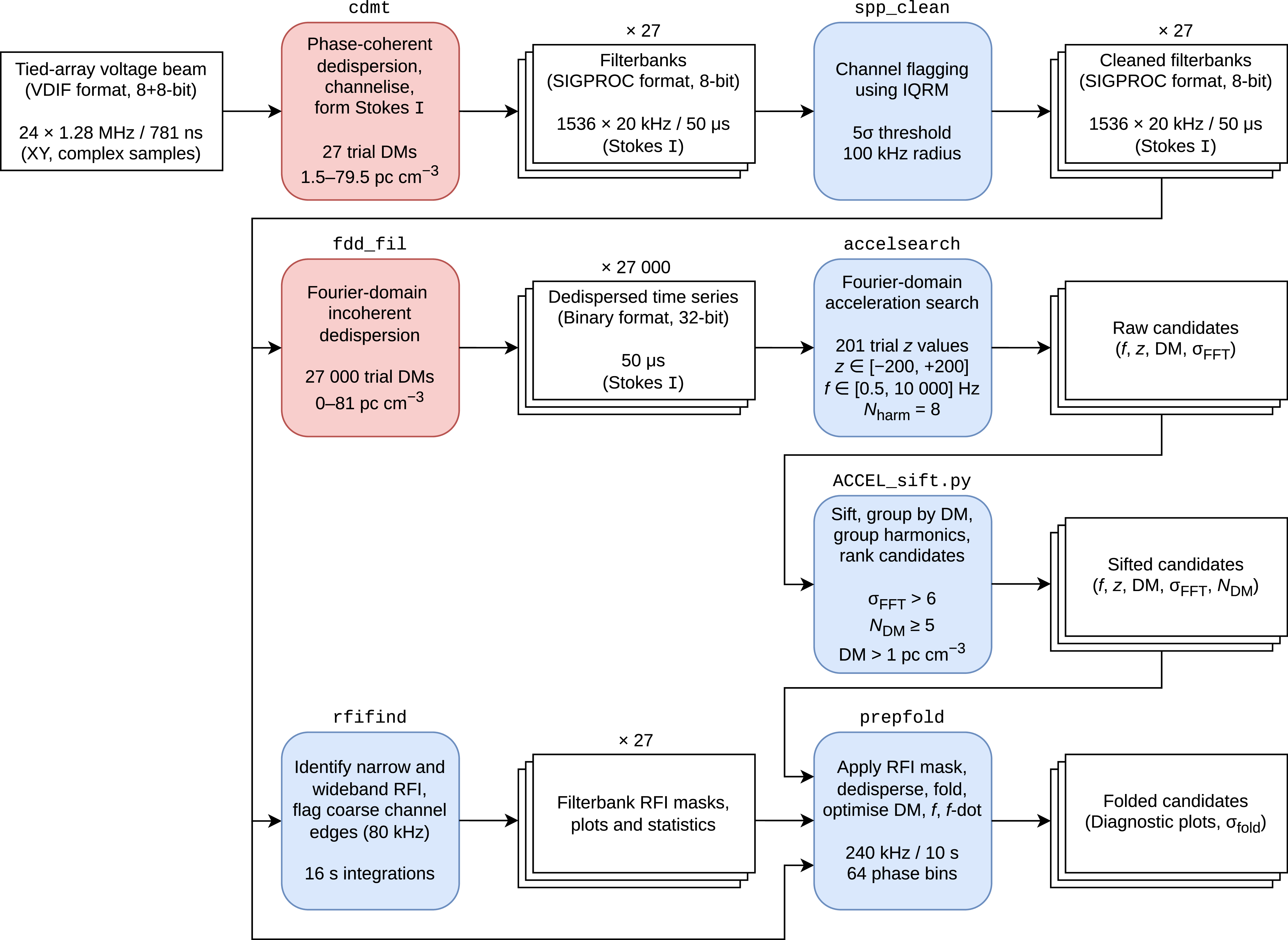
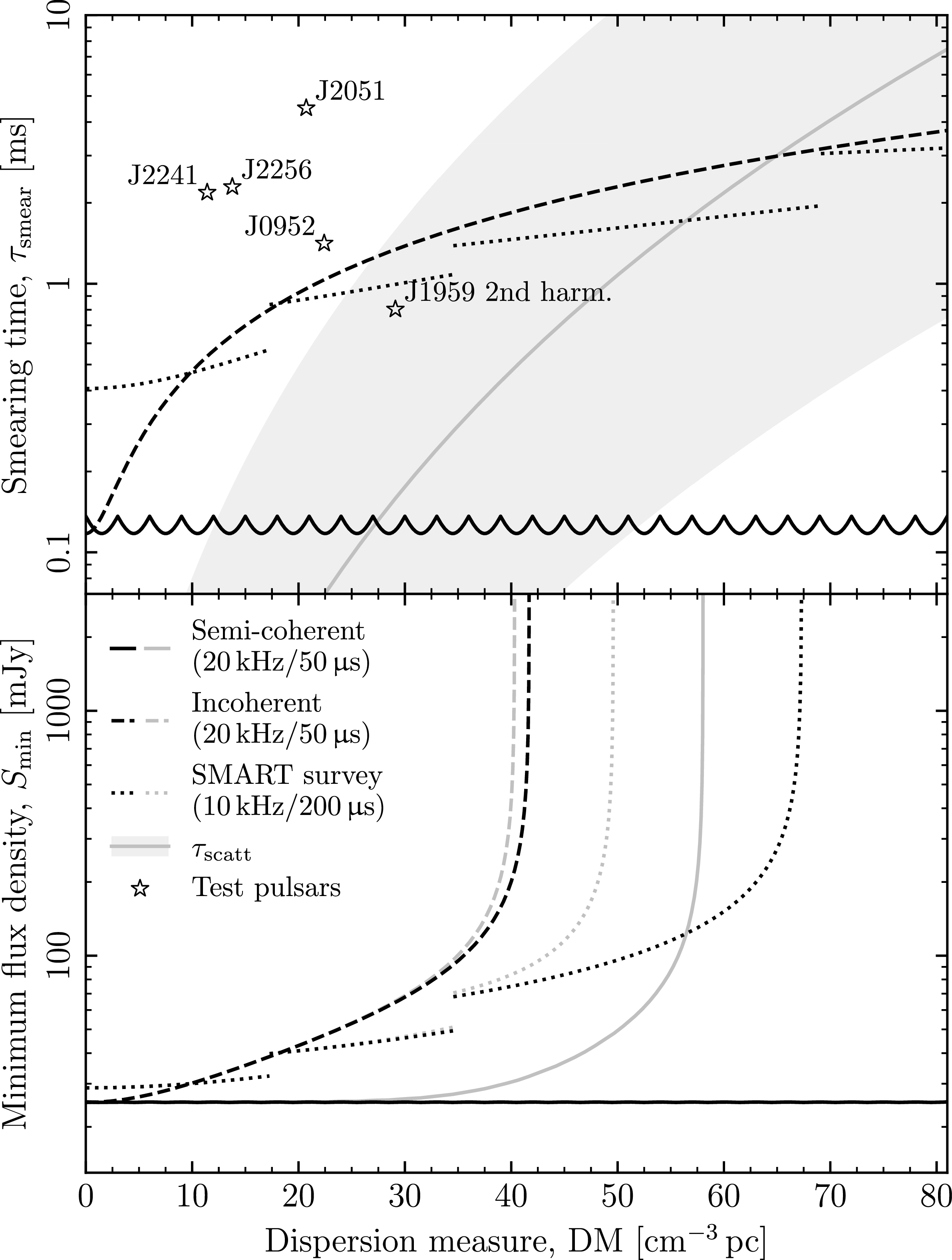
 138.88--169.60MHz
 τsmear
 τδDM
τδDM τscatt
 Smin
Smin 2ms
2ms 20min
20min 1kJy
1kJy Smin
Smin 20kHz
20kHz 50μs
50μs 0.003cm−3
 3cm−3
3cm−3 μ
μ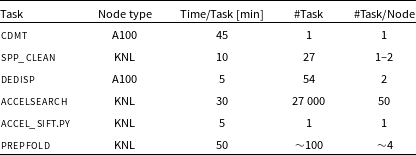
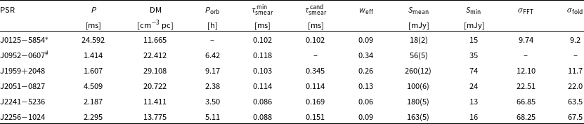
 Porb
Porb τsmearmin
 τsmearcand
 weff
weff Smean
Smean 154MHz
 Smin
Smin σFFT
σFFT σfold
σfold Smean
Smean Smin
Smin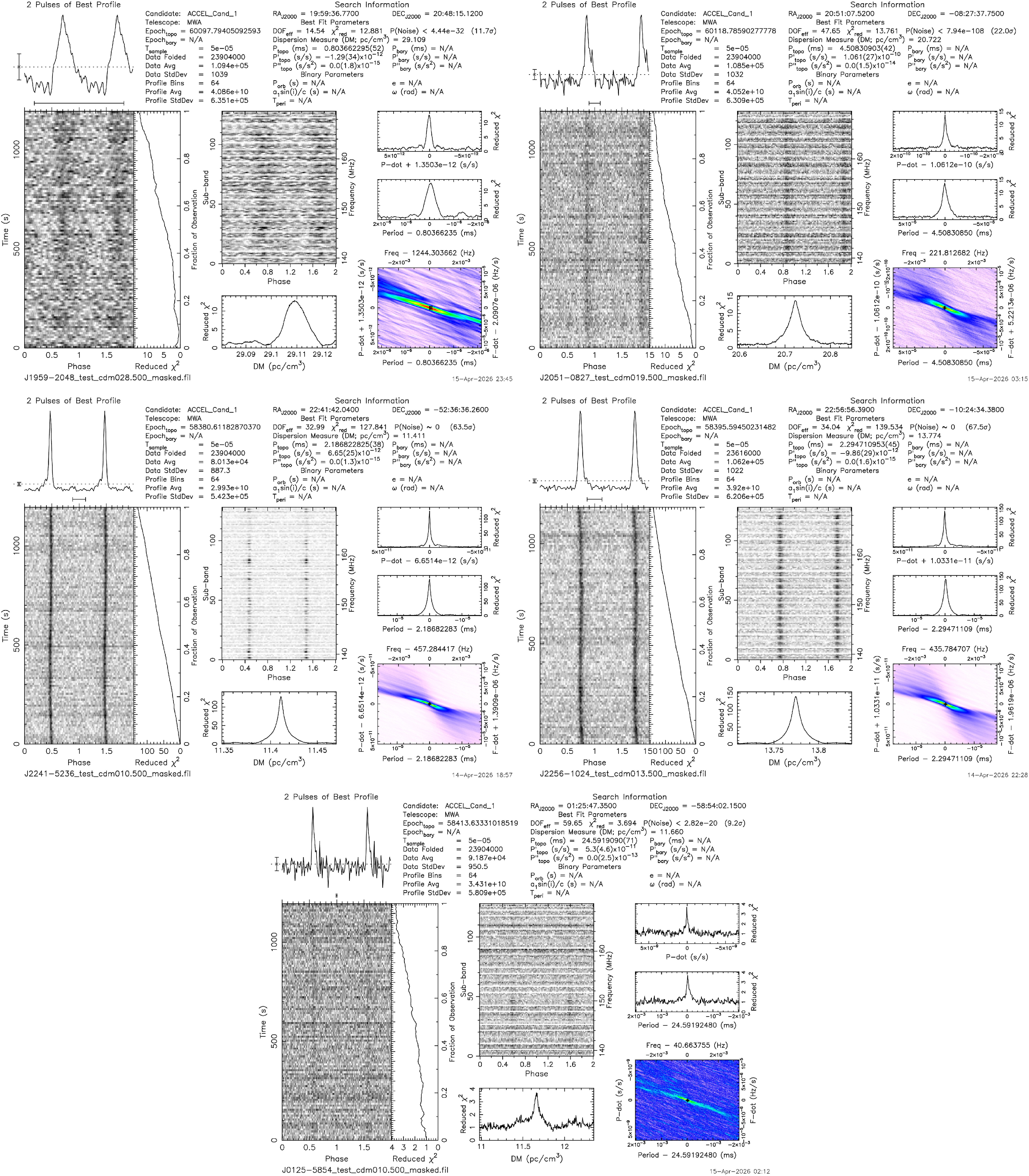
 −
− −
− −
− −
− χ2
χ2 P˙
P˙ P˙
P˙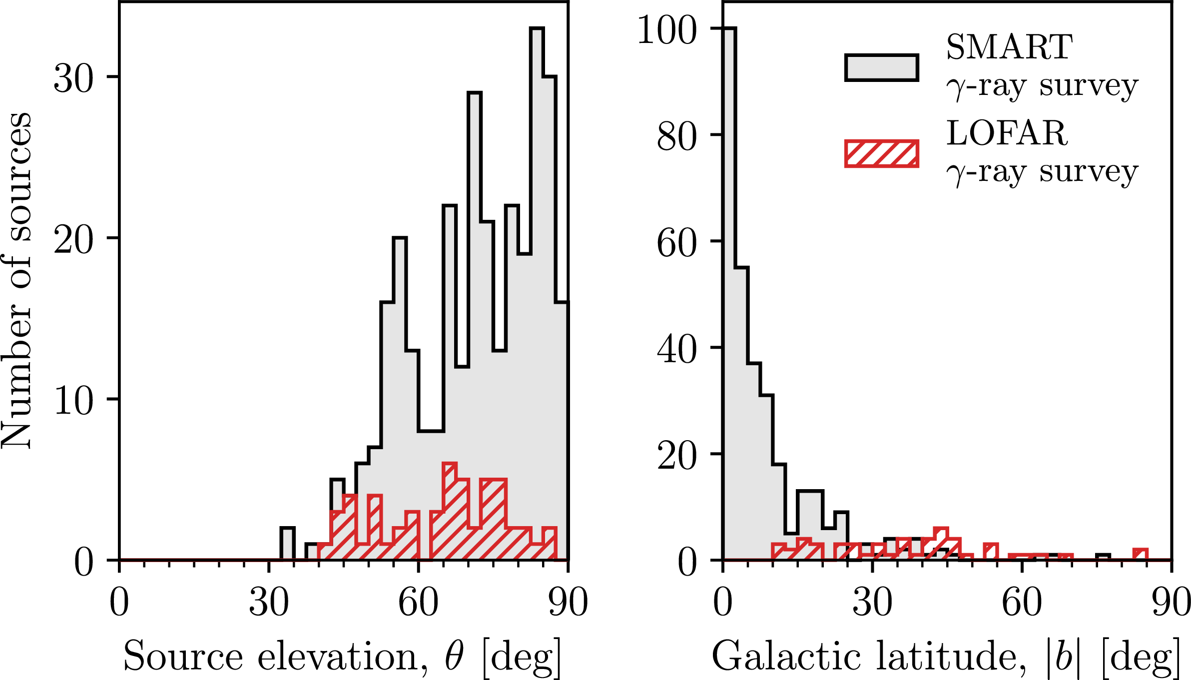
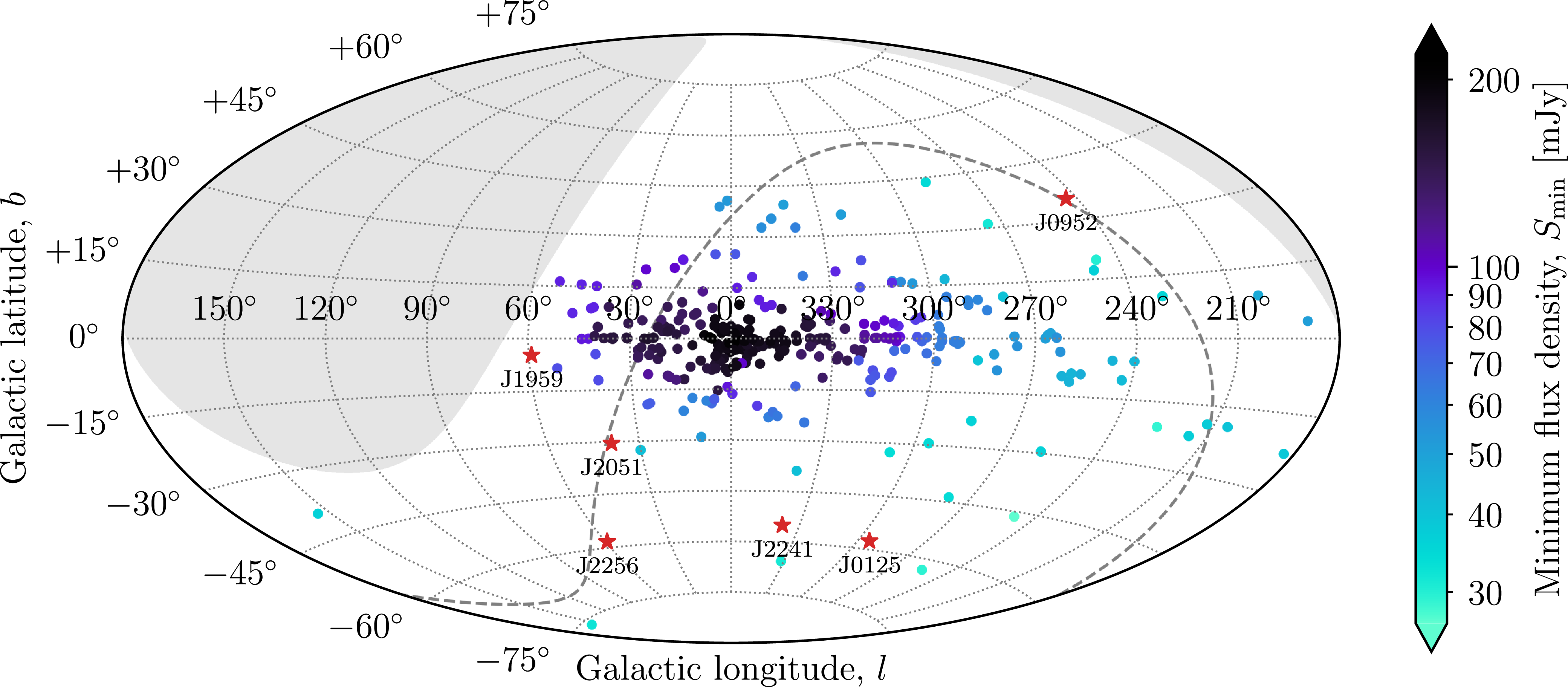
 Smin
Smin 2ms
2ms 20min
20min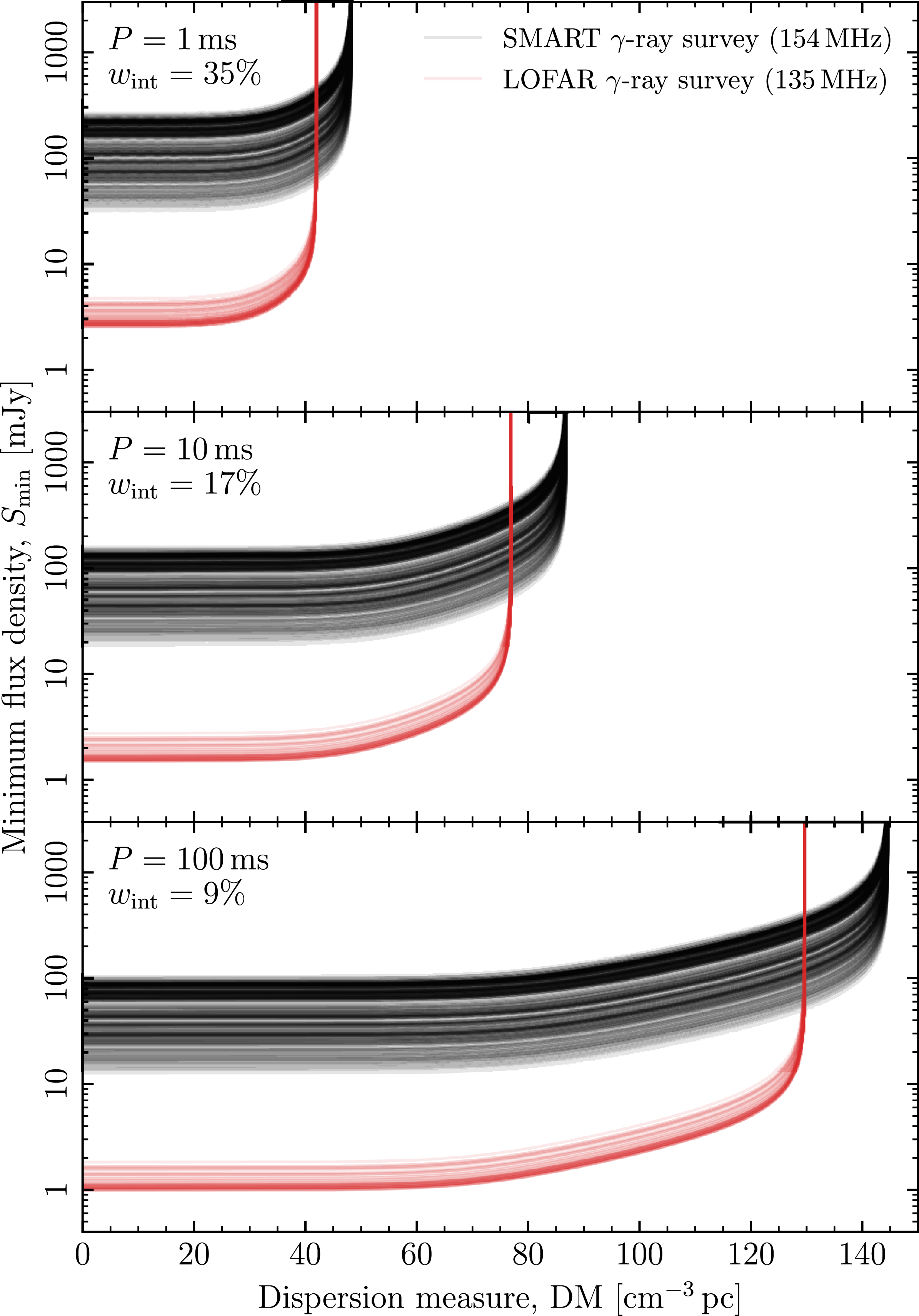
 154.24MHz
 100ms
100ms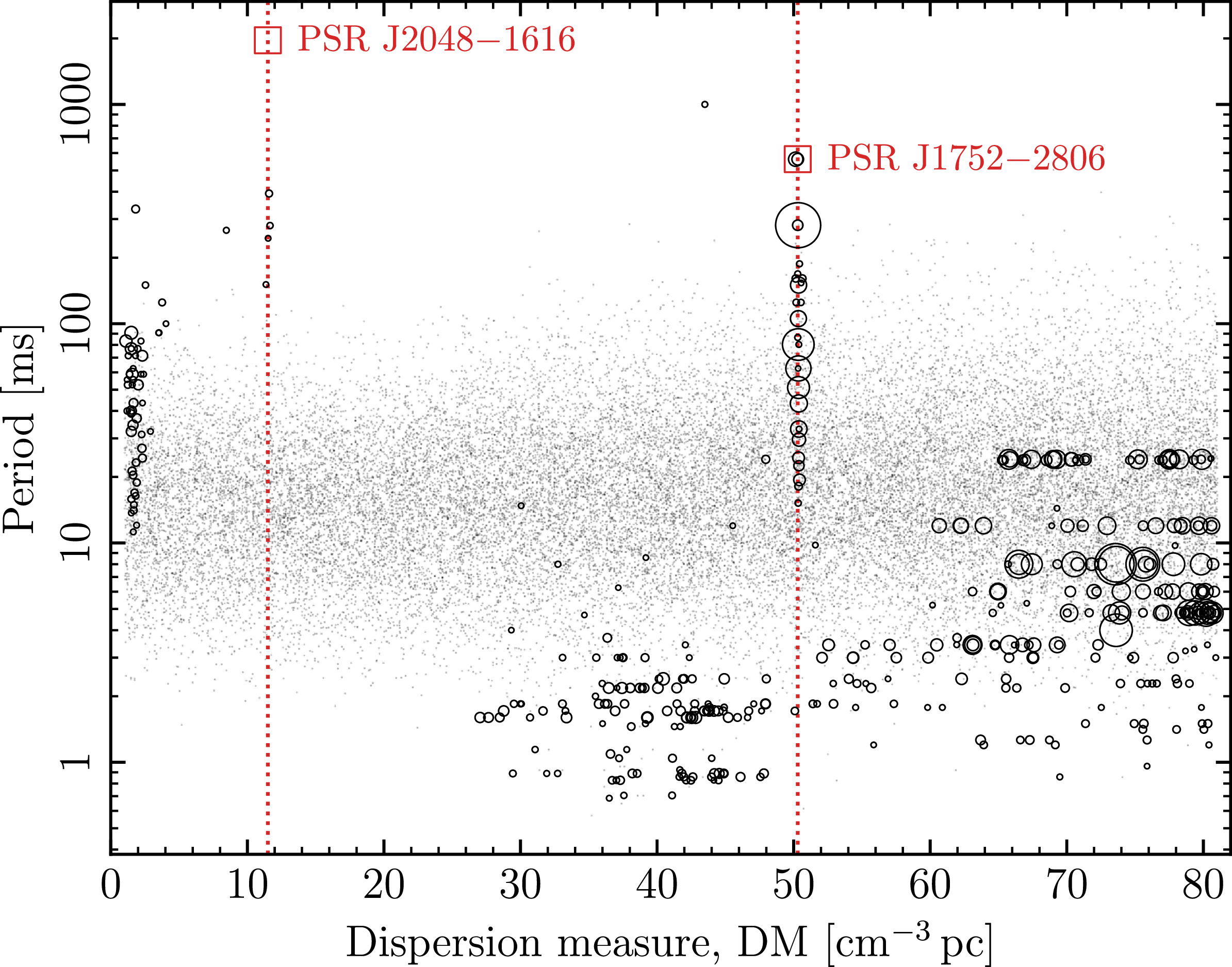
 σFFT>10
 σFFT
σFFT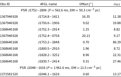
 σFFT
σFFT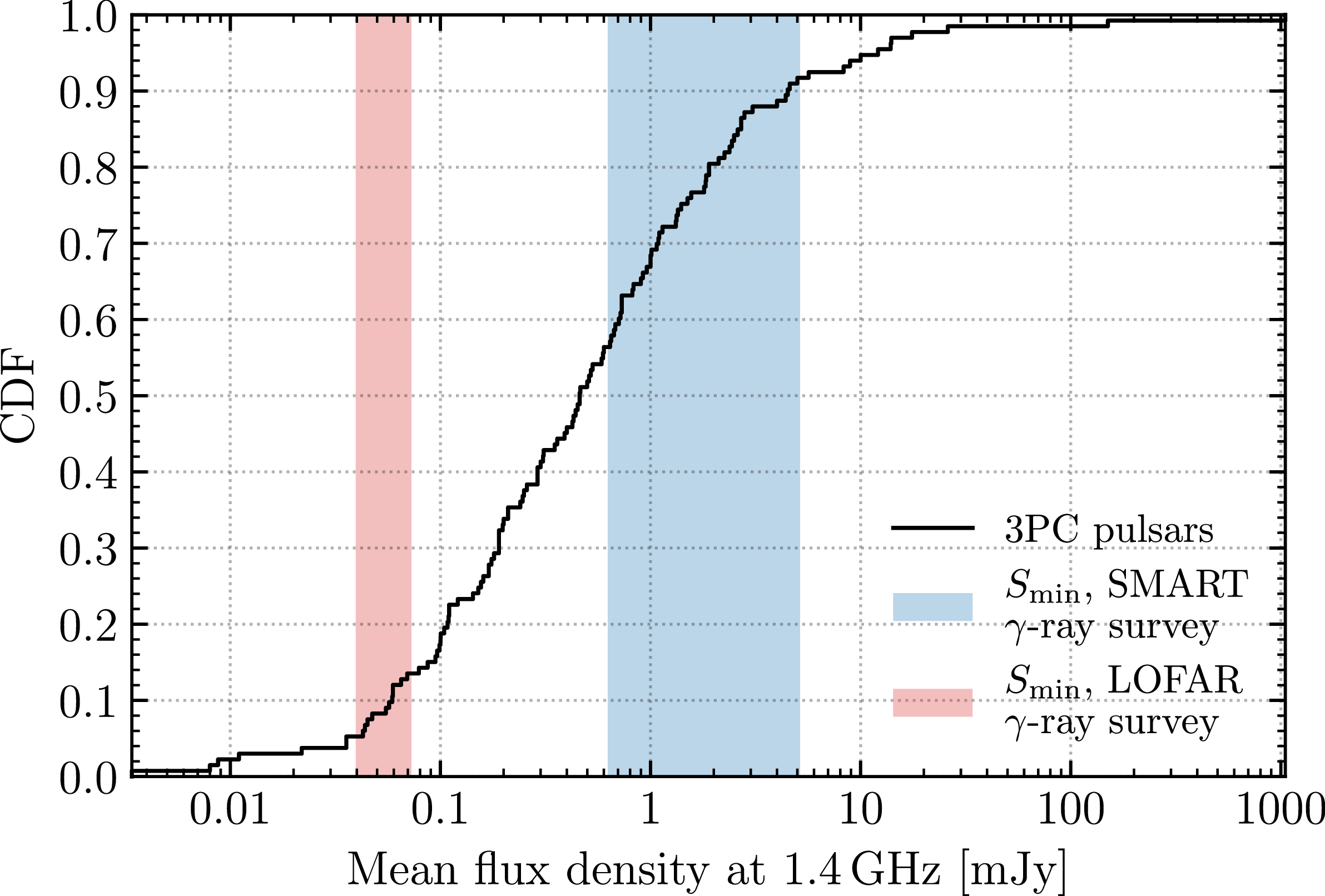
 1.4GHz
 100cm−3pc
 Smin
Smin 1.4GHz
 −1.7
−1.7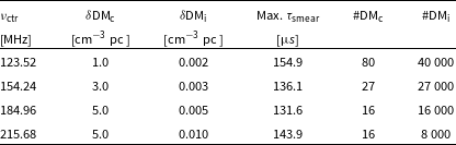
 30.72MHz
 50μs
50μs νctr
νctr δDMc,i
 τsmear
 80cm−3
 DMc,i
DMc,i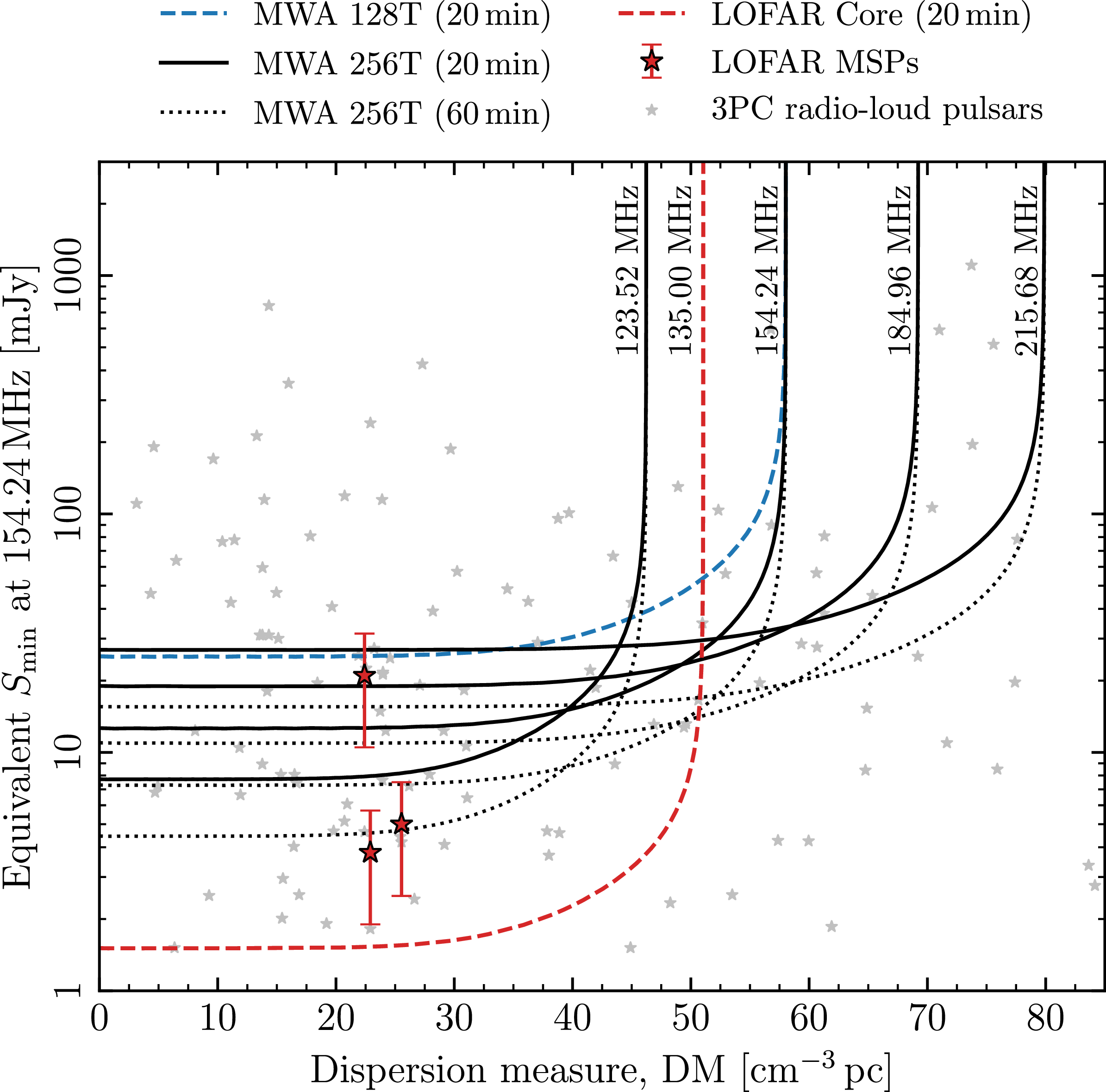
 154.24MHz
 2ms
2ms 154.24MHz
 −2.5
−2.5 154.24MHz
 135MHz
 20min
20min 60min
60min 150MHz
 −
− −1.7
−1.7
 r95
r95 θ
θ 154.24MHz
 2ms
2ms Smin
Smin
 Open access

