


1. Introduction
On the land-terminating regions of the Greenland ice sheet (GrIS), seasonal changes in meltwater delivery to the bed in the ablation zone drive large variations in surface motion that form a consistent annual velocity cycle (Joughin and others, Reference Joughin2008; Bartholomew and others, Reference Bartholomew2010; Hoffman and others, Reference Hoffman, Catania, Neumann, Andrews and Rumrill2011; Sole and others, Reference Sole2013; Moon and others, Reference Moon2014; van de Wal and others, Reference van de Wal2015; Andrews and others, Reference Andrews2018; Davison and others, Reference Davison, Sole, Livingstone, Cowton and Nienow2019, Reference Davison2020; Young and others, Reference Young2019). These flow variations are often interpreted in terms of changes in basal motion. However, deformation motion derived from shearing of the ice column also contributes to surface motion (Cuffey and Paterson, Reference Cuffey and Paterson2010), and the basal traction changes that modulate basal velocities are found to also impact the rate of deformation motion (Ryser and others, Reference Ryser2014a; Young and others, Reference Young2019). Variable deformation has similarly been observed on alpine glaciers undergoing transient forcing (Hooke and others, Reference Hooke, Pohjola, Jansson and Kohler1992; Willis and others, Reference Willis2003; Amundson and others, Reference Amundson, Truffer and Lüthi2006). Neglecting changes in deformational motion risks miscalculating the actual changes in basal motion, and thus, the sensitivity of basal motion to melt forcing at a given location. Moreover, the variability of deformation as it responds to a changing traction field can help distinguish whether ice flow variations through time are being forced locally, or are responding to traction changes elsewhere (Willis and others, Reference Willis2003; Amundson and others, Reference Amundson, Truffer and Lüthi2006; Ryser and others, Reference Ryser2014b; Young and others, Reference Young2019). Thus, timeseries measurements of deformation are important for determining the dynamic context of time-varying flow but are rarely quantified due to the difficulty associated with measuring englacial deformation.
The basal velocity field and its response to transient forcing is likely highly complex, controlled by hydrologic processes and bed topography that produce traction variations from meter to ice thickness length scales. The length scale of basal velocity variations observable at the surface is dependent on the basal slip ratio and thickness of the ice, but is generally greater than an ice thickness (Balise and Raymond, Reference Balise and Raymond1985; Gudmundsson, Reference Gudmundsson2003; Raymond and Gudmundsson, Reference Raymond and Gudmundsson2005). As a result, variability of basal motion at sub-ice thickness length scales that is critical to understanding of ice–bed coupling and its evolution during the melt season remain unobservable at the surface. Even at longer length scales, the use of surface velocities to investigate basal velocity patterns has fundamental limitations. Variability in the basal velocity is smoothed by changes in deformation motion through the ice column. Consequently, counter-intuitive surface velocity patterns can arise that do not reflect sliding variations across the bed (Gudmundsson, Reference Gudmundsson2003; Willis and others, Reference Willis2003; Ryser and others, Reference Ryser2014a). Given these uncertainties, it is often unclear how, if, or to what degree the smooth patterns of surface velocity are related to the detailed pattern of basal motion, making it difficult to infer the processes driving transient motion.
In this study, we investigate spatial and temporal variations in sliding and deformation motion over a nearly 2-year period using direct measurements made within a 3-D ice block in western Greenland's ablation zone (Fig. 1). We quantify ice motion and its different components using a five-station GPS network and eight inclinometry strings installed in a grid of boreholes drilled to the ice-sheet bed. These measurements allow for the direct partitioning of surface motion into sliding and deformation components at each borehole location. Using the data, we quantify the magnitude of sliding and deformation change, both seasonally and through the 2-year measurement period. We then examine the spatial pattern of sliding, deformation and surface velocities within the approximately ice-thickness scale borehole grid and investigate how these patterns change over an annual velocity cycle. Finally, we discuss the glaciological setting that would result in the spatiotemporal sliding and deformation variations we observe.
Site location, field instrumentation and boreholes configuration, and dynamic setting. (a) Field location, (b) plan view of borehole (14Sa – green, 14Sb – red, 14N – blue, 14W – purple, 15Ca – cyan, 15Cb – black, 15S – pink, 15E – orange, 15N – gray) and GPS locations, (c) 3-D view of borehole and instrument network with surface and smoothed bed topography (Lindbäck and others, Reference Lindbäck2014; Morlighem, Reference Morlighem2018). Right panels show the winter (d) and summer (e) velocity fields (Joughin and others, Reference Joughin, Smith, Howat, Scambos and Moon2010) for a 10 km × 10 km grid centered on the field location (measures quarterly velocities during 2015–2016). Gray contours delineate the underlying bedrock topography (Lindbäck and others, Reference Lindbäck2014; Morlighem, Reference Morlighem2018).

2. Site description
The field location is located ~34 km inland from the terminus of Issunguata Sermia, an outlet glacier located on the western margin of GrIS (Fig. 1). Winter surface velocities in the region are on the order of 100 m a−1 which is characteristic of land-terminating regions of the ice sheet (Joughin and others, Reference Joughin, Smith, Howat, Scambos and Moon2010) and can increase near twofold during summer flow (Fig. 1) (Joughin and others, Reference Joughin, Smith, Howat, Scambos and Moon2010). The site is located on a broad plateau in the bed topography with troughs located to the west (downgradient) and south (Fig. 1). The ice at the field site is ~670 m thick and borehole experiments indicate it is underlain by hard bedrock with no thick and deforming till layer present (Harper and others, Reference Harper, Humphrey, Meierbachtol, Graly and Fischer2017). Ice flow during winter is dominated by sliding; just 4% of the wintertime surface motion is accounted for by ice deformation (Maier and others, Reference Maier, Humphrey, Harper and Meierbachtol2019). The high-sliding fraction is facilitated by a basal boundary where ice flow and form drag over sparsely-spaced bedrock bumps of tens of meters in scale provide the resistance to sliding (Maier and others, Reference Maier, Humphrey, Harper and Meierbachtol2019). Pressure records show basal pressures remain consistently near overburden values, dropping only slightly during the melt season (Wright and others, Reference Wright, Harper, Humphrey and Meierbachtol2016). Borehole experiments have also identified locally isolated basal drainage conditions (Meierbachtol and others, Reference Meierbachtol, Harper, Humphrey and Wright2016) during the melt season, showing potential for water storage in discrete cavities at the site.
3. Field instrumentation
Individual inclinometer probes were constructed using two orthogonal high-precision analog inclinometers (Murata SCA103T) that measure tilt, θ, from vertical. Each inclinometer has a nominal resolution of 5 × 10⁻⁴° and a range of ±15° from vertical. The analog output from the inclinometers is measured by using a separate 24 bit A/D converter. The orientation of the inclinometer is measured by using a 3-axis magnetometer (Honeywell HMC5883) that has a resolution of 2°, and is lab calibrated with an eight-point calibration to ±10°. Near magnetic north, the magnetic field is inclined near close to vertical. Sensor orientations were thus retrieved by observing how the magnetic-field measurements change with tilting, and the inclinometer direction is estimated at a resolution of ±25° (Table 1). The inclinometer probes also have an onboard temperature sensor to measure englacial ice temperature. The temperature sensor (Texas Instruments TM102) has a resolution of 0.0625°C, is factory calibrated to ±1°C, and is lab and field calibrated to ±0.25°C. Each inclinometer package is embedded within a plastic cylinder using epoxy and constructed into inclinometry strings using CAT-5 cable.
Error and uncertainty for input parameters to calculate deformation and sliding velocity

The inclinometer strings were installed in nine boreholes drilled from the surface to the bed using hot water methods during the 2014 and 2015 summer. The boreholes were drilled in a grid, with an E–W and N–S extent of 465 and 280 m, respectively (Fig. 1). Borehole locations are denoted by the year they were drilled and the relative location within the borehole grid. Inclinometer strings were installed in each borehole immediately after drilling. The strings consisted of inclinometer probes spaced 10 m apart from 5–145 m above the bed and 20 m apart 145–625 m above the bed. At two borehole locations, 14Sb and 15Cb, only the bottom half of the ice column (<165 and <325 m above the bed, respectively) was instrumented with inclinometers. After installation, borehole refreezing mechanically couples the inclinometer probes to the ice. No thick temperate layer was observed with ice temperatures recorded below the pressure melting point extending down to at least ~5 m above the bed at all borehole locations (Hills and others, Reference Hills, Harper, Humphrey and Meierbachtol2017). Once installed, data were recorded continuously from each inclinometer string using a custom surface logger at 2- or 4-h intervals. At one borehole, 15N, no continuous tilt data were recovered after installation. Although the instrumented grid extends ~465 m along-flow, the ice also slides across the bed at a rate of ~100 m a−1 (Maier and others, Reference Maier, Humphrey, Harper and Meierbachtol2019). Thus, over the 2-year observational period the transport of our network across the bed by ice flow essentially extends our sampling area of the bed to approximately ice-thickness scale.
Surface position data used to calculate surface velocities was collected continuously at 15 s intervals from dual-band Trimble Net-R9 GPS receivers installed as an array at the field site (Fig. 1). The GPS array was installed in a four-point diamond with an additional station at the center, and the array spans an east–west and north–south distance of ~700 m. The position data from each GPS receiver is processed against a base station located ~22 km away using TRACK version 1.29 differential kinematic processing software.
4. Calculating deformation, sliding and surface motion
Inclinometers measure tilting which primarily arises from shearing. For an inclinometer installed near vertically in deforming ice, the rotation of the inclinometer from the vertical axis is related to the shear deformation in the direction of tilt (Keller and Blatter, Reference Keller and Blatter2012; Maier and others, Reference Maier, Humphrey, Harper and Meierbachtol2019):

where Δt spans the length of the period and θ is the tilt from vertical. Measurements made with a full-depth inclinometer string can be used to retrieve profiles of shear deformation (Fig. 2; Supporting data). Integrating these measurements through the ice thickness (H) yields an estimate of the deformation velocity (u d). When coupled with measurements of the surface velocity (u s) collected with the GPS array, sliding (u b) can be estimated at each borehole as the residual between the two motion components (u b = u s − u d). Surface velocities are calculated from GPS position data smoothed using a 5-d Gaussian kernel prior to differencing.
Example of deformation profile through annual velocity cycle. Deformation profile for borehole 15E (Fig. 1) is shown for the 2016 winter, 2016 early summer, 2016 late summer and 2017 winter. Each dot shows a du/dz measured by an individual inclinometer. Deformation profiles for other boreholes are included in the Supporting data.
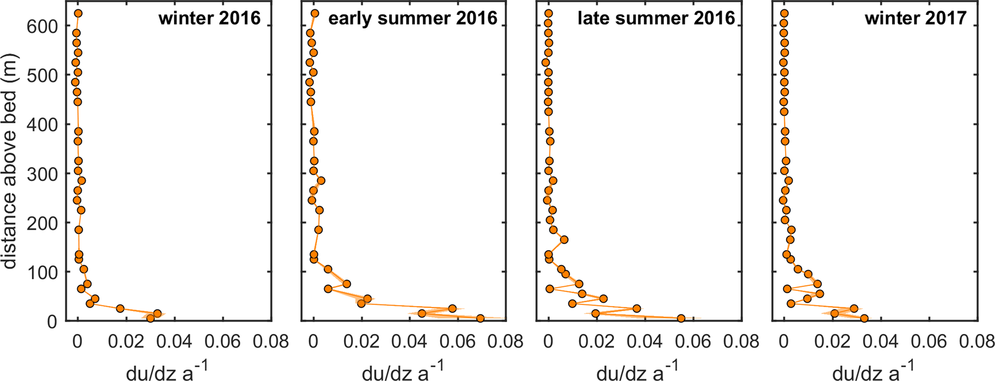
The thickness of the ice and location of the inclinometers within the ice column, which are needed to vertically integrate the shearing rates, changes as the ice thins or stretches vertically from the time of installation. The thickness of the ice at time t can be estimated using the longitudinal and transverse components of the strain tensor calculated from the GPS array as follows:

where ɛ xx,t is the total longitudinal strain in the x direction since the time of inclinometer string installation, ɛ yy,t is the total transverse strain in the y direction since the time of inclinometer string installation and H* is the ice thickness measured at each borehole location at the time of installation. The change in thickness is assumed to be distributed uniformly through the ice column. This treatment of thickness changes does not include depth-varying strain, however given the uniformly low-deformation rates in the upper half of the ice column (Maier and others, Reference Maier, Humphrey, Harper and Meierbachtol2019), this remains a reasonable approximation for much of the ice column. Localized thickness changes due to small-scale bedrock topography also occur at the field location (Maier and others, Reference Maier, Humphrey, Harper and Meierbachtol2019) and are included in the uncertainty estimate provided in Table 1.
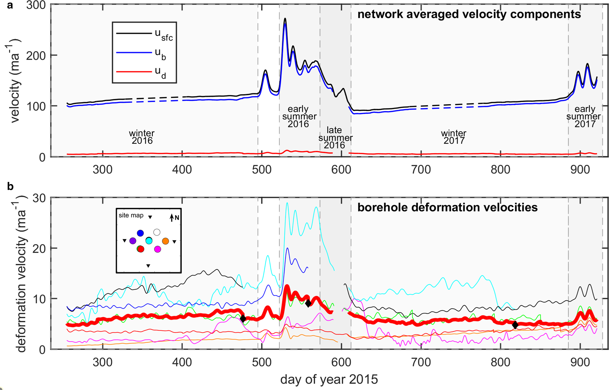
Using the above equations, we calculate deformation, sliding and surface velocities at each borehole location across a 2-year period (2016–2017). A continuous record of the surface, sliding and deformation motion at the site is presented in Figure 3. For our analysis, we focus on the motion components estimated across longer time periods that reflect major periods of an annual velocity cycle (winter, early summer, late summer). These are shown in Figure 4 and the relevant characteristics of each period are detailed in Table 2. This is done for several reasons: (1) spatial patterns in motion during periods relevant to our annual dynamics can be easily examined. (2) Longer Δt is needed to resolve the englacial rates above their noise threshold due to exceptionally low-deformation rates observed at the site (Maier and others, Reference Maier, Humphrey, Harper and Meierbachtol2019). (3) Localized positive and negative tilt variations observed as the ice slides over roughness (Maier and others, Reference Maier, Humphrey, Harper and Meierbachtol2019) are averaged out over longer time periods, and thus the changes in the deformation and sliding velocities are less likely to be influenced by short-length scale roughness observed to be common at the site. Because of this effect, the continuous records shown in Figure 3 do not include the basal most sensor which show a high variability even during winter as the sensors transit basal roughness features.
Time series of velocity components. (a) Network-averaged velocity components (5 d) are plotted for deformation, sliding and surface velocity. (b) Deformation velocity time series (5 d) is plotted for each borehole with continuous data during the measurement record. Thick red line shows the average deformation velocity from all boreholes. Diamonds indicate string failures which change the number of boreholes in the average. The inset panel shows borehole locations. Vertical dashed lines indicate major time periods investigated in study.
Sliding velocity, deformation velocity and percentage change in each between measurement periods. In panel (a), the sliding velocity across each measurement period at each borehole location is displayed. The colors correspond to the borehole locations shown in Figure 1 and site map inset. Panel (b) shows the deformation velocity across each measurement period for all borehole locations. For the top two panels vertical gray error bars indicate ±σ of combined error and uncertainty. If no lines are present, the error is smaller than the marker size. Panel (c) shows a box plot of the percent change in deformation velocity (red box) and sliding velocity (thin blue box) from period to period. The vertical width of the boxes indicates the interquartile range, the whiskers the range and the blue line within the box the median. Boxes without whiskers have statistical outliers on the end of the range.

Period characteristics

The chosen periods (Fig. 3) capture the major features of the annual velocity cycle which are commonly interpreted to reflect changing subglacial hydrology (Bartholomew and others, Reference Bartholomew2010; Andrews and others, Reference Andrews2018; Davison and others, Reference Davison, Sole, Livingstone, Cowton and Nienow2019). The winter period captures conditions outside of the melt season when there is no surface melt and surface velocities are relatively stable. The early summer captures the initial acceleration and elevated shoulder of the melt season, and late summer captures declining velocities observed during of the latter half of the melt season. For ease of identification throughout the manuscript, the winter periods where no surface melting occurs will be described using a single year and descriptor (i.e. 2016 winter), despite spanning portions of both years temporally and different calendar seasons (i.e. fall, winter and parts of spring, Fig. 3). The year used corresponds to the year of the subsequent melt season, i.e. the 2016 winter precedes the 2016 melt season.
4.1 Estimating uncertainty
We perform a Monte Carlo simulation through the deformation and sliding calculations to generate robust uncertainty estimates needed to compare small spatiotemporal variations in ice motion observed at the site. Monte Carlo is a probabilistic method used to estimate uncertainty through complicated equations whereby fully exploring the error distribution of the input parameters through many iterations the uncertainty of the output parameter can be determined. In our Monte Carlo simulation, 10 000 iterations of the deformation and sliding calculations were performed at each borehole and over each period. Each iteration is initialized by a random set of input values derived from the error and uncertainty distributions of each input parameter which are quantified in Table 1. Compilation of the results from all iterations yields a probability density function (PDF) for the deformation and sliding velocity at each borehole. Output PDFs of the deformation, sliding and surface velocities approximate a normal distribution, and we describe their values using the mean and uncertainties by the std dev.
We find the uncertainty in magnetic orientation and rotational uncertainty induced by normal strains dominate all other sources of error and uncertainty and are both on the order of 10% of the deformation velocity (total error and uncertainty shown in Fig. 4). Comparatively, instrumental error for the tilt sensors and GPS receivers, as well uncertainty in the ice thickness and vertical strain, contribute a negligible amount to the overall uncertainty in deformation and sliding.
4.2 Treatment of basal inclinometer failures
Many inclinometer strings functioned for multiple years demonstrating remarkable durability during the field experiment. Even so, some inclinometers near the bed lost functionality at some point during the measurement period (Supporting data) presumably due to stretching of the cable from cumulative strain or high-ambient pressures. In an effort to maintain comparable records of the deformation and sliding velocity through the measurement period, we estimated the deformation rates for any basal inclinometers that failed prior to the end of the 2-year measurement period. This was done by fitting a third-order polynomial to the deformation rates through the ice column and extrapolating the fit to the failed inclinometer depth. Using a polynomial as opposed to a power law was done in an effort better approximate some of the more complex behaviors observed near the bed at some boreholes (i.e. basal deformation kinks, Supporting data). This polynomial is generated for every iteration of the Monte Carlo simulation. The uncertainty of the measurements used for the polynomial fits combined with the flexibility of the polynomial results in a wide range of estimated values (Supporting data) through the Monte Carlo simulation (Supporting data). Thus, even though we cannot explicitly quantify the uncertainty, we can use the spread of the extrapolated deformation rates as an estimate of uncertainty. We note, although that extrapolation was mainly used to estimate the values of the basal-most inclinometer, due to multiple inclinometer failures at 14N directly prior to string failure (Supporting data), extrapolation was used for the bottom 50 m of the ice column during the 2016 early summer period.
5. Results
5.1 Temporal changes in ice motion
We present continuous and period-averaged deformation and sliding records in Figures 3 and 4, respectively. We find that sliding dominates ice motion and almost always contributes >90% of the total ice motion regardless of the period or borehole location. In general, sliding and deformation motion covary positively over the 2-year period, where changes in deformation motion track sliding even through the melt season. A statistical representation (interquartile range and median) of the percent velocity change between periods for deformation and sliding (Fig. 4) corroborates this, showing positive covariation of deformation and sliding through an annual cycle. We observe a large increase in the sliding (67%) and deformation velocity (119%) from the winter to the early summer in 2016. The increase in deformation is more variable between borehole locations than is sliding. The positive covariation of deformation and sliding continues from early to late summer and from late summer to the subsequent winter. From early to late summer, the sliding velocity decreases by 32%, while the deformation motion decreases by 21%. The change in deformation motion during this period is much more uniform across the borehole network. Transitioning from late summer to winter a nearly equal decrease (~50%) is observed for both components of motion. Similar to the 2016 melt season, large increases in both sliding and deformation velocities occur from winter to the early melt season in 2017, showing consistency in the temporal behavior between the two years. In general, deformation changes in the basal 200 m of ice are the primary source of deformation variability through time (Fig. 2; Supporting data).
5.2 Spatial relationship between sliding, deformation and surface velocity
In Figure 5, spatial patterns of deformation, sliding and surface velocity are presented for an annual velocity cycle (2016 winter to 2017 winter). Here, the spatial patterns are presented as period-specific velocity anomaly, where the mean velocity component (i.e. surface, deformation or sliding) calculated from all borehole locations is subtracted from that measured at individual boreholes to emphasize spatial gradients.
Velocity patterns within borehole network through an annual velocity cycle. Each plot shows a map view of the field site plotted in local coordinates. The surface velocity anomaly (interpolated surface in background), deformation velocity anomaly (inner squares) and sliding velocity anomaly (outer circles) are show through a full seasonal cycle (2016 winter to 2017 winter, panels (a) through (d) within the borehole network. The circles and squares correspond to the borehole locations in Figure 1 (only boreholes with functioning inclinometry strings are shown). Velocity anomalies are calculated by subtracting the site mean velocity component (surface, deformation or sliding) from that measured at each location for each period. Distance is referenced to the center GPS position at time of installation in the 2014 melt season. The borehole grid is moving approximately east to west (right to left) which is shown in the figure sequence.
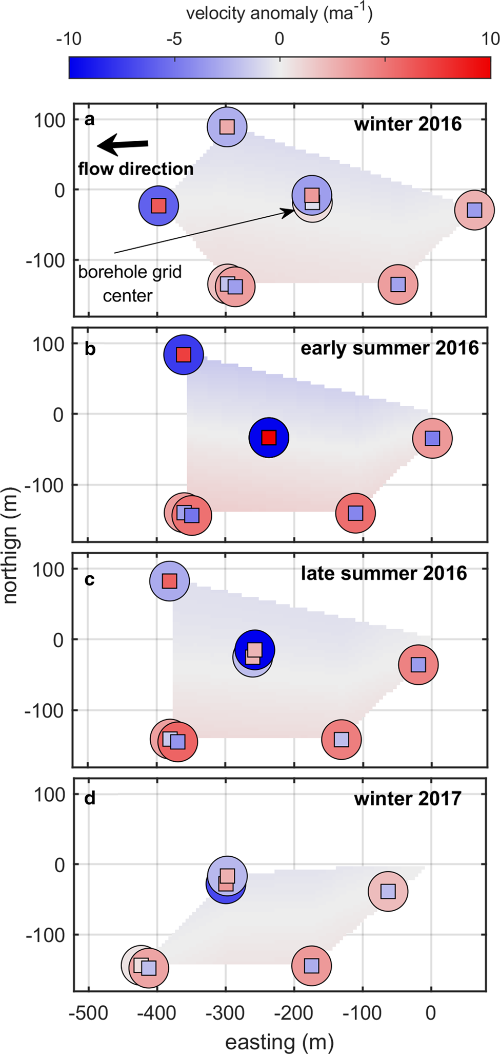
We first examine the 2016 winter, when eight inclinometry strings were simultaneously operational yielding the most complete spatial coverage across the borehole grid during the measurement record. During this period, we find the surface velocity pattern has slight N–S gradients (~1.8 m a−1 north to south difference) with lowest and highest velocities recorded on the northern and southern sides of the field location, respectively. In comparison, the deformation and sliding fields have much stronger gradients that trend NE–SW (~8 m a−1 northeast to southwest difference). Although small in terms of velocity magnitude, this represents an eightfold difference in deformation motion across the borehole grid. The highest rates of deformation are in the west and northwestern portions of the borehole grid and the lowest those on the eastern and southern sides of the grid. The sliding motion varies inversely compared to deformation motion, i.e. the sliding pattern is opposite the deformation pattern. Correspondingly, the highest sliding values are present in the southern and eastern portions of the borehole grid, and the lowest are in the western and northern regions of the grid. Because of the inverse relationship between the sliding and deformation fields the resulting surface gradients are comparatively muted, and only subtly resemble the sliding gradients measured at the bed.
Continuing through the remaining periods we find similar surface, sliding and deformation patterns across the borehole network (Fig. 5). After the 2016 winter, the spatial coverage across the borehole network decreases as certain inclinometer strings within the network failed. However, over the common portion of the borehole grid, the sliding and deformation patterns show only minor variation through time, and the gridscale NE–SW deformation and sliding gradients persist through the entire measurement period.
5.3 Borehole clustering
Both the timeseries (Fig. 4) and spatial patterns of sliding and deformation (Fig. 5) show that the transition between the high and low deformation and sliding velocities across the borehole grid is abrupt. The sharp transition between the highest and lowest velocities across the site is best characterized as clustered, where the deformation is either high or low (relative to mean of all boreholes). The boreholes within each cluster generally reflect the positive and negative velocity anomalies presented in Figure 5, where the low deformation and high sliding occurs on the southeast portion of the borehole grid, and the high deformation, low sliding occur on the northwestern portion of the borehole grid. The clustering persists through the measurement period due to the positively covarying deformation and sliding (Figs 3, 4) which causes the ratio of sliding to deformation to remain relatively stable through time. Accordingly, plotting the ratio of sliding to deformation for all periods (Fig. 6) yields graphically distinct plotting regions for the negative and positive velocity anomalies (anomalies indicated for deformation), which also have distinct trajectories in the sliding to deformation ratio through an annual velocity cycle indicating there are distinct and characteristic seasonal velocity changes that occur within each cluster.
Clustering of boreholes based on sliding and deformation trajectory. Sliding and deformation velocity is plotted against each other for all time periods and borehole locations. Marker colors correspond to deformation velocity anomaly (see also Fig. 5) calculated for each time period. Winter, early summer and late summer periods are indicated by marker type. Dashed lines show linear fit to data with deformation velocity anomaly higher or lower than zero which roughly delineates the clustered regions. The lower fit has R 2 = 0.22 and p = 0.048, the upper fit has an R 2 = 0.65 and p < 0.01.

6. Interpretation and discussion
Our previous study at the field site found sliding-dominated motion during winter (Maier and others, Reference Maier, Humphrey, Harper and Meierbachtol2019). Detailed tilt observations and numerical modeling tied the high-sliding fraction to the driving stress being resisted by form drag around sparsely spaced bed asperities tens of meters in scale (Maier and others, Reference Maier, Humphrey, Harper and Meierbachtol2019). The data here expand on this study and present a picture of ice flow at longer length scales approaching an ice thickness and spanning both winter and summer conditions. It is important to note that the observations identified above are integrated over longer periods during which shorter timescale variations occur (Fig. 3). Thus, the measurements reflect the mean state during the periods investigated and not a specific flow pattern at any snapshot in time.
6.1 Stability of the sliding and deformation fields
The unique observations of a sub-ice thickness scale sliding and deformation fields (Fig. 5) are made possible by the dense network of inclinometers installed at the field location. We find that the basic spatial velocity pattern persists through the seasonal velocity cycle and the 2-year measurement period. The clustering of high and low velocities indicates that the borehole grid straddles a relatively sharp transition between two regions with different motion characteristics.
Although the spatial variation in sliding velocity is small in magnitude across the borehole network, the spatial deformation variations show an approximate order of magnitude differences during any given measurement period (Figs 4, 5). Temperature measured in boreholes across our site show a nearly 2°C difference at similar depths across the borehole grid (Hills and others, Reference Hills, Harper, Humphrey and Meierbachtol2017). Such temperature differences suggest a maximum change of ~30% in the deformation rate factor, and thus cannot account the variation in deformation motion recorded across the study site alone. Correspondingly, the deformation gradients across the borehole network likely arise from a significant basal traction differences across the area of the borehole network. Assuming the site has an ice rheology with a creep exponent equal to three and an ice softness (controlled by ice temperature, impurity content, grain size, etc.) that does not vary more than expected via the measured temperature gradients, the gradients in deformation motion reflect an approximate twofold change in basal stress between the high- and low-deformation velocity regions. However, since we cannot explicitly account for the effective stress from normal components of the stress tensor, we consider this basal stress estimate to approximate a maximum end member.
It is plausible that the stress differences across the borehole network and ensuing sliding and deformation pattern could result from spatial variations in the basal substrate, small-scale roughness (tens of meters scale), hydrologic properties at the bed, larger scale topographic variations (hundreds of meters or greater), or traction gradients caused by coupling to far-field flow. All drilling observations from the nine boreholes drilled to the bed indicate a hard bed (Harper and others, Reference Harper, Humphrey, Meierbachtol, Graly and Fischer2017), yielding no evidence for a major change in substrate across the borehole grid. A previous study found roughness (1–10 m scale) induced near-basal tilting variations in both the high- and low-deformation regions of the study area (Maier and others, Reference Maier, Humphrey, Harper and Meierbachtol2019). Therefore, spatial variations in small-scale bed roughness are unlikely to have primary control on the spatial patterns observed. The presence of a persistent moulin indicates that meltwater can access the bed to the south of the study site (~100 m south of the southern GPS station, Fig. 1). It is unclear how the introduction of water at a nearby point at the bed would influence the traction field across the study area, and during an entire year. However, the time variations in deformation do not reflect a classical pattern of traction variability associated evolving seasonal drainage within actively forced regions of the bed, i.e. acceleration caused by decreasing traction, deceleration caused an increase in traction (Bartholomew and others, Reference Bartholomew2010; Andrews and others, Reference Andrews2018; Davison and others, Reference Davison, Sole, Livingstone, Cowton and Nienow2019). Thus, we have limited evidence to tie the spatial pattern to spatial changes in hydrologic characteristics of the bed.
Comparison of bed topography within the study area shows that the borehole network is sliding over the southern side of an elongated ridge that rises slightly in the along-flow direction, and results in a ~50 m difference in bed elevations between the southeastern and northwestern portions of the borehole grid (Figs 1, 7). This trend mimics the spatial sliding and deformation pattern, suggesting that the spatial pattern we observe arises from dynamics associated with oblique ice flow over the ice-thickness-scale bed topography. This hypothesis is physically plausible; the stoss sides of topography will support some of the driving stress, and therefore would have more deformation than the lee side or flat areas of the bed with comparable roughness (Kyrke-Smith and others, Reference Kyrke-Smith, Gudmundsson and Farrell2018). However, we cannot discount the possibility that stress–gradient coupling to differentially moving ice flow around the site could also influence the sliding and deformation pattern observed.
Spatial relationship between sliding fraction and bed topography. Bed elevation (brown surface, smoothed) is plotted with sliding fraction for each period and borehole location overlain (circle markers). Approximate ice flow direction is toward the positive along-flow distance values.

6.2 Positively covarying sliding and deformation motion
The large seasonal speed-up we observe during the melt season is consistent with many previous studies that have established the sensitivity of GrIS ice flow to seasonal meltwater inputs (Joughin and others, Reference Joughin2008; Bartholomew and others, Reference Bartholomew2010; Hoffman and others, Reference Hoffman, Catania, Neumann, Andrews and Rumrill2011; Sole and others, Reference Sole2013; Moon and others, Reference Moon2014; van de Wal and others, Reference van de Wal2015; Andrews and others, Reference Andrews2018; Davison and others, Reference Davison2020). The previous assumption that such seasonal speed-ups resulted primarily from sliding (Zwally and others, Reference Zwally2002; Bartholomew and others, Reference Bartholomew2010) has more recently been refined by measurements of time-varying shear (Ryser and others, Reference Ryser2014a, Reference Ryserb; Young and others, Reference Young2019), which have demonstrated that transient deformation is a common feature of summer ice flow in Greenland. Similarly, time-varying deformation is found during transient forcing on alpine glaciers indicating this behavior is not unique to large ice sheets (Hooke and others, Reference Hooke, Pohjola, Jansson and Kohler1992; Willis and others, Reference Willis2003; Amundson and others, Reference Amundson, Truffer and Lüthi2006). Combined, these measurements indicate time-varying deformation is relatively common. This fact is unsurprising, ice deformation and basal motion are inherently linked to the basal traction (Cuffey and Paterson, Reference Cuffey and Paterson2010), and are thus both sensitive to changes in ice–bed coupling that occur in response to melt forcing (Iverson and others, Reference Iverson, Hanson, Hooke and Jansson1995; Bartholomaus and others, Reference Bartholomaus, Anderson and Anderson2008).
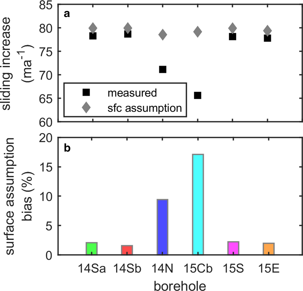
Our data are consistent with these findings, and additionally show that deformation motion can change in consistent and predictable ways through an annual velocity cycle (Figs 3, 4). Deformation and sliding changes scale with each other. Thus, the time variations in sliding, and correspondingly, the sliding sensitivity to transient forcing, are both lower than would be inferred assuming changes in surface motion reflect changes in sliding (i.e. surface assumption, Fig. 8). Using the data at our site we show using the surface assumption to estimate sliding changes moving winter to summer flow results in a 1.5–17% bias in the inferred sliding velocities across the borehole network (Fig. 8). Although the deformation velocity comprises only a small fraction of the surface motion at our site, in regions where the deformation fraction is higher, covarying sliding and deformation may result in a speed-up that is in large part due to changes in deformation motion. This effect is locally demonstrated within our borehole network (Figs 4, 8). Boreholes with higher initial deformation fractions have a higher fraction of the surface velocity change due to deformation.
Inferred sliding bias from surface assumptions. (a) The measured sliding increase moving from the 2016 winter to the 2016 early is shown for each borehole location (black squares). The inferred sliding increase estimated assuming all changes in surface motion reflect changes in sliding (i.e. surface assumption) is also shown (gray diamonds). (b) The percent difference between the sliding increase measured and inferred using the surface assumption (i.e. surface assumption bias) at each borehole location is plotted.
Positive covariation of sliding and deformation motion through an annual velocity cycle has not been previously observed and thus its dynamic context is not yet established. Our findings contrast observations made on an alpine glacier in Switzerland by Willis and others (Reference Willis2003) which found no consistent relationship between sliding and deformation changes through an annual cycle at multiple borehole locations. This was inferred to be the result of complex spatiotemporal traction changes at the bed, where tractions beneath the borehole locations were inferred to be local or non-locally modulated at different points in the melt season (Willis and others, Reference Willis2003). However, in Greenland, covarying deformation was previously observed (Ryser and others, Reference Ryser2014b), but across much shorter timescales (diurnal and 10 d) than our study. Using numerical models, this was interpreted to be consistent with traction changes mainly induced via stress–gradient coupling to flow variations elsewhere (i.e. a dynamically passive response).
Similar to this study, we posit the coupled sliding and deformation demonstrated by our observations across the seasonal scale is also consistent with traction changes mainly induced via stress–gradient coupling which would impact sliding and deformation similarly (Price and others, Reference Price, Payne, Catania and Neumann2008; Ryser and others, Reference Ryser2014b). Moreover, we would expect local traction variations associated with meltwater forcing within the borehole grid would reorganize the seasonal spatial pattern of sliding and deformation. Yet, this is inconsistent with our observations, and suggests local changes in the traction due to hydrologic forcing do not have a primary role in the spatiotemporal variations observed at the site. Therefore, the spatiotemporal evidence suggests our site is mainly responding passively to transient forcing originating from outside of the borehole network during the 2-year period. This hypothesis is consistent with direct borehole observations at the site, where isolated drainage conditions (Meierbachtol and others, Reference Meierbachtol, Harper, Humphrey and Wright2016) and water pressures near overburden during both summer and winter flows (Wright and others, Reference Wright, Harper, Humphrey and Meierbachtol2016) were measured. Yet, given the time-integrated nature of observations, and the hypothesized influence of the local bed topography on the sliding pattern, we cannot rule out that the site is locally forced over shorter timescales, or that changing basal resistance as sliding speeds vary over the local bed topography mask local forcing due to changing subglacial hydrology.
The conceptual model of seasonally evolving subglacial drainage in land-terminating regions implies that deformation motion which would inversely vary with sliding within actively forced regions of the bed (Bartholomew and others, Reference Bartholomew2010; Andrews and others, Reference Andrews2018; Davison and others, Reference Davison, Sole, Livingstone, Cowton and Nienow2019). At the onset of melt and early summer, decreased ice–bed coupling occurs as water flows through distributed drainage (Bartholomaus and others, Reference Bartholomaus, Anderson and Anderson2008; Bartholomew and others, Reference Bartholomew2010), while during late summer, an increase in drainage efficiency increases coupling and traction leading to the commonly observed late summer slowdown (Bartholomew and others, Reference Bartholomew2010; Andrews and others, Reference Andrews2014, Reference Andrews2018). Yet, at our site we observe the opposite over an entire annual flow cycle suggesting a passive response through the entire melt season. Active regions of the bed presumably occur where meltwater directly affects basal traction and ice–bed coupling. Meltwater is delivered to the bed at spatially discrete locations through moulins which are most often located many ice thicknesses apart (Smith and others, Reference Smith2015). Given this spacing, it is reasonable to consider that passive areas likely exist in the regions between moulins that are not favorable drainage pathways due to hydropotential gradients. Yet, moulins exist in close proximity (hundreds of meters) to the boreholes in this study (Fig.1) and that of Ryser and others (Reference Ryser2014b) which both exhibit passive behavior. Given this context, where dynamically passive responses to melt forcing can occur close to where active forcing is presumed, we posit that the covarying deformation and sliding we measure is likely a common ice flow response to seasonal meltwater input across much of GrIS’ ablation zone away from drainage pathways which modulate basal pressures. This behavior is likely to be most common on bedrock ridges which have a limited upgradient drainage area rather than within troughs where major subglacial drainage pathways are expected (Wright and others, Reference Wright, Harper, Humphrey and Meierbachtol2016). Regardless of the prevalence of this behavior, our measurements add to the growing suite of englacial observations indicating that attributing changing surface velocities exclusively to sliding mischaracterizes the complex changes in both sliding and ice deformation that occur during transient flow over variable topography.
7. Conclusions
Our detailed description of spatiotemporal sliding and deformation changes yields a thorough account of how ice motion changes during an annual velocity cycle at a field site in western Greenland. We find sliding and ice deformation covary positively in time throughout the entire measurement record, suggesting a mainly passive response to transient forcing originating from outside of the borehole grid. Within the borehole grid, we observed strong spatial gradients in deformation and sliding, where deformation motion is found to vary by an order of magnitude across the borehole network. This ice-thickness scale spatial pattern indicates the borehole gird straddles a region with differing stress conditions which is not apparent from surface velocities alone. We posit this pattern arises from variations in the basal stress field linked to ice flow over the local bed topography. The stability of the spatial pattern through the measurement period does not indicate significant structural change, suggesting direct local forcing by meltwater does not have a primary effect on the traction field within the borehole network.
This is the first observation showing that deformation changes track sliding across seasonal timescales in Greenland, which contrasts with the common perception that melt season velocity cycle is always driven by sliding in Greenland. Given the limited, but consistent evidence of passively responding regions of the bed (Andrews and others, Reference Andrews2014; Ryser and others, Reference Ryser2014b; Meierbachtol and others, Reference Meierbachtol, Harper, Humphrey and Wright2016), we suggest that positively covarying deformation and sliding may be a common response to transient forcing across the ablation zone of Greenland during summer.
Supplementary material
The supplementary material for this article can be found at https://doi.org/10.1017/jog.2021.87.
Data
All data needed to evaluate the conclusions in the paper are present in the paper. All data used to generate this manuscript will be archived at https://arcticdata.io/ and will be freely available for download.
Acknowledgements
This project was funded by the National Science Foundation Office of Polar Programs-Arctic Natural Sciences award No. 1203451, and SKB, NWMO, Posiva Oy and NAGRA. We thank Caitlyn Florentine, Alec Spears, Patrick Wright, Joel Harrington and Ben Hills who provided invaluable assistance in the field. Nathan Maier also warmly thanks Olivier Gagliardini for the hosting him at l'Institut des Géosciences de l'Environnement to complete this study.
Author contributions
Nathan Maier analyzed the data, produced the figures and is the primary author of manuscript. Neil Humphrey, Joel Harper and Toby Meierbachtol all contributed significantly to the data analysis, writing and editing of the manuscript. Neil Humphrey and Joel Harper designed the field experiment. All authors assisted in the collection of the field data.
Conflict of interest
The authors declare they have no competing interests financial or otherwise.


 Open access