


1. Introduction
This research aims to measure whether the fiscal multiplier is affected by differing levels of household debt. We approach this question by studying the effects of government spending on the world’s seven largest economies and three highly indebted economies with an empirical framework.
While a number of theoretical explanations have been put forward to account for the effects of household debt on fiscal expansion, little has been done in the way of empirical research. Bernardini and Peersman (Reference Bernardini and Peersman2018), using state-dependent local projections (SD-LPs) and historical US data, found that fiscal spending multipliers are considerably larger during periods of high private debt. Demyanyk et al. (Reference Demyanyk, Loutskina and Murphy2019) also found that the spending multiplier was higher in areas with higher consumer debt-to-income ratios in the United States before the recession. However, there is little empirical evidence about how the effects of government spending may be influenced by household debt. This may be due to the difficulty of identifying what constitutes a period of low or high household debt, as there is no formal definition. Unlike expansions and contractions of GDP, periods of low and high household debt are primarily driven by financial cycles, which tend to be longer than business cycles (Terrones et al. (Reference Terrones, Claessens and Kose2011)). Even where research has considered the role of household debt in fiscal stimulus, it has not explored this question outside of the United States. In this paper, we seek to fill this gap by measuring the fiscal multiplier in periods of high and low household debt, using macroeconomic data not only for the United States but also for other countries.
The Global Financial Crisis constituted a turning point in the ratio of household debt to GDP for many economies. As Fig. 1 shows, the level of household indebtedness (private debt) decreased quickly in the United States and the United Kingdom after 2009. Conversely, this ratio continued increasing in Canada, France, and three highly indebted economies such as Australia, Norway, and Sweden. For the latter countries, this increase in household indebtedness coincided with an extended period of low-interest rates—raising concerns about the effects of fiscal policy on the business cycle. For example, Mian et al. (Reference Mian, Sufi and Verner2017) claim an increase in the household debt-to-GDP ratio predicts subsequently lower output growth due to household demand constraints.
Credit to households (% GDP). Note: This figure shows household debt to GDP and housing prices for the world’s seven largest economies and Australia, Sweden, and Norway. Source: Bank for International Settlements.

From a theoretical perspective, household debt levels could potentially affect the size of the fiscal multiplier given the effects of debt commitments on consumption. On the one hand, there is evidence that households with high levels of household debt and low access to liquid assets have a higher marginal propensity to consume (MPC) and may respond strongly to fiscal stimulus (Galí et al. (Reference Galí, López-Salido and Vallés2007), Blundell et al. (Reference Blundell, Pistaferri and Preston2008) Eggertsson and Krugman (Reference Eggertsson and Krugman2012), Mian et al. (Reference Mian, Sufi and Verner2017)).
On the other hand, some studies have suggested that fiscal policy may be less effective where debt-ridden households have lower MPC (Jappelli and Pistaferri (Reference Jappelli and Pistaferri2014), Sahm et al. (Reference Sahm, Shapiro and Slemrod2015)). In the context of low-interest rates, increasing consumption today instead of canceling debt represents an opportunity cost. This was evidenced by Bunn et al. (Reference Bunn, Le Roux, Reinold and Surico2018) who show that the probability of reporting an MPC of zero is significantly higher for British households with a mortgage loan-to-value ratio of 75–90%. Similarly, Shapiro and Slemrod (Reference Shapiro and Slemrod2003) find that US households report that they are more likely to increase their savings or pay off debt rather than increase consumption when there are tax cuts.
We might expect that if one additional dollar were given to constrained households it would trigger heterogeneous responses. Some households with high MPC might increase their consumption, but other households with high MPC would prefer to cancel their debts, particularly where they can take advantage of low-interest rates. As Miranda-Pinto et al. (Reference Miranda-Pinto, Murphy, Walsh and Young2020b) claim, the MPCs are U-shaped in wealth and many low-medium wealth households have MPCs of near zero. Similarly, Misra and Surico (Reference Misra and Surico2014) state "the largest propensity to consume out of the tax rebate tends to be found for households with both high levels of mortgage debt and high levels of income." However, from a traditional Keynesian perspective, the effect of one dollar of government stimulus would imply a large spending multiplier when there is economic slack (not only in recessions) and a smaller spending multiplier when the economy is near full employment and operating with little slack.
Does household debt affect the size of the fiscal multiplier? We approach this question with a smooth transition vector autoregression model (STVAR). We empirically measure the output response to an increase in government spending in periods of low and high household debt.
The choice of our empirical model hinges on its ability to identify different periods of household debt endogenously. This is a key feature in our analysis given the absence of formal criteria for defining periods of low or high household debt. Contrary to Bernardini and Peersman (Reference Bernardini and Peersman2018) who identify periods of low and high household debt as positive deviations of the debt-to-GDP ratio from its Hodrick-Prescot long-term trend, our identification follows a logarithm function that captures points of inflection in a transition variable. For values of the transition variable below an estimated point of inflection, the transition function, which ranges from zero to one, will yield values below 0.5. On the other hand, for values of the transition variable above the point of inflection, the transition function will yield values above 0.5. Taking advantage of this feature we identify low-debt and high-debt states when the probability of transitioning is respectively below or above 0.5. In other words, we classify periods of low and high debt as whether the value of the transition variable is below or above a cutoff parameter estimated by the model.
Unlike Demyanyk et al. (Reference Demyanyk, Loutskina and Murphy2019), who implement an instrumental variable analysis using microdata to measure the effect of fiscal stimulus during periods of high consumer indebtedness, we use aggregate macroeconomic data for ten different countries. Using data from the world’s seven largest economies and three highly indebted economies, Australia, Sweden, and Norway, we implement a Bayesian estimation of our model. Our primary reason for working with the world’s seven largest economies is that they share similar business and financial cycles, and are all developed and financially integrated economies. Among these countries, Germany, France, and Italy all exhibit cross-country fiscal spillovers due to trade integration and a single monetary policy. Similarly, our decision to focus on Australia, Sweden, and Norway is because they are highly indebted economies. Additionally, they are small open economies with similar exposure to changes in the global economic context. In this framework, we use generalized impulse response functions to measure the fiscal multiplier.
By measuring the fiscal multiplier in periods of low and high household debt, we add to a growing literature that seeks to measure the impact of private debt on government spending multiplier. To date, just a few papers study whether or not household debt affects the size of fiscal multiplier (Bernardini and Peersman (Reference Bernardini and Peersman2018), Demyanyk et al. (Reference Demyanyk, Loutskina and Murphy2019)). Unlike ours, none of these papers focus on countries different from the United States.
Our results indicate that the short-term effects of government spending tend to be higher if fiscal expansion takes place during periods of low household debt. On average, the fiscal multiplier (on impact) is 0.70, 0.61, and 0.79 (percent of GDP) larger when the increase in government spending takes place during periods of low household debt for Australia, Norway, and the United States. However, it is unclear whether different levels of household debt have a significant influence on government spending multipliers in the medium and long term, due to the challenges of identifying low- and high-debt regimes. Our results are also robust to changes in the identification strategy to determine low- and high-debt states. Modifying the approach to identify low and high regimes does not alter our conclusions regarding the size of the fiscal multiplier (on impact).
Contrary to Bernardini and Peersman (Reference Bernardini and Peersman2018), who find that fiscal multipliers are considerably large during periods of high household debt, we do not find higher spending multipliers during those periods. An explanation for the difference between their results and our results is the identification of periods of low and high household debt. In their case, they identify low- and high-debt states as negative and positive deviations of the debt-to-GDP ratio from its long-term trend. In our case, our identification follows a logarithm function that identifies low- and high-debt states according to small or large values of a transition variable.
Additionally, there is a difference in the choice of lag length. While Bernardini and Peersman (Reference Bernardini and Peersman2018) select lag $p=4$
, we opt for lag
$p=4$
, we opt for lag $p=6$
. It is important to acknowledge that the selection of the lag in the STVAR model influences the magnitude of the fiscal multiplier. Another potential explanation for the difference between Bernardini and Peersman (Reference Bernardini and Peersman2018) and our results could be that the fiscal expansion referred by them targets mostly households with high levels of debt, who have reduced their consumption to increase their housing assets. These households may have a more pronounced consumption response to a fiscal transfer.
$p=6$
. It is important to acknowledge that the selection of the lag in the STVAR model influences the magnitude of the fiscal multiplier. Another potential explanation for the difference between Bernardini and Peersman (Reference Bernardini and Peersman2018) and our results could be that the fiscal expansion referred by them targets mostly households with high levels of debt, who have reduced their consumption to increase their housing assets. These households may have a more pronounced consumption response to a fiscal transfer.
Our findings also broaden the insights presented in Auerbach and Gorodnichenko (Reference Auerbach and Gorodnichenko2012)’s study, which illustrates that fiscal multipliers have a substantially larger effect during economic recessions in contrast to economic expansions. Our results emphasize the significance of incorporating financial cycles, alongside business cycles, when evaluating the efficacy of fiscal policy. It is important to highlight that due to data limitations, such as the unavailability of government spending forecasts for all countries involved in the study, our approach does not differentiate between expected or unexpected shocks to government spending. This lack of differentiation can potentially increase or decrease the magnitude of the fiscal multipliers in different states of the economy, as Auerbach and Gorodnichenko (Reference Auerbach and Gorodnichenko2012) suggest.
Our results inform fiscal policy, particularly in high-debt periods. Our evidence suggests that household debt has important consequences for the effectiveness of fiscal policy. Where there is a high level of household debt in the economy, the necessary fiscal expansion to reach the same output response will be higher. In a context where fiscal policy is the main policy tool available to stabilize business cycles, governments should monitor levels of household debt to avoid economic states (i.e. a highly indebted economy) that undermine the effect of fiscal policy on economic activity.
The rest of the paper is organized as follows. In Section 2, we present an OLS model to explain how household debt impacts the size of the fiscal multiplier. In Section 3, we introduce the empirical model. In Section 4, we present the empirical results and the robustness analysis. In section 5, we compare our results with those from a SD-LP model. In Section 6, we discuss the main results. Finally, Section 7 concludes.
2. A simple model
In this section, we use an OLS model to explain how household debt impacts the size of the fiscal multiplier. We are interested in understanding whether the size of the fiscal multiplier is conditioned by the level of household debt in the economy. The following equation summarizes how we approach this question:
 \begin{align*} \frac{\partial GDP}{\partial GovExpenditures} = f(HouseholdDebt) \end{align*}
Given that we do not know the $f$
function, we propose a model to measure whether household debt affects the size of the fiscal multiplier. Our model is:
$f$
function, we propose a model to measure whether household debt affects the size of the fiscal multiplier. Our model is:
 \begin{equation} GDP_{t}=\beta _{1}\times GovExp_{t-1}+\beta _{2}\times HDebt_{t-1}+\beta _{3}\times GovExp_{t-1}\times HDebt_{t-1}+ \beta _{4} \times x_{t}+\epsilon _{t}, \end{equation}
where $GDP_{t}$
,
$GDP_{t}$
, $GovExp_{t-1}$
, and
$GovExp_{t-1}$
, and $HDebt_{t-1}$
represent real gross domestic product, real government consumption expenditures, and household debt.
$HDebt_{t-1}$
represent real gross domestic product, real government consumption expenditures, and household debt. $x_{t}$
represents a vector of control variables: real private consumption in the previous quarter, contemporaneous interest rate, year, quarter, and country. All variables are stationary time series expressed in log differences. Our parameter of interest is
$x_{t}$
represents a vector of control variables: real private consumption in the previous quarter, contemporaneous interest rate, year, quarter, and country. All variables are stationary time series expressed in log differences. Our parameter of interest is $\beta _{3}$
. It captures the effect of the interaction between government expenditures and household debt on gross domestic product. Our hypothesis is that
$\beta _{3}$
. It captures the effect of the interaction between government expenditures and household debt on gross domestic product. Our hypothesis is that $\beta _{3}$
is different from zero. However, what is more interesting is the direction of the effect.
$\beta _{3}$
is different from zero. However, what is more interesting is the direction of the effect.
We use data for the world’s seven largest economies (G7) and three highly indebted economies (Australia, Sweden, and Norway) to estimate $\beta _{3}$
. Table 1 shows our individual (country level) and pooled estimations. Our individual evidence shows that the effect of one standard deviation in the interaction between government expenditures and household debt on gross domestic product is not statistically significant for all countries. Only when we do not include control variables in the regression model do we observe some level of significance for the United States and Canada. More interestingly, our results indicate that the direction of this effect is not homogenous. While for some countries is positive, for others is negative. Table 1 also shows that the effect is positive when we run pooled estimations with and without country-fix effects.
$\beta _{3}$
. Table 1 shows our individual (country level) and pooled estimations. Our individual evidence shows that the effect of one standard deviation in the interaction between government expenditures and household debt on gross domestic product is not statistically significant for all countries. Only when we do not include control variables in the regression model do we observe some level of significance for the United States and Canada. More interestingly, our results indicate that the direction of this effect is not homogenous. While for some countries is positive, for others is negative. Table 1 also shows that the effect is positive when we run pooled estimations with and without country-fix effects.
OLS estimations
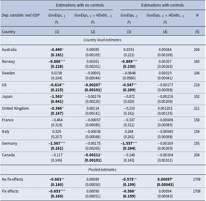
Note: This table shows our OLS estimates for $\beta _{1}$
and
$\beta _{1}$
and $\beta _{3}$
. Columns (1) and (2) display our estimates when we do not include control variables (real private consumption and interest rate) in the regression. Columns (3) and (4) show the estimations when we include our control variables. In column (5), N refers to the sample size. Estimations for
$\beta _{3}$
. Columns (1) and (2) display our estimates when we do not include control variables (real private consumption and interest rate) in the regression. Columns (3) and (4) show the estimations when we include our control variables. In column (5), N refers to the sample size. Estimations for $\beta _{3}$
measure the effect of one standard deviation in the interaction between government expenditures and household debt on Real GDP. Standard errors are clustered at the country level. Source: FRED data. Estimation sample for each country can be found in Table 2 in the appendix. Standard errors in parentheses. *p < 0.05, **p < 0.01, ***p < 0.001.
$\beta _{3}$
measure the effect of one standard deviation in the interaction between government expenditures and household debt on Real GDP. Standard errors are clustered at the country level. Source: FRED data. Estimation sample for each country can be found in Table 2 in the appendix. Standard errors in parentheses. *p < 0.05, **p < 0.01, ***p < 0.001.
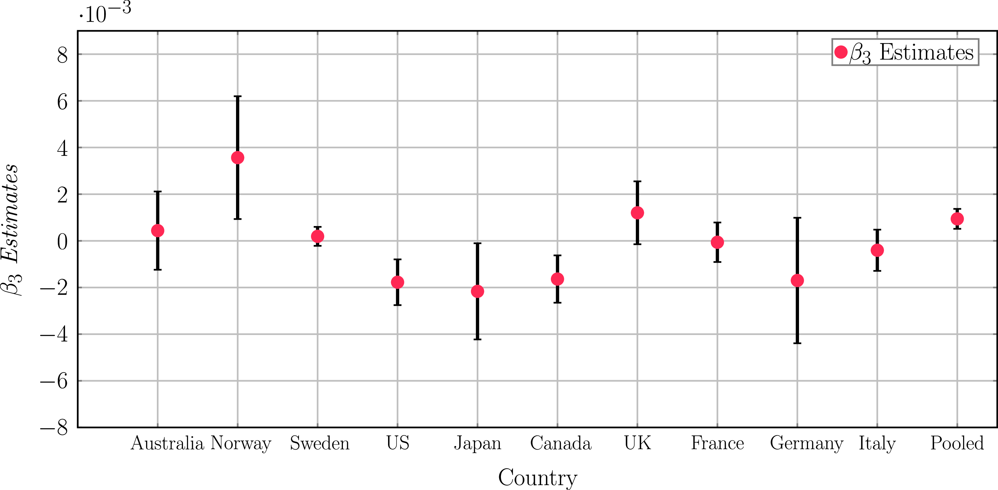
Our initial results are not conclusive about the presence of nonlinear effects of household debt on the estimation of the fiscal multiplier. As Fig. 2 shows the effect ( $\beta _{3}$
) is negative for some countries and positive for others. It is important to mention that our preliminary results are estimated through a linear model that studies the relationship between each variable and our dependent variable (Real Growth GDP), but it does not capture dynamic responses. For this reason, it is more appropriate to consider the analysis in an endogenous system like the one introduced in Section 3.
$\beta _{3}$
) is negative for some countries and positive for others. It is important to mention that our preliminary results are estimated through a linear model that studies the relationship between each variable and our dependent variable (Real Growth GDP), but it does not capture dynamic responses. For this reason, it is more appropriate to consider the analysis in an endogenous system like the one introduced in Section 3.
OLS estimations. Note: This figure shows our OLS estimates for $\beta _{3}$
. The upper and lower bound is plus and minus one standard deviation. Source: FRED data. Estimation sample for each country can be found in Table 2 in the appendix.
$\beta _{3}$
. The upper and lower bound is plus and minus one standard deviation. Source: FRED data. Estimation sample for each country can be found in Table 2 in the appendix.
3. Empirical model: STVAR and Bayesian inference
To identify whether the size of the fiscal multiplier changes between low or high-indebted states we use a STVAR as in Rothman et al. (Reference Rothman, Van Dijk and Hans2001), Gefang and Strachan (Reference Gefang and Strachan2009), and Gefang (Reference Gefang2012). The economic rationale for selecting this model is its ability to test the assumption that low and high levels of debt commitments condition households’ behavior differently after receiving a fiscal transfer. If correct, this would imply that the impact of fiscal expansions on economic activity is affected by differing levels of household debt.
The main reason we choose a smooth transition model, and not a Markov switching structure, as Markov Switching Vector Autoregresive, is that we intend to identify regime changes through a particular transition variable and avoid relying on a flexible evolution equation as Markov switching regime models do (Deschamps (Reference Deschamps2008)). Furthermore, in a model that uses macroeconomic data, such as GDP and government spending, it is our purpose to identify regime changes only triggered by changes in the level of household debt, and not by other variables of the system, such as GDP.
Another reason for not adopting a Markov switching model is that regime changes are exogenous, while in the smooth transition framework, regime changes are predetermined by the transition variable selected. Finally, Markov switching models are susceptible to experience abrupt changes in regimes. This is because the variable that identifies regimes is a discrete random variable with a value of zero in the first regime and a value of unity in the second. By contrast, smooth transition models rely on a logarithm function that allocates different weights to each regime while it nests a two-regime switching model as a special case. This model’s characteristic helps us to capture smooth movements of the economy along the business cycle.
The selection of our model also excludes time-varying parameter (TVP) models. This was motivated by the evidence that TVP models do not pick up the regime switches as well as smooth transition models (Koop and Potter (Reference Koop and Potter2010)). This may be explained by the fact that if TVP models have more shocks than observed variables, they cannot fully recover from economic shocks (Pagan and Robinson (Reference Pagan and Robinson2022)). Another reason for not considering TVP models is that they do not explain why coefficients are changing over time, and let the model drive it by itself. This characteristic does not allow us to identify the particular role of household debt in our system.
We follow Gefang and Strachan (Reference Gefang and Strachan2009) for describing the model. Although there is no formal definition of what is a low- and high-indebted state, the smooth transition function helps us to identify possible regime changes endogenously. We use a Bayesian estimation and generalized impulse response functions to measure the size of the fiscal multiplier.
This methodology identifies the equilibrium and presence of nonlinearity in our model in a single step. While classical estimation techniques often require multiple steps and Taylor expansions, this approach is less likely to have inaccurate approximation problems. An advantage of using an STVAR is that it allows to capturing smooth and discrete adjustments in the macroeconomic data.
3.1. The model
Our model specification follows Teräsvirta (Reference Teräsvirta1994) and Gefang and Strachan (Reference Gefang and Strachan2009). We examine the relationship between government expenditures and output within a nonlinear independent system, which includes output ( $y_{t}$
), government consumption expenditure (
$y_{t}$
), government consumption expenditure ( $g_{t}$
), private consumption (
$g_{t}$
), private consumption ( $c_{t}$
), credit household (
$c_{t}$
), credit household ( $h_{t}$
), and interest rate (
$h_{t}$
), and interest rate ( $r_{t}$
). We denominate
$r_{t}$
). We denominate $x_{t}=(y_{t},g_{t},c_{t},h_{t},r_{t})$
the model of the
$x_{t}=(y_{t},g_{t},c_{t},h_{t},r_{t})$
the model of the $1\ \times \ n$
(with
$1\ \times \ n$
(with $n=5$
) vector time series process
$n=5$
) vector time series process $x_{t}$
,
$x_{t}$
, $t=1,\ldots .,T$
conditioning on the
$t=1,\ldots .,T$
conditioning on the $p$
observations
$p$
observations $t=-p+1,\ldots,0$
.
$t=-p+1,\ldots,0$
.
We estimate the following equation:
 \begin{equation} x_{t}=\mu +\sum _{h=1}^{p}\varGamma _{h} x_{t-h}+F(z_{t})\left (\mu ^{z}+\sum _{h=1}^{p}\varGamma _{h}^{z} x_{t-h}\right )+\varepsilon _{t} \end{equation}
where $\varepsilon _{t}$
is a Gaussian white noise process with
$\varepsilon _{t}$
is a Gaussian white noise process with $E(\varepsilon _{t})=0,$ $ E(\varepsilon^{\prime}_{s}\varepsilon _{t})=\Sigma$
for
$ E(\varepsilon^{\prime}_{s}\varepsilon _{t})=\Sigma$
for $s=t$
, and
$s=t$
, and $E(\varepsilon^{\prime}_{s}\varepsilon _{t})=0$
for
$E(\varepsilon^{\prime}_{s}\varepsilon _{t})=0$
for $s\neq t$
.
$s\neq t$
. $\varGamma _{h}^{z}$
and
$\varGamma _{h}^{z}$
and $\varGamma _{h}$
describe how the process adjusts to changes in
$\varGamma _{h}$
describe how the process adjusts to changes in $ x_{t-h}$
and h identifies time horizon periods from today. The dimensions of
$ x_{t-h}$
and h identifies time horizon periods from today. The dimensions of $\varGamma _{h}$
and
$\varGamma _{h}$
and $\varGamma _{h}^{z}$
are
$\varGamma _{h}^{z}$
are $n\times n$
.
$n\times n$
. $\mu$
and
$\mu$
and $\mu ^{z}$
identify linear deterministic trends, which could be interpreted as the long-run behavior (steady states) of our variables (Villani (Reference Villani2009)). This specification allows us to separate beliefs about the deterministic trend component from beliefs about the persistence of fluctuations around this trend.
$\mu ^{z}$
identify linear deterministic trends, which could be interpreted as the long-run behavior (steady states) of our variables (Villani (Reference Villani2009)). This specification allows us to separate beliefs about the deterministic trend component from beliefs about the persistence of fluctuations around this trend.
Regime changes in the model are captured by a smooth transition function ( $F(z_{t})$
) introduced by Granger et al. (Reference Granger and Terasvirta1993) and Teräsvirta (Reference Teräsvirta1994) where
$F(z_{t})$
) introduced by Granger et al. (Reference Granger and Terasvirta1993) and Teräsvirta (Reference Teräsvirta1994) where $z_{t}$
is a transition continuous variable identifying the states. Note that
$z_{t}$
is a transition continuous variable identifying the states. Note that $z_{t}$
can be an exogenous variable or lagged endogenous variable of our model.
$z_{t}$
can be an exogenous variable or lagged endogenous variable of our model.
 \begin{equation} F(z_{t})=\{1+exp[{-}\gamma (z_{t}-c)/\sigma ]\}^{^{-1}} \end{equation}
The transition function $F(z_{t})$
is bounded by 0 and 1. The parameter gamma (which is non-negative) determines the speed of the smooth transition. We can see that when gamma tends to be infinite, the transition function becomes a Dirac function and the model becomes a two-state threshold VAR model. When gamma tends = 0, the transition function becomes a constant (equal to 0.5), and the nonlinear model turns into a linear VAR(
$F(z_{t})$
is bounded by 0 and 1. The parameter gamma (which is non-negative) determines the speed of the smooth transition. We can see that when gamma tends to be infinite, the transition function becomes a Dirac function and the model becomes a two-state threshold VAR model. When gamma tends = 0, the transition function becomes a constant (equal to 0.5), and the nonlinear model turns into a linear VAR( $p$
). The value of sigma could be reasonably set to 1. However, if we set this parameter equal to the standard deviation of the transition variable
$p$
). The value of sigma could be reasonably set to 1. However, if we set this parameter equal to the standard deviation of the transition variable $z_{t}$
, this normalizes gamma. We assume
$z_{t}$
, this normalizes gamma. We assume $\sigma =1$
. The parameter
$\sigma =1$
. The parameter $c$
is the point of inflection of the transition function whose value is uniformly distributed between the middle 50% values of the transition function. The transition between the two states is smooth and governed by the values of the parameters in the smooth function of
$c$
is the point of inflection of the transition function whose value is uniformly distributed between the middle 50% values of the transition function. The transition between the two states is smooth and governed by the values of the parameters in the smooth function of $z_{t}$
denoted by
$z_{t}$
denoted by $F(z_{t})$
. The value of
$F(z_{t})$
. The value of $F(z_{t})$
is bounded by 0 and 1 since
$F(z_{t})$
is bounded by 0 and 1 since $F(z_{t})$
= 0 when
$F(z_{t})$
= 0 when $z_{t}$
= -infinite, and
$z_{t}$
= -infinite, and $F(z_{t})$
= 1 when
$F(z_{t})$
= 1 when $z_{t}$
= infinite.
$z_{t}$
= infinite.
The transition between regimes is smooth for reasonable values of gamma ( $\gamma$
). The lower regime dynamic of the model (1) is determined by:
$\gamma$
). The lower regime dynamic of the model (1) is determined by:
 \begin{equation} x_{t}=\mu +\sum _{h=1}^{p} \varGamma _{h}x_{t-h}+\varepsilon _{t} \end{equation}
While in the upper regime, the model’s dynamics are determined by:
 \begin{equation} x_{t}=(\mu +\mu ^{z})+\sum _{h=1}^{p} \left(\varGamma _{h}+\varGamma _{h}^{z}\right)x_{t-h}+\varepsilon _{t} \end{equation}
In this model, the two regimes are associated with small and large values of the transition variable ( $z_{t}$
) relative to the point of inflection (
$z_{t}$
) relative to the point of inflection ( $c$
) of the transition function. Small values of
$c$
) of the transition function. Small values of $z_{t}$
are linked to the lower regime and large values of
$z_{t}$
are linked to the lower regime and large values of $z_{t}$
to the upper regime. For values of the transition variable below the point of inflection, the transition function (
$z_{t}$
to the upper regime. For values of the transition variable below the point of inflection, the transition function ( $F(z _{t})$
) will yield values below 0.5. On the other hand, for values of the transition variable above the point of inflection, the transition function will yield values above 0.5.
$F(z _{t})$
) will yield values below 0.5. On the other hand, for values of the transition variable above the point of inflection, the transition function will yield values above 0.5.
We take advantage of the transition function to identify low-debt and high-debt states. Given that there is no formal definition to recognize periods of low and high household debt, we employ criteria based on the probability of transitioning between regimes. We identify periods of low and high debt if the probability of transitioning is respectively below or above 0.5. In other words, we classify periods of low and high debt as the value of the transition variable is below or above a cutoff parameter estimated by the model. Because the cutoff parameter plays a key role in identifying regimes, we conduct robustness checks for our identification strategy.
The specification of our model allows us to adopt exogenous or lagged endogenous variables to trigger regime changes. Our research question involves identifying regimes of periods of low and high household debt. To do that we examine two time series: credit to nonfinancial sector-to-GDP ratio, as in Bernardini and Peersman (Reference Bernardini and Peersman2018), and residential housing prices. Note that our decision to include housing prices in the transition function was influenced by the findings of Terrones et al. (Reference Terrones, Claessens and Kose2011), which reveal a strong synchronization between housing prices and levels of household debt during financial cycles. Due to this synchronization, housing prices serve as a valuable proxy or indicator for identifying periods of low and high household debt.
To examine which time series plays a better role in triggering regime changes, we consider the first difference in year-to-year and quarter-to-quarter variations for each time series.
- $(f=1)z_{t}=\triangle ^{y/y}{p_{t-1}}$
, residential housing prices growth - year-to-year variation
$(f=1)z_{t}=\triangle ^{y/y}{p_{t-1}}$
, residential housing prices growth - year-to-year variation -
$(f=2)z_{t}=\triangle ^{y/y}{h_{t-1}}$
, household debt to GDP - year-to-year variation
-
$(f=3)z_{t}=\triangle ^{q/q}{p_{t-1}}$
, residential housing prices growth - quarter-to-quarter variation
-
$(f=4)z_{t}=\triangle ^{q/q}h_{t-1}$
, household debt to GDP - quarter-to-quarter variation


3.2. Bayesian inference
Our Bayesian estimation incorporates the collapse Gibbs sampler as in Koop et al. (Reference Koop, León-González and Strachan2009). In comparison to the standard Gibbs sampler, or block Gibbs sampler, this algorithm has the special feature that computes as many marginal probabilities as possible before sampling the conditional probability, which helps to speed up the convergence (see the appendix for a detailed description of the algorithm).
Priors.
The selection of priors is crucial to avoid in-sample overfitting and poor out-of-sample forecasting accuracy (Giannone et al. (Reference Giannone, Lenza and Primiceri2019)). Following Villani (Reference Villani2009), we adopt prior information on the steady-state variables of the system. This approach lets economic theory play a central role in the elicitation of our priors. We also follow Gefang and Strachan (Reference Gefang and Strachan2009) and Gefang (Reference Gefang2012) for the prior selection of transition functions between regimes.
For $\gamma$
, the smooth transition parameter, we assume Gamma(1,0.001) to let the data dominate the prior for
$\gamma$
, the smooth transition parameter, we assume Gamma(1,0.001) to let the data dominate the prior for $\gamma$
. This is because it is difficult to impose meaningful informative priors for both the parameters that indicate the transition of regimes. Using Gamma distribution, we exclude a priori the point
$\gamma$
. This is because it is difficult to impose meaningful informative priors for both the parameters that indicate the transition of regimes. Using Gamma distribution, we exclude a priori the point $\gamma =0$
from the integration range and thus, we avoid non-identification problems. The prior for
$\gamma =0$
from the integration range and thus, we avoid non-identification problems. The prior for $c$
, the point inflection parameter, is assumed uniformly distributed between the middle 50% ranges of the transition variables.
$c$
, the point inflection parameter, is assumed uniformly distributed between the middle 50% ranges of the transition variables.
The variance-covariance matrix of error terms of the vectorization model is represented by $\Sigma$
. Following Zellner (Reference Zellner1971), we set a standard diffuse prior for
$\Sigma$
. Following Zellner (Reference Zellner1971), we set a standard diffuse prior for $\Sigma$
.
$\Sigma$
.
 \begin{align*} p(\Sigma ) \,=\, \propto |\Sigma |^{-(n+1)/2} \end{align*}
As in the vectorized model described in the appendix, $b$
identifies the vectorization of
$b$
identifies the vectorization of $\varGamma$
for each regime. Following Strachan and van Dijk (Reference Strachan and van Dijk2006), we set a weakly informative conditional proper prior for
$\varGamma$
for each regime. Following Strachan and van Dijk (Reference Strachan and van Dijk2006), we set a weakly informative conditional proper prior for $b$
to have well-defined posterior probabilities.
$b$
to have well-defined posterior probabilities.
 \begin{align*} p\left(b|\Sigma,\gamma,c,\mu,M_{\omega }\right) \,=\, \propto N\left(0,\eta ^{-1}I_{k}\right), \end{align*}
where $k=2(2+n\times p)$
,
$k=2(2+n\times p)$
, $\eta$
is the shrinkage parameter, and
$\eta$
is the shrinkage parameter, and $M_{\omega }$
identifies our data. For
$M_{\omega }$
identifies our data. For $\mu$
, the steady-state means of our variables, we set a prior of the form
$\mu$
, the steady-state means of our variables, we set a prior of the form $p(\mu )$
=
$p(\mu )$
= $\propto N(\mu _{0},\Sigma _{\mu })$
.
$\propto N(\mu _{0},\Sigma _{\mu })$
.
Furthermore, our prior selection for the smooth transition of the model becomes relevant to tackle the non-identification problem that arises when $\gamma =0$
. The selection of our prior distribution eliminates the point
$\gamma =0$
. The selection of our prior distribution eliminates the point $\gamma =0$
.
$\gamma =0$
.
Our prior for the variance-covariance matrix is an inverse Wishart distribution, commonly used in Bayesian analysis due to its conjugacy properties with the normal sampling model (Alvarez et al. (Reference Alvarez, Niemi and Simpson2014), Liu et al. (Reference Liu, Zhang and Grimm2016), Zhang (Reference Zhang2021)). By choosing this prior distribution, the posterior distribution is also an inverse Wishart distribution given normally distributed data. As Zhang (Reference Zhang2021) shows, the posterior mean can be obtained by averaging the sample covariance matrix over the prior mean.
Finally, the selection of the uniform distribution as a prior for the point of inflection ( $c$
) follows Gefang (Reference Gefang2012). However, we should mention this prior may be chosen in many ways. Table 2 summarizes our priors.
$c$
) follows Gefang (Reference Gefang2012). However, we should mention this prior may be chosen in many ways. Table 2 summarizes our priors.
Priors
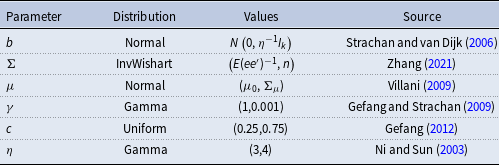
Note: This table shows the sources we use for the selection of priors.
Generalized Impulse Response Functions.
Following Koop et al. (Reference Koop, Pesaran and Potter1996), we use a generalized impulse response function (GIRF) to examine output responses to a government expenditure shock. The GIRF simulates the future path of the economy with and without a structural shock and captures the responses when the threshold variable is allowed to respond endogenously. We introduce a shock whose magnitudes account for $+1$
time the standard deviation of the quarterly government expenditure growth rates. Unlike traditional impulse responses (OIRFs), generalized impulse response functions do not require orthogonal errors, and therefore, they have the advantage of being unique. This means that they are able to shock only one element of the covariance matrix, and thus, they are invariant to the ordering of the variables in
$+1$
time the standard deviation of the quarterly government expenditure growth rates. Unlike traditional impulse responses (OIRFs), generalized impulse response functions do not require orthogonal errors, and therefore, they have the advantage of being unique. This means that they are able to shock only one element of the covariance matrix, and thus, they are invariant to the ordering of the variables in $x_{t}$
(Koop et al. (Reference Koop, Pesaran and Potter1996), Pesaran and Shin (Reference Pesaran and Shin1998)). More details can be found in the appendix.
$x_{t}$
(Koop et al. (Reference Koop, Pesaran and Potter1996), Pesaran and Shin (Reference Pesaran and Shin1998)). More details can be found in the appendix.
We use Bayesian Model Averaging to calculate the generalized impulse response functions. This method consists of averaging parameter uncertainties, model uncertainties, history uncertainties, and future uncertainties by the weighted probability of each model. As in Koop et al. (Reference Koop, Pesaran and Potter1996) and Fazzari et al. (Reference Fazzari, Morley and Panovska2015), we construct the (1 - $\alpha$
)
$\alpha$
) $ *$
100% credibility bounds ordering the impulse responses whose posterior likelihood was in the upper (1 -
$ *$
100% credibility bounds ordering the impulse responses whose posterior likelihood was in the upper (1 - $\alpha$
)
$\alpha$
) $*$
100 percentile. As Fazzari et al. (Reference Fazzari, Morley and Panovska2015) state, this methodology leads us to build a credibility cloud of generalized impulsed response functions. We report bounds at 5 and 95% of credibility.
$*$
100 percentile. As Fazzari et al. (Reference Fazzari, Morley and Panovska2015) state, this methodology leads us to build a credibility cloud of generalized impulsed response functions. We report bounds at 5 and 95% of credibility.
We use fiscal multipliers to study whether the effects of government spending differ across regimes. We set the magnitude of the government spending multiplier as the percentage change in real GDP caused by a one percent increase in a fiscal variable. We compute the cumulative fiscal multiplier defined as
 \begin{equation} Multiplier_{h}=\frac{\sum _{j=1}^{h}y_{j}}{\sum _{j=1}^{h}g_{j}}\times \frac{1}{\sigma _{g}} \end{equation}
where $y_{j}$
and
$y_{j}$
and $g_{j}$
are output and government spending response parameters of period
$g_{j}$
are output and government spending response parameters of period $j$
.
$j$
. $\sigma _{g}$
represents the standard deviation of government expenditures that we include to normalize the fiscal expenditure shock to one percent.
$\sigma _{g}$
represents the standard deviation of government expenditures that we include to normalize the fiscal expenditure shock to one percent.
It is worth noting that our definition of fiscal multiplier is more closely aligned with the concept of elasticity rather than the definition provided by Ramey and Zubairy (Reference Ramey and Zubairy2018) and Caldara and Kamps (Reference Caldara and Kamps2017). While these authors define fiscal multiplier as [“…dollar increase in output to an effective change in the fiscal variable of 1 dollar ”]…, we define it as the ratio of the change in output ( $\Delta Y$
) to a discretionary change in government spending (
$\Delta Y$
) to a discretionary change in government spending ( $\Delta G$
). Because our primary goal is to explore differences in output responses to a government spending shock during periods of low and high household debt, we have adopted the same definition as in Fazzari et al. (Reference Fazzari, Morley and Panovska2015), Spilimbergo et al. (Reference Spilimbergo, Schindler and Symansky2009).
$\Delta G$
). Because our primary goal is to explore differences in output responses to a government spending shock during periods of low and high household debt, we have adopted the same definition as in Fazzari et al. (Reference Fazzari, Morley and Panovska2015), Spilimbergo et al. (Reference Spilimbergo, Schindler and Symansky2009).
In our benchmark estimation, we choose an autoregressive order $p$
equal to six in each regime to capture long-term dynamics. The collapsed Gibbs sampler runs for 20,000 passes. We discard the first 2000. The time horizon (
$p$
equal to six in each regime to capture long-term dynamics. The collapsed Gibbs sampler runs for 20,000 passes. We discard the first 2000. The time horizon ( $h$
) of the impulse responses is 50 quarters (12.5 years), a medium-long span of a business cycle.
$h$
) of the impulse responses is 50 quarters (12.5 years), a medium-long span of a business cycle.
4. Empirical results
4.1. Data
We use quarterly data for the United States, United Kingdom, Canada, Germany, Italy, France, Japan, Australia, Norway, and Sweden. The data is obtained from the database of the Federal Reserve of St. Louis, the Bank for International Settlements, the Australia Bureau of Statistics, Norway Statistics, and Sweden Statistics.
For gross domestic product ( $y_{t}$
), real government final consumption expenditure (
$y_{t}$
), real government final consumption expenditure ( $g_{t}$
), and real private consumption (
$g_{t}$
), and real private consumption ( $c_{t}$
) we use seasonally adjusted data to remove yearly pattern effects. Data for credit to household sector-to-GDP ratios (
$c_{t}$
) we use seasonally adjusted data to remove yearly pattern effects. Data for credit to household sector-to-GDP ratios ( $h_{t}$
) and residential housing price index (
$h_{t}$
) and residential housing price index ( $p_{t}$
) is non-seasonally adjusted. For interest rates (
$p_{t}$
) is non-seasonally adjusted. For interest rates ( $i_{t}$
), we use the three-month interbank rate. All variables are expressed in logarithms except for interest rates which are expressed in percentages. Table 2 in the appendix shows the data period sample for each country.
$i_{t}$
), we use the three-month interbank rate. All variables are expressed in logarithms except for interest rates which are expressed in percentages. Table 2 in the appendix shows the data period sample for each country.
4.2. Models comparison
We analyze the model comparison results using Bayesian posterior probabilities and the ability of the transition function to identify low and high regimes. Figs. 1, 2, 3, and 4 in the appendix display transition functions when using household debt to GDP and housing prices for identifying regime changes.
We use posterior probabilities, calculated from the Bayes factors, to examine which transition variable plays a more important role in triggering regime changes. Assuming all our models are mutually independent and exhaustive, we allocate the same prior weight to each of them. Table 3 in the appendix presents each model’s probability.
Our posterior probabilities imply that using housing prices in the transition function accounts for a higher percentage of the posterior mass for Australia, Sweden, Norway, the United States, Italy, and Japan, while household debt to GDP accounts for a higher percentage of the posterior mass for the United Kingdom, Canada, Germany, and France.
However, a higher Bayes factor does not necessarily imply that the model identifies low and high regimes. For this reason, we also explore whether the transition function distribution is able to distinguish between low and high regimes for different values of the transition variable. This is a crucial step in the selection of the transition variable because not all transition functions are monotonically increasing probability functions. This implies that the probability of moving from a low to a high-debt regime is always increasing on the transition variable selected. In other words, the higher the household debt or the house price change is, the more likely the economy moves to a high-debt state in our model. Furthermore, the probability of identifying distinct regimes does not necessarily hinge on the size of the data sample, but primarily on the second moment of the transition variable. The standard deviation informs about the reliability of identifying low and high regimes at each value of the transition variable. To examine the monotonic increasing property, we analyze the transition function distributions displayed in Figs. 3 and 4.
Transition function and high debt state probability for Australia, Sweden, and Norway. Note: This figure displays the transition function and the probability of transitioning to a high-debt state for Australia, Sweden, and Norway. In the left column, the transition functions (dashed line $ -$
left y-axis) alongside the data employed to construct them (solid line
$ -$
left y-axis) alongside the data employed to construct them (solid line $ -$
right y-axis) can be observed. The right column illustrates the probability of transitioning to a high-debt state, with shaded areas indicating standard deviations.
$ -$
right y-axis) can be observed. The right column illustrates the probability of transitioning to a high-debt state, with shaded areas indicating standard deviations.

Transition function and high debt state probability for G7 countries. Note: This figure displays the transition function and the probability of transitioning to a high -debt state for G7 countries. In the left column, the transition functions (dashed line $ -$
left y-axis) alongside the data employed to construct them (solid line
$ -$
left y-axis) alongside the data employed to construct them (solid line $ -$
right y-axis) can be observed. The right column illustrates the probability of transitioning to a high-debt state, with shaded areas indicating standard deviations.
$ -$
right y-axis) can be observed. The right column illustrates the probability of transitioning to a high-debt state, with shaded areas indicating standard deviations.

Fig. 3 displays the selected transition functions for Australia, Sweden, and Norway. It is important to note that following our posterior probabilities we use year-to-year variation in housing prices as a transition variable for Norway.Footnote 1 It can be observed that transition probability functions are monotonically increasing in the transition variables. However, the speed of transitioning from a low to a high-debt regime differs among countries.
Fig. 4 depicts the selected transition functions for G7 countries. It is worth mentioning that our posterior probabilities results led us to use year-to-year variation in housing prices as a transition variable for Italy and Japan, and quarter-to-quarter variation in housing prices as a transition variable for France. Even when we consider using household debt to GDP as a transition function, we find that the transition probability distributions are not monotonically increasing in household debt. $^{1}$
It can be observed that the transition function for Canada fluctuates between zero and one, and it does not identify probabilities close to zero or one among the range of the household debt variation year-to-year. It is important to highlight that the less informative the transition function is, the more difficult it is to identify low- and high-debt regimes. The wide standard deviation in the transition probability function provides evidence of the regime identification challenge.
$^{1}$
It can be observed that the transition function for Canada fluctuates between zero and one, and it does not identify probabilities close to zero or one among the range of the household debt variation year-to-year. It is important to highlight that the less informative the transition function is, the more difficult it is to identify low- and high-debt regimes. The wide standard deviation in the transition probability function provides evidence of the regime identification challenge.
For Italy, France, Japan, and the United Kingdom, although the transition probability remains either at zero or one, changes in the transition variable need to be large to identify high probabilities of switching regimes. Because these changes are less likely to be observed in the sample, our model does not play a good role in identifying low and high regimes. Similarly, in the case of Italy and France, the wide standard deviations in the transition probability functions constitute evidence of the regime identification challenge.
Finally, we work with Australia, Sweden, Norway, the United States, and Germany. However, we raise concerns about countries, such as Germany, whose transition probability function fluctuates between 0.1 and 0.4 in the low state, and between 0.5 and 0.8 in the high state. This directly affects the standard deviation of the transition function, and may add some challenges to the regime identification.
4.3. Output responses to a government spending shock
We calculate the output responses to a government spending shock as explained in Section 3.2. We study the dynamic adjustment paths for government spending in Australia, Sweden, Norway, the United States, and Germany. Fig. 5 shows mean output responses to a government spending shock when we use lag $p=6$
.
$p=6$
.
GIRFs: Government spending multipliers
Notes: Fiscal multipliers represent the percent change of GDP after increasing government expenditures by 1%. Standard deviation in brackets. Lag $ p=6$
. Estimation sample for each country can be found in Table 2 in the appendix.
$ p=6$
. Estimation sample for each country can be found in Table 2 in the appendix.
GIRFs: Government spending multiplier. Note: This figure presents government spending multiplier for our sample economies. We calculate these figures following the definition of fiscal multiplier presented in equation (6). Mean responses (solid) and 95% credibility bands (shaded areas). Lag $p = 6$
. Estimation sample for each country can be found in Table 2 in the appendix.
$p = 6$
. Estimation sample for each country can be found in Table 2 in the appendix.

Our results imply that output responses, on impact ( $h=1$
), are higher when the fiscal expansion takes place during periods of low household debt. Furthermore, we find that the effect of government spending on output is more persistent when an increase in government spending occurs during periods of low household debt. Nevertheless, it is important to highlight that the dynamic of the persistence relies on how well the states are identified and the lag chosen in the model. Figs. 10 and 11 in the appendix display output responses when we modify the lag of the model to
$h=1$
), are higher when the fiscal expansion takes place during periods of low household debt. Furthermore, we find that the effect of government spending on output is more persistent when an increase in government spending occurs during periods of low household debt. Nevertheless, it is important to highlight that the dynamic of the persistence relies on how well the states are identified and the lag chosen in the model. Figs. 10 and 11 in the appendix display output responses when we modify the lag of the model to $p=4$
and
$p=4$
and $p=5$
.
$p=5$
.
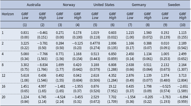
Our findings indicate that during periods of low household debt, an increase in government spending boosts the economy more than in periods of high household debt. This is the case in Australia, Norway, and the United States. Table 3 presents these results.
In Australia, an increase in government spending pushes output up in both regimes. However, this effect has an immediate effect only in low-debt states. During periods of low household debt, output increases from 0.83 to a cumulative change of 5.08 (percent of GDP) after 12 quarters, while during periods of high household debt, output increases from -0.46 to 0.44 (percent of GDP) after 12 periods. Our estimations show that the cumulative output response is higher in the low regime than in the high regime after 12 quarters. Our results for Australia also suggest that household debt may influence the output response on impact. This may be explained by households’ liquidity constraints as Eggertsson and Krugman (Reference Eggertsson and Krugman2012) and Galí et al. (Reference Galí, López-Salido and Vallés2007) claim.
Our evidence for Norway indicates that output increases by 0.27 (percent of GDP), on impact, during periods of low household debt, followed by a peak of 1.96 during the second year (seventh quarter). During periods of high household debt, we find that output increases 0.18 (percent of GDP) in the initial period, followed by a peak of 1.24 during the second year (fifth quarter). Our evidence is consistent with Boug et al. (Reference Boug, Cappelen and Eika2017) who found a government spending multiplier between 0.9 and 1.1 (percent of GDP) for Norway in the short and medium term using an input-output-based model.
In the case of the United States, we find that during periods of low household debt output increases from 1.019 to a cumulative change of 2.61 (percent of GDP) after 12 quarters, while during periods of high household debt, output increases from 0.60 to 4.35 (percent of GDP) after 12 periods. Contrary to Bernardini and Peersman (Reference Bernardini and Peersman2018), our evidence does not allow us to support the idea that fiscal spending multipliers are particularly high during periods of high private debt when we use lag $p=6$
. Nevertheless, our conclusions are similar to Bernardini and Peersman (Reference Bernardini and Peersman2018) when we estimate the model using lag
$p=6$
. Nevertheless, our conclusions are similar to Bernardini and Peersman (Reference Bernardini and Peersman2018) when we estimate the model using lag $p=4$
and lag
$p=4$
and lag $p=5$
.
$p=5$
.
For Germany and Sweden, we find larger fiscal multipliers on impact during periods of high household debt. After an expansion of government spending, output increases 1.22 and 0.19 (percent of GDP) (on impact) during periods of low household debt, and 1.56 and 1.11 (percent of GDP) during periods of high household debt in Germany and Sweden.
To sum up, our results show that on average the fiscal multiplier (on impact) is 1.29, 0.09, and 0.42 (percent of GDP) larger in low-debt states for Australia, Norway, and the United States. On the contrary, the multiplier is 0.35 and 0.92 (percent of GDP) larger when the fiscal expansion takes place during periods of high household debt.
This difference changes depending on the number of lags ( $p$
) incorporated into the model and the time horizon chosen for measuring the fiscal multiplier. For instance, the positive gap between the average fiscal multiplier, after 12 quarters, in periods of low and high debt remains positive for Australia and Norway, but not for the United States. It is worth mentioning that the longer the horizon to measure the fiscal multiplier is, the more dependent the model is on the identification of the states of the economy.
$p$
) incorporated into the model and the time horizon chosen for measuring the fiscal multiplier. For instance, the positive gap between the average fiscal multiplier, after 12 quarters, in periods of low and high debt remains positive for Australia and Norway, but not for the United States. It is worth mentioning that the longer the horizon to measure the fiscal multiplier is, the more dependent the model is on the identification of the states of the economy.
4.4. Robustness
In this section, we study the robustness of our model. Particularly, we study the behavior of the transition function probability to changes in the point of inflection ( $ c$
) and the smooth transition parameter (
$ c$
) and the smooth transition parameter ( $\gamma$
). We also study how sensitive our baseline results are to changes in the identification strategy and the selection of lags. As we mentioned above, the likelihood of identifying different regimes does not necessarily depend on the size of the data sample, but mostly on the second moment of the variable chosen for the transition.
$\gamma$
). We also study how sensitive our baseline results are to changes in the identification strategy and the selection of lags. As we mentioned above, the likelihood of identifying different regimes does not necessarily depend on the size of the data sample, but mostly on the second moment of the variable chosen for the transition.
4.4.1. The role of the transition function
State-dependent models deal with the challenge of identifying different states. In our case, we aim to identify low and high periods of household debt using a transition probability function which, in our model, depends on two main parameters: the point of inflection ( $c$
) and the smooth transition parameter (
$c$
) and the smooth transition parameter ( $\gamma$
).
$\gamma$
).
The point of inflection parameter.
The point of inflection ( $c$
) governs the identification of low and high regimes. For values of the transition variable below the
$c$
) governs the identification of low and high regimes. For values of the transition variable below the $c$
parameter, the model yields a probability below 0.5. Contrary, for values of the transition variable above the point of inflection, the model yields a probability above 0.5.
$c$
parameter, the model yields a probability below 0.5. Contrary, for values of the transition variable above the point of inflection, the model yields a probability above 0.5.
We modify the estimation of the point of inflection of the transition function. In our benchmark model, the value of $c$
is uniformly distributed between the middle 50% values of the transition variable. Now, we reestimate the value of
$c$
is uniformly distributed between the middle 50% values of the transition variable. Now, we reestimate the value of $c$
from a uniform distribution between the middle 60% of the values. Fig. 8 in the appendix displays the average transition probability function and its standard deviation for each country of analysis. In general, enlarging the sample of values to reestimate the point of inflection parameter increases the standard deviation of the transition probability function, attributed to the sample dispersion of the selected transition variable. Thus, it adds more challenges to identify changes between regimes at different values of the transition variables.
$c$
from a uniform distribution between the middle 60% of the values. Fig. 8 in the appendix displays the average transition probability function and its standard deviation for each country of analysis. In general, enlarging the sample of values to reestimate the point of inflection parameter increases the standard deviation of the transition probability function, attributed to the sample dispersion of the selected transition variable. Thus, it adds more challenges to identify changes between regimes at different values of the transition variables.
The gamma (smooth transition) parameter.
The gamma parameter ( $ \gamma$
) determines the speed of smooth transition between low-debt and high-debt states. We study how sensitive the transition probability function is when the smooth transition parameter changes. Recall that the smooth transition parameter is estimated through a gamma distribution function with shape and scale parameters defined in our benchmark model. We modify the shape parameter in the gamma distribution function from 10 to 9. Fig. 9 in the appendix shows the transition probability functions before and after the change. In general, the standard deviation of the transition probability function is sensitive to changes, whereas the average transition probability function (dashed line) is less affected with respect to the benchmark model. For instance, the average transition probability function does not change significantly after changing the shape parameter in the gamma distribution function for Norway and the United States, but it changes notoriously for Germany, France, Italy, and the United Kingdom.
$ \gamma$
) determines the speed of smooth transition between low-debt and high-debt states. We study how sensitive the transition probability function is when the smooth transition parameter changes. Recall that the smooth transition parameter is estimated through a gamma distribution function with shape and scale parameters defined in our benchmark model. We modify the shape parameter in the gamma distribution function from 10 to 9. Fig. 9 in the appendix shows the transition probability functions before and after the change. In general, the standard deviation of the transition probability function is sensitive to changes, whereas the average transition probability function (dashed line) is less affected with respect to the benchmark model. For instance, the average transition probability function does not change significantly after changing the shape parameter in the gamma distribution function for Norway and the United States, but it changes notoriously for Germany, France, Italy, and the United Kingdom.
GIRFs: Fiscal multipliers. A comparison between thresholds. Note: This figure presents government spending multiplier for Australia, Norway, United States, and Germany using different thresholds to identify low and high household debt states. We calculate these figures following the definition of fiscal multiplier presented in equation (6). Mean responses (solid) and 95 % credibility bands (shaded areas). Estimation sample for each country can be found in Table 2 in the appendix.

Figs. 6 and 7 in the appendix display the posterior probabilities for the point of inflation ( $c$
), the speed of transition (
$c$
), the speed of transition ( $\gamma$
), the shrinkage parameter for lag estimates, and the steady-state (
$\gamma$
), the shrinkage parameter for lag estimates, and the steady-state ( $\mu$
) parameters estimated for Australia, Sweden, Norway, the United States, and Germany. Our results show that, while the posterior probabilities for the
$\mu$
) parameters estimated for Australia, Sweden, Norway, the United States, and Germany. Our results show that, while the posterior probabilities for the $\gamma$
parameter are similar across countries, there are differences in the posterior probabilities for the
$\gamma$
parameter are similar across countries, there are differences in the posterior probabilities for the $c$
parameter. These differences are attributed to the range and dispersion of the transition variable used to estimate the
$c$
parameter. These differences are attributed to the range and dispersion of the transition variable used to estimate the $c$
parameter. Our findings also suggest disparities in the steady-state variable that identifies the linear trend for household debt across countries.
$c$
parameter. Our findings also suggest disparities in the steady-state variable that identifies the linear trend for household debt across countries.
4.4.2. Changing the identification strategy
We reestimate our model’s results after changing the identification of low and high household debt states. Initially, we define an economy to be in a high-debt state if the probability of transitioning ( ${F}(z_{t})$
) is above 0.5 and in a low-debt state if the probability of transitioning is below 0.5. Because the 0.5 threshold is arbitrarily selected, we now define an economy to be in a high regime if the probability of transitioning is above 0.6 and in a low regime if the probability of transitioning is below 0.4. In other words, our new identification strategy requires a higher likelihood to identify low- and high-debt states. Fig. 6 shows output responses in low and high-debt states under our new identification strategies for Australia, Sweden, Norway, the United States, and Germany.
${F}(z_{t})$
) is above 0.5 and in a low-debt state if the probability of transitioning is below 0.5. Because the 0.5 threshold is arbitrarily selected, we now define an economy to be in a high regime if the probability of transitioning is above 0.6 and in a low regime if the probability of transitioning is below 0.4. In other words, our new identification strategy requires a higher likelihood to identify low- and high-debt states. Fig. 6 shows output responses in low and high-debt states under our new identification strategies for Australia, Sweden, Norway, the United States, and Germany.
In general, our results suggest that changing the identification strategy does not affect fiscal multipliers (on impact) during periods of low household debt, but it affects our estimations for periods of high household debt. This constitutes evidence of the sensitivity of the identification assumption on the high regime.
Fig. 6 also informs about the dynamic of output responses. It shows that for horizons greater than zero, output responses are conditioned by the challenges in identifying regimes. It can be seen that reducing the threshold to identify the low-debt state increases the output response after the tenth quarter for Australia and Sweden and increases the output response standard deviation for Norway. On the other hand, an increase in the threshold to identify the high-debt state increases the output response for Australia and reduces the output response for Sweden. The latter implies that the more likely the economy to be in a high-debt state, the lower the output response to fiscal stimulus is.
4.4.3. The role of lags
We also analyze the effect of lags on our results. To do that, we compare the fiscal multiplier on impact, and after four and eight quarters when we specify a model with lag p = 6, p = 5, and p = 4. It is important to highlight that the model’s estimations after four and eight quarters are conditioned by the identification of the low and high regimes. For this reason, we believe is more informative to focus on the fiscal multiplier on impact. Table 4 presents our estimations.
Fiscal multipliers: The role of lags
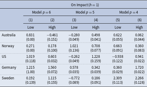
Notes: This table shows fiscal multipliers (on impact, $h=1$
) for a model with lag
$h=1$
) for a model with lag $p=6$
,
$p=6$
, $p=5$
, and
$p=5$
, and $p=4$
. Fiscal multipliers represent the percent change of GDP after increasing government expenditures by 1%. Standard deviation in brackets. Estimation sample for each country can be found in Table 2 in the appendix.
$p=4$
. Fiscal multipliers represent the percent change of GDP after increasing government expenditures by 1%. Standard deviation in brackets. Estimation sample for each country can be found in Table 2 in the appendix.
When we analyze the fiscal multiplier on impact (columns (1) to (6)), we observe that changing the model’s lag to p = 5 affects our conclusions for Australia, the United States, and Germany. Now, output responses are higher when the fiscal expansion takes place during periods of high household debt in Australia and the United States. For Germany, our results suggest that the fiscal multiplier is larger during periods of low household debt. It is worth noting that the precision of our estimates also changes depending on the country and the state of the economy.
When we consider a model’s lag equal to p = 4, our conclusions remain the same as in the benchmark model (p = 6) for Australia, Norway, and Germany. We should also note that our estimates for the low state increase compared to the results of our benchmark model for Norway. In Table 6, in the appendix, we extend the analysis when we consider the fiscal multiplier after four and eight quarters.
Finally, it is important to mention that comparing the model results at different lags suggests how sensitive estimates are to the chosen time horizon of the model.
5. A model comparison: STVAR vs. state-dependent local projections
Because the STVAR and STVAR with robustness models use the same transition function for identifying low and high regimes, our model comparison does not avoid identification concerns. For this reason, we compare our model results with estimations from a SD-LP model. Local Projection (LP) estimations are well-known for having smaller bias, but at the cost of higher variance (Plagborg-Møller and Wolf (Reference Plagborg-Møller and Wolf2021)). We use this methodology with the special purpose of comparing the LP and STVAR estimations on impact. Our decision to use an SD-LP methodology is based on the fact that this model is also able to identify low and high states endogenously. As in the STVAR model, the dynamic of the impulse response functions in the LP setting also relies on the identification of regimes. It is important to note that while the STVAR model computes generalized impulse response functions, the SD-LP model uses orthogonalized impulse response functions.Footnote 2
Our state-dependent local projection model specification follows Jordà (Reference Jordà2005) and Alloza (Reference Alloza2022).
 \begin{align} x_{t+h} & = F(z_{t-1})\left[\alpha _{A,h}+\psi _{A,h}(L)x_{t-1}+\beta _{A,h}shock_{t}^{G}\right]+ \nonumber\\ &\quad +\left[1-F(z_{t-1})\right]\left[\alpha _{B,h}+\psi _{B,h}(L)x_{t-1}+\beta _{B,h}shock_{t}^{G}\right]+\varepsilon _{t+h} \end{align}
 \begin{equation} F_{z_{t}}=\frac{exp({-}\gamma z_{t})}{1+exp({-}\gamma z_{t})} \end{equation}
where $x_{t}=(y_{t},g_{t},c_{t},h_{t},r_{t})$
is a vector of output (
$x_{t}=(y_{t},g_{t},c_{t},h_{t},r_{t})$
is a vector of output ( $y_{t}$
), government consumption expenditure (
$y_{t}$
), government consumption expenditure ( $g_{t}$
), private consumption (
$g_{t}$
), private consumption ( $c_{t}$
), credit household (
$c_{t}$
), credit household ( $h_{t}$
), and interest rate (
$h_{t}$
), and interest rate ( $r_{t}$
).
$r_{t}$
). $shock_{t}^{G}$
is an exogenous government spending shock.
$shock_{t}^{G}$
is an exogenous government spending shock. $\psi _{A,h}(L)$
and
$\psi _{A,h}(L)$
and $\psi _{B,h}(L)$
are polynomials in the lag operator of order six for regime
$\psi _{B,h}(L)$
are polynomials in the lag operator of order six for regime $A$
(low-debt regime) and
$A$
(low-debt regime) and $B$
(high-debt regime). For each regression
$B$
(high-debt regime). For each regression $h$
, the coefficient
$h$
, the coefficient $\beta _{A,h}$
measures the response of the variable
$\beta _{A,h}$
measures the response of the variable $x_{t}$
to a government spending shock
$x_{t}$
to a government spending shock $shock_{t}^{G}$
during state
$shock_{t}^{G}$
during state $A$
and, conversely,
$A$
and, conversely, $\beta _{B,h}$
captures the response during state
$\beta _{B,h}$
captures the response during state $B$
.
$B$
. $\alpha _{A,h}$
and
$\alpha _{A,h}$
and $\alpha _{B,h}$
are time-varying intercepts that help us to avoid the possibility that coefficients
$\alpha _{B,h}$
are time-varying intercepts that help us to avoid the possibility that coefficients $\beta _{A,h}$
or
$\beta _{A,h}$
or $\beta _{B,h}$
reflect the impact of a regime instead of the government spending shock. For each country, we use the same transition variables (
$\beta _{B,h}$
reflect the impact of a regime instead of the government spending shock. For each country, we use the same transition variables ( $z_{t}$
) as in the STVAR model.
$z_{t}$
) as in the STVAR model.
Although state-dependent local projection models are computationally less challenging to estimate rather than STVAR models, it is important to highlight under which conditions they work. As Gonçalves et al. (Reference Gonçalves, Herrera, Kilian and Pesavento2022) state, the validity of the LP estimator depends on the information used to identify the states, which in our case is part of the endogenous variables of the model. If the identification of the states depends on endogenous variables, the estimator [“ $\ldots$
recovers the impact response, but not necessarily the responses at horizons greater than zero.”].
$\ldots$
recovers the impact response, but not necessarily the responses at horizons greater than zero.”].
Fig. 7 depicts the generalized impulse response functions (STVAR) and the impulse response functions (LP). In general, it can be observed that LP impulse response functions are characterized by having different dynamic adjustment paths for government spending in comparison to the STVAR estimations. Our findings indicate that average fiscal multipliers (on impact) are larger when we use generalized impulse response functions (STVAR). For every country and every state, we find that impulse response functions (LP) are smaller. This result highlights the role of each model in estimating the magnitude of fiscal multipliers. For this reason, we focus on understanding differences in the average fiscal multiplier (on impact) between regimes for each model (STVAR and LP) and each country. Concerning Norway, the SD-LP model does not identify the high state. Table 5 shows this comparison.
Fiscal multiplier on impact: STVAR VS SD-LP
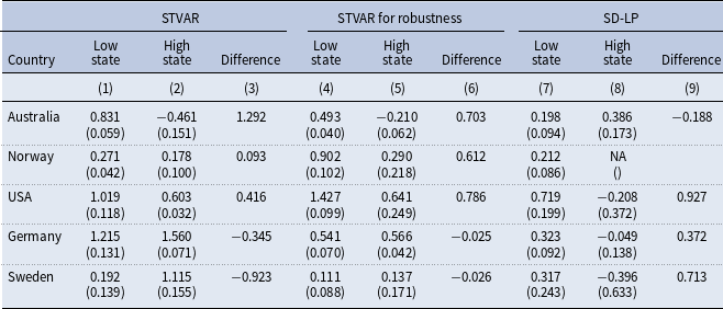
Notes: This table shows fiscal multiplers (on impact) estimated with smooth transition vector autoregression (STVAR) and state -depedent local projection (SD-LP) models. STVAR Robustness refers to the model that identifies a low regime with $F(z_{t}) \lt = 0.4$
and a high regime with
$F(z_{t}) \lt = 0.4$
and a high regime with $F(z_{t}) \gt = 0.6$
. NA stands for not available. NA indicates the model was not able to estimate the fiscal multiplier in the corresponding state.
$F(z_{t}) \gt = 0.6$
. NA stands for not available. NA indicates the model was not able to estimate the fiscal multiplier in the corresponding state.
STVAR vs state-dependent local projection: Government spending multipliers. Note: This figure shows a comparison between STVAR generalized impulse response functions and SD-LP impulse response functions for government spending for low and high states. In the case of Norway, the SD-LP model was not able to estimate the fiscal multiplier in the high state. We calculate these figures following the definition of fiscal multiplier presented in equation (6). Estimation sample for each country can be found in Table 2 in the appendix.

When comparing the spending multipliers estimated with STVAR generalized impulsed responses functions, Table 5 shows that for Australia, Norway, and the United States the fiscal multiplier (on impact) is larger when fiscal interventions take place during periods of low household debt. Furthermore, our robustness results also confirm our findings.
When comparing our initial and robustness results, it is informative to focus on the standard deviation of our estimations. While the precision of our results improves for Australia, the United States, Germany, and Sweden after changing the identification strategy for the low regime, this is not a general conclusion when we focus on high regime estimations. It can be observed that standard deviations decrease for some countries and increase for others.
On the other hand, fiscal multipliers (on impact) estimated with SD-LP impulse response functions indicate that the evidence is not conclusive about whether the impact of government spending is conditioned by the amount of household debt in the economy. For Australia, the spending multiplier is larger when government spending increases during periods of high household debt, whereas the result is the opposite for the United States, Germany, and Sweden. In agreement with Tanaka (Reference Tanaka2020), it can be observed the large dispersion of the SD-LP results.
Our results show that on average the fiscal multiplier (on impact) is 0.93, 0.37, and 0.71 (percent of GDP) larger in low-debt states for the United States, Germany, and Sweden when we use an SD-LP model. On the other hand, we find that on average the fiscal multiplier (on impact) is 0.19 (percent of GDP) larger in high-debt states for Australia. With respect to Norway, the SD-LP model does not identify the high state.
In terms of the magnitude of differences between low and high regimes in the STVAR and SD-LP models, our results do not indicate any particular model effect. This would be the case if the absolute value of the difference between low and high regimes in one of the models dominates the same absolute value in the other model. For example, the difference in the fiscal multiplier between low and high regimes is higher under the SD-LP model in the United States, but the same comparison for Australia shows that the difference is higher under the STVAR model. To sum up, we are able to state that the magnitude of the fiscal multiplier difference between low and high regimes is not dominated by any of the models chosen for the analysis.
Using an SD-LP model leads us to a similar conclusion as when we use a STVAR. Evidence about whether the impact of government spending is conditioned by the amount of household debt in the economy is not conclusive. The results from the SD-LP model suggest that for Australia, the spending multiplier is larger when government spending increases during periods of high household debt, whereas the result is the opposite for the United States, Germany, and Sweden.
6. Discussion
To date, few papers have explored whether rising household debt affects fiscal policy. In this paper, we analyzed whether the impact of government spending on economic output is conditioned by the level of household debt.
To test this hypothesis empirically, we used a smooth transition vector autoregression model to examine the government spending multiplier in periods of low and high household debt (low and high regimes) in Australia, Sweden, Norway, and the world’s seven largest economies. While financial cycles appear to be more commonly observed in developed economies, we acknowledge the potential to expand this research to include a broader range of economies, including developing countries.
Our model identifies an economy to be in a low or high-debt state if the value of the transition variable is below or above the point of inflection estimated by the model. We considered household debt-to-GDP ratio and residential housing prices as potential transition functions to capture changes between regimes. Our decision to include housing prices as a proxy of household debt was attributed to the findings of Terrones et al. (Reference Terrones, Claessens and Kose2011), who highlight a strong synchronization between housing prices and household debt during financial cycles.
Using Bayes factor criteria and based on the analysis of the transition function probability, we chose to examine the model results using household debt to GDP in the transition function for Australia, Sweden, the United States, Canada, the United Kingdom, and Germany, and residential housing prices in the transition function for Norway, Italy, France, and Japan.
Unfortunately, our model specification was unable to identify low- and high-debt regimes for Canada, the United Kingdom, Italy, France, and Japan. Most of the identification challenges are attributed to the difficulty of the transition function to remain either at the low or the high regime. Another reason is that the required magnitude of the change in the transition variable to trigger a regime shift is less likely to be observed in the sample. For these reasons, we only assessed the model results for Australia, Sweden, Norway, the United States, and Germany.
We found that the short-term effect (on impact) of government spending tends to be higher if fiscal expansion takes place during periods of low household debt. On average, the fiscal multiplier (on impact) is 0.70, 0.61, and 0.79 (percent of GDP) higher when the increase in government spending takes place during periods of low debt for Australia, Norway, and the United States. We also found that the medium and long-term effects of government spending remain uncertain no matter whether the fiscal expansion takes place during periods of low or high household debt. In agreement with Gonçalves et al. (Reference Gonçalves, Herrera, Kilian and Pesavento2022), this can be attributed to the difficulty of identifying different regimes for horizons greater than zero.
We studied the sensitivity of our results to changes in the point of inflection ( $c$
) parameter, which governs the transition between low and high regimes. We also explore the sensitivity of our findings to variations in the
$c$
) parameter, which governs the transition between low and high regimes. We also explore the sensitivity of our findings to variations in the $\gamma$
parameter, which determines the speed of transition between low and high-debt states. We found that our results are more sensitive to changes in the
$\gamma$
parameter, which determines the speed of transition between low and high-debt states. We found that our results are more sensitive to changes in the $c$
parameter rather than in the
$c$
parameter rather than in the $\gamma$
parameter.
$\gamma$
parameter.
We also examined our results after defining a new identification strategy that requires a higher likelihood to identify low- and high-debt regimes. We found that the more likely the economy to be in a high-debt state, the lower output responses are. It is worth noting that the standard deviations of our estimates were sensitive to the specifications of the model.
To evaluate the model’s effects in our results, we also estimated the fiscal multipliers with a SD-LP model. We found that measuring the impact of government spending with an SD-LP model affects the magnitude of the fiscal multiplier (on impact). In general, we found that the effect of government spending on GDP (on impact) tends to be higher if fiscal expansion takes place during periods of low household debt.
Last, but not least, it is important to mention that our posterior probabilities and the analysis of the transition function probability led us to use housing prices as a transition variable for Norway. As a robustness check, we also estimated state-dependent local projection impulse response functions when we considered household debt to GDP as a switching variable for this country. Our results, displayed in Table 7 in the appendix, confirm that the effect of government spending on output (on impact) tends to be higher if fiscal expansion takes place during periods of low household debt.
Our findings also contribute to the literature on fiscal multipliers in periods of low and high household debt. Contrary to Bernardini and Peersman (Reference Bernardini and Peersman2018), who found that fiscal multipliers are considerably larger during periods of high household debt in the United States, our research did not reveal higher spending multipliers during those periods. Our results for the United States suggest a larger fiscal multiplier during periods of low household debt. These findings led us to similar conclusions when examining the cases of Australia and Norway.
A potential explanation for the difference between Bernardini and Peersman (Reference Bernardini and Peersman2018) and our results could be that the fiscal expansion they analyze targets primarily households with high levels of debt, who have reduced their consumption to increase their housing assets. The consumption response of these households to a transfer may be stronger.
Another rationale for the disparity between Bernardini and Peersman (Reference Bernardini and Peersman2018) and our results is the identification of periods of low and high household debt, as well as the lag length selection in the model. In their study, they define low- and high-debt states as negative and positive deviations of the debt-to-GDP ratio from its long-term trend. This identification is subject to the definition of the trend, which may be influenced by the characteristics of the data, the objectives of the analysis, and the methodological preferences of the analyst (Pollock (Reference Pollock2016)). In contrast, our identification relies on a logarithm function that depends on two parameters: point of inflection ( $c$
) and smooth transition (
$c$
) and smooth transition ( $\gamma$
). Additionally, there is a disparity in lag length selection. While they choose lag
$\gamma$
). Additionally, there is a disparity in lag length selection. While they choose lag $p=4$
, we select lag
$p=4$
, we select lag $p=6$
. In fairness to Bernardini and Peersman (Reference Bernardini and Peersman2018), it is important to recognize that the choice of the lag in the STVAR model influences the magnitude of the fiscal multiplier.
$p=6$
. In fairness to Bernardini and Peersman (Reference Bernardini and Peersman2018), it is important to recognize that the choice of the lag in the STVAR model influences the magnitude of the fiscal multiplier.
Our results also extend the insights presented in Auerbach and Gorodnichenko (Reference Auerbach and Gorodnichenko2012)’ study, which shows that fiscal multipliers tend to be larger during economic recessions compared to economic expansions. Our findings underscore the importance of considering financial cycles, in addition to business cycles, when assessing the effectiveness of fiscal policy.
Our findings also contribute to the Keynesian versus Ricardian debate regarding the impact of fiscal expansions on aggregate demand.Footnote 3 The variation in fiscal multipliers between periods of low and high household debt tells us that high levels of household indebtedness condition households’ behavior following the receipt of a fiscal transfer, weakening the effect of fiscal expansions in the short term. This reveals a weakness in the Keynesian idea that fiscal expansions can take advantage of households’ positive marginal propensity to consume and stimulate the economy through an expansion of aggregate demand. On the other hand, our results do not inform about the long-term effects of fiscal policy, restricting us from reaching conclusions about whether the Ricardian Equivalence holds or not.
Our approach may also be susceptible to certain limitations. We estimated an STVAR model with steady-state priors. As highlighted by Chan and Koop (Reference Chan and Koop2014), it is plausible that some or all steady states may change over time due to modifications in the political and economic context. This is a possible limitation in our analysis and creates opportunities for future research. Additionally, our approach does not distinguish between expected and unexpected shocks to government spending, providing a potential avenue for further research.
In further research, the impact of household debt on fiscal stimulus should be considered in the context of both short and long-term debt, and debt borrowed to fund durable and non-durable consumption. Similarly, the model could be extended with the inclusion of government debt as an endogenous variable or as a transition variable. This would help to clarify whether the fiscal multiplier is a negative function of government debt as asserted by Perotti (Reference Perotti1999). It would also contribute to exploring the potential presence of crowding-out effects between government and household debt. Contributions based on microdata, as in Demyanyk et al. (Reference Demyanyk, Loutskina and Murphy2019), could add substantial value to exploring the mechanism through which debt overhang conditioned the impact of fiscal expansions.
7. Conclusion
In this paper, we study whether household debt affects the size of the fiscal multiplier and whether the impact of government expenditure is conditioned by the amount of household debt in the economy.
Our findings suggest that the magnitude of the fiscal multiplier during periods of low and high household debt varies across countries, and the methodology employed to identify low- and high-debt regimes plays a crucial role. Based on our empirical evidence, we concluded that the short-term effects of government spending tend to be higher if fiscal expansion takes place during periods of low household debt. However, it is still unclear whether different levels of household debt have a significant influence on government spending multipliers in the medium and long term.
On average, the fiscal multiplier (on impact) is 0.70, 0.61, and 0.79 (percent of GDP) larger when the increase in government spending takes place during periods of low household debt for Australia, Norway, and the United States.
Our results are also robust to changes in the identification strategy. Changing the approach used to identify low and high-debt regimes does not alter our conclusions about the size of the fiscal multiplier (on impact) for the countries mentioned above. Contrary to Bernardini and Peersman (Reference Bernardini and Peersman2018), who found that fiscal multipliers are considerably larger during periods of high household debt in the United States, we did not find higher spending multipliers during those periods.
Our results have significant policy implications. They highlight the importance of taking into account financial cycles, as well as business cycles, to evaluate the effectiveness of fiscal policy. Where there is a high level of household debt in the economy, the necessary fiscal expansion to reach the same output response will be higher. As household debt increases and borrowing constraints relax, the importance of targeting fiscal policy increases (Kaplan and Violante (Reference Kaplan and Violante2014)).
Future studies could seek to replicate our empirical results using government capital expenditure instead of government consumption expenditure or examine how household debt may affect the taxation fiscal multiplier. Future research would also consider including government debt in the model specification. It would also be positive to find microeconomic evidence that helps to understand empirically the effect of household debt on the marginal propensity to consume after receiving a fiscal transfer. This may help to draw better conclusions about the importance of the consumption channel in determining the magnitude of the output response triggered by fiscal stimulus. We hope our results attract researchers interested in continuing to explain the role that household debt plays in policy interventions more generally.
Acknowledgments
This paper has greatly benefited from discussions with Mengheng Li, Corrado Di Guilmi, Jorge Miranda-Pinto, Gordon Menzies, Peter Docherty, Mariano Kulish, and Chung Tran, as well as participants at the Continuing Education in Macroeconometric Workshop 2023. I would like to thank the anonymous referees of Macroeconomic Dynamics for valuable comments that improved the quality of the paper. Any remaining errors are the author’s responsibility.
Supplementary material
To view supplementary material for this article, please visit https://doi.org/10.1017/S1365100524000075


 Open access