1. Introduction
In linear mixed models, it is often assumed that the residual variance is homogeneous. However, differences in the residual variance among individuals are quite common and it is important to include the effect for heteroscedastic residuals in models for traditional breeding value evaluation (Hill, Reference Hill1984). Such models, having explanatory variables accounting for heteroscedastic residuals, are routinely used by breeding organizations today. The explanatory variables are typically non-genetic (Meuwissen et al., Reference Meuwissen, de Jong and Engel1996; Yang et al., Reference Yang, Schön and Sorensen2012), but genetic heterogeneity can be present and it is included as a random effect for the residual variance part of the model.
Product uniformity is often a desirable breeding goal. Therefore, we need methods to estimate both variance components and breeding values in the residual variance part of the model to be able to select animals that can satisfy this goal. Moreover, if genetic heterogeneity is present then traditional methods for predicting selection response can be misleading (Hill & Zhang, Reference Hill and Zhang2004; Mulder et al., Reference Mulder, Bijma and Hill2007).
Methods have previously been developed to estimate the degree of genetic heterogeneity. SanCristobal-Gaudy et al. (Reference SanCristobal-Gaudy, Elsen, Bodin and Chevalet1998) have developed a likelihood-based expectation-maximization (EM) algorithm. Sorensen & Waagepetersen (Reference Sorensen and Waagepetersen2003) have applied a Bayesian Markov chain Monte Carlo (MCMC) algorithm to estimate the parameters in a similar model, which has the advantage of producing model-checking tools based on posterior predictive distributions and model-selection criteria based on the Bayes factor and deviances. At the same time, Bayesian methods to fit models with residual heteroscedasticity for multiple breed evaluations (Cardoso et al., Reference Cardoso, Rosa and Tempelman2005) and generalized linear mixed models allowing for a heterogenetic variance term (Kizilkaya & Tempelman, Reference Kizilkaya and Tempelman2005) have been developed. Wolc et al. (Reference Wolc, White, Avendano and Hill2009) have studied a sire model, with random genetic effects included in the residual variance, by fitting squared residuals with a gamma generalized linear mixed model. Mulder et al. (Reference Mulder, Hill, Vereijken and Veerkamp2009) fitted a bivariate linear model for the trait and the log-squared residuals, and they estimated the correlation between effects for mean and variance. Hill & Mulder (Reference Hill and Mulder2010) reviewed the topic of genetic control of environmental variation. Yang et al. (Reference Yang, Christensen and Sorensen2011) showed that inferences under the genetically structured heterogeneous variance model can be misleading when the data are skewed.
Lee & Nelder (Reference Lee and Nelder2006) developed their framework of double hierarchical generalized linear models (DHGLM), which has been applied to stochastic volatility modelling in finance (del Castillo & Lee, Reference del Castillo and Lee2008) and also to robust inference against outliers by allowing heavy tailed distributions (Lee & Nelder, Reference Lee and Nelder2006). Inference in DHGLM is based on hierarchical likelihood (h-likelihood) theory (Lee & Nelder, Reference Lee and Nelder1996) and DHGLM is a direct extension of hierarchical GLM (HGLM) including random effects for the dispersion. Two main computational strategies are available. In the first, the parameters are estimated by iterating a hierarchy of generalized linear models (GLM), where each GLM is estimated by iterative reweighted least squares (IRWLS; see e.g. Rönnegård et al., Reference Rönnegård, Shen and Alam2010). The second strategy works by numerically maximizing the h-likelihood (see e.g. Molas & Lesaffre, Reference Molas and Lesaffre2011). The first is computational fast, while the other may produce higher-order estimators (Noh & Lee, Reference Noh and Lee2007). DHGLM give model checking tools based on GLM theory and model-selection criteria are calculated from the h-likelihood (Lee & Nelder, Reference Lee and Nelder1996). Both the theory and the fitting algorithm are explained in detail in Lee et al. (Reference Lee, Nelder and Pawitan2006).
Rönnegård et al. (Reference Rönnegård, Shen and Alam2010) used DHGLM to estimate breeding values for mean and dispersion in an animal model, and also their variances, but the correlation between them was not included. The computational demands were decreased compared with Markov chain Monte Carlo estimation. The method by Rönnegård et al. (Reference Rönnegård, Felleki, Fikse, Mulder and Strandberg2010) can be used to estimate genetic heterogeneity of the residual variance in animal models with many observations.
Previously correlation between random effects for the same level in DHGLM have been estimated (Lee et al., Reference Lee, Nelder and Pawitan2006), i.e. correlation between random effects for the mean, or correlation between random effects for the dispersion. Correlation between random effects for different levels, that is between an effect for the mean model and an effect for the residual variance model, has not previously been reported within the DHGLM framework.
The aim of this paper is to extend DHGLM, and thereby the method from Rönnegård et al. (Reference Rönnegård, Felleki, Fikse, Mulder and Strandberg2010), to include correlation between random effects for mean and variance, and moreover to evaluate the performance with regard to bias and precision.
2. Material and methods
In this section, we start by defining the exponential model (Hill & Mulder, Reference Hill and Mulder2010) introduced by SanCristobal-Gaudy et al. (Reference SanCristobal-Gaudy, Elsen, Bodin and Chevalet1998). Thereafter, a bivariate linear mixed model is used as a tool in an IRWLS algorithm for fitting the exponential model. The algorithm is a natural extension of the algorithm by Rönnegård et al. (Reference Rönnegård, Shen and Alam2010) by including a correlation between random effects for mean and variance. It is also quite similar to the one presented by Mulder et al. (Reference Mulder, Hill, Vereijken and Veerkamp2009), except that the algorithm below corrects for the fact that estimated, and not true, residuals are used, and that the squared residuals are gamma distributed. In the Appendix, we derive that the IRWLS algorithm can be motivated using the h-likelihood method.
(i) Model
The model fitted is the exponential model,
 $${\rm E}\lpar y\vert a\comma a_{d} \rpar \equals \mu $$
with a linear predictor
 $$\mu \equals X\beta \plus Za.$$
The dispersion part of the model is specified as
 $${\rm var}\lpar y\vert a\comma a_{d} \rpar \equals \rmPhi $$
with linear predictor
 $$\rmPhi \equals {\rm diag}\ \phi \comma \quad {\rm log}\ \phi \equals X_{d} \beta _{d} \plus Za_{d} .$$
By y is denoted a vector of n responses depending on fixed effects β and random effect a (length k), and φ is a vector of residual variances depending on fixed effects βd and random effect ad. The response vector y given a and ad is normal distributed. Matrices for design X and Xd, and the incidence matrix Z are known.
The random effects a and ad are normal distributed additive genetic effects with mean 0 and variance
 $${\rm var}\left( {\matrix{ a \cr {a_{d} } \cr} } \right) \equals G \otimes A\comma $$
 $$G \equals \left( {\matrix{ {\sigma _{a}^{\setnum{2}} } \tab {\sigma _{a} \sigma _{a_{d} } \rho } \cr {\sigma _{a} \sigma _{a_{d} } \rho } \tab {\sigma _{a_{d} }^{\setnum{2}} } \cr} } \right)\comma $$
where A is the additive genetic relationship matrix of dimension k for the additive genetic effects, thus σa 2A is the covariance of a and  $\sigma _{a_{d} }^{\setnum{2}}$A is the covariance of ad. The parameter ρ is the correlation between a and ad as included in the estimation by Sorensen & Waagepetersen (Reference Sorensen and Waagepetersen2003).
The model on responses y is referred to as the mean part, and the model on the residual variances φ is referred to as the residual variance part. Other uncorrelated random effects (permanent environmental effects) can be added to both the mean and the residual variance parts.
The additive genetic effect ad for the residual variance log φ is the genetic control of environmental variation, which is a measure on the uniformity of trait expression. The correlation parameter ρ indicates how the uniformity varies with the breeding value of the animal. A numerically high value of ρ would mean that selection of high breeding values for the mean would change the environmental variance.
(ii) A bivariate linear mixed model and a fitting algorithm
Consider the bivariate linear mixed model
 $$\eqalign{\left( {\matrix{ y \cr {z_{d} } \cr} } \right) \equals \tab \left( {\matrix{ X \tab 0 \cr 0 \tab {X_{d} } \cr} } \right)\left( {\matrix{ \beta \cr {\beta _{d} } \cr} } \right) \cr \tab \plus \left( {\matrix{ Z \tab 0 \cr 0 \tab Z \cr} } \right) \left( {\matrix{ a \cr {a_{d} } \cr} } \right) \plus \left( {\matrix{ e \cr {e_{d} } \cr} } \right)\comma} $$
with working weight matrix and residual variance
 $$\rmSigma ^{ \minus \setnum{1}} \equals \left( {\matrix{ {\rmPhi ^{ \minus \setnum{1}} } \tab 0 \cr 0 \tab {{\rm diag}\lpar {{1 \minus q} \over 2}\rpar } \cr} } \right)\comma \quad {\rm var}\left( {\matrix{ e \cr {e_{d} } \cr} } \right) \equals \rmSigma \left( {\matrix{ {\sigma ^{\setnum{2}} I_{n} } \tab 0 \cr 0 \tab {\sigma _{d}^{\setnum{2}} I_{n} } \cr} } \right).$$
Here the residual variances σ2 and σd 2 are both 1 (but defined for later use in the fitting algorithm below), zd is the vector of linearized working variables (McCullagh & Nelder Reference McCullagh and Nelder1989)
 $$z_{d\comma i} \equals {\rm log}\ \phi _{i} \plus \phi _{i}^{ \minus \setnum{1}} \left( {{{\hat{e}_{i}^{\setnum{2}} } \over {1 \minus q_{i} }} \minus \phi _{i} } \right)\comma $$
and q is the vector of hat values defined in Appendix (i)(b).
This gives estimates similar to h-likelihood estimates, as shown in the Appendix. We call the bivariate REML method used to fit the linear mixed model above an IRWLS approximation of the h-likelihood.
Fitting algorithm for the IRWLS approximation
The above linear mixed model (3) is fitted by the following IRWLS algorithm.
(1) Initialize weights $\rmSigma ^{ \minus \setnum{1}} \equals \left( {\matrix{ {\rmPhi ^{ \minus \setnum{1}} } \hfill \tab 0 \hfill \cr 0 \hfill \tab {{\rm diag}\left( {{\textstyle{{1 \minus q} \over 2}}} \right)} \hfill \cr} } \right)$ and working variables zd.
(2) Fit (3) with correlation structure G⊗A between a and ad, but y and zd conditional uncorrelated, that is, var(y|a, ad) = σ2Φ and var(zd|a, ad) = σd 2diag(2/(1−q)).
(3) Update
$\mathop {\hat{\sigma }}\nolimits^{\setnum{2}} $, ê and q, and thereby $z_{d} \equals {\rm log}\lpar \mathop {\hat{\sigma }}\nolimits^{\setnum{2}} \phi \rpar \plus {\textstyle{1 \over {\mathop {\hat{\sigma }}\nolimits^{\setnum{2}} }}}\rmPhi ^{ \minus \setnum{1}} \lpar \mathop {\hat{e}}\nolimits^{\setnum{2}} \sol \lpar 1 \minus q\rpar \minus \mathop {\hat{\sigma }}\nolimits^{\setnum{2}} \phi \rpar $ and diag((1−q)/2) in Σ−1.(4) Repeat step 2.
(5) Update
$\rmPhi ^{ \minus \setnum{1}} \equals {\rm diag}\lpar {\rm exp}\lpar \mathop {\hat{z}}\nolimits_{d} \rpar \rpar ^{ \minus \setnum{1}} $ and update Σ−1.(6) Iterate steps 2–5 until convergence (
$\mathop {\hat{\sigma }}\nolimits^{\setnum{2}} \equals 1$).


(iii) Simulations for validating the h-likelihood method
Estimation of correlation between random effects for mean and dispersion is new within the h-likelihood framework and there are potential applications in other research areas than genetics. A relatively simple simulation structure was therefore considered. Using these simulations the h-likelihood method and the IRWLS approximation were compared. The h-likelihood was implemented in the R software using a Newton–Raphson algorithm on the score functions. The score functions are given in the Appendix for the effects for mean and variance, together with the adjusted profile likelihood for the variance components. The variance components were estimated using transformation  $\xi \equals \lpar {\rm log}\ \sigma _{a}^{\setnum{2}} \comma {\rm log}\ \sigma _{a_{d} }^{\setnum{2}} \comma {\rm log}\ {\textstyle{{1 \plus \rho } \over {1 \minus \rho }}}\rpar $ to avoid boundary problems.
We simulated 10 000 observations and a random group effect. The number of groups was either 10 or 100. An observation for individual j with covariate x belonging to group k was simulated as yjk = 1·0x+ak+e jk, where the random group effects were iid with ak∼N(0,σa 2), and the residual effect ejk was sampled from N(0, var(ejk)) with var(ejk) = exp(0·2x+ad ,k). The covariate x was simulated binary to resemble sex effect. Furthermore,  $a_{d\comma k} \sim N\lpar 0\comma \sigma _{a_{d} }^{\setnum{2}} \rpar $ with ${\rm cov}\lpar a_{k} \comma a_{d\comma k} \rpar \equals \rho \sigma _{a} \sigma _{a_{d} } $. The simulated variance components were σa 2 = 1 and $\sigma _{a_{d} }^{\setnum{2}}$=0·1 or 0·5, whereas the correlation ρ was either −0·5 or 0·95. The value of $\sigma _{a_{d} }^{\setnum{2}}$=0·1 gives a substantial variation in the simulated elements of ad, where one standard deviation difference between two values ad ,l and ad ,m increases the residual variance 1·37 times. We replicated the simulation 100 times and obtained estimates of variance components using the h-likelihood method and the IRWLS algorithm.
The computational demands of the h-likelihood method, implemented in R, limited analyses of more sophisticated unbalanced data scenarios and were therefore not used in the following analyses.
(iv) Pig litter size data and model
Pig litter size was previously analysed by Sorensen & Waagepetersen (Reference Sorensen and Waagepetersen2003) using the Bayesian method, and the data are described therein. The data includes 10 060 records from 4149 sows and a total number of 6437 pigs in the pedigree. Hence, repeated measurements on sows were present and a permanent environmental effect of each sow was included in the model. The maximum number of parities is nine. The data include the following class variables: herd (82 classes), season (four classes), type of insemination (two classes) and parity (nine classes). The data are highly unbalanced; 13 herds contribute five observations or less, and the ninth parity includes nine observations.
Several models were analysed by Sorensen & Waagepetersen (Reference Sorensen and Waagepetersen2003) with an increasing level of complexity in the model for the residual variance, and with the model for the mean y=Xβ+Wp+Za+e. Here y is the litter size (vector of length 10 060), β is a vector including the fixed effects of herd, season, type of insemination and parity, and X is the corresponding design matrix (10 060 × 94), p is the random permanent environmental effect (vector of length 4149), W is the corresponding incidence matrix (10 060×4149) and var(p) = σp 2I, a is the random additive genetic effect, Z is the corresponding incidence matrix (10 060×6437) and var(a) = σa 2A, where A is the additive relationship matrix. Hence, the LHS of the mixed model equations is of size 10 680 × 10 680.
The residual variance var(e) was modelled as follows, where Model III and Model IV are model names from Sorensen & Waagepetersen (Reference Sorensen and Waagepetersen2003) :
Model III: Random additive genetic effect and fixed effects for the linear predictor for the residual variance
 $${\rm var}\lpar e_{i} \rpar \equals {\rm exp}\lpar X_{d\comma i} \beta _{d} \plus Z_{i} a_{d} \rpar \comma $$
where βd is a parameter vector including an intercept β0 and effects of parity and type of insemination, Xd ,i is the ith row in the design matrix Xd, Zi is the ith row of Z, and ad is the random additive genetic effect.
Model IV: Permanent environmental effect, additive genetic effect, and fixed effects for the linear predictor for the residual variance
 $${\rm var}\lpar e_{i} \rpar \equals {\rm exp}\lpar X_{d\comma i} \beta _{d} \plus W_{i} p_{d} \plus Z_{i} a_{d} \rpar \comma $$
where Wi is the ith row of W and pd is a random permanent environmental effect with  $p_{d} \sim N\lpar 0\comma \sigma _{p_{d} }^{\setnum{2}} I\rpar $.
(v) Simulations for validating the IRWLS approximation
To test whether the IRWLS algorithm gives unbiased variance components on realistic examples for animal breeding, we simulated observations using the pedigree from the pigs litter size data. The number of sows with records was fixed as in the original dataset. The total number of observations was either kept (n = 10 060), or increased by changing the number of repeated records per sow (parities) to 4 (n = 4 × 4149 = 16 596) or 9 (n = 9 × 4149 = 37 341).
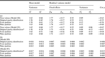
On the mean level the observation for animal j, parity k and insemination type x was yjk = 11·16 + βparity,k + 0·45x+pj+aj+ejk. The residual effect was sampled from N(0,var(ejk)) with var(ejk) = exp(1·77 + βd,parity,k − 0·17x+pd ,j+ad ,j). Additive genetic effects were sampled from (2) with σa 2 = 1·62, $\sigma _{a_{d} }^{\setnum{2}}$=0·09 and ρ = −0·62. Permanent environmental effects were sampled from pj∼N(0, 0·60) and pd ,j∼N(0, 0·06) (Model IV) or pd ,j = 0 (Model III). These values came from Sorensen & Waagepetersen (Reference Sorensen and Waagepetersen2003). The simulations were replicated 100 times and analysed using the IRWLS algorithm.
3. Results
(i) Simulations for validating the h-likelihood method
For the simulations with balanced data, the two methods h-likelihood and IRWLS gave identical results (Table 1) up to the fourth decimal. When the number of groups was small (10 groups), there was a large variation in the estimates, because only ten values of a and ad were sampled in each replicate. In that case there was a tendency for ρ to be overestimated (estimate −0·42, 16% overestimated) because of the parameter boundary ρ ⩾ −1. An alternative way to estimate ρ is to take mean of log((1 + ρ)/(1 − ρ)). By doing that we avoid boundary problems and obtained the value −0·48 (4% overestimated).
Mean (standard errors) for 100 replicates of 10 000 balanced observations in k groups using the h-likelihood estimator. (The IRWLS algorithm gave identical results)

* Results in the fourth row are calculated from 58 replicates that converged for both methods (97 replicates converged for the h-likelihood method and 60 replicates converged for the IRWLS algorithm).
The algorithms performed well for estimating variance components for models with correlation between random effects for mean and residual variance.
(ii) Data on pigs litter sizes
For the pigs litter size data, the results for the IRWLS algorithm (Table 2) were similar to the MCMC estimates of Sorensen & Waagepetersen (Reference Sorensen and Waagepetersen2003) for most parameters. The MCMC estimates of ρ were slightly more negative (−0·57 for Model III and −0·62 for Model IV) than the IRWLS estimates (−0·49 for Model III and −0·52 for Model IV). Similarity of estimates for the two methods was found for the variance components σa 2 and  $\sigma _{p_{d} }^{\setnum{2}} $, and for all of the fixed effects for the residual variance, βd. The permanent environmental effect variance σp 2 in the mean model was about half the MCMC estimate, and the additive genetic variance $\sigma _{a_{d} }^{\setnum{2}} $ in the residual variance was considerably larger, compared with Sorensen & Waagepetersen (Reference Sorensen and Waagepetersen2003).
Estimates and 95% confidence intervals of chosen parameters for pigs litter size data in Model III (first section) and Model IV (second section) used by Sorensen & Waagepetersen (Reference Sorensen and Waagepetersen2003). Results obtained by Sorensen & Waagepetersen (Reference Sorensen and Waagepetersen2003) (first row in each section), by Rönnegård et al. (Reference Rönnegård, Shen and Alam2010) (second row) and using IRWLS (third row)

* βd 0 is the intercept term in the model for the residual variance,  $\beta _{{d} _{\rm ins}} $ is the fixed effect for insemination and $\beta _{{d} _{\rm par}} $ is the fixed effect for the difference in first and second parity.
(iii) Simulations for validating the IRWLS approximation
The general trend showed that bias and standard error (SE) decreased when the number of parities was increased for each sow (Table 3). There were exceptions to this trend, including the intercept term βd 0 of Model IV, which could be due to the fact that the number of parities for some sows was actually smaller in the setting with four parities for all sows compared with the original data structure. For the scenario with nine parities per sow, both bias and SE were very small or negligible for all parameters.
Mean (a) and standard errors (b) of estimates of parameters for simulated data over Model III (first section) and Model IV (second section). The left hand column contains the simulated data structure

* Twenty-seven out of 100 replicates did not converge. Estimates are for all replicates (with minor differences in results if these 27 replicates were included or not).
The estimates of $\sigma _{a_{d} }^{\setnum{2}} $ and ρ were biased for Model III, and Model IV seems to be more appropriate to use for situations with repeated observations. For Model IV, the magnitude in percentage bias was less than 10% for all parameters except the permanent environmental effects for the mean and residual variance models (i.e. σp 2 and $\sigma _{p_{d} }^{\setnum{2}} $) (Table 3 (b)). The genetic parameters σa 2, $\sigma _{a_{d} }^{\setnum{2}} $ and ρ were estimated with small or no bias, for all scenarios and both models, indicating that the method will give good estimates for these parameters in a very general setting.
4. Discussion
We have extended the DHGLM framework to include correlation between random effects for the mean and the residual variance, for a normal response and normal distributed random effects. We have approximated the h-likelihood by an IRWLS algorithm that in summary works by iteratively updating and fitting a bivariate linear mixed model simultaneously on mean and residual variance. The IRWLS approximation of DHGLM is a fast and easily implemented algorithm for genetic heterogeneity estimation building on REML tools. The additional functions required are implemented in the developmental version of ASReml (Gilmour, Reference Gilmour2010) to be released as ASReml 4 and an example code is available on request from the authors.
Significant bias was found for data structures having few repeated observations per individual, where the bias decreased quickly as the number of repeated observations increased. For data structures having few repeated observations, the largest bias was detected for σp 2. This is perhaps not surprising, because for an individual having a single observation the permanent environmental effect pi and the residual ei are indistinguishable, and part of the σp 2 will therefore be picked up by the residual variance.
It is possible that more accurate estimates could be obtained by implementing a computationally efficient algorithm (using sparse matrix techniques) for the h-likelihood estimation method presented in our paper, instead of using the IRWLS algorithm. This would, however, require further research. Furthermore, the second-order h-likelihood estimation method is known to eliminate bias for binary outcomes in HGLM (Lee et al., Reference Lee, Nelder and Pawitan2006), but can be more demanding to compute.
Similar bias patterns were found when comparing the simulation study with the difference between the estimates obtained by Sorensen & Waagepetersen (Reference Sorensen and Waagepetersen2003) and the IRWLS estimates (Tables 2 and 3). The variance components for the mean model, the fixed effects for the residual variance and the correlation showed a similar pattern in differences. This might give an indication of a problem with the IRWLS estimates being biased in certain directions, when the data structure does not contain enough repeated observations to give good estimates. However, variance components for the residual variance did not follow the same pattern. A simulation study using Bayesian MCMC methods would be desirable but is not within the scope of the current paper.
The IRWLS algorithm is distinct from the algorithm used by Mulder et al. (Reference Mulder, Hill, Vereijken and Veerkamp2009) because it uses h-likelihood theory and the algorithm fits corrected squared residuals as a gamma distributed response, whereas the log-squared residuals were fitted as a normal response in Mulder et al. (Reference Mulder, Hill, Vereijken and Veerkamp2009). Compared with Bayesian methods we expect the IRWLS algorithm to be faster. The IRWLS computation on pigs litter size data took less than 5 min on a Linux server.
In a previous paper, Rönnegård et al. (Reference Rönnegård, Shen and Alam2010), the variance part was fitted using a gamma generalized linear mixed model. In the presented IRWLS algorithm, we could have fitted a bivariate normal-gamma model, but chose to fit a corresponding bivariate normal–normal model that gives the same estimates at convergence. The bivariate normal–normal model resulted in a user-friendly code and is straightforward to compare with the method in Mulder et al. (Reference Mulder, Hill, Vereijken and Veerkamp2009). However, the bivariate normal–gamma model can be implemented by iteratively calling ASReml using some external code (in R or Fortran for instance). This approach may be required if convergence problems for the IRWLS algorithm occur, but perhaps more importantly the user should assess whether the available data are sufficient to be able to fit the model. When the number of repeated observations is too small (or with a single record per animal) there might not be enough information to fit a model with random additive genetic effects both for the mean and residual variance models.
Inferences under the genetically structured heterogeneous variance model can be misleading when the data are skewed (Yang et al., Reference Yang, Christensen and Sorensen2011). In analysis of data using DHGLM, scaling effects should be tested and a possibility would be to fit the IRWLS algorithm for different transformations of y combined with model selection tools to find an optimal transformation. This would, however, require further theoretical developments of the DHGLM approach.
The IRWLS algorithm provides a simple implementation of genetic heterogeneity models in existing REML estimation software useful in applied animal breeding and can deal with large datasets. We have focused on applications in animal breeding but the DHGLM framework is applicable in many other fields of research as well (including finance and industrial quality control (Lee et al., Reference Lee, Nelder and Pawitan2006; Lee & Nelder, Reference Lee and Nelder2006)), and we expect the interest in our theoretical development reaches beyond animal breeding.
5. Declaration of interests
The authors declare that they have no competing interests.
This project was partly financed by the RobustMilk project, which is financially supported by the European Commission under the Seventh Research Framework Programme, Grant Agreement KBBE-211708. The content of this paper is the sole responsibility of the authors, and it does not necessarily represent the views of the Commission or its services. LR recognizes financial support from the Swedish Research Council FORMAS. We thank Md. Moudud Alam, Freddy Fikse, Han Mulder and Erling Strandberg for useful comments on the manuscript.
Appendix IRWLS approximation of h-likelihood
We state the h-likelihood for the exponential model (1) and show that the IRWLS fitting algorithm for the bivariate linear mixed model (3) can be derived from it using an approximation. The h-likelihood will be maximized to estimate fixed and random effects for the mean part, an adjusted profile likelihood will be used to estimate fixed and random effects for the variance part, and from an additional profiling the estimates of variance components will be found. Adjusted profile likelihood corresponds to restricted maximum likelihood.
(i) The h-likelihood for the exponential genetic heterogeneity model
From Lee & Nelder (Reference Lee and Nelder1996), the h-likelihood (ignoring constant terms) is
 $$\eqalign{ h \equals \tab {\rm log} \ f\lpar y\vert a\comma a_{d} \rpar \plus {\rm log} \ f\lpar a\comma a_{d} \rpar \cr \equals \tab \minus {1 \over 2}{\rm log} \, {\rm det}\rmPhi \minus {1 \over 2}\lpar y \minus \mu \rpar ^{\rm T} \rmPhi ^{ \minus \setnum{1}} \lpar y \minus \mu \rpar \cr \tab \minus {1 \over 2}{\rm log}{\kern 1pt} {\rm det} G \otimes A \minus {1 \over 2}\mathop {\left( {\matrix{ a \cr {a_{d} } \cr} } \right)}\nolimits^{\rm T} G^{ \minus \setnum{1}} \otimes A^{ \minus \setnum{1}} \left( {\matrix{ a \cr {a_{d} } \cr} } \right). \cr} $$
This can be simplified as follows (ignoring a constant involving log det A):
 $$\eqalign{ h \equals \tab \minus {1 \over 2}\mathop\sum\limits_{i} \,{\rm log}\ \phi _{i} \minus {1 \over 2}\mathop \sum\limits_{i} \,\lpar y_{i} \minus \mu _{i} \rpar ^{\setnum{2}} \sol \phi _{i} \cr \tab \minus {k \over 2}\lcub {\rm log}\lpar \sigma _{a}^{\setnum{2}} \rpar \plus {\rm log}\lpar \sigma _{a_{d} }^{\setnum{2}} \rpar \plus {\rm log}\lpar 1 \minus \rho ^{\setnum{2}} \rpar \rcub \cr \tab \minus {1 \over {2\lpar 1 \minus \rho ^{\setnum{2}} \rpar }}\left( {{1 \over {\sigma _{a}^{\setnum{2}} }}a^{\rm T} A^{ \minus \setnum{1}} a \plus {1 \over {\sigma _{a_{d} }^{\setnum{2}} }}\mathop {a_{d} }\nolimits^{\rm T} A^{ \minus \setnum{1}} a_{d} } \right) \cr \tab \plus {\rho \over {\lpar 1 \minus \rho ^{\setnum{2}} \rpar \sqrt {\sigma _{a}^{\setnum{2}} \sigma _{a_{d} }^{\setnum{2}} } }}a^{\rm T} A^{ \minus \setnum{1}} a_{d} . \cr} $$
Lee & Nelder (Reference Lee and Nelder2001) considered the adjusted profile (log)- likelihood, which is defined by the generic function:
 $$p_{\alpha } \lpar l\rpar \equals \lsqb l \minus {\scale65%{1 \over 2}} {\rm \,log\ det} \lcub D\lpar l\comma \alpha \rpar \sol \lpar 2\pi \rpar \rcub \rsqb \vert _{\alpha \equals \tilde{\alpha }} \comma $$
where l is a likelihood (either a log marginal-likelihood or an h-likelihood) with nuisance effects α, D(l, α) = −∂2l/∂α2 and  $\tilde{\alpha }$ solves ∂l/∂α = 0. When profiling out random effects, it is an extension of the REML likelihood and used for estimating variance components. Furthermore, from a classical likelihood point of view, profiling out random effects is a Laplace approximation of an integrated (marginal) likelihood (Molas & Lesaffre, Reference Molas and Lesaffre2011).
A summarization of parameters and the functions from which they are estimated using h-likelihood is found in Table A.1. For the estimation one uses h for τM = (β, a),  $p_{\tau _{M} } \lpar h\rpar $ for τD = (βd, ad) and $p_{\tau } \lpar h\rpar \equals p_{\beta _{a}\comma \beta _{d} \comma a\comma a_{d} } \lpar h\rpar $ for $\xi \equals \lpar {\rm log}\sigma _{a}^{\setnum{2}} \comma {\rm log}\sigma _{a_{d} }^{\setnum{2}} \comma {\rm log}{\textstyle{{1 \plus \rho } \over {1 \minus \rho }}}\rpar $. The fixed and the random effects are found by solving the score equations:
 $$\left( {\matrix{ {{{\partial h} \over {\partial \tau _{M} }}} \cr {\vskip6pt{{\partial p_{\tau _{M} } \lpar h\rpar } \over {\partial \tau _{D} }}} \cr} } \right) \equals \left( {\matrix{ 0 \cr 0 \cr} } \right)$$
and the variance components by
 $${{\partial p_{\tau } \lpar h\rpar } \over {\partial \xi }} \equals 0.$$
Parameters and the functions from which they are estimated by using h-likelihood and the IRWLS algorithm

(a) Estimation of τM = (β, a)
The score function for τM = (β, a) is
 $$\eqalign{ \tab \hskip-2pt S\lpar \tau _{M} \rpar \equals {{\partial h} \over {\partial \tau _{M} }} \cr \tab \hskip-3.5pt \equals \left( {\matrix{ {X^{\rm T} \rmPhi ^{ \minus \setnum{1}} \lpar y \minus \mu \rpar } \hfill \cr {Z^{\rm T} \rmPhi ^{ \minus \setnum{1}} \lpar y \minus \mu \rpar \hskip-1pt \minus \hskip-1pt {1 \over {\lpar 1 \minus \rho ^{\setnum{2}} \rpar \sigma _{a}^{\setnum{2}} }}A^{ \minus \setnum{1}} a \hskip-1pt \plus \hskip-1pt {\rho \over {\lpar 1 \minus \rho ^{\setnum{2}} \rpar \sqrt {\sigma _{a}^{\setnum{2}} \sigma _{a_{d} }^{\setnum{2}} } }}A^{ \minus \setnum{1}} a_{d} } \hfill \cr} } \right)\comma} $$
and zero is given by the mixed model equation
 $$\eqalign{ \tab \left( {\matrix{ {X^{\rm T} \rmPhi ^{ \minus \setnum{1}} X} \tab \hskip-56pt {X^{\rm T} \rmPhi ^{ \minus \setnum{1}} Z} \cr {Z^{\rm T} \rmPhi ^{ \minus \setnum{1}} X} \tab {Z^{\rm T} \rmPhi ^{ \minus \setnum{1}} Z \plus {1 \over {\lpar 1 \minus \rho ^{\setnum{2}} \rpar \sigma _{a}^{\setnum{2}} }}A^{ \minus \setnum{1}} } \cr} } \right)\left( {\matrix{ \beta \cr a \cr} } \right) \cr \tab \equals \left( {\matrix{\hskip-82pt {X^{\rm T} \rmPhi ^{ \minus \setnum{1}} y} \cr {Z^{\rm T} \rmPhi ^{ \minus \setnum{1}} y \plus {\rho \over {\lpar 1 \minus \rho ^{\setnum{2}} \rpar \sqrt {\sigma _{a}^{\setnum{2}} \sigma _{a_{d} }^{\setnum{2}} } }}A^{ \minus \setnum{1}} a_{d} } \cr} } \right). \cr} $$
(b) Estimation of τD = (βd, ad)
For estimating τD = (βd, ad), we use the adjusted profile likelihood
 $$p_{\tau _{M} } \lpar h\rpar \equals \lsqb h \minus {\scale65%{1\over 2}} \ {\rm log \ det}\lcub D\lpar h\comma \tau _{M} \rpar \sol 2\pi \rcub \rsqb \vert _{\tau _{M} \equals {\hat \tau} _{M} } \comma $$
where
 $$\eqalign{D\lpar h\comma \tau _{M} \rpar \tab \equals \minus {{\partial ^{\setnum{2}} h} \over {\partial \tau _{M} \partial \tau _{M}^{\rm T} }} \cr \tab\equals H \equals \left( {\matrix{ {X^{\rm T} \rmPhi ^{ \minus \setnum{1}} X} \hfill \tab {X^{\rm T} \rmPhi ^{ \minus \setnum{1}} Z} \hfill \cr {Z^{\rm T} \rmPhi ^{ \minus \setnum{1}} X} \hfill \tab {Z^{\rm T} \rmPhi ^{ \minus \setnum{1}} Z \plus {1 \over {\lpar 1 \minus \rho ^{\setnum{2}} \rpar \sigma _{a}^{\setnum{2}} }}A^{ \minus \setnum{1}} } \hfill \cr} } \right).}$$
With q being the column consisting of the diagonal elements of the hat matrix [X Z]H −1[X Z]TΦ−1 (Hoaglin & Welsch, Reference Hoaglin and Welsch1978),
 $$\eqalign{ S\lpar \tau _{D} \rpar \equals \tab {{\partial p_{\tau _{M} } \lpar h\rpar } \over {\partial \tau _{D} }} \equals \left[ {{{\partial h} \over {\partial \tau _{D} }} \minus {1 \over 2}\lpar {\rm vec}\,H^{ \minus \setnum{1}} \rpar ^{T} {{\partial {\rm vec}\,H} \over {\partial \tau _{D} }}} \right]\vert _{\tau _{M} \equals \mathop {\hat{\tau }}\nolimits_{M} } \cr \equals \tab \left( {\matrix{ { \minus {1 \over 2}X_{d}^{\rm T} 1 \plus {1 \over 2}X_{d}^{\rm T} \rmPhi ^{ \minus \setnum{1}} \lpar y \minus \hat{\mu }\rpar ^{\setnum{2}} \plus {1 \over 2}X_{d}^{\rm T} q} \hfill \cr \scale90%{\minus {1 \over 2}Z^{\rm T} 1 \plus {1 \over 2}Z^{\rm T} \rmPhi ^{ \minus \setnum{1}} \lpar y \minus \hat{\mu }\rpar ^{\setnum{2}} \plus {1 \over 2}Z^{\rm T} q \minus {1 \over {\lpar 1 \minus \rho ^{\setnum{2}} \rpar \sigma _{a_{d} }^{\setnum{2}} }}} \ \scale90%{A^{ \minus \setnum{1}} a_{d} \plus {\rho \over {\lpar 1 \minus \rho ^{\setnum{2}} \rpar \sqrt {\sigma _{a}^{\setnum{2}} \sigma _{a_{d} }^{\setnum{2}} } }}A^{ \minus \setnum{1}} a\comma } \hfill \cr} } \right), \cr} $$
where the function vec of a matrix stacks all columns into a single column (Magnus & Neudecker, Reference Magnus and Neudecker1999). The score function is solved by
 $$\eqalign{ \tab \left( {\matrix{ {X_{d}^{\rm T} {\rm diag}\left( {{{1 \minus q} \over 2}} \right)X_{d} } \hfill \tab { X_{d}^{ \rm T} {\rm diag}\left( {{{1 \minus q} \over 2}} \right) Z} \hfill \cr {Z^{\rm T} {\rm diag}\left( {{{1 \minus q} \over 2}} \right)X_{d} } \hfill \tab {Z^{\rm T} {\rm diag}\left( {{{1 \minus q} \over 2}} \right)Z \plus {1 \over {\lpar 1 \minus \rho ^{\setnum{2}} \rpar \sigma _{a_{d} }^{\setnum{2}} }}A^{ \minus \setnum{1}} } \hfill \cr} } \right)\left( {\matrix{ {\beta _{d} } \cr {a_{d} } \cr} } \right) \cr \tab \equals \left(\scale90% {\matrix { {X_{d}^{\rm T} {\rm diag}\left( {{{1 \minus q} \over 2}} \right)z_{d} } \hfill \cr {Z^{\rm T} {\rm diag}\left( {{{1 \minus q} \over 2}} \right)z_{d} \plus {\rho \over {\lpar 1 \minus \rho ^{\setnum{2}} \rpar \sqrt {\sigma _{a}^{\setnum{2}} \sigma _{a_{d} }^{\setnum{2}} } }}A^{ \minus \setnum{1}} a} \hfill \cr} } \right)\comma \cr} $$
where zd was defined in (4) by
 $$z_{d\comma i} \equals {\rm log}\phi _{i} \plus \phi _{i}^{ \minus \setnum{1}} \left( {{{\mathop {e_{i} }\nolimits^{\setnum{2}} } \over {1 \minus q_{i} }} \minus \phi _{i} } \right).$$
(c) Joint estimation of τM and τD
The two MMEs (A.3) for the mean part and (A.4) for the variance part can be expressed as a single MME, namely
 $$C\left( {\matrix{ \beta \cr {\beta _{d} } \cr a \cr {a_{d} } \cr} } \right) \equals \left( {\matrix{ {X^{\rm T} \rmPhi ^{ \minus \setnum{1}} y} \cr {X_{d}^{\rm T} {\rm diag}\left( {{{1 \minus q} \over 2}} \right)z_{d} } \cr {Z^{\rm T} \rmPhi ^{ \minus \setnum{1}} y} \cr {Z^{\rm T} {\rm diag}\left( {{{1 \minus q} \over 2}} \right)z_{d} } \cr} } \right)\comma $$
with
 $$\hskip50pt C \equals \left( {\matrix{ {X^{\rm T} \rmPhi ^{ \minus \setnum{1}} X} \hfill \tab 0 \hfill \tab {X^{\rm T} \rmPhi ^{ \minus \setnum{1}} Z} \hfill \tab 0 \hfill \cr \vskip2pt 0 \hfill \tab \vskip2pt {X_{d}^{\rm T} {\rm diag}\left( {{{1 \minus q} \over 2}} \right)X_{d} } \hfill \tab \vskip2pt 0 \hfill \tab \vskip2pt {X_{d}^{\rm T} {\rm diag}\left( {{{1 \minus q} \over 2}} \right)Z} \hfill \cr \vskip2pt {Z^{\rm T} \rmPhi ^{ \minus \setnum{1}} X} \hfill \tab 0 \hfill \tab \vskip2pt {Z^{\rm T} \rmPhi ^{ \minus \setnum{1}} Z \plus {1 \over {\lpar 1 \minus \rho ^{\setnum{2}} \rpar \sigma _{a}^{\setnum{2}} }}A^{ \minus \setnum{1}} } \hfill \tab \vskip2pt {\quad \minus {\rho \over {\lpar 1 \minus \rho ^{\setnum{2}} \rpar \sqrt {\sigma _{a}^{\setnum{2}} \sigma _{a_{d} }^{\setnum{2}} } }}A^{ \minus \setnum{1}} } \hfill \cr \vskip2pt 0 \hfill \tab \vskip2pt {Z^{\rm T} {\rm diag}\left( {{{1 \minus q} \over 2}} \right)X_{d} } \hfill \tab \vskip2pt {\quad \minus {\rho \over {\lpar 1 \minus \rho ^{\setnum{2}} \rpar \sqrt {\sigma _{a}^{\setnum{2}} \sigma _{a_{d} }^{\setnum{2}} } }}A^{ \minus \setnum{1}} } \hfill \tab \vskip4pt {Z^{\rm T} {\rm diag}\left( {{{1 \minus q} \over 2}} \right)Z \plus {1 \over {\lpar 1 \minus \rho ^{\setnum{2}} \rpar \sigma _{a_{d} }^{\setnum{2}} }}A^{ \minus \setnum{1}} } \hfill \cr} } \right).$$
Note that the added terms in the lower right corner of C are simply the elements of G −1⊗A−1.
In a DHGLM setting one would rather state the score function for τM and τD instead of the MME, that is, for τ = (β, βd, a, ad),
 $$S\lpar \tau \rpar \equals \mathop {\left( {\matrix{ {X\,\,\,\,\,0} \tab {Z\,\,\,\,\,0} \cr {0\,\,\,\,\,X_{d} } \tab {0\,\,\,\,\,Z} \cr 0 \tab {I_{\setnum{2}q} } \cr} } \right)}\nolimits^{\rm T} W^{ \minus \setnum{1}} \left( {\matrix{ y \tab \minus \tab \mu \cr {z_{d} } \tab \minus \tab {\rm log\ \phi } \cr {} \tab \minus \tab a \cr {} \tab \minus \tab {a_{d} } \cr} } \right)\comma $$
where
 $$W^{ \minus \setnum{1}} \equals \left( {\matrix{ {\rmPhi ^{ \minus \setnum{1}} } \tab 0 \tab 0 \cr 0 \tab {{\rm diag}\left( {{{1 \minus q} \over 2}} \right)} \tab 0 \cr 0 \tab 0 \tab {G^{ \minus \setnum{1}} \otimes A^{ \minus \setnum{1}} } \cr} } \right).$$
(d) Estimation of $\xi \equals \lpar {\rm log}\, \sigma _{a}^{\setnum{2}} \comma {\rm log}\,\sigma _{a_{d} }^{\setnum{2}} \comma {\rm log}\,{\textstyle{{1 \plus \rho } \over {1 \minus \rho }}}\rpar $
For estimation of $\xi \equals \lpar {\rm log}\,\sigma _{a}^{\setnum{2}} \comma {\rm log}\,\sigma _{a_{d} }^{\setnum{2}} \comma {\rm log}\,{\textstyle{{1 \plus \rho } \over {1 \minus \rho }}}\rpar $, we use the adjusted profile likelihood
 $$p_{\tau } \lpar h\rpar \equals \lsqb h \minus {\scale70%{1\over 2}}{\rm log\ det}\lcub D\sol 2\pi \rcub \rsqb \vert _{\tau \equals \hat{\tau }} \comma $$
where
 $$\eqalign{ \tab D \equals D\lpar h\comma \tau \rpar \equals \minus {{\partial ^{\setnum{2}} h} \over {\partial {\kern 1pt} \tau {\kern 1pt} \partial {\kern 1pt} \tau ^{\rm T} }} \cr \tab \equals \left( {\matrix{ {X^{\rm T} \rmPhi ^{ \minus \setnum{1}} X} \tab {X^{\rm T} B_{\setnum{2}} X_{d} } \tab {X^{\rm T} \rmPhi ^{ \minus \setnum{1}} Z} \tab {X^{\rm T} B_{\setnum{2}} Z} \cr {X_{d}^{\rm T} B_{\setnum{2}} X} \tab {X_{d}^{\rm T} B_{\setnum{1}} X_{d} } \tab {X_{d}^{\rm T} B_{\setnum{2}} Z} \tab {X_{d}^{\rm T} B_{\setnum{1}} Z} \cr {Z^{\rm T} \rmPhi ^{ \minus \setnum{1}} X} \tab {Z^{\rm T} B_{\setnum{2}} X_{d} } \tab {Z^{\rm T} \rmPhi ^{ \minus \setnum{1}} Z \plus {1 \over {\lpar 1 \minus \rho ^{\setnum{2}} \rpar \sigma _{a}^{\setnum{2}} }}A^{ \minus \setnum{1}} } \tab {Z^{\rm T} B_{\setnum{2}} Z \minus {\rho \over {\lpar 1 \minus \rho ^{\setnum{2}} \rpar \sqrt {\sigma _{a}^{\setnum{2}} \sigma _{a_{d} }^{\setnum{2}} } }}A^{ \minus \setnum{1}} } \cr {Z^{\rm T} B_{\setnum{2}} X} \tab {Z^{\rm T} B_{\setnum{1}} X_{d} } \tab {Z^{\rm T} B_{\setnum{2}} Z \minus {\rho \over {\lpar 1 \minus \rho ^{\setnum{2}} \rpar \sqrt {\sigma _{a}^{\setnum{2}} \sigma _{a_{d} }^{\setnum{2}} } }}A^{ \minus \setnum{1}} } \tab {Z^{\rm T} B_{\setnum{1}} Z \plus {1 \over {\lpar 1 \minus \rho ^{\setnum{2}} \rpar \sigma _{a_{d} }^{\setnum{2}} }}A^{ \minus \setnum{1}} } \cr} } \right)\comma \cr} $$
 $$B_{\setnum{1}} \equals {\rm diag}\lpar {\textstyle{1 \over 2}}\lpar y_{i} \minus \mu _{i} \rpar ^{\setnum{2}} \sol \phi _{i} \rpar \;{\rm and}\;B_{\setnum{2}} \equals {\rm diag}\lpar \lpar y_{i} \minus \mu _{i} \rpar \sol \phi _{i} \rpar .$$
(ii) Estimates from a bivariate linear mixed model gives approximate h-likelihood estimates
In this section, we show that REML estimation from the bivariate linear mixed model (3) can be used to obtain approximate h-likelihood estimates.
At convergence of the IRWLS algorithm, the relationship between the h-likelihood and the joint log likelihood for the bivariate model (3) is
 $$\eqalign{ l \equals \tab \minus {1 \over 2} {\rm log}\vert \rmSigma \vert \minus {1 \over 2}\mathop {\left( {\matrix{ {y \minus \mu } \cr {z_{d} \minus {\rm log}\phi } \cr} } \right)}\nolimits^{\rm T} \rmSigma ^{ \minus \setnum{1}} \left( {\matrix{ {y \minus \mu } \cr {z_{d} \minus {\rm log}\phi } \cr} } \right) \cr\tab\plus {\rm log}\;f\lpar a\comma a_{d} \rpar \cr \equals \tab \minus {1 \over 2}\mathop\sum\limits_{i} \,{\rm log}\phi _{i} \minus {1 \over 2}\mathop\sum\limits_{i} \,{\rm log}\left( {{2 \over {1 \minus q_{i} }}} \right) \minus {1 \over 2}\mathop\sum\limits_{i} \,\lpar y_{i} \minus \mu _{i} \rpar ^{\setnum{2}} \sol \phi _{i} \cr \tab \minus {1 \over 2}\mathop\sum\limits_{i} \,\lpar z_{d\comma i} \minus {\rm log}\phi _{i} \rpar ^{\setnum{2}} {{1 \minus q_{i} } \over 2} \plus {\rm log}f\lpar a\comma a_{d} \rpar \cr \equals \tab h \minus {1 \over 2}\mathop\sum\limits_{i} \,{\rm log}\left( {{2 \over {1 \minus q_{i} }}} \right) \minus {1 \over 2}\mathop\sum\limits_{i} \,\lpar z_{d\comma i} \minus {\rm log}\phi _{i} \rpar ^{\setnum{2}} {{1 \minus q_{i} } \over 2}. \cr} $$
The variance components for the bivariate model are estimated using the REML likelihood
 $$l_{\rm REML} \equals l \minus {{1 \over 2}} \ {\rm log \ det}C\comma $$
where C was previously defined (A.6).
Comparison between functions from which parameters are estimated using h-likelihood and IRWLS is found in Table A.1. Note that the MME (A.5) solves l, h and $p_{\tau _{m} } \lpar h\rpar $, so if ξ was fixed, the estimates of fixed and random effects (β, βd, a, ad) would be the same for h-likelihood and IRWLS. The IRWLS algorithm gives estimates of ξ from (A.7), but
 $$\eqalign{ {{\partial p_{\tau } \lpar h\rpar } \over {\partial \xi }} \equals \tab {{\partial h} \over {\partial \xi }} \minus {1 \over 2}\lpar {\rm vec}\,D^{ \minus \setnum{1}} \rpar ^{\rm T} {{\partial {\rm \, vec}\,D} \over {\partial \xi }} \cr \equals \tab {{\partial l} \over {\partial \xi }} \minus {1 \over 2}\lpar {\rm vec}\,D^{ \minus \setnum{1}} \rpar ^{\rm T} {{\partial {\rm \, vec}\,C} \over {\partial \xi }} \cr \approx \tab {{\partial l} \over {\partial \xi }} \minus {1 \over 2}\lpar {\rm vec}\,C^{ \minus \setnum{1}} \rpar ^{\rm T} {{\partial {\rm \, vec}\,C} \over {\partial \xi }} \cr \equals \tab {{\partial l_{\rm REML} } \over {\partial \xi }}\comma \cr} $$
so the approximation is only through multiplication by C −1 instead of D −1. Moreover C and D are connected through C=E(D). This is the only approximation done to the h-likelihood method by using the IRWLS algorithm.