


Impact Statement
In this study we propose a novel method to incorporate ocean surface wave measurement data for wave forecasting. Our method accounts for the flow physics that govern the realistic wave evolution in the marine environment and shows promising performance under various wave conditions. Even when the input data are inadequate in the temporal and spatial resolution, the forecast wave field and its statistics obtained with our method agree well with the true values. This method is therefore a valuable complement to the wave measurements for future operational wave applications.
1. Introduction
In recent years, with the increasing capabilities in water wave measurement, substantial efforts have been made to assimilate the observation data of water waves into computational models for wave field reconstruction and prediction. In modern observational studies, the key wave properties and the spatial distribution of the wave surface elevations and velocities can be measured using remote sensing techniques (Reference Laxague, Curcic, Björkqvist and HausLaxague, Curcic, Björkqvist, & Haus, 2017; Reference Laxague, Zappa, LeBel and BannerLaxague, Zappa, LeBel, & Banner, 2018; Reference Lund, Collins, Graber, Terrill and HerbersLund, Collins, Graber, Terrill, & Herbers, 2014; Reference Lyzenga, Nwogu, Beck, O'Brien, Johnson, de Paolo and TerrillLyzenga et al., 2015; Reference Plant, Holland and HallerPlant, Holland, & Haller, 2008). Data assimilation techniques, such as the Kalman filtering method and the adjoint method, are necessary to incorporate measured wave data into the numerical wave models when the required wave field information is not directly measured (e.g. Reference Aragh and NwoguAragh & Nwogu, 2008; Reference Nwogu and LyzengaNwogu & Lyzenga, 2010; Reference Wang and PanWang & Pan, 2021; Reference WuWu, 2004; Reference Yoon, Kim and ChoiYoon, Kim, & Choi, 2015). It remains a challenge to reconstruct a high-resolution phase-resolved wave field from measurement data. Specifically, the accuracy of the reconstructed wave field is often limited because of the measurement noise and the insufficient resolution of the measured data. To reduce the negative impacts caused by these limitations, we propose an improved method to reconstruct the full phase-resolved wave field from the noisy measurement of wave surface elevation by utilising the adjoint method for data assimilation.
Data assimilation refers to the combination of data and models. One of the aims of data assimilation is to obtain the optimal unknown variables that fit the data distributed over the observational time duration (Reference Law and StuartLaw & Stuart, 2012). In particular, the adjoint-based data assimilation methods solve optimisation problems with constraints imposed by the physics-based models, where the goal is to find the optimal controls that minimise a predefined cost function used to quantify the difference between the data and the model prediction. The control variables can be the initial conditions (Reference Gronskis, Heitz and MéminGronskis, Heitz, & Mémin, 2013), the boundary conditions (Reference Gronskis, Heitz and MéminGronskis et al., 2013; Reference Xu and WeiXu & Wei, 2016) or the parameters in the models (Reference Foures, Dovetta, Sipp and SchmidFoures, Dovetta, Sipp, & Schmid, 2014). To solve the constrained optimisation problem in data assimilation, the gradient-based optimisation methods are often used. Compared with the stochastic methods (Reference CavazzutiCavazzuti, 2012), the gradient-based optimisation methods require a smaller number of iterations for convergence and thus save a significant amount of computational cost for complex system applications. The optimisation algorithm is a key component of the data assimilation scheme. For applications in complex systems, the limited-memory Broyden–Fletcher–Goldfarb–Shanno (L-BFGS) method (Reference Byrd, Lu, Nocedal and ZhuByrd, Lu, Nocedal, & Zhu, 1995; Reference Zhu, Byrd, Lu and NocedalZhu, Byrd, Lu, & Nocedal, 1997) has been widely used because the memory requirement is affordable even when the dimension of the Hessian matrix is high, say,  $O(10^{9})$. The method utilises the gradients of the cost function with respect to the control parameters to determine the search direction to minimise the cost function. However, the gradients are usually computationally expensive to calculate in a complex system with large degrees of freedom. A general approach to solve this issue is via the adjoint model, which is extensively used in fields such as meteorology, oceanography, fluid dynamics and climate modelling (Reference ErricoErrico, 1997; Reference Gronskis, Heitz and MéminGronskis et al., 2013; Reference Moore, Arango, Di Lorenzo, Cornuelle, Miller and NeilsonMoore et al., 2004; Reference Xu and WeiXu & Wei, 2016). The main benefit of the adjoint model is that the computational cost of the gradient calculation is independent of the degrees of freedom of the control variables (Reference Mishra, Mani, Mavriplis and SitaramanMishra, Mani, Mavriplis, & Sitaraman, 2015). Therefore, the adjoint model is suitable for data assimilation applications in complex systems with a large number of control parameters, such as the complex ocean wave field.
The phase-resolved wave models have attracted increasing attention in recent studies of wave reconstruction and prediction because of their capabilities to forecast the evolution of individual waves deterministically (Reference Aragh and NwoguAragh & Nwogu, 2008; Reference Qi, Wu, Liu, Kim and YueQi, Wu, Liu, Kim, & Yue, 2018; Reference Qi, Wu, Liu and YueQi, Wu, Liu, & Yue, 2018; Reference Wang and PanWang & Pan, 2021; Reference WuWu, 2004). In ocean wave simulations based on phase-resolved wave models (Reference Dommermuth and YueDommermuth & Yue, 1987; Reference Liang, Liu, Tang and RanaLiang, Liu, Tang, & Rana, 2013; Reference Madsen, Bingham and LiuMadsen, Bingham, & Liu, 2002; Reference West, Brueckner, Janda, Milder and MiltonWest, Brueckner, Janda, Milder, & Milton, 1987), reconstructing the full wave field requires the initial wave state including both the initial surface elevation and the initial velocity potential (or initial velocity) at the free surface, which cannot be obtained directly from the measurement of the wave surface elevation with noises. In previous studies (Reference Aragh and NwoguAragh & Nwogu, 2008), the adjoint method has been applied to wave reconstruction with the function of noise removal. In their study, the wave reconstruction results had the same resolution as the measurement data. However, for wave reconstruction using measurement of low resolution, the measurement itself does not contain explicit information about the high-frequency components. Therefore, the numerical properties of the reconstruction algorithm may lead to an incorrect reconstruction of these components, e.g. an overestimation of the high-frequency energy.
In the present study, we propose a new adjoint-based data assimilation method, named the connected-parameter method (CPM), to address the inconsistency between measurement resolution and simulation resolution. The key feature of our method is the consideration of the wave-physics-based connection between the control variables, i.e. the initial surface elevation and the initial surface velocity potential. A typical wave model imposes constraints on the time evolution of the wave state, not on the initial wave state. The unconstrained initial wave states have a significant impact on wave dynamics. Therefore, for wave reconstruction, it is necessary to develop a wave-physics-based connection to guide the algorithm to search for the optimal initial wave state. We show that the conventional method, named the free-parameter method (FPM) in this paper, has unsatisfactory performance when the measurement data have a lower resolution than the reconstructed wave field. The wave reconstruction and prediction performance of both methods are evaluated for wave data of various nonlinearity and noise levels, and the new CPM is shown to have much improved performance.
2. Mathematical model and methodology
In this section, we introduce the mathematical foundations of the wave reconstruction and prediction framework. As shown in figure 1, the key components include a wave model, the corresponding adjoint model and an optimiser. The wave model serves as a nonlinear function that maps the control variable, i.e. the initial wave condition, to a time series of wave simulation data. The adjoint model is used for calculating the gradients of a predefined cost function with respect to the control variables. The control variables are then updated iteratively through the optimisation process.
Wave field reconstruction and prediction scheme consisting of the HOS method, the adjoint model and a gradient-based optimiser.

2.1 Wave model
For the wave simulation, we use the high-order spectral (HOS) method (Reference Dommermuth and YueDommermuth & Yue, 1987; Reference West, Brueckner, Janda, Milder and MiltonWest et al., 1987), a phase-resolved wave model. Under the potential flow assumption, it can be shown that the wave system is uniquely determined by the quantities at the surface (Reference ZakharovZakharov, 1968). The governing equations expanded to the third perturbation order are (Reference Aragh and NwoguAragh & Nwogu, 2008; Reference West, Brueckner, Janda, Milder and MiltonWest et al., 1987; Reference Yoon, Kim and ChoiYoon et al., 2015)
 \begin{align} &\eta_t + \mathcal{L}[\varPhi] + \nabla \boldsymbol{\cdot}(\eta \nabla \varPhi) + \mathcal{L} [ \eta \mathcal{L}[\varPhi] ] + \nabla^{2} ( \tfrac{1}{2} \eta^{2} \mathcal{L}[\varPhi])\nonumber\\ &\quad + \mathcal{L}[\eta\mathcal{L}[\eta\mathcal{L}[\varPhi]] + \tfrac{1}{2}\eta^{2}\nabla^{2}\varPhi] = 0, \end{align}
 \begin{align} &\varPhi_t + g\eta + \tfrac{1}{2}\nabla\varPhi\boldsymbol{\cdot}\nabla\varPhi -\tfrac{1}{2}(\mathcal{L}[\varPhi])^{2} -\mathcal{L}[\varPhi](\eta\nabla^{2}\varPhi + \mathcal{L}[\eta\mathcal{L}[\varPhi]]) = 0, \end{align}
where  $\eta =\eta (x,y,t)$ is the surface elevation, $\varPhi =\phi (x,y,z=\eta,t)$ is the velocity potential at the water surface, $\phi _z=\partial \phi /\partial z(x,y,z=\eta,t)$ is the surface vertical velocity, $\nabla =(\partial /\partial x,\partial /\partial y)$ is the gradient operator in the horizontal directions, $x$ and $y$ denote the horizontal coordinates, $z$ denotes the vertical coordinate and $\mathcal {L}[\varPhi ]=-\mathcal {F}^{-1}[|\boldsymbol {k}|\mathcal {F}[\varPhi ]]$ is a linear operator with $|\boldsymbol {k}|$ being the magnitude of the wavenumber. Here, $\mathcal {F}$ and $\mathcal {F}^{-1}$ denote Fourier transform and inverse Fourier transform, respectively. The boundary condition is assumed to be periodic and the spatial derivatives are calculated efficiently with the fast Fourier transform. The fourth-order Runge–Kutta method is used for time advancement of the evolution equations. The HOS method has been used extensively in wave simulations. More details on its numerical scheme and validation can be found in Reference Mei, Stiassnie and YueMei, Stiassnie, and Yue (Reference Mei, Stiassnie and Yue2018).
2.2 Adjoint model
Based on the wave model, i.e. (2.1) and (2.2), the corresponding adjoint model is (Reference Aragh and NwoguAragh & Nwogu, 2008)
 \begin{align} \lambda_{1,t} & = g\lambda_2 - \nabla \varPhi \boldsymbol{\cdot} \nabla \lambda_1 + \mathcal{L}[\varPhi]\mathcal{L}[\lambda_1] + \eta \mathcal{L} [\varPhi] \nabla^{2} \lambda_1 + \mathcal{L}[\lambda_1] \mathcal{L} [\eta \mathcal{L}[\varPhi]]\nonumber\\ &\quad + \mathcal{L}[\varPhi]\mathcal{L}[\eta\mathcal{L}[\lambda_1]] + \eta\mathcal{L}[\lambda_1] \nabla^{2}\varPhi -\lambda_2\mathcal{L}[\varPhi]\nabla^{2}\varPhi -\mathcal{L}[\varPhi]\mathcal{L}[\lambda_2\mathcal{L}[\varPhi]], \end{align}
 \begin{align} \lambda_{2,t} & = \mathcal{L} [\lambda_1] + \nabla \boldsymbol{\cdot} ( \eta \nabla \lambda_1 ) -\nabla \boldsymbol{\cdot} (\lambda_2 \nabla \varPhi ) -\mathcal{L} [\lambda_2 \mathcal{L} [ \varPhi ] ] + \mathcal{L} [\eta\mathcal{L} [\lambda_1]] \nonumber\\ &\quad + \mathcal{L}[\tfrac{1}{2}\eta ^{2}\nabla^{2}\lambda_1] + \mathcal{L}[\eta\mathcal{L}[\eta\mathcal{L}[\lambda_1]]] + \nabla^{2} (\tfrac{1}{2}\eta^{2}\mathcal{L}[\lambda_1]) -\mathcal{L}[\eta\lambda_2\nabla^{2}\varPhi]\nonumber\\ &\quad -\nabla^{2}(\eta\lambda_2 \mathcal{L}[\varPhi])-\mathcal{L}[\lambda_2\mathcal{L}[\eta\mathcal{L}[\varPhi]]] -\mathcal{L}[\eta\mathcal{L}[\lambda_2\mathcal{L}[\varPhi]]] , \end{align}
where  $\lambda _1=\lambda _1(x,y,t)$ and $\lambda _2=\lambda _2(x,y,t)$ are the adjoint variables. The state variables, $\varPhi$ and $\eta$, which are predicted by the wave model, are stored and serve as the parameters in the adjoint model. The adjoint variables $\lambda _1$ and $\lambda _2$ are initialised as 0 at the final time instants. At each observation time instant, the difference between the predicted surface elevation obtained from the wave model and the measured data, i.e. $(\eta -\eta _{M})$, is added to the adjoint variable $\lambda _1$ at the corresponding measured locations as $\lambda _1 = \lambda _1 + (\eta - \eta _M)$. The numerical scheme for integrating the adjoint model is the same as that for the wave model, except that the adjoint model is integrated backwards in time (i.e. with a negative time step) to obtain the adjoint variables at the initial time, which determine the gradients of the cost function with respect to the control variables, as explained in the next section.
2.3 Cost function and gradients
Searching for the optimal initial wave condition that minimises the difference between the reconstructed wave field and the measurement is a key step in wave reconstruction. In this study, we define a cost function to quantify this difference between the predicted surface elevation  $\eta$ from the time evolution of the initial wave state and the measured surface elevation $\eta _M$, based on the $L_2$-norm error (Reference Aragh and NwoguAragh & Nwogu, 2008; Reference Gronskis, Heitz and MéminGronskis et al., 2013; Reference Xu and WeiXu & Wei, 2016)
 \begin{equation} {J} = \frac{1}{2}\sum_{i = 1}^{N_X}\sum_{j = 1}^{N_Y}\sum_{k = 1}^{N_T} [\eta(x_i,y_j,t_k)- \eta_{M}(x_i,y_j,t_k)]^{2},\end{equation}
where  $N_X$ and $N_Y$ denote the grid numbers of the measurement in the $x$ and $y$ coordinates, respectively, and $N_T$ denotes the number of time instants of the measurement used in the wave reconstruction process. For a given wave model, the predicted surface elevation $\eta$ is determined uniquely by the initial wave state used in the forward wave simulation. Therefore, ${J}$ is a function of the initial conditions $\eta _0$ and $\varPhi _0$, bounded by the wave model.
The difference between our new method, CPM, and the conventional method, FPM, is summarised in table 1. In the FPM, both  $\eta _0$ and $\varPhi _0$ are treated as the independent control variables to minimise the cost function in the optimisation problem. In the optimisation process, $\eta _0$ and $\varPhi _0$ are updated at each iteration step using the gradient information $\partial J/\partial \eta _0$ and $\partial J/\partial \varPhi _0$, respectively. In the new method, CPM, we derive a physics-based constraint that connects $\varPhi _0$ to $\eta _0$ by utilising the dispersion relation. The cost function is then determined entirely by $\eta _0$. Therefore, in an iteration step in the optimisation process of CPM, $\eta _0$ is updated and $\varPhi _0$ is calculated based on $\eta _0$ via the physics-based constraint.
Description of control parameters and their gradient expressions in the free-parameter method (FPM) and connected-parameter method (CPM).

Here we present the expression of the gradients of the cost function with respect to the control variables. The detailed derivations are given in the supplementary material available at https://doi.org/10.1017/flo.2021.19. As shown in table 1, the gradients of the cost function regarding  $\eta _0$ and $\varPhi _0$ in FPM are
 \begin{equation} \left.\frac{\partial J}{ \partial \eta_0}\right |_{\mathit{FPM}} = \lambda_1(t_0) \quad \text{and}\quad \left.\frac{\partial J}{ \partial \varPhi_0}\right |_{\mathit{FPM}} = \lambda_2(t_0). \end{equation}
The total derivative of the cost function with respect to  $\eta _0$ in CPM is
 \begin{equation} \left.\frac{\partial {J}} {\partial \eta_0}\right|_{\mathit{CPM}} = \lambda_1(t_0) - \mathcal{F}^{{-}1} \left[\frac{-{\rm i} \omega} {|\boldsymbol k|} \operatorname{sgn}(k_x) \mathcal{F}(\lambda_2 (t_0))\right],\end{equation}
which utilises the relation between  $\varPhi _0$ and $\eta _0$,
 \begin{equation} \varPhi_0 = \mathcal{F}^{{-}1} \left[\frac{-{\rm i} \omega} {|\boldsymbol k|} \operatorname{sgn}(k_x)\mathcal{F}(\eta_0)\right],\end{equation}
where  $\omega =(g|\boldsymbol k|)^{1/2}$ is the wave angular frequency and the $\operatorname {sgn}$ function is defined as follows:
 \begin{equation} \operatorname{sgn}(x): = \begin{cases} 1 & \text{if } x>0, \\ 0 & \text{if } x = 0,\\ -1 & \text{if } x<0. \end{cases} \end{equation}
We stress that, in the CPM, the first-order approximation shown in (2.8) only applies to the initial wave field, and the nonlinear wave dynamics are captured using the nonlinear wave evolution model shown in (2.1) and (2.2).
2.4 Wave field reconstruction and prediction
With the gradient information calculated from the adjoint model as shown in table 1, the L-BFGS method (Reference Byrd, Lu, Nocedal and ZhuByrd et al., 1995; Reference Zhu, Byrd, Lu and NocedalZhu et al., 1997) is then used to optimise the control parameters to reduce the cost function. Similar reconstruction frameworks, including the forward model, the adjoint model and a gradient-based optimiser, have been used in previous studies (see e.g. Reference Aragh and NwoguAragh & Nwogu, 2008; Reference Foures, Dovetta, Sipp and SchmidFoures et al., 2014; Reference Gronskis, Heitz and MéminGronskis et al., 2013; Reference Xu and WeiXu & Wei, 2016). The key steps to reconstruct and predict the wave field from measurement are sketched in figure 1 and summarised as follows:
• Step 1. An initial guess of $\eta _0$ and $\varPhi _0$ is given for starting the wave simulation.
• Step 2. The HOS method is used for the forward simulation of the wave field from the initial time
$t_0$ to the final time $t_f$.• Step 3. The cost function
${J}$ is calculated using (2.5). If the difference of ${J}$ in two consecutive optimisation iterations is smaller than a predefined threshold value, the process ends and the initial field is the optimal solution. Otherwise, go to Step 4.• Step 4. The adjoint model is integrated from the final time
$t_f$ to the initial time $t_0$ to obtain the gradient information $\partial {J}/\partial \eta _0$ and $\partial {J}/\partial \varPhi _0$.• Step 5. The gradient information and the cost function are fed into the L-BFGS method for the optimisation of the initial condition
$\eta _0$ and $\varPhi _0$ to reduce the cost function ${J}$.• Step 6: Return to Step 2. A new optimisation iteration is started with the modified initial condition
$\eta _0$ and $\varPhi _0$.


3. Results
3.1 Generation of wave data
In this study, we use the wave solution obtained from the wave simulation using the third-order HOS method as the true wave data, which is sufficient to capture the nonlinear four-wave interactions (Reference HasselmannHasselmann, 1962), to test the performance of the wave reconstruction methods. The initial condition of the wave field is constructed from the directional Joint North Sea Wave Project (JONSWAP) spectrum (Reference Hasselmann, Barnett, Bouws, Carlson, Cartwright, Enke and WaldenHasselmann et al., 1973)
 \begin{equation} S(\omega,\theta)=\frac{\alpha_p g^2}{\omega^5}\exp\left[-\frac{5}{4}\left(\frac{\omega}{\omega_p}\right)^{-4}\right] \gamma^{\exp[-{(\omega-\omega_p)^2}/{(2\sigma^2\omega_p^2)}]}D(\theta) ,\end{equation}
where  $\alpha _p$ is the Phillips parameter, $\omega$ is the wave frequency, $\omega _p=1.57$ rad s $^{-1}$ is the peak wave frequency, $\lambda _p=24.98$ m is the peak wavelength, $T_p=4$ s is the peak wave period, $\gamma =3.3$ is the peak-enhancement parameter, $\sigma =0.07$ for $\omega \leq \omega _p$, $\sigma =0.09$ for $\omega >\omega _p$, and $D(\theta )=2\cos ^{2}(\theta )/{\rm \pi}$ with $\theta \in [-{\rm \pi} /2,{\rm \pi} /2]$ is the angular spreading function. The parameters chosen here are similar to those in Qi, Wu, Liu, Kim, and Yue (Reference Qi, Wu, Liu, Kim and Yue2018). The computational domain size is set to $L_x \times L_y=16\lambda _p \times 16\lambda _p$, with 512 grid points in the $x$ and $y$ directions, respectively. In each case, the wave data are collected after a relaxation period of wave evolution. In the present study, this relaxation period is 100 s, which is sufficient for capturing the nonlinear wave dynamics, as suggested in Reference DommermuthDommermuth (Reference Dommermuth2000). The simulation time interval is $0.08$ s, and the time duration used for wave reconstruction and prediction is 100 s. The simulated surface elevations are referred to as the true wave field $\eta _{T}(x,y,t)$.
In the simulation of wave data, we consider different wave nonlinearity and noise levels in the computational cases listed in table 2. We use two quantities to measure the wave field nonlinearity, including the effective wave steepness defined as (Reference Qi, Wu, Liu, Kim and YueQi, Wu, Liu, Kim, & Yue, 2018)  $(ka)_e = 4 {\rm \pi}\sigma _\eta / \lambda _p$, where $\sigma _\eta$ is the root mean square of the initial surface elevation, and the local maximal wave steepness $(ka)_l=\max {(\eta _x^{2}+\eta _y^{2})^{1/2}}$. As listed in table 2, we consider a range of wave steepness in cases KA03-N00, KA06-N00, KA09-N00 and KA13-N00. To account for the effect of the measurement error in cases KA09-N03, KA09-N06 and KA09-N10, we add a random noise with a magnitude of 3 %, 6 % and 10 %, respectively, of the maximal value of wave surface elevation to the true wave field as the measurement $\eta _{M}(x,y,t)$. As shown in figure 2 and table 3, $\eta _{M}$ has a much lower spatial resolution than the true wave field $\eta _T$.
Instantaneous surface elevation of: (a) the true wave field  $\eta _T$; and (b) the measurement $\eta _M$. Both are normalised by $\sigma _{\eta }$, the root mean square of $\eta _T$.

Descriptions of case set-up. Here  $(ka)_e$ and $(ka)_l$ are the effective and the local maximal steepness, respectively.

Descriptions of the wave surface elevation symbols.

After the synthetic measurement data  $\eta _{M}$ are obtained, we then perform the data assimilation process separately using the FPM and CPM (see § 2.4). The grid number used for the wave reconstruction/prediction is $512\times 512$. The degrees of freedom of the independent control variables is then $5.2\times 10^{5}$ in FPM and $2.6\times 10^{5}$ in CPM. In the optimisation iteration, we set both $\eta _0$ and $\varPhi _0$ to zero as the initial guess. The wave fields obtained by solving the governing equations (2.1) and (2.2) from the initial guess with data assimilation using FPM and CPM are referred to as the reconstructed/predicted wave field $\eta _{\mathit {FPM}}$ and $\eta _{\mathit {CPM}}$, respectively (table 3). We use the first 50 s of data for wave reconstruction and the remaining 50 s for wave prediction. Note that the wave measurement data $\eta _{M}$ are assumed unknown in the prediction time duration, i.e. [50, 100] s, in the data assimilation process. The choice of the above parameters is consistent with the recent studies on wave field reconstruction and prediction (Reference Qi, Wu, Liu, Kim and YueQi, Wu, Liu, Kim, & Yue, 2018).
3.2 Performance comparison of CPM and FPM
In this section, we evaluate the performance of CPM and FPM by comparing their results with the ground truth. The results presented are from case KA09-N00, and those from other cases are presented in the next section to examine the effects of nonlinearity and measurement noise. We evaluate the convergence of the cost function defined in (2.5), with the number of the time instants  $N_T=125$ and the grid number of the measured surface elevations $N_X=N_Y=32$. Figure 3 shows the convergence of the normalised cost function as the number of optimisation iterations increases. In FPM, the cost function saturates at approximately 20 % of the initial value, while in CPM, the cost function converges to below 0.1 % of the initial value.
Convergence of the normalised cost function  $J/J_0$ for the reconstructed wave field in case KA09-N00, where $J_0$ is the initial value of $J$ before the optimisation process.

3.2.1 Wave evolution
To evaluate the algorithm performance, we first present the reconstructed initial wave state. In figure 4, we plot the instantaneous wave field at  $t=0$ of the true wave field $\eta _T$ in the KA09-N00 case as described in § 3.1, the wave surface elevation $\eta _{\mathit {FPM}}$ and $\eta _{\mathit {CPM}}$ reconstructed using the conventional method, FPM, and our new method, CPM, respectively, and their zoomed-in views. In figure 5, we plot the same figures for velocity potential $\varPhi$. As shown, the reconstructed surface elevation using FPM preserves the main features of the true wave field. However, we also observe spurious surface fluctuations in the wave field reconstructed by the FPM (figure 4b). The zoomed-in view shows that the FPM overestimates the wave crests and troughs, comparing figures 4(d) and 4(e). As shown in figures 4(d) and 4( f), the reconstructed wave field using the CPM agrees well with the true wave field, including the regions near the wave troughs and crests. The result for the surface velocity potential is shown in figure 5. The magnitude of the reconstructed velocity potential by the FPM (figure 5b,e) is significantly underestimated compared with the ground truth (figure 5a,d). On the other hand, the results produced by our CPM (figure 5c, f) and the ground truth are indistinguishable.
Surface elevation of: (a) the true wave field,  $\eta _{T}$; (b) the wave field reconstructed using FPM, $\eta _{\mathit {FPM}}$; and (c) the wave field reconstructed using CPM, $\eta _{\mathit {CPM}}$. Panels (d–f) are zoomed-in views of panels (a–c), respectively. All results are plotted at $t=0$ and normalised by $\sigma _{\eta }=0.18$ m, the root mean square of the initial true surface elevation.

Surface velocity potential of: (a) the true wave field,  $\varPhi _{T}$; (b) the wave field reconstructed using FPM, $\varPhi _{\mathit {FPM}}$; and (c) the wave field reconstructed using CPM, $\varPhi _{\mathit {CPM}}$. Panels (d–f) are zoomed-in views of panels (a–c), respectively. All results are plotted at $t=0$ and normalised by $\sigma _{\varPhi }=1.04$ m $^{2}$ s $^{-1}$, the root mean square of the initial true surface velocity potential.

Next, we present the omnidirectional wavenumber spectra of reconstructed  $\eta _0$ of FPM, CPM and the ground truth in figure 6(a). The difference between the FPM result and the ground truth is small in the low-wavenumber range but significant in the high-wavenumber region of $k>1.5k_p$, while the spectrum calculated from the CPM agrees with the true value throughout the entire wavenumber range. The unsatisfactory performance of FPM is likely caused by the coarse measurement resolution, which is much smaller than the resolution of the ground-truth wave field. Specifically, for the high-wavenumber wave components that are not resolved spatially, their dynamics may still be partially captured by the time series of the wave measurement data. The FPM fails to reconstruct these wave components, while CPM is effective because of the additional constraint in (2.8). The advantage of the CPM is also seen from the spectrum of the surface velocity potential $\varPhi$ plotted in figure 6(b). In our CPM, the spectrum of the velocity potential $S_{\varPhi }$ agrees with the ground truth.
Omnidirectional wavenumber spectra of: (a) the reconstructed initial surface elevation,  $\eta _{\mathit {FPM}}$ and $\eta _{\mathit {CPM}}$, and the true initial surface elevation $\eta _T$; (b) the reconstructed initial velocity potential, $\varPhi _{\mathit {FPM}}$ and $\varPhi _{\mathit {CPM}}$, and the true initial velocity potential $\varPhi _T$; (c) the reconstructed and true surface velocity at $t=0$; and (d) the reconstructed and true surface velocity at the end of reconstruction time duration, i.e. $t=50$ s.

In contrast, the FPM notably underestimates the spectrum  $S_{\varPhi }$ even for the peak wave, and the corresponding magnitude of $\varPhi _{\mathit {FPM}}$ is then around half of the true value $\varPhi _T$. This might be explained by the different order of gradient magnitudes in the optimisation process (see figure S1 of the supplementary material), where $\partial J/ \partial \varPhi _0$ is nearly one order of magnitude smaller than $\partial J / \partial \eta _0$. In the gradient-based optimisation, the control parameters’ increments are proportional to the gradient magnitudes, and thus the cost function minimisation would place more emphasis on the parameters with large gradients, i.e. $\eta _0$, resulting in the underestimated $\varPhi _0$ in the found suboptimal solution. However, in CPM, the control parameter $\varPhi _0$ is connected to $\eta _0$, which would not have the same problem caused by the different order of gradient magnitudes. We also present the summed omnidirectional spectrum of the surface velocities $(u,v,w)|_{z=\eta }$ at both the beginning and end of the reconstruction time duration as in figures 6(c) and 6(d), where the surface velocities are calculated from the surface elevation $\eta$ and surface velocity potential $\varPhi$ as (Reference Aragh and NwoguAragh & Nwogu, 2008; Reference West, Brueckner, Janda, Milder and MiltonWest et al., 1987; Reference Yoon, Kim and ChoiYoon et al., 2015)
 \begin{equation} \left.\begin{array}{c} u = \left. \displaystyle\dfrac{\partial \phi}{\partial x}\right|_{z = \eta} = \displaystyle\dfrac{\partial \varPhi}{\partial x} - w\displaystyle\dfrac{\partial \eta}{\partial x},\quad v = \left. \displaystyle\dfrac{\partial \phi}{\partial y}\right|_{z = \eta} = \displaystyle\dfrac{\partial \varPhi}{\partial y} - w\displaystyle\dfrac{\partial \eta}{\partial y},\\[12pt] w = \left. \displaystyle\dfrac{\partial \phi}{\partial z}\right|_{z = \eta} = {-}\mathcal{L}[\varPhi] -\eta \nabla^{2} \varPhi - \mathcal{L}[\eta \mathcal{L}[\varPhi]] + \displaystyle\dfrac{\eta^{2}}{2}\nabla^{2}\mathcal{L}[\varPhi] -\eta\nabla^{2}(\eta\mathcal{L}[\varPhi])\\ \hspace{-60pt} -\mathcal{L}\left[\displaystyle\dfrac{\eta^{2}}{2}\nabla^{2}\varPhi + \eta\mathcal{L}[\eta\mathcal{L}[\varPhi]]\right]. \end{array}\right\} \end{equation}
The spectrum in FPM deviates from the ground truth significantly and has a non-physical high energy concentration in the large-wavenumber region, whereas the result in CPM agrees well with the ground truth. Furthermore, the spectrum distribution in FPM, which changes rapidly from  $t=0$ to $t=50$ s as evidenced by the comparison between figures 6(c) and 6(d), also indicates that FPM fails to find a physically optimal solution.
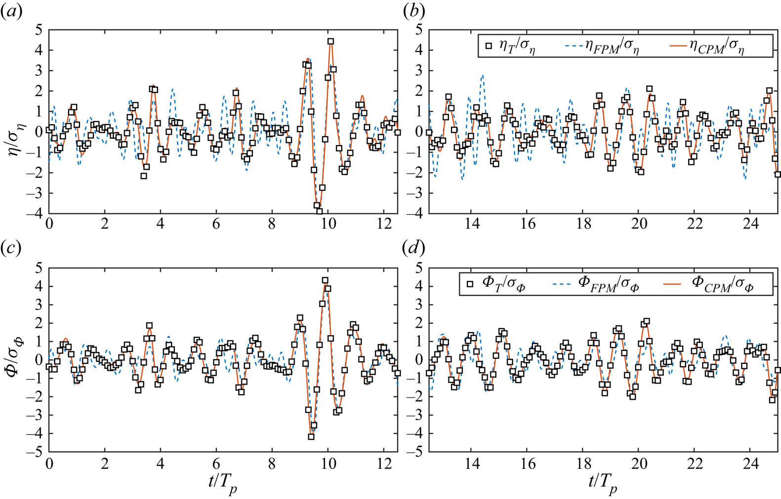
We further compare the time history of the reconstructed and predicted wave fields with the true data. Considering that the reconstructed and predicted wave field has a higher spatial resolution than the measurement (see table 3), we have first examined locations where the synthetic surface elevation measurement data are available (not plotted due to space limit): the FPM generally produces a slightly worse result compared with the CPM. As a comparison, we plot in figure 7 the results obtained using both methods at a fixed location without the measurement data ( $x=9.4\lambda _p,y=8\lambda _p$). The reconstructed surface elevation obtained by FPM has notable deviations from the true wave state, and the surface velocity potential obtained by FPM shares a similar distribution with the ground truth but with a visible difference, while the results obtained by CPM agree well with the true values. In addition, we also compare the spatial distribution of the reconstructed wave field and the true wave field along the line $y=8\lambda _p$ at $t=24$ s and $t=72$ s in figure 8. As shown in figures 8(a) and 8(b), the reconstructed surface elevation using FPM contains non-physical high-wavenumber oscillations in the spatial domain. The velocity potential obtained by FPM has a noticeable difference compared to the true data $\varPhi _T$ as shown in figures 8(c) and 8(d), which would result in a more significant difference in velocity as shown in figures 6(c) and 6(d) considering the fact that the velocity is related to the spatial derivative of the velocity potential. Similar to figure 7, CPM produces more accurate results compared to FPM. We also observed that, for the results computed at other locations (not plotted), the CPM always outperforms FPM. In summary, including a constraint between $\varPhi _0$ and the independent control variable $\eta _0$ in CPM provides an apparent improvement over FPM in recovering the true wave dynamics in both the reconstruction and prediction time duration.
Time history of the normalised surface elevation and the velocity potential located at  $(x=9.4\lambda _p,y=8\lambda _p)$ in (a,c) the reconstruction time duration ( $t<50$ s) and (b,d) the prediction time duration ( $t>50$ s). Here the subscript ‘T’ denotes the true wave data, while the subscripts ‘FPM’ and ‘CPM’ denote the methods used for reconstruction and prediction. The root mean square of the initial true surface elevation and velocity potential are $\sigma _\eta =0.18$ $m$ and $\sigma _\varPhi =1.04$ m $^{2}$ s $^{-1}$, respectively.
Instantaneous spatial distribution of the wave field along a horizontal line at  $y=8\lambda _p$ in (a,c) the reconstruction time duration ( $t=24$ s) and (b,d) the prediction time duration ( $t=72$ s). Here, the meanings of the legends are the same as those in figure 7.

3.2.2 Wave statistics
To evaluate the statistics of the reconstructed wave field, we calculate the probability density function (p.d.f.) of the wave field. In figure 9, we plot the p.d.f. of  $\eta /\langle \eta ^{2} \rangle ^{1/2}$ and $\varPhi /\langle \varPhi ^{2}\rangle ^{1/2}$ at $t=0$, $t=24$ s for the reconstructed wave field, and $t=72$ s for the predicted wave field, where the bracket $\langle {\cdots }\rangle$ denotes the spatial mean. Under the linear wave assumptions, the p.d.f. of the surface elevation yields a Gaussian distribution. However, as observed in field measurements (see e.g. Reference Ochi and WangOchi & Wang, 1985), if the wave slopes are not small, the p.d.f. deviates from the Gaussian due to the nonlinearity, which is consistent with the p.d.f. of $\eta _T$ and $\varPhi _T$ in our result. The reconstructed and predicted wave fields obtained by CPM successfully recover the p.d.f. of the true wave field, while the results by FPM have a non-negligible deviation, indicating the difference of $\eta _{\mathit {FPM}}$ and $\varPhi _{\mathit {FPM}}$ from the true values, consistent with the results in the preceding section.
Probability density function of the normalised reconstructed wave fields obtained using FPM and CPM, and the true wave field at (a,d)  $t=0$; (b,e) $t=24$ s (in reconstruction time duration); and (c, f) $t=72$ s (in prediction time duration). The standard Gaussian distribution is also plotted.

Skewness and kurtosis are important statistics to reflect the physical features of a nonlinear wave field. Specifically, the skewness measures the deviation of the wave profile from a sinusoidal shape, and the kurtosis indicates the probability of the occurrence of extreme waves (Reference Xiao, Liu, Wu and YueXiao, Liu, Wu, & Yue, 2013). We compute the skewness  $C_3$ and the kurtosis $C_4$ from the instantaneous surface elevation as
 \begin{equation} C_3=\frac{\langle \eta^3 \rangle}{\langle \eta^2\rangle^{3/2}}\quad\text{and}\quad C_4=\frac{\langle \eta^4 \rangle}{\langle \eta^2 \rangle^{2}}.\end{equation}
We present the evolution of skewness and kurtosis of the reconstructed wave field and the true wave field in figure 10. For a standard Gaussian distribution, their values are  $C_3=0$ and $C_4=3$, respectively. The skewness of the computed wave field varies from 0.05 to 0.2 and the kurtosis varies from 2.8 to 3.3, mostly above 3, which differs from the statistics of a standard Gaussian distribution because of the wave nonlinearity. As shown in figure 10, our CPM can successfully recover the skewness and kurtosis of the wave field in both the reconstruction time duration and the prediction time duration. On the other hand, there exists a distinct difference between the FPM results and the ground truth, especially for the kurtosis (see e.g. $t/T_p=11$ in figure 10b).
Evolution of (a) the skewness and (b) the kurtosis of the reconstructed wave field, i.e.  $\eta _{\mathit {FPM}}$ and $\eta _{\mathit {CPM}}$, and the true wave field $\eta _T$.

3.3 Effect of nonlinearity and measurement noise
To evaluate the effect of wave field nonlinearity and measurement noise, we perform the data assimilation for the reconstruction and prediction for wave fields with different nonlinearity and noise levels, as shown in table 2. The wave data generation process is described in § 3.1. We present the omnidirectional wavenumber spectra of the reconstructed initial wave field and the true wave field in figures 11 and 12 for the cases with the largest wave steepness and noise level, i.e. cases KA013-N00 and KA009-N10, respectively. Compared with the results for the case KA09-N00 (see figure 6), the deviation of the wave surface elevation obtained by CPM from the true wave data increases in the high-wavenumber range due to the high nonlinearity and noise. Nevertheless, the performance of CPM in reconstructing/predicting the surface elevation is much better than that of FPM.
Same legend as in figure 6. The results for the strong nonlinear case KA13-N00 are plotted.

Same legend as in figure 6. The results for the case with 10 % noise KA09-N10 are plotted.

To quantify the overall performance of CPM and FPM, we define the correlation coefficient between  $\eta$ and $\eta _T$ as
 \begin{equation} \rho(\eta,\eta_T) = \frac{\displaystyle\sum_{i=1}^{N_X}\sum_{j=1}^{N_Y} (\eta(x_i,y_j)-\langle\eta\rangle)(\eta_{T}(x_i,y_j)-\langle\eta_{T}\rangle)} {\displaystyle\sqrt{\sum_{i=1}^{N_X}\sum_{j=1}^{N_Y}(\eta(x_i,y_j)-\langle\eta\rangle)^2\sum_{i=1}^{N_X}\sum_{j=1}^{N_Y}(\eta_{T}(x_i,y_j)-\langle\eta_{T}\rangle)^2}},\end{equation}
where  $N_X$ and $N_Y$ denote the grid numbers of the reconstructed and predicted wave field in the $x$ and $y$ coordinates, respectively. The value of $\rho (\eta,\eta _T)$ is a measure of the accuracy of the data assimilation scheme, and a larger value corresponds to a better accuracy. When $\eta =\eta _T$, $\rho (\eta,\eta _T)=1$. For the surface velocity potential, the correlation coefficient is calculated using the same definition as in the above equation.
The time-averaged correlation coefficient in the reconstruction time duration ( $t<50$ s) and the prediction time duration ( $t>50$ s) for wave fields with different wave steepness and noise level are presented in figures 13 and 14. For the FPM result, the time-averaged correlation coefficients $\overline {\rho (\eta _R,\eta _T)}$ and $\overline {\rho (\varPhi _R,\varPhi _T)}$ in the reconstruction time duration decrease from 0.8 to 0.6 and from 0.9 to 0.7, respectively, with increasing wave steepness, and the correlation coefficients in the prediction time duration decrease from the values in the reconstruction time duration more rapidly with higher wave steepness. For the CPM result, the correlation coefficient of the reconstructed wave field with the true wave field is above 0.9 for all the cases. Figure 14 shows that the effect of noise level in the range of 0 % to 10 % has a negligible effect on the reconstruction performance. In these cases, the correlation coefficients of the reconstructed and predicted wave field obtained by CPM are notably higher than those obtained by FPM. Therefore, the advantages of CPM over FPM are unaffected by the measurement noise and higher wave nonlinearity. Simulations with different initial random wave phases are also performed for cases KA09-N00, KA09-N10 and KA13-N00. As shown in table 4, we found that the wave reconstruction and prediction performance for both FPM and CPM, quantified by correlation coefficients, varies only slightly with the initial random wave phases.
Time-averaged correlation coefficients of the reconstructed and predicted (a) surface elevation and (b) velocity potential with the true wave data. The subscripts ‘R’ and ‘P’ denote the reconstruction and prediction time duration, respectively. The results for cases KA03-N00, KA06-N00, KA09-N00 and KA13-N00 are plotted.

Same legend as in figure 13. The results for cases KA09-N00, KA09-N03, KA09-N06 and KA09-N10 are plotted.

Correlation coefficients for different sets of initial random wave phases.

4. Discussion
4.1 Reasons for better performance of CPM
The better performance in CPM over FPM is likely due to three factors. First, the non-physical high-wavenumber wave components have been removed by using the wave-physics-based constraint for control variables in CPM. The wave model, i.e. (2.1) and (2.2), only restricts the evolution of  $\eta$ and $\varPhi$. However, $\eta _0$ and $\varPhi _0$ are independent variables that serve as the initial condition (Reference ZakharovZakharov, 1968). In wave simulations, appropriate initial states are required to ensure that the wave dynamics are captured correctly. In FPM, the initial wave states are obtained via a gradient-based optimiser that does not guarantee the physical reasonableness of the found solutions for this complex system and results in a solution with non-physical high-wavenumber waves. The additional constraint in CPM, on the other hand, helps the optimisation algorithm to search for a solution with the reasonable initial wave state quantified by $\eta _0$. If the nonlinearity were to be included in the dispersion relation, the frequency of a given wave would be a function not only of the wavenumber and amplitude of itself but also of those of all other free-wave components (Reference WuWu, 2004). Therefore, it is infeasible to write a similar formula to serve as the constraint. Besides, because this linear assumption is imposed only at the initial time, and the forward wave model captures the nonlinear evolution afterwards, we do not expect a significant change in the reconstructed and predicted wave field even if a nonlinear dispersion relation can be incorporated into the constraint between $\eta _0$ and $\varPhi _0$.
Second, the additional constraint in CPM addresses the issue of the inhomogeneity in the magnitude of the gradient in the optimisation process of FPM. In the gradient-based optimisation used in FPM, the increment of the control parameters is proportional to the gradient magnitudes, and thus the optimiser tends to modify the parameters with large gradients, i.e.  $\eta _0$. However, in CPM, the control parameter $\varPhi _0$ is connected to $\eta _0$, which would not have the same problem caused by the different order of gradient magnitudes. An alternative way to examine this issue is to use the scaling strategy. Strictly speaking, the suitable value for scaling is unknown before wave reconstruction because the velocity potential is unknown and only sparse measurements of surface elevation are available. However, for the sake of the performance testing, we assume $\sigma _\eta$ and $\sigma _{\varPhi }$ are known and choose them as the scaling factors for $\eta$ and $\varPhi$, respectively, to ensure that the normalised variables have the same order of magnitude. As shown in table 5, while the scaling strategy enhances the performance of FPM, its cost function is still 60 times larger than that in CPM, suggesting that the performance issue in FPM cannot be solved by scaling.
Effect of scaling of control variables on the cost function for case KA09-N00. Listed are the convergence values of the cost function normalised by the initial value.

Third, this seemingly counter-intuitive worse performance in FPM by using an extra control variable  $\varPhi _0$ is known as the degradation problem widely observed in the optimisation of complex systems with large degrees of freedom (Reference He, Zhang, Ren and SunHe, Zhang, Ren, & Sun, 2016). Specifically, when the number of independent control variables increases, the performance of the optimiser decreases counter-intuitively such that the optimiser fails to find the global optimal solution. The degradation problem is based on the observation of an abnormal increase of the cost function with adding more free control variables. Rigorous theoretical explanation is still a research topic to address in the research community. An effective method that has been adopted by the deep neural network optimisation community to alleviate the degradation problem is to add connections in different neural layers to change the system structure. Our results show that a wave-physics-based constraint introduced in the CPM can also provide an effective solution to help the optimiser when searching for the globally optimal result.
4.2 Effect of the discretisation of measurement on CPM performance
We have shown that measurement with a coarse resolution of  $\Delta x_M/\lambda _p = 0.5$ and $\Delta t_M/T_p=0.1$ is sufficient to accurately capture the high-frequency information at the present configuration using CPM. Theoretically, by assuming that the temporal resolution of the measurement is adequately high and by using the linearised wave theory, it is possible to determine the predictable zone for irregular wave fields by the maximum and minimum wave group velocities and direction spreading angle of the wave field as well as the spatial and temporal extents of the measurement (Reference Qi, Wu, Liu and YueQi, Wu, Liu, & Yue, 2018; Reference WuWu, 2004). However, this theoretical work is inapplicable for discretised spatial and temporal resolutions, which are typically seen in wave measurement practice. For the case KA09-N00, CPM has a fairly good performance in the reconstructed surface elevation spectrum when the temporal resolution is changed to $\Delta t_M/T_p =0.2$, as shown in figure 15(a). However, the performance declines significantly when the resolution is $\Delta t_M /T_p = 0.3$.
Omnidirectional wavenumber spectra of the reconstructed initial surface elevation using measurements of different temporal resolutions and the true initial surface elevation: (a) for case KA09-N00; and (b) for a typical wave field of wave period  $T_p =10$ s. Results are obtained using CPM.

We also test the reconstruction performance for another wave field with  $\lambda _p=156$ m, $T_p=10$ s, $(ka)_e=0.08$ and $(ka)_l=0.33$ as shown in figure 15(b). The simulation time step $\Delta t =0.25$ s and the domain length is $16\lambda _p \times 16 \lambda _p$ with the $512 \times 512$ grid resolution. Two simulations are conducted with this wave field with measurements of different temporal discretisation $\Delta t_M/T_p =0.125$ and $\Delta t_M/T_p =0.25$ and the same spatial resolution $\Delta x_M/\lambda _p = 0.5$. Similar to the result shown above, high-wavenumber wave components are observed with $\Delta t_M/T_p =0.25$, while CPM obtains good reconstruction performance for $\Delta t_M/T_p =0.125$. Note that for all the cases, reconstructed wave fields obtained in CPM have higher correlation coefficients with the true wave fields than the results obtained from FPM. Therefore, the discretisation of measurement is an important factor that affects the accuracy of CPM. In real applications, we need to choose appropriate combinations of the spatial and temporal resolutions of measurement to obtain satisfactory results.
5. Conclusions
In this study, we have investigated the assimilation of measurement data for the wave field reconstruction and prediction based on the HOS method and its adjoint model. In our method, we quantify the difference between the reconstructed/predicted wave field and measurement as a cost function. Compared with the conventional adjoint-based wave data assimilation method, FPM, we have introduced a physical constraint on the initial wave field in the new method, CPM, which is shown to effectively reduce the cost function in both the reconstruction and prediction. In the optimisation process, we use the L-BFGS-b method to minimise the cost function, and convergence can be reached within several iterations steps. The new method can be applied to situations where the wave measurement data have a low resolution.
To evaluate the performance of the new method, CPM, we have generated wave data with different wave steepness and noise levels. The gradient information calculated using the adjoint model is validated against that obtained from the finite-difference method (see the supplementary material). We have conducted numerical tests to examine the optimisation, reconstruction and prediction performance for the new CPM and the conventional FPM. In the test results, CPM shows an advantage over FPM. Using one half of the control variables in FPM, CPM proves to be more efficient in reducing the overall cost function than FPM. We have also calculated the omnidirectional wavenumber spectra of the optimal initial wave states. It is found that non-physical high-wavenumber components are generated in reconstructed surface elevation and the magnitude of the initial surface velocity potential is underestimated in the FPM results, while the CPM results are close to the ground truth, demonstrating an improved capability of wave field reconstruction and prediction. The time history and the spatial distribution of the wave states reconstructed and predicted by CPM show significantly smaller errors than FPM. In addition, the CPM can successfully predict key wave statistics, including the p.d.f., skewness and kurtosis of the wave field. We have also investigated the effect of measurement noise and wave nonlinearity, and observed a better performance of CPM over FPM in all cases.
Finally, we remark that in this study the performance of data assimilation is evaluated using the synthetic wave data obtained from simulation, which might be limited by the assumptions employed by the wave model, e.g. potential flow and periodic boundary conditions. In applications, similar tests can be conducted using wave data with realistic noise obtained from field measurements. Other effects, such as bottom topology, ambient current, wind forcing and wave breaking, are not incorporated in the present wave model but could in principle also be included with modifications (Reference WuWu, 2004). When a physical process is significant but not captured in a wave model, the error caused by the model inaccuracy would result in an inaccurate reconstructed wave field. In future studies, it would be interesting to incorporate these effects in a modified data assimilation framework for both the wave model and the adjoint model.
Acknowledgements
The authors would like to thank the anonymous reviewers for their helpful comments.
Funding Statement
The work is supported by the Office of Naval Research and University of Minnesota Sea Grant.
Declaration of Interests
The authors declare no conflict of interest.
Data Availability Statement
Raw data are available from the corresponding author (L.S.).
Ethical Standards
The research meets all ethical guidelines, including adherence to the legal requirements of the study country.
Supplementary Material
Supplementary information is available at https://doi.org/10.1017/flo.2021.19.


 Open access