

1. Introduction
In a “temperate” glacier, as usually defined, all the ice is at the pressure melting point except for a near-surface layer, some 10 m thick, whose temperature is below 0° C in winter (Reference AhlmannAhlmann, 1935). The name arises because such glaciers are found mainly in temperate regions; but not all glaciers in these regions are of this type. For example, sub-freezing temperatures have been measured, at depths below the limit of seasonal variations, in the ice cap at the Jungfraujoch and on Mont Blanc, Breithorn and Monte Rosa in the Alps (Reference VallotVallot, 1913; Reference Hughes and SeligmanHughes and Seligman, 1939; Reference FisherFisher, 1955, Reference Fisher1963), in Vesl-Skautbreen in Norway (Reference McCallMcCall, 1952), in Lednik Tsentral’nyy Tuyuksu in the Tien Shan, U.S.S.R. (Reference VilesovVilesov, 1961), in Taku Glacier in southern Alaska (Reference MillerMiller, [1956]), and at the base of South Leduc Glacier in western Canada (Reference MathewsMathews, 1964). Again, Reference SchyltSchytt (1968) measured temperatures below 0° C in Stor Glaciären in Swedish Lappland which, though north of the Arctic circle, had previously been considered temperate. How widespread temperate glaciers are thus remains uncertain.
For a glacier to be temperate, the whole of the layer that is cooled in winter must be brought to 0° C during the following summer. In the accumulation area, heat transfer from the surface to the underlying firn has been studied in detail by Reference SverdrupSverdrup (1935), Reference Hughes and SeligmanHughes and Seligman (1939), Reference SharpSharp (1951), and others. They found that, once surface melting begins, the dominant factor in warming the firn is latent heat released when percolating melt water refreezes on contact with a sub-freezing layer. In the ablation area, however, latent heat is much less important because ice is, at best, only slightly permeable to water. As a result, ice may be warmer in the accumulation area than in the ablation area. Reference PatersonPaterson (1969, p. 175) has quoted some examples of this. In particular, some glaciers may be temperate only in the accumulation area (Reference LoeweLoewe, 1966; Reference SchyltSchytt, 1968, Reference Schytt1969).
In comparison with the detailed studies made in the accumulation area, heat transfer from the surface to the underlying layers in the ablation area seems to have received less attention. A discussion of this question, based on data from Athabasca Glacier, forms the subject of this paper.
2. Athabasca Glacier
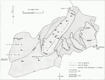
Athabasca Glacier (lat. 52.2° N., long. 117.2° W.) is one of the main outlet glaciers from the Columbia Icefield in the Canadian Rocky Mountains. The Icefield lies on the continental divide some 700 km from the Pacific Ocean. Table I contains data for the two nearest weather stations. Figure 1 shows the glacier; Reference Paterson and SavagePaterson and Savage (1963) have described it in detail. The equilibrium line usually lies at an elevation of about 2 600 m in the highest of three ice falls by which the glacier descends from the Icefield. Snow pits, dug in the ablation area in late April, reveal no sign of melting during the winter and indicate that the winter precipitation is equivalent to roughly 1 m of water. In most years, the entire snow cover in the region, 3.8 km long, between the foot of the lowest ice fall and the terminus reaches a temperature of 0° C in late June; the ice becomes free of snow in the first half of July and the ablation season ends in the first half of September. About 3.8 m of ice is lost annually from this section; the amount varies little from place to place except near the terminus and in moraine-covered areas near the valley walls.
Map of Athabasca Glacier showing locations of 10-meter bore holes.
Climatic Data for the Two Stations Nearest to Athabasca Glacier

3. Temperature measurements
Temperatures were measured by thermistors in holes, 10 m deep, made with a hand drill. Resistance was measured to the nearest 10 Ω which corresponds to 0.04 deg. Figure 1 shows the positions of the holes. Table II lists 10-meter temperatures in all holes except hole F which punctured a water-filled cavity at a depth of 9.2 m (Reference Paterson and SavagePaterson and Savage, 1970), hole J into which water penetrated from the surface, and hole K which was only 5.2 m deep. In some holes, temperatures were measured at various depths down to 10 m. Figure 2 shows temperatures in late April 1968, about the time of maximum winter cooling. Figure 3 shows temperatures in September 1970 at the end of an exceptionally heavy ablation season (about 5 m compared with an average of 3.8 m); ablation had ended by then, air temperature was below 0° C and there was up to 0.5 m of fresh snow on the glacier. We defer discussion of these observations until we have considered the ways in which ice below the surface may receive heat in summer.
Snow and ice temperatures measured in three bore holes in late April 1968, and regression line (Equation (3)) fitted to the ice temperatures. The top point in each hole was at the surface.

Ice temperatures measured in three bore holes on 22 September 1970.

Ten-Meter Temperatures In Athabasca Glacier
(Holes A, B, C are in accumulation area, others in ablation area)

4. Conduction and ablation
An appropriate mathematical model is that of heat conduction in a moving semi-infinite medium. To consider a slab of finite thickness would be preferable, but for this case the equation has no analytical solution. Reference BenfieldBenfield (1951, Reference Benfield1953) has used the same model to study how accumulation affects temperatures in a snowfield.
Let T denote temperature, t time, y depth below surface and k thermal diffusivity. The region y > 0 moves with velocity v, negative for the case of ablation because ice moves upwards relative to the surface. The initial temperature is T 0+ay. From t = 0 (the start of the ablation season) the surface y = 0 is maintained at T = 0.
The equation of heat transfer is
The solution is a special case of that given by Reference Carslaw and JaegerCarslaw and Jaeger (1959, p. 388):

Here

We use this solution to determine temperature as a function of depth at the end of the ablation season. We take the regression line fitted to the April measurements (Fig. 2)
to represent temperature at t = 0. Curve (c) in Figure 4 shows the solution of Equation (2) with numerical values appropriate to Athabasca Glacier: T = −4.23° C, a = 0.38 deg m−1, length of ablation season t = 0.2 a, total ablation vt = −3.8 m, k = 36.3 m2 a−1. It appears that, even when allowance is made for the ice removed by ablation, heat conduction is inadequate to warm all the ice to 0° C by the end of the ablation season. Thereafter, there is a net loss of heat from the surface so all the ice will never reach 0° C.
Temperature profiles calculated from heat-conduction theory.
-
(a) Observed initial temperatures (see Fig. 2).
-
(b) Temperatures after 0.2 a with no ablation.
-
(c) After 3.8 m ablation in 0.2 a (average conditions in Athabasca Glacier).
-
(d) After 3.8 m ablation in 0.4 a.
-
(e) After 7.5 m ablation in 0.2 a.

Figure 4 includes curves for three additional cases to show the effect of variations in ablation rate and in length of ablation season; the variations are larger than those encountered from year to year on Athabasca Glacier. The curves illustrate the importance of the amount of ablation in determining the temperature distribution. The curves are easily converted to “cold waves” of different amplitudes; if T 0 and a are each multiplied by m, the final temperatures are also.
5. Percolation and refreezing of melt water
Reference Nye and FrankNye and Frank (in press) believe that, contrary to previous opinions (Reference SteinemannSteinemann, 1958; Reference LliboutryLliboutry, 1964–5, Tom. 1, p. 112–3), pure polycrystalline ice at the melting point is permeable to water. Thus latent heat, released by percolating melt water when it refreezes on contact with a subfreezing layer, is a possible means of warming the ice in the ablation area. We now try to assess its importance.
On Nye and Frank’s model (c.f. Reference FrankFrank, 1968), the ice is assumed to be at the pressure melting point throughout and the water flows downwards, under a pressure gradient due to the density difference between ice and water, through a network of veins between the ice grains. The situation considered here is somewhat different. At the end of summer, when the supply of melt water is cut off and the ice starts to lose heat, any water in the near-surface ice will freeze and ice creep will start to close any air-filled veins or cavities. Thus, by the beginning of the following summer, the permeability of the near-surface ice should be almost zero. Thus, at each depth, melt water will have to penetrate from the surface, freeze and release latent heat to bring the surrounding ice to the melting point and open up channels, before water can proceed to greater depths. As the details of this process are not clear, we propose to treat it as a process of diffusion of water into a semi-infinite medium. At each depth, the water must reach a certain concentration before it can advance further; the concentration is such that the latent, heat released by the water on freezing is just sufficient to warm the ice at that depth to 0° C. We assume that the concentration of water at the surface remains constant and that its temperature is 0° C. Reference HillHill (1928) has used the same mathematical model in another problem.
Let y denote distance below the surface, t time, f(y, t) volume of water per unit volume of ice, and λ the volume concentration of water needed to raise the ice at depth y to 0° C. Thus λ = ρcΔT/ρ′L where ρ and ρ′ are densities of ice and water, c specific heat of ice, L its latent heat, and ΔT difference between ice temperature and 0° C. Initially, ΔT and thus λ are assumed to be the same at all depths. Let Y(t) be the depth to which water has penetrated (the position of the 0° C isotherm) at time t. We wish to determine Y(t) as a function of λ and of f 0, the value of f at the surface.
The diffusion equation is
where k is the diffusivity of water in ice. By using this equation we assume that the pressure gradient that makes the water flow downwards is not the dominant factor in determining the rate of penetration and therefore can be neglected. In addition, we assume that k is constant above the 0° C isotherm and that f 0, the water concentration at the surface, is constant in time. These are dubious assumptions.
Boundary conditions are:
At
For
At
At y =Y(t), the rate of diffusion of water must be equal to the rate at which water is being used to warm the ice. Thus
The solution of Equation (4) satisfying Conditions (5) and (6) is
Condition (7) then gives
where, from Condition (8), B is given by
The value of B, for given f 0 and λ, can be determined from a table of B erf B exp B 2.
From Equation (9) one can calculate whether the water has reached the lower boundary of the cold layer by the end of the ablation season, when the surface water supply is cut off. The data required are λ, f 0, and k. From Equation (3), and appropriate values of the density and specific and latent heats of ice,
We take f 0 = 0.01. This is probably an upper limit. Reference Nye and FrankNye and Frank (in press) consider that f is unlikely to exceed 0.001. Reference JoubertJoubert (1963) measured values from 0.0015 to 0.01 in ice in the Vallée Blanche, Reference AmbachAmbach (1956) measured values up to 0.03 in Vernagtferner, but that was in ice within 160 mm of the surface where there is probably more water than at depth. Moreover, these measurements would include any water in isolated cavities as well as that in the vein system. There appear to exist no data on which to base an estimate of k for ice. However, a value for firn can be obtained from the data of Reference Hughes and SeligmanHughes and Seligman (1939) who measured both temperatures and water percolation in the Jungfraufirn as functions of time. Application of the above theory to their data gives k = 185 m2 a−1. For ice, it seems plausible to reduce this value by at least one order of magnitude and take k = 20 m2 a−1.
With the above values, Equation (9) becomes
For Y = 10 m (minimum thickness of cold layer), t = 4.5 a. For t = 0.2 a (length of ablation season), Y = 2.1 m. A slightly more complex analysis in which λ is allowed to vary linearly with depth gives similar values: for Y = 10 m, t = 2.6 a and for t = 0.2 a, Y = 2.1 m. Thus the rate of melt-water penetration is less than the ablation rate. We conclude that refreezing of percolating melt water should be a negligible factor in warming the ice in the ablation area of Athabasca Glacier.
The foregoing theory is obviously much more elaborate than is warranted by existing data. The percolation of water through glacier ice needs detailed study.
6. Solar radiation
Reference LliboutryLliboutry (1964–5, Tom. 1, p. 368) gives values of the extinction coefficient for solar radiation in glacier ice: 0.028 mm−1 at the surface, decreasing to 0.0018 mm−1 at depths below 0.2 m. These figures imply that 50% of solar radiation is absorbed in the uppermost 30 mm and 99% in the first 1.85 m. In this case, solar radiation may be neglected as a means of warming the ice below the surface, although it is of course often the major factor in warming and melting the surface ice. However, Reference WellerWeller (1968) measured extinction coefficients of only 0.0013 mm−1 down to 1 m and 0.0007 mm−1 below that depth in Antarctic “blue ice” and concluded that radiation was an important means of heat transfer even at a depth of 4 m. Lliboutry’s data appear to refer to conditions in the Alps in the ablation season and are therefore more appropriate for Athabasca Glacier than Weller’s data from a region where the surface temperature was always below 0° C. We conclude that solar radiation can probably be neglected in the case of Athabasca Glacier; but some measurements would be desirable.
7. Discussion of measured temperatures
Table II indicates that, on the plausible assumption that winter cooling does not penetrate below 10 m, the glacier is temperate in the accumulation area. Figure 3 shows that, in the ablation area, the ice had not attained the pressure melting temperature by the end of what was an exceptionally heavy ablation season. If the melting point has not been reached by the end of summer it never will be, because the ice then starts to lose heat again to the atmosphere. The data in Table II confirm that the ablation area is not temperate; all the 10-meter temperatures there, measured in three different years and at different times of year, are below 0° C. Whether, at a given point, there are any measurable seasonal variations in 10-meter temperature is not known because thermistors were not left in the ice; fresh holes were drilled, usually at different locations, on each visit to the glacier. However, the 10-meter temperatures in holes E and H in April were close to that in hole G, which is at about the same elevation, in the previous August. During the ablation season, because the surface level is changing, one might expect slight differences between temperatures measured at a depth of 10 m at different times.
If hole L is excluded, the data in Table II show a slight trend for 10-meter temperature in the ablation area to decrease with increase of elevation (rate of about 0.3 deg per 100 m). Hole L was in moraine-covered ice near the valley walls. Hole K. was also, and measurements there confirm that temperatures in this type of ice are lower than in the relatively clean ice in the central part of the glacier. Hole K only penetrated to 5.2 m but the temperatures there was − 1.9° C, the same as at that depth in hole L. Ablation of the moraine-covered ice is only about 60% of that elsewhere. Figure 4 illustrates how a decrease in the amount of ablation results in lower temperatures at depth. We suggest that this is the explanation of the observations. A contributing factor may be that, because the moraine-covered ice stands relatively high, some snow may be removed by wind. Thus the accumulation there may be relatively low. This would increase the winter heat loss.
The observations thus confirm the conclusion, drawn from the preceding sections, that insufficient heat is supplied to the ice below the surface to bring it all to the melting point by the end of summer. The temperature profiles measured in September (Fig. 3) resemble those calculated from heat conduction theory (Fig. 4). Close quantitative agreement between theory and observation can hardly be expected, because the initial temperatures (Fig. 2) used in the calculations were measured at different places and in a different year from the final ones (Fig. 3). Moreover, the regression line is only a rough representation of the initial temperature. Perhaps the major discrepancy between Figures 3 and 4 is in the depth of minimum temperature. However, calculations show that the position of the minimum depends quite sensitively on the choice of initial temperature. We believe that inaccuracies in this can explain the discrepancy.
If penetration of melt water and solar radiation were significant means of heat transfer, the temperatures at the end of summer might still be calculated from heat-conduction theory, provided that a larger-than-normal value of thermal diffusivity were used. If increasing the value of diffusivity improved significantly the fit of the theoretical curves to the observations, this would suggest that the additional heat sources are not negligible. However, the limitations of the present data, mentioned above, preclude such a test.
8. Discussion: conditions for temperate ablation area
Whether the near-surface layers in a glacier attain a temperature of 0° C by the end of summer depends both on the winter heat loss and the summer heat supply. The heat loss depends on such factors as winter air temperatures, extent of cloud cover, amount of snowfall and when it occurs. The preceding analyses indicate that ablation is the main factor in eliminating the winter “cold wave” in the ablation area. In other words, the heat that the surface receives from the atmosphere and from solar radiation is largely used to warm the surface ice to 0° C and then melt it. The sub-surface ice receives some heat by conduction. The longer the ablation season, the more effective conduction will be; but the amount of heat supplied in a typical season of two or three months is not large. (See Fig. 4.)
Thus we may speculate that few, if any glaciers are temperate throughout. Many glaciers appear to be temperate in the accumulation area. However most of these probably contain a region below the equilibrium line where, because ablation is small, some of the ice cooled in winter remains below the melting point throughout the following summer. In some glaciers this region of cold ice may extend to the terminus; in others, ablation at lower elevations may be sufficient to make the glacier temperate there. The critical value of ablation will of course depend on the extent of winter cooling.
Reference SchyttSchytt (1969) has described this situation in Svalbard: “In many glaciers, previously considered as temperate, … the cooling starts just above the equilibrium line and the ice temperature in the upper several tens of meters stays below 0° C all the way to the ice edge”. Schytt’s observation that the cold ice starts “just above” the equilibrium line has not been checked on Athabasca Glacier because the equilibrium line lies in an ice fall. However, hole C, where the temperature is 0° C, is a horizontal distance of only 600 m above the equilibrium line.
Reference VilesovVilesov (1961) measured temperatures at different times of year in the ablation area of Lednik Tsentral’nyy Tuyuksu in the Tien Shan. In comparison with Athabasca Glacier, the winter cooling is greater (1-meter temperature of −6° C compared with −4° C) and ablation is less (2 m a−1 against 3.8 m a−1), although the ablation season is about the same length on both glaciers; thus the 10 m temperature is lower (− 2.5° C against −0.5° C)
Let us consider some other regions. In the European Alps, ablation exceeds 10 m a−1 on the lower parts of major glaciers such as Grosser Aletschgletscher (Reference KasserKasser, [1956]) and Mer de Glace (Reference LliboutryLliboutry and others, 1962). But ice below the melting point might be found in she higher parts of the ablation areas of these glaciers, or in small glaciers whose termini are at relatively high elevations where ablation may be only 2 or 3 m a−1. Blue Glacier, in north-western U.S.A., is temperate in the accumulation area; the temperature in the ablation area has not been measured (Reference Shreve and SharpShreve and Sharp, 1970). As the maximum ablation is only 3.5 m a−1 (Reference LaChapelleLaChapelle, 1965), one might expect that the ablation area would not be temperate. However, Reference LaChapelleLaChapelle (1961) found that, as a result of mild winters and heavy snowfalls, the temperature of the firn in the accumulation area hardly ever falls below −2° C and that sub-freezing temperatures never penetrate below 4 m. Conditions are probably similar in the ablation area. Moreover, the ablation season lasts 4 months, a relatively long period (Reference LaChapelleLaChapelle, 1965). In these circumstances, at least the lower part of the ablation area should be temperate.
The preceding discussion is oversimplified. Because accumulation and ablation vary over short distances as a result of variations in the nature and topography of the surface, thermal conditions will also vary. Figure 2, for example, illustrates how snow depth affects ice temperature. Again, the ice in the bed of a melt-water stream may be maintained at 0° C throughout the summer, while ice on the crest of a hummock may be cooled by radiation every night; crevasses, moulins and melt streams influence the temperature of the surrounding ice; significant amounts of solar radiation may penetrate patches of bubblefree ice. Heat conduction will reduce such temperature inhomogeneities, but is unlikely to eliminate them. Perhaps, in some glaciers, conditions resemble those in regions of discontinuous permafrost, where patches of ground that thaw during summer are interspersed with patches that remain frozen. Moreover, ice temperature may vary from year to year as a result of climatic fluctuations. While seasonal variations are negligible at depths below about 10 m, changes with longer periods are propagated to greater depths.
This paper, if it has done nothing else, should have pointed out the need for more temperature measurements in glaciers in temperate regions and also for detailed studies of the penetration of water and solar radiation into glacier ice.
9. Acknowledgements
Drs J. C. Savage and R. M. Koerner and Messrs C. S. L. Ommanney and D. Halyko helped in different stages of the field work. Mr W. Ruddy of Snowmobile Tours Ltd, Jasper, Alberta kindly provided transport of equipment on the glacier and also assisted in other ways.
Note. This paper was submitted before the publication of an important paper on the same general topic by Reference LliboutryLliboutry (1971).


