2 THE NEW DYNAMICAL MODEL

Our total analytical gravitational 3D potential Φ(x, y, z) consists of three main components: a central spherical component Φ_n, a flat disk Φ_d, and a bar potential Φ_b. We decided to include only these three components, so as to be able to directly relate our results with those of the corresponding three component model presented in Pfenniger (Reference Pfenniger1984).

For the description of the spherically symmetric nucleus, we use a Plummer potential (Binney & Tremaine Reference Binney and Tremaine2008)

(1) $$\begin{equation} \Phi _{\rm n}(x,y,z) = - \frac{G M_{\rm n}}{\sqrt{x^2 + y^2 + z^ 2 + c_{\rm n}^2}}, \end{equation}$$

where G is the gravitational constant, while M _n and c _n are the mass and the scale length of the nucleus, respectively. At this point, we must point out that potential (1) is not intended to represent a black hole nor any other compact object, but a dense and massive bulge (nucleus). Therefore, we do not include any relativistic effects.

The flat disk is modelled by a Miyamoto-Nagai potential (Miyamoto & Nagai Reference Miyamoto and Nagai1975)

(2) $$\begin{equation} \Phi _{\rm d}(x,y,z) = - \frac{G M_{\rm d}}{\sqrt{x^2 + y^2 + \left(k + \sqrt{h^2 + z^ 2}\right)^2}}, \end{equation}$$

where M _d is the mass of the disk, while k and h are the horizontal and vertical scale lengths of the disk, respectively.

In order to model the properties of the galactic bar, we decided to develop a new dynamical model. The basic idea is to construct a bar from a mass distribution of length 2a which lies along the x-axis and has a continuum of centres going from x = −a to x = +a. We call this interval lying in the 3D position space I_B. The total mass of the bar is M _b. We imagine that in a first step, we have a mass distribution along I_B with a constant linear mass density m = M _b/2a. To avoid all problems with singularities of point densities and in order to include the transverse width c _b of the bar, we imagine that in a second step the linear density m belonging to a single point of I_B is smeared out over the effective width c _b. Thereby each point s from the interval I_B becomes the centre of the regularised monopole potential of the form

(3) $$\begin{equation} v(x-s,y,z) = - \frac{G m}{ \sqrt{(x-s)^2 + d^2}}, \end{equation}$$

where

(4) $$\begin{equation} d^2 = y^2 + z^2 + c_b^2 \end{equation}$$

and the total potential Φ_b(x, y, z) becomes the integral of these contributions over the interval I_B, i.e.,

(5) $$\begin{eqnarray} \Phi _{\rm b}(x,y,z) &=& \int ^{+a}_{-a} ds \; \; v(x-s,y,z)\nonumber\\ &=& \frac{G M_{\rm b}}{2a}\left[ \text{arcsin}h \left( \frac{x-a}{d} \right) - \text{arcsin}h \left( \frac{x+a}{d} \right) \right]\nonumber\\ &=& \frac{G M_{\rm b}}{2a} \ln \left( \frac{x-a+\sqrt{(x-a)^2 + d^2}}{x+a+\sqrt{(x+a)^2 + d^2}} \right). \end{eqnarray}$$

As always, we recover the corresponding mass density ρ(x, y, z) from the Poisson’s equation

(6) $$\begin{eqnarray} \rho (x,y,z) &=& \frac{1}{4 \pi G} \nabla ^2 \Phi _{\rm b}(x,y,z)\nonumber\\ &=& \frac{M_{\rm b} c_{\rm b}^2}{8 \pi a} \int ^{+a}_{-a} ds ((x-s)^2 + d^2)^{-5/2}\nonumber\\ &=& \frac{M_{\rm b} c_{\rm b}^2}{8 \pi a} (g(x+a,y,z) - g(x-a,y,z)), \end{eqnarray}$$

where

(7) $$\begin{equation} g(x,y,z) = x(2x^2 + 3d^2)d^{-2}(x^2 + d^2)^{-3/2}. \end{equation}$$

Note that the integral of ρ over all space gives correctly M _b. The rotationally symmetric limit a → 0 gives correctly

(8) $$\begin{equation} \Phi _{\rm b}(x,y,z) = - \frac{G M_{\rm b}}{ \sqrt{x^2 + d^2}}, \end{equation}$$

(9) $$\begin{equation} \rho (x,y,z) = \frac{3 M_{\rm b} c_{\rm b}^2}{4 \pi } (x^2 + d^2)^{-5/2}. \end{equation}$$

The bar rotates clockwise around its z-axis at a constant angular velocity Ω_b. The major axis of the bar points into the x direction while its intermediate axis points into the y direction. Therefore, the effective potential is

(10) $$\begin{equation} \Phi _{\rm eff}(x,y,z) = \Phi (x,y,z) - \frac{1}{2}\Omega _{\rm b}^2 \left(x^2 + y^2 \right). \end{equation}$$

We use a system of galactic units, where the unit of length is 1 kpc, the unit of mass is 2.325 × 10⁷M_⊙ (solar masses) and the unit of time is 0.9778 × 10⁸ yr (about 100 Myr). The velocity unit is 10 km s⁻¹, the unit of angular momentum (per unit mass) is 10 km kpc s⁻¹, while G is equal to unity. The energy unit (per unit mass) is 100 km²s⁻², while the angle unit is 1 radian. In these units, the values of the involved parameters are: M _n = 400 (corresponding to 9.3 × 10⁹ M_⊙), c _n = 0.25, M _d = 7000 (corresponding to 1.6275 × 10¹¹ M_⊙), k = 3, h = 0.175, M _b = 3500 (corresponding to 8.13 × 10¹⁰ M_⊙), a = 10, c _b = 1, and Ω_b = 1.25. This set of the values of the parameters defines the Standard Model (SM).

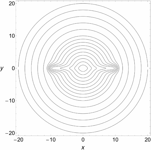
The isoline contours of constant effective potential on the (x, y)-plane for z = 0 as well as the position of the five Lagrangian points L_i,i = 1, 5 are shown in Figure 1. Three of them, L ₁, L ₂, and L ₃, known as the collinear points, are located on the x-axis. The central stationary point L ₁ at (x, y) = (0, 0) is a local minimum of Φ_eff. At the other four Lagrangian points, it is possible for the test particle to move in a circular orbit, while appearing to be stationary in the rotating frame. For this circular orbit, the centrifugal and the gravitational forces precisely balance. The stationary points L ₂ and L ₃ are saddle points, while points L ₄ and L ₅ on the other hand, are local maxima of the effective potential, enclosed by the banana-shaped isolines. The annulus bounded by the circles through L ₂, L ₃, and L ₄, L ₅ is known as the ‘region of co-rotation’. The numerical value of the effective potential at the two Lagrangian points L ₂ and L ₃ results in a critical Jacobi constant C_L = −869.70514693. Similarly, in Figure 2, we observe the isoline contours of the mass density on the (x, y)-plane for z = 0 of the total gravitational potential. The barred structure is clearly visible in the region − 10 ⩽ x ⩽ +10 kpc. Here, we should emphasise that the shape of the equidensity curves is very similar to that of the Ferrer’s ellipsoid [see e.g., Figure 1 in Pfenniger (Reference Pfenniger1984)].

Figure 1.

The isoline contours of the effective potential in the (x, y)-plane for z = 0 for the standard model. Included are the five Lagrangian points.

Figure 2.

The isoline contours of the mass density on the (x, y)-plane for z = 0 of the total gravitational potential Φ(x, y, z) for the standard model.

The motion of a test particle with a unit mass (m = 1) in our rotating barred galaxy model is governed by the Hamiltonian

(11) $$\begin{equation} H = \frac{1}{2} \left(p_x^2 + p_y^2 + p_z^2 \right) + \Phi (x,y,z) - \Omega _{\rm b} \left( x p_y - y p_x\right) = E, \end{equation}$$

where p_x, p_y, and p_z are the momenta per unit mass, conjugate to x, y, and z respectively, while E is the numerical value of the Jacobi integral, which is conserved.

(12) $$\begin{eqnarray} \dot{x} &=& p_x + \Omega _{\rm b} y, \nonumber \\ \dot{y} &=& p_y - \Omega _{\rm b} x, \nonumber \\ \dot{z} &=& p_z, \nonumber \\ \dot{p_x} &=& - \frac{\partial \Phi }{\partial x} + \Omega _{\rm b} p_y, \nonumber \\ \dot{p_y} &=& - \frac{\partial \Phi }{\partial y} - \Omega _{\rm b} p_x, \nonumber \\ \dot{p_z} &=& - \frac{\partial \Phi }{\partial z}, \end{eqnarray}$$

where the dot indicates derivative with respect to the time.

In the same vein, the variational equations which govern the evolution of a deviation vector w = (δx, δy, δz, δp_x, δp_y, δp_z) are

(13) $$\begin{eqnarray} \dot{(\delta x)} &=& \delta p_x + \Omega _{\rm b} \delta y, \nonumber \\ \dot{(\delta y)} &=& \delta p_y - \Omega _{\rm b} \delta x, \nonumber \\ \dot{(\delta z)} &=& \delta p_z, \nonumber \\ (\dot{\delta p_x}) &=& - \frac{\partial ^2 \Phi }{\partial x^2} \ \delta x - \frac{\partial ^2 \Phi }{\partial x \partial y} \delta y - \frac{\partial ^2 \Phi }{\partial x \partial z} \delta z + \Omega _{\rm b} \delta p_y, \nonumber \\ (\dot{\delta p_y}) &=& - \frac{\partial ^2 \Phi }{\partial y \partial x} \delta x - \frac{\partial ^2 \Phi }{\partial y^2} \delta y - \frac{\partial ^2 \Phi }{\partial y \partial z} \delta z - \Omega _{\rm b} \delta p_x, \nonumber \\ (\dot{\delta p_z}) &=& - \frac{\partial ^2 \Phi }{\partial z \partial x} \delta x - \frac{\partial ^2 \Phi }{\partial z \partial y} \delta y - \frac{\partial ^2 \Phi }{\partial z^2} \delta z. \end{eqnarray}$$

3 NUMERICAL RESULTS FOR THE 2-DOF SYSTEM

The subspace S_z of the phase space defined by z = 0 and p_z = 0 is invariant, i.e., initial conditions in S_z lead to orbits lying entirely in S_z. The restriction of the dynamics to S_z will be the restricted system with two degrees of freedom. We frequently use the standard polar coordinates R and ϕ in the (x, y)-plane and their conjugate momenta p_R and L.

The restricted system has several integrable limit cases. The most important ones are the limits a = 0 and M _b = 0. Both of these cases are rotationally symmetric and therefore the intersection condition of the Poincaré map and the variables used in the domain of the map should be chosen with these limit cases in mind to describe well these limit cases, where the angular degree of freedom is decoupled from the rest of the system (this also holds for the full 3-DOF system). Ideally, the symmetric limit cases should be described by pure twist maps and their corresponding twist curves. We study the restriction of the Poincaré map to the invariant subset z = p_z = 0 which will be called P_r in the following and it is a pure twist map in the rotationally symmetric limit cases. Therefore, the variables used in the full dimensional Poincaré map should contain the action-angle variables of this degree of freedom, i.e., L and ϕ and for the restricted map, the domain is simply the cylindrical domain of these two coordinates. Then, naturally the intersection condition must be a condition in the variables R and p_R. At the moment, we are only interested in bound motion and then the most simple and natural intersection condition is the condition that R runs through a relative maximum and p_R changes from positive to negative values. Almost all bound orbits run an infinite number of times through this intersection condition in the limits t → ±∞. The only exceptions might be orbits with R = constant, e.g., the orbit in the 3-DOF system which oscillates up and down the z-axis. And in the symmetric limit case, there is the circular orbit around the origin with constant R. Fortunately, such orbits do not appear in the restricted system as soon as the rotational symmetry is broken. Therefore, this intersection condition is the best one possible for our purposes.

To understand the dynamics of the restricted system, we first pick a case which we use as standard case and then study the development of P_r under the change of the various parameters in the potential of the bar, i.e., the parameters M _b, a, c _b, Ω_b and finally, we are also interested in the dependence on the value E of the Hamiltonian in the rotating frame. As standard case, we use E = −900, M _b = 3500, a = 10, c _b = 1, and Ω_b = 1.25. The corresponding plot of the restricted Poincaré map P_r is presented in Figure 3a. In this figure and in the following ones, we restrict the plot to the interval L ∈ (−150, 150) since this is the most relevant interval for the real galaxy. However, when useful for the understanding of the dynamics we will mention structures outside of this interval. Figure 3b shows the corresponding final SALI values obtained from the selected grid of initial conditions, in which each point is coloured according to its SALI value at the end of the numerical integration (Please see Section 4 for a description of our use of the SALI method). In this SALI plot, light-reddish colours indicate ordered orbits, dark blue/purple colours correspond to chaotic orbits, while all the intermediate colours represent initial conditions of orbits whose chaotic nature is revealed only after long times (the so-called ‘sticky orbits’Footnote ¹). A comparison of parts (a) and (b) of Figure 3 demonstrates in which form SALI plots identify regions in the plane of initial conditions covered by regular motion. More details on the SALI method will be given in the beginning of the following section.

Figure 3.

(a-left): The restricted Poincaré map P_r for the standard model and (b-right): Regions of different values of the SALI in a dense grid of initial conditions on the (ϕ, L)-plane. Light reddish colours correspond to ordered motion, dark blue/purple colours indicate chaotic motion, while all intermediate colours suggest sticky orbits. Note the excellent agreement between the two methods. However, we should point out that the SALI method can easily pick out small stability regions embedded in the chaotic sea which cannot be easily detected by the classical PSS method.

In the standard case, the major part of the domain of the map is covered by a large scale chaotic sea, only the part for large negative values of L shows mainly regular motion. The centre of the regular motion is an orbit of period 2 at ϕ = ±π/2, L ≈ −170. The corresponding orbit in position space encircles the origin in an almost circular orbit in negative (clockwise) orientation where the maximal values of R lie along the y-axis (i.e., ϕ = ±π/2) creating the two corresponding points of period 2 in the map. As seen in the figure, from the secondary structures around this basic stable periodic orbit the one of coupling ratio 1:3 is the most prominent one.

As usual for bound systems with a smooth Hamiltonian, the large chaotic sea contains an infinity of small stable islands. However, the size of such islands and even the sum of all their sizes are so small that they do not have any significant influence on the global dynamical behaviour of the system. For all practical purposes, we can treat the large chaotic sea as if it would be completely chaotic. This consideration also holds for all large scale chaotic seas which we encounter in the following Poincaré plots.

3.1. Dependence on the mass of the bar

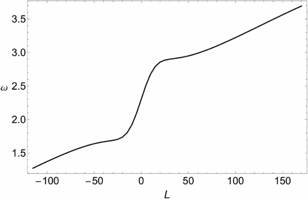
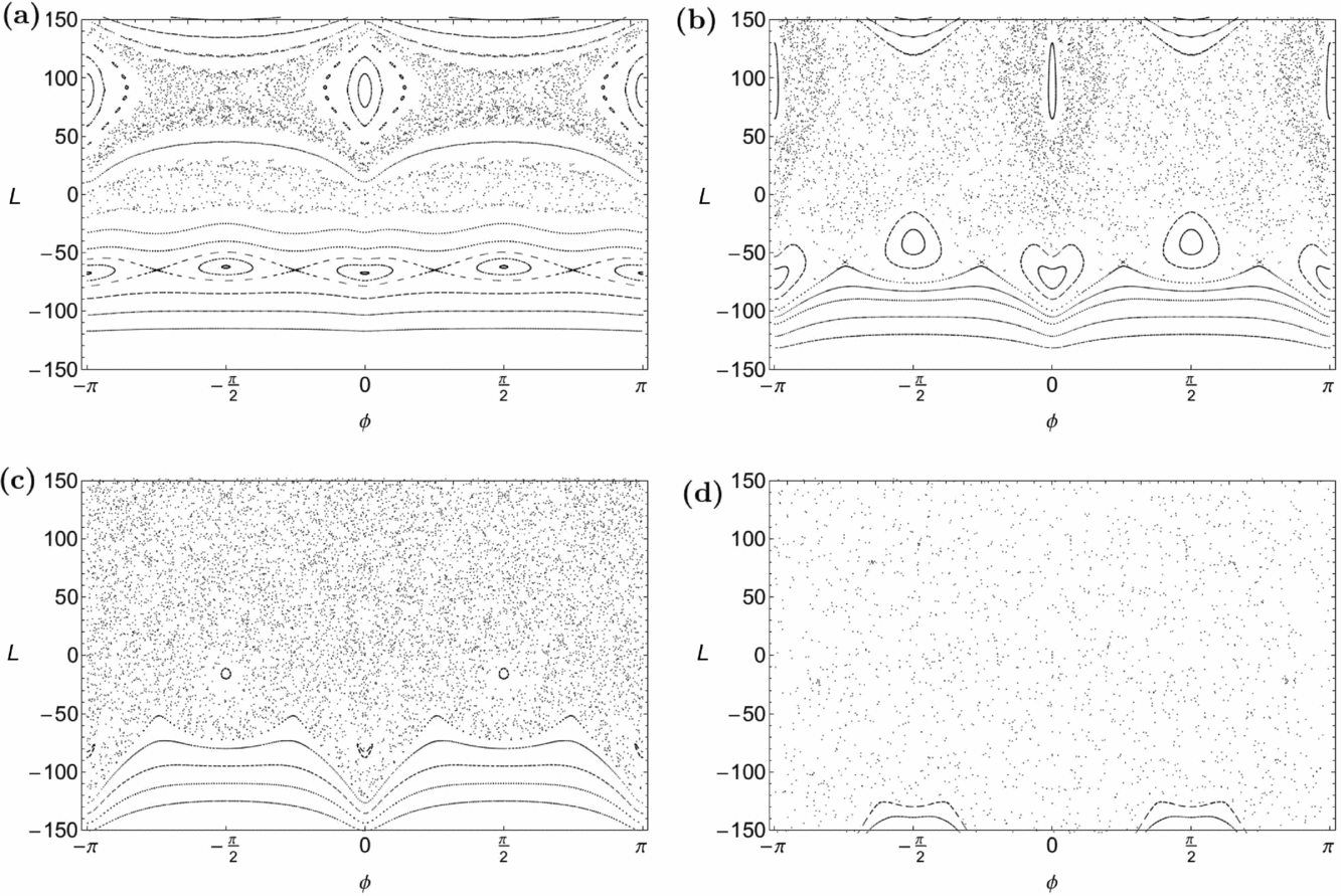
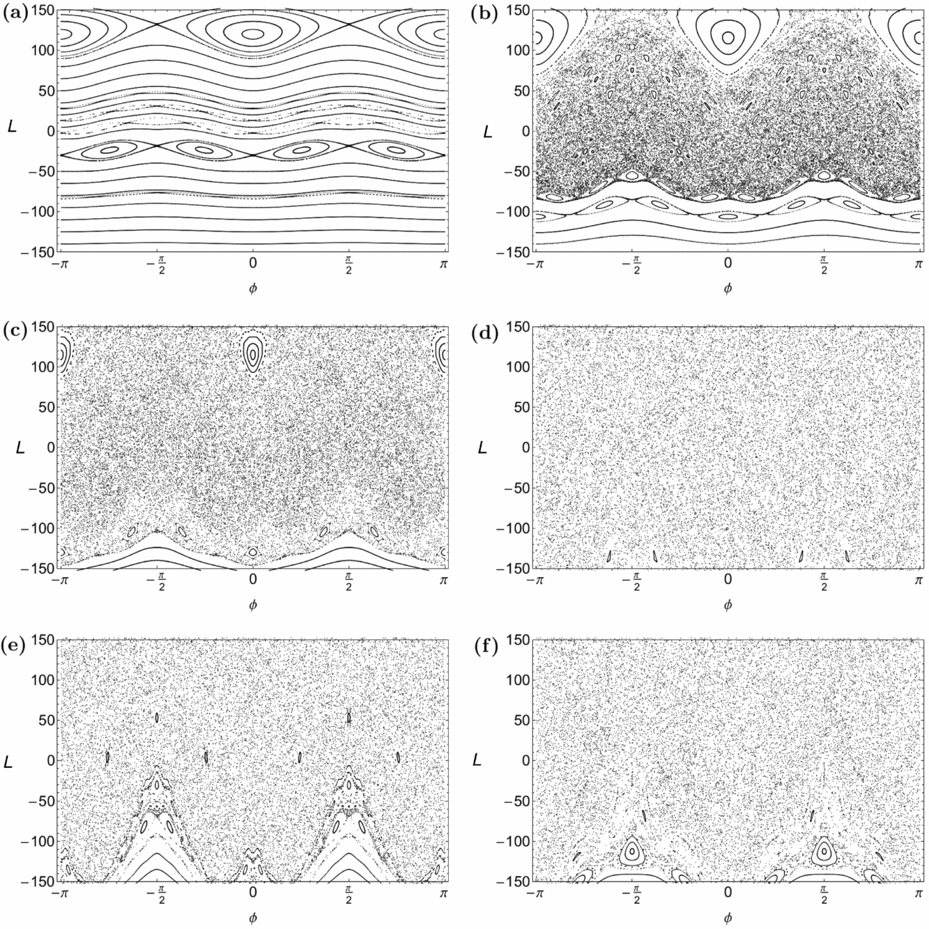
In the case M _b = 0, the bar has zero mass and therefore does not have any effect on the dynamics, i.e., the dynamics does not have any bar at all. Accordingly, the dynamics is rotationally symmetric, L is conserved, and P_r becomes a pure twist map. It is characterised by the rotation angle ω as function of L. In the position space of the rotating frame, the twist angle ω gives the angular advance of the orbit between two consecutive relative maxima of the radial coordinate. This twist curve is plotted in Figure 4. Note that for the integrable case M _b = 0, the values of a and c _b are irrelevant whereas these values matter for the details of the perturbation scenario away from the symmetric case. Under perturbations, i.e., here for M _b becoming different from zero, we expect k: n resonances to become important whenever the twist angle has the value 2πk/n for some small integer n. From the Figure 4, we expect a 1:4 resonance for L ≈ −70, a 1:3 resonance for L ≈ 0, and a 1:2 resonance for L ≈ 90. In Figure 5a–d, we show the perturbed map for four different non-zero values of M _b. For the small value M _b = 100 in part (a), we clearly see the large secondary 1:2 structure at a L interval around the expected value of approximately 90. We observe secondary KAM islands centred around the period 2 elliptic points at angle values ϕ = 0 and ϕ = π and a chaos strip organised by the hyperbolic period 2 points sitting at angle values ϕ = ±π/2. We also see clearly the 1:4 secondary structure around the L value − 70. Here, the fine chaos strips organised by the hyperbolic points still come very close to a separatrix curve. The expected 1:3 resonance structure has already decayed into a chaos strip even for the small value M _b = 100. As seen from Figure 4, the twist curve has a very large slope when it passes the value 2π/3 and therefore the corresponding resonance structure is extremely unstable and turns into a large scale chaos strip at very small perturbations. For values of M _b < 50, we see two different chains of very small secondary islands of period 3. Because of the discrete symmetry ϕ → ϕ + π in our system, the periodic points of odd period come in two different copies in general.

Figure 4.

The rotation angle ω as a function of the angular momentum L for M _b = 0.

Figure 5.

Examples of the perturbed map P_r for various values of the mass of the bar M _b when E = −900. (a-upper left): M _b = 100; (b-upper right): M _b = 500; (c-lower left): M _b = 1000; (d-lower right): M _b = 5000.

For the value M _b = 500 in part (b) of the figure, we still see the secondary KAM islands of the 1:2 resonance and also of the 1:4 resonance. The corresponding chaos strips have already merged to one global chaotic sea. For this value of M _b, we still find primary KAM curves for large positive and large negative values of L. As seen in part (c) of the figure, the secondary islands of the 1:2 resonance have disappeared for M _b = 1000 whereas the secondary 1:4 islands still exist on a very small scale. For this perturbation value also the primary KAM curves for large values of L have decayed. For the case of the very large value M _b = 5000 shown in part (d), there is little difference compared to the standard case. Only the secondary structures at large negative values of L have changed.

3.2. Dependence on the major axis of the bar

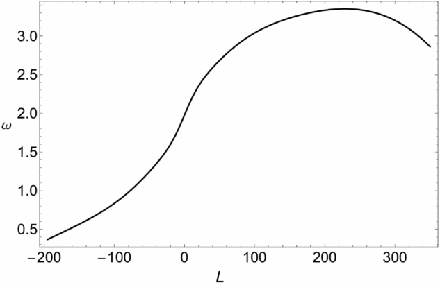
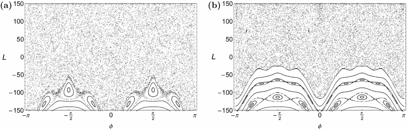
For a = 0, the bar is rotationally symmetric and therefore we have again a case where L is conserved and P_r is again a pure twist map which is characterised by its twist curve. The twist curve of this limiting case is presented in Figure 6. The most important resonances are a 1:2 resonance at L ≈ 120, a 2:5 resonance at L ≈ 40, a 3:8 resonance at L ≈ 20, a 1:3 resonance at L ≈ 0, a 1:4 resonance at L ≈ −25, and a 1:6 resonance at L ≈ −80. The perturbation of this twist map under a change of the parameter a is presented in Figure 7. For the small value a = 1 in part (a), we see the secondary structures expected from the twist curve of Figure 6. Remember that again the odd period structures of the 2:5 resonance and the 1:3 resonance come in two distinct copies. For this small value of the perturbation, all fine chaos strips are still very small and appear in the plots like separatrix curves.

Figure 6.

The rotation angle ω as a function of the angular momentum L for a = 0.

Figure 7.

Examples of the perturbed map P_r for various values of the major axis of the bar a when E = −900. (a): a = 1; (b): a = 2; (c): a = 3; (d): a = 5; (e) a = 7; (f): a = 9.

For a = 2 plotted in part (b), the L interval (−60, 80) is already dominated by a large scale chaotic sea in which many of the previously seen secondary structures are dissolved. For a = 3 shown in part (c), we see small remnants of the secondary 1:2 and 1:6 islands. Otherwise the only regular structures on a visible scale in the plot are the primary KAM curves for large negative values of L. There is another pair of islands at very large positive values of L ≈ 270 outside of the frame of the figure. For further increasing values of a, we approach the structure of the standard case without any further important changes in the large scale structure.

3.3. Dependence on the scale length of the bar

For c _b → ∞, we approach a rotationally symmetric case which is equivalent to the case M _b = 0. However, very large values of c _b do not describe realistic models of real galaxies. Therefore, we do not describe this limiting case in detail. In Figure 8, we just show the cases c _b = 0.1 and c _b = 2.5 to demonstrate that for realistic values of c _b there is little development of the dynamics at all under changes of c _b.

Figure 8.

Examples of the perturbed map P_r for various values of the scale length of the bar c _b when E = −900. (a-left): c _b = 0.1; (b-right): c _b = 2.5.

3.4. Dependence on the rotational velocity of the bar

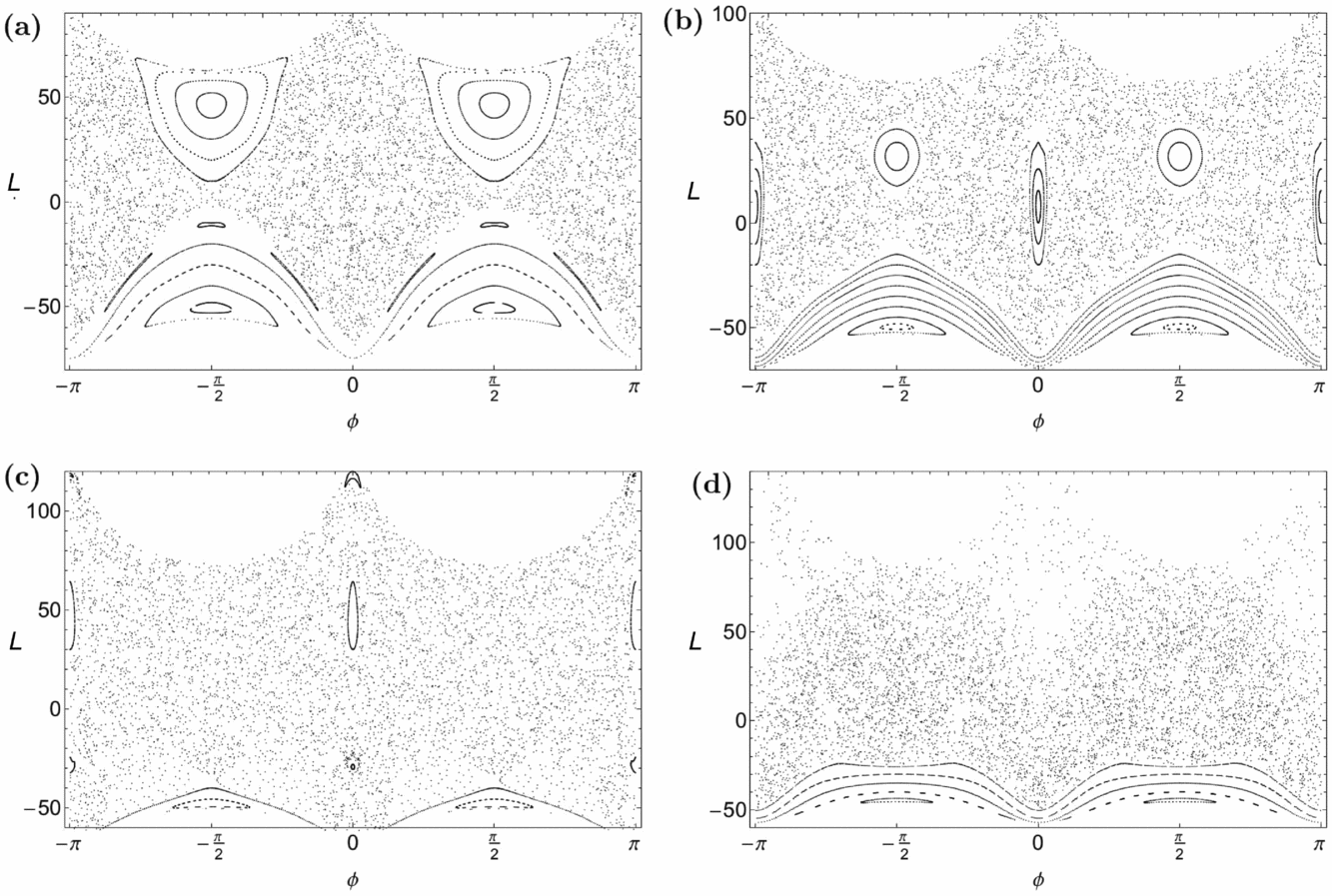
For increasing values of Ω_b, the dynamics becomes rather rapidly unstable because of the increasing centrifugal forces. Then, most orbits are scattering orbits which come from infinity and return to infinity. In this paper, our topic is not the chaotic scattering dynamics, we are only interested in bound motion. Therefore, we describe the dependence on Ω_b for a smaller value of the energy E where still a large part of the motion is bound also for values of Ω_b up to five. For the numerical examples, we choose the value E = −2400. Some examples of the corresponding map P_r are plotted in Figure 9. For Ω_b converging to zero, the map becomes upside down symmetric in L because for Ω_b = 0 the two orientations of angular motion become equivalent and correspondingly the sign of L becomes irrelevant. For Ω_b small and L not too close to zero the motion becomes stable for ϕ values around ± π/2. That is, motion around the origin and mainly perpendicular to the bar becomes dynamically stable.

Figure 9.

Examples of the perturbed map P_r for various values of the rotational speed of the bar Ω_b when E = −2400. (a-upper left): Ω_b = 1; (b-upper right): Ω_b = 2; (c-lower left): Ω_b = 3; (d-lower right): Ω_b = 5.

In part (a) of the figure for Ω_b = 1, we see two distinct island chains of period 2 with centres at ϕ = ±π/2, one at positive and one at large negative values of L. Increasing values of Ω_b break the symmetry between the two rotational orientations, i.e., between the two signs of L. The motion with positive values of L becomes unstable soon whereas the motion with large negative values of L remains stable up to very large values of Ω_b. Note that for intermediate values of Ω_b [see parts (b) and (c) of the figure] motion with small values of L and along the direction of the bar becomes stable. See the islands at ϕ = 0 and ϕ = π. The coming and going of these islands indicates that motion along the bar never becomes very unstable and that this type of motion can play the role of an important organisation centre of the dynamics also when it is slightly unstable.

In part (d) of the figure for Ω_b = 5, almost all the orbits of the large scale chaotic sea are in reality scattering orbits which go to infinity in the long run. For typical initial conditions in this chaotic sea, the orbit first increases its value of L to values above 500 and then the value of R becomes large monotonically, i.e., the orbit reaches the asymptotic region and does no longer produce any intersections with the surface of section of the Poincaré map. This transition to the asymptotic behaviour is not the topic of the present paper.

3.5. Dependence on the orbital energy

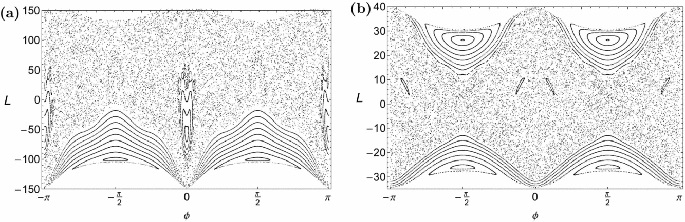
We have already seen a lot of maps for E = −900 and in the Ω_b series also some for E = −2400. Finally, let us see two more examples for different values of E. Figure 10(a) and (b) present the examples for E = −1650 and E = −3000, respectively, otherwise the plots are for the standard values of the bar parameters. In Figure 10, we see again the stable islands at ϕ = 0 and ϕ = π which also exist for some other parameter combinations. And for E = −3000, we see the large scale islands of period 2 at ϕ = ±π/2 and for both maximal positive and negative values of L.

Figure 10.

Examples of the perturbed map P_r for various values of the total orbital energy E. (a-left): E = −1650; (b-right): E = −3000.

The minimal possible value of the energy for the standard bar parameters is E = E _min = −4854. In the limit E → E _min, the motion converges to completely integrable harmonic motion even in 3-DOF. This is the last integrable limit case encountered in our study.

Certainly, the most persistent type of stable motion in S_z is the motion at the maximal negative values of L and in particular for angles in the neighbourhood of ϕ = ±π/2. We did not find any combination of reasonable realistic parameter values which makes this motion unstable. It is motion in negative orientation around the centre where the maximal values of R occur in the direction perpendicular to the bar. In comparison, motion mainly in direction of the bar is stable for limited parameter regions only. As Figure 7 shows, this last mentioned motion grows out of the 1:2 resonance of the integrable limit case a = 0 and it becomes unstable for a ≈ 4.7.

3.6. The x1 orbital family

As seen in Figure 7 for small values of a, the 1:2 resonance in the Poincaré map gives the largest secondary KAM islands. In this sense, the periodic orbit belonging to the central periodic point of these islands plays a prominent role in the dynamics. From the Poincaré maps, we observe that this orbit stays stable until a ≈ 4.7. And we expect that it still serves as an important organising centre of the dynamics also for larger values of a. Therefore, in this subsection, we study this periodic orbit in more detail.

In Figure 11a, we show the orbit in position space for the value a = 7. It is evident that it is an orbit moving mainly in the direction of the bar (x-axis) making at the same time smaller oscillations perpendicular to the bar directions(i.e., along the y-axis). Between these longitudinal and transverse oscillations in the bar potential, a 1:3 resonant coupling is evident. Orbits that are elongated parallel to the bar within co-rotation are known as x1 orbits and in this sense our main orbit is a 1:3 resonant x1 orbit. Along one complete revolution, this orbits runs through two maxima of R and therefore it appears as period 2 point in our Poincaré sections with the intersection condition that R is maximal.

Figure 11.

(a-left): An unstable x1 1:3 periodic orbit for a = 7 when E = −900; (b-right): The two left-right asymmetric x1 1:3 periodic orbits for a = 7 when E = −900. Note that one orbit is the mirror image of the other one.

In the next Figure 12a, we present graphically the stability type of this orbit, we plot the trace Tr of its monodromy matrix as function of a as the black curve. Remember that a periodic orbit is elliptic if − 2 < Tr < 2, it is normal parabolic if Tr = 2, normal hyperbolic if Tr > 2, inverse parabolic if Tr = −2, and inverse hyperbolic if Tr < −2. The eigenvalues λ of the monodromy matrix are obtained from the trace as

(14) $$\begin{equation} \lambda = Tr/2 \pm \sqrt{(Tr/2)^2 - det}. \end{equation}$$

And because the monodromy matrix is symplectic, we always have det = 1 for its determinant. Because of the importance of the values +2 and − 2 for the trace, two horizontal dashed lines (blue in the colour version) at these values are included in the figure.

Figure 12.

(a-left): Evolution of the trace of the monodromy matrix of the x1 1:3 family as a function of the major axis of the bar a when E = −900. The blue horizontal dashed lines at –2 and +2 delimit the range of the trace for which the periodic orbits are stable; (b-right): The characteristic curve of the x1 1:3 family.

As we have mentioned before, for a = 0, we have a pure twist map which is globally parabolic and therefore the curve in Figure 12a must start with the value Tr = 2 at a = 0. With increasing value of a, the eigenvalues run along the complex unit circle and when the phase of the eigenvalues reaches π then the trace reaches the value − 2. Because of discrete symmetry, the orbit does not become inverse hyperbolic at this point. It stays elliptic and the eigenvalue continues to run along the unit circle. For a ≈ 4.77, the eigenvalue reaches +1, the trace reaches +2, and here the orbit becomes normal hyperbolic in a pitchfork bifurcation. The trace curve of the original 1:3 x1 orbit passes through this bifurcation as smooth curve. At the moment of the change of stability, the original orbit splits off two descendants where each one breaks the left–right symmetry. But one of them is the mirror image of the other one. Figure 11b shows these two periodic orbits in position space for a = 7.

Figure 12b presents a bifurcation diagram of the pitchfork bifurcation. Here, the maximal value of the x coordinate of each one of the three orbits is plotted as function of a. The curve for a < 4.7 and the middle curve for a > 4.7 belong to the original symmetric 1:3 x1 orbit. The two outer branches for a > 4.7 belong to the two orbits split off in the pitchfork bifurcation. As long as the corresponding orbit is stable, the curve is green and when the orbit is unstable the curve in Figure 12b is red.

Also included in Figure 12a for a > 4.77 is the trace of the monodromy matrix of the asymmetric orbits split off in the pitchfork bifurcation. It is the lower curve in the figure. The split-off orbits are born with Tr = 2 and are stable in a small a interval. At a ≈ 5.04, the trace passes through the value − 2 and the orbits become inverse hyperbolic in a period doubling bifurcation. The orbits do not become very unstable for increasing a. After a first increase, the instability even returns to rather moderate values and around a = 10 the orbits are almost stable. Interestingly, also the instability of the original 1:3 x1 orbit saturates for these values of a. All these orbits become very unstable only for very large values of a outside of the range where the model makes physical sense. For extreme values of a, the split-off orbits change from 1:3 x1 type to 1:2 x1 type, i.e., then they make two transverse oscillations only for each longitudinal oscillation along the bar.

In total, we find the following situation for a ∈ (6, 10): There is a whole chaotic braid of 1:3 x1 orbits, the original left–right symmetric one, the two ones split of in the pitchfork bifurcations breaking the left–right symmetry, and the infinity created in the doubling cascades of the split-off orbits. At least some of them have rather moderate instability which implies that also the instability of the whole braid is moderate. And this in turn implies that this chaotic braid serves as an important organising centre for the whole dynamics.

4 NUMERICAL RESULTS FOR THE 3-DOF SYSTEM

A simple qualitative way for distinguishing between ordered and chaotic motion in a Hamiltonian system is by plotting the successive intersections of the orbits using a Poincaré surface of section (PSS). This method has been extensively applied to 2-DOF models, as in these systems the PSS is a two-dimensional plane (see Section 3). In 3-DOF systems, however, the PSS is four-dimensional and thus the behaviour of the orbits cannot be easily visualised.

One way to solve this problem is to choose a two- dimensional plane in the phase space, cover it with a sufficiently fine grid of points, use these points as initial conditions for orbits and check for each one of these orbits whether its motion is regular or chaotic, following the method used in Manos & Athanassoula (Reference Manos and Athansssoula2011); Zotos & Caranicolas (Reference Zotos and Caranicolas2013); Zotos (Reference Zotos2014). In this way, we are able to identify again regions of order and chaos, which may be visualised, because we choose as domains only planes of dimension-2. For most of our SALI plots, we use as domain the (x, z)-plane, choose for each orbit an initial point (x ₀, z ₀) in this plane, take three other initial conditions as y ₀ = p _x0 = p _z0 = 0 and obtain the last initial condition p _y0 from the value of the energy according to Equation (11), where we use the positive branch of the solution. Thus, we are able to construct again a two-dimensional plot depicting the (x, z)-plane. All the initial conditions of the 3D orbits lie inside the limiting curve defined by

(15) $$\begin{equation} f(x,z) = \Phi _{\text{eff}}(x,y = 0,z) = E. \end{equation}$$

In a few examples, we also show SALI plots on the (y, z)-plane as domain. They can be understood by exchanging the roles of x and y in the above mentioned construction.

For distinguishing between order and chaos in our models, we use the SALI method (Skokos Reference Skokos2001). We chose for each value of the free parameter of the effective potential, a dense uniform grid of 10⁵ initial conditions in the (x, z)-plane, regularly distributed in the area allowed by the value of the energy E. For each initial condition, we integrated the equations of motion (12) as well as the variational equations (13) with a double precision Bulirsch–Stoer algorithm (Press et al. Reference Press, Teukolsky, Vetterling and Flannery1992). In all cases, the value of the Jacobi integral [Equation (11)] was conserved better than one part in 10⁻¹¹, although for most orbits, it was better than one part in 10⁻¹².

All initial conditions of orbits are numerically integrated for 10³ time units which correspond to about 10¹¹ yr or in other words to about 10 Hubble times. This vast time of numerical integration is justified due to the presence of the sticky orbits. Therefore, if the integration time is too short, any chaos indicator will misclassify sticky orbits as regular ones. In our work, we decided to integrate all orbits for a time interval of 10³ time units in order to correctly classify sticky orbits with sticky periods of at least of 10 Hubble times. At this point, it should be clarified that sticky orbits with sticky periods larger than 10³ time units will be counted as regular ones, since such extremely high sticky periods are completely out of scope of this research.

Now, we use the SALI plots to observe the parameter dependence of the dynamics of the full 3-DOF system. To each Poincaré map from the previous section, we show the corresponding SALI plot. We begin with the SM in Figures 13 and 14, where Figure 13 is the SALI plot in the (x, z)-plane and Figure 14 is the SALI plot in the (y, z)-plane. The corresponding Poincaré plot has already been presented in Figure 3a.

Figure 13.

Regions of different values of SALI in a dense grid of initial conditions on the (x, z)-plane for the standard model.

Figure 14.

Regions of different values of SALI in a dense grid of initial conditions on the (y, z)-plane for the standard model.

Let us explain the connection between the Poincaré plot in the (ϕ, L)-plane and the SALI plot in the (x, z)-plane. The line z = 0 in the SALI plot belongs to the invariant subset S_z. The part for x positive corresponds to ϕ = 0 and the part for x negative corresponds to ϕ = π. For all points in the domain of the SALI plot, we have y = 0 and also p_x = 0, therefore automatically we have p_R = 0. Remember that the intersection condition of the Poincaré map is p_R = 0 with negative intersection orientation, i.e., p_R has to change from positive to negative, i.e., R has to run through a relative maximum.

We need to understand which points in the SALI plot corresponds to maxima of R and which ones to minima. When an orbit starts perpendicular to the SALI plane and with small value of the coordinate x then there is very little radial acceleration and the radial distance increases. In contrast, when the orbit starts with a large absolute value of x, then there is a strong acceleration in negative radial direction, the orbit starts with a large value of inward curvature and the initial value of R is a maximum. In this sense, approximately the outer half on both sides of the domain of the SALI plots corresponds to negative orientation with respect to the intersection condition p_R = 0 and the inner half on both sides corresponds to positive orientation of this intersection. It is also clear that points with positive x correspond to positive values of L and points with negative values of x correspond to negative values of L.

Accordingly, in total we have the following correspondence: Points on the outer half of the line segment z = 0, x > 0 in the SALI plot can be identified with points in the Poincaré plot along the line ϕ = 0 and positive values of L and points on the outer half of the line segment z = 0, x < 0 in the SALI plot can be identified with points in the Poincaré plot along the line ϕ = π and negative values of L. Analogous considerations hold for SALI plots in the (y, z)-plane where the corresponding values of ϕ are ± π/2. Here, we have only to remember that orbits start with positive values of p_x and therefore positive values of y in the SALI plot correspond to negative values of L and negative values of y in the SALI plot correspond to positive values of L. The outermost values of either x or y always correspond to L = 0.

Now, let us check this correspondence for the plots of the SM presented in Figures 3a–b, 13 and 14. In the Poincaré plot of Figure 3a, we see large scale regular structures for ϕ = ±π/2 and negative values of L only. Accordingly in Figure 13, we see no large scale regular structures at all for large absolute values of x and for z = 0 and in Figure 14, we see a small strip of regular behaviour along the line z = 0 for positive values of y.

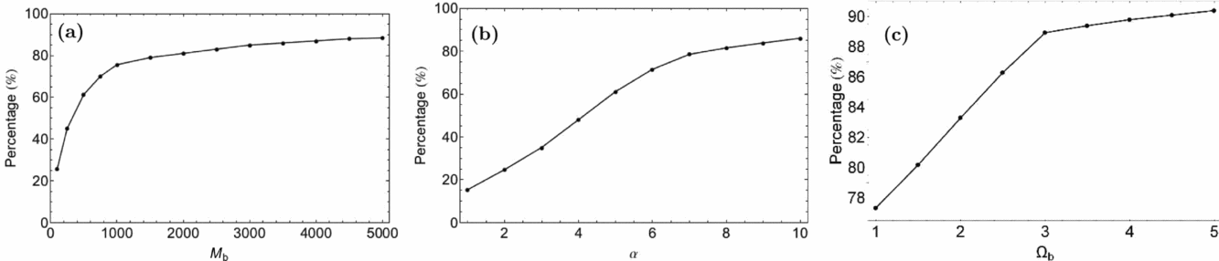
In the next figures, we show SALI plots in the (x, z)-plane for all cases for which we have given Poincaré plots in the invariant plane S_z in Section 3. Figure 15 shows the plots in dependence on M _b, Figure 16 contains the plots in dependence on a, Figure 17 shows the plots in dependence on c_b, Figure 18 gives the plots for various values of Ω_b, and finally Figure 19 shows the plots for two values of the total orbital energy E. In all cases, we can confirm the correspondence between SALI plots and Poincaré plots which we have explained above for the SM. In the Figures 20a–c, we show the relative fraction of chaotic orbits found in the SALI plots as function of M _b, a and Ω_b, respectively. Looking carefully at Figure 20a–c, it becomes evident that the percentage of the chaotic orbits in the (x, z)-plane increases in the following three cases: (i) when the bar becomes more massive, (ii) when the major semi-axis of the bar increases, and (iii) when the rotational velocity of the bar increases. In all three cases, for large enough values of the parameters (M _b > 3500, a > 9, Ω_b > 2.3) initial conditions of chaotic orbits dominate covering more than 85% of the (x, z)-plane.

Figure 15.

Regions of different values of SALI in a dense grid of initial conditions on the (x, z)-plane when E = −900. (a-upper left): M _b = 100; (b-upper right): M _b = 500; (c-lower left): M _b = 1000; (d-lower right): M _b = 5000.

Figure 16.

Regions of different values of SALI in a dense grid of initial conditions on the (x, z)-plane when E = −900. (a): a = 1; (b): a = 2; (c): a = 3; (d): a = 5; (e) a = 7; (f): a = 9.

Figure 17.

Regions of different values of SALI in a dense grid of initial conditions on the (x, z)-plane when E = −900. (a-left): c _b = 0.1; (b-right): c _b = 2.5.

Figure 18.

Regions of different values of SALI in a dense grid of initial conditions on the (x, z)-plane when E = −2400. (a-upper left): Ω_b = 1; (b-upper right): Ω_b = 2; (c-lower left): Ω_b = 3; (d-lower right): Ω_b = 5.

Figure 19.

Regions of different values of SALI in a dense grid of initial conditions on the (x, z)-plane. (a-left): E = −1650; (b-right): E = −3000.

Figure 20.

Evolution of the relative fraction of chaotic orbits found in the SALI plots on the (x, z)-planes as function of (a): M _b, (b): a and (c): Ω_b.

The great value of all these SALI plots lies in the following: By the comparison with the Poincaré plots, we obtain the information to which extent the regular structures found in the Poincaré plots are stable against perturbations in z direction. For the example of the SM, a comparison between Figures 3a and 14 shows that the regular structure at ϕ = ±π/2 and negative values of L in the Poincaré plot corresponds to a rather narrow stable strip around z = 0 and large values of y in the SALI plot of Figure 14. Accordingly, this stable structure is rather sensitive against out of plane perturbations and can be destroyed by moderate out of plane perturbations. In contrast, the stable structure along the line z = 0 in SALI plot of Figure 19b, the case for E = −3000, is very wide in z direction and therefore we conclude that the stable structure seen in the Poincaré plot of Figure 10b is rather stable against out of plane perturbations. Analogous considerations hold for all other parameter cases.

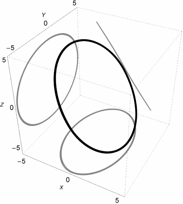
For most of the SALI plots, we see a large stable structure at small negative values of x and at large values of z. They correspond to tilted loop orbits which encircle the bar along a large loop, where the radial coordinate R is much larger than the width c_b of the bar, and tilted at an angle of approximately π/4 relative to the axis of the bar. This class of stable orbits seems to be the most persistent class of stable 3D orbits in our model. Figure 21 shows an example of such an orbit in position space with initial conditions: x ₀ = −3.3, y = 0, z ₀ = 4.45, p _x0 = 0, p _y0 > 0, p _z0 = 0. The existence of this class of orbits in triaxial rotating models of galaxies is known for a long time, see e.g., (Heisler, Merritt, & Schwarzchild Reference Heisler, Merritt and Schwarzchild1982).

Figure 21.

A characteristic example of an inclined 3D loop orbit along with its projections on the three primary planes.

5 THE SPIRAL STRUCTURE

It is well known that when stars escape from star clusters through the Lagrangian points, they form complicated structures known as tidal tails or tidal arms [e.g., (Capuzzo Dolcetta, Di Matteo, & Miocchi Reference Capuzzo Dolcetta, Di Matteo and Miocchi2005; Di Matteo, Capuzzo Dolcetta, & Miocchi Reference Di Matteo, Capuzzo Dolcetta and Miocchi2005; Just et al. Reference Just, Berczik, Petrov and Ernst2009; Küpper, Macleod, & Heggie Reference Küpper, Macleod and Heggie2008; Küpper et al. Reference Küpper, Kroupa, Baumgardt and Heggie2010)]. In the same vein, in the case of barred spiral galaxies, we observe the formation of spiral arms [e.g., (Ernst & Peters Reference Ernst and Peters2014; Grand, Kawata, & Cropper Reference Grand, Kawata and Cropper2012; Masset & Tagger Reference Masset and Tagger1997; Minchev & Quillen Reference Minchev and Quillen2006; Quillen et al. Reference Quillen, Dougherty, Bagley, Minchev and Comparetta2011; Roškar et al. Reference Roškar, Debattista, Quinn, Stinson and Wadsley2008; Sellwood & Kahn Reference Sellwood and Kahn1991)]. Usually, a star cluster rotates around its parent galaxy in a circular orbit. Thus, the tidal tails follow the curvature defined by the circular orbit and they are nearly straight for orbits moving in large galactocentric distances. The spiral arms of barred galaxies on the other hand, are formed by the non-axisymmetric perturbation of the bar. In particular, in barred spiral galaxies with prominent spiral-like shape, the two arms start from the two ends of the bar and then they wind up around the banana-shaped forbidden regions which enclose the Lagrangian points L ₄ and L ₅.

It would be very challenging to investigate if our simple gravitational model has the ability to realistically simulate the formation of spiral arms. We shall try to replicate the spiral structure of the SBb galaxy NGC 1300. According to Binney & Tremaine (Reference Binney and Tremaine2008) (plate 10) the semi-major axis of the bar is about 10 kpc. This means that we have to choose such values of the parameters so that the position of the Lagrangian points L ₁ and L ₂ to be at the two ends of the bar. For this purpose, we choose Ω_b = −3.5, while the values of all the other parameters remain as in SM.

In order to test this, we reconfigured our integration numerical routine so as to yield output of all orbits for a 3D grid of size $N_x \times N_y \times N_{\dot{x}} = 100 \times 100 \times 100$, when z ₀ = p _z0 = 0. This dense grid of initial conditions is centred at the origin of the physical (x, y) space and we allow for all orbits both signs of $\dot{y}$. Our purpose is to monitor the time-evolution of the path of the orbits and simulate the spiral arm formation. At t = 0, all orbits are regularly distributed within the Lagrangian radius inside the interior galactic region. In Figure 22, we present four time snapshots of the position of the 10⁶ stars in the physical (x, y)-plane. We observe that at t = 1 time units, which corresponds to 100 Myr the majority of stars are still inside the interior galactic region. However, a small portion of stars has already escaped passing through either L ₁ or L ₂. At t = 1.5 time units (150 Myr), we have the first indication of the formation of spiral arms, where with green and red colour we depict stars that escaped through Lagrangian points L ₁ and L ₂, respectively, while stars that remain inside the Lagrangian radius are shown in cyan. As time goes by, we see that the two symmetrical spiral arms grow in size and at t = 2 time units (200 Myr) the barred galaxy has obtained its complete spiral structure, while the interior galactic region is uniformly filled. In Figure 22a–d, the density of points along one star orbit is taken to be proportional to the velocity of the star according to Ernst & Peters (Reference Ernst and Peters2014). Being more specific, a point is plotted (showing the position of a star), if an integer counter variable which is increased by one at every integration step, exceeds the velocity of the star. Following this technique, we can simulate, in a way, a real N-body simulation of the spiral evolution of the barred galaxy, where the density of stars will be highest where the corresponding velocity is lowest. Therefore, we proved that for E = −1860 and Ω_b = −3.5 the scenario of evolution of spiral arms in our new barred galaxy model is indeed viable. Additional numerical simulations reveal that this is also true for other (lower or higher) values of energy. In fact, the particular energy level mainly controls how tight the spiral arms wind up around the forbidden regions of motion.

Figure 22.

The four parts of the figure show for four different values of the time the distribution of the position of 10⁶ stars in the physical (x, y)-plane initiated (t = 0) within the Lagrangian radius, for E = −1860 and Ω_b = −3.5. We see that as time evolves two symmetrical spiral arms are formed. The green arm contains stars that escaped through L ₁, while the red arm contains stars that escaped through L ₂. The bound stars inside the interior galactic region are shown in cyan, while the forbidden regions around L ₄ and L ₅ are filled with gray.