


1. Introduction
As a response to a globally changing climate, glaciers and ice caps worldwide have been retreating with increasing speed (e.g. Vaughan and others, Reference Vaughan, Stocker, Qin, Plattner, Tignor, Allen, Boschung, Nauels, Xia, Bex and Midgley2013; Huss and Hock, Reference Huss and Hock2018). Future climate change will likely have a significant impact on the dimensions of existing glaciers, which will affect the sea level and climate throughout the world. On regional scales, glacier retreat can affect hydropower production, freshwater availability, infrastructure and wildlife (e.g. Kaser and others, Reference Kaser, Grosshauser and Marzeion2010; Xu and others, Reference Xu, Yan, Kang and Ren2012). It is therefore important to investigate the effect of climate change on the cryosphere both on global and regional scales.
In order to asses the large-scale effects of a changing climate, state-of-the-art General Circulation Models (GCMs) are used internationally to make past and future projections. The Coupled Model Intercomparison Project (CMIP), for example, provides publicly available simulations from a large collection of models, with simulations spanning until at least 2100 (Taylor and others, Reference Taylor, Stouffer and Meehl2012).
However, due to the high computational cost of GCMs, they run with a coarse (100–200 km) resolution which does not resolve smaller glaciers. Dynamically downscaling climate projections from GCMs using Regional Climate Models (RCMs) is therefore a useful method to better resolve specific areas or surface processes. RCMs have been used and evaluated in several studies of the surface mass balance (SMB) of glaciers in, for example, Greenland (e.g. Box and Rinke, Reference Box and Rinke2003; Rae and others, Reference Rae2012; Fettweis and others, Reference Fettweis2016; Langen and others, Reference Langen, Fausto, Vandecrux, Mottram and Box2017), Antarctica (e.g. Lenaerts and Van Den Broeke, Reference Lenaerts and Van Den Broeke2012; Agosta and others, Reference Agosta, Fettweis and Datta2015) and Iceland (e.g. Schmidt and others, Reference Schmidt2017, Reference Schmidt2018).
Different RCMs and GCMs can project a highly variable climate response even when the same initializations and greenhouse gas concentration are used. It is therefore important to consider the output from several different models in order to sample a comprehensive range of possible climate trajectories. Therefore, for example, the Coordinated Regional Downscaling Experiment (CORDEX) (Giorgi and others, Reference Giorgi, Jones and Asrar2009) provides a large collection of publicly available historical and future simulations with different RCMs, driving GCMs (from CMIP phase 5), domains and initialization.
Most RCMs have a fixed topography, and therefore do not account for feedback caused by surface elevation changes nor for glacier retreat/advance. Coupling to an ice flow model is therefore needed in order to simulate a dynamically evolving glacier surface. Using RCMs to force ice flow models has been attempted in a number of studies (e.g. Aðalgeirsdóttir and others, Reference Aðalgeirsdóttir2011, Reference Aðalgeirsdóttir2014; Gong and others, Reference Gong, Cornford and Payne2014), which allows for a dynamically changing ice cap but does not include feedbacks on precipitation, temperature wind speed, etc., due to changes in surface elevation. Studies have shown that neglecting these feedbacks can lead to a significant underestimation in sea level projections (Edwards and others, Reference Edwards2014; Schäfer and others, Reference Schäfer, Möller, Zwinger and Moore2015). However, as a two-way coupling of climate models with ice flow models presents substantial computational challenges, fully coupled simulations are rarely performed. Some studies have attempted to solve this issue by adding an elevation-dependent correction to the simulated SMB in order to estimate the effect of the feedback (e.g. Edwards and others, Reference Edwards2014; Schäfer and others, Reference Schäfer, Möller, Zwinger and Moore2015).
Like most glaciers worldwide, Icelandic glaciers have been loosing mass since the late 1990s (Björnsson, Reference Björnsson2017). Vatnajökull ice cap, the largest ice cap in Iceland and the focus of this study, experienced slightly positive SMB in the 1980s, but SMB shifted towards negative after the mid-1990s following a sudden increase in sea-surface temperatures at the South-East coast (Björnsson and others, Reference Björnsson2013). The RCM HIRHAM5 has been used for studies of the climate of Vatnajökull by Schmidt and others (Reference Schmidt2017, Reference Schmidt2018). Only reanalysis-driven runs were used for these studies, and therefore only the reconstruction of the past climate was evaluated. Several other studies by, e.g. Aðalgeirsdóttir and others (Reference Aðalgeirsdóttir, Jóhannesson, Björnsson, Pálsson and Sigurðsson2006) and Aðalgeirsdóttir and others (Reference Aðalgeirsdóttir2011) have used RCM output for studies of the past and present climate of the ice cap, but these studies only use the precipitation and temperature fields from the RCMs to simulate the ablation using a positive degree day model.
In this study, the snow-pack scheme from the RCM HIRHAM5 (Langen and others, Reference Langen, Fausto, Vandecrux, Mottram and Box2017; Schmidt and others, Reference Schmidt2017) is used to simulate the climate of Vatnajökull until 2300, thus expanding on the work of Schmidt and others (Reference Schmidt2017). This is done by forcing the model with EC-EARTH simulations with a 5.5 km resolution and available CORDEX simulations with a 12 km resolution. The HIRHAM5-EC-EARTH simulations are also included within the CORDEX framework, but at a lower spatial resolution. Two greenhouse gas concentration scenarios are considered, Representative Concentration Pathways (RCP) 4.5 and 8.5. In the RCP 4.5 scenario (Reference ThomsonThomson and others), greenhouse gas concentration steadily increase until the radiative forcing stabilizes at 4.5 Wm−2 in 2100, where the average worldwide temperature has increased by ~ 2.4°C. The RCP 8.5 scenario (Riahi and others, Reference Riahi2011) is the RCP scenario with the highest projected greenhouse gas concentration, as the concentration increases significantly during the second half of the 21st century until the radiative forcing reaches 8.5 Wm−2 in 2100. The radiative forcing does not stabilize in this scenario, and it leads to an average worldwide temperature increase of ~ 4.7°C.
The RCM simulations are used to force the Parallel Ice Flow Model (PISM) (Bueler and Brown, Reference Bueler and Brown2009) in order to simulate the changes in glacier volume and area. PISM is one-way coupled to the RCMs, which means that any elevation feedback on the SMB is neglected. In order to estimate the sensitivity of the ice cap to elevation changes, precipitation and temperature lapse rates are added to some of the simulations.
This is the first study using PISM and distributed SMB fields from several RCMs to model the evolution of Vatnajökull. However, simulations of the whole ice cap or selected glacier outlets using flow models have been done in studies by, e.g. Björnsson and others (Reference Björnsson, Pálsson and Gudmundsson2001), Aðalgeirsdóttir (Reference Aðalgeirsdóttir2003), Aðalgeirsdóttir and others (Reference Aðalgeirsdóttir, Gudmundsson and Björnsson2005, Reference Aðalgeirsdóttir, Jóhannesson, Björnsson, Pálsson and Sigurðsson2006), Aðalgeirsdóttir and others (Reference Aðalgeirsdóttir2011), Flowers and others (Reference Flowers, Björnsson and Pálsson2003, Reference Flowers, Marshall, Björnsson and Clarke2005) and Marshall and others (Reference Marshall, Björnsson, Flowers and Clarke2005). The results of these studies will be discussed in the context of the simulations presented in this paper.
2. Study area and observations
2.1. Study area
Vatnajökull ice cap, currently ~ 7800 km2, is the largest temperate ice cap in Europe and is located close to the southeastern coast of Iceland (Fig. 1). At the highest areas of the glacier, there are only 10–20 days a year with melting, while at lower elevation the ablation season generally lasts 3–4 months (Björnsson and Pálsson, Reference Björnsson and Pálsson2008).
Vatnajökull ice cap. Shown are the locations of AWS stations (black triangles) and SMB/surface velocity sites (black dots) used in this study. The red lines show the ice divides.

Vatnajökull partly lies within the active volcanic zone, and covers several of Iceland's largest volcanoes where eruptions are frequent (e.g. Björnsson and Einarsson, Reference Björnsson and Einarsson1990; Gudmundsson and others, Reference Gudmundsson2012). Western Vatnajökull mainly lies on porous lava beds, while eastern Vatnajökull lies on impermeable unconsolidated till (e.g. Björnsson, Reference Björnsson1988). Tephra layers in the glacier ice dominate its spectral properties, and volcanic ash therefore has a large effect on the melt in the ablation zone (e.g. Larsen and others, Reference Larsen, Gonzalez-Pola, Fratantoni, Beszczynska-Möller and Hughes2016; Gascoin and others, Reference Gascoin2017; Schmidt and others, Reference Schmidt2017, Reference Schmidt2018). Frequent dust storms also occur over the ice cap, darkening the surface and increasing melt (e.g. Dragosics and others, Reference Dragosics2016). In addition to surface melting, geothermal activity below the glacier provides a small contribution to the total melt on average (Björnsson and Pálsson, Reference Björnsson and Pálsson2008).
All the major outlets of Vatnajökull are surge-type, and ~75% of the ice cap area can be affected by surges (Björnsson and others, Reference Björnsson, Pálsson, Sigurðsson and Flowers2003). Recorded surge histories suggest that some outlets surge at regular intervals (e.g. Brúarjökull surges every 80–100 years) while others surge at varying intervals (e.g. Breiðamerkurjökull surges every 6–38 years). In the 1990s, approximately 25% of the ice surplus in the accumulation area of Vatnajökull was transported to the ablation area by surges (Björnsson and others, Reference Björnsson, Pálsson, Sigurðsson and Flowers2003).
2.2. Available observations
Automatic Weather Stations (AWSs) have been operated on Vatnajökull since 1994, with 1–13 stations measuring on the ice cap during the summer months (e.g. Oerlemans and others, Reference Oerlemans1999; Björnsson and others, Reference Björnsson, Guðmundsson and Pálsson2006; Guðmundsson and others, Reference Guðmundsson, Björnsson, Pálsson and Haraldsson2006). Observations from five AWSs, three on Brúarjökull and two on Tungnaárjökull (Fig. 1), which have been operated at approximately the same locations since 2001, are used to evaluate the HIRHAM5-EC-EARTH simulations.
In situ SMB and surface velocity measurements have been carried out twice a year every glaciological year since 1991–92 (Björnsson and others, Reference Björnsson, Pálsson, Guðmundsson and Haraldsson1998), with an average of 60 measured locations every year (Fig. 1). The ablation has been observed using stake measurements, and the location of the stakes has been measured by GPS in order to estimate the average seasonal velocity. The uncertainty in the SMB measurements has been estimated to be ± 0.3 m water equivalent (w.e.) (Björnsson and others, Reference Björnsson, Pálsson and Guðmundsson1995, Reference Björnsson2013). Stake measurements are used to evaluate the SMB in HIRHAM5-EC-EARTH and the surface velocities in PISM.
The surface and bedrock topographies are needed as boundary conditions for PISM. For the surface topography, a surface elevation map of the ice cap from 2010 is used. The map is based on images from the Spot5 satellite (Berthier and Toutin, Reference Berthier and Toutin2008) from June and September 2010. The uncertainty on the acquisition day is ~1–2 m. However, due to differences between acquisition days in the surface elevation due to glacier melt, the uncertainty may be higher at ~5 m in some areas.
The bedrock topography maps are based on radio echo profiles from surveys since 1980 (Björnsson, Reference Björnsson1986, Reference Björnsson1988). Each pulse from the radio transmitter illuminates an approximate disc with a radius of ~100–200 m, thus the received echo is composed of energy from that area. An attempt to trace the energy to point sources at the bed is made using migration along the profile; a detailed description can be found in, e.g. Magnússon and others. The sounding lines were typically conducted 1 km apart and then interpolated to create a map using manual interpolation. The uncertainty along each sounding line is estimated to be ~±15 m (Björnsson, Reference Björnsson1988, Reference Björnsson2000), but due to uncertainty in the interpolation between the survey lines, the uncertainty of the bedrock topography map is estimated to be 20–50 m.
3. Model description
3.1. Regional climate models
HIRHAM5 is a hydrostatic RCM which combines the dynamical core of the HIRLAM7 numerical forecasting model (Eerola, Reference Eerola2006) and physics schemes from the ECHAM5 general circulation model (Roeckner and others, Reference Roeckner2003). The model configuration is described in detail in Christensen and others (Reference Christensen2006). In this study it is run over a domain containing Greenland and Iceland, with a horizontal resolution of 0.05° × 0.05° on a rotated-pole grid. This corresponds to ~5.5 km resolution. The atmospheric model has 31 vertical levels, from the surface to 10 hPa. The model time step is 90 s. HIRHAM5 model simulations have been successfully validated over Greenland (e.g. Box and Rinke, Reference Box and Rinke2003; Stendel and others, Reference Stendel, Christensen and Petersen2008; Lucas-Picher and others, Reference Lucas-Picher2012; Langen and others, Reference Langen2015, Reference Langen, Fausto, Vandecrux, Mottram and Box2017) and Iceland (Schmidt and others, Reference Schmidt2017) using AWS and ice core data.
However, when the model is forced by ERA-Interim reanalysis data (Dee and others, Reference Dee2011), which is a global atmospheric reanalysis by ECMWF spanning back to 1979, Schmidt and others (Reference Schmidt2017) found that there is an overestimation in the winter accumulation over parts of Vatnajökull which, e.g. affect the simulation of the albedo. Schmidt and others (Reference Schmidt2018) found that by using the well-evaluated snow pack scheme from HIRHAM5, but forcing it with incoming mass and energy fluxes from the numerical weather projection model (NWP) HARMONIE-AROME, a better agreement with SMB observations could be achieved.
HARMONIE-AROME is a non-hydrostatic, convection-permitting model (Bengtsson and others, Reference Bengtsson2017), which is based on the AROME-France model (e.g. Seity and others, Reference Seity2011), but now differs from the original model in various aspects (Bengtsson and others, Reference Bengtsson2017). Details on the model configuration are described in Bengtsson and others (Reference Bengtsson2017). In autumn 2015, the Icelandic Meteorological Office started a reanalysis project for Iceland (ICRA) using the HARMONIE-AROME model (details on the model setup can be found in Nawri and others (Reference Nawri, Pálmason, Petersen, Björnsson and Þorsteinsson2017)). ICRA currently spans from 1 September 1979, until 31 December 2017. It is run over a domain containing only Iceland at a horizontal resolution of 0.025° × 0.025°, corresponding to ~2.5 km. HARMONIE-AROME is forced by ERA-Interim reanalysis data at the lateral boundaries at 6 h intervals. Since HARMONIE-AROME is non-hydrostatic and calculates precipitation prognostically, it provides a better representation of the accumulation in areas with high orographic forcing than HIRHAM5 (Schmidt and others, Reference Schmidt2018).
Due to the better agreement between SMB observations and simulations when the snow pack scheme from HIRHAM5 is forced by HARMONIE-AROME meteorological forcing, the SMB from these runs is used for simulations in the reanalysis period (1980–present). In order to get a more accurate SMB, the precipitation scaling used by Schmidt and others (Reference Schmidt2018) is also used in this study. The method is described in detail in Schmidt and others (Reference Schmidt2018), and the details on the snow pack scheme are described in Langen and others (Reference Langen, Fausto, Vandecrux, Mottram and Box2017) and Schmidt and others (Reference Schmidt2017).
For future simulations, we rely on HIRHAM5 forced by EC-EARTH (Hazeleger and others, Reference Hazeleger2012) at the lateral boundaries as well as CORDEX simulations. EC-EARTH is based on the operational seasonal forecast system of the European Centre for Medium-Range Weather Forecasts (ECMWF). It has a 2°C cold bias over the Arctic (Koenigk and others, Reference Koenigk2013), which leads to an overestimation of the sea ice extent. However, it performs well when simulating dynamic variables, as comparison with other coupled models of similar complexity confirms (Hazeleger and others, Reference Hazeleger2012). In the CORDEX simulations, Iceland is represented both in the Europe and Arctic domains, but the highest resolution simulation (12 km) can be found in the Europe domain. Simulations which provided the output parameters needed for this study, have a resolution of 12 km and included an appropriate snow/ice mask over Vatnajökull were chosen. A list of the simulations is shown in Table 1.
CORDEX simulations used in this study

Two greenhouse gas concentration scenarios are considered, RCP4.5 and 8.5. Due to the high computational cost of the HIRHAM5-EC-EARTH simulations, they are only available in three 20-year time slices: a historical period from 1991 to 2010 and two future periods from 2031 to 2050 and 2081 to 2100. CORDEX simulations are available for the full period.
3.2. SMB modelling
In this study, the snow pack scheme from HIRHAM5, run offline from the atmospheric component, is used to simulate the SMB. The scheme has 25 subsurface layers, and includes a dynamic surface scheme that explicitly calculates the surface mass budget, accounts for the melting of snow and bare ice, and resolves the retention and refreezing of liquid water in the snow pack (Langen and others, Reference Langen2015, Reference Langen, Fausto, Vandecrux, Mottram and Box2017). This scheme only runs for designated glacier gridpoints, and it is run offline forced by 6 h surface energy (incoming shortwave (SW↓) and longwave (LW↓) radiation and turbulent fluxes) and mass fluxes (snow, rain, evaporation and sublimation) from a previous HIRHAM5 simulation. While a fully coupled, high-resolution HIRHAM5 run is computationally very expensive, this offline model offers a quicker alternative to test new model implementations.
This snow pack scheme has previously been evaluated for Vatnajökull by Schmidt and others (Reference Schmidt2017). The authors used an updated snow albedo scheme, which was tuned to better fit with observations from AWSs operated on Vatnajökull. In addition, the albedo of the ice that emerges as the snow melts away in the ablation zone, was improved by using a background map based on MODIS observations (Gascoin and others, Reference Gascoin2017; Schmidt and others, Reference Schmidt2017). This version of the model is used in this study.
The offline model can be forced by incoming energy and mass components from another climate model, although then additional missing feedbacks have to be taken into considerations. Schmidt and others (Reference Schmidt2018) used the model forced with energy and mass fluxes from the NWP HARMONIE-AROME, and achieved improved simulations of the SMB compared to using HIRHAM5 forcing. A similar approach will be used in this study, as the CORDEX simulations will all be used to force the snow pack scheme. This is done in order to get the most similar conditions for the climate runs, and the differences in SMB are not due to, e.g. different complexities of the albedo parameterization. The way the output from RCMs can be used to force the HIRHAM5 snow pack scheme is described in detail in Schmidt and others (Reference Schmidt2018).
The calculated monthly SMB fields are used to force the ice flow model PISM (Bueler and Brown, Reference Bueler and Brown2009), in order to get an estimate of the future volume and area change of the ice cap. Since this is a one-way coupling, the elevation-SMB feedback is not taken into account. To assess the importance of this feedback, a set of model runs where a lapse-rate correction is added to the precipitation and temperature are also conducted. A lapse rate of δP/δh s = 0.00176 a−1 is used following Flowers and others (Reference Flowers, Marshall, Björnsson and Clarke2005), where P is the precipitation and h s is the surface elevation in metres, and a temperature lapse rate of δT/δh s = 0.006 K/m following Guðmundsson and others (Reference Guðmundsson, Björnsson, Pálsson and Haraldsson2006) is used to correct the incoming longwave radiation and the sensible heat flux, as these fluxes can both be parameterized as a function of the air temperature. The effect on the latent heat flux is assumed negligible. If the temperature at 2 m above the surface becomes warmer than 2°C, snowfall is transformed into rain. A schematic of how the models are coupled for these runs is shown in Figure 2. Feedbacks due to changes in humidity and wind speed have been assumed negligible for these runs.
The setup of the model coupling. The precipitation and temperature lapse rate corrections are only added for the elevation feedback experiments.

3.3. PISM
PISM (Bueler and Brown, Reference Bueler and Brown2009) is an open-source, 3-D, thermo-mechanically coupled ice-sheet model which has been applied in various studies of the Antarctic and Greenland ice sheets (e.g. Winkelmann and others, Reference Winkelmann2011; Aschwanden and others, Reference Aschwanden, Aðalgeirsdóttir and Khroulev2013, Reference Aschwanden, Fahnestock and Truffer2016; Aðalgeirsdóttir and others, Reference Aðalgeirsdóttir2014). PISM numerically solves the shallow ice and shallow shelf approximations (SIA and SSA) in parallel. The SIA is solved with a non-sliding base, and the SSA can be used to estimate basal sliding (Bueler and Brown, Reference Bueler and Brown2009). In this study, both the SIA and the combined SIA+SSA schemes are investigated for Vatnajökull using PISM version 1.0.
3.3.1. Sliding and deformation
Basal sliding in PISM can be estimated using a fully plastic or pseudo-plastic law. In the case of a pseudo-plastic power law, it relates bed-parallel shear stress, $\vec {\tau _{\rm b}}$ , to the basal velocity $\vec {u}_{\rm b}$
 (Bueler and Brown, Reference Bueler and Brown2009)

where τc is the yield stress, which represents the strength of the glacier till, $\vec {u}_{{\rm threshold}}$ is a threshold speed, and q is the pseudo-plastic exponent. Setting q = 0 gives the fully plastic case. Sliding is likely to occur if the driving stress is larger than the yield stress. The yield stress can either be considered constant or calculated dynamically by relating the till material properties, i.e. the till friction angle ϕ, and the effective pressure on the till, N till, using the Mohr–Coulomb criterion:

where c 0 is called the till cohesion and is generally set to zero. The effective pressure on the till is determined by The PISM authors (2018)

where P o is the ice overburden pressure, determined entirely by the ice thickness, density and the gravitational acceleration, and W till is the effective thickness of water in the till computed in the model. The remaining variables are constants which describe the till mechanics: N 0 = 1000 Pa is the reference effective pressure of the till, δ is the effective fraction overburden, e 0 = 0.69 is the reference void ratio, C c = 0.12 is the compressibility coefficient and $W_{{\rm till}}^{\max }=2$ m is the maximum water thickness allowed in the till (Tulaczyk and others, Reference Tulaczyk, Kamb and Engelhardt2000; Bueler and van Pelt, Reference Bueler and van Pelt2015).
The till friction angle ϕ is a measure of the ability of the till to withstand a shear stress and can either be set as a constant or determined as a linear function of the bedrock elevation. The elevation dependence is expressed as follows

where b min, b max, ϕ min and ϕ max are chosen constraints on the bed elevation and till friction angle, respectively.
While till deformation plays a major role in the ice flow of parts of, e.g. Greenland, till deformation may not be the main reason for basal sliding beneath Vatnajökull. Therefore, we do not claim that the sliding model in PISM describes the physics of basal sliding beneath Vatnajökull, but by tuning the parameters of the till model, basal sliding which is in accord with the observed velocities may be simulated.
PISM is highly customizable, for example, including a hierarchy of flow laws with different complexities. In this study, tests are conducted using the isothermal Glen's flow law, where the ice softness A is constant but can be determined manually.
Previous studies have determined what the optimal parameters are for the ice sheets on Greenland (e.g. Aschwanden and others, Reference Aschwanden, Aðalgeirsdóttir and Khroulev2013) and Antarctica (e.g. Winkelmann and others, Reference Winkelmann2011). A similar determination of parameters is conducted for Vatnajökull before the model is used for coupled simulations.
3.3.2. PISM boundary conditions
To simulate the ice flow with PISM, the model needs the following boundary conditions; the bedrock elevation, an initial ice thickness estimate, a geothermal heat flux map, the monthly mean SMB and the monthly mean ice surface temperatures. The bed elevation and initial ice thickness maps have a resolution of 0.5 × 0.5 km and are based on observations.
When using a SMB field to force PISM, the ice temperature, i.e. the temperature below snow and firn processes, is required as model input. Icelandic glaciers are temperate (Björnsson and Pálsson, Reference Björnsson and Pálsson2008), and while a winter cold wave is observed in the glacier snow, it generally does not reach deep into the underlying ice. Using HARMONIE-HIRHAM5 climate forcing, a 1000-year equilibrium run with an active enthalphy model produce that 80% of the ice cap is temperate. For example, the ablation zones of Brújökull and Dyngjujökull show cold bases below pressure melting. Based on field observations, this is not realistic. We therefore decided to rather prescribe a constant ice temperature of 0°C for all of Vatnajökull, ensuring temperate ice everywhere
Several simulated SMB fields are used in this study, as described above. If the flow model is run at the resolution of the RCMs, i.e. with a grid size ${\ges }2.5\, {\rm km}$ , high velocity areas occur due to the large topographic gradients between grid points at this resolution. The SMB fields are therefore interpolated onto the 500 m grid of the bedrock and surface maps using bi-linear interpolation, which results in a more accurate representation of the surface velocities.
An important source of meltwater beneath Vatnajökull is due to geothermal heat flux. A NW-SE heat-flux gradient surrounds Vatnajökull, with maximum heat fluxes of 0.25 Wm−2 above the active rift zone (Flóvenz and Saemundsson, Reference Flóvenz and Saemundsson1993). Some central volcanoes have much higher localized values of up to 50 Wm−2. The basal water computed in PISM is important, e.g. for determining the saturation of the till. In the absence of a map of geothermal heat fluxes, the method used by Flowers and others (Reference Flowers, Björnsson and Pálsson2003) is used to estimate the background fluxes. The eastern sector of Vatnajökull is assigned a value of 0.18 Wm−2, while the western sector is assigned no heat flux since the subsurface hydrothermal circulation is assumed to be sufficiently strong to prevent heat from reaching the ice. Active geothermal areas at Grímsvötn and the Skaftá cauldrons are assigned a heat flux of 50 Wm−2 following the suggestion of Björnsson (Reference Björnsson1988).
4. Experimental setup
Before projections of the future evolution of Vatnajökull can be conducted, the coupled RCM-ice flow model needs to be initialized to represent the present state of the glacier, as the starting model state strongly influences the short-term trajectory of projections (e.g. Aðalgeirsdóttir and others, Reference Aðalgeirsdóttir2014).
In this study, a constant climate spin-up is conducted using a constant ice temperature. The simulated climate from 1980 to 1999 is used for a 1000-year spin-up, as Vatnajökull was approximately in balance during this period. After the spin-up, the model is forced until 2010 for comparisons with the observed geometry of that year.
It is important to note that Vatnajökull is most likely not in a steady state; previous studies have shown that the current shape can be best represented by an ice cap that is not in equilibrium with the current climate (e.g. Aðalgeirsdóttir and others, Reference Aðalgeirsdóttir, Gudmundsson and Björnsson2005; Marshall and others, Reference Marshall, Björnsson, Flowers and Clarke2005). One of the explanations for a non-equilibrium ice cap is that most of the outlets of Vatnajökull are surge-type. Surges have a major effect on the shape and SMB of Icelandic glaciers, with ~25% of the surplus in the accumulation area of Vatnajökull being transported down-glacier by surges in the 1990s (Björnsson and others, Reference Björnsson, Pálsson, Sigurðsson and Flowers2003). Performing a spin-up without surges is therefore expected to produce an ice cap with a too large volume and too small area. Since PISM does not include physics to initiate surges, it is not possible to have dynamically occurring surges in the model.
The final spin-up state is then used for both equilibrium and continuous simulations. For the equilibrium simulations, the climate from the EC-Earth time slices are repeated until a steady state is reached in order to determine the response time of Vatnajökull to different changes in climate.
The continuous runs use the climate forcing from HARMONIE-AROME, EC-EARTH and CORDEX to simulate the climate until 2100. After 2100, the climate from 2081 to 2100 is assumed to continue until 2300. While CORDEX simulations are continuous until 2100, the high resolution of the 5.5 km EC-EARTH runs mean that only 20-year time slices are available. In between the time slices, the SMB is simulated by adding a linear trend between the time slices with the variability from the previous period added to the trend.
Since the SMB simulations from CORDEX and HIRHAM5 are forced by freely running GCMs, significant biases may be present. As an example, the temperature of HIRHAM5 forced by EC-EARTH is compared to observations from five AWSs in Figure 3. The climate of EC-EARTH has (as any freely running GCM) a variability that is out of phase with reality, and comparison with observations is therefore best done using a statistical method.
Quantile–quantile plots of the monthly mean temperatures from five AWSs compared to (a) EC-EARTH forced simulations and (b) ERA-Interim forced simulations. Red line shows the straight line the quantiles follow and the black line shows a one-to-one line.

Figure 3 therefore shows quantile–quantile plots of the modelled and observed monthly mean temperatures. Both the EC-EARTH and ERA-Interim forced simulations are compared to the temperatures measured at five AWSs from 2001 to 2010 (locations marked in Fig. 1). The figures show that statistically the EC-EARTH and ERA-Interim forced simulations are from a similar distribution as the observations, as all the results lie on an approximately straight line (shown in red) except at low temperatures. However, there is a clear temperature bias in the EC-EARTH runs. EC-EARTH has a 1.9°C cold bias over Vatnajökull, which is consistent with the general 2°C cold bias found over the Arctic in EC-EARTH (Koenigk and others, Reference Koenigk2013). In comparison, ERA-Interim forced HIRHAM5 simulations have a cold bias of 0.4°C over Vatnajökull (Schmidt and others, Reference Schmidt2017).
Since a temperature bias was found for the EC-EARTH simulations, the SMB is generally overestimated in these runs. If the SMB fields were used directly to force the ice flow model, large biases would be introduced into the volume calculations. Therefore, instead of using the absolute values computed by the offline model, the flow model can be forced with SMB anomaly fields. These are computed by subtracting the projections for each year from the mean of the historical period. The anomaly is then added to the average HARMONIE-HIRHAM5 simulated SMB from 1991 to 2010. This is done by interpolating the anomaly map onto the HIRHAM5-HARMONIE coordinates. Therefore, anomaly corrected SMB fields are used to force the ice flow model. The specific SMB of the corrected fields are shown in Figure 4. Although the anomaly corrected simulations still do not capture the yearly variability, the average mass balance for the period 1991–2010 is similar.
The simulated, anomaly corrected SMB by HIRHAM5-EC-EARTH using the RCP 4.5 and RCP 8.5 scenarios. Black lines with coloured dots show the observations.

EC-EARTH simulations are not the only ones with large biases, and the average CORDEX SMB values differ from the observations by − 1 to 2 m a−1. We therefore also apply the above anomaly approach to the CORDEX projections.
Although this method does correct some of the biases from the RCMs, it does not change the ratio of rainfall versus snowfall. In climate models where the temperature is too cold, like e.g. EC-EARTH, this ratio will most likely be underestimated. In addition, since melt does not increase linearly with temperature, the melt increase is likely also underestimated. Thus the anomalies computed over a too cold climate are likely underestimated compared to anomalies computed with a more accurate climate.
5. Results
5.1. Determining optimal flow law and sliding parameters in PISM
A series of simulations are performed to assess the optimal parameters for simulating the flow of Vatnajökull. First, a 1000-year fixed geometry spin-up is conducted until the glacier ice and till are in a steady state. Then, a 1-year simulation with changing geometry is conducted to slightly smooth the surface but still retain the present day geometry. This method has previously been used by, e.g. Aðalgeirsdóttir and others (Reference Aðalgeirsdóttir, Gudmundsson and Björnsson2005). The 1-year ice surface velocities are then compared to available observations.
First, we determine if the observed ice velocities can be simulated without sliding (i.e. SIA only). We find that while the measured velocities can be simulated without sliding, different viscosities are needed for each outlet. A better model choice is to choose a softness that simulates the lowest measured velocities, which can be assumed to be due to deformation only, and add sliding to the simulations. The closest fit to the minimum observed velocity (assumed to be the deformation velocity) is achieved using isothermal Glen's flow law with A = 2.4 · 10−24 s−1Pa−3 (see Fig. 5), which is the value suggested for temperate ice by Cuffey and Paterson (Reference Cuffey and Paterson2010).
Comparison of flow velocities after 1 year with measured velocities at the SMB stakes (Fig. 1) for (a) western Brúarjökull, (b) eastern Brúarjökull, (c) Köldukvíslarjökull, (d) Síðujökull, (e) Tungnaárjökull, (f) Dyngjujökull, (g) Breiðamerkurjökull and (h) Eyjabakkajökull. The horizontal axis is the distance from the ice divide. The red dots show the simulated velocities using only SIA with A = 2.4 · 10−24 s−1Pa−3, assumed to be equivalent to the deformation velocity, and the blue dots show SSA+SIA velocities when the options in Table 2 are used. Solid black line shows the average over the observation period, while stippled black lines show the maximum and minimum observation.

Model choices changed from the PISM default settings
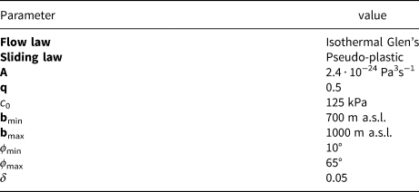
The estimation of sliding, when using SSA, shows the best fits with observations when a pseudo-plastic flow law with a till friction angle ϕ that is linearly dependent on the bedrock elevation is used. However, a large velocity mismatch arises for points near the outlet terminus. The only way to counter this effect and still allow sliding in other areas is to add a large till cohesion c 0 of ~125 kPa. The changes from the default PISM settings are summarized in Table 2. These settings were found by slowly varying each of the parameters and comparing the resulting velocities to observations. A full list of all PISM parameters can be found in The PISM authors (2018).
The simulated velocities with the PISM setup described in Table 2 are shown along eight flow lines in Figure 5. The modelled velocities of Brúarjökull and Köldukvíslarjökull have the best fit with the average observations. Breiðamerkurjökull has the largest deviation, but the simulated velocities are still mostly within the range of the observations. Eyjabakkajökull is the only outlet which significantly deviates from the observations, which suggest that generally very little sliding occurs along this outlet. Brúarjökull, Síðujökull, Breiðamerkurjökull and part of Dyngjujökull are most affected by sliding.
5.2. Model spin-up using 1980–99 climate
The results of the constant climate spin-up are shown in Figures 6a, b. As expected, the equilibrium state has a smaller area (by 2.5%) and a larger volume (by 3.5%) compared to the present day reference geometry, which is partly due to the lack of surges in the model. Dyngjujökull has the largest deviation in thickness, which could be due to the short surge cycle (~20 years) of this outlet. The flow of the glacier is not large enough to transport the accumulated mass down to the ablation area, and thus the glacier thickens and prepares for a surge. Brúarjökull, on the other hand, has a long surge cycle of 80 years. The simulated outlet is still thicker and shorter than the current geometry, but the thickness is generally overestimated by less than 50 m, whereas Dyngjujökull is overestimated by between 50 and 150 m. The thickness of the south-facing outlets is underestimated in the ablation zone and overestimated in the accumulation zone, which could partly be attributed to the fact that there are no surges in the model to bring excess mass from the accumulation zone down to the ablation zone.
(a) The surface elevation and the outline of the reference extent (white) and the spin-up extent (purple). (b) The elevation difference between the reference ice surface and the model after the constant climate spin-up. (c)–(h) The spin-up profiles compared to observed 2010 profiles from six outlets. Profiles are shown with black lines in (a).

As previously mentioned, the present day ice cap is most likely not in equilibrium with the current climate and thus an equilibrium ice cap will not capture the present day geometry even if surge dynamics are included. A non-equilibrium present day geometry, e.g. explains the thin ice at the terminus of several outlets which disappear during the constant climate spin-up. Errors in the reanalysis forcing and the bedrock topography also affect the spin-up geometry.
Figures 6c–h show the profiles of six outlets along a flowline both for the observed 2010 geometry and for the simulated geometry. As previously mentioned, Brúarjökull and Dyngjujökull are the outlets with the largest differences between the spin-up geometry and the observed geometry. After the spin-up, Brúarjökull is ~7.5 km shorter in the simulation. Therefore, it is the outlet whose extent is the furthest from the observed. The simulated Dyngjujökull is 2 km shorter, while the simulated Skeiðarárjökull and Tungnaárjökull are ~3 km shorter. Hoffellsjökull and Breiðamerkurjökull have the same extent in the simulations as observed.
Due to these changes in area and thickness, the simulated velocities for this geometry do not fit as well with the observations as in the 1-year geometry run. The root mean square error (rmse) of the difference between observed and simulated surface velocities at the end of the spin-up are given in Table 3. A main reason for the bigger errors is that the edges of the ice cap have become steeper compared to the 1-year run, hence the velocities become higher near the outlet terminus. Especially Dyngjujökull, which has the highest deviation in thickness in the steady-state simulations, reaches velocities much higher than those simulated with the current geometry (see Table 3).
The mean root-mean-square error between average observed and simulated surface velocities for all measurement sites.

Note: The 1-year velocities are modelled using the observed 2010 outlet geometry, while CC spin-up velocities are taken at the end of a constant climate spin-up
5.3. Reanalysis simulations from 1980 to 2016
The simulated changes in SMB, volume and area of Vatnajökull during the period 1980–2016 are shown in Figure 7. The measured change in volume from the 1991–92 glaciological year until 2014–15 is ~3% (Pálsson and others, Reference Pálsson, Gunnarsson, Jónsson, Steinþórsson and Pálsson2015). In the model simulations, the volume loss is approximately half of the observed: 1.7% since 1991–92. This is due to an overestimation of the net balance from 1995 to 2000 (see Fig. 7a), as well as the effect of volcanic eruptions on the albedo and thus the surface ablation. The glacier surface was affected by tephra from eruptions occurring in 1996, 1998, 2004, 2010 and 2011. The facts that parts of the ablation zone disappeared during spin-up, and that surges occurred in 1991, 1994 and 2000 in western and north-western outlets, which transported additional mass down to the ablation zone, also contribute to the difference in volume loss.
(a) HARMONIE-HIRHAM5 reconstructed summer (red), winter (blue) and net (green) SMB compared with observations (black); (b) volume and (c) area in simulation from 1980 to 2015.

The simulated change in area is also shown in Figure 7c. Only very small changes are simulated during the reference period: 1.2% from 1991–92 to 2014–15. This small change is because the spin-up state is in balance with the 1980–1999 climate, and that the thinnest parts of the ablation zone disappeared during the model spin-up.
5.4. Equilibrium decline
5.4.1. Step-wise ice cap decline
To estimate the response of the ice cap to a sudden climate change, the flow model is first forced with the climate forcing for each of the HARMONIE-EC-EARTH time slices. Starting from the spin-up state, the model is run for 2000 years recycling the anomaly of the forcing from 2031 to 2050 and 2081 to 2100 for the RCP 4.5 scenario, and 2081 to 2100 for the RCP 8.5 scenario. This corresponds to a sudden temperature change of 1.5, 3.0 and 4.7°C over Iceland. The resulting changes in area and volume are shown in Figure 8a–c.
Changes in ice cap volume and area with step-wise climate forcing. Figures (a)–(c) do not take elevation feedback into account, while Figures (d)–(e) use a lapse rate correction. Figures (a) and (d) show the volume change relative to the reference ice cap, (b) and (e) show the area change relative to the reference, and (c) and (f) show the steady-state area at the end of the simulations.

For the 2031–2050 RCP 4.5 scenario (1.5°C warming) the ice cap stabilizes at a volume and area that are 30 and 16% smaller than the starting value, respectively. For the 2081–2100 RCP 4.5 scenario (3.0°C warming) the ice cap takes longer to reach a steady state than the other two scenarios, but the volume and area eventually stabilize at a 66% smaller volume and a 40% smaller area. For the last scenario, 2081–2100 RCP 8.5 with 4.7°C warming, only the highest points of the ice cap (e.g. Öræfajökull and Bárðarbunga) stay glacierized. Here, 97% of the volume and 92% of the area have disappeared. The current glaciation limit for southern Iceland is 1100 m (Björnsson and Pálsson, Reference Björnsson and Pálsson2008), so if the ice cap disappears, it may not grow back during the current climatic conditions. However, because there is no elevation feedback in these runs, the ice cap will rebuild until it reaches the spin-up state if the climate is returned to that of 1980–99 in these simulations.
When adding a precipitation and temperature lapse rate to the forcing, to estimate the effect of elevation feedback on the SMB, the response of the ice cap is slightly faster (Figs 8d–f). After 200 years, the lapse rate runs have volumes and areas that are 5–11 and 3–18% smaller than the runs without a lapse rate correction, respectively. Initially, the RCP 8.5 run has the largest sensitivity to the lapse rate correction, but since the ice cap almost disappears even in the run without the lapse rate correction, there is not a large difference between the steady-state configurations. Once the ice cap reaches a steady state, the lapse rate simulation projects a volume and area that are only 2 and 4% smaller than the simulations without the correction. The two more moderate warming scenarios (1.5 and 3.0°C warming) are more sensitive to the elevation-dependent feedback. After ~300 years, the volume and area drop below those found without the lapse rate correction and keep decreasing for the rest of the run. At the end of the 2000-year run, the simulation with a 1.5°C temperature increase has a volume and area that are 46% and 36% smaller than the no feedback simulations, while the 3°C temperature increase has a volume and area that are 24% and 35% smaller than the no feedback simulations.
It is important to note that the lapse rate correction does not account for changes in the precipitation pattern as the glacier geometry changes. The SMB-elevation feedback estimates are therefore still subject to large uncertainties and is only a rough estimate of the effect.
5.5. Future projections with HIRHAM5–EC-EARTH
For these simulations, the ERA-Interim forced HARMONIE-HIRHAM5 output is used for the period 1980–2016, after which the SMB anomalies between the future and reference period in the EC-EARTH forced HIRHAM5 simulations are used. After 2100, the climate from 2081 to 2100 is repeated for another 200 years.
The results from these simulations are shown in Figure 9. The relative volume loss happens more rapidly than the relative area loss in both scenarios. Without any precipitation and temperature lapse rate correction, the ice cap volume decreases by 17% for RCP 4.5 and 34% for RCP 8.5 by 2100, while the area decreases with 9% for RCP 4.5 and 19% for RCP 8.5 by 2100. By 2300, the volume decreases with 44% for RCP 4.5 and 85% for RCP 8.5, while the area decreases with 23% for RCP 4.5 and 65% for RCP 8.5.
(a–b) Changes in ice cap volume and area, compared with the reference ice cap, with varying forcing from 1980 to 2100 for RCP 4.5 and RCP 8.5 scenarios, and continued until 2300 using repeated 2081–2100 forcing with and without lapse rate correction (ΓT,p). (c–d) The areal extent of the ice cap at 100-year time intervals for (c) RCP 4.5 and (d) RCP 8.5 scenarios with no lapse rate correction.

Figure 9 also shows the response of the outlets to the climate scenarios. The low elevation southern outlets Skeiðarárjökull and Breiðamerkurjökull are the most sensitive to an increase in warming. To estimate the retreat of specific outlets, the elevation change along flow lines on six outlets is investigated: south-facing Breiðamerkurjökull and Skeiðarárjökull, south-west facing Tungnaárjökull, north-facing Brúarjökull and Dyngjujökull, and south-east facing Hoffellsjökull. Table 4 gives the retreat along the flowlines for both scenarios, while Figure 10 shows the retreat for the RCP 8.5 scenario.
Profiles of six outlets showing the thickness and extent for the RCP 8.5 scenario in 1980, 2100, 2200 and 2300. Locations of the flowlines are shown in Figure 6.


The retreat of most of the outlets significantly speeds up between 2100 and 2200, which is due to the increased ablation imposed in this period by repeating the high forcing from 2081 to 2100. In the RCP 4.5 scenario, most of the outlet retreat begins slowing down after 2200, in some cases reaching an almost steady state (e.g. Hoffellsjökull). In the RCP 8.5 scenario, outlet retreat continues rapidly except in cases where the outlet has almost disappeared by 2200. Especially Tungnaárjökull has a rapid increase in outlet retreat between 2200 and 2300.
The retreats shown in Table 4 are relative to the spin-up geometry, which significantly differs from the current geometry (Fig. 6). The retreat of both Brúarjökull and Dyngjujökull thus may be underestimated in these simulations, as the spin-up areas of these outlets are smaller than present day while the simulated ice thickness is larger. One of the reasons for the deviations between the spin-up and present day geometries is that surges are not simulated. Surges make it difficult to relate the simulated and actual retreat of the outlet front, since they speed up volume response but slow down initial areal response. The spin-up geometry was created using the flow law parameters which simulated velocities that fit the best with velocity observations, but that the spin-up volume and area are fairly close (${\sim }3\percnt$ ) to the current geometry even without surges suggests that there may be an overestimation in the velocities. This is partly due to the thickening of the outlet during spin-up. The simulated outlet retreat is therefore probably too slow during normal flow periods and too fast during surges.
An important factor for the ice cap retreat is calving of outlets that terminate into proglacial lakes. The two outlets that are affected most by this are south-flowing Skeiðarárjökull and Breiðamerkurjökull, which both terminate into a proglacial lake for parts of the runs due to an over-deepening of the bedrock. These simulations do not include ice calving, and therefore the retreat of these outlets is most likely underestimated.
5.5.1. Effect of lapse rate correction
When adding precipitation and temperature lapse rates, in the same manner as was done in the step-wise climate simulations, the response of the ice cap is quicker. By 2300, the volume of whoe Vatnajökull is 9–14% smaller than in the runs with no feedback, while the area is 9–20% smaller. The retreats of Brúarjökull and Dyngjujökull are especially affected by the precipitation lapse rate correction. In the RCP 4.5 scenario, Dyngjujökull and Brúarjökull have retreated ~100 and 75% further than in the no feedback simulation, respectively. In the RCP 8.5 simulation, a similar trend is observed, with Brúarjökull completely disappearing by 2300 and Dyngjujökull has retreated 125% further by 2300 than in runs with no elevation feedback.
Looking at the changes in SMB due to the elevation feedback, we found that for the RCP 4.5 scenario, the SMB decreased by an additional 9% in 2100 and by 15% in 2200 and 2300 compared to the simulation without feedback. The RCP 8.5 is more sensitive to the elevation feedback, as the SMB decreased by an additional 9% in 2100, by 21% in 2200 and by 28% in 2300 compared to the simulation without feedback.
5.6. CORDEX simulations
A comparison of the range in temperature and precipitation changes in the selected CORDEX simulations (Table 1) with those in the HIRHAM5-EC-EARTH (5.5 km) simulation is shown in Table 5. These simulations are compared without a lapse rate correction. While all the models have a consistent upward trend in temperature, they do not show a consistent trend in the change of precipitation; some models project a decrease, although most simulations project an increase. The HIRHAM5-EC-EARTH (5.5 km) runs project one of the highest increases in temperature and precipitation compared to the other CORDEX simulations.
The change in temperature, precipitation and SMB between the reference period (1991–2010) and the end of the century (2081–2100) in the 5.5 km HIRHAM5 simulations, and the increase in the CORDEX runs for the same period, given as min/max (mean)

The meteorological parameters from the CORDEX runs (daily values of incoming radiation, turbulent fluxes and incoming mass fluxes) are used to force the HIRHAM5 subsurface scheme. The CORDEX simulations provide continuous forcing for the period 1991–2100. The changes in simulated SMB between the reference period and 2081–2100 are very variable for each of the models (see Table 5). The SMB for these runs is calculated without a lapse-rate correction. Under the RCP 4.5 scenario, RACMO-EC-EARTH simulates the largest changes in SMB while the RCA4-CNRM-CM5 simulates the smallest change. Under the RCP 8.5 scenario, the maximum change in SMB for the CORDEX models is simulated by HIRHAM5-EC-EARTH while the minimum change is simulated using RCA4-CNRM-CERFACS-CNRM-CM5. The HIRHAM5-EC-EARTH (5.5 km) simulated SMB under RCP 8.5 is beyond the range of the CORDEX results. This is most likely due to the higher resolution of the simulations, which means that changes in the ablation area are better resolved than in the lower resolution CORDEX simulations.
The simulated SMB fields are subsequently used to force PISM in the same way as the 5.5 km resolution runs, and a wide range of future volumes and areas are found (Fig. 11). The largest change in area and volume by 2300 for the RCP 4.5 scenario is simulated using RACMO22E-EC-EARTH-r12, where the area decreases by 37% and the volume decreased by 64%. The smallest change in area and volume is simulated using RCA4-CNRM-CERFACS-CNRM-CM5, where the area decreases by 13% and the volume by 31%. The mean reduction in area for all the runs is 24%, while the mean reduction in volume is 46%.
Results of CORDEX forced PISM runs for RCP 4.5 (a–c) and RCP 8.5 (d–f); (a+d) volume change and (b+e) area change; (c+f) the reference area, the largest simulated 2300 area and the smallest simulated 2300 area.

For the RCP 8.5 scenario, the largest change in area and volume by 2300 is found using RACMO22E-MOHC-HadGEM2-ES, where the area decreases by 80% and the volume by 94%. The smallest change in area and volume is found using CCLM4-8-1-CCCma-CanESM2, where the area decreases by 24% and the volume by 51%. The mean change in area for all the runs is 49%, while the mean change in volume is 74%.
Using HIRHAM5-EC-EARTH at a 5.5 km resolution under RCP 8.5, 65 and 85% area and volume changes were simulated, respectively (Fig. 9). When comparing to the retreat using HIRHAM5-EC-EARTH at a 12 km resolution, similar results are found: 64% area and 83% volume reduction. The bilinearly interpolated 12 km forcing thus provides as accurate simulations as the 5.5 km runs, at least when no elevation feedback is taken into account.
6. Discussion
6.1. Simulation of the glacier till
As previously mentioned, till deformation may not be the main reason for basal sliding below Vatnajökull. In the beginning of the ablation season, the water pressure increases at the base of the glaciers as surface melt water reaches the glacier bed. This is expected to lead to lifting of part of the glacier thus causing a basal sliding event. These events are repeated over the ablation season, and most of the outlets of Vatnajökull therefore do not experience steady continuous sliding. The till deformation model used in this study is adapted from PISM to induce basal flow, but we do not expect the model to describe the physical properties of sliding below Vatnajökull. For example, in these simulations a low till friction angle of 10° is used for Breiðamerkurjökull. However, observations from Breiðamerkurjökull show much higher till friction angles of 27–48° (Derbyshire and others, Reference Derbyshire, Gregory and Hails1981; Cuffey and Paterson, Reference Cuffey and Paterson2010). The used till friction angle therefore does not reflect the actual properties of the till, but is determined in order to provide the best fit with available velocity measurements.
In this study, the till friction angle depends on the elevation of the bedrock topography. This is an heuristic approach, but it has been proven to be an effective way to simulate sliding for, e.g. Greenland (Aschwanden and others, Reference Aschwanden, Aðalgeirsdóttir and Khroulev2013) and Antarctica (Winkelmann and others, Reference Winkelmann2011). For Greenland and Antarctica, the reasoning behind using this elevation dependence is that bedrock with a marine history is expected to be weak. The reason why this assumption of an elevation-dependent till friction angle works for Vatnajökull is also because of the hydrological properties of the bedrock, but not because of till deformation. The bedrock with low elevation and low till friction angle in the simulations coincide well with areas with older, impermeable bedrock where water is more likely to pool beneath the glacier, causing it to slide more readily. The bedrock under, e.g. Brúarjökull, Skeiðarárjökull and Breiðamerkurjökull is impermeable, and hydrological modelling of Vatnajökull by Flowers and others (Reference Flowers, Björnsson and Pálsson2003) showed that the ice cap is most likely to slide in these areas. The high-elevation bedrock areas which are assigned high till friction angles in the simulations coincide well with younger, permeable bedrock areas on which the ice cap is less likely to slide.
6.2. Flow law sensitivity tests
In order to assess the sensitivity of the results in this study to the chosen flow parameters, sensitivity tests were conducted by varying several of the parameters by ±20%. The results of these tests are summarized in Table 6.
Sensitivity analysis of the projected area and volume to the flow law parameters. Each parameter is varied by ±20% and the maximum absolute differences are given

Even with a fairly large variation of 20%, the change in the 2300 ice cap volumes and area is only on the order of 1–4%. The results are therefore more sensitive to the changes in the mass balance than to the flow law parameters.
6.3. Elevation feedback
Previous studies have shown a strong coupling between the SMB of Vatnajökull and the ice elevation. Aðalgeirsdóttir and others (Reference Aðalgeirsdóttir, Gudmundsson and Björnsson2005) used an empirical parameterization to model the present SMB distribution; it had a piece wise linear elevation-dependent SMB with a variable ELA. The authors found that the ice cap does not reach an equilibrium similar in size as the present day ice cap with the used SMB parameterization. Instead it was either considerably smaller or expanded well beyond the current margins of Vatnajökull due to a strong feedback between elevation and SMB. Similar results were found by Hubbard (Reference Hubbard2006).
As previously mentioned, PISM is not two-way coupled with HIRHAM5 in this study. In order to estimate the effect of elevation changes on the ice cap response time, precipitation and temperature lapse rates were added to some of the simulations. This simulation is up to eight times more computationally expensive than the ones without feedback, as the meteorological parameters are corrected and created every year, and therefore not all experiments are conducted using this method. It is a simple way to estimate the effect of elevation feedback, demonstrating the importance of including the feedback. The north-facing Brúarjökull and Dyngjujökull are especially sensitive to the lapse rate correction. This is in agreement with the findings by Schmidt and others (Reference Schmidt2018), who found that the SMB of these two outlets is especially sensitive to variations in snow thickness. In addition, Brúarjökull often experiences snowfall during the summer, which raises the albedo and therefore decreases the melt. A decrease in the amount of summer snow as the surface elevation decreases therefore also contributes to this sensitivity.
The lapse rate correction only gives an estimate of the possible precipitation and temperature elevation feedback, as a fully coupled simulation is needed to more accurately investigate the effects of the elevation changes. The whole micro-climate is changed as the ice disappears, as e.g. the surface characteristics and precipitation patterns change. An example of a feedback which is not taken into account when using the lapse rate correction is the increase in temperature when the ice disappears in a grid cell, as there is no melting surface to dampen the temperature. Including this effect could increase the fraction of precipitation falling as rain.
Since the precipitation is overestimated by HIRHAM5-EC-EARTH, some of the albedo feedback due to a decrease in precipitation may not be captured in these simulations. This would most likely remain an issue even in coupled simulations.
6.4. Comparison to previous studies
One important distinction between this study and previous studies of Vatnajökull is that a realistic present day spin-up of the ice cap is achieved using the climatic conditions from the end of the 20th century. Using simulations of the present day SMB, Aðalgeirsdóttir and others (Reference Aðalgeirsdóttir, Gudmundsson and Björnsson2005) found that the ice cap reached a size that was either smaller or grew much beyond the reference ice cap, while Marshall and others (Reference Marshall, Björnsson, Flowers and Clarke2005) and Flowers and others (Reference Flowers, Marshall, Björnsson and Clarke2005) found that the ice cap almost completely disappeared within 1500 years when forced by the climate of 1961–1990, and Hubbard (Reference Hubbard2006) simulated an ice cap with a significantly underestimated extent of the ablation area. Unlike this study, all these previous studies used empirical models to estimate the SMB. The SMB in Aðalgeirsdóttir and others (Reference Aðalgeirsdóttir, Gudmundsson and Björnsson2005) is simulated as a piece wise linear elevation-dependent SMB, and in the other two studies a positive degree day model was used. All these models had a strong elevation-dependant feedback on at least one of the components controlling the mass balance. The reason a steady-state ice cap is achieved in this study could therefore be that elevation feedbacks are not taken into account during the spin-up.
Marshall and others (Reference Marshall, Björnsson, Flowers and Clarke2005) and Flowers and others (Reference Flowers, Marshall, Björnsson and Clarke2005) achieved a steady-state ice cap which was close to the current geometry by lowering the 1961–1990 temperature by 1.5°C. The geometry is comparable to the one found in this study, with an area and volume ~±3% of the observed. However, the deviations in ice thickness are spatially different from our study. While we simulated an ice thickness which is overestimated across Dyngjujökull and underestimated in the ablation zones of Skeiðarárjökull and Breiðarmerkurjökull, Flowers and others (Reference Flowers, Marshall, Björnsson and Clarke2005) simulated the most accurate ice thickness across Dyngjujökull and overestimations for the low-elevation southern outlets. These differences are most likely a result of the different SMB schemes used in the models. Flowers and others (Reference Flowers, Marshall, Björnsson and Clarke2005) also found that the ice cap geometry could be better simulated by a non-steady-state ice cap, which is consistent with the results in this study.
Future projections of the ice cap geometry have previously been done by Flowers and others (Reference Flowers, Marshall, Björnsson and Clarke2005), who simulated a faster response of the ice cap to climate change than those found in this study. For a temperature increase of 3°C per century, which is similar to the RCP 4.5 scenario, the authors found that the ice cap would lose ~30% of its volume and 20% of its area after 100 years. For all the RCP 4.5 scenario in our study, the ice cap looses a maximum of 18% of its volume and 9% of its area. The closest temperature increase to the RCP 8.5 scenario in that study is a 4°C per century warming, and for this scenario the ice cap would lose ~45% of its volume and 25% of its area after 100 years. In our study, the volume decreases by a maximum of 34% and the area decreases by a maximum of 17% for a 4.7°C warming under RCP 8.5. Several factors contribute to this difference, most importantly the different approaches to calculating the SMB. Differences in the rate of change of temperature and precipitation, the chosen flow parameters and the model spin-up all also contribute to the differences. When adding the temperature and precipitation lapse rate to our simulations, the decrease in volume and area is only an additional 1–3% by 2100, and therefore neglected temperature and precipitation feedbacks do not appear to be the source of the difference.
The response of the south-eastern outlet Hoffellsjökull to an ~ 2°C warming by 2100 was investigated by Aðalgeirsdóttir and others (Reference Aðalgeirsdóttir2011) using the temperature and precipitation from several RCMs. The authors found that the outlet would almost completely disappear by 2100, which is a much quicker retreat than in our simulations. One reason could be that the outlet is not very well resolved at resolutions of ≥2.5 km, and the SMB for this outlet is therefore overestimated. A more accurate representation of the smaller outlets could possibly be achieved by using the vertical weighting interpolation method introduced in Franco and others (Reference Franco, Fettweis, Lang and Erpicum2012)
7. Conclusions
In this study, the future evolution of the geometry of Vatnajökull ice cap is simulated under the RCP 4.5 and RCP 8.5 scenarios using an ensemble of CORDEX simulations (12 × 12 km) and high-resolution HIRHAM5-EC-EARTH simulations (5.5 × 5.5 km). The simulations are conducted starting from a realistic present day spin-up state, which was created using the climatic conditions from the end of the 20th century. Continuous forcings are used from 1980 to 2100, after which the run is continued until 2300 by repeating the 2081–2100. By 2100, we expect a volume loss of around 20%. On this short timescale, the ensemble spread is mostly explained by the climate sensitivity of the individual GCM/RCM ensemble member and not by the climate scenario. On the longer timescale, until 2300, the used climate scenarios control whether more than 30% or more than 60% of the ice cap volume will disappear.
The simulations conducted in this study also reveal that the SMB-elevation feedback is very important on these centennial timescales for Vatnajökull ice cap. Using a simple lapse rate correction for temperature and precipitation and HIRHAM5-EC-Earth 5.5 km climate forcing, we found that the SMB was decreased by an estimated 15 and 25% by 2300 under the RCP 4.5 and 8.5 scenarios, respectively, when taking elevation feedbacks into account. Thus, any attempts to simulate Vatnajökull's future demise have to account for this feedback, otherwise the ice loss is severely underestimated. Future simulations of the ice cap with a fully coupled ice flow model would therefore be an optimal next step to improve on the results in this study.
A possible source of error in these simulations lie in the chosen sliding parameterizations. Sensitivity tests, where several of the sliding parameters were changed by ±20%, revealed that the simulated ice cap geometry is not sensitive to small changes in the flow law parameters. Unsurprisingly, the changes in the mass balance are much more important on centennial time scales. However, the effect of surges on the future evolution is still unknown, and the inclusion of a surge model may be beneficial for these simulations.
Future studies of the evolution of Vatnajökull would also benefit from more high-resolution ensemble members, as smaller glaciers are not well resolved at the current CORDEX resolution. Since high-resolution runs are currently computationally expensive, a first step could be to attempt downscaling the SMB components using the interpolation method of Franco and others (Reference Franco, Fettweis, Lang and Erpicum2012).
Acknowledgments
We gratefully acknowledge two anonymous reviewers whose insightful comments and suggestions improved the quality of this manuscript. This work is supported by project SAMAR (Short and long term ablation modelling based on Automatic Weather Station data and Regional Climate Models), funded by the Icelandic Research Fund (RANNIS, Grant no. 140920-051), as well as the National Power Company of Iceland (Landsvirkjun) and Eimskip University fund. The simulations were performed on resources provided by the Icelandic High Performance Computing Centre at the University of Iceland. We acknowledge the World Climate Research Programme's Working Group on Regional Climate, and the Working Group on Coupled Modelling, former coordinating body of CORDEX and responsible panel for CMIP5. We also thank the climate modelling groups (listed in Table 1) for producing and making available their model output. We also acknowledge the Earth System Grid Federation infrastructure an international effort led by the U.S. Department of Energy's Program for Climate Model Diagnosis and Intercomparison, the European Network for Earth System Modelling and other partners in the Global Organisation for Earth System Science Portals (GO-ESSP).


 Open access