2.1. Single-zone multi-node systems

Studies conducted on typical Canadian homes revealed that temperatures fell within a comfortable range (±1 degree Celsius from thermostat reading) about 40% of the time, indicating a substantial proportion of time spent in uncomfortable thermal conditions (Shen et al., Reference Shen, Liao, Yang, Walbridge, Nik-Bakht, KTW, Shome, Alam, El Damatty and Lovegrove2023). However, this may be underestimating the problem given that it disregards the possible deviations that might occur from the setpoint by the thermostat reading itself.

Some studies (Redfern et al., Reference Redfern, Koplow and Wright2007; Sookoor and Whitehouse, Reference Sookoor and Whitehouse2013; Jornet-Monteverde and Galiana-Merino, Reference Jornet-Monteverde and Galiana-Merino2020; Shen et al., Reference Shen, Liao, Yang, Walbridge, Nik-Bakht, KTW, Shome, Alam, El Damatty and Lovegrove2023) and commercial ventures (Alea Labs, 2023; Keen Home, 2023) have proposed multi-zone control enabled by automatic vent registers as a solution. However, these techniques may present substantial risks, such as potential damage to ducts and motors due to overpressure accumulation (Sookoor and Whitehouse, Reference Sookoor and Whitehouse2013; Jornet-Monteverde and Galiana-Merino, Reference Jornet-Monteverde and Galiana-Merino2020). Additionally, closing registers has been shown to cause more leaks in the ducts, which reduces the efficiency of the system (Walker, Reference Walker2003). Moreover, these techniques do not scale efficiently to multistory buildings (Klingensmith et al., Reference Klingensmith, Bomber and Banerjee2014).

Further investigations have assessed the efficacy of supplemental equipment, like register booster fans and space heaters, in tandem with multi-nodal sensing controllers (Klingensmith et al., Reference Klingensmith, Bomber and Banerjee2014). Register booster fans were found to be ineffective in rooms with inadequate insulation or a significant distance from the furnace. In contrast, although space heaters were proven to be useful, they pose challenges in terms of installation costs and aesthetic integration.

The potential utility of sensor networks for enhanced control of SZMNSs was initially explored by Lin et al. (Reference Lin, Federspiel and Auslander2002), who conducted a simulation analysis of various strategies based on either averaging room temperatures or prioritizing the worst-performing room. Additionally, several studies have revealed a prevalent trend among occupants of multistory homes to condition their entire dwelling to maximize comfort in one or two rooms, leading to substantial energy waste (Redfern et al., Reference Redfern, Koplow and Wright2007; Klingensmith et al., Reference Klingensmith, Bomber and Banerjee2014). This demonstrates that a more homogeneous temperature distribution among the house would also result in improved energy savings, as shown in Lin et al. (Reference Lin, Federspiel and Auslander2002).

2.2. Building thermal characterization

Numerous studies have worked on ecobee’s Donate Your Data (DYD) (ecobee, 2023b) datasets for building thermal parameter estimation. In John et al. (Reference John, Vallianos, Candanedo and Athienitis2018), an ecobee dataset, comprising 10,000 houses with STs, was utilized to predict thermal time constants (TTCs). Their findings revealed notable disparities in TTCs between the summer and winter months. Thermal building parameters, as well as TTCs, were identified by utilizing winter months’ data from 4000 houses in Ontario and New York by Baasch et al. (Reference Baasch, Wicikowski, Faure and Evins2019). The work presented in Huchuk et al. (Reference Huchuk, Sanner and O’Brien2022) utilized data from 1000 houses within the ecobee dataset to train various data-driven models, including a gray box model featuring indoor temperature, outdoor temperature, HVAC run time, and solar irradiance. Nevertheless, no analysis relating to the thermal parameters of the buildings was conducted. Among the studies reviewed, Wang et al. (Reference Wang, Chen, Li and Hong2021) bear the closest resemblance to our research in terms of TTC identification. They conducted a dual parameter identification analysis during heating and cooling seasons to infer TTCs and equivalent temperatures due to solar and internal heat gains. As the primary aim of this study was to create a simulation environment for control algorithms, the detailed calculations were not further elaborated upon.

Given the shortcomings of current methodologies for improving comfort in SZMNSs, there is an imperative need for the implementation of more straightforward, scalable, and safe strategies to enhance comfort in SZMNSs. Preliminary successes of averaging methodologies have been documented in a limited number of simulation studies (Lin et al., Reference Lin, Federspiel and Auslander2002), and these techniques have been adopted by ST enterprises. Nonetheless, several important knowledge gaps remain: the severity of the temperature variations, the efficiency of these averaging strategies, and the underlying reasons for the limitations that cannot be addressed merely by averaging.

3.1. Comfortable operation metric

Various metrics have been deployed to evaluate the comfortable operation of buildings. Percentage indices have been used to evaluate the frequency of temperature deviations outside the comfort range (Seri et al., Reference Seri, Arnesano, Keane and Revel2021; Shen et al., Reference Shen, Liao, Yang, Walbridge, Nik-Bakht, KTW, Shome, Alam, El Damatty and Lovegrove2023), while risk indices measure human thermal comfort perception (Carlucci and Pagliano, Reference Carlucci and Pagliano2012). Cumulative indices are the only kind that considers both frequency and the magnitude of the deviation together. However, most of them require complex parameters and detailed knowledge about occupant characteristics. For instance, $ {Exceedance}_M $ is an asymmetric discomfort index that sums over occupied hours of overheating (Borgeson and Brager, Reference Borgeson and Brager2011), but its use often demands occupancy data, which many residences lack. Degree-hours criterion defined by ISO 7730 (International Organization for Standardization, 2005) is easy to apply and does not require extensive knowledge like others, but it is a cumulative value making it harder to compare between buildings. Unmet load hours, though widely recognized, is sensitive to sample size and indiscriminately penalizes both minor and significant setpoint deviations.

The closest metric to our work was introduced in a recent study by Shen et al. (Reference Shen, Liao, Yang, Walbridge, Nik-Bakht, KTW, Shome, Alam, El Damatty and Lovegrove2023). Their method computes the relative frequency (RF) for each deviation interval (e.g., 2 to 3 °F) by dividing the number of times the room was in that interval by the length of the whole dataset. Although this is a useful method that demonstrates how often a value was in a certain deviation interval from the thermostat reading, it fails to capture the general behavior of the room in two ways: (1) it does not consider discomfort as a deviation from user-requested setpoint; (2) it can only focus on a certain interval and thus does not produce generalizable results. These shortcomings suggest the need for a metric that can be used on a room-level resolution and consider both the magnitude and the frequency of the deviation from the setpoint, while still being limited to a certain scale (i.e., 0–1). In response to this methodological gap, we will be using a new metric: the Comfortable Operation Index (COI). This index, as shown below, measures how successful the HVAC is at conditioning each room, considering a specific temperature setpoint and deadband.

(3.1) $$ \mathrm{COI}=\frac{\sum_{x=-C}^CR(x)}{\sum_{x=-M}^MR(x)} $$

$ R(x) $ is the RF of the given temperature deviation interval $ x $ from the temperature setpoint. The set $ \left\{-C,\dots, C\right\} $ represents the range of temperature deviations defined as within the comfort zone. The set $ \left\{-M,\dots, M\right\} $ is the temperature deviation limits of the analysis range (decided by the analyst). Using the maximum absolute deviation in the dataset as $ M $ makes the denominator 1, converting the function to approximate a probability density function, as applied in this study. However, analysts might prefer limiting the range to different percentiles. For results consistent with ours, $ M $ should equate the dataset’s maximum deviation (denominator = 1) and $ C $ should be set at 2 °F. Utilizing alternative $ M $ and $ C $ values confines comparisons to specific rooms or houses within a given study. In essence, COI represents the portion of the RF curve’s area within the comfort range, compared to the total area for the analysis range (See Figure 3).

The COI has an inherent limitation: it requires a singular setpoint and a deadband, making it less applicable to HVAC systems operating with dual setpoints for heating and cooling. While the COI can adapt by taking the average of both setpoints in “auto” mode, this approach becomes misleading if users exclusively employ either heating or cooling modes. To address this, we introduce the Comfortable Cooling Index (CCI) for analyzing cooling operations. Unlike COI, CCI defines the comfort zone as $ \left\{-M,\dots, 0\right\} $ and calculates deviation relative to the cooling setpoint.

3.2. Parameter identification

3.2.1. Free floating periods

Free floating periods (FFPs) have been successfully used to estimate gray box modeling parameters from ST data (John et al., Reference John, Vallianos, Candanedo and Athienitis2018;Baasch et al., Reference Baasch, Wicikowski, Faure and Evins2019; Wang et al., Reference Wang, Chen, Li and Hong2021). They can be described as periods where no additional heating or cooling occurs. Constraints defined for extracting FFPs are different for heating and cooling seasons. For the heating season, FFPs were constrained to occur between 10 p.m. and 7 a.m., given that the internal and solar gain during this period is negligible (Wang et al., Reference Wang, Chen, Li and Hong2021). Additionally, there needed to be a temperature difference of 2 °F for the sensor of focus, the FFP had to last at least an hour, and the outdoor temperature had to be lower than the indoor temperature. For the cooling season, in contrast, solar gain is not negligible. Hence, we considered the period where solar gain was high to infer the largest solar gain, akin to the approach taken by Wang et al. (Reference Wang, Chen, Li and Hong2021). In this case, the FFP was expected to happen between 10 a.m. and 5 p.m. Similarly, there had to be a temperature difference of 2 °F for the sensor of focus, the FFP needed to last at least an hour, and the outdoor temperature had to be higher than the indoor temperature during free floating. Following Baasch et al. (Reference Baasch, Wicikowski, Faure and Evins2019), Wang et al. (Reference Wang, Chen, Li and Hong2021), we are going to use a thermal Resistance-Capacitance (RC) modeling approach for each sensor using FFPs. The thermal $ RC $ model for predicting indoor temperature dynamics is based on several simplifying assumptions for tractability and ease of analysis. It treats the space as a lumped parameter system with uniform temperature, employs first-order dynamics to describe thermal behavior, and assumes constant thermal resistance and capacitance values, implying linear heat transfer processes and neglecting material property variations with temperature. The model also assumes steady external conditions, particularly a constant mean outdoor temperature, overlooking potential fluctuations. These assumptions enable the model to offer a simplified yet effective framework for understanding and managing the thermal characteristics of indoor environments. The structure of the model can be found below.

(3.2) $$ \theta (t)=\theta (0)\cdot {e}^{-\frac{t}{RC}} $$

(3.3) $$ \theta (t)={T}_i(t)-{T}_o- RQ $$

where $ {T}_i(t) $ is the indoor air temperature of the sensor of focus at time $ t $ , $ {T}_o $ is the mean outdoor temperature, $ RQ $ is the thermal resistance of the room times heat input (in this case, solar and internal gain), $ RC $ is the thermal resistance times capacitance (also referred to as TTC), and $ \theta (t) $ (shown in Equation (3.3)) represents the temperature difference between the indoor air temperature at the sensor location and the outdoor environment. Equation (3.2) describes the temporal evolution of the temperature difference $ \theta (t) $ , considering the initial temperature difference $ \theta (0) $ and the time constant RC.

For the analysis of the heating season, we made the assumption of no internal or solar heat gains during the FFP, leading to the exclusion of the $ RQ $ term and inference of only the $ RC $ value. However, in the cooling season analysis, both the $ RQ $ and $ RC $ terms were inferred. The scipy.optimize library and its curve_fit function were employed for parameter identification. After identification, outliers were eliminated by using two standard deviation ranges from mean and error filtering of Root Mean Square Error (RMSE) values that are larger than 1 °F.

3.2.2. Balance point

The balance point method (introduced by Baasch et al., Reference Baasch, Wicikowski, Faure and Evins2019) focuses on the relation between the energy usage of a building and outdoor temperature. Certain constraints are applied to extract suitable periods of data for the deployment of this method. First, a selection criterion is applied to isolate the nights when the heating system was operational and no cooling events occurred. The focus on nighttime data serves to minimize the influence of additional heat gains, such as solar or internal gains. The specified night period extends from 10 PM to 7 AM. As some residences employ a two-stage heating system, the run times of both the first and second stages are combined into a single metric to maintain consistency across different households. Few households in the sample have second-stage heating, which further justifies this unification.

Subsequently, the refined dataset is subjected to the balance point method. The structure of the model is as follows (details of the model can be found in Baasch et al., Reference Baasch, Wicikowski, Faure and Evins2019):

(3.4) $$ {F}_{h,d}=\frac{1}{RK}\left({\overline{T}}_i-{\overline{T}}_o\right) $$

where $ {F}_{h,d} $ is the heating duty cycle of the night, $ {\overline{T}}_i $ is the average indoor air temperature of the sensor of focus at night, $ {\overline{T}}_o $ is the average outdoor temperature at night, and $ RK $ is the thermal resistance of the room times heating power. $ RK $ itself is not easy to interpret, but it can be used to make comparisons between rooms to decide if certain rooms are achieving less heat input from the HVAC system. The scipy.stats library and its linregress function were employed for parameter identification. After identification, a two-step filtering process was undertaken. Firstly, R-values below 0.7 were excluded, and subsequently, values deviating beyond two standard deviations from the mean were removed.

3.3. Dataset

5.1. Variations with an existing thermostat

Figure 3 uses data from Test bed 1 and the COI (explained in Section 3.1). On the vertical axis, RF values are plotted against each temperature deviation value, denoted as $ x $ , which ranges from 0—indicating that a specific deviation $ x $ is never encountered—to 1, signifying that only the particular deviation $ x $ is experienced throughout the entire duration of data collection. One should note that optimal operation of the thermostat would result in the peak location of the thermostat being located at 0 °F deviation. However, Figure 3 shows that the thermostat probe’s measurement is persistently divergent by 3 °F, yielding a sustained fluctuation. Low COI values (shown in the legend) underscore the criticality of the situation for each individual room. We observe that the thermostat is not located in the most comfortable room, and the severity of discomfort increases as we move to rooms on the upper floors. While the deviation of the thermostat could be attributed to faulty installation of the mercury thermometer, the main reasons behind deviations in other rooms cannot be explained easily and need in-depth examination. For comparison, it is reasonable to assume that in a single-zone, single-node system, the thermostat line would reflect the entirety of the system given that control in Test bed 1 is solely dictated by the thermostat temperature.

The outcomes of this preliminary investigation not only emphasize the significance of assessing variations from the setpoint rather than the thermostat reading, but they also illustrate the gravity of scenarios wherein rooms frequently deviate from the comfort range.

5.2. DR effects

5.2.1. DR participation rate

In this subsection, we begin by analyzing the participation rate in DR programs, utilizing metadata from ecobee. We then examine how our testbed responded to a DR event. Finally, we evaluate the ecobee DYD dataset to confirm the presence of behavioral discrepancies among rooms during DR events, across larger sample sizes.

The analysis of ecobee metadata unveils the DR participation rate among 112,983 households, offering insights into homeowners’ decisions regarding DR engagement and the prevalence of DR participants.

Central to this investigation is the eco + slider, a feature on ecobee thermostats that enables users to enroll in DR programs directly from their thermostat interface, provided such programs are available in their region. The level of the eco + slider represents the temperature precool/preheat and setback setpoint changes (in °F) that a user permits. Further details can be found in ecobee (2024b). Initial data analysis showed that 15,379 homes, or 13.6% of all households, have joined the eco + program.

Figure 4 illustrates the distribution of eco + slider level settings among users. Nearly half (44.9%) of the participants allow a precool/preheat adjustment of 4 °F and a setback temperature change of 2 °F in their temperature setpoint. Furthermore, about 80% of the users are comfortable with setpoint changes of 2 °F or more. This indicates a significant willingness among ecobee users to adapt their temperature settings, highlighting their flexibility and commitment to contributing to decarbonization efforts through participation in DR programs.

Figure 4. The distribution of eco + slider levels among households participating in DR events through eco+. The bar chart indicates the number of households at each eco + slider level, while the red line traces the cumulative percentage, reflecting the proportion of households that have set their eco + slider to that level or higher.

According to the data, out of 15,404 houses that participate in eco+, 11,253 of them (73%) have at least one sensor, and 5505 houses (36%) have two or more sensors. This indicates that for 73% of the houses that participate in DR, there is potential for incorporating additional sensory information while assessing thermal comfort.

5.2.2. DR effects on Test bed 2

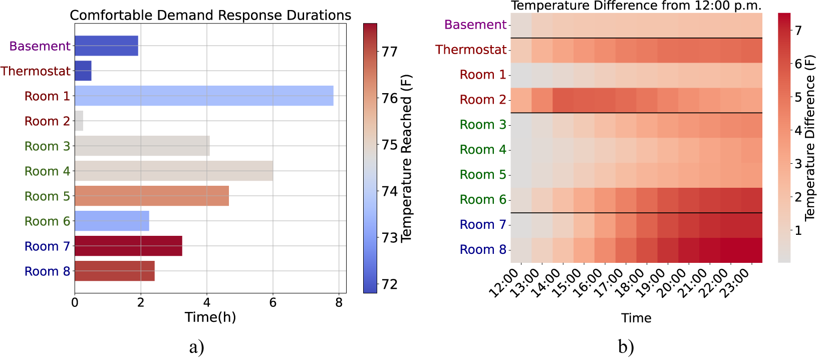
On June 19, 2023, we replicated a DR event at 12:00 pm on our entirely unoccupied Test bed 2, during which the average outdoor temperature was 85 °F. Figure 5a shows the comfortable DR duration (CDRD) (defined as the duration of time it takes for a room’s temperature to rise by 2 °F in the absence of cooling) for each room colored by the final temperature reached, providing a detailed view of how a DR event can differently affect comfort levels in various rooms. For example, Room 1 could maintain a comfortable temperature throughout an 8-hour DR event, whereas Room 2 could only do so for around 15 minutes. Moreover, Figure 5b illustrates the temperature increase over a 12-hour span, beginning at 12:00 p.m. Rooms are categorized and color-coded based on their location within the structure, arranged in ascending order. The distinct time intervals seen in each room’s temperature rise highlight the unique thermal behavior of individual spaces. For instance, Rooms 6, 7, and 8 reach their peak temperatures close to midnight, which may be a consequence of their specific orientation. Conversely, Room 2 experiences its peak temperature relatively early, likely attributable to its extensive window area. Room 1, on the other hand, displays a very small increase in temperature over a long period, which can be explained by its superior insulation.

Figure 5. A visual analysis of temperature shifts during a DR event, with the rooms distinctly color-coded and ordered on the y-axis to reflect their floor-level groupings. In Panel (a), a bar chart shows the elapsed time for temperatures to increase by 2 °F from noon across various rooms, while Panel (b) presents a heatmap depicting the temperature differential over time. Rooms situated on the same floor share color coding, and the sequence on the y-axis is arranged such that rooms on upper floors are positioned lower.

5.2.3. DR effects on ecobee DYD dataset

In order to validate that these discrepancies are not isolated to a single household but persist across larger samples, we expanded our analysis to residences fitted with five additional sensors during the cooling season (Section 3.3.3). We identified the FFPs, which are the periods between 12 pm and 5 pm when the outdoor temperature exceeds the indoor temperature for at least an hour. These intervals reflect typical DR events as the HVAC system remains off for substantial durations. However, it is worth noting that DR events happening during heatwaves could create larger discrepancies than we identified here. In each dwelling, the CDRD and temperature deviation from the initial temperature are computed. Table 1 shows the summary statistics considering all houses with a valid FFP. Fast-reacting rooms (FRRs) and slow-reacting rooms (SRRs) are defined as rooms that achieve their CDRDs the fastest or slowest compared to other rooms in the same household, respectively. We define the comfort gap as a pair of numbers showing the differences between the maximum and minimum (a) CDRDs and (b) temperature deviations within a house. These results indicate that, on average, the comfort gap among rooms in the same house is 52 minutes and 2.37 °F. Moreover, CDRDs can be 70% longer or 40% shorter than the duration of the room with the thermostat, on average. Further, distinct rooms can deviate from the thermostat reading by an average of 48% more or 34% less. The considerably large standard deviations underscore the substantial variability and distinctive thermal behavior of each house.

Table 1. Summary statistics of the CDRDs and temperature deviations of rooms during DR events

The analysis in this section highlights considerable variations in the performance of thermostats during operational and DR periods with significant discrepancies from setpoint values across different rooms in a house. It becomes evident that a single thermostat does not capture the temperature complexity of an SZMRH effectively.

7.1. Building thermal parameter identification

7.1.1. TTC (RC) identification

Utilizing the FFPs according to Section 3.2.1, we inferred the $ RC $ values for both cooling and heating seasons for each sensor-house pair. The subsequent process of outlier removal allowed us to infer suitable FFPs for 78.9% and 87.6% of the house-sensor pairs in the heating and cooling seasons, respectively. The increased success rate of thermal parameter identification during the cooling season could be attributed to the added parameter $ RQ $ , which introduces further flexibility to the process. The $ RC $ values we obtained show a good alignment with those reported in previous research (John et al., Reference John, Vallianos, Candanedo and Athienitis2018; Baasch et al., Reference Baasch, Wicikowski, Faure and Evins2019; Wang et al., Reference Wang, Chen, Li and Hong2021). This high rate of identification in our study is likely a result of our methodological choice to extract cooling and heating data over a nine-month period (Section 3.3.3). To display the benefit of considering a longer period, we replicated the cooling season analysis using a three-month summer period and found that utilizing a longer period improved the total duration of FFPs by 84%, which in turn resulted in a 21% improvement in the percentage of identified parameters.

The distribution of $ RC $ values for heating and cooling seasons is displayed in Figure 8. Each subfigure consists of two plots: the upper plot shows the collective distribution of $ RC $ values, while the lower plot presents the variances in room behavior within individual houses, color-coded by state. For instance, Figure 8a reveals an unimodal distribution of $ RC $ values, ranging from 1 to 27 hours for the cooling season. Contrarily, Figure 8b showcases a bimodal distribution for the heating season with a larger discrepancy in $ RC $ values ranging from 1 to 157 hours. The corresponding boxplot highlights intra-house differences as large as 20 and 143 hours among rooms for cooling and heating seasons, respectively. Given that $ RC $ values are solely dependent on the physical structure of the building, such variations between the $ RC $ values for summer and winter are unexpected. Yet, a similar discrepancy was observed in a prior study, which was attributed to the disparity in behavioral changes of occupants, such as a tendency to leave windows open more frequently during summer (John et al., Reference John, Vallianos, Candanedo and Athienitis2018). Additionally, the $ RC $ value for the room where the thermostat is located is marked with light blue for each house. If the room where the thermostat is located were to accurately represent the thermal behavior of the rest of the house, the marker would be positioned in the middle of each boxplot with a notably small range. However, the plot clearly shows that this is often not the case.

Figure 8. This histogram depicts the collective distribution of $ RC $ values (top), accompanied by boxplots for individual room distributions (bottom) for cooling and heating seasons. Markers indicated in light blue represent the $ RC $ values for the room where the thermostat is located.

In the heating season, there is a 30% chance that another room in the same house will have an $ RC $ value twice as high as the room with the lowest $ RC $ value. This probability slightly decreases to 24% during the cooling season. Furthermore, our analysis revealed that more than 50% of the time, a difference of 4 hours and 54 hours is observed in the $ RC $ values among rooms for the cooling and heating seasons, respectively.

7.1.2. $ RQ $ Identification

The identification of thermal $ RC $ values during the cooling season concurrently produces $ RQ $ values. The distribution of $ RQ $ values can be seen in Figure 9a. Upon conducting outlier and error filtering, 87.2% of the $ RQ $ values were successfully inferred. Our study reveals differences as significant as 3.2 °F among rooms within the same house (see Figure 9a). According to our findings, there is a 38% probability that one room will endure twice the solar heat gain compared to another room in the same house. Furthermore, there is a 25% likelihood that one room will experience three times the solar heat gain of its counterparts within the same dwelling. Despite lacking a concrete physical interpretation, these $ RQ $ values provide insightful data for retrofitting decisions, especially for identifying rooms that are most susceptible to high solar irradiance. Ultimately, the varied positions of the markers suggest that rooms with thermostats may experience notably less or more solar gain compared to other rooms within the same household. This wide range of outcomes underscores that thermostat measurements may inaccurately estimate the degree of solar gain across the household, with no discernible bias toward either lower or upper limits.

Figure 9. This histogram depicts the collective distribution of $ RQ $ and $ RK $ values (top), accompanied by boxplots for individual room distributions (bottom). Markers indicated in light blue represent the $ RK $ values for the room where the thermostat is located.

7.2. Interpretation of the parameters

After obtaining the $ RC $ , $ RK $ , and $ RQ $ values for each house, we carried out an independent analysis to identify homes with rooms that are at a high risk of having Poor Insulation, Low Solar Gain, High Solar Gain, and Low Heating Input. All comparisons were made based on the performance of other rooms within the same house. In order to identify rooms with deficiencies, we set certain assumptions. Rooms with $ RQ $ values one standard deviation below or above their mean are expected to face Low Solar Gain and High Solar Gain, respectively. Rooms exhibiting an $ RK $ value one standard deviation below the mean of the house are assumed to have Low Heating Input. Poor Insulation is first detected by analyzing $ RC $ data for both heating and cooling seasons by incorporating values that sit below one standard deviation from their mean. We then observed fewer houses with multiple rooms encountering Poor Insulation in the cooling season, whereas Poor Insulation from the heating season is more prevalent in houses but affects fewer rooms. This observation aligns with our initial assumption of lower $ RC $ values in the cooling season due to behaviors such as occupants leaving windows open more frequently. As a result, to accurately represent the actual physical attributes of the house, and not merely occupant behavior-related deficiencies, we define Poor Insulation using $ RC $ values from the heating season. It should be noted that since there are no studies that utilized the ST data for such purposes, there is no accepted metric for us to use. However, our approach is akin to the smart meter data-based inefficient house detection methodology conducted by Iyengar et al. (Reference Iyengar, Lee, Irwin and Shenoy2016). While this limited approach does not conclusively indicate such inefficiencies, it does help identify rooms with a high risk of such deficiencies.

Our observations indicate that a maximum of two rooms within a house exhibit such deficiencies. Although the actual number may be higher, this is a plausible estimate considering the constraints of having only six sensor readings from each house. Table 4 presents the number of houses exhibiting these deficiencies in just one room, two rooms, and the total. The percentages have been calculated based on the total data available for each instance separately, which explains why the denominator varies for each row. Overall, 96% of the houses exhibit High Solar Gain, with 78% in one room and 18% in two rooms. Low Heating Input emerges as the second most common deficiency, occurring in 85% of the houses overall, with 70% of the instances being confined to just one room. Low Heating Input is recorded in 78% of the houses, 69% of which observe it in only one room. Lastly, 70% of the houses are at risk of Poor Insulation, with 15% experiencing it in two rooms.

Table 4. Number of houses with deficiencies

In our final analysis, we examined the assumption that thermostat placements—ideally unaffected by vents or solar radiation—accurately represent overall house conditions. We computed the differences in thermal parameters across rooms from the room where the thermostat is located, with the summary statistics presented in Table 5. While the relatively low mean/median values might seem to initially endorse this assumption, the high standard deviations (shown by the coefficient of variance) indicate significant variation in each home’s thermostat-related behavior. This prevents us from drawing robust conclusions regarding the thermal conditions experienced by thermostats due to their physical locations. However, we can assert that they do not adequately represent the rest of the house.

Table 5. Statistical analysis of the thermal parameter difference of rooms from the thermostat

8.1. Explanatory data analysis

In our exploratory analysis, we augmented the ecobee DYD dataset with additional information from ecobee metadata, incorporating attributes like floor area and number of occupants. Although the ecobee DYD dataset lacks direct measurements of energy consumption, it includes the run time of cooling equipment as a feature. By aggregating the cooling run times for homes equipped with multi-stage cooling systems, we derived a consolidated feature termed “Cooling Run Time.” This metric serves as an indirect indicator of energy consumption during the cooling season. However, it is worth noting that this metric, while useful for estimating energy consumption, does not account for the varying energy usage rates associated with different operational stages in multi-stage systems. Figure 10a shows the distribution of the total cooling run time of houses for the summer season, colored by the number of sensors they have. As expected, we see a clear proportional relationship between the number of sensors and the total cooling time when the effect of the average outdoor temperature is removed. In terms of states, we see that only Texas has a similar trend to the one we see in outdoor temperature. However, when data are segmented by either floor area or number of occupants, the increase in sensor count does not significantly impact energy consumption, suggesting that these factors might play a minimal role in the observed energy usage patterns.

Figure 10. Panel (a) depicts box plots that categorize total cooling time by the number of remote sensors (0–5) across various household attributes such as state locations, average outdoor temperatures, floor area, and occupancy. Panel (b) presents cooling time per unit floor area as box plots, stratified by the same states and average outdoor temperatures, revealing how cooling efficiency correlates with the presence of remote sensors within the dwelling.

Acknowledging the potential for the binning of floor area to obscure its impact, we embarked on a secondary analysis. This involved the introduction of a new attribute, cooling run time per square foot, derived by dividing a house’s total cooling time by its floor area. Figure 10b presents this metric’s effects across different categorizations, namely, state and average outdoor temperature. This deeper dive reveals that, absent state-specific effects, there is no evident trend toward increased energy use. However, the analysis suggests an increase in energy consumption associated with a greater number of sensors when considering the intersection with average outdoor temperatures.

8.2. Statistical analysis

The exploratory data analysis has provided initial insights into the potential impact of additional sensors on energy consumption. Building upon these findings, we now aim to delve deeper by conducting a comprehensive statistical analysis. This offers empirical evidence concerning the correlation between sensor deployment and energy usage. Our methodology is inspired by the approach used by Barreca et al. (Reference Barreca, Clay, Deschenes, Greenstone and Shapiro2016), which explored the effects of temperature on mortality rates, adapting it to our context of energy consumption in residential settings.

To commence, the year-long dataset from ecobee’s DYD program was processed to obtain hourly data points. This resampling involved summing up the run time of both cooling and heating equipment for each hour, while temperature readings were averaged over the same period. Further, we computed a combined run time by summing cooling and heating run times. This allowed us to make claims related to the general energy consumption of the houses. We then calculated the Duty Cycle (unitless) for both cooling, heating, and combined run times by dividing the equipment’s run time (in seconds) by 3600 seconds, thus obtaining a ratio reflecting the proportion of time the HVAC system was operational within each hour. Additionally, the number of sensors at any given hour was determined by counting the number of non-null temperature readings from the remote sensors.

We have formulated our regression problem as follows:

(8.1) $$ {DC}_{it}=\sum \limits_{j=0}^5\left({\beta}_j\cdot {s}_{j, it}\times {T}_{it}\right)+{\alpha}_i+{\rho}_h+{\nu}_m+{\unicode{x025B}}_{it}, $$

where $ {DC}_{it} $ represents the heating, cooling, or combined duty cycle for house $ i $ at hour $ t $ .

$ {s}_{j, it} $ represents the presence of sensor count $ j $ for house $ i $ at hour $ t $ .

$ {T}_{ti} $ represents the outdoor temperature for house $ i $ at hour $ t $ .

$ {\beta}_j $ are coefficients for the interaction of $ {j}^{th} $ additional sensor dummy (as $ j $ goes from $ 0 $ to $ 5 $ ) with outdoor temperature $ {T}_{it} $ at hour $ t $ .

$ {\alpha}_i $ represents the fixed effects for each house, controlling for unobserved heterogeneity across houses.

$ {\rho}_h $ represents the fixed effects for each hour $ h $ of the day, controlling for diurnal variations.

$ {\nu}_m $ represents the fixed effects for each month $ m $ of the sample, controlling for time-varying patterns across the dataset.

$ {\unicode{x025B}}_{it} $ is the error term for house $ i $ at hour $ t $ .

The R environment is used to fit the models. The summary of the results of the model fit for the combined duty cycle can be found in Table 6. Our initial analysis on combined duty cycle demonstrates statistically significant results for each sensor’s impact on energy consumption. All coefficients being positive also implies that cooling is the dominant energy consumption. Furthermore, since remote sensors are often sold in pairs, our analysis indicates that users enhancing their ecobee premium system with a two-sensor pack can expect a 4.9% rise in energy usage per degree Fahrenheit change in outdoor temperature. Progressing from no extra sensors to a total of 5 can escalate cooling consumption by 17.8%.

Table 6. Statistical summary of the model evaluating the effect of sensor count and outdoor temperature on HVAC (combined) duty cycle (1/°F)

Note. Fixed-effects: id: 1000, hour: 24, and month: 12. Standard errors: clustered (id).

^a Signif. codes: 0’***’ 0.001’**’ 0.01’*’ 0.05’.’ 0.1” 1.

Figure 11 depicts the impact of a 1 °F increase in outdoor temperature on the total energy consumption, with brackets showing the 95% confidence intervals. The trend indicates that increasing the number of sensors results in increased energy consumption per degree change in the outdoor temperature. The largest jump with the addition of a sensor happens when switching from 0 to 1 with a 6.5% increase in demand. This finding gains significance with the introduction of newer ecobee thermostat models like the ecobee premium, which comes with an additional sensor. Furthermore, since remote sensors are sold in pairs, our analysis indicates that users enhancing their ecobee premium system with a two-sensor pack can expect a 4.9% rise in their energy usage per degree Fahrenheit change in outdoor temperature. Moving from no extra sensors to a total of 5 can escalate consumption by 17.8%.

Figure 11. Estimated impact of 1 °F in outdoor temperature on HVAC (combined) duty cycle. 95% confidence interval is shown using brackets.

The summary of the results of the two model fit for the heating and cooling duty cycle can be found in Table 7. For cooling, data clearly show a positive relationship between the number of sensors and energy consumption, with all coefficients from $ {\beta}_0 $ through $ {\beta}_5 $ being positive and statistically significant. This is an expected result since the increase in outdoor temperature would result in an increase in cooling energy consumption. Notably, the magnitude of these coefficients increases with each additional sensor, indicating that the addition of each sensor contributes to higher energy use. This consistent increase across sensor counts strongly suggests that the deployment of more sensors leads to significant increases in cooling energy consumption, likely due to the sensors capturing more spatial temperature variability and triggering more frequent or intense cooling responses.

Table 7. Statistical summary of the model evaluating the effect of sensor count and outdoor temperature on cooling and heating duty cycle (1/°F)

Note. Fixed-effects: id: 1000, hour: 24, and month: 12. Standard errors: clustered (id).

^a Signif. codes: 0’***’ 0.001’**’ 0.01’*’ 0.05’.’ 0.1” 1.

In contrast, the heating duty cycle presents a more complex picture. The coefficients for the number of sensors interacting with outdoor temperature show negative estimates with statistical significance. Negative values are expected due to the inverse relation between outdoor temperature and heating run time. This mixed outcome suggests a nuanced relationship where, under certain outdoor temperature conditions, increasing the number of sensors does not uniformly increase energy consumption for heating. In some cases, it might even reduce it, possibly due to optimized heating strategies facilitated by the data from these sensors or the stack effect helping with the rooms on upper floors.

The comparison of values in Table 7 shows that the coefficients for heating are significantly smaller, likely because there’s less need for heating over a narrower temperature range characteristic of warmer climates. Therefore, the model tends to identify smaller coefficients for heating consumption. This effect on the coefficients wouldn’t be present if the relationship between outdoor temperature and energy consumption were linear. However, given the exponential nature of this relationship, the temperature differential within warmer ranges of outdoor temperature leads to substantially smaller heating duty cycles. This outcome is anticipated, considering the dataset includes a significant number of houses from California, where cooling is often the primary energy demand due to the state’s warmer climate.

Figure 12 illustrates the influence of a 1 °F increase in outdoor temperature on the cooling (a) and heating (b) duty cycles, with brackets indicating the 95% confidence intervals. For cooling, the trend is almost identical to combined duty cycle, reinforcing the notion that cooling predominantly drives overall energy consumption. There is a discernible positive trend as the number of sensors increases. Notably, the transition from 0 to 1 sensor incurs a 6.4% uptick in energy consumption per degree change in outdoor temperature. Furthermore, we observe that users augmenting their ecobee premium with a two-sensor pack can cause a 4.8% rise in cooling energy usage per degree change in outdoor temperature. Lastly, the switch from no extra sensors to a total of 5 can surge the cooling consumption by 17.8%, which is identical to what was observed for combined energy consumption.

Figure 12. Estimated impact of 1 °F in outdoor temperature on (a) cooling and (b) heating duty cycle. 95% confidence interval is shown using brackets.

When switched to heating, a fluctuating correlation happens, as can be seen from 12(b). Generally, the coefficients decrease as the number of sensors grows. It is important to note that smaller negative coefficients indicate a larger reduction from the baseline consumption, leading to smaller energy consumption. We observe that having one additional sensor could reduce the energy consumption by 4.2% per outdoor degree change. Additionally, augmenting the existing ecobee premium thermostat (that already comes with an extra sensor) with two additional sensors can lead to a 14.1% decrease in heating demand. Surprisingly, we see that adding an additional sensor could result in a 25% reduction (from 2 to 3) or a 19% increase (from 3 to 4) in heating energy consumption. Lastly, the switch from not having any sensors to having 5 results in an 18.8% increase.

Recognizing the potential to uncover insights into how the impact of the number of sensors on energy consumption changes over time, we have identified seasonality as a critical factor for our analysis. This choice is driven by the hypothesis that the efficacy of sensors in influencing energy consumption could vary significantly across different seasons, due to variations in environmental conditions and heating or cooling needs.

To thoroughly investigate the influence of seasonality, we have reformulated our regression model to incorporate interactions between the number of sensors, outdoor air temperature, and the seasons. This revised approach allows us to examine how seasonal changes affect the relationship between sensor deployment and energy consumption.

(8.2) $$ {DC}_{it}=\sum \limits_{k=1}^4\sum \limits_{j=0}^5\left({\beta}_{jk}\cdot {SD}_k\times {s}_{j, it}\times {T}_{it}\right)+{\alpha}_i+{\rho}_h+{\nu}_m+{\unicode{x025B}}_{it}. $$

In the updated equation, denoted as Equation (8.2, two primary modifications have been made compared to Equation (8.1. First, we introduced $ {SD}_k $ , representing the dummy variable for the $ {k}^{th} $ season, to our model. Second, the dummy variables for the number of sensors now encompass the scenario of having zero additional sensors, which previously served as the baseline in Equation (8.1. The inclusion of the zero additional sensor condition in our current analysis aims to elucidate the seasonal effects on scenarios where no extra sensors are used.

The outcomes derived from Equation (8.2) are detailed in Table 8. Notably, with the exception of $ {\beta}_{5: Summer} $ in the heating analysis, all results exhibit statistical significance. This underscores a clear correlation between the number of sensors and heating usage, particularly when the influence of seasonality is considered.

Table 8. Statistical summary of the model evaluating the effect of sensor count, outdoor temperature, and seasonality on cooling and heating duty cycle (1/°F)

Note. Fixed-effects: id: 1000, hour: 24, and month: 12. Standard errors: clustered (id).

^a Signif. codes: 0’***’ 0.001’**’ 0.01’*’ 0.05’.’ 0.1” 1.

Figure 13 demonstrates the estimated impact of a 1 °F increase in outdoor temperature on a) cooling and b) heating duty cycles across different seasons. For cooling energy consumption, our results align with anticipated trends, revealing a pronounced increase in cooling run time during the summer months. The distinction between autumn and spring is minimal, with spring presenting slightly lower cooling usage. Winter sees the smallest effect, yet the overall ascending trend observed in Figure 12a persists, especially during summer, when cooling demand rises with each additional sensor.

Figure 13. Estimated impact of 1 °F in outdoor temperature on (a) cooling and (b) heating duty cycle for each season. 95% confidence interval is shown using brackets.

The heating analysis presents a more variable pattern. In this context, a downward shift in heating duty cycle values indicates a decrease in heating expenses. The analysis reveals that incorporating just one additional sensor can reduce heating equipment use by 4.4%. However, expanding an ecobee premium by adding a pack of remote sensors (transitioning from 1 to 3 sensors) leads to a 3.6% increase in heating expenses. Collectively, these findings suggest that the inclusion of extra sensors has a marginal impact on heating energy consumption. This aligns with prior observations regarding the smaller temperature disparities during the heating season, as depicted in Figure 7. Such phenomena were attributed to the stack effect and the roles of internal and solar heat gains in maintaining indoor temperatures. Additionally, unaccounted space heaters might have contributed to this phenomenon.