


1. Introduction
Glaciers in Alaska have been losing mass at an accelerating rate and are projected to be among the highest contributors to global sea level rise in the next 100 years (Edwards and others, Reference Edwards2021; Hugonnet and others, Reference Hugonnet2021) due to forcings linked to anthropogenic climate change. However, tidewater glaciers, which contain 57% of global ice volume excluding the Greenland and Antarctic Ice Sheets (McNeil and others, Reference McNeil2021), typically go through a sequence of advance, retreat and stability that is out of sync with these climate forcings (Pfeffer, Reference Pfeffer2007) as they have additional influences on their behaviour such as sediment transport, ablation and calving (Brinkerhoff and others, Reference Brinkerhoff, Truffer and Aschwanden2017; Amundson and Carroll, Reference Amundson and Carroll2018). This leaves more uncertainty on the rate of mass loss for individual tidewater glaciers, especially on the retreat phase of their cycle where they are vulnerable to a number of marine-related processes such as submarine melting and calving, which vary in importance at different locations (Truffer and Motyka, Reference Truffer and Motyka2016; Błaszczyk and others, Reference Błaszczyk2021).
Taku Glacier (T'aakú Kwáan Sít'i) is the largest glacier within the Juneau Icefield and is also a tidewater glacier. While most other glaciers in the Juneau Icefield have been thinning and retreating since the late 19th century, the Taku has been advancing or stable (Molnia, Reference Molnia2007). However, the most recent period of advance ended in 2018 (McNeil and others, Reference McNeil2021) when the Taku began to retreat for the first time since 1890 (Molnia, Reference Molnia2007), marking the beginning of a new phase in its tidewater glacier cycle. During its advance, the Taku has moved a large amount of sediment to its terminus allowing a shoal to be built up at the front of the glacier, which is currently protecting it from ocean water (Motyka and others, Reference Motyka, Truffer, Kuriger and Bucki2006). As the retreat phase begins, the Taku will no longer be able to maintain this shoal which will eventually allow ocean water to reach the terminus of the glacier (Post and others, Reference Post, O'Neel, Motyka and Streveler2011; Brinkerhoff and others, Reference Brinkerhoff, Truffer and Aschwanden2017), the base of which is below sea level. When this occurs, there is likely to be a more rapid retreat as the glacier is subject to the influence of calving and melting in water (e.g. Brinkerhoff and others, Reference Brinkerhoff, Truffer and Aschwanden2017). Once ocean influence on melting begins, a retrograde slope will lead to a positive feedback as an increasing amount of ice is exposed to ocean influence as the terminus moves inland (Frank and others, Reference Frank, Åkesson, De Fleurian, Morlighem and Nisancioglu2022). Once this positive feedback has started there are a number of geometric features that could slow and potentially stabilise the retreat such as bedrock bumps and glacier-width change (Mercer, Reference Mercer1961; Pfeffer, Reference Pfeffer2007; Catania and others, Reference Catania2018; Frank and others, Reference Frank, Åkesson, De Fleurian, Morlighem and Nisancioglu2022). There are studies of bed elevation on the Taku at limited locations (Fig. 1). The most extensive of these studies indicates the Taku occupies an overdeepened basin, hence the initial retreat will be on a retrograde slope, and that the bed elevation rises above sea level between 30 and 40 km upstream of the terminus (Nolan and others, Reference Nolan, Motkya, Echelmeyer and Trabant1995). However, the localised nature of the previous work means no bedrock bumps have been resolved and additionally the exact location where the bed rises above sea level has not been identified. This information gap hinders predictions of how the retreat of the Taku will proceed.
Study area map. (a) Map of Taku Glacier with locations of geophysical surveys, previous studies in orange, this study in green. Note that Profile 4 has been surveyed previously and in this study. The tributary branches (Matthes, Demorest, Northwest and Southwest) are labelled. Background in glacierised areas is the ice-surface velocity from NASA MEaSUREs ITS_LIVE project (Gardner and others, Reference Gardner, Fahnestock and Scambos2019). Brown shows ice free areas. Black box shows location of Fig. 2. Coordinates shown here and used throughout this paper are in NAD83 UTM 8N. (b) Map of Juneau Icefield with location of (a) shown in black outline.

Bed elevation of glaciers is commonly measured over large areas by radio-echo-sounding techniques. On the Taku, these have been unsuccessful in areas of thick ice due to the high radio-wave attenuation by temperate ice, causing bed echos to not be returned. In this study, we instead employ ground-based gravity measurements to estimate the bed elevation. The gravity method has been used to determine ice and sediment thickness in multiple other studies (e.g., Kanasewich, Reference Kanasewich1963; Casassa, Reference Casassa1987; Bandou and others, Reference Bandou2022) and has the advantage of a relatively lightweight field operation compared with other geophysical methods such as seismic methods.
Here we improve on estimates of the geometry of the bed of Taku Glacier, both in the across-flow and along-flow directions. Relative gravity measurements were made in the 2023 summer field season on two across-glacier profiles and one along-flow profile ~30−40 km upstream of the terminus. The ice thickness and the glacier geometry are modelled by the inversion of the gravity measurements in 3D rather than in 2D as is often done on valley glaciers (Kanasewich, Reference Kanasewich1963; Casassa, Reference Casassa1987) and outlet glaciers of ice sheets (Boghosian and others, Reference Boghosian2015). We introduce an approach where we construct a 3D model with limited data extent using a range of glacier-valley shapes that are often seen in landscapes that are currently covered by ice (glacierised) and were previously covered by ice (glaciated). Our new estimates on the glacier geometry show features that are likely to influence the future retreat rate of the Taku.
2. Study area
The Juneau Icefield covers a ~4000 km2 area extending from just north of Juneau, Alaska into British Columbia, Canada. Taku Glacier is the largest glacier draining the Juneau Icefield, at 56 km long and 725 km2 in area (McNeil and others, Reference McNeil2020). The native name for the Taku is T'aakú Kwáan Sít'i which translates to T'aakú People's Glacier with T'aakú meaning Flood of Geese (Southeast Native Subsistence Commission Place Name Project, 1994–2001; Zechmann and others, Reference Zechmann, Truffer, Motyka, Amundson and Larsen2021). This name originates from the Tlingit people whose ancestral lands include this region. The glacier has 4 branches (Matthes, Demorest, Northwest and Southwest), which converge to form the main branch (Fig. 1). We note an inconsistency in literature here as Nolan and others (Reference Nolan, Motkya, Echelmeyer and Trabant1995) refers to the Matthes and Demorest as separate glaciers, whereas McNeil and others (Reference McNeil2020) refers to them as branches of the Taku. Randolph Glacier Inventory 7.0 (RGI 7 Consortium, 2023) classifies the Taku as the Matthes, Northwest, Southwest and main branch (RGI2000-v7.0-G-01-19709) with the Demorest branch separated into Hole-in-the-Wall Glacier (RGI2000-v7.0-G-01-19712) and an unnamed glacier (RGI2000-v7.0-G-01-19713). We choose to follow the naming convention of McNeil and others (Reference McNeil2020) and refer to Taku glacier to include all of the branches (outlined in red in Fig. 1).
The surface of the Taku has been extensively studied as part of the Juneau Icefield Research Program (JIRP), which has established a naming convention for surface-elevation profiles that have been surveyed over a number of decades and we follow their naming convention here. JIRP operates out of a number of camps across the icefield. For this study, fieldwork was based out of Camp 10 and covered Profiles 4, 7a, and a section of Longitudinal A (Long A) (Fig. 1) extending from the main branch upstream into the Matthes Branch.
The Juneau Icefield lies within the Coast Mountains Complex (CMC), part of the North American Cordillera, which runs along all of the Coast Mountains in Southeastern Alaska and British Columbia (Drinkwater and others, Reference Drinkwater, Brew and Ford1995). The CMC formed in the late Cretaceous as part of a collision and accretion event between the Alexander-Wrangellia Terrane to the west and the Stikine Terrane to the east (Brew and Morrell, Reference Brew and Morrell1983). Crustal thinning allowed widespread intrusion of plutonic bodies and contact metamorphism. The resulting geology can be divided into northwest-trending belts and sub-belts defined by their composition and metamorphic grade. These can be broadly described as a central granitic zone with decreasing metamorphism moving away from this zone to the east and west (Brew and Morrell, Reference Brew and Morrell1979, Reference Brew and Morrell1983; Stowell, Reference Stowell2006). The majority of the Juneau Icefield lies within the central granitic zone and from the eastern side of the icefield moving towards the coast, the rock type shifts to more metamophic belts. The rocks within the study area are predominantly granodiorite and gneiss with increasing amounts of granodiorite to the east and increasing gneiss to the west (Brew and Morrell, Reference Brew and Morrell1979). There are no measurements of the density of the rocks in the area but the rock types indicate the likely range is 2670–2730 kg m−3 (Smithson, Reference Smithson1971; Christensen and Stanley, Reference Christensen and Stanley2003).
3. Previous studies
Most studies of Taku Glacier have relied on surface observations, including remote sensing and ground-based methods such as mass-balance pits and ablation stakes. Observations of the environment beneath the ice are much more limited. Geophysical surveys on the Taku are summarised in Table 1. Many of these are in the form of JIRP internal reports, which are not peer reviewed. The most comprehensive peer reviewed study is Nolan and others (Reference Nolan, Motkya, Echelmeyer and Trabant1995) who derived ice-thickness estimates from four cross sections across the glacier using active-source seismic and radio-echo sounding methods. They found the thickest ice (1477 m) and the deepest bed (617 m below sea level) at the Goat Ridge profile (Fig. 1).
Geophysical studies on the Taku
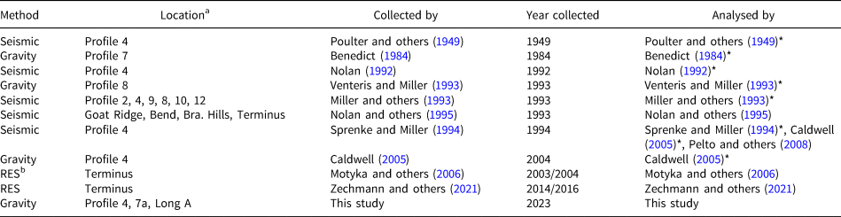
Note some datasets are used in multiple studies.
*Studies that are in non-peer-reviewed reports.
aProfiles shown in Fig. 1.
bRES = Radio-echo-sounding.
The most repeated survey location is Profile 4, where seismic and gravity surveys have previously been conducted. Seismic surveys on Profile 4 were carried out in 1992 and 1994, results from which can be found in the JIRP internal reports of Miller and others (Reference Miller, Benedict, Sprenke, Gilbert and Stirling1993) and Sprenke and Miller (Reference Sprenke and Miller1994). The seismic sections from Sprenke and Miller (Reference Sprenke and Miller1994) were digitised and reanalysed by Caldwell (Reference Caldwell2005), deriving a glacier cross section with a V-shaped bottom and maximum depth of 400 m below sea level. Caldwell (Reference Caldwell2005) also carried out a gravity survey across Profile 4, the results of which showed a smoother U-shaped valley rather than a V-shape, with the maximum ice thickness about 200 m less than that derived from the seismic surveys. At the upstream end of our measurements is Profile 7, which has been previously studied with a gravity survey (Benedict, Reference Benedict1984). However, the surface elevations used for the their gravity-data processing were derived from a topographic map rather than being measured in situ, leaving considerable uncertainty on the resulting ice-thickness and bed-elevation estimates and therefore we do not use these results in our analysis.
Ice thickness of glaciers worldwide, including the Taku, have been estimated by Farinotti and others (Reference Farinotti2019) and Millan and others (Reference Millan, Mouginot, Rabatel and Morlighem2022), both using the inversion of surface characteristics such as the slope and velocity. The estimates from Millan and others (Reference Millan, Mouginot, Rabatel and Morlighem2022) contain many data voids in our study area, so we choose to not use these in our analysis. Farinotti and others (Reference Farinotti2019) estimates the maximum thickness across Profile 4 on the Taku is 950 m and the deepest point of the bed here is 250 m above sea level. This is significantly less ice than seismic methods suggest, indicating the assumptions used in the surface-characteristics-inversion methods do not hold true for the Taku. Therefore, the results from methods such as these can not be used to reliably map the bed elevation, indicating the need for more in situ geophysical studies.
4. Methods
4.1 Data collection and processing
Gravity measurements were made using the Scintrex CG-5 Autograv gravity meter in June 2023. The survey was carried out as a relative gravity survey, with measurements recorded relative to the local base station established on an exposed rock surface at Camp 10. Measurements were taken at the Camp 10 base station twice a day to determine the instrument drift over the whole survey period. At each measurement location, the gravity meter was set on the snow with its base on a wooden board. The instrument was levelled and four ten-second measurements were recorded at a sampling rate of 6 Hz then averaged. Accurate location and elevation of each measurement point was determined by the Post Processed Kinematic technique using two Emlid Reach RS2+ dual-frequency GNSS receivers. Base station positions were processed from raw satellite-observation data using the Canadian Spatial Reference System Precise Point Positioning service. Gravity measurements were made over four days in clear, calm weather conditions with movement between stations on skis. A total of 43 locations were surveyed, six of which were visited twice for repeat measurements to determine the uncertainty (Fig. 2).
Location of model domains and measurements. (a) Inactive model domain, with the ice thickness from Farinotti and others (Reference Farinotti2019). Location of the active model domain shown in orange outline and black box denotes location of (b). (b) Active model domain, with locations of gravity measurements and centre points. Background in both (a) and (b) is the hillshade image of the ArcticDEM surface elevation at 2-m resolution (Porter and others, Reference Porter2023).

Gravity measurements were first corrected for earth tide using the method of Longman (Reference Longman1959) and then for latitude following International Gravity Formula 1980. A linear function was then fit through the earth-tide- and latitude-corrected gravity values at the local base station to determine the instrument drift. The drift averaged 1.3 mGal per day and once the linear-drift function was determined and removed the measurements at the base station showed a standard deviation of 0.07 mGal. This linear function was then used to correct drift on all measurements based on the date and time they were recorded. Free-air anomalies were calculated by applying the free-air correction (e.g., Long and Kaufmann, Reference Long and Kaufmann2013).
The Bouguer anomaly was calculated using the Bouguer slab correction with the elevations measured in the field and a density of 2700 kg m−3. This density was deemed appropriate based on the geology of the area (section 2). A terrain correction was also required due to the steep sides of the valley walls, which cause an additional contribution to the gravity anomaly not accounted for with the slab correction. For the terrain correction, we calculated the gravity contribution of the terrain using 3D modelling in Fatiando a Terra, an open-source Python geophysical modelling and inversion library (Uieda and others, Reference Uieda, Oliveira and Barbosa2013). This method creates vertical rectangular prisms between the defined surface and a reference elevation. The gravity contributions from each of these prisms is then calculated using the method of Nagy and others (Reference Nagy, Papp and Benedek2000, Reference Nagy, Papp and Benedek2002). The ArcticDEM Digital Elevation Model (DEM) mosaics (Porter and others, Reference Porter2023) regridded at 100-m resolution were used to define the terrain. The terrain correction was then subtracted from the Bouguer anomaly to give the terrain-corrected Bouguer anomaly. This is the anomaly we use for modelling throughout this study and hereafter refer to simply as the Bouguer anomaly. Note that because we will be using this Bouguer anomaly to model the ice thickness, it does not include any contributions from the ice.
The Bouguer anomaly obtained after the corrections includes contributions from the long-wavelength regional anomaly caused by variations in crustal structures, local variations in basement rock density, and the negative density contrast of the glacier (Casassa, Reference Casassa1987). In our study area, the regional Bouguer-anomaly field (Bonvalot, Reference Bonvalot2012) does not show a trend that is distinct from ice-thickness variations across the area. As such, we determine any potential contributions from crustal structures and regional geology to be minimal in comparison to the signal from the ice and therefore we use the Bouguer anomaly as described above.
4.1.1 Measurement uncertainty
The uncertainty on individual gravity measurements is calculated as a root sum squared (RSS) of the uncertainty from the correction elements. We do not include a contribution from the uncertainty in the earth-tide and latitude corrections as the uncertainty of the latitude measurements is deemed sufficiently low to not affect the overall uncertainty (Muto and others, Reference Muto, Christianson, Horgan, Anandakrishnan and Alley2013b). The uncertainty on the drift-corrected gravity anomalies is calculated using the standard deviation in the measurement at each location and the standard deviation on the base-station measurements. The uncertainty on the free-air and Bouguer anomalies is calculated by using the uncertainty of the elevation measurements, propagated through the free-air and Bouguer corrections. The uncertainty on the terrain correction is estimated by finding the standard deviation of 100 runs of the terrain correction with density randomly selected from the expected range (section 2) and the elevation perturbed with a normal distribution with a standard deviation of 1 m. The RSS of these elements results in a mean uncertainty of 0.08 mGal at the measurement locations. The maximum repeat measurement difference is 0.15 mGal, which occurs at a point measured at the start and end of the day on Profile 4. We chose to take a conservative approach to the uncertainty and take the RSS of this maximum repeat measurement difference with the measurement uncertainty to give the total uncertainty at each measurement point, resulting in a mean value of 0.17 mGal.
4.2 Modelling approach
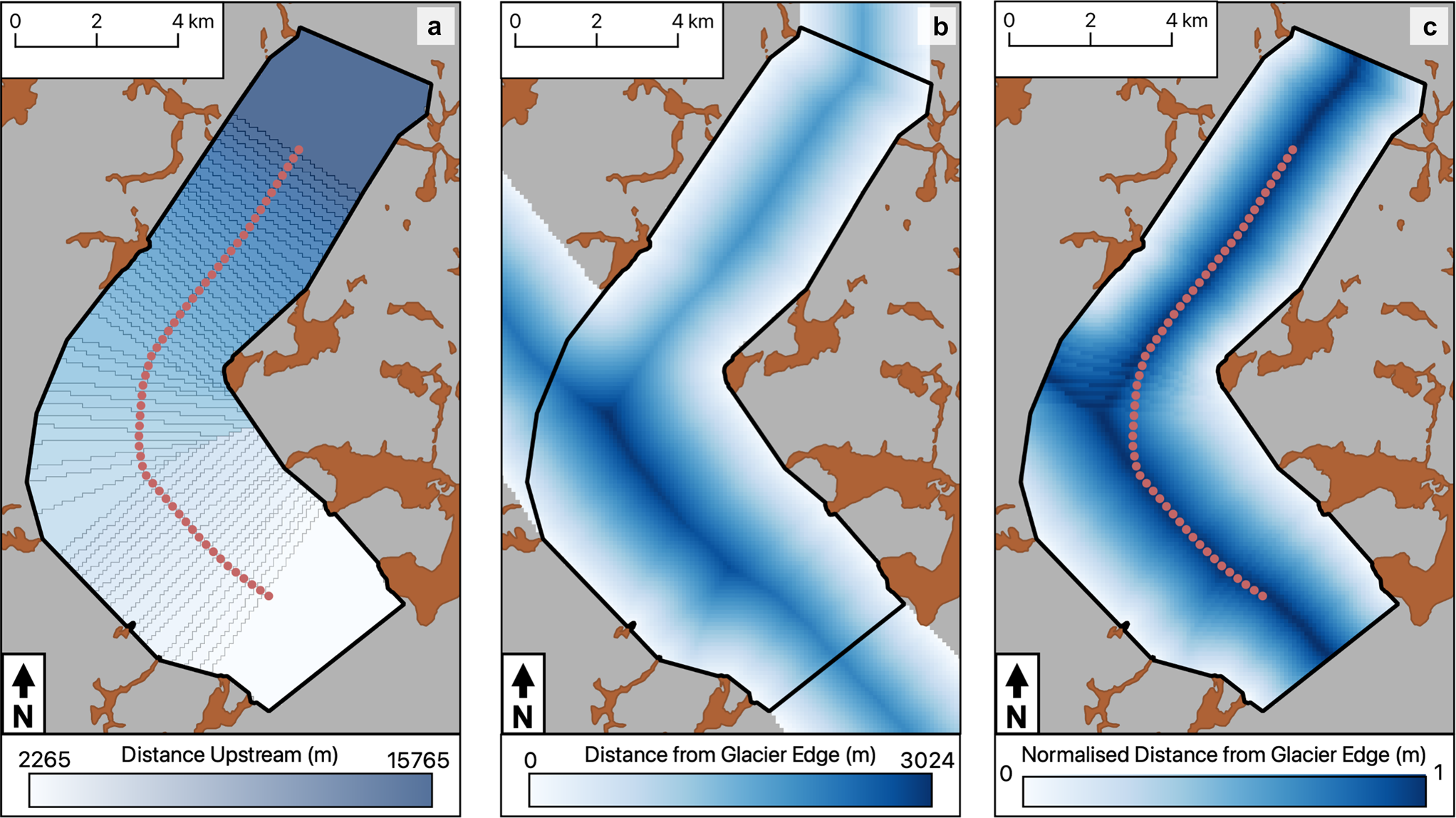
Valley glaciers are often modelled in 2D when across-glacier measurements are available, as in our case, because their long, straight geometry can be approximated by the 2D across-glacier shape extending infinitely in the direction of the glacier flow and perpendicular to the line of measurements. However, our initial modelling of the Taku in 2D showed that this approach is not valid because the width of the glacier varies, there is a curve in the area of our measurements and there are numerous small side basins and tributaries joining the main branch. Therefore, we model the glacier in 3D. The data availability is not extensive enough to allow a full 3D gravity inversion without constraints on the glacier shape. Hence, we define a method that allows a fixed glacier-valley shape to be applied across the whole study area. To do this, we first define an active model domain in which we will model the ice thickness, then divide this domain into bands that will each have a different maximum ice thickness (Fig. 3a). To apply a glacier shape, we calculate the distance from nearest glacier edge for each point in the active model domain and then normalise these values within each of the domain bands (Figs. 3b,c). This allows a glacier valley shape, such as V- or U-shape, to be applied across the whole active model domain with a different maximum thickness in each of the bands.
Components of the method for applying the glacier shape in the 3D gravity modelling. Areas in brown indicate exposed rocks and grey background shows glacier areas excluded from the modelling process. Active model domain is outlined in black. (a) Distance bands with distance upstream applied by which centre point the grid cell is closest to. Centre points used to define the bands are shown as pink dots. Edges of bands are outlined in grey lines. (b) Distance from the nearest glacier edge. Glacier edge here is defined to not include small side basins and tributaries but includes continuation of the Taku main branch to the northwest. (c) Distance from the nearest glacier edge normalised by the maximum distance within each of the distance bands.
4.2.1 Model domain
The model domain is split into two subsections, the active model domain and the inactive model domain. The active model domain is where we model the ice thickness through the inversion of our gravity data and we define it to include the central region within the glacier trunk where the measurements are located and exclude side basins with slow-flowing ice (typically below 10 m a−1). This domain is extended 3 km upstream and downstream from the ends of the Longitudinal A profile to minimise the edge effect (outlined in orange in Fig. 2). The active model domain is discretised into 100 × 100-m grids. In this simplified active model domain, we do not include side basins or tributaries as we do not have any data to constrain the ice thickness in these areas. However, the gravity contribution from ice outside the active model domain must also be accounted for. We include this contribution from the inactive model domain by calculating the gravity anomaly from glaciers within 45 km of our measurement points using the ice thickness from surface-inversion methods (Farinotti and others, Reference Farinotti2019). Although these methods underestimate the ice thickness at Profile 4 compared to the seismic measurements (section 3), we assume that it is a reasonable estimate in areas outside of the main trunk of the glacier which are farther away from the measurement points and have shallower ice. We later assess the sensitivity of our modelling approach to the potential ice-thickness variations in the inactive model domain (see section 5.1). Not including the contribution from ice outside the active model domain would lead to underestimating the ice thickness, and is likely why the gravity derived ice thickness results from Caldwell (Reference Caldwell2005) are shallower than those estimated from seismic measurements. The calculated gravity from the inactive model domain remains constant throughout our method as we are not varying the ice thickness in these areas. Therefore, we make a single calculation of this effect and sum it with the modelled gravity from the active model domain to give the total gravity anomaly. The ice thickness from both the active and inactive model domains is subtracted from the ArcticDEM surface topography (Porter and others, Reference Porter2023) to give the bed topography and allow calculation of gravity anomaly from the full ice column.
4.2.2 Distance bands
We divide the grid cells in the active model domain into across-glacier bands to allow the ice thickness to vary along flow and glacier shape to be applied at different glacier widths. To assign each grid cell to a distance band, we first define a line of points along the centre of the active model domain at 250-m intervals (pink dots in Fig. 2), each with an associated distance from the downstream end of the active model domain. Each grid cell in the active model domain is then assigned the same distance value as the centre point to which it is closest. In this way, bands are formed by groups of grid cells being assigned the same distance values (Fig. 3a).
4.2.3 Distance from Glacier edge
The glacier shape is applied within the active model domain by defining the ice thickness as a function of distance from the glacier edge. To assign the shape for each cell in the active model domain, we calculate the distance from the nearest glacier edge. For this calculation, small tributaries are again excluded but the continuation of the main branch of the glacier to the northwest is included to allow the glacier shape to be represented where the active model domain curves across this region (Fig. 3b). Using the absolute value of the distance from the glacier edge to define the shape would lead to truncation of the form between areas which have different maximum distance values in the centre of the glacier. Therefore, we normalise the distance from the glacier edge within each of the distance bands to ensure the full shape is applied in each of them (Fig. 3c).
4.2.4 Ice thickness
We convert the normalised distance from glacier edge to normalised ice thickness by defining a relationship between the normalised distance and normalised ice thickness for the valley shape we want to apply. For example, a V-shaped valley profile would be defined by a linear relationship between distance from glacier edge and ice thickness. We use the defined valley shape relationship to calculate a value of normalised ice thickness for each grid cell in the active model domain. The map of normalised ice thickness allows the ice thickness across the whole active model domain to be varied by just changing the applied maximum ice thickness. We allow the ice thickness to vary across the active model domain by applying a different maximum ice thickness in each of the distance bands.
4.3 Simple-shape inversion
Our gravity measurements include two across-glacier profiles and one along-flow profile (Fig. 2). The across-glacier profiles can give an indication of the shape of the glacier at these locations but the shape between these profiles is unknown and cannot be constrained well with available data. Therefore, we must make an assumption about the shape in these areas to model the glacier in 3D. We first conduct the gravity inversion for the whole domain with a few simple valley shapes, within which we expect the true shape to lie. For these inversions, the across-glacier shape is kept constant along the entire glacier length within the active model domain and only the ice thickness along flow is allowed to vary. In this approach, only the gravity measurements along the Longitudinal A profile are used to assess the model fit as the across-glacier profiles do not help constrain the ice thickness as the glacier shape is not allowed to vary.
4.3.1 Valley shape
The shape of many glacier valleys can be approximated with a power-law model (e.g., James, Reference James1996; Li and others, Reference Li, Liu and Cui2001) of the form:

where D is the maximum glacier depth, W is the half width and a and b are constants. The exponent b describes the shape of the profile with b = 1 defining a V-shaped profile and b > 1 a parabolic, U-shape profile where the width of the U-shape increases with increasing b value. Studies of glacierised and glaciated valley shapes show many glacier troughs can be modelled with b between 1 and 2.8 (e.g., Li and others, Reference Li, Liu and Cui2001; Brook and others, Reference Brook, Kirkbride and Brock2004; Benn and Evans, Reference Benn and Evans2013). To provide a range of results within which we estimate the true model is likely to lie, we model the glacier shape with b equal to 1 (V-shape), 2 (U-shape) and 2.8 (wide-U-shape) (Fig. 4). A simplifying assumption we must make with this method is that the thickest ice will be at the greatest distance from the glacier edge.
Normalised distance from glacier edge to normalised ice thickness relationships for valley geometries used in simple shape inversions.

4.3.2 Gravity inversion
We carried out the gravity inversion using Very Fast Simulated Annealing (VFSA), which has been applied to glaciological problems by several previous studies (e.g., Roy and others, Reference Roy, Sen, Blankenship, Stoffa and Richter2005; Muto and others, Reference Muto, Anandakrishnan and Alley2013a, Reference Muto, Christianson, Horgan, Anandakrishnan and Alley2013b, Reference Muto2016). Our implementation of the VFSA algorithm is similar to Muto and others (Reference Muto, Anandakrishnan and Alley2013a, Reference Muto, Christianson, Horgan, Anandakrishnan and Alley2013b), so readers are referred to them for the details, Here, we note the three key differences: (1) in this study, we use the terrain-corrected Bouguer anomaly instead of the free-air anomaly; (2) the forward gravity-anomaly calculation uses the method of Nagy and others (Reference Nagy, Papp and Benedek2000, Reference Nagy, Papp and Benedek2002) as implemented in Fatiando a Terra (Uieda and others, Reference Uieda, Oliveira and Barbosa2013); and (3) we ran VFSA 100 times until the algorithm reached the tolerance, i.e. the misfit between the measured and the modelled gravity anomaly fell below the level expected by the measurement uncertainty, and the mean of the resulting 100 models was calculated as the most likely model with the 95% confidence interval as the model uncertainties.
In each VFSA run, the model is perturbed by varying the maximum ice thickness for each distance band. This is done by varying the ice thickness along the points in the centre of the model area (pink dots in Fig. 2), each of which correspond to a distance band. It is important to note that these centre points do not represent the point of maximum ice thickness within each band, that is determined by maximum distance from a glacier edge. The ice thickness at the centre point is converted to a value for maximum ice thickness, which is then applied to the whole band. The centre points all have a starting ice thickness of 1550 m as this is the maximum value of ice thickness from previous seismic measurements at Profile 4. We do not use the seismic measurements to constrain the model in any other way, but we found that the starting thickness within a reasonable range does not affect the final model result. The ice thickness at the centre points is allowed to vary between 950 and 1950 m. We used 917 kg m−3 as the density of ice and 2700 kg m−3 as the density of bedrock, which were determined based on the average density of temperate ice and the geology in the area, respectively.
We design the inversion to only perturb over small areas where the misfit is greater than the tolerance, which results in faster model convergence. At each iteration of the inversion process, a distance band is selected at random and the selected band and those within 500 m of it are perturbed. A smoothing function is applied after each model perturbation to reduce unrealistically large changes in the ice thickness over small distances. This smoothing is applied to model grid cells in distance bands within 750 m of each of the perturbed band and by applying a weighting of 4, 1, 1 at distances of 0, 200, 750 m, respectively. The weighting and distances were chosen to be the smallest possible while still reducing large jumps in ice thickness. After the model perturbation, forward calculation of the gravity anomaly is executed and the misfit is assessed at the three measurement points closest to the randomly selected distance band. Subsequent perturbation is carried out only if the misfit over those three points is higher than the tolerance. The acceptance of the perturbed model is also assessed at these three points.
4.4 Manual fitting for across-glacier shape
Using the results from the simple-shape inversions, we calculate the gravity anomalies along the across-glacier profiles. This reveals misfit across these profiles that indicates the departure of the glacier valley from the simple shapes used. Additionally, the misfits are different at each of the across-glacier profiles, which shows that the valley shape changes along the active model domain. We attempted to derive an inversion scheme to model valley shapes more complex than the simple U- or V-shapes. This proved difficult because when the same shape was applied across the whole active model domain, the inversion will return a valley shape which is a best fit at both across-glacier profiles. However, this best fit model then fails to reach tolerance as the misfit cannot be reduced enough at either of the profiles while trying to satisfy the other. In an inversion scheme where the shape is different across the active model domain, we need to assume where the shape change occurs. In testing such schemes, we found that the along-flow ice thickness depends on the location of the shape change that cannot be constrained sufficiently.
For these reasons, we instead further reduce the misfit at the across-glacier profiles by manually altering the valley shape. We do this at each across-glacier profile separately by varying the shape and ice thickness within a 2 km buffer zone of each profile. The ice outside this 2 km zone will still contribute to the total gravity anomaly at each across-glacier profile. Therefore we create three separate manual-fit models for each of the simple-shape-inversion glacier shapes. Within the 2 km manual fit zone, the valley-geometry and ice thickness can be manipulated freely but beyond this zone, the geometry is held as either V-shaped, U-shaped or wide-U-shaped and the ice thickness is assigned as the mean from the associated simple-shape inversion.
This manual-fit method allows us to refine the geometry to show a range of potential shapes at the two across-glacier profiles with an improved fit over the simple-shaped geometries. These manually-fitted geometries cannot be applied across the whole active model domain as we do not have any additional across-glacier profiles to refine the shape along flow. However, they give an insight to which of the simple-shape models is the most likely at each of our across glacier profiles and therefore which of the simple-shape models is the most applicable across the whole active model domain.
5. Results
5.1 Simple-shape inversion
The simple-shape inversions produce results with varying maximum ice thickness. This can be seen in the blue lines in the along-flow profile (Fig. 5a) and the two across-flow profiles (Figs. 6b and 7a). The maximum ice thickness and root mean squared (RMS) error at Profiles 4, 7a and Longitudinal A for each of the model versions is shown in Table 2. The b = 1 (V-shape) model produces the the greatest ice thickness across all profiles. The b = 2 (U-shape) and b = 2.8 (wide U-shape) models produce results that are both less than the V-shape model but differ relative to each other at Profiles 4 and 7a. At Profile 7a, the wide-U-shape model has a similar maximum thickness to the U-shape model. Whereas at Profile 4, the wide-U-shape model has a greater maximum thickness than the U-shape model. These variations show a general trend of increasing maximum ice thickness with decreasing value of b (more V-shaped) that is related to the change in the cross-sectional area of the different glacier-valley shapes. The anomaly to this trend is where we see an increase in the maximum ice thickness at Profile 4 between the U-shape and wide-U-shape models. This is likely because the measurements are relative to Camp 10, which is at the east side of Profile 4, and the wide-U-shape is increasing the amount of ice close to Camp 10, therefore requiring an increase in ice thickness to produce the same difference in gravity between Camp 10 and the centre of the glacier. The different shapes and ice thicknesses between models result in varying area below sea level. Despite producing the largest maximum ice thickness, the V-shape model produces only a narrow area that is below sea level (Fig. 5d). Additionally, although the U-shape and wide-U-shape models produce similar maximum ice thickness, the width of the area below sea level is greater for the wide U-shape model (Fig. 5e and f).
Results from the simple-shape inversions along the Longitudinal A profile. (a) The bed elevations from the three model shapes plotted along the centre points. Sea level is shown in the dashed grey line. (b) Bouguer gravity anomalies from the models and the measured anomalies. (c) Ice surface velocities extracted from NASA MEaSUREs ITS_LIVE project (Gardner and others, Reference Gardner, Fahnestock and Scambos2019). (d)–(f) Maps of the area below sea level in each of the models, (d) b = 1 (V-shape), (e) b = 2 (U-shape), (f) b = 2.8 (wide-U-shape). Red and black lines show locations of elevation and gravity profiles respectively.

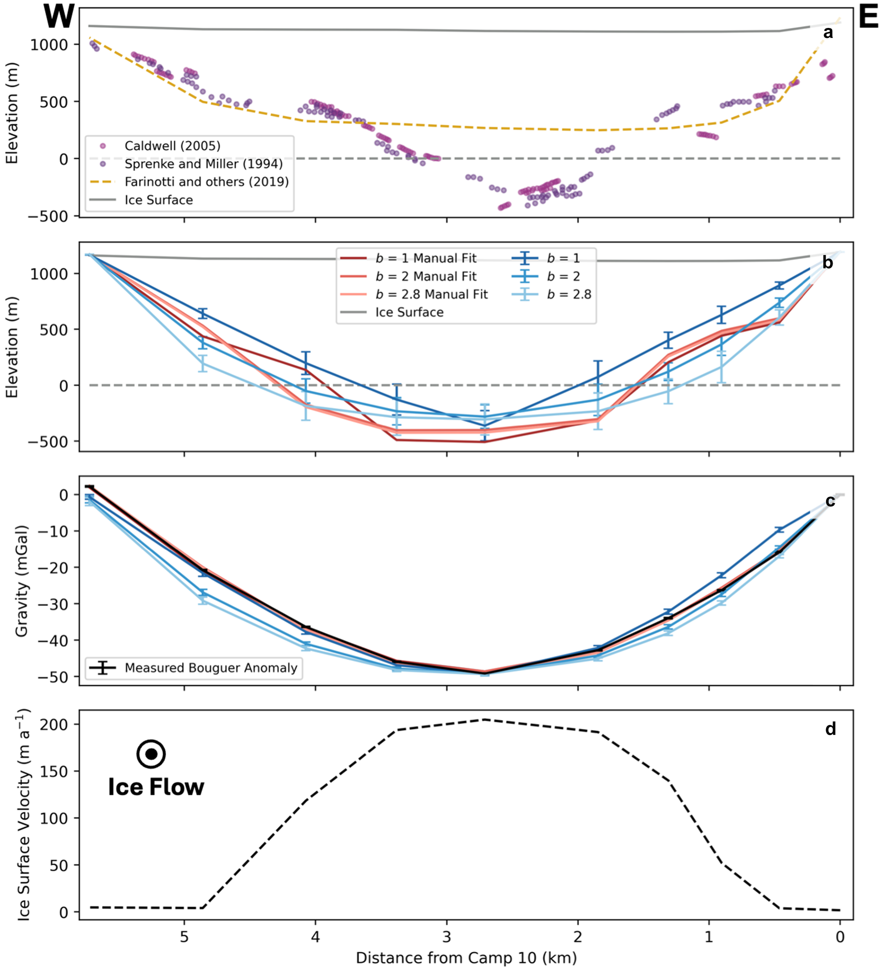
Results for Profile 4. (a) Results from previous studies. (b) Bed elevation results from this study. In blue colours are the results from the models with simple-shapes with b = 1 (V-shape), b = 2 (U-shape) and b = 2.8 (wide U-shape). In red colours are the manual-fitting results for each of these models respectively. (c) Gravity results from the models in (b). Legend as in (b). (d) Ice surface velocity extracted from NASA MEaSUREs ITS_LIVE project (Gardner and others, Reference Gardner, Fahnestock and Scambos2019).
Results for Profile 7a. (a) Bed elevation results. Legend for results from this study shown in (b). In blue colours are the results from the models with simple-shapes with b = 1 (V-shape), b = 2 (U-shape) and b = 2.8 (wide U-shape). In red colours are the manual-fitting results for each of these models respectively. (b) Gravity results from the models in (a). (c) Ice surface velocity extracted from NASA MEaSUREs ITS_LIVE project (Gardner and others, Reference Gardner, Fahnestock and Scambos2019).

Table of ice-thickness results
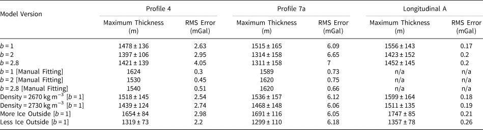
Maximum thickness refers to the point of maximum ice thickness on each profile and the associated uncertainty is the 95% confidence interval of the inversion results, as described in the text. Note that manual-fitting results do not have the associated uncertainty because they are not derived from an inversion. RMS error refers to the root mean squared error between the gravity anomaly of the model and the measured Bouguer anomaly.
Despite the models from each shape having different bed elevations, they all show a similar variation in the along-flow Longitudinal A profile. The deepest bed is at the downstream end of the profile with a gradual rise upstream, until a sharper rise in the elevation over two bedrock bumps at 2 and 7 km upstream of Profile 4. At the second of these bedrock bumps, the mean bed elevation rises above sea level in all models. The bed elevation then decreases again into the Matthes branch and moves below sea level for the V-shape model but remains around sea level for the U-shape and wide-U-shape models. These models provide end member solutions on the possible ice thickness distribution in the active model domain.
5.2 Manual fitting for across-glacier shape
The results from the across-flow profiles (Figs. 6 and 7) indicate that the glacier does not have a simple U- or V-shaped geometry. This can be seen in the misfit between the the measured Bouguer anomaly and the anomalies calculated from the simple-shape models that exceed the measurement uncertainties (blue lines) and the high RMS errors (Table 2). The misfit is more pronounced at Profile 7a where the simple-shape models all produce gravity anomalies that are too low on the West side and too high on the East side. These results suggest a glacier geometry that is both asymmetric and does not steadily deepen with distance from the glacier edge. These features can be seen in the glacier geometries derived from manual-fitting (red lines), which all exhibit broadly the same shape with an upper stepped section before a steeper slope leading into a flat and wide bottom. The asymmetry is again more pronounced at Profile 7a where the deepest portion lies to the eastern side of the glacier (Figs. 7; centre denoted by the deepest points in the simple-shape models). At Profile 4, the glacier appears more symmetric with the deepest portion lying mostly in the centre. There is also less consensus on the step feature on the west side of the Profile 4 model, with the only the V-shape model showing a step.
The manual-fitting models show much smaller variation in maximum ice thickness than the simple-shape models at Profile 7a with a total change among models of 31 m (Figs. 7). On the other hand, Profile 4 shows comparable variations with a total change of 94 m among models (Figs. 6). There are also some differences in the shapes among manual-fitting models. One such variation is on the western side of Profile 4 where the V-shape model produces a step-like features at around 4.5 km distance mark, whereas the U-shape and wide-U-shape models are deeper at this location and to compensate are then shallower than the V-shape model over distances 3.5 to 2 km. Similarly at 1.75 km distance across profile 7a, the V-shape model is deeper than the U-shape and wide U-shape models and then shallower at other locations to compensate. Some of these variations can be attributed to the shape outside the manual-fitting area (the same shape was tested across all versions and could not be fitted adequately) but some variations are likely due to the non-uniqueness inherent in gravity modelling and shapes with other variations could fit the data equally well. With these manual-fitting models, we significantly reduce the RMS error across Profiles 4 and 7a.
5.3 Sensitivity analysis
To assess the performance and assumptions made in our models, we conduct a sensitivity analysis. Here, we test the sensitivity of our results to the bedrock density and thickness of ice in the inactive model domain by running the inversion with the V-shape model. We compare them to the standard model with V-shape, hereafter called the baseline model.
5.3.1 Bedrock density
As we do not know the true bedrock density, we test the model with lower and higher background densities of 2670 kg m−3 and 2730 kg m−3. These runs result in increased ice thickness for the lower bedrock density and decreased ice thickness for the higher bedrock density (Figs. 8 and 9). These results are expected as the higher bedrock density leads to higher density contrast in the forward gravity-anomaly calculation, which means less ice is required to cause the same anomaly. However, this testing shows a relatively small variation within the range of densities tested. The variation in the mean maximum ice thickness across the density range tested is 79 m at Profile 4 and 68 m at Profile 7a, which are comparable with the uncertainty of the inversion results from the individual models.
Results of sensitivity analysis on Profile Longitudinal A. (a) Elevation of glacier bed, (b) gravity from models.

Results of sensitivity analysis at Profiles 4 and 7a. (a), (b) Bed elevation models from Profiles 4 (a) and 7a (b). (c), (d) Gravity model results from Profiles 4 (c) and 7a (d).

5.3.2 Ice thickness in the inactive model domain
We test the influence of different ice thicknesses in the inactive model domain by multiplying the ice thickness of Farinotti and others (Reference Farinotti2019) by 1.5 for the more ice scenario and by 0.5 for the less ice scenario. The results show that an increase in ice thickness in the inactive model domain results in an increase in ice thickness within the active model domain (Figs. 8 and 9). This is due to the measurements being relative to Camp 10, which is on the edge of the active model domain and therefore strongly affected by the changing ice thickness in the inactive model domain. The more ice scenario causes a more negative anomaly at Camp 10 and therefore a greater thickness of ice is required inside the active model domain to produce the same relative measured anomaly. The variation in maximum ice thickness at Profiles 4 and 7a is much larger for these scenarios than the density variation scenarios, showing the importance of including ice from the inactive model domain. Despite these larger variations in overall ice thickness, we still see the persistent features with the two bedrock bumps at 2 and 7 km upstream of Profile 4.
6. Discussion
6.1 Glacier geometry
6.1.1 Across flow
We derived an across-flow glacier geometry that has a similar shape at both Profiles 4 and 7a with a step-like feature and flat bottom, and is asymmetric at Profile 7a (Figs. 6 and 7). At Profile 4, we have some additional insight on the shape from the non-peer-reviewed seismic data. Both of the seismic results delineate a similar step feature, with flat sections at 0.75 km and 4.5 km from Camp 10, and the location of these is comparable to the gravity results from the manual-fitting results (Fig. 6). Such a step-like feature is also seen in the results of Nolan and others (Reference Nolan, Motkya, Echelmeyer and Trabant1995) at Goat Ridge, around 10 km downstream of Profile 4. The ice-surface velocity also gives some insight into the bed shape. The area of highest surface velocity across the profiles aligns with the area of deepest ice we have modelled with the manual fitting (at ~1.5−3.5 km on Fig. 6 and ~0.75−1.5 km on Fig 7). The velocity then gradually reduces through the step feature and drops to nearly 0 m a−1 towards the edges. The width of the area of velocity close to 0 m a−1 appears to align well with the end of the step-like feature, at 0.5 and 4.8 km across Profile 4 (Fig. 6) and 3 km across Profile 7a (Fig. 7). The additional evidence from the velocity and seismic data give weight to the step-like feature we modelled in the glacier geometry. On the other hand, the seismic data delineate a different shape for the deepest portion of the glacier than our results. Sprenke and Miller (Reference Sprenke and Miller1994) derived a relatively flat but narrow bottom and Caldwell (Reference Caldwell2005) find a more V-shaped bottom compared to our results that show a wide and flat bottom. These discrepancies could be due to difficulties in resolving narrow features with gravity data, error in the seismic-data analysis or indicating that the seismic measurements are delineating a layer of low-density sediment instead of the ice-bedrock contact. The surface-velocity data indicate a central fast-moving area similar in width to that of the flat-bottomed area we find but this is not a direct evidence of the width of the deepest portion of the glacier. As we do not have strong constraints on the geometry in the deepest portion of the glacier, some uncertainty remains on the maximum thickness. Therefore, although the manual-fitting shapes have maximum ice thickness closest to the V-shape model, we extend the range in which we expect the true maximum thickness to lie to be between the V- and U-shape models. We exclude the wide-U-shape from our range as it produces a result that is similar to the U-shape model but with a shape that diverges further from the manually derived geometry and has a higher RMS error across all profiles.
6.1.2 Along flow
As described above, the along-flow profile shows different ice thicknesses for different glacier-valley shapes (Fig. 5). However, there are bedrock rises at 2 and 7 km along the profile that persist across all model shapes, indicating their likely existence in the true bed profile. These bedrock rises occur at locations where tributaries are joining the main branch of the glacier. In the case of the rise at 2 km, there is a small tributary joining from the west with significantly lower ice-surface velocity than the main branch and a side basin to the east with very low surface velocity (Fig. 1). The rise at 7 km is where the Matthes branch converges with the main branch of the Taku. Previous modelling of longitudinal profiles of valley glaciers show that where a tributary joins the main branch, it is likely to be less deep than the main branch due to differences in the volume of ice discharge and hence capacity for erosion, creating a hanging valley (MacGregor and others, Reference MacGregor, Anderson, Anderson and Waddington2000; Anderson and others, Reference Anderson, Molnar and Kessler2006). This transition from hanging tributary to main branch is likely what is at the lee (downstream) side of the bedrock bump at 7 km where the Matthes joins the Taku. This lee-side slope is the most persistent feature in all of our inversion results, consistently being seen at the same location. Despite this, the length of the top of this bedrock bump and the magnitude of the elevation decrease on the stoss (upstream) side of the bump vary among models. The ice-surface velocity shows a decrease in velocity on the stoss side of the bump indicating there may be some compressional forces acting on the Matthes as it joins the main branch of the Taku. These compressional forces would lead to overdeepening as the ice works to maintain its flux of ice volume (Jiskoot and others, Reference Jiskoot, Fox and Van Wychen2017). The bedrock bump at 2 km along the profile is likely a result of the same combination of forces. Here, an overdeepening on the stoss side of the bump exists, likely due to the joining of the Matthes and the main branch of the Taku causing an increase in ice flux and the downstream slope is a step in the profile from the joining of the tributaries at 2 km (MacGregor and others, Reference MacGregor, Anderson, Anderson and Waddington2000; Anderson and others, Reference Anderson, Molnar and Kessler2006; Jiskoot and others, Reference Jiskoot, Fox and Van Wychen2017).
The locations of these bedrock bumps are also the two areas where the misfit in the gravity anomaly is relatively large. These areas of misfit can be seen at approximately 2.5 and 6 km upstream of Profile 4 (Fig. 5). As described above, these areas are close to where tributaries join and the misfits in these locations are likely due to our simplified models failing to capture the true variations in the ice thickness and glacier geometry. As we do not have data to further constrain the model in these areas, we do not attempt to improve the misfit here. The misfit locations indicate they are only showing a flaw in the modelling process where tributaries join the main branch, which is where we would expect the geometry to be more complex. There is a third area of misfit at 8.5 km upstream of Profile 4. There is no tributary joining here but there are some small side basins. The ice-surface velocity shows a sharp increase just before this misfit, indicating there is likely a structure in the subsurface which we are not capturing with our modelling approach. As before, we do not have the information to better resolve the feature causing the misfit at this location and it demonstrates the possible complexities in glacier-bed geometries.
6.2 Comparison with surface-inversion methods
The results from surface-inversion methods of Farinotti and others (Reference Farinotti2019) are the only other estimates of ice thickness across a larger area on the Taku. Comparing the bed elevation from Farinotti and others (Reference Farinotti2019) (yellow dashed line Figs. 6a and 7a) with the seismic results at Profile 4 and our gravity results at Profile 4 and 7a shows that the surface-inversion methods underestimate the ice thickness at the deepest, fastest moving portion of the glacier but their estimates are more comparable where ice is moving slower towards the edges of the glacier. The across-flow profiles show the surface-inversion methods also fail to capture the across-flow glacier geometry, instead delineating a very wide, flat bottom. On the along-flow profile (Fig. 5a) the surface-inversion methods show significantly shallower ice and also do not delineate the bedrock bumps that we model. They instead find one bedrock bump at ~8 km upstream of Profile 4 that is likely related to the change in ice-surface velocity there. The discrepancies in geometry and ice thickness from Farinotti and others (Reference Farinotti2019) shows the assumptions in the surface-inversions are likely not appropriate where the ice is flowing fast on the Taku (ice-surface velocities greater than ~15 m a−1). This in turn leads to not identifying features that could be important when modelling the Taku's future retreat.
The surface-inversion methods showing a more comparable results where ice flow is slow is important as our model relies on the assumption that the ice thickness results of Farinotti and others (Reference Farinotti2019) are a reasonable estimate in areas outside of our active model domain. The sensitivity analysis shows that a change in ice thickness outside the active model domain will cause a change in the same direction on the modelled ice thickness inside the active model domain. As described in section 5.1.2, this is due to the measurements being relative to Camp 10, which highlights the importance of correctly constraining the ice thickness in the side basins surrounding this location. In the basins surrounding Camp 10, the ice is flowing slowly, with maximum velocity of 11 m a−1, and hence we assume that at least at these locations the surface-inversion methods are providing a reasonable estimate of ice thickness. Additionally, the baseline model from the sensitivity analysis provides a result at Profile 4 that is more in line with the seismic results than either of the more- or less-ice scenarios, again indicating the surface-inversion methods give reasonable estimates outside of our active model domain. These variations close to Camp 10 additionally highlight the importance of obtaining more measurements close to the base station in a relative-gravity survey.
The discrepancies in the glacier geometry and ice thickness with the surface-inversion methods lead to different volumes of ice within the glacier, with implications for global sea level. To compare the potential ice volume among the models, we calculate the cross-sectional area at Profiles 4 and 7a for our results and those from Farinotti and others (Reference Farinotti2019) (Fig. 10). Here, we show the total area in the top bar and the area above sea level in the lower, lighter-coloured bar. The area above sea level is most important to compare as the volume of ice above sea level is what could contribute to global sea level. At Profile 4, the models we derived result in an increase in total area compared with Farinotti and others (Reference Farinotti2019) but most of this increase is below sea level. Conversely, the results at Profile 7a show an almost doubling in area across all our models and the majority of this increase is above sea level. These differences in cross-sectional area indicate there may be a substantially greater volume of ice above sea level contained in the Taku than previously estimated.
Cross sectional area of the glacier for each of the model runs. For each model labelled the top bar shows total area and the lower, lighter coloured bar shows area above sea level.

A similar trend of surface-inversion methods underestimating ice thickness compared to geophysical observations has been recorded at nearby Lemon Creek Glacier (Veitch and others, Reference Veitch2021) and in the Columbia River Basin in British Columbia, Canada (Pelto and others, Reference Pelto, Maussion, Menounos, Radić and Zeuner2020). Conversely, at Malaspina Glacier in Alaska, radio-echo sounding surveys revealed that Farinotti and others (Reference Farinotti2019) overestimated the ice thickness (Tober and others, Reference Tober2023). The authors suggest this overestimation may be due to the Malaspina being a surging glacier, causing varying velocities between years that are difficult to incorporate into surface-inversion methods (Tober and others, Reference Tober2023). These inconsistencies demonstrate the uncertainty associated with surface-inversion methods, as highlighted by Farinotti and others (Reference Farinotti2019) who note that their methods can produce local ice thicknesses that are up to twice as much as the observed values. Despite these local inconsistencies, the surface-inversion methods perform better when assessed against the mean ice thickness from all included measurements (Farinotti and others, Reference Farinotti2019). Nevertheless, these inconsistencies in ice thicknesses show the need to further improve inputs to surface-inversion methods and demonstrate that the bed topography from these methods is less reliable at individual glaciers.
6.3 Glacier-terminus evolution
We show the likely across-flow geometry of Taku Glacier at two locations and constrain the along-flow ice thickness within a reasonable range. Based on these results, we believe the along-flow ice thickness profile to lie between the V-shape and U-shape scenarios. This has implications for the future of the Taku, as it suggests the bed may lie below sea level into the Matthes branch of the glacier. We also delineate two bedrock bumps in our along-flow profile, features which have not been previously resolved on the Taku. Bedrock bumps such as these have also been suggested at other locations on the Taku. Nolan and others (Reference Nolan, Motkya, Echelmeyer and Trabant1995) discuss the need for a bedrock bump or another stabilising factor around the Bend profile (Fig. 1) to stop retreat in deep water during a ~200-year deglaciation period during the 19th century. Additionally, at Columbia Glacier and its former tributary Post Glacier, the retreating termini of both glaciers were found to stabilise at different times depending on when each glacier encountered a bedrock bump (Enderlin and others, Reference Enderlin, O'Neel, Bartholomaus and Joughin2018).
The terminus of the Taku is currently protected from oceanic forcing by a sediment shoal but if it retreats past this shoal, it could then potentially retreat rapidly. In this scenario, the bedrock bumps could play a vital role as pinning points during retreat in deep water, as has been shown for other glaciers. Bedrock bumps help stabilise the terminus of the glacier by reducing the water depth and therefore reducing the susceptibility to calving (Brown and others, Reference Brown, Meier and Post1982; Venteris, Reference Venteris1999), reducing buoyancy (Pfeffer, Reference Pfeffer2007; Post and others, Reference Post, O'Neel, Motyka and Streveler2011; Enderlin and others, Reference Enderlin, Howat and Vieli2013) and increasing the basal drag (O'Neel and others, Reference O'Neel, Pfeffer, Krimmel and Meier2005; Benn and others, Reference Benn, Warren and Mottram2007). While mass loss can still continue due to propagation of thinning upstream on the glacier (Mercer, Reference Mercer1961; Pfeffer, Reference Pfeffer2007; Post and others, Reference Post, O'Neel, Motyka and Streveler2011), these stabilisation points could temporarily slow the terminus retreat. They will additionally cause an episodic retreat with rapid retreat on a retrograde slope and slower retreat as the terminus moves up the prograde slope of a bump (e.g. Catania and others, Reference Catania2018; Frank and others, Reference Frank, Åkesson, De Fleurian, Morlighem and Nisancioglu2022). Our results indicate it is highly likely the bed is beneath sea level up to ~6 km upstream of Profile 4, corresponding to ~35 km upstream of the terminus, where the Matthes joins the main branch of the Taku. Further upstream, it is less clear if the bed is below sea level based on our results. Therefore, these pinning points could be important to help stabilise the terminus of the Taku during retreat in deep water.
7. Conclusion
We derived a 3D model for the bed elevation of a part of Taku Glacier using ground-based gravity measurements. From our measurements with supporting information from previous seismic measurements and surface-velocity data, we determine the across-flow geometry to have a wide, flat-bottomed centre and shallow step-like features closer the the sides. Based on this geometry and taking into account the uncertainties, we expect the along-flow maximum ice thickness to lie between that of a V-shaped- and U-shaped-valley scenarios. It is likely that the bed of the Taku is below sea level up to ~35 km upstream of its terminus, where the Matthes joins the main branch of the glacier. Upstream of this location, our modelling with associated uncertainty shows the bed is close to or below sea level. Despite the variation in models in the longitudinal profile, there are two bedrock bumps that are persistent across all the models. Such bedrock bumps could be vital in helping stabilise a retreat when the terminus of the Taku is in water and are likely to lead to an episodic, rather than steady, retreat. Additionally, we have found that surface-inversion methods underestimate ice thickness on the Taku and fail to resolve bed features that we have found, including the bedrock bumps and across-flow valley shape. These inconsistencies add to evidence that surface-inversion methods may not be suitable for accurately resolving bed topography of individual glaciers and indicate there is still uncertainty on the volume of ice contained in valley glaciers worldwide based on current estimates. We have highlighted some important factors when modelling glaciers with gravity data; the 2D assumption is not always valid and a 3D model with additional constraints may be more appropriate in some situations. Also, the contribution from anomalies outside the active model domain must be included in the gravity calculation and the area around a relative base station must be well constrained. Further work is required to reduce uncertainty on our results by, for example, increasing the number of gravity and seismic profiles across the glacier to better constrain the glacier shape. The need to interpolate between sparse constraints is a persistent issue in geoscience, especially in studies of the cryosphere. The novel method we present here maximises the value of the available constraints to improve bed-elevation estimates on Taku Glacier and could be applied to other under-constrained systems.
Data
Data and processing codes used in this study are available here: https://github.com/tul16152/Taku_gravity_2024.
Acknowledgements
We thank the Juneau Icefield Research Program for providing logistical support to carry out the fieldwork for this project as well as the many staff and students who helped collect the gravity and GNSS data. Special thanks to the student field team of Ellie Abrahams, Keeya Beausoleil, Galina Jonat, Sophia Ludtka and Jack Ryan and to field guides Isaac Gurdiel, Greg Kopache and Riley Wall. We also thank Seth Campbell for the loan of the GNSS receivers. We express gratitude to the Tlingit whose ancestral lands include Taku Glacier and the wider Juneau Icefield. We thank two anonymous reviewers and the scientific editor Shad O'Neel for their helpful comments, which improved the manuscript.


 Open access