


1 Introduction
The sea-ice structure is referred to as a mushy layer, due to its multiphase nature of entrapped liquid brine and solid ice (e.g. Feltham and others, Reference Feltham, Untersteiner, Wettlaufer and Worster2006; Middleton and others, Reference Middleton2022). Mushy layers develop due to the solidification of two-component solutions, resulting in an unstable solid–liquid interface and a solid porous structure filled with interstitial fluid (Wettlaufer and others, Reference Wettlaufer, Worster and Huppert1997). As the ambient temperature decreases, water freezes and sea ice grows, while brine within the interstitial spaces of the porous structure becomes more saline and denser than the underlying ocean (Wettlaufer and others, Reference Wettlaufer, Worster and Huppert1997). Since ice temperature typically increases towards the ice–ocean interface during ice growth, this results in unstable density profiles, with the dense saline brine flowing downwards through the mushy layer, across the ice–water interface and into the underlying water (Notz and Worster, Reference Notz and Worster2009). The dense brine is replaced with the less dense ocean water flowing upwards, resulting in buoyancy-driven convective flow within the mushy layer (Middleton and others, Reference Middleton, Thomas, De Wit and Tison2016; Notz and Worster, Reference Notz and Worster2009; Worster, Reference Worster1997). Worster (Reference Worster, Davis, Huppert, Müller and Worster1992, Reference Worster1997) describes two modes of convection that develop, namely mushy-layer and boundary-layer convective modes (hereafter referred as internal and interfacial convection, respectively). The former results in larger-scale convection, leading to the formation of long vertical vents, while the latter results in a smaller-scale loss of brine near the ice–water interface (Middleton and others, Reference Middleton, Thomas, De Wit and Tison2016; Worster, Reference Worster1997). The vertical vents, known as brine channels, act as conduits for the expulsion of the dense saline brine into the underlying water, further resulting in large-scale desalination of sea ice (Notz and Worster, Reference Notz and Worster2009; Wells and others, Reference Wells, Wettlaufer and Orszag2011). The fluxes associated with the salt- and freshwater floes during ice growth thus affect both the salt distribution and density of the underlying ocean and hence, the ocean overturning circulation, making it vital to investigate (Pellichero and others, Reference Pellichero, Sallée, Chapman and Downes2018). The water layer lying directly underneath the ice, which is further impacted by the ice, is known as the ice–ocean boundary layer (IOBL) (Keitzl, Reference Keitzl2015). Within the ocean, the IOBL is considered to consist of the sublayer and the mixed outer layer (Keitzl, Reference Keitzl2015; Mcphee, Reference Mcphee2008). Turbulence within the ocean resulting from shear forces and wave action lead to convective mass exchange in the mixed layer, while the sublayer is assumed to allow for diffusive exchanges due to the ‘no-slip’ condition that is described in fluid dynamics (Keitzl, Reference Keitzl2015; Keitzl and others, Reference Keitzl, Mellado and Notz2016). This results in many past and current numerical models incorporating a diffusive mass transfer model at the ice–water interface, which has an impact on one of the boundary conditions of the IOBL and estimated ice-melt rates.
The convective flow dynamics of the mushy layer has previously been numerically and experimentally investigated (Wettlaufer and others, Reference Wettlaufer, Worster and Huppert1997; Worster, Reference Worster1997; Wells, and others, Reference Wells, Wettlaufer and Orszag2011; Notz and Worster, Reference Notz and Worster2009; Worster and Wettlaufer, Reference Worster and Wettlaufer1997; Niedrauer and Martin, Reference Niedrauer and Martin1979). Wettlaufer and others (Reference Wettlaufer, Worster and Huppert1997) found that significant convection—and hence drainage of interstitial melt—only occurs after a significant mushy layer thickness has been reached and is hence linked to a critical Rayleigh number. The Rayleigh number is a dimensionless number that compares buoyancy forces to viscous dissipative forces within the porous mushy layer (Worster, Reference Worster, Davis, Huppert, Müller and Worster1992, Reference Wettlaufer, Worster and Huppert1997). In terms of fieldwork approaches, Notz and others (Reference Notz, Wettlaufer and Worster2005) investigated the temperature and impedance of sea ice in situ and determined there to be little to no salt loss via salt segregation from the interface, possibly due to the dilution from the underlying ocean water or to the limited resolution of the measurements. Further studies have been conducted in quasi-2D Hele-Shaw cells (two Perspex or glass sheets separated by a thin gap) to study the mushy layers formed from binary alloys (Chen, Reference Chen, Davis, Huppert, Müller and Worster1992; Peppin and others, Reference Peppin, Aussillous, Huppert and Worster2007; Peppin and others, Reference Peppin, Huppert and Worster2008; Schulze and Worster, Reference Schulze and Worster2005; Katz and Worster, Reference Katz and Worster2008; Middleton and others, Reference Middleton, Thomas, De Wit and Tison2016, Reference Middleton2022; Niedrauer and Martin, Reference Niedrauer and Martin1979). The use of a Hele-Shaw cell allows for the visualization of the brine channel features. Niedrauer and Martin (Reference Niedrauer and Martin1979) used a quasi-2D system and dye injections to investigate the formation and behaviour of brine channels. They suggested that the cold dense desalinating brine being expelled from the channel is replaced by warmer, less dense upward flowing water, further allowing for the freezing and melting of the brine channel sides allowing the channel to meander. This meandering behaviour can similarly be seen in work by Middleton and others (Reference Middleton, Thomas, De Wit and Tison2016, Reference Middleton2022). In contrast with the only fieldwork publication (Notz and others, Reference Notz, Wettlaufer and Worster2005), Middleton and others (Reference Middleton, Thomas, De Wit and Tison2016, Reference Middleton2022) demonstrated in their experiments that interfacial convection was occurring and contributed significantly to sea-ice desalination processes.
Different optical techniques have been employed to obtain images from artificial sea-ice growth in a Hele-Shaw cell. Middleton and others (Reference Middleton, Thomas, De Wit and Tison2016) performed traditional, adapted and synthetic Schlieren experiments (Settles, Reference Settles2001) to explore the brine expulsion of sea ice in a quasi-2D Hele-Shaw cell. Schlieren optics refers to capturing the density differences between transparent fluids due to their difference in refractive index (Settles, Reference Settles2001). The complexity of the Schlieren set-up allows for an optical image to be produced, as opposed to shadowgraphy which only produces a shadow of the object (Settles, Reference Settles2001). The former displays the first spatial derivative of the refractive index, which allows it to detect faint disturbances, while the latter detects the second spatial derivative, leading to a better view of more turbulent flows (Settles, Reference Settles2001). Middleton and others (Reference Middleton, Thomas, De Wit and Tison2016) performed a series of Schlieren experiments by capturing the refractive index differences between two parabolic mirrors resulting from density changes due to saline brine expulsion within the Hele-Shaw cell. Traditional Schlieren involved using the standard Schlieren set-up (shown in detail in Section 2.1). Adapted traditional Schlieren involved employing the traditional Schlieren optics but incorporating an additional light source to illuminate the ice layer from behind. Synthetic Schlieren involved a simpler set-up in comparison to the traditional Schlieren, using a random patterned background and image subtraction to highlight the convective and density changes. Although the traditional Schlieren is more complicated to implement, it exhibited a higher resolution of the brine expulsions into the underlying water when compared to the synthetic Schlieren and was thus used in this study (Middleton and others, Reference Middleton, Thomas, De Wit and Tison2016). In addition, direct light experiments allow the visualization of the brine channel formation and behaviour within the ice layer. Middleton and others (Reference Middleton2022) further improved on the experimental set-up by superimposing the direct light optical set-up with the Schlieren to allow for the ice and water view to be overlayed on the same field of view (FOV).
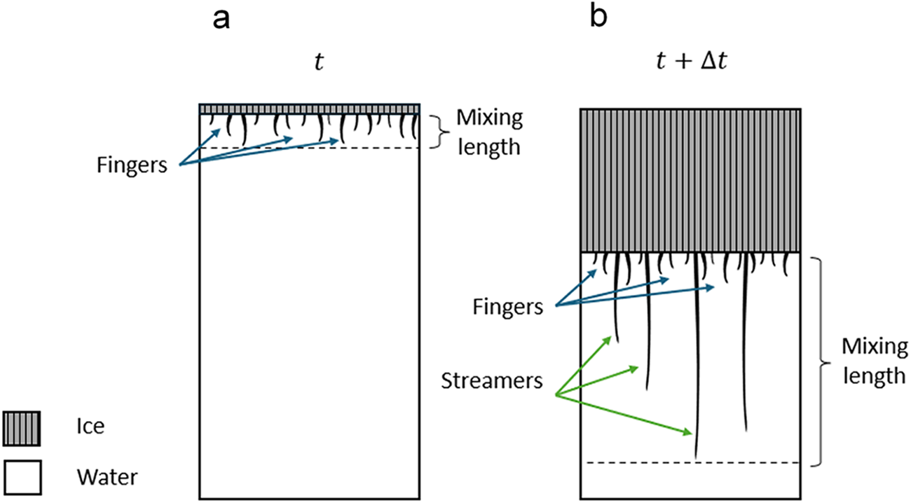
From the Schlieren experiments, Middleton and others (Reference Middleton2022) isolated the shorter and longer brine expulsions to determine their respective speeds at the onset of descent, and they were further able to determine the relative mass flux between the shorter and longer brine expulsions—known as fingers and streamers, respectively (see Fig. 1). The finger expulsions were not related to brine channels, and they were thought to result from interfacial convection due to salt rejection from the interface, i.e. via salt segregation. The streamer expulsions were instead the result of internally driven convection emanating from the brine channels within the mushy layer. It was also determined that smaller finger expulsions had a lower luminosity and only extended ∼1–2 cm below the interface, compared to the longer streamer expulsions which had a higher luminosity and extended much farther. The mixing length of the system is defined by the maximum extent from the interface and denotes the area within the water in which mass transfer occurs (Fig. 1). Since the quasi-2D system has no induced turbulence, the mixing length can be representative of the sublayer. The mixing length varies, depending on the time evolution of sea-ice growth. We currently do not know whether this variability is linked to temperature or ice thickness, since we lack high-resolution measurements near the interface. It was noted that the streamers exhibit an ‘on/off’ behaviour, whereby they do not continuously reject brines. Middleton and others (Reference Middleton2022) also observed that the relative mass flux of fingers contributed to significant amounts of desalination (∼30%), which is different from field observations made by Notz and others (Reference Notz, Wettlaufer and Worster2005) who observed that smaller-scale salt segregation resulting from finger expulsions are negligible. Thus, further investigation into internal and interfacial convection is necessary to elucidate the magnitude of this process
A schematic of brine expulsions emanating from ice in a quasi-2D system. (a) Approximately 15 min into the experiment, with fingers dominating the type of expulsions (see blue arrows). (b) After a certain time,  $\Delta t$, the ice grows thicker, and both streamers and fingers are expelled (see green arrows). The mixing length is denoted by the dashed line.
Middleton and others (Reference Middleton, Thomas, De Wit and Tison2016) provided a detailed description and view of the streamer and finger behaviours by performing basic digital image processing (DIP) via image subtraction to highlight the fingers and streamers. Middleton and others (Reference Middleton2022) further expanded on the previous processing, by including additional DIP steps by segmenting the expulsions to investigate the convective dynamics, performing image division and binarization. In this work, we demonstrate how more advanced image processing can be applied to better segment the areas of interest to allow for autonomous and continuous quantitative data collection from the qualitative videos. The two major shortcomings of the work conducted by Middleton and others (Reference Middleton2022) involve the limited selection of timescales for data analysis and the manual calculation of the expulsion behaviour, descent velocity and hence the relative mass flux. Furthermore, only three experiments were performed to investigate the behaviour between fingers and streamers. This introduces a limited opportunity to study the dynamic behaviour within the system. Obtaining a higher frequency of data during additional experiments is required to strengthen conclusions drawn between internal and interfacial convection. We thus ran new artificial ice experiments in a quasi-2D Hele-Shaw cell to develop improved DIP techniques focusing on the water layer during sea-ice growth. The development of autonomous DIP algorithms is vital to obtain a high-frequency time series, which would display the behaviour of internal and interfacial convection over the whole experimental period and eliminate the potential biases involved in manual selection of limited snapshots for analysis. The aim is to provide a better understanding and continuous quantification of the salt segregation and gravity drainage desalination mechanisms by investigating the expulsion of streamers and fingers. Currently, there are limited experimental studies investigating the desalination of sea ice (Middleton and others, Reference Middleton, Thomas, De Wit and Tison2016, Reference Middleton2022; Notz and others, Reference Notz, Wettlaufer and Worster2005). Of these studies, Notz and others (Reference Notz, Wettlaufer and Worster2005) investigate sea ice on a scale too large to obtain measurements close to the interface, i.e. in the sublayer. Middleton and others (Reference Middleton, Thomas, De Wit and Tison2016, Reference Middleton2022) proposed a method to visualize this layer but lacked the processing tools to strengthen their conclusions. This study uses the experimental method shown by Middleton and others (Reference Middleton, Thomas, De Wit and Tison2016, Reference Middleton2022) enhanced with a novel image processing method to obtain higher-resolution, continuous monitoring and improved temporal evolution of gravity drainage and salt segregation. In addition to advancing on the monitoring of the aforementioned types of desalination, we also visually demonstrate the extent and behaviour of the sublayer by showing that the sublayer is indeed turbulent, even in the absence of externally induced turbulence. Furthermore, we show that using this method allows for the statistical analysis of the convective features, which was not previously achievable. These discoveries are pivotal, since they contradict previous accepted norms on desalination and the sublayer, thereby making them vital to incorporate into current parameterizations and numerical models moving forward.
2. Methods
2.1. Experimental set-up
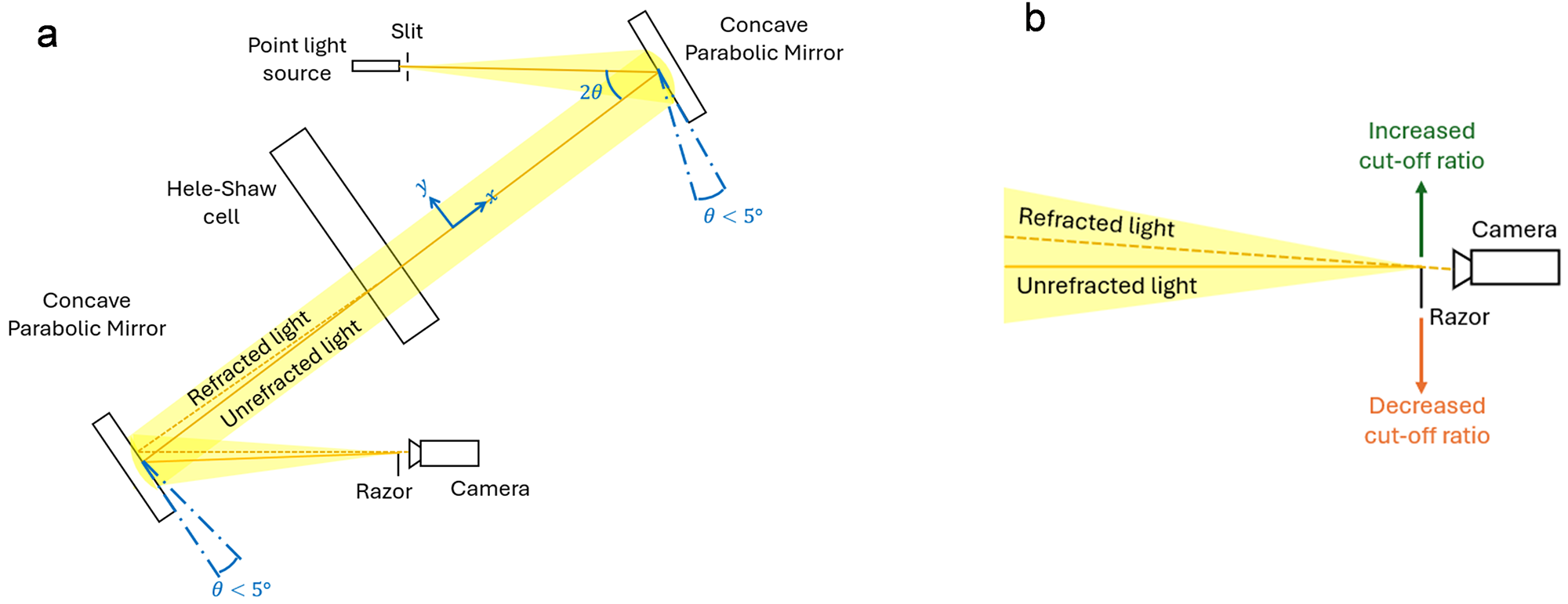
Experiments were conducted using a quasi-2D Hele-Shaw cell (604 mm × 348 mm × 3 mm) that was mounted in the same set-up described by Middleton and others (Reference Middleton2022) within a temperature-controlled laboratory. The cell was filled with a 35 ppt aqueous sodium chloride (NaCl) solution and placed within view of a GT2000C Prosilica camera. A lid with an inflowing chilled alcohol solution was used to apply a forcing temperature of −20°C to the top of the cell. The laboratory was maintained at a temperature of −0.5°C, since a lower temperature would be too close to the freezing point of the solution and result in dendritic ice growth and a non-uniform interface. Working in a closed system has shortcomings with respect to the underlying salinity, which increases as the experiment progresses, as opposed having a constant ocean salinity. Although working within a quasi-2D system might hamper the 3D formation of brine channels which would impact desalination, Middleton and others (Reference Middleton, Thomas, De Wit and Tison2016) state that the main brine channel collector should not be impacted. They further believe that the mass balance of the incoming and outgoing brine should remain consistent. A schematic of the Traditional Schlieren optical set-up is displayed in Figure 2a. To avoid the consequence of having optical aberrations negatively impacting the obtained Schlieren image, the angle between the mirrors and optical axis ( $\theta $) is both minimized ( $\theta \lt 5^\circ $) and placed at equal angles to each other (Settles, Reference Settles2001).
(a) Schematic showing the Schlieren laboratory set-up. The light path is highlighted, and both the refracted and unrefracted paths are indicated by the solid and dashed lines respectively. The angle between the central optical axis and the mirrors is kept below 5° and the angle between the light source and the mirror is double the angle of the mirror. The experimental system was set up in accordance with the system outlined in Settles (Reference Settles2001). (b) Detailed view of the placement of the razor in the current set-up (vertically placed) and the effect of increasing or decreasing the cut-off ratio, which results in less or more light being captured by the camera.
The cell, filled with the NaCl solution, was placed in the temperature-controlled laboratory for 8 h, to allow both the solution temperature and cell temperature to be constant before the start of the experiment. The cooling was then switched on to allow unidirectional cooling via the lid from the top. Timelapse images were obtained every 10 s, and a shutter time of 3800 s was used to capture the growing ice over a period of 15 h. Three experiments were performed at these conditions to visualize the dynamic behaviour of the brine expulsions, the resulting images of experiment three are seen in video 1.
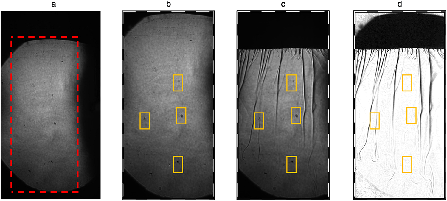
A knife-edge is required to capture transparent objects using Schlieren optics (Settles, Reference Settles2001). The knife-edge should be positioned at the focal point of the light and is used to block the unrefracted light from passing, thus only allowing the refracted light resulting from density changes within the cell to pass and be captured by the camera. The visualization of the Schlieren effect is dependent on the placement and type of knife-edge (Settles, Reference Settles2001). An increase in the cut-off ratio, i.e. allowing less light to pass (Fig. 2b), increases the sensitivity to visualize the Schlieren effect; however, it simultaneously decreases the FOV by introducing shadows around the sides of the image (see green boxes in Fig. 4a).
2.2. DIP approach
The quantitative data of interest involve the temporal evolution of the number of expulsion rejections and the average length of the expulsions to determine the relative mass flux contribution of fingers and streamers, and hence the contribution of salt segregation to desalination. Another variable of interest is the mixing length, which is defined by Middleton and others (Reference Middleton2022) as the maximum descent of expulsions from the interface. Due to the high-frequency dataset that is obtained from the timelapse images, this definition can be further explored to give insight on the changes in the diffusive sublayer below the ice–water interface using DIP methods.
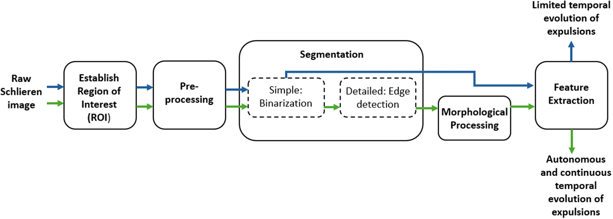
Since the use of Schlieren optics allows phase differences within transparent media to be seen as colour or (depth) changes, the expelled brine of higher density can be visualized due to its difference in pixel intensity compared to the surrounding water. The pixels within the image can further be manipulated via spatial processing to obtain desired information. Two types of spatial processing are used, namely intensity transformations and spatial filtering. While intensity transformations involve pixel manipulations of a digital image based on a single pixel intensity, spatial filtering of digital images involves altering an image by recalculating the value of each individual pixel within an image based on the central pixel and its neighbouring pixels using spatial kernels (Gonzalez and Woods, Reference Gonzalez and Woods2018). A spatial kernel is a matrix of specific size and with specific coefficients, which determines the size of the neighbourhood and type of operation. More details on the types and sizes of kernels are discussed in Section 3.2.1. Multistage algorithms used to segment objects within images do exist; however, it is difficult to adjust the algorithm to specifically detect the streamers and fingers. The best approach was thus to develop a DIP algorithm specifically to detect, isolate and obtain data from the expulsions seen in the Schlieren images. The approach to develop the DIP algorithm was followed by the steps outlined by Gonzalez and Woods (Reference Gonzalez and Woods2018). An overview of the approach can be seen in Figure 3 and is further outlined below.
Overview of digital image processing steps used in the proposed algorithm adapted from Gonzalez and Woods (Reference Gonzalez and Woods2018). The blue arrows indicate the approach used by Middleton and others (Reference Middleton2022) and the green arrows indicate the approach used in this study.
Establishing an exploitable region of interest (ROI) is important since this will be the region in which we obtain the data for further processing. The sensitivity of the Schlieren system to highlight density changes relies on the cut-off ratio, controlled by the position of the razor blade (Section 2.1). Increasing the cut-off ratio leads to increased sensitivity to density changes, thereby allowing a better-defined view of the brine expulsions. There is a trade-off between the cut-off ratio and FOV, whereby we need to maximize both the FOV and the brine expulsion definition prior to processing.
Preprocessing steps are applied to the cropped image to reduce the noise and filter out any artefacts that may interfere with data acquisition. We aim to remove as much of the inhomogeneity and background artefacts in the raw image as possible. Since the artefacts and background inhomogeneity remained consistent for the duration of the experiments, the images were normalized based on a reference image taken before the experimental run began. An elementwise pixel-by-pixel division of subsequent images with the reference image was performed to correct the background colour and remove the artefacts.
Once the image is normalized, a two-step segmentation process is applied. Firstly, a binary threshold is used to segment the expulsions so they consist of a singular pixel colour of white, while the background consists of a singular pixel colour of black. To obtain the correct threshold value to maximize the data obtained and minimize the noise, a threshold test is performed for each experimental run. An optimal threshold is required to differentiate between what is classified as ‘noise’ and what is classified as usable data. Applying this simple form of segmentation helps to refine the output from subsequent algorithms. There are two regions of interest—namely, the ice–water interface and the expulsions. To successfully isolate the interface, a smoothing filter is employed to decrease the appearance of expulsions.
More detailed segmentation processes are further explored to refine the output from the simple segmentation. These processes include boundary extraction methods and edge-detection methods based on detecting local discontinuity in the intensity at the boundary of an object using neighbourhood pixels (Gonzalez and Woods, Reference Gonzalez and Woods2018; Shrivakshan and Chandrasekar, Reference Shrivakshan and Chandrasekar2012). The main difference between these two techniques is that the former is based on a single pixel intensity while the latter is based on the neighbourhood of pixels surrounding the individual central pixel. Edge-detection based methods can further be separated into gradient-based and Laplacian-based operators, where the former uses operators to estimate the maximum and minimum in the first-order derivative, while the latter searches for the zero-crossings of the second-order derivative (Gonzalez and Woods, Reference Gonzalez and Woods2018; Maini and Aggarwal, Reference Main and Aggarwal2009; Shrivakshan and Chandrasekar, Reference Shrivakshan and Chandrasekar2012). The first-order derivative provides information on the occurrence of an edge, while the sign of the second-order derivative provides information on which side of the edge the pixel lies (Gonzalez and Woods, Reference Gonzalez and Woods2018). Since we only need to identify the edge, the first-order derivative is computed, applied and explored to visually determine which application is best for the algorithm. The result of the segmentation is seen in video 2.
After the object boundaries are defined, it is necessary to classify the image into areas of interest and non-interest by assigning pixels to either the foreground (white) or background (black) in the image. This can be achieved using morphological features, such as intersections and unions, that use mathematical set theory as a basis (Gonzalez and Woods, Reference Gonzalez and Woods2018; Soille, Reference Soille1999). Connected component labelling is a tool used to classify pixels of segmented objects as foreground pixels belonging to the object set based on a neighbourhood connectivity, while classifying pixels outside of the object set as background pixels (Gonzalez and Woods, Reference Gonzalez and Woods2018). A connected set is defined as all pixels of an object that can be joined by a path of pixels of the same object, with the path being dependent on the neighbourhood connectivity (Soille, Reference Soille1999). Assume we have a foreground object A consisting of pixels X, and background B consisting of pixels Y. The process to determine the connected set involves iterating throughout the image (I) and producing a new image, I1, consisting of the pixels corresponding to object A (X pixels) and neglecting the background (Y pixels). We start with I1 until Ik-1, where k equals the number of objects within the image and N refers to the chosen neighbourhood pixel connectivity (see eq. (1) (Gonzalez and Woods, Reference Gonzalez and Woods2018)). The final video after the application of the connected component labelling is seen in video 3.
 \begin{equation}{I_k} = \left( {{I_{k - 1}} \oplus N} \right) {\cap\ I\ k = 1, 2, 3,} \ldots \end{equation}
Lastly, feature extraction and description involve detecting, extracting and describing meaningful information from the streamers and fingers obtained resulting from the preceding DIP steps and representing it quantitatively. Since fingers are shorter in length than streamers, the separation of these features is based on the length, with fingers found being 20 mm and below. The justification of this choice is further discussed in Section 3.3.1. Due to the Schlieren optical set-up, we do not yet have an image with features sensitive enough to separate the expulsions based on luminosity.
3. Results
3.1. Raw images
Examples of raw images obtained from the Schlieren experiments are shown in Figure 4 and the full video containing these images is shown in video 1. The separation in the figures marks the significant timestamps chosen to see a change in system dynamics, 11–40 min (initial and less defined expulsions progressing to a larger number of well-defined streamers) and 4–15 h (decrease in number of streamers and change in expulsion behaviour). Fingers and streamers differ both in their lengths, and their refractive indices. Fingers exhibit shorter lengths and less definition (seem ‘shallower’) (compare Fig. 4b to Fig. 4d). The onset of finger expulsions begins at an average of 11 min into the beginning of each experiment. Within the first 20 min of the experiment (Fig. 4a–c), the expulsions seem to be less defined and lighter in colour when compared to expulsions later in the experiment (see Fig. 4d). Throughout the experiments, we can see that streamers and fingers are expelled from the interface and are seen to meander across the cell. Streamers are typically longer in length, compared to fingers and they exhibit a stronger Schlieren effect (they are less ‘flat’). The streamers seem to be the most active (greater in number) after 40 min (see Fig. 4d) into the experiment. Thereafter, the expulsions become lower in number, with fewer streamers being visible (see Fig. 4e). Although the streamers are seen to decrease in both length and number, the fingers remain active from the beginning of the experiment (Fig. 4a) until its end (Fig. 4h).
Time series images of the raw Schlieren optical experiments. The room temperature was set to −0.5°C and the applied forcing temperature at the top of the cell was −20°C. (a) The darker shadow areas highlighted by the green boxes are a result of the Schlieren cut-off ratio. The ice is denoted by the black area and the water is denoted by the grey area. (b) There are only shorter interfacial fingers present (see white arrows) (c) and (d) Longer streamers begin to form (see orange arrows) and a total of 13 streamers are present after 41 min. The blue arrow shows the advancing ice–water interface. The finger expulsions remain near the interface and are present even before the onset of streamers. Before 19 min, it seems that the most activity is attributed to finger expulsions. The alternating black and white border represents a scale of one cm and thus the entire FOV is 19 cm × 10 cm. (e) The 13 streamers reduced to 6 when approaching 4 h. Fingers are seen to slant towards the right (see red arrow). (f) Fingers and two streamers are flowing towards the right. The middle streamer can be seen to influence the last streamers flow direction. (g) The fingers stop flowing to the right and exhibit a straight downward descent. Likewise, the streamers follow a similar flow direction. (h) End of the experiment showing six fingers and one streamer.
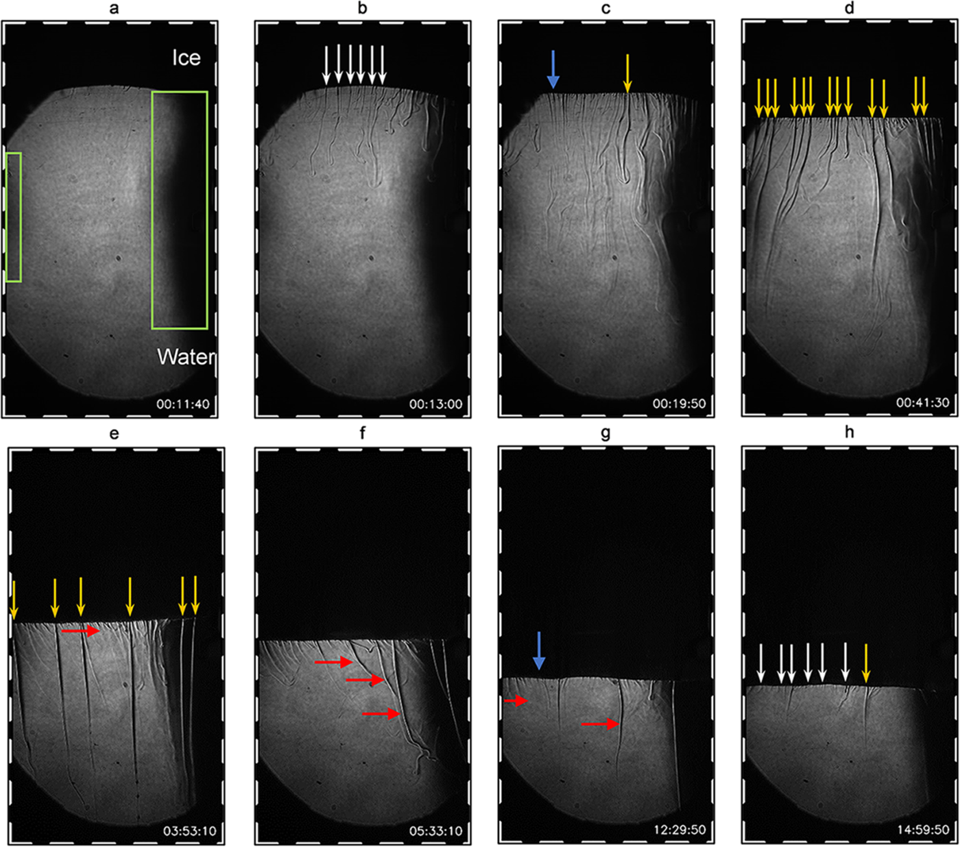
The expulsions found later exhibit a smaller Schlieren effect and do not penetrate as deep as the expulsions earlier in the experiment, leading to the interpretation that the density—and hence salinity—of the streamers eventually decreases and perhaps brine channels desalination slows down after a period of time (roughly 7 h).
The refractive index of fluids is temperature, pressure and concentration dependent, with various studies using methods to investigate these dependences (Austin and Halikas, Reference Austin and Halikas1976; Bremer and others, Reference Bremer2017). Since we have no quantitative measurements of salinity and temperature, we cannot yet determine which phenomenon has a greater influence on the refractive index. However, we do know that the internal and interfacial convection that takes place during solidification involves compositional and thermal gradients (Worster, Reference Worster1997; Wettlaufer and others, Reference Wettlaufer, Worster and Huppert1997). The former impacts internal convection, linked to gravity drainage (streamers) while the latter impacts interfacial convection, linked to salt segregation (fingers) (Middleton and others, Reference Middleton, Thomas, De Wit and Tison2016). This suggests that streamers are compositionally driven via salinity changes with a larger refractive index difference (as seen by the more defined expulsions), while fingers are more thermally driven with a smaller refractive index difference (as seen by the less defined expulsions near the interface).
3.2. DIP of Schlieren images
3.2.1. Preprocessing
Before performing further processing, the ROI is established (Section 2.2) whereby the areas of non-interest—the darker shadows due to the cut-off ratio and the areas out of the camera FOV—are cropped according to the outline (Fig. 5a).
(a) Original raw image obtained from the Schlieren optical system with size 19 × 10 cm; the ROI is outlined in red, (b) the final cropped image used for further processing (10 × 7 cm), (c) cropped image at 83.3 min into the experiment, where we note inhomogeneous background shading and (d) resultant image after preprocessing and shading removal. The orange boxes show the image artefacts that are removed after preprocessing
The background of the image can be seen to be inhomogeneous in terms of pixel intensity, where there are areas of lighter and darker grey. Additionally, there are circular and irregular shaped specks within the image. Since these spots do not move and remain consistent across all of the frames within the videos, they are most likely due to the lens and equipment used during the experiments. The image is normalized, according to the method described in Section 2.2, to remove the background and equipment interferences. The cropped reference image, the cropped image at 83.3 min, and the subsequent preprocessed image at 83.3 min are displayed in Figure 5b–d.
3.2.2. Segmentation of the ice–water interface and expulsions
Two separate binary thresholds are performed (Section 2.2), firstly to isolate the ice–water interface to determine the ice thickness and growth rate over time (See in supplementary information Fig. S1c–e), and secondly to isolate the expulsions to investigate the streamer and finger behaviour (Fig. 6b–d). To isolate the ice–water interface, the image is further cropped to only focus on the ice and water later (the only remaining black area represents the ice layer). A smoothing filter is applied to prevent detection of the underlying expulsions. Thereafter, the image is segmented at various threshold values to test the sensitivity of the algorithm (Section 2.2). A threshold too low will underestimate the ice thickness and introduce interference at the top of the ice layer (Fig. S1c), while a threshold that is too high will overestimate the ice thickness (Fig. S1e). An appropriate threshold based on inspection is chosen (sigma = 60, Fig. S1d), which provides the most accurate segmentation of the ice layer.
(a) Preprocessed image. The orange boxes show the interference of the background if the sigma value is too low (b–d) Images showing a binary threshold of 140, 190 and 240, respectively, for segmentation of steamers and fingers. The orange boxes highlight breakages in the streamers, while the blue boxes show the less dense fluid interferences that become more pronounced as the binary threshold increases.
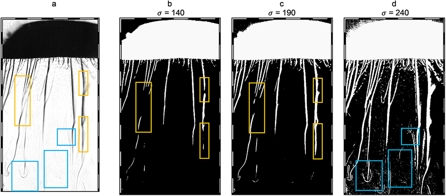
To optimally isolate the streamers and fingers, again different thresholds were investigated during the binary threshold. A lower threshold in Figure 6b shows either breaking in the expulsions or it highlights areas in which the refractive index difference between the streamers and underlying water is too small (orange boxes). Consequently, selecting a larger threshold (Fig. 6d) shows too much noise in the background (blue boxes). A threshold is thus chosen again based on inspection to highlight the Schlieren effect (i.e. the specific darker shadow and adjacent light area), but also to minimize noise. Increasing the threshold beyond this would result in the detection of residual disturbances in the water below, that have a minimal—if any—Schlieren effect (Fig. 6d). A trade-off thus needs to be made to determine a ‘high enough’ refractive index difference, before the noise interacts with the algorithm.
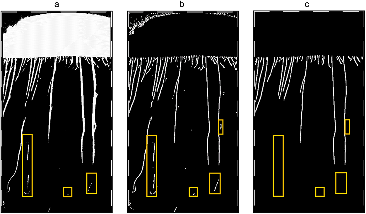
Contour detection and extraction were applied to the preprocessed and binary images from Figure 6 as a form of boundary extraction (Fig. S2 and Section 2.2). Since brine gets expelled from the interface and it is always in contact with the interface, the contour identifies the expulsions and the ice layer as a single entity (Fig. S2b). Thus, an additional step would be required to further separate the interface, fingers and streamers. This could be done through extraction and separation of their vertical lengths from the preceding contour, i.e. the line connecting all of the expulsions (Fig. S2b) are segmented into multiple smaller segments, allowing the expulsions to be separated and further fingers and streamers to be determined, based on their respective lengths (see Fig. S2c). However, as seen by comparing blue boxes in Figure S2b and c, the boundaries around the finger expulsions proved not well isolated, resulting in missing finger expulsions. An additional issue that contour detection and extraction pose is the discontinuity in the boundary of the streamers. The green box in Figure S2c shows breakages in the lengths of the streamers. It seems that sharp points (see blue arrows) along the length of the streamer—and even at the tip of the streamer—lead to breakages and thus issues in the calculation of lengths. Furthermore, boundary extraction itself leads to problems, since the total length of the contour surrounding the expulsions is measured, instead of only the vertical length of the expulsion from the interface.
A first-order differential edge detection approach was thus further pursued to segment the streamers and fingers, as described in Section 2.2. The Sobel operator in the x-direction was used to compute the changes in intensity using a convolution kernel size of 3, 5 and 7. An advantageous feature of the Sobel operator is that it allows for the isolation of features based on axes by computing the partial differential in the x- (horizontal) and y- (vertical) directions separately. This lets the vertical streamers to be detected, while neglecting the detections of the ‘sub-horizontal’ ice–water interface. Due to the fine detail of the finger expulsions, using smaller neighbourhood kernels resulted in discontinuities within the length of the fingers and streamers (see Fig. S3 in the supplementary information).
Kernel size of 3 resulted in a fragmented segmentation of expulsions with breakages in the lengths of fingers and streamers (see orange and red blocks in Fig. S3a–c). Kernel size of 5 resulted in a comparatively better image in terms of the expulsion length, with the fingers having fewer discontinuities (see Fig. S3b). The kernel size of 7 resulted in the fewest discontinuities of expulsions, especially when looking at the fingers. Since the refractive index difference of the fingers is smaller than that of the streamers, the segmentation of the fingers is more challenging than the segmentation of the streamers. Although using a kernel size of 7 does not eliminate all of the discontinuities, it does allow for the least breakages in the fingers and leads to more defined fingers and streamers that make it easier for the features to be extracted. It should be noted that although a larger kernel size does increase the thickness of the expulsions, during the calculation of relative mass flux, we use assumed average expulsion radii (0.5 mm for streamers and 0.35 mm for fingers, as determined by Middleton and others (Reference Middleton2022), to allow for consistency during comparison), thus the thickness determined by the kernel size would not impact subsequent results. This value was thus chosen in the algorithm.
3.2.3. Morphological processes: connected components analysis
The finger and streamer expulsions are not only vertical but are seen to slant diagonally over time (see Section 3.1). The expulsions from the ice–water interface are highly variable in terms of their movement and angle of expulsion, resulting from both the convective dynamics due to the density- and thermal-gradients within the underlying water and the meandering of the brine channels within the ice (Middleton and others, Reference Middleton, Thomas, De Wit and Tison2016, Reference Middleton2022). By applying the connected component analysis with an eight-neighborhood connectivity (Section 2.2), each expulsion is classified as its own individual object with its own index, making it easier to separate them based on physical characteristics such as length, width, starting and ending position. Although the preprocessing and segmentation algorithm was formulated to both maximize expulsion detection and minimize noise, it is difficult to achieve a perfect result. The algorithm was adapted to further decrease the noise by only extracting features emanating from the ice–water interface. The interface position over time is dependent on the sea-ice growth rate, which changes based on the initial conditions of the experiment. The developed algorithm accounts for this change in interface position over time, by firstly, segmenting the ice from the underlying water via segmentation and smoothing filters, as mentioned in Section 2.2. The position of this isolated interface was then tracked using a separate connected component analysis (Section 2.2 and video 3).
Although preprocessing and segmentation were performed to reduce noise and detect significant density changes, there are still significant amounts of smaller expulsions with small changes in luminosity, i.e. the lighter, less defined expulsions outlined in Figure 7b. Using the two connected component analyses, the smaller expulsions are removed, as seen in Figure 7c and video 2.
Complete steps of the DIP protocol. (a) Binary Schlieren image; (b) Application of the Sobel operator with kernel size of 7 and (c) connected component analysis with the set of restrictions showing the removal of additional noisy elements. The orange boxes highlight the removal on the noisy interferences in the contour image.
3.2.4. Streamer tracking
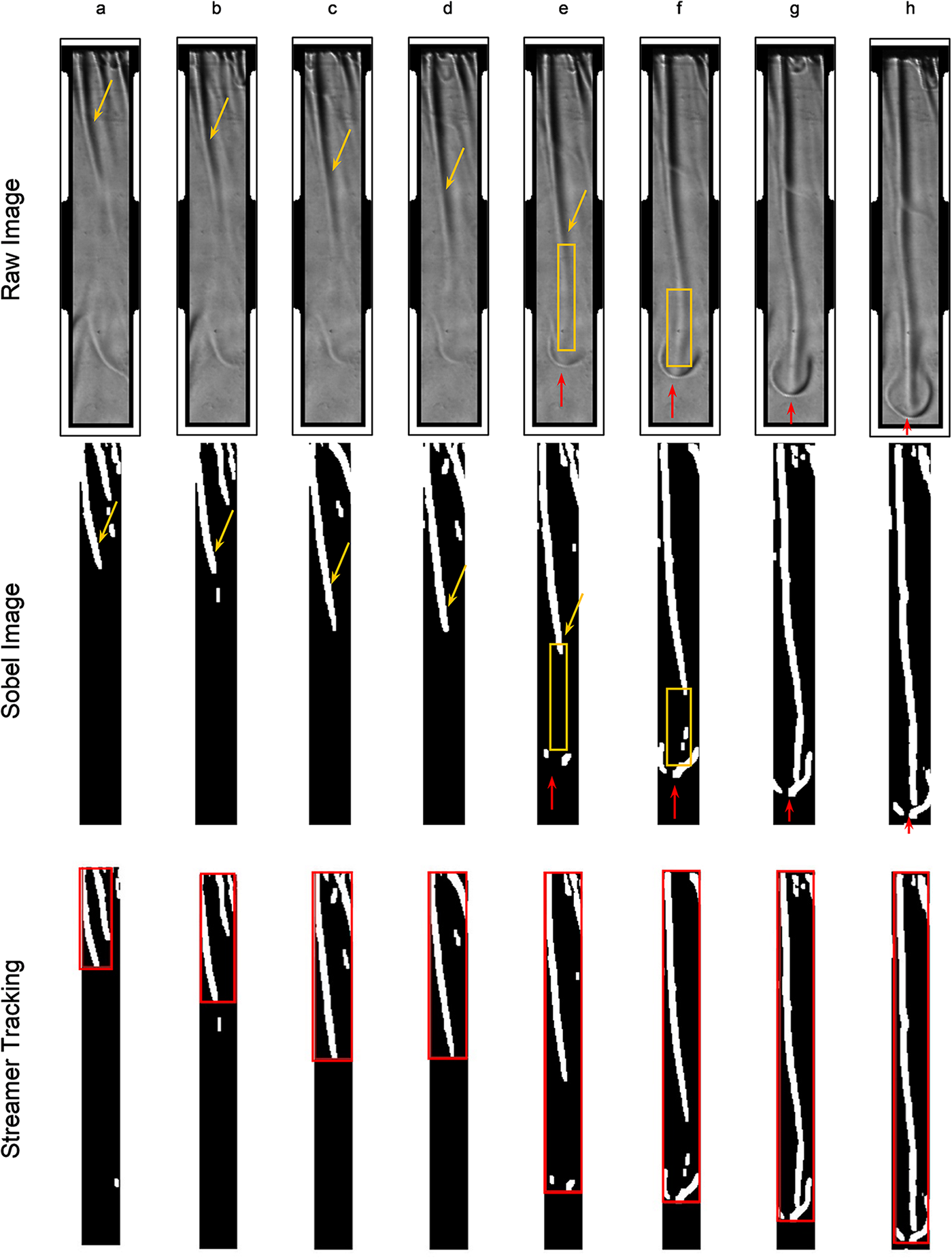
As described by Middleton and others (Reference Middleton2022), a limitation of using the Schlieren optical system is the inability to determine the steady-state velocity of the expulsions. Instead, only the descent speed of the expulsions can be determined and used to determine the relative mass-flux ratio of the fingers and streamers. The detection of the streamers is dependent on the luminosity of the expulsions; the larger the change in luminosity, the easier it will be to detect the streamer. There are instances where the luminosity change is small, which impacts the length detection. To improve the length determination, connected component analysis is used; however, new restrictions, based on the region centroid, are placed upon the areas of interest. Instead of separating the regions based on length, as was done to separate fingers and streamers, certain regions of interest were combined based on the distance between the region centroids—if this distance is close enough, it can be assumed that both regions belong to the same expulsion. Regions with centroids close together (in the x-axis, i.e. in the horizontal) were grouped together as a single streamer that was disjointed, due to the changes in the luminosity. This combined region is then tracked across frames to stitch the disjointed streamers together to allow for a more continuous length—and hence to improve the descent speed calculation.
Consider a single streamer as in Figure 8. Since the change in luminosity from the top of the streamer to the tip of rejection is not consistent, there are breakages in the streamer length (see Fig. 8e and f). By identifying the tip of rejection and linking the centroid of the tip to the streamer, the two areas can be virtually linked as a single expulsion, allowing for the stitching of the disjointed streamer and the tracking over a series of frames. It should be noted that the tracking and stitching of the streamers are autonomous, but the isolation of the streamers (i.e. locating a descending stream that exhibits the tip of rejection) are conducted manually. To achieve an autonomous method to identify the streamer with the specific set of conditions, additional machine learning algorithms will be required.
(a–d) Descent of a single streamer during Experiment 2. The streamer can be seen to steadily grow (see orange arrow) until the tip of rejection can be seen (see red arrow) (e–h). The orange boxes show the break in the stream length due to low changes in luminosity. The raw image of the streamer, the streamer after Sobel detection is applied and the result of the streamer tracking algorithm is seen. The red box shows the final stitched streamer. The alternating black and white border in the top row shows the scale that is spaced at 1 cm.
3.3. Feature extraction and quantitative data output
3.3.1. Sea-ice thickness and growth rate
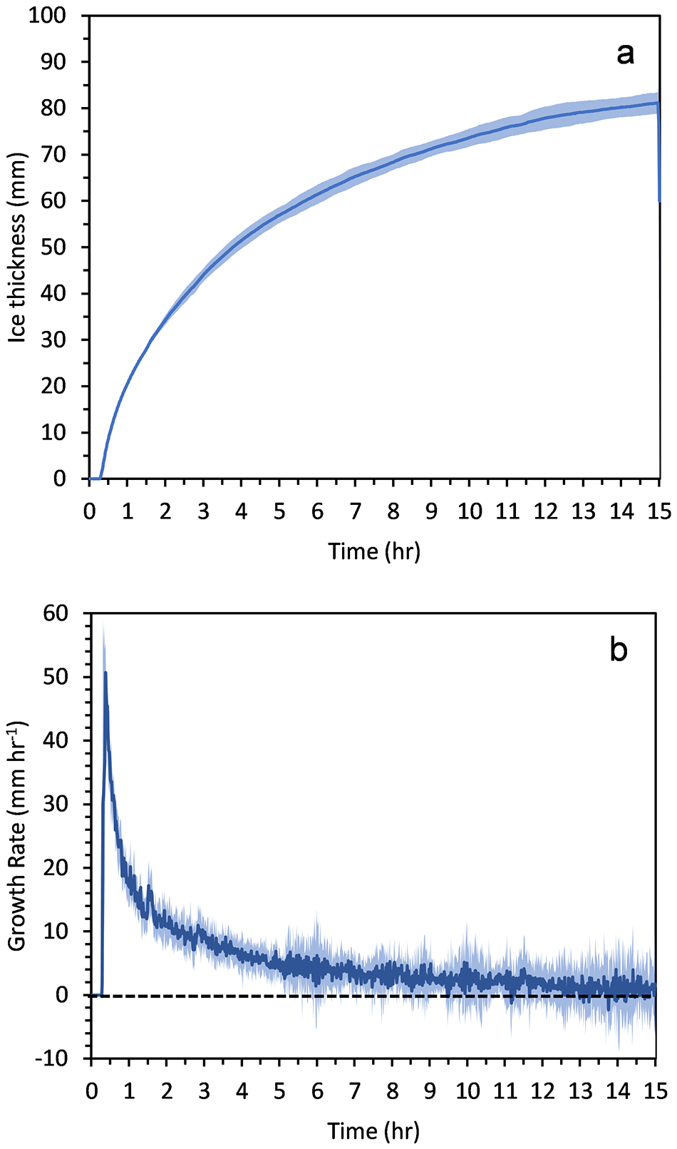
The sea-ice thickness (Fig. 9) over time for the three experimental runs were determined by isolating the ice layer and interface from the water layer. Over an experimental period of 15 h, we note an initial sharp increase in the thickness. This is exhibited across all three experiments and is consistent with ice thickness trends seen in Middleton and others (Reference Middleton, Thomas, De Wit and Tison2016, Reference Middleton2022). This initial sharp increase is attributed to a high thermal driving force at the beginning of the experiment and minimal insulation between the forcing temperature and the water layer. The growth rate was further calculated using the gradient method and is displayed in Figure 9b. Although there is a fluctuating trend in the growth rate, similar to Middleton and others (Reference Middleton, Thomas, De Wit and Tison2016), we note that there is an overall decrease in the local growth rate over time in all three experimental runs due to the increased insulation as the ice grows over time, thereby decreasing the conductive heat transport. The growth rate reaches minimum values after 5 h, with an average standard deviation of 3.72 mm h−1. The fluctuating growth rate could be a result of Mullins–Sekerka instability, which describes the formation of pertubations on the solid-liquid interface of supercooled multicomponent fluids (Anderson and others, Reference Anderson, Guba and Wells2022). The solid ice will grow and melt, due to the thermal and compositional changes; additionally, due to a build-up of pressure within the Hele-Shaw cell, the interface may become unstable resulting in fluctuating growth rates seen in Figure 9b (Anderson and others, Reference Anderson, Guba and Wells2022; Ben-Jacob and Garik, Reference Ben-Jacob and Garik1990).
Mean ice thickness (a) and ice growth rate (b) with time for three experiments. The shading represents the standard deviation, and the dashed line represents a growth rate of zero.
3.3.2. Internal and interfacial convection
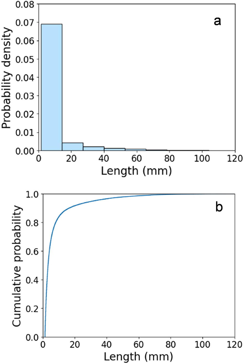
Once the expulsions have been segmented and classified as objects, they can further be separated based on length. Within the experiments conducted by Middleton and others (Reference Middleton2022), the first 10 mm below the interface shows the most activity in comparison to the first 30 mm, which was further attributed to the shorter finger expulsions’ contribution. To understand whether the length threshold for the fingers is limited between 10 and 30 mm, the probability density function (PDF) of Experiment 3 was plotted in Figure 10. Here, we see a skewed distribution with the probability of achieving a length below 20 mm being high (between 0.06 and 0.07), and in looking at the cumulative density function (CDF), we see that over 80% of values fall below 20 mm. Due to the high number of fingers, in comparison to streamers (as seen in Fig. 4), we can justify the choice of using 20 mm as a threshold to classify the separation of fingers and streamers. The PDF and CDF of all three experiments can be found in Fig. S4.
(a) Probability density histogram and (b) cumulative probability distribution for the lengths of the expulsions (fingers and streamers) in Experiment 3 during the 15-h experiment.
3.3.2.1. Number of fingers and streamers
The mean number of expulsions from the ice interface and the mean ice growth rate for the three experiments are plotted in Figure 11. Due to the high frequency of the data and to avoid the influence of noise, the number of rejections were averaged over a 60-s interval and these mean values were plotted. The number of fingers is seen to be significantly higher than the streamers and both sets of expulsions are seen to decrease over time, similar to the observations made by Middleton and others (Reference Middleton2022). There is also a higher variability in the number of finger expulsions in comparison to the streamer expulsions.
The mean number of rejections per minute for the fingers and streamers and growth rate of the ice for (a) over the 15-h experimental run and (b) over the first hour of the experimental run respectively obtained from the developed DIP algorithm. The dashed red line represents the panel examined in (b). The standard deviation across the three experiments can be seen as the shaded area surrounding each data set. The dashed black line represents a growth rate and number of rejections of zero.
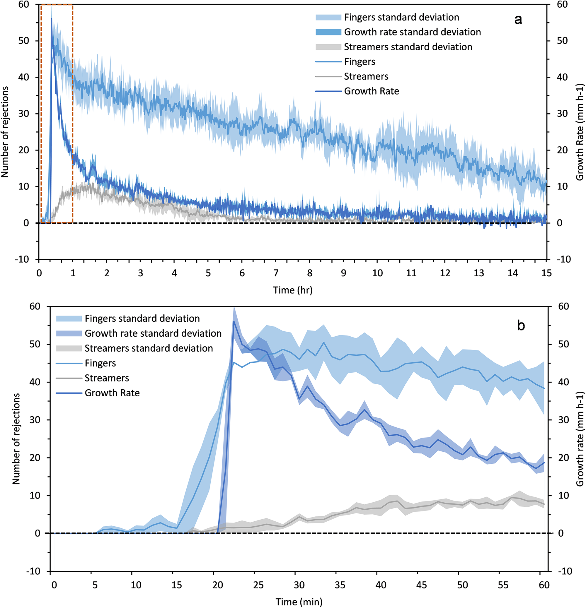
We see a low number of fingers that sharply increases over a short time-period (∼20 min to reach the maximum number of rejections) and fluctuates ∼40 rejections within the first 5 h. The total number of streamers increases at a slower rate (∼40 min to reach the maximum number of rejections) and fluctuates at ∼7 rejections within the first 5 h. During the first 15 min (see Fig. 11b), interfacial convection dominates and there are only fingers present (this is further seen in Fig. 4b and video 1). Thereafter, the streamers begin to be expelled, most likely due to the formation of brine channels and the onset of internal convection. The delay in the ice growth rate at the beginning (Fig. 11b) could be attributed to slight underestimations in the DIP step, resulting in the ice showing its presence after the finger expulsions. After 4–5 h, the number of streamers drop to near zero. After 5 h, the number of rejections has a 0.43 correlation with the ice growth rate, in comparison with a 0.27 correlation between 0 and 5 h. The absence of streamers at the beginning aligns with the understanding that a critical thickness must be reached to overcome viscous dissipative forces to allow desalination (Wettlaufer and others, Reference Wettlaufer, Worster and Huppert1997), and that the desalination depends on ice growth rates (Notz and Worster, Reference Notz and Worster2009). This trend is consistent with the observations made by Middleton and others (Reference Middleton, Thomas, De Wit and Tison2016, Reference Middleton2022), whereby the streamers exhibit an ‘on/off’ behaviour when the ice growth rate is at a minimum and relatively stable.
Although the streamers are significant in their length and in the amount of salt expelled when they are active, the large number of fingers have an impact on firstly, the direction of the streamer flow (Fig. 4e–g) and secondly, may have an impact on the amount of salt rejected, in the beginning of the experiment (when the streamers are not present) intermediately (after 5 h, when the streamers begin to exhibit their on/off behaviour) and at the end (when there is a significant decrease in the number of streamers). After 5 h when the ice growth rate is reaching its minimum values (0–15 mm h−1), the streamers are only active ∼54% of the time, which is a large reduction compared to the 92% of streamer activity within the first 5 h. This suggests that there could be a relationship between the ice growth rate and a slowdown in the expulsion of streamers. However, it should be noted that the closed system, such as the one in which we are working, results in an increase in salinity of the underlying water reservoir, further reducing Rayleigh numbers (due to a decreased density contrast between the streamers and the underlying water reservoir). This could result in potentially hampering the brine drainage through the streamers.
3.3.2.2. Average finger and streamer length
Using the developed DIP algorithm, the expulsions from the interface were isolated and were further segmented based on their length. The average length of the fingers and streamers of each experiment was determined and plotted (see Fig. 12). Similar to Section 3.3.2.1, the mean of the average length over a 60-s interval was plotted and the length threshold for segmenting fingers and streamers was chosen based on the Middleton and others (Reference Middleton2022) definition of 20 mm. The length can be seen to have many fluctuations over the 15-h period, with highest variance occurring in the first 5 h (Fig. 12). There is an increase in the average length at the beginning of the experiment until 1 h into the experiment. It should be noted that after 100 min, some of the streamers reach depths beyond the FOV and thus the results after this time will be slightly skewed. This observation is further seen visually in Figure 4e.
The mean average length of fingers and streamers over the 15-h experimental run obtained from the developed DIP algorithm. The standard deviation across the three experiments can be seen as the shaded area surrounding each data set.
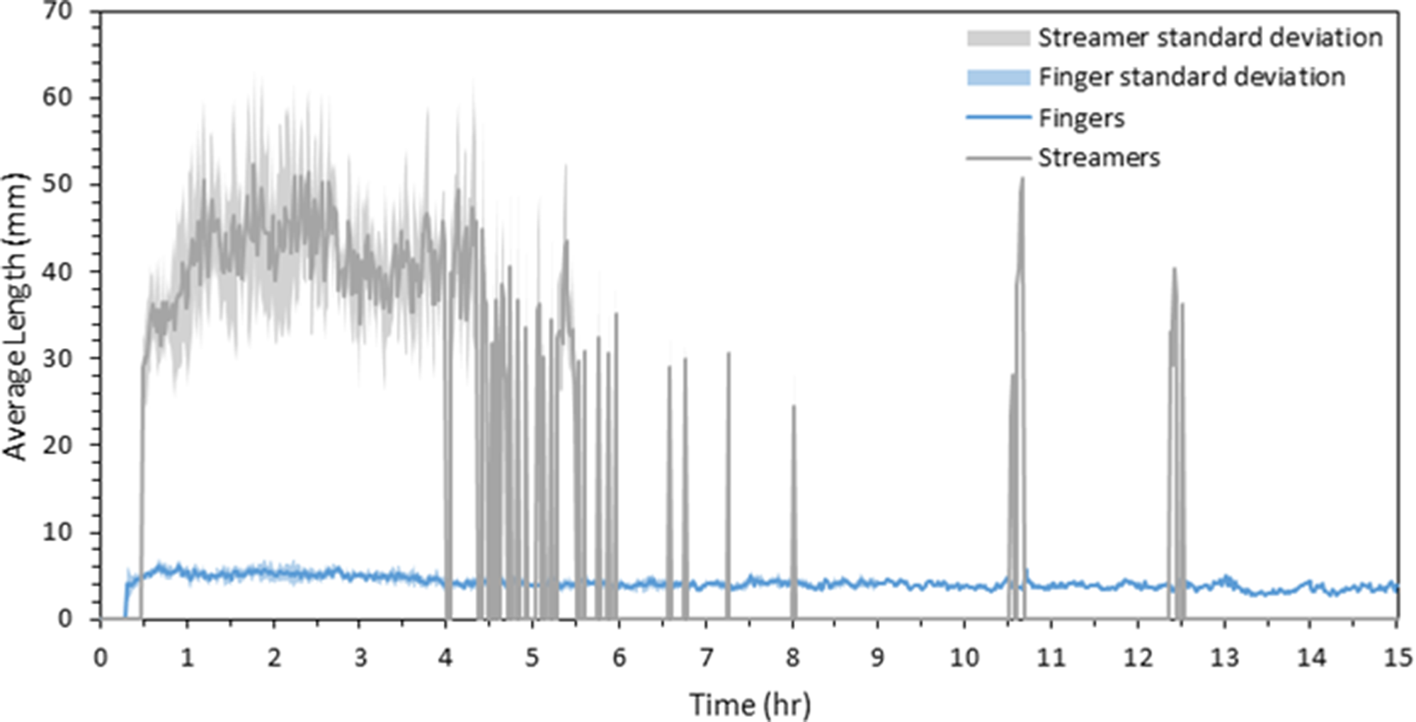
The average lengths of fingers are seen to be relatively stable over the 15-h duration, fluctuating around a mean of 4.11 mm (± 0.57 mm). In plotting the PDF, we see that on average, fingers are largely constrained to lengths below 10 mm, further reinforcing the choice of having a finger/streamer separation of at least 20 mm (Fig. S5a). Streamers, however, are seen to exhibit large fluctuations in their average length. Before 5 h, the average length of streamers fluctuates ∼40 mm (± 6.9 mm). Although the movements of the streamers and fingers are highly variable, they typically descend straight downwards (Fig. 4). However, after ∼4 h, the fingers are seen to slant to the right of the cell (Fig. 4e). As the experiment continues further, the streamer expulsions also tend towards the right (Fig. 4f). Although the fingers are thought to have a lower density and lower descent speeds compared to the streamers, their sheer number and eddy flow current seems to have an impact on the direction of the streamer flow, and this is evident in the average lengths of the streamers, which reduces after 4 h (Fig. 12).
Furthermore, after 5 h when the ice growth rate reaches its minimum, streamer lengths fluctuate largely and rapidly, between 0 and 50 mm without stabilizing around a specific value. We also see streamer lengths reaching its minimum, which indicates times when there are either smaller streamer expulsions or no streamer presence (when averaged length reaches zero). This indicates a slow-down of the brine channel streamer desalination activity with near-zero ice growth rate, which occurs after 5 h.
The PDF of the streamer average lengths show a Gaussian distribution, with the mode occurring between 38 and 45 mm (Fig. S5b). Since we note a timescale of significant interest (5 h), the PDFs before and after this timescale are also plotted. We see that although the distribution is still Gaussian, the tails before and after 5 h become inverted. We see larger probabilities of having a larger average length before 5 h (Fig. S5c) in comparison to after 5 h (Fig. S5d).
3.3.2.3. Mixing length
The mixing length represents the thickness of the sublayer within the IOBL, which is where the maximum amount of mass transfer from the interface is likely to be found. As defined by Middleton and others (Reference Middleton2022), the mixing length is the maximum expulsion from the interface, denoted by the most downward tip of the expulsions. The PDF of the mean length from all the experiments was plotted and further compared to the data obtained by Middleton and others (Reference Middleton2022) (Fig. 13a and b). As seen, both sets of data display a multimodal PDF of similar shape, with peaks occurring between 10–30 and 70–80 mm. This is the combination of two different stages: before 40 min, there is a higher probability of having smaller mixing lengths. Although the lengths reach maximum mean values of 100 mm, it is seen that after 40 min the distribution is Gaussian with short tails, which justifies the use of the maximum as a proxy for the mixing length. The probability of achieving a mixing length of 70–80 mm is the highest.
Probability density function of the mixing lengths from (a) the output obtained by Middleton and others (Reference Middleton2022) and (b) this study. To analyse the temporal evolution of the mixing lengths, the PDF of our experiments were plotted (c) before 40 min and (d) after 40 min into the experiment.
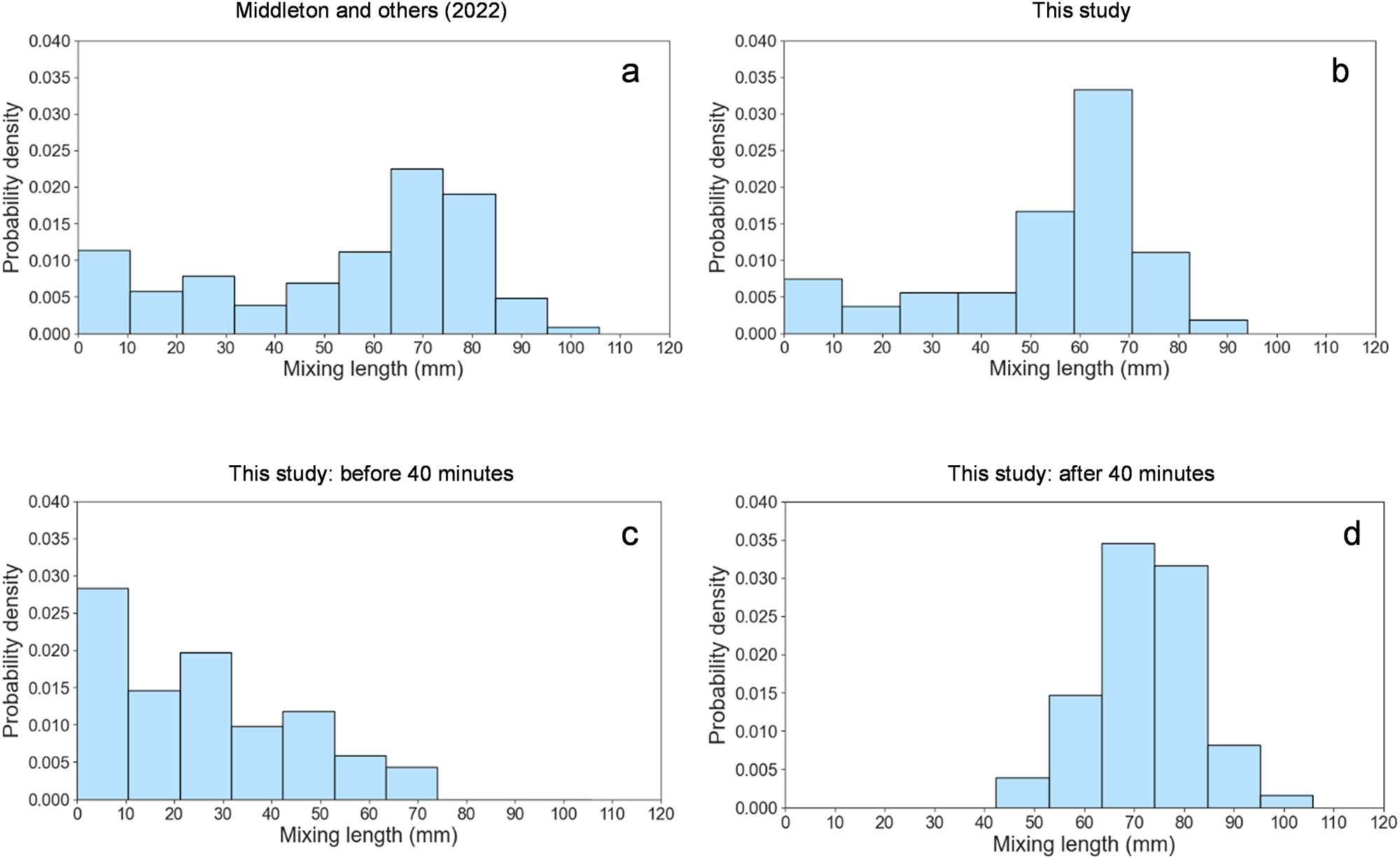
During the initial stages of the experiment, the mixing length is dominated by the finger’s length since there are no streamers present (see Figs 4 and 14a). However, after the initial 10–12 min, as the streamers begin to form, the total mixing length is seen to increase to the length of the streamers. The mixing lengths of the fingers remain consistent, while the mixing lengths of the streamers show large fluctuations between 30 and 100 mm for the analysed period. There is a slow initial expulsion of streamers that increases steadily until it fluctuates around a steady value (after 40 min) (Fig. 14a). This slow initial desalination could be linked to phenomena witnessed by Wettlaufer and others (Reference Wettlaufer, Worster and Huppert1997), who concluded that significant salt loss only occurs after a specific thickness is reached. Although the mixing lengths have large fluctuations, the mean value seems to stabilize ∼65 mm, corresponding to an experimental time of 60 min and an ice thickness of 20 mm. This suggests that initially, there are smaller amounts of desalination, which further increases until it reaches an ice thickness of 20 mm, thereafter the desalination stabilizes.
Comparison of the mean mixing length from (a) the DIP algorithm and (b) the manual calculations performed by Middleton and others (Reference Middleton2022), during the first 90 min if the experiments. The standard deviation of the three experiments is displayed as the shaded region surrounding the mean.
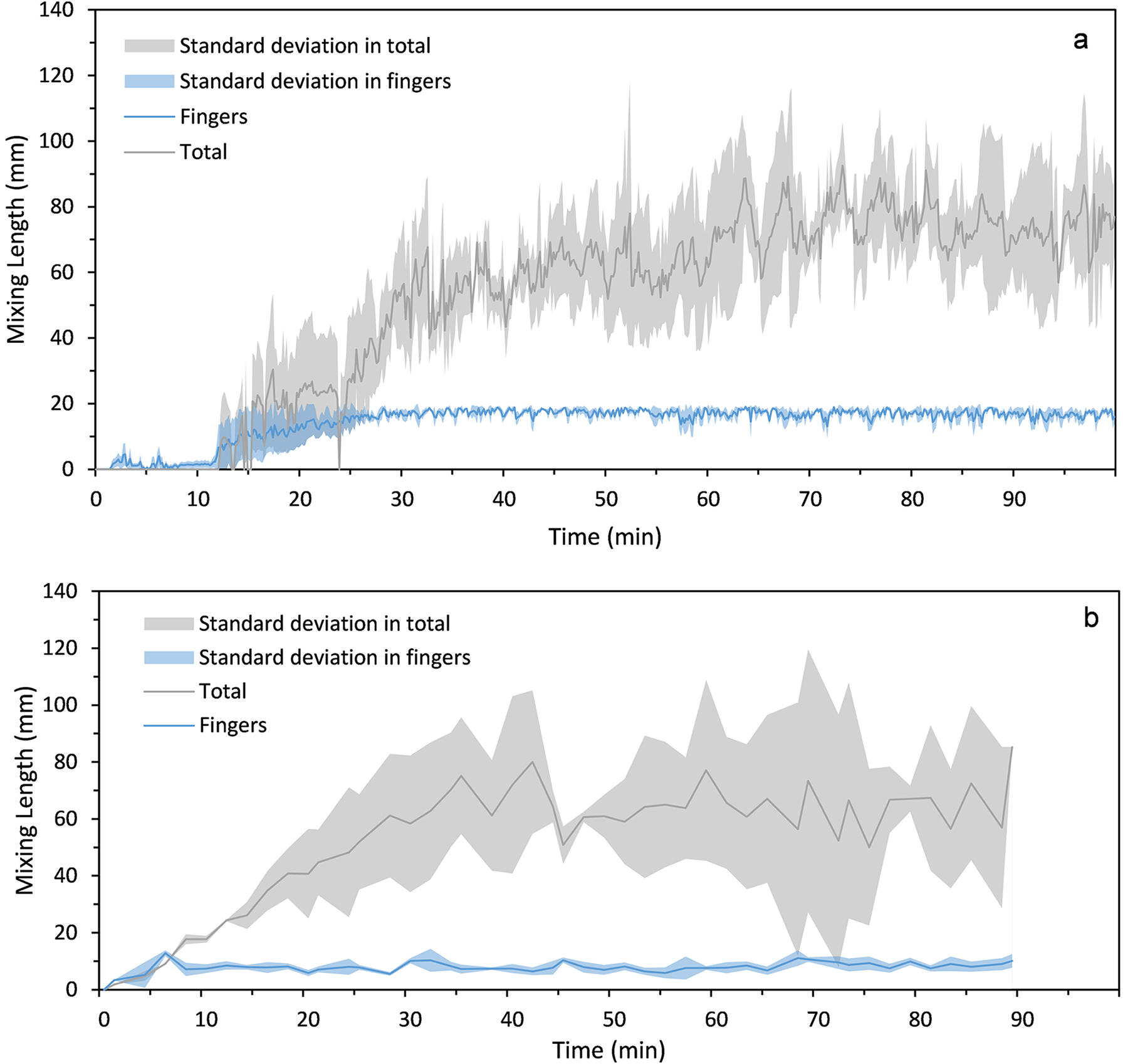
The mixing length obtained from the proposed DIP algorithm was further compared to the mixing lengths obtained from Middleton and others (Reference Middleton2022) (Fig. 14b). We see fluctuations in the mixing length in both datasets, which suggests periodic changes in the brine channel flow. Martin (1970) suggested that brine channels exhibit primarily downward flow, with some upward flow of less dense water. This could explain the oscillatory behaviour seen in the mixing lengths in Figure 14, where there is a general increasing trend in the mixing length, with periodic and sudden decreases in the length. Although we see similar overall trends, the higher sampling frequency of the DIP algorithm highlights a specific timescale where the dynamics of the system changes (40 min), which is difficult to see at the smaller sampling frequencies due to the higher variability. In using the algorithm, there is a significant reduction in the variability of the mixing lengths across the three experiments and a more consistent trend can be witnessed. Additionally, at the higher sampling frequency, we can see rapid oscillations at an approximate period of 5 min, which are barely visible in the low-resolution measurements (Fig. 14b). These fluctuations also show that in the absence of induced turbulence, the sublayer may indeed not be diffusive, as is assumed in many numerical models. The oscillations will be further investigated to determine how the frequency changes as a function of environmental conditions.
3.3.2.4. Average speed of fingers and streamers
As described by Middleton and others (Reference Middleton2022), only the descent speeds of the expulsions may be measured. This is a manual task that has not been improved yet, and it was performed at the same ice thickness as the ones used in Middleton and others (Reference Middleton2022) (32.5, 48.8, 60.3, 69.9 and 80.1 mm), to allow for a direct comparison. Using the streamer tracking algorithm, the descent speeds for six streamers and fingers for each of the three experiments were determined. Each expulsion is taken as an average of three expulsions and an average of the three experiments were plotted, with the error bars denoting the standard deviation between the experiments (Fig. 15a). The fingers have lower descent speeds and range between 0.05 and 0.15 mm s−1 and there does not appear to be a constant trend. The streamers are seen to have large descent speeds and exhibit a larger variability in their speeds, ranging from 0.32 to 0.54 mm s−1. Overall, it seems that the descent speeds from the tracking algorithm are lower than the speeds determined by Middleton and others (Reference Middleton2022), especially when the ice growth rate slows down (Fig. 9b). The largest speed is also observed at 12 h (80 mm) in Figure 15a with the thicker ice, and the overall trend is different.
(a) Average descent speeds determined for six streamers (full symbols) and fingers (open symbols) from the DIP algorithm in this study compared to the average descent speeds determine by Middleton and others (Reference Middleton2022). (b) The average relative mass flux calculated from the streamers and fingers.
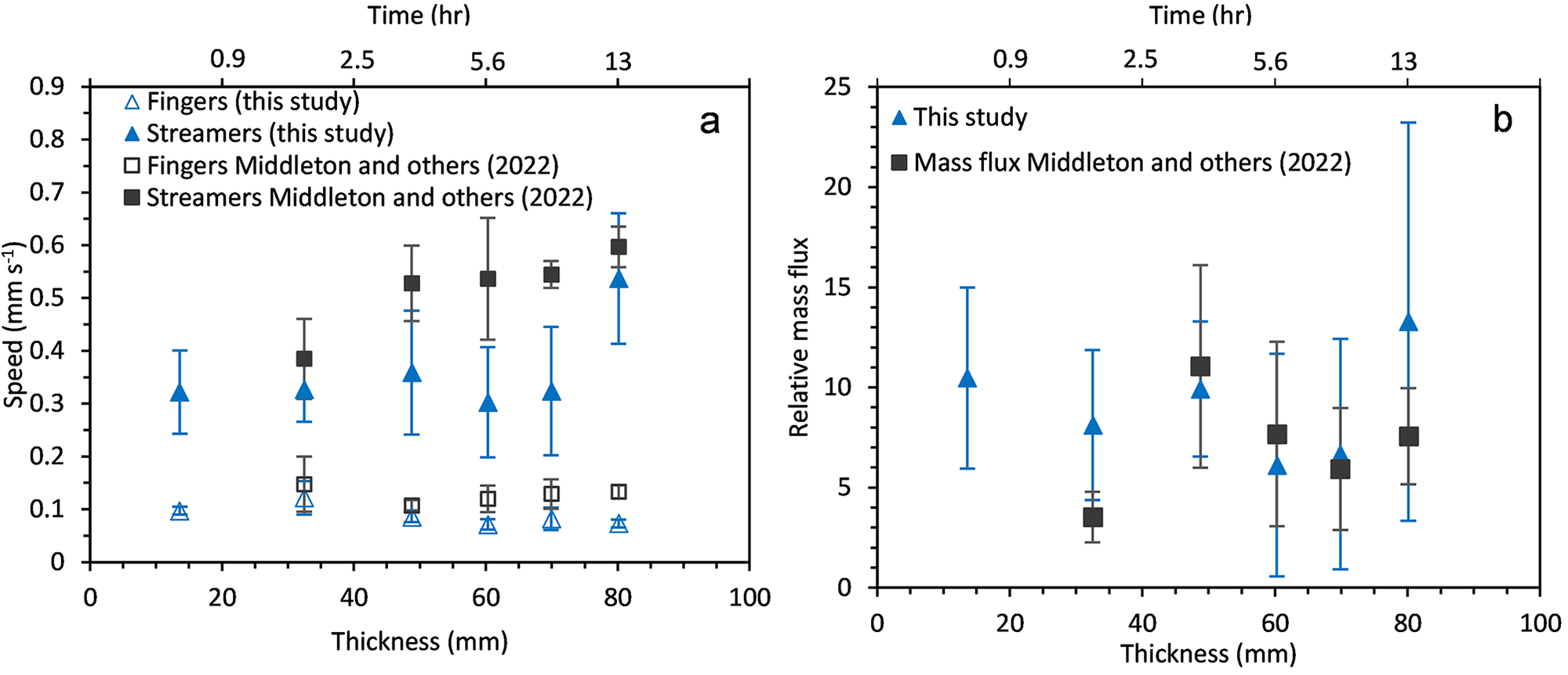
This difference in descent speed could be due to a bias in the manual results determined by Middleton and others (Reference Middleton2022). The streamer and finger speeds were determined by visually locating them within the image, and then calculating their speed based on the distance travelled and time taken. A bias could have been introduced, since visually, the most prominent or well-defined expulsion would have been chosen at any specific time, thereby not accounting for the less-defined expulsions with lower refractive index differences. By combining the information shown in Figures 11 and 12, we can infer a major change in features after 5 h: there is a significant decrease in the number of streamers, larger variability in the average length of the streamers and on/off behaviour, and there is a decrease in the speed of the streamers. We speculate that the latter is due to the fingers influencing the flow of the streamers within the eddy flow, making them slant as seen in Figure 4, and likely preventing a straight and quicker downwards descent. We thus see in the presence of low streamer rejections (i.e. after 5 h), the finger expulsions seem to have an impact on desalination and convective flows, proving their significance during the desalination process at low ice growth rates.
3.3.2.5. Relative mass flux of streamers and fingers
The relative mass flux of the streamers and fingers was initially determined using the equation proposed by Middleton and others (Reference Middleton2022), which is firstly, based on the assumption that the convective shape is cylindrical and secondly, based on the average radii of expulsions, which indicates that the square radii of streamers are twice that of fingers:
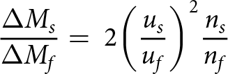 \begin{equation}\frac{{\Delta {M_s}}}{{\Delta {M_f}}} = {\text{ }}2{\left( {\frac{{{u_s}}}{{{u_f}}}} \right)^2}\frac{{{n_s}}}{{{n_f}}}{\text{ }}\end{equation}
 In eq. (2),  ${u_s}$ and ${u_f}{\text{ }}$refers to the expulsion speed and ${n_s}$ and ${n_f}$ to the numbers of the streamers and fingers, respectively. The results of our DIP output are compared with the Middleton and others’ (Reference Middleton2022) results in Figure 15b. The mass flux ratio fluctuates between 6 and 13. In the absence of high streamer activity, fingers have a significant impact on the desalination, and this is seen between an ice thickness of 32 and 50 mm (5 and 10 h), where there are fewer mass flux ratios and a lower ice growth rate. Similar observations were made by Middleton and others (Reference Middleton2022), where they have seen periods of interfacial convection dominating at low mass flux ratios. However, after an ice thickness of 60 mm (11 h), there are fewer streamers present, and the mass flux ratio seems to be in the range of 6–8 (which is in the lower range of ratios), with the exception of the high mass flux ratio occurring at 80 mm. There is however a large standard deviation; thus, this high value could be attributed to an outlying data point.
Obtaining the relative mass flux based on the requirements outlined by Middleton and others (Reference Middleton2022) (tracking the descent of a single streamer and finger at the same time, showing the tip of rejection) only provides a few data points since it has to be conducted manually to ensure that the conditions are met. This may not show the true dynamic behaviour of the system over the whole experimental period. It is unfeasible to obtain more data points manually, although this would provide a better approximation to the system. We can however get an average mass flux ratio over the whole experimental period, by further simplifying the calculation of the relative mass flux by expanding the descent speed into a change in distance ( $\Delta x$) over time ( $\Delta t$) for the streamers and fingers, respectively:
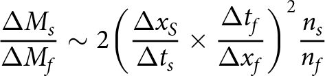 \begin{equation}\frac{{\Delta {M_s}}}{{\Delta {M_f}}}\sim 2{\left( {\frac{{\Delta {x_S}}}{{\Delta {t_s}}} \times \frac{{\Delta {t_f}}}{{\Delta {x_f}}}} \right)^2}\frac{{{n_s}}}{{{n_f}}}\end{equation}
If we consider a change in the average length of fingers and streamers in consecutive images, the difference in time for fingers and streamers will be the same (since the timelapse images were taken at 0.1 fps, leading to a constant 10 s between each consecutive image), simplifying the mass flux ratio to:
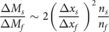 \begin{equation}\frac{{\Delta {M_s}}}{{\Delta {M_f}}}\sim 2 {\left( {\frac{{\Delta {x_s}}}{{\Delta {x_f}}}{\text{ }}} \right)^2}\frac{{{n_s}}}{{{n_f}}}\end{equation}
Obtaining a continuous relative mass flux based on the growing of streamers (as defined by Middleton and others (Reference Middleton2022)) is not possible, since there are times when the expulsions slow down—and even stop. However, if we extend the relative mass flux to include the increase in average expulsion length (when there is an increase in length from one expulsion to the next, i.e. an increase in the tip of displacement), we could determine the average relative mass flux, as seen in eq. (5). The length of the expulsions fluctuates, exhibiting periodic increases and decreases, thus to determine the average relative mass flux at the onset of streamer and finger expulsions (i.e. when both expulsions are seen to ‘grow’), only the lengths showing an increase in both the fingers and streamer lengths at the same timescales were used. This allows us to show the increase in length over time—and hence speed of descent and average relative mass flux ratio—of the expulsions.
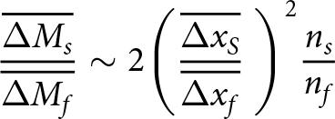 \begin{equation}\frac{{\overline {\Delta {M_s}} }}{{\overline {\Delta {M_f}} }}\sim 2{\left( {\frac{{\overline {\Delta {x_S}} }}{{\overline {\Delta {x_f}} }}{\text{ }}} \right)^2}\frac{{{n_s}}}{{{n_f}}}\end{equation}
 The average change in finger lengths are smaller than the change in streamer lengths, which would further leads to skewed mass flux ratios (since we are dealing with ratios, absolute length changes are not needed). The mass flux ratio was further normalized based on the respective lengths of the finger and streamer ( ${l_f}$ and ${l_s}$), leading to the use of eq. (6). These results are plotted in Figure 16 as a boxplot and are further compared with the manual results obtained in Figure 15b.
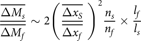 \begin{equation}\frac{{\overline {\Delta {M_s}} }}{{\overline {\Delta {M_f}} }}\sim 2{\left( {\frac{{\overline {\Delta {x_S}} }}{{\overline {\Delta {x_f}} }}{\text{ }}} \right)^2}\frac{{{n_s}}}{{{n_f}}} \times \frac{{{l_f}}}{{{l_s}}}\end{equation}
The average mass flux ratio as a function of binned ice thickness (eq. (6)) compared to the manually calculated mass flux ratio based on the descent speed (eq. (2)) using the DIP streamer tracking algorithm (blue triangle) and Middleton and others (Reference Middleton2022) (black square) as a function of ice thickness. Increasing bins are represented by the increased colour intensity (light to dark) and the corresponding points represent the outliers within each bin. The centre of the boxes represents the median, while the top and bottom of the box represents the upper and lower quartiles, respectively. The whiskers represent the upper and lower values of the dataset. The time is presented on the secondary x-axis.
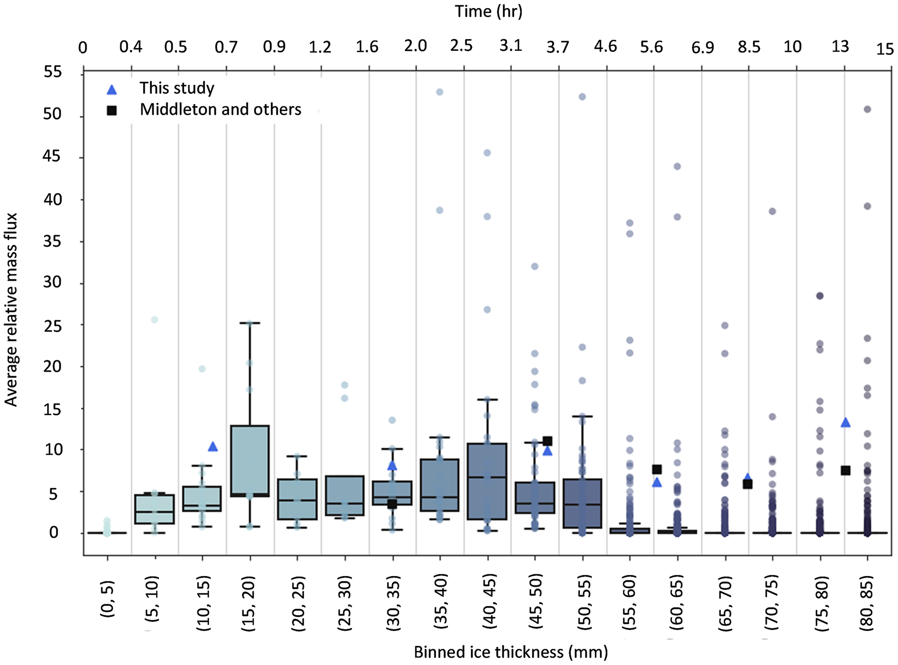
During the period when the streamers are ‘off’ (when there are no streamers present), the mass flux ratio is zero, indicating no contribution of streamers to desalination. At the beginning of the experiment, we see mass flux ratios of zero—this is consistent with Figure 11, where we see finger expulsions dominating at the beginning of the experiment with no streamer expulsions. Larger mass flux ratios indicate a large streamer contribution and minimal finger contribution, mostly due to either a small number of fingers present or a small average change in the downward movement of finger tips. The average relative mass flux varies largely and rapidly between 0 and 52. We can see that the most active period of streamer contribution occurs between an ice thickness of 5 and 55 mm (between 30 min and 5 h, as seen in Fig. 9). The median average mass flux ratio fluctuates between 2 and 7. This is on the lower bound of values determined by both sets of manual calculations. This could be due to the streamers that were chosen for the manual calculations being the most prominent visually, instead of being chosen randomly. The large number of outliers, ranging between 40 and 85 mm suggests that although the streamers do switch off, resulting in a lowered mass flux contribution, once they switch on, they have the potential to reach higher mass flux ratios, which seems to occur at the larger ice thickness.
In comparing this output with the manual results, we see that the manual results for both this study and Middleton and others (Reference Middleton2022) fall towards the upper bound of the boxplot tails for all points, except between a thickness of 30–35 mm, where it falls near the median. This overestimation may be due to again, the bias in choosing the most visually prominent expulsions during computation. This, coupled with the fact that only three expulsions were used for each thickness and only six different expulsions were used to understand the whole 15-h experimental period, makes it difficult to accept the manual outputs results. After an ice thickness of 55 mm, we further see a significant reduction in the heights of the boxes, showing that the bulk of the data points lie on the x-axis, i.e. zero mass flux ratio. This indicates a period of potential interest in which the dynamics of the system seems to change since we see a drop in the mass flux ratio, significant finger contribution to desalination and a decrease in the number of streamers (Fig. 11). As the experiment progresses towards its end, the underlying water becomes more saline as a result of the desalination occurring within this close system. The increase in water salinity might have an impact on the expulsion of deep reaching streamers, thereby impacting the way convection operates in this system. In extending the experimental parameters to include an open system, maintaining a constant underwater salinity or in monitoring the change in salinity from the beginning of the experiment (1 h) until the end (15 h), we could provide more insight into the change in the expulsion behaviour as a result of changes in the water salinity.
Although the average relative mass flux is on the lower bound in comparison to the two sets of manually calculated mass flux ratios, we see that the manual sets of data do fall within the ratios calculated autonomously. Using only three descent speeds for each finger and streamer (as is done using the tracking algorithm and by Middleton and others (Reference Middleton2022)) in an already highly dynamic system may not be completely representative of the system, thus using the increase in average length may be a better approximation due to both having a higher frequency of data and in avoiding the bias of using visually dominant streamers.
4. Summary and conclusions
Digital image processing techniques were developed to autonomously investigate the desalination processes of artificial sea ice in a quasi-2D Hele-Shaw cell. This set of steps allowed for successful isolation of finger and streamer expulsions, as well as automatic separation of their respective properties which is a substantial advancement as compared to previous studies.
Fingers are seen to have an impact on the streamer flow during the later parts of the experiments, where the eddy currents from the fingers influence the streamers into a sideward direction. Furthermore, fingers are seen to be active over the whole experimental run, while streamers are firstly, delayed during the beginning of the experiments, have a slow increase and then seem to decrease in number and length towards the middle and end of the experiments, which agrees with previous Rayleigh number calculations suggesting active convection in the early stages of ice growth. This further suggests that the influence of finger expulsions might become significant at slower growth rates during the latter parts of the experiments. It seems that the streamer activity is at a maximum and the most stable during the first 5 h of the experiment during maximal ice growth rate, after which the activity is seen to decrease significantly and the variability in the lengths are seen to increase. After 5 h of experimentation when ice growth rate has decreased significantly and is close to zero, the dynamics of the streamer behaviour in the system seems to change, where the streamers begin to exhibit an on/off behaviour, their descent speed is seen to decrease, and their flow direction becomes impacted by the fingers eddy currents. This suggests that not only are there instances where fingers are contributory to desalination (i.e. at low mass flux ratios), but they also impact streamer behaviour, potentially due to their large number of rejections in comparison to the low number of streamers rejected.
It is important to stress the potential shortcomings of the closed system Hele-Shaw cell experimental set-up. Firstly, the ‘slanting’ behaviour of fingers and streamers might have risen from the confined geometry of the set-up. Middleton and others (Reference Middleton, Thomas, De Wit and Tison2016) exhibited the meandering behaviour of brine channels within the Hele-Shaw cell. The slanting expulsions could be a result of this brine channel meandering across the horizontal plane, thereby changing the direction of flow. Secondly, and perhaps more importantly, working in a closed system significantly increases the salinity of the remaining water reservoir towards the end of the experiment, affecting the Rayleigh convection in a way that it decreases the salinity contrast between brines and the underlying reservoir, therefore hampering the convective process and the efficiency of desalination through the brine channel/streamers system. Indeed, implications of our experimental results for the ‘real world’ would be that beyond 10 cm of ice growth the desalination processes would be dominated by interfacial desalination, which is not supported by, e.g. the Rayleigh numbers calculated for the bottom 10 cm of actively growing sea ice in some field studies (e.g. Tison and others, Reference Tison2020). An improvement of the experimental set-up for future work, would be to allow recirculation of the remaining liquid in the cell from an external reservoir of constant salinity, kept just above the freezing point.
The advantage of using the autonomous algorithm is that data points can be continuously extracted from each individual frame, allowing for the continuous analysis of finger and streamer behaviour—and hence internal and interfacial convection—which could not previously be conducted. This further allows us to infer differences in the dynamics of the system, based on the time period and ice thickness. Where streamer activity is at a maximum, this indicates a dominant period of gravity drainage, which slows down after the slowdown of the sea-ice growth rate. Interfacial-driven salt segregation, however, is seen to be active over the whole experimental period and becomes more dominant after a decrease in streamer activity (after 5 h and an ice thickness of 55 mm).
Based on the output, the manual mass flux ratios of this study are slightly lower than the mass flux ratios determined by Middleton and others (Reference Middleton2022); however, although both sets of manual results fall within the range of the autonomously determined results, it does seem to result in a slight overestimation. We can see that choosing specific and limited expulsions from the Schlieren image, based on inspection, could lead to a bias further resulting in us inferring larger mass flux ratios. Using the autonomous method, we can see many more data points that lie close to a mass flux ratio of zero after an ice thickness of 55 mm. This provides a better understanding and more statistically trustworthy set of results reflecting the contribution of internal and interfacial convection over the experimental period. The output of this algorithm provides a visual analysis of the phenomena witnessed by Wettlaufer and others (Reference Wettlaufer, Worster and Huppert1997) and Martin (Reference Martin1970), showing both the delay in desalination and the variability in the expulsion of brine through the channels, with the potential brief uptake of less dense water as seen in the mixing length. Expanding on the experimental output of convection near and below the interface is vital, since there are a limited number of laboratory- and field-based experimental studies currently available, which can be used as a comparison to numerical models. The experimental methods to visualize the expulsions in this study are limited to a controlled laboratory-based environment due to the need for the complex Schlieren optical set-up to be used, which cannot be deployed in the field. However, in combining the methods used in this study with measurements such as temperature and parameters such as solid fraction, bulk salinity and Rayleigh number (authors are currently developing methods for experimentation), we will link the visual aspects of desalination to the quantitative aspects. These quantitative aspects can thus be used as a comparison to field investigations and can further be implemented into parameterizations for numerical modelling.
Although this is an extension of Middleton and others (Reference Middleton2022), we have demonstrated that we built a method that allows for the statistical analysis of the distribution of the average- and mixing-lengths, which was not previously able to be achieved, while also eliminating the bias associated with choosing specific data points. The fluctuating mixing length shows that in the absence of induced turbulence, there is no laminar layer, which directly opposes the widely accepted theory that the sublayer beneath the ice–ocean interface is diffusive. Within the context of the broader cryosphere community, these results can help refine parameterizations and numerical models relating to sea ice. The laboratory- and field-based work performed by Notz and others (Reference Notz, Wettlaufer and Worster2005) and Notz and Worster (Reference Notz and Worster2009) is vital to numerical models; however, they lack the advantage of this study in obtaining measurements close enough to the interface to investigate the sublayer in more detail. We demonstrate a way to visualize the sublayer in the absence of turbulence, which cannot currently be obtained in situ. This is highly advantageous, since we can see that the sublayer—which has widely been assumed to be diffusive—is more turbulent. This has a great impact on the current numerical models used to determine the ablation and melting of sea ice. Lastly, we have demonstrated the contribution salt segregation (fingers) has in the absence of (or at minimal amounts of) gravity drainage (streamers) and that it does indeed have an impact on desalination.
The system is highly dynamic, showing periodic changes in both the fingers and streamers. Since we have shown that the DIP method allows for continuous and autonomous investigation of convection, additional future work could use the algorithm to investigate the changes in periodicity at various conditions to determine if the dominant period of gravity drainage changes. To refine the algorithm and obtain the mass flux ratios based on the descent speed of individual streamer and finger expulsions, implementation of machine learning methods, with an emphasis on model training to identify the expulsions, will be valuable. The behaviour of expulsions changes rapidly (slanting, starting, stopping, merging, etc.). Thus, a model trained to identify these dynamic behaviours would be greatly beneficial to improve the tracking of expulsions.
Supplementary material
The supplementary material for this article can be found at https://doi.org/10.1017/jog.2025.10066.
Data availability statement
The videos mentioned in the supplementary material can be found at https://doi.org/10.5281/zenodo.15393780. The scripts used in this paper can be found at https://github.com/safiyyah97/Developing-Digital-Image-Processing-methods-for-Schlieren-Images.git. The data reported in this manuscript are available upon request; other data used for comparison are described in Middleton and others (Reference Middleton2022).
Acknowledgements
This work is based on the research supported in part by the National Research Foundation of South Africa (NRF Grant No: 118745 and 116801). This work has received funding from the European Union’s Horizon 2020 research and innovation program under grant agreement No 101003826 via project CRiceS (Climate Relevant interactions and feedbacks: the key role of sea-ice and Snow in the polar and global climate system). We would like to thank the research office at the University of Cape Town for their financial support. This publication is based on research that has been supported in part by the University of Cape Town’s Research Committee (URC). The experimental work has been conducted at the Université libre de Bruxelles (ULB). We thank Patrick Grosfils for discussions and Adam Chafai for help with the Schlieren set-up.
Author contributions
S.M.: Investigation, DIP Methodology, Formal analysis, Visualization, Software, Writing—original draft.
M.V.: Writing—review & editing, Formal analysis, Visualization, Funding acquisition.
F.F.: Conceptualization, Experimental Methodology, Visualization, Resources, Writing—review & editing.
J.L.T.: Conceptualization, Experimental Methodology, Visualization, Writing—review & editing.
A.D.W.: Conceptualization, Experimental Methodology, Visualization, Resources, Writing—review & editing.
T.R.: Conceptualization, Visualization, Resources, Writing - original draft, Writing—review & editing, Supervision, Funding acquisition.


 Open access