


INTRODUCTION
Dengue, an infection caused by flavivirus, transmitted by arthropods of the genus Aedes, is prevalent in different parts of the world, and constitutes one of the major public health problems in many tropical and subtropical regions where Aedes aegypti and other suitable mosquito vectors are present.
Current dengue control measures use entomological surveillance with the aim of detecting changes in adult or immature A. aegypti populations. Therefore, to prevent dengue disease, public health policy relies on the control and eradication of the mosquito A. aegypti. In order to prevent dengue outbreak, periodic surveys designed to detect changes in key adult indices play an important role since they allow detection of fluctuations in the adult population, which may prompt changes in vector control strategy. For this reason regular random inspections are made to control breeding habitats: oviposition traps are put in place, urban premises are inspected and breeding sites are either emptied or treated with Temephos depending on their size. However, ecological, behavioural and control information on population size, distribution, survival, seasonal abundance and insecticide susceptibility are required for an understanding of the epidemic potential and formulation of control strategies [Reference Monath1].
In the present study we address the question regarding the population size of A. aegypti by developing a simple mathematical model. In population dynamics theory, the size of a population is determined if it is possible to estimate the parameters describing the complex relationships existing among the stages that comprise the population. In the case of A. aegypti, the life-cycle encompasses two different environments, for this reason the size of the mosquito population can be determined by combining in a mathematical expression the parameters that describe the passage along the aquatic (encompassing egg, larval and pupal stages) and adult (winged) phases. With the aim of assessing the size of the A. aegypti population based on the parameters applicable to the mosquito's life-cycle, we designed temperature-controlled experiments, and based on these data, we estimated the entomological parameters. The knowledge of how the size of the mosquito population varies with temperature helps in the choice of an appropriate strategy from the available controlling mechanisms [Reference Yang and Ferreira2], which are mechanical (removing of breeding sites) and chemical (larvicide and insecticide). Our goal was to estimate the rates of mortality in the whole aquatic phase (comprising larvae and pupae) and in adult mosquitoes. Moreover, we estimated the rate of emergence of adult mosquitoes from hatched eggs that survived the larval and pupal stages. In the literature we found laboratory experiments that assessed the effects of temperature on A. aegypti (see e.g. [Reference Rueda3–Reference Tun-Lin, Burkot and Kay5]). However, the entomological parameters estimated in a broad range of temperatures can provide the trend of the number of mosquitoes with temperature, which is essential to prevent an increase in the size of the mosquito population.
The paper is structured as follows. The next section describes a simple deterministic model of the growth of the mosquito population followed by presentation of the experiment design and fitting method. Next follows a section on the adjusted entomological parameters and the link between population dynamics of mosquitoes. Then there is a section on the estimated temperature-dependent rates and in the final section we discuss the results and present conclusions.
MODELLING DYNAMICS OF THE MOSQUITO POPULATION
In this section we develop a simple mathematical model to deal with the mosquito population taking into account the entomological parameters estimated from temperature-controlled experiments, which are described in next section.
The dynamics of the vector population are based on the life-cycle of the mosquito A. aegypti, which comprises egg phase, two successive aquatic phases (larval and pupal) and one adult form. However, we simplify the life-cycle by allowing the larval and pupal stages to constitute one compartment in the modelling, designated the aquatic phase, while the adult form comprises only female mosquitoes. Here we assume that there are sufficient male mosquitoes to mate with females; moreover, 24 h after emergence, the females are able to copulate and the sperm is stored throughout their lifespan with the eggs being fertilized as they are formed. Hence we can disregard the male population in the modelling, assuming that all female mosquitoes have effectively copulated. The number of female mosquitoes at time t, designated by M, increases according to the per capita rate at which pupae emerge from the aquatic phase πq, and decreases according to the per capita mortality rate μf. The number of aquatic forms at time t, designated by A, increases with the per capita oviposition rate φ (1 – A/C), where φ is the intrinsic oviposition rate, C is the carrying capacity and (1 – A/C) is the available capacity of the recipients to receive eggs; and decreases according to the change of pupae into adult mosquitoes and death, described, respectively, by the emerging rate πq and the per capita mortality rate μq. Neither do all eggs hatch to larvae, nor do they all produce female mosquitoes. For this reason we introduced the fraction of eggs hatching to larvae k, with 0<k<1, and the fraction of female mosquitoes hatched from all eggs f, with 0<f<1.
The passage from egg to aquatic phase until reaching the winged form can be quantified using the above description regarding the two stages of the mosquito population and their respective parameters. By balancing the flows through the stages, we obtain the dynamics of the mosquito population, which can be described by the following ordinary differential equations
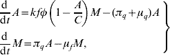
where all the entomological parameters are temperature-dependent. To incorporate the temperature-dependent feature into the entomological parameters, we allow the temperature T be a function of time, i.e. T(t). By doing this, we are taking into account the seasonal variation in the entomological parameters [Reference Yang and Ferreira2]. For instance, the mortality of female mosquitoes can be set as μf=μf(T), according to the seasonal variation T(t)= +T 0 sin(2π/365)t, where is the mean annual temperature and T 0 is the amplitude of the temperature variation.
If the entomological parameters are described by the annual mean temperature , equation (1) can reach one of two stationary regimens, called equilibrium points. One is designated as trivial (absence of mosquito population), which is given by Ā=0 and  =0; and the other as non-trivial, given by
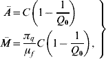
where the basic offspring number Q 0 is given by
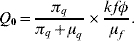
The basic offspring number Q 0, is a key parameter in population dynamics theory. Depending on this value, the stationary regimen can be either a trivial (Q 0⩽1) or non-trivial (Q 0>1) equilibrium point (see Appendix A).
The parameter Q 0 deserves a biological interpretation. Note that 1/μf is the average survival time of a female mosquito and fφ/μf is the average number of ‘female’ eggs produced by a female mosquito during her entire lifespan. Of these eggs, only a fraction k hatch to larvae, and kfφ/μf is the number of potential larvae that become female adults. In the aquatic phase, 1/(πq+μq) is the average survival period in this phase (the removals include passage to the adult stage and mortality of the aquatic form, which encompasses larvae and pupae), while 1/πq is the average time elapsed from the eggs hatching until they reach the adult stage. Hence, πq/(πq+μq) is the probability that a hatched egg survives during the whole aquatic stage, and enters the adult stage. Therefore, Q 0 is related to the eggs laid by one female mosquito and to the probability that these hatched eggs survive the whole aquatic stage and become female mosquitoes. In summary, Q 0 provides the mean number of viable female offspring produced by one female mosquito during her entire time of survival.
In next section we describe temperature-controlled experiments in order to assess the entomological parameters.
EXPERIMENT DESIGN AND ESTIMATION METHODS
In order to estimate the entomological parameters of A. aegypti's life-cycle, we designed temperature-controlled experiments. The data yielded from each temperature-controlled experiment were adjusted for the parametrized functions. We describe the experiments performed for different temperatures and the estimation methods applied to the collected data.
Experiment design
Temperature-controlled experiments were designed to assess the effect of temperature on the development and survival of immature (aquatic) forms and the survival and oviposition of adult A. aegypti mosquitoes. In each experiment, a fixed number of larvae or mosquitoes were placed in a germination chamber where the temperature was regulated (the device did not allow for the control of humidity). The A. aegypti strain used in the tests was captured from the city of Marìlia (−22° 12′ 50″ latitude, 49° 56′ 45″ longitude, 350 km from the city of São Paulo), situated in the northwest of São Paulo State, Brazil.
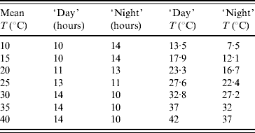
The light inside the germination chamber was programmed to simulate the naturally occurring seasonal photoperiod. The period of 1 day was divided into ‘day’ (light on) and ‘night’ (light off), according to the photoperiod that occurs in the city of Marìlia. In low temperatures the dark period lasted longer than the light period to mimic the winter season, and vice versa for high temperatures. Inside the germination chamber two temperatures were fixed, corresponding to the light and dark periods. The weighted (regarding length of time when the light was turned on or off) mean temperature was taken as the temperature of the experiment, which is summarized in Table 1. However, in order to check if the programmed temperature was achieved during each experiment, a thermohygrograph was positioned inside the chamber. Temperature and humidity data were then recorded on a weekly basis. The weekly data were then transcribed and gave the weighted average temperature; this temperature was taken as the real temperature inside the germination chamber, instead of the programmed one.
Weighted average temperatures (mean) programmed in the germination chamber for the periods of time (in hours) that the light is turned on (‘day’) and off (‘night’)
To estimate the mean survival time of adult mosquitoes the experiment consisted of following up from their emergence from pupae, from which the mortality rate was derived, as well as the number of eggs laid at each temperature. A total of 100 female and 30 male newly emerged mosquitoes were placed in a cage containing an amber glass with a filter paper for egg-laying. Inside the cage necessary food (water with honey) was available ad libitum, and once a day the mosquitoes received a bloodmeal from an immobilized mouse in order to allow the development of the fertilized eggs. The eggs that were laid on the filter paper were counted every day, and the filter paper was then substituted. The number of surviving male and female mosquitoes was also recorded every day. This aim of this temperature-controlled experiment was to evaluate the influence of temperature on longevity and on one aspect of fertility, i.e. egg production. The experiment was performed from 16 August 2002 to 12 December 2004.
The aquatic phase dealt with survival time and length of time spent in the larval and pupal stages at different temperatures. We selected 100 newly hatched eggs, in the first instar larvae, which were placed in a bowl inside the germination chamber with food (fish) freely available. When the fourth instar larvae turned into pupae, they were transferred to individual hearing vials with caps and remained inside the chamber. The observation period continued until the emergence of the adult mosquito. As in the previous procedure, the numbers of dead immature as well as instar changes to the next stage were recorded every day. However, in the experiment at the temperature of 10°C we proceeded as follows: we allowed the larvae to emerge at stages L2, L3, L4 and pupate at a favourable temperature (25°C), and then exposed them to 10°C. This temperature-controlled experiment was performed from 21 January 2004 to 25 July 2005.
The experiments performed in the germination chamber were designed to measure the effects of temperature on the development and survival at different stages of the mosquito's life-cycle. For this reason follow-up began with the first larval stage and not with eggs because, except for temperature, the hatchability of eggs is influenced by many factors, e.g. poor embryonal development and desiccation. Each of the experiments described for immature and adult mosquitoes were repeated, respectively, with three and two observations for each temperature range.
Estimation of the parameters
Data collected from temperature-controlled experiments were fitted taking into account the probability of maintaining the original state and the probability density for change of state. These functions are parametrized in terms of the parameters τ and β, which are, respectively, the half-time and heterogeneity degree. The half-time is the observation time at which the probability of the original state being maintained is 1/2, and the heterogeneity degree measures how the change of state occurs broadly scattered in the observation times. The probability distributions are described in Yang et al. [Reference Yang6].
Briefly, the probability of maintaining the original state at observation time a is given by
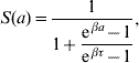
where at a=0 the follow-up is initiated. This function was obtained with regard to biological conditions which were taken as weights. The probability density for change of state at observation time a is
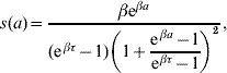
from s(a)=−dS(a)/da. We hereafter refer to the probability of maintaining the original state S(a) as ‘maintaining probability’ and refer to the probability density for change of state s(a) as ‘changing probability’. Individuals (a generic term referring to larvae, pupae and adult mosquitoes) in each follow-up experiment have different behaviours, and distinct phenomena are described by different scales of observation times, which are measured by the heterogeneity degree β and half-time τ, respectively.
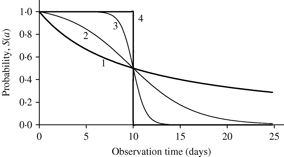
Figure 1 shows the shape of maintaining probability S(a), together with two extreme probabilities: all individuals behaving completely homogeneously (the value of β is extremely high or, β→∞, indicated by 4), where for a<τ, S(a)=1; otherwise, S(a)=0, and completely heterogeneously (the value of β is extremely low or, β→0, indicated by 1), governed by the equation S(a)=1/(1+a/τ). The half age τ was arbitrarily fixed at 10 days. Different behaviours of individuals in each experiment can be matched by a curve situated between these two extreme curves. For instance, intermediate heterogeneous and homogeneous behaviours are illustrated using, respectively, the values β=0·5 day−1 (indicated by 2) and β=3·0 days−1 (indicated by 3).
The probability of maintaining the original state as a function of observation time is shown for 4 heterogeneity degrees (days−1): (1) β→0, (2) β=0·5, (3) β=3·0 and (4) β→∞. The common half time is τ=10 days.
The experiment consists of the follow-up of n individuals, in which the occurrence of transition or censoring is registered at the observation time. The parameters τ and β are fitted by the nonlinear likelihood estimation method based on the set of recorded data Ω={(a i, ωi)}, i=1, 2, …, n, where the index i stands for the observation of the i-th individual and ωi is the outcome at observation time a i. The fitting method is described in [Reference Yang6].
The probability functions [equations (4) and (5)] are applied to estimate entomological parameters of the mosquito's life-cycle. For adult mosquitoes we estimated the parameters τ and β describing the survival time: the time elapsed from the emergence of the mosquito until its death. The parameters regarding survival time can also be estimated for the aquatic form. However, besides the survival phenomenon, the same set of data are used to estimate τ and β describing transition time: the time elapsed from the hatching of the egg until the emergence of the adult mosquito.
For adult mosquitoes, censored individuals are those lost at each day's count. Moreover, the remaining mosquitoes at the last day of observation (end of the experiment) are considered censored. The figure is completely different regarding aquatic forms; larvae and pupae do not escape and ultimately change to the next stage. The censoring is, then, defined according to the phenomenon: in the survival study, the number of larvae emerging as adult mosquitoes is considered censored; while in the transition study, the number of dead larvae and pupae is taken as censored. The observation time can be understood as the age of the mosquito or, in the case of the aquatic phase, the age of the immature form.
Each set of follow-up data from different temperature-controlled experiments is fitted considering the probability functions S(a) and s(a), given by equations (4) and (5), which are applied to, respectively, censored and transition data. In Appendix B we present only the fitted parameters omitting the corresponding curves, because the shapes of all adjusted curves are situated between the extreme curves shown in Figure 1.
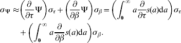
Once we estimated the parameters τ and β, we could calculate the average length of time of remaining in the original state η or the average time elapsed before changing to the next stage ξ (both are generically represented by Ψ) according to
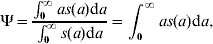
where  . The parameters η and ξ are designated, respectively, the survival time and the transition time (time spent in a specific stage). The corresponding error [Reference Frank7] is calculated from
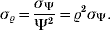
The mortality rate μ or the transition rate π (both are generically represented by ϱ) for survival time and transition time, respectively, can be approximated by

and the corresponding error [Reference Frank7] as
In Appendix B the calculated average periods of time and the mortality and transition rates are given.
ADJUSTING THE TEMPERATURE-DEPENDENT ENTOMOLOGICAL PARAMETERS
The mortality and transition rates, as well as the oviposition rate, were calculated for different temperatures. To adjust these temperature-dependent entomological parameters we chose a polynomial of degree m,
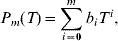
where T is the temperature (in °C) and the coefficients b i, with i=0, 1, 2, …, m, are fitted by the linear least squares estimation method [Reference Press8], which minimizes χ2,
![\chi ^{\setnum{2}} \equals \sum\limits_{j \equals \setnum{1}}^{N} {\left[ {{{P_{m} \lpar T_{j} \rpar \minus \varphi _{j} } \over {\sigma _{j} }}} \right]^{\setnum{2}} \comma }](https://static.cambridge.org/binary/version/id/urn:cambridge.org:id:binary:20160921000207967-0817:S0950268809002040:S0950268809002040_eqnU3.gif?pub-status=live)
where φj is the mortality or transition rate at temperature T j, with σj being the corresponding error, and N is the total number of observed rates. In Tables 5 and 10 (Appendix B) there are rates assuming zero value, in which case we arbitrarily set σ=10−6, because at extreme temperatures there are neither oviposition nor transition to winged form. The degree of the polynomial m must be chosen appropriately. As the degree of the polynomial increases, the better becomes the fit because the value of χ2 is lowered. However, increasing the degree of the polynomial can increase the number of extrema or/and generate negative values to the polynomial function. Bearing these features in mind, we present the curves of the chosen degree of the polynomial plus the nearest degrees.
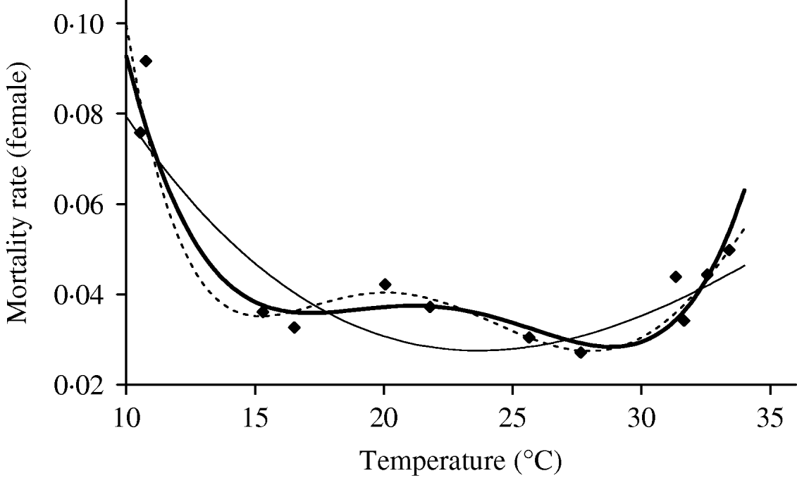
We deal first with the adult mosquitoes. Based on Table 4 (Appendix B), we fit the mortality rate as a function of temperature. Figure 2 shows the temperature-dependent mortality rate of female mosquitoes. Ignoring the small fluctuation, we observe a basin-shape for optimal survival of mosquitoes, i.e. a small mortality rate around the range 15<T<30°C. Close to the lower and the upper bounds the mortality rate increases quickly.
The fitting of the female mosquito mortality rate as a function of temperature. The estimated coefficients b i with errors in parentheses [days−1×(°C)–i] are: b 0=8·692×10−1 (1·291×10−1), b 1=−1·590×10−1 (2·698×10−2), b 2=1·116×10−2 (2·004×10−3), b 3=−3·408×10−4 (6·297×10−5) and b 4=3·809×10−6 (7·114×10−7) (–––). Fittings for the third- (- - -) and fifth- (–––) degree polynomials and the observed values (◆) are also shown.
Based on Table 5 (Appendix B), we fit the oviposition rate as a function of temperature. Figure 3 shows the temperature-dependent oviposition rate. For temperatures up to 30°C, the oviposition rate increases quasi-linearly, after which it enters the decreasing phase, which is abrupt after 35°C. For T<10·57°C, the negative values must be changed to zero. We assume φ=0 and σφ=10−6 as the temperatures at which female mosquitoes do not lay eggs.
The fitting of the oviposition rate as a function of temperature. The estimated coefficients b i with errors in parentheses [days−1×(°C)–i] are: b 0=−5·400 (2·969×101), b 1=1·800 (7·866), b 2=−2·124×10−1 (7·382×10−1), b 3=1·015×10−2 (2·869×10−2) and b 4=−1·515×10−4 (3·886×10−4) (–––). Fittings for the third- (- - -) and fifth- (–––) degree polynomials and the observed values (◆) are also shown.
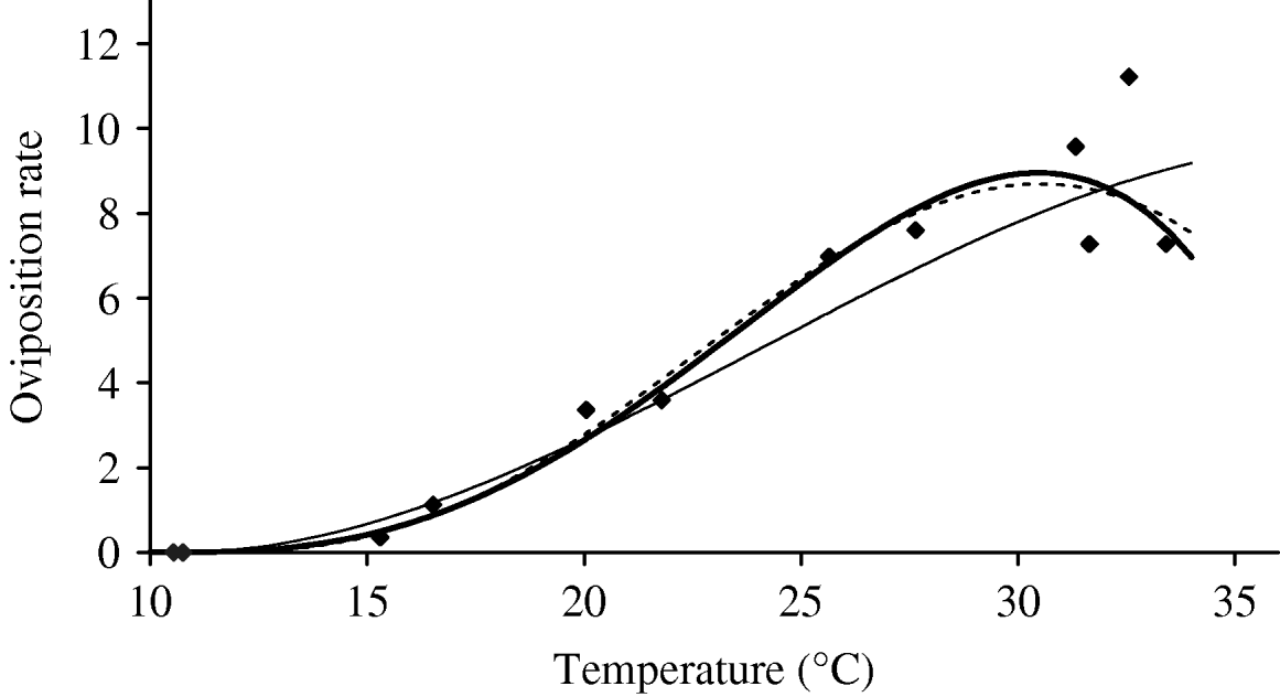
In the interval 15<T<30°C, Figure 3 shows a linearly increasing oviposition rate, while Figure 2 shows a slightly sloped line for the female mosquito mortality rate. Both figures present an interesting picture. In general the increase in ambient temperature is a beneficial factor for the maintenance of the vital physiological activities (e.g. maturation of fertilized eggs) of the mosquito. Figure 3 shows a quasi-linear increase in the oviposition rate with temperature, showing indirectly that the physiological activities increase in order to maturate fertilized eggs. Figure 2, in turn, shows a quasi-constant mortality rate with temperature. Joining both findings, we can conclude that a possible gain in the survival of female mosquitoes with temperature is counterbalanced by intense physiological activities, because in laboratory experiments all the conditions (especially food and bloodmeals) are favourable.
Let us now assume that the number of eggs laid by female mosquitoes could be considered as an indicator of biting activity in order to maturate the fertilized eggs. Then, from the above findings, we can conjecture that the female mosquitoes survive for the same periods of time in the interval 15<T<30°C, because an increase in biting frequency, in order to maturate more fertilized eggs, could increase physiological activities of female mosquitoes. Assuming that a female mosquito becomes infected during the bloodmeal – from that moment on the dengue virus infects increasing numbers of cells and drives all the cellular machinery to produce copies of them. This deviation of the cellular function can decrease the demand for maturation of fertilized eggs, which potentially could increase the lifespan of the infected mosquito without a decrease in biting activities.
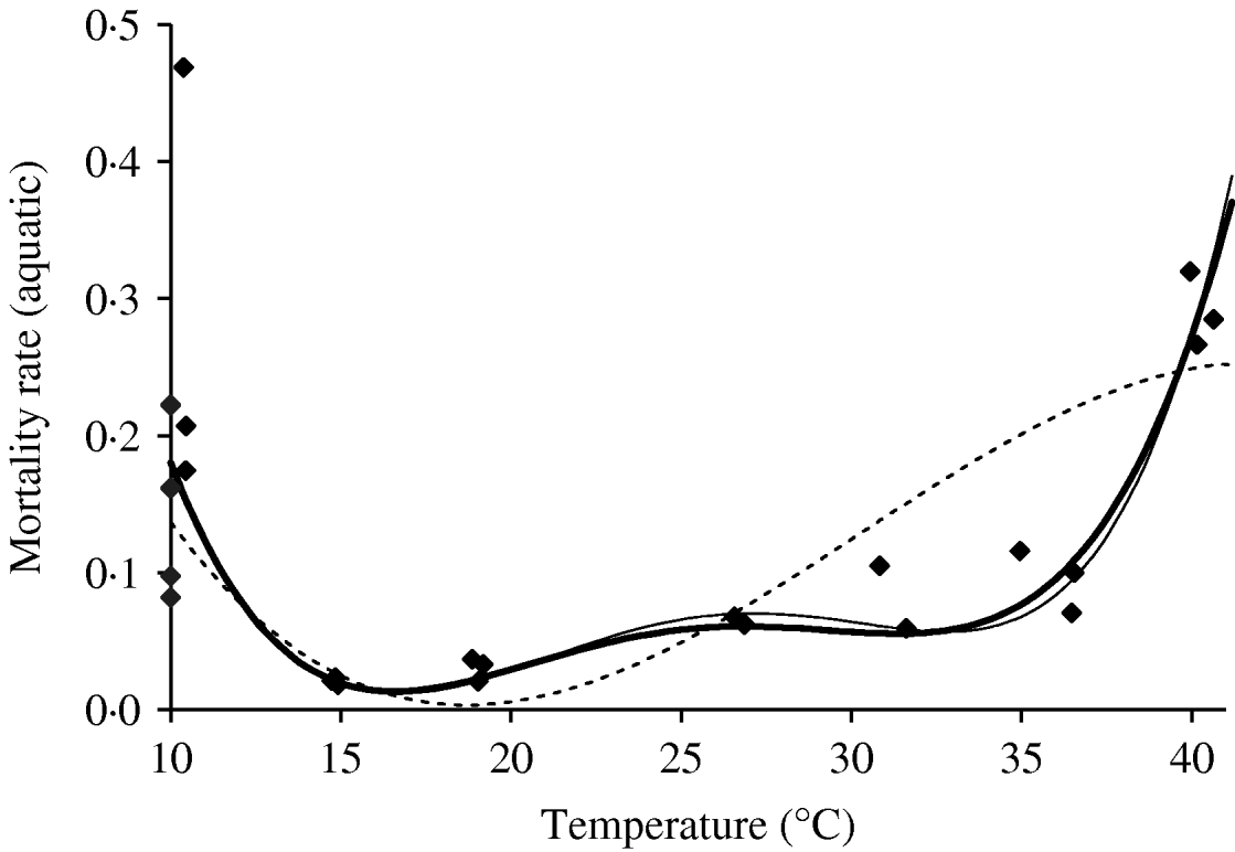
Based on Table 8 (Appendix B), we fit the mortality rate of the whole aquatic phase as a function of temperature. Figure 4 shows the temperature-dependent mortality rate of the whole aquatic phase. We observed behaviour similar to that found in the female mosquito mortality rate. We chose a fourth-degree polynomial for the survival study of the aquatic phase, as for adult mosquitoes.
The fitting of the aquatic phase mortality rate as a function of temperature. The estimated coefficients b i with errors in parentheses [days−1×(°C)–i] are: b 0=2·130 (5·260×10−2), b 1=−3·797×10−1 (1·043×10−2), b 2=2·457×10−2 (7·437×10−4), b 3=−6·778×10−4 (2·234×10−5) and b 4=6·794×10−6 (2·373×10−7) (–––). Fittings for the third- (- - -) and fifth- (–––) degree polynomials and the observed values (◆) are also shown.
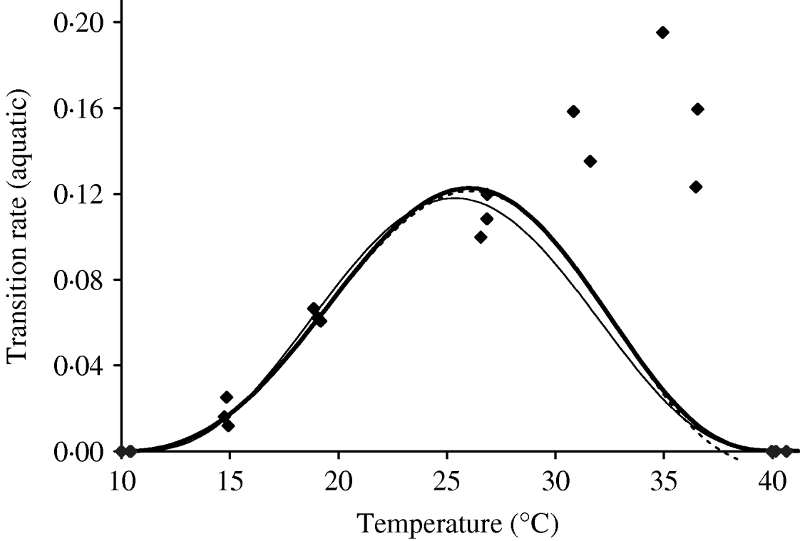
Based on Table 10 (Appendix B), we fit the transition rate of the whole aquatic phase as a function of temperature. We assume πq=0 and  as the temperatures at which aquatic forms do not develop into adult mosquitoes. Figure 5 shows the temperature-dependent transition rate of the whole aquatic phase. For 10·02<T<10·42°C, the negative values in the aquatic phase mortality rate must be changed to zero. We choose a seventh-degree polynomial for the transition study, which presents an abrupt decrease at higher temperatures, missing data around 30°C. One explanation for this poor fitting is due to the very small errors arbitrarily assigned to lower and higher temperatures. Another is the need for nonlinear fitting methods. A generalized additive model [Reference Hastie and Tibshirani9] can be used, considering, for instance, the transcendental function p(T)eq(t), where p(T) and q(T) are polynomials, similar to those used in [Reference Massad10].
The fitting of the aquatic phase transition rate as a function of temperature. The estimated coefficients b i with errors in parentheses [days−1×(°C)–i] are: b 0=1·310×10−1 (3·750×10−2), b 1=−5·723×10−2 (1·385×10−2), b 2=1·164×10−2 (2·073×10−3), b 3=−1·341×10−3 (1·628×10−4), b 4=8·723×10−5 (7·250×10−6), b 5=−3·017×10−6 (1·839×10−7), b 6=5·153×10−8 (2·471×10−9) and b 7=−3·420×10−10 and (1·365×10−11) (–––). Fittings for the sixth- (- - -) and eighth- (–––) degree polynomials and the observed values (◆) are also shown.
The main limitation factor to the persistence of the mosquito population lies in the aquatic form and in the production of eggs by female mosquitoes. Tables 5 and 10 (Appendix B) show that at lower temperatures there are neither the development of the immature forms to adults nor increases in oviposition (and the gonadotrophic cycle); however, at higher temperatures there is only the development of immature forms.
The entomological parameters shown in Figures 2–5 are a good example of the influence of the temperature in the size of the mosquito population. How can we extract useful information taking into account all parameters simultaneously? Population dynamics theory addresses this question.
ASSESSING THE EFFECTS OF TEMPERATURE ON THE SIZE OF THE MOSQUITO POPULATION
The ecological and epidemiological results obtained from the mathematical modelling presented earlier are now dealt with in regard to the entomological parameters estimated from temperature-controlled experiments described in the previous section.
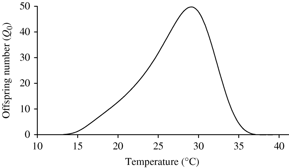
Figure 6 shows the curve of the basic offspring number Q 0, using equation (3). As shown in the ‘Modelling dynamics’ section, the mosquito population cannot be maintained in a geographic region if Q 0⩽1. From Figure 6, Q 0⩽1, if T<13·60°C and T>36·55°C, and in this temperature range there is no dengue transmission because the region is free from mosquitoes. When Q 0>1, which occurs in the temperature range 14<T<36°C, the number of the mosquitoes at steady state , from the second part of equation (2), is linearly proportional to the carrying capacity C, but for Q 0, the numbers of the mosquito population increases monotonically from 0, at Q 0=1, to the asymptote πqC/μf, when Q 0 is very great (Q 0→∞). We stress the fact that the range of higher risk of dengue outbreaks, taking into account only Q 0, is situated between 27 and 30°C. However, the incidence of dengue is dependent not only on the risk factor Q 0, but also on the available number of humans and mosquitoes susceptible to acquire the infection and the frequency of contacts among them.
The basic offspring number Q 0 as a function of temperature is shown, with k=0·5 and f=0·5. The model assumes one compartment comprising larval and pupal stages, and we have Q 0>1 for 13·60⩽T⩽36·55°C.
As shown in Appendix A, the absence of mosquito population is strongly robust when the average number of female offspring is <1, i.e. Q 0⩽1. This can partially explain what occurs in temperate regions: A. aegypti mosquitoes can eventually invade this region during hot and wet summer seasons; however, they are not able to colonize this region due to the low temperature in winter seasons. However, if the fitness of mosquitoes is increased by variations in the abiotic conditions, especially due to global warming, resulting in Q 0>1, then the invasion and colonization of this region by A. aegypti can be expected [Reference Ferreira, Yang and Esteva11].
We estimated the temperature-dependent entomological parameters φ, πq, μq and μf and, as a consequence, these parameters vary with calendar time. However, in the present study we have taken into account the annual mean values and assessed the effect of the temperature on the basic offspring number Q 0. By performing this kind of study, our aim was the assessment of the increasing trend in temperature, for instance due to global warming, in mosquito colonization and the consequent dengue outbreak in regions of low temperature believed to be safe from dengue disease. For this reason, we ignored the annual variation of the entomological parameters, which is an issue for a future work.
DISCUSSION AND CONCLUSION
We developed a mathematical model to assess the effects of temperature on the size of the A. aegypti mosquito population. In order to give the modelling realistic values with regard to the model parameters, temperature-controlled experiments were performed with the aim of studying the influence of temperature on the mortality and transition rates in the life-cycle of the mosquito. The temperature-dependent entomological parameters were determined for mosquitoes found in the city of Marìlia, São Paulo State, Brazil. Parametrized probability functions used to fit follow-up data showed some advantages. Even in extreme temperatures at which very low numbers of individuals suffered a change of state (from live to death in different stages of life-cycle and transition from one stage to another in the aquatic phase), the adjusted probability functions provided reasonable estimations for parameters.
From the point of view of the A. aegypti entomology, the temperature-dependent parameters can be used to address many questions concerning mosquito's life-cycle. For instance, the optimal range of temperature for survival of the adult mosquitoes is 15<T<30°C, while for the aquatic stages, we have 15<T<35°C. However, the temperature at which quick transitions occur in the aquatic stages is around 26°C. Therefore, the effect of temperature is distinct in different stages of the mosquito's life-cycle [Reference Focks12, Reference Focks13]. At low temperature (10°C), we found that (a) an increase of 0·38°C allowed the transition from L1 to L2 and, (b) pupal stage is the most resistant aquatic form, followed by L4 and L3. At high temperature (40°C) the aquatic phase is restricted to the larval stage, none of which reach the pupal stage.
We have several entomological parameters that present different behaviours concerning temperature. The survival of the aquatic and adult forms is U-shaped, given, respectively, by the ranges 15<T<35°C and 15<T<30°C. The rate at which female mosquitoes lay eggs increases quasi-linearly, and the transition rate between successive stages is bell-shaped, with the maximum at 26°C. To encompass the different influences of temperature in the entomological parameters, we applied population dynamics theory to assess the time evolution of the mosquito population. The mathematical model we proposed yielded the basic offspring number Q 0. This number increases up to 29°C, and then decreases quickly. In the range 13·60⩽T⩽36·55°C, we have Q 0>1, i.e. the mosquito population persists in the human population. The optimal temperature to produce the highest number of offspring is 29·2°C.
The temperature-dependent basic offspring number Q 0 is a key parameter to assess both the effects of global-warming and vector-controlling efforts. Regarding global warming, the basic offspring number increases monotonically until 29°C increasing the risk of dengue disease in subtropical regions. Another consequence is an increase in the expectation (probability) of invasion and colonization by A. aegypti mosquitoes in temperate regions. Hence global warming should be seriously considered by public health authorities because both regions are heavily populated. By restricting only the variation of temperature, the gains with global warming seem very restrictive, since the temperature at which the mosquito population is naturally eradicated must be higher than 36°C.
The modern lifestyle produces as residuals recipients that are appropriate to receive eggs from female mosquitoes. This is one of the reasons that explains the re-emergence of A. aegypti mosquitoes in heavily populated areas and also their resistance when faced with eradication measures. To eradicate the dengue vector, chemical and mechanical controls are applied to the mosquito population. The chemical control measure can be incorporated in the model introducing additional mortality rates in the larval and pupal stages and in adult mosquitoes. One effect is the reduction in the basic offspring number, according to equation (3). Mechanical control does not affect the basic offspring number, but does reduce the total number of breeding sites, decreasing the carrying capacity according to the second part of equation (2). However, this form of control needs an active adherence of the individuals to maintain the reduced breeding sites, in order to avoid a quick return to the previous infestation level [Reference Kroeger14]. Therefore, the basic offspring number, in conjunction with the past incidence of dengue infection, should be a very useful tool to help in designing and implementing the controlling mechanisms to diminish the population size of mosquitoes by public health authorities.
Finally, in the present study we dealt with entomological values varying with temperature, and assessed the mosquito population size. In a companion paper [Reference Yang15], the effects of temperature on dengue transmission are analysed.
APPENDIX A
Steady state
We show that if Q 0<1, then the trivial equilibrium point is stable; otherwise, the non-trivial equilibrium point is stable. We take this number as the sentinel for dengue outbreak, due to: (1) this number is related to the size of the mosquito population, and (2) the greater this number, the more effort that must be spent to eliminate the mosquito population.
A steady state is called locally stable if small displacements from the equilibrium value return to the steady state. Mathematically this idea consists in calculating the roots of the characteristic equation Λ(λ) defined as

where det stands for the determinant of a matrix, J* is the Jacobian matrix, which is the linearization of the system of equation (1) at the equilibrium point, given by
![J \ast \equals \left[ {\matrix{ { \minus kf\phi \displaystyle{{\bar{M}} \over C} \minus \lpar \pi _{q} \plus \mu _{q} \rpar } \tab {kf\phi \left( {1 \minus \displaystyle{{\bar{A}} \over C}} \right)} \cr \hskip20pt {\pi _{q} } \tab { \minus \mu _{f} } \cr} } \right] \comma](https://static.cambridge.org/binary/version/id/urn:cambridge.org:id:binary:20160921000207967-0817:S0950268809002040:S0950268809002040_eqnU5.gif?pub-status=live)
and I is a 2×2 identity matrix.
The characteristic equation corresponding to the trivial equilibrium point, substituting Ā=0 and =0 in the matrix J*, is

where the coefficients are
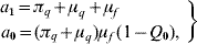
with the basic offspring number Q 0 being given by equation (3). This second-degree polynomial has the following property: if a 1>0 (this is always true) and a 0>0, then the roots of the polynomial (eigenvalues) are negative numbers (if real number), or have a negative real part (if imaginary numbers). Both conditions are known as the Routh–Hurwitz criteria for second-degree polynomials [Reference Edelstein-Keshet16]. Note that a 0>0 when Q 0<1, and the trivial equilibrium point is locally asymptotically stable for Q 0<1; otherwise, it is classified as unstable.
Another analysis for the trivial equilibrium is global stability. While local stability is related to the return to the trivial equilibrium point for small perturbations, global stability states that all trajectories go to the trivial equilibrium point for all amplitudes of displacement. To prove that the absence of a mosquito population is globally stable for Q 0⩽1, we use the function V:R +2→R given by
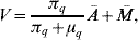
whose orbital derivative is
![\dot{V} \equals \minus \mu _{f} \left[ {{{Q_{\setnum{0}} \bar{A}} \over C} \plus \lpar 1 \minus Q_{\setnum{0}} \rpar } \right]\bar{M}.](https://static.cambridge.org/binary/version/id/urn:cambridge.org:id:binary:20160921000207967-0817:S0950268809002040:S0950268809002040_eqnU7.gif?pub-status=live)
The La Salle–Lyapunov theorem [Reference Hale17] establishes that for V>0, if we have  , then the equilibrium point is globally stable. We observe that
  for Q 0<1, and for Q 0=1 we have
  if =0 or Ā=0. By inspecting equation (1), it can be seen that the maximal invariant set contained in is the trivial equilibrium point. Then, the trivial equilibrium point is globally asymptotically stable for Q 0⩽1.
The importance of global stability for the trivial equilibrium point relies on the fact that if eradication of the mosquito population is achieved (Q 0⩽1), then the absence of mosquitoes is strongly robust. Even the introduction of a great amount of mosquitoes is not able to result in recolonization.
The next result states that if Q 0>1, then the steady-state situation is infestation by the mosquito population. The characteristic equation corresponding to the non-trivial equilibrium point, substituting

in the matrix J*, is

where the coefficients are
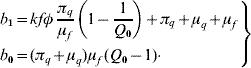
This second-degree polynomial obeys the Routh–Hurwitz criteria, b 1>0 (always true) and b 0>0 (when Q 0>1). Hence, the non-trivial equilibrium point is locally asymptotically stable if Q 0>1; otherwise, unstable.
To summarize, when Q 0⩽1, there is only the trivial equilibrium point, and the absence of mosquitoes is strongly robust. When Q 0>1, the trivial equilibrium is unstable, and infestation by mosquitoes becomes the stable situation. In other words, any small introduction of mosquitoes in a region previously free of them results in the (re-)colonization, and the level of infestation is given by the basic offspring number Q 0.
APPENDIX B
Estimation of the follow-up data
As we have pointed out in the main text, the temperature (humidity can not be controlled) inside the germination chamber was adjusted to simulate the seasonal photoperiod that naturally occurs for different temperatures. However, the adopted temperature was the weighted mean calculated from the records of the thermohygrograph situated inside the chamber. The average relative humidity (standard deviation) was also calculated from the thermohygrograph records for different temperatures (°C): 73·71 (3·15), 74·31 (3·74), 76·20 (3·95), 76·13 (1·87), 76·11 (2·14) and 69·31 (8·17), respectively, for 10, 15, 20, 25, 30 and 35°C. The relative humidity in all temperatures was around 75%.
The temperature-controlled experiments with adult mosquitoes were to determine the temperature-dependent mortality rate. In this study a very large number of eggs are driven to hatch and emerge as adult mosquitoes simultaneously. The first emerging male and female mosquitoes are captured and placed in a cage for follow-up.
Female mosquitoes are responsible for dengue virus transmission in humans, leaving the male mosquito with only indirect participation. To mature the fertilized eggs after coupling, females need human blood. The cage containing mosquitoes was handled every day to remove dead mosquitoes and the oviposition traps, during which time some mosquitoes could escape, even during this short period. For this reason we counted all mosquitoes in the cage each day. When some mosquitoes escaped, the number was recorded in the day just before the current observation day, and was treated as censored data. The lost mosquitoes are a source of error measurement, and contribute to increased survival time.
Tables 2 and 3 present the parameters τ and β fitted against the follow-up data corresponding to male and female mosquitoes, respectively. Note that male and female mosquitoes are placed together in a cage.
Estimated values of the half age τ (and variance στ2) and heterogeneity β (and variance σβ2) for male mosquitoes
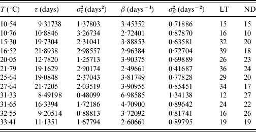
The maximum or last time (LT in days) of observation and the number of dead mosquitoes (ND) are shown. The sample size for each follow-up is 30, except for the temperatures 21·79 and 32·55°C, which are, respectively, 33 and 31. One mosquito was still alive on the last day of observation for the temperatures 21·79 and 27·64°C.
Estimated values of the half age τ (and variance στ2) and heterogeneity β (and variance σβ2) for female mosquitoes
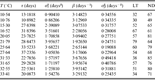
The maximum or last time (LT in days) of observation and the number of dead mosquitoes (ND) are shown. The sample size for each follow-up is 100, except for the temperature 10·76°C, which is 89. One mosquito was still alive on the last day of observation for the temperatures 15·30 and 27·64°C.
The fitted heterogeneity degree β appears as a high value and seems to present a weak dependence with the temperature and gender: at high temperature they behave slightly more homogeneously, and females are slightly more heterogeneous than males. Conversely the half-time τ shows clear dependency with temperature and gender: the optimal temperature for the survival of mosquitoes is around 25°C and females survive more than males. Let us focus on two extreme fittings. The highest fitted value of β is in Table 2 corresponding to 31·33°C. As shown in Figure 1, the higher the heterogeneity degree, the more homogeneously the mosquitoes behave. At this temperature the followed-up male mosquitoes died around the estimated half age τ and, as a consequence, presented the lowest error στ2. However, the lowest value of β is in Table 3 corresponding to 21·79°C. As shown in Figure 1, the lower the heterogeneity degree, the more heterogeneously the mosquitoes behave. At this temperature the followed-up female mosquitoes died very dispersed in regard to the estimated half age τ and, as a consequence, presented the highest error στ2.
In the modelling we did not take into account mating among mosquitoes. For this reason we restricted our estimations to only female mosquitoes. The average survival time η and its error ση are calculated using equations (6) and (7) with τ and β given in Table 3. From these values we calculate the mortality rate μ and its error σμ using equations (8) and (9). Table 4 gives the average survival time and the mortality rate of the female mosquitoes.
Calculation of the average survival time η (and error ση) and the mortality rate μ (and error σμ) for female mosquitoes
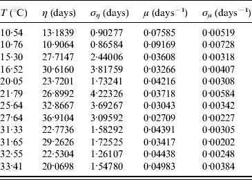
We observed that the main contribution to the uncertainty (error) in the mortality rate is the heterogeneity degree parameter.
In the experiments involving adult mosquitoes the number of eggs laid by females was also recorded. Table 5 presents the mean number of eggs per day per female and the first day at which eggs were found in the cage.
Calculated values of the average number of oviposition rate φ and the first day (FD in days) of oviposition
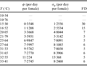
Female mosquitoes did not lay eggs at temperatures of 10·54 and 10·76°C.
Excluding 31·33°C, for all other temperatures the error obtained from the data is greater than the mean value, showing that oviposition is very heterogeneous in female mosquitoes. At almost 10°C no eggs were laid, and at 15·30°C the first oviposition occurred after 30 days of observation (or, female mosquitoes reaching age 30 days). At this temperature the mean survival time was 27·7 days. Interestingly, a temperature increase of 1·22°C reduced the first day of oviposition by half, and an additional reduction by half is observed at 20·05°C. Above this temperature the first oviposition occurred between days 5 and 6 days of observation. Remembering that the successive times of observation differ by 1 day, the first oviposition occurred between ages 4 and 5 days. The lower bound (4 days) of delay for females to lay eggs seems reasonable if we take into account the gonadotrophic cycle, the time needed to mature the fertilized eggs (around 3 days after bloodmeal), and the fact that the females are able to copulate 24 h after the emerging.
The temperature-controlled experiments in the aquatic phase of mosquitoes were aimed at the determination of temperature-dependent mortality and transition rates. In this study a large number of eggs are driven to hatch simultaneously to larval stage. Of these, around 100 larvae, except for three experiments where around 50 larvae were chosen, are selected and these are then followed up. At the corresponding day of observation, the numbers of (a) deaths in larval and pupal stages and (b) emerging pupae and adult mosquitoes are recorded. Table 6 gives the summary of the follow-up of the aquatic phase. Based on this, the mortality and transition rates are estimated.
Number of the followed-up individuals (NF), the maximum or last time (LT in days) of observation, the numbers of dead larvae before reaching pupal stage (NDL) and dead pupae before emerging as mosquitoes (NDP)
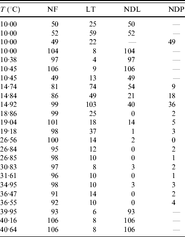
At low temperature (rows 4–6 in Table 6), the hatched eggs did not develop to pupae, but all died at the larval stage. At 10°C, all larvae died in the first larval stage (instar), but at 10·38°C and 10·45°C, we observed development up to second instar (L1–L2, none of which reached L3). For this reason, we performed additional experiments in which follow-up was begun at different instars of larval stage: the procedure was hearing the larvae at an optimal temperature (25°C) and then exposing L2, L3, L4 and pupae at 10°C. In the follow-up of the second (L2) and third (L3) instars, corresponding to rows 7 and 1, respectively, in Table 6, the larvae developed to the next instar (L2–L3 and L3–L4, respectively). However, when we began the follow-up in the fourth (L4) instar and pupae, all larvae and pupae died, which correspond to rows 2 and 3, respectively, in Table 6.
Table 7 shows the parameters τ and β fitted against the follow-up data corresponding to the survival of the whole aquatic phase.
Estimated values of the half age τ (and variance στ2) and heterogeneity β (and variance σβ2) for the survival of the whole aquatic phase
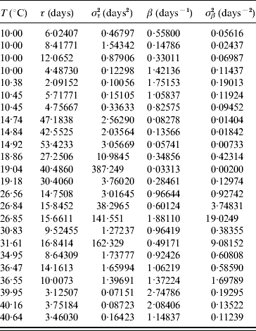
Estimated parameters measuring the time from eggs hatching until emergence of adult mosquitoes (all followed-up larvae died for T⩽10·45°C and T⩾39·95°C, for which reason these estimated parameters correspond to the larval stage).
At low (10°C) and high (40°C) temperatures all larvae died [18]. At low temperatures larvae survived more often than at high temperatures, but they behaved more heterogeneously. We now explain the fitting where τ<στ2 or β<σβ2, which occurred at 18·86, 19·04, 26·84, 26·85, 31·61 and 36·55°C. The deaths at 18·86 and 36·55°C (four) occurred exactly at 15 and 8 days of observation, respectively, at 19·04, 26·84 and 31·61°C all deaths occurred before the occurrence of the first transition to pupal stage and at 26·85°C a single death occurred during the last day of observation. Finally, the two deaths that occurred at 36·47°C illustrate the opposite case τ>στ2 or β>σβ2: they occurred at two different days (days 10 and 14 of observation).
The survival study is determined by the number of deaths occurring during follow-up. The aquatic phase of the mosquito comprises larval and pupal stages, which the hatched eggs must pass through in order to emerge in the adult form. Death is an incidental occurrence, for this reason in favourable temperatures we face an anomalous fitting due to absence or reduced number of deaths, and also due to the occurrence of larvae and pupae dying on the same observation day.
The average survival time η and its error ση are calculated using equations (6) and (7) with τ and β given in Table 7. From these values we calculate the mortality rate μ and its error σμ using equations (8) and (9). Table 8 gives the average survival time and the mortality rate of the whole aquatic phase.
Calculated values of the average survival time η (and error ση) and the mortality rate μ (and error σμ) for the whole aquatic phase
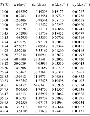
In the aquatic phase, besides survival in the larval and pupal stages, each aquatic form must successfully be transformed in the sequence egg–larva–pupa to emerge as an adult form in order to perpetuate its species. In Table 9 we present the parameters τ and β fitted against the follow-up data corresponding to the transition of the whole aquatic phase.
Estimated values of the half age τ (and variance στ2) and heterogeneity β (and variance σβ2) for the transition of the whole aquatic phase
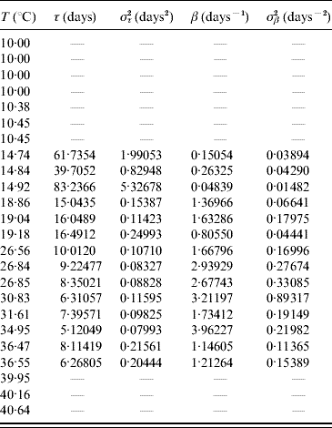
Estimated parameters measure the time from eggs hatching until emergence of adult mosquitoes.
The larvae and pupae behaved heterogeneously at low temperature, and at 14·92°C the most heterogeneous behaviour was observed. At temperatures >20°C the behaviour was more homogeneous, especially between 26 and 35°C. The heterogeneous behaviour outside the optimal temperature seems to be an attempt to compensate for the adverse environment which results in a high mortality rate (Table 8).
The average transition time ξ and its error σξ are calculated using equations (6) and (7) with τ and β given in Table 9. From these values we calculated the transition rate π and its error σπ using equations (8) and (9). Table 10 presents the average transition time and the transition rate of the whole aquatic phase.
Calculated values of the average transition time ξ (and error σξ) and the transition rate π (and error σπ) for the whole aquatic phase
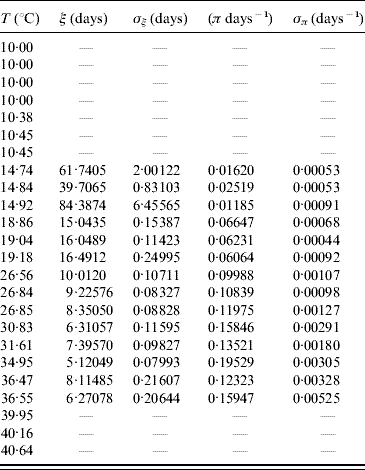
In lower (T⩽10·45°C) and higher (T⩾39·95°C) temperatures we did not observe the transition of hatched eggs to adult forms.
ACKNOWLEDGEMENTS
This work was supported by grant from FAPESP (Polìticas Públicas and Temático). H.M.Y. thanks the CNPq for the award of a fellowship. The authors are grateful for the comments and suggestions provided by anonymous referees, which contributed to the improvement of this paper.
DECLARATION OF INTEREST
None.



