


Introduction
Heirs’ property, land passed down to family members without a clear legal title, typically arises when the property owner dies intestate. In these cases, heirs receive an undivided interest in the property, holding it as “tenancy-in-common.”Footnote 1 Because estates are often not probated, the legal title becomes fragmented across generations, resulting in unclear ownership rights among multiple co-owners (Pierce, Reference Pierce1973). Despite its longstanding presence, heirs’ property remains a critical yet underexplored issue in the United States. This phenomenon is deeply rooted in historical, legal, and cultural contexts (Dyer and Bailey Reference Dyer and Bailey2008; Mitchell Reference Mitchell2001, Reference Mitchell2016; Johnson Gaither Reference Johnson Gaither2016) and poses significant challenges to land use, community economic development, and broader societal equity (Johnson Gaither and Zarnoch Reference Johnson Gaither and Zarnoch2017).
Heirs’ property has two major challenges: economic inefficiency and the threat of displacement, due to its characteristics for heirs, the absence of clear title and the complexities of tenants-in-common (Deaton et al. Reference Deaton, Baxter and Bratt2009; Dyer and Bailey Reference Dyer and Bailey2008). First, lacking a clear title hinders heirs from proving ownership. Consequently, heirs are restricted in their access to financial tools such as home mortgages, commercial loans, and government programs. These include the United States Department of Agriculture’s (USDA) farm loans and payment programs–such as commodity payments and subsidized crop insurance–and the Federal Emergency Management Agency’s (FEMA) disaster assistance and recovery programs (Deaton Reference Deaton2005, Reference Deaton2012; Dyer et al. Reference Dyer, Bailey and Tran2009; Johnson Gaither et al. Reference Johnson Gaither, Carpenter, McCurty, Toering, Johnson Gaither, Carpenter, McCurty and Toering2019; Raker and Woods Reference Raker and Woods2023; Winters-Michaud et al. Reference Winters-Michaud, Burnett, Callahan, Keller, Williams and Harakat2024). Without formal titles or clear legal documentation, heirs face considerable challenges in meeting the eligibility requirements for these programs, thereby exacerbating barriers to financial and disaster recovery support. Second, tenancy-in-common is an unstable form of ownership, complicating property management (Deaton Reference Deaton2007; Johnson Gaither Reference Johnson Gaither2016). It requires agreement among all heirs for any commercial land use, such as timber sales, development, or leasing, which often results in the land remaining underdeveloped. Many studies have also highlighted that this form of ownership is significantly linked to land loss among African Americans (Dyer et al. Reference Dyer, Bailey and Tran2009; Mitchell Reference Mitchell2001). These conditions of heirs’ property not only hinder productive land use as leverage but also limit the potential for income generation and wealth transfer across generations (Deaton Reference Deaton2012).
The adverse effects of heirs’ property extend beyond individuals to communities. The consistent limitation of properties to generate income and build wealth contributes to persistent poverty in underserved populations and rural areas. Heirs’ property is more prevalent among historically underserved groups, including African Americans in the rural South, Hispanics in the Southwest, Whites in Appalachia, and Native Americans in former reservation areas, and possibly among Hispanic colonia residents near the U.S.–Mexico border regions (Bailey et al. Reference Bailey, Zabawa, Dyer, Barlow, Baharanyi, Johnson Gaither, Carpenter, McCurty and Toering2019; Deaton Reference Deaton2007, Reference Deaton2012; Dobbs and Johnson Gaither Reference Dobbs and Johnson Gaither2023; Johnson Gaither et al. Reference Johnson Gaither, Carpenter, McCurty, Toering, Johnson Gaither, Carpenter, McCurty and Toering2019; Pippin et al. Reference Pippin, Jones and Johnson Gaither2017; Winters-Michaud et al. Reference Winters-Michaud, Burnett, Callahan, Keller, Williams and Harakat2024). These issues associated with heirs’ property perpetuate racial and social inequities while also constraining economic development and growth in rural communities. The consequences of heirs’ property are widely acknowledged, particularly in how it restricts the intergenerational transfer and accumulation of wealth across a broad spectrum of populations, including impoverished, marginalized, middle- and working-class communities.
The spatial distribution of heirs’ property is not random. It is spatially concentrated in the southern U.S. and is mutually influenced by historical land allocation practices, demographic and socioeconomic factors, and related policies. Therefore, it is crucial to understand where the spatial clusters of heirs’ property exist and what factors are associated with them. Such knowledge is a first step in outreach and education and developing targeted interventions to resolve title issues, promote land management and economic development, and protect vulnerable populations from land loss.
Researchers, for decades, have sought to address the scale and location of heirs’ property since the early studies of Graber (Reference Graber1978) and the Emergency Land Fund (1980). However, due to a lack of available data, questions have remained unanswered despite a consensus that the extent and location of heirs’ property should be studied. Most research has focused on single counties (e.g., Deaton, Reference Deaton2005, Reference Deaton2007; Dyer et al. Reference Dyer, Bailey and Tran2009) or multiple communities rather than the entire country. Dobbs and Johnson Gaither (Reference Dobbs and Johnson Gaither2023) recently estimated heirs’ property for over 3,000 counties using parcel data from Lightbox Holdings.Footnote 2 The increased availability of such data has facilitated large-scale research on heirs’ property, as demonstrated by the works of Dobbs and Johnson Gaither (Reference Dobbs and Johnson Gaither2023), Moodie et al. (Reference Moodie, Wiley and George2023), and Thomson and Bailey (Reference Thomson and Bailey2023), who measured the extent and market value of heirs’ property.
Our analysis explores the socioeconomic and demographic characteristics of counties with high concentrations of heirs’ property, examining variables such as population, urban-rural locations, and economic and financial status. This approach highlights factors significantly associated with the presence of heirs’ property, providing insights into the compounded vulnerabilities of this phenomenon. Furthermore, we examine neighboring effects to understand whether and how the spatial clusters of heirs’ property impact (or are impacted by) surrounding areas. This aspect of our research sheds light on the broader implications of heirs’ property for regional development, land use planning, and social equity. By examining the interconnections between heirs’ property clusters and their broader socioeconomic context, this study provides a deeper understanding of the challenges and opportunities associated with this unique form of land ownership.
This article makes a novel contribution to the literature by mapping spatial clusters of heirs’ property, identifying the socioeconomic factors associated with these clusters, and examining the presence of neighboring effects through empirical analysis. While previous studies, such as Dobbs and Johnson Gaither (Reference Dobbs and Johnson Gaither2023), conducted spatial analyses of heirs’ property, including a binary local indicators of spatial association (LISA) analysis of heirs’ property and FEMA’s National Risk Index (NRI) in North Carolina, this study builds on their findings by extending the analysis to a national scale. Specifically, we examine spatial variation in the prevalence of heirs’ property using county-level data across the contiguous United States. We employ both spatial descriptive analysis tools to demonstrate the spatial clustering of heirs’ property and spatial econometric models to evaluate the impact of socioeconomic and spatial factors on the prevalence of heirs’ property. To our knowledge, this is the first study to analyze socioeconomic and demographic factors from a spatial perspective across counties in the contiguous U.S. and their relationship to heirs’ property distributions. Through this analysis, we aim to provide policy makers, researchers, and practitioners with valuable insights into addressing the complexities of heirs’ property and fostering more equitable and sustainable land use practices.
Literature review and background
Over the decades, scholars have documented heirs’ property studies at various scales and perspectives, contributing to a growing body of knowledge about its extent, economic implications, and the socioeconomic factors influencing its prevalence. The first significant strand of research has focused on assessing the extent of heirs’ property and its economic value. Early studies, prior to the national-level estimation by Dobbs and Johnson Gaither (Reference Dobbs and Johnson Gaither2023), largely relied on more localized methodologies, such as tax and court record reviews, surveys, and field data collection (Deaton Reference Deaton2005; Dyer et al. Reference Dyer, Bailey and Tran2009; Georgia Appleseed 2013; Graber Reference Graber1978). These studies provided foundational insights but were often limited to single communities/counties or small regions.
Graber (Reference Graber1978) conducted one of the earliest investigations, estimating that about one-third of rural Black-owned land in five southern states (Alabama, Georgia, Mississippi, North Carolina, and South Carolina) qualified as heirs’ property. This finding was based on a detailed review of county tax rolls and information from local tax auditors in ten counties in those states. Deaton (Reference Deaton2005) analyzed tenancy-in-common ownership through a phone survey of a random sample of property owners in Letcher County, Kentucky. This study revealed that approximately 24 percent of respondents reported owning heirs’ property or similar landholding arrangements, underscoring the prevalence of this issue even in rural Appalachia. Building on this localized research, Dyer et al. (Reference Dyer, Bailey and Tran2009) focused on Macon County, Alabama, using 2007 property tax records to identify 1,512 heirs’ property parcels, which accounted for 4.1 percent of the county’s land area and were collectively valued at more than $25 million. The Georgia Appleseed (2013) report employed a two-stage process using online tax parcel data and real estate attorneys’ consultations to identify heirs’ parcels in five Georgia counties. This study uncovered 1,620 heirs’ parcels spanning 5,215 acres, with a total value of $58 million. Johnson Gaither and Zarnoch (Reference Johnson Gaither and Zarnoch2017) later summarized additional studies that estimated the extent of heirs’ property in the U.S. South (See Table 1 of their paper).
As research progressed, scholars began exploring the spatial dimensions of heirs’ property. Pippin et al. Reference Pippin, Jones and Johnson Gaither2017) were among the first to document the spatial distribution of heirs’ property across a broader geographic range, including ten counties in Georgia, Anderson County in South Carolina, and Cameron County in Texas. Using extensive data collection and indirect indicators, they estimated “potential heirs’ properties” accounted for 11%–25% of all parcels in ten Georgian counties studied, with a total appraised value of $2.1 billion. Similarly, heirs’ property represented 9% and 25% of total parcels in Anderson and Cameron Counties, valued at $821 million and $2.5 billion, respectively. These findings emphasized the need for more robust geographic analyses and the inclusion of spatial data to better capture the regional patterns of heirs’ property prevalence.
Recent advancements in data digitization and geospatial technologies have facilitated large-scale research on heirs’ property. Dobbs and Johnson Gaither (Reference Dobbs and Johnson Gaither2023) conducted a study using parcel-level data from LightBox to identify heirs’ property for all counties and census tracts in the U.S. Their analysis, based on 2021 data, estimated 444,172 heirs’ parcels, covering 9.2 million acres, with a total market value of $41.3 billion. Similarly, Thomson and Bailey (Reference Thomson and Bailey2023) analyzed property tax records across eleven southern states, estimating 496,994 heirs’ property parcels spanning 5.3 million acres, with a total market value of $41.9 billion. Building on these approaches, Moodie et al. (Reference Moodie, Wiley and George2023) analyzed 2022 county tax-assessment data provided by Fannie Mae via ICE Mortgage Technology, Inc., and estimated 508,371 parcels of heirs’ residential property across 44 states and Washington, D.C., with an assessed total value of approximately $32.3 billion. These studies mark a significant shift toward comprehensive geographic and economic assessments of heirs’ property, providing data to inform future research and policy efforts.
The second strand of heirs’ property research investigates the socioeconomic and geographical factors associated with its prevalence. Researchers generally agree that heirs’ property is more common in rural areas with economies reliant on agriculture, high poverty rates (or low income), and lower levels of educational attainment (Deaton Reference Deaton2005; Mitchell Reference Mitchell2001; Pippin et al. Reference Pippin, Jones and Johnson Gaither2017). For example, Deaton (Reference Deaton2005) hypothesized that the persistence of heirs’ property in rural Appalachia could be linked to socioeconomic conditions that limit access to legal and financial resources. However, exceptions exist. Dyer et al. (Reference Dyer, Bailey and Tran2009) found that in Macon County, Alabama, heirs’ property was prevalent even in incorporated areas. More recently, Kohanowski (Reference Kohanowski, Mitchell and Powers2022) highlighted the challenges of heirs’ property in major urban centers, broadening the focus beyond rural contexts. These studies suggest that while certain patterns exist – such as the association of heirs’ property with rural, low-income, and less-educated communities – heirs’ property remains a multifaceted issue influenced by diverse socioeconomic and geographic factors. However, empirical studies examining these factors on a broader scale remain limited.
Johnson Gaither and Zarnoch (Reference Johnson Gaither and Zarnoch2017) conducted one of the few empirical studies in this area, analyzing heirs’ property at the census block group level in Macon-Bibb County, Georgia. Their findings indicated that higher proportions of the Black population, lower education levels, and higher population density were associated with greater heirs’ property prevalence, while the poverty rate was not statistically significant in their analysis. These findings highlight the need for more comprehensive empirical analyses across the entire U.S. that examine the relationship between socioeconomic/demographic factors and heirs’ property prevalence. This study aims to fill that gap by providing empirical evidence from a spatial perspective.
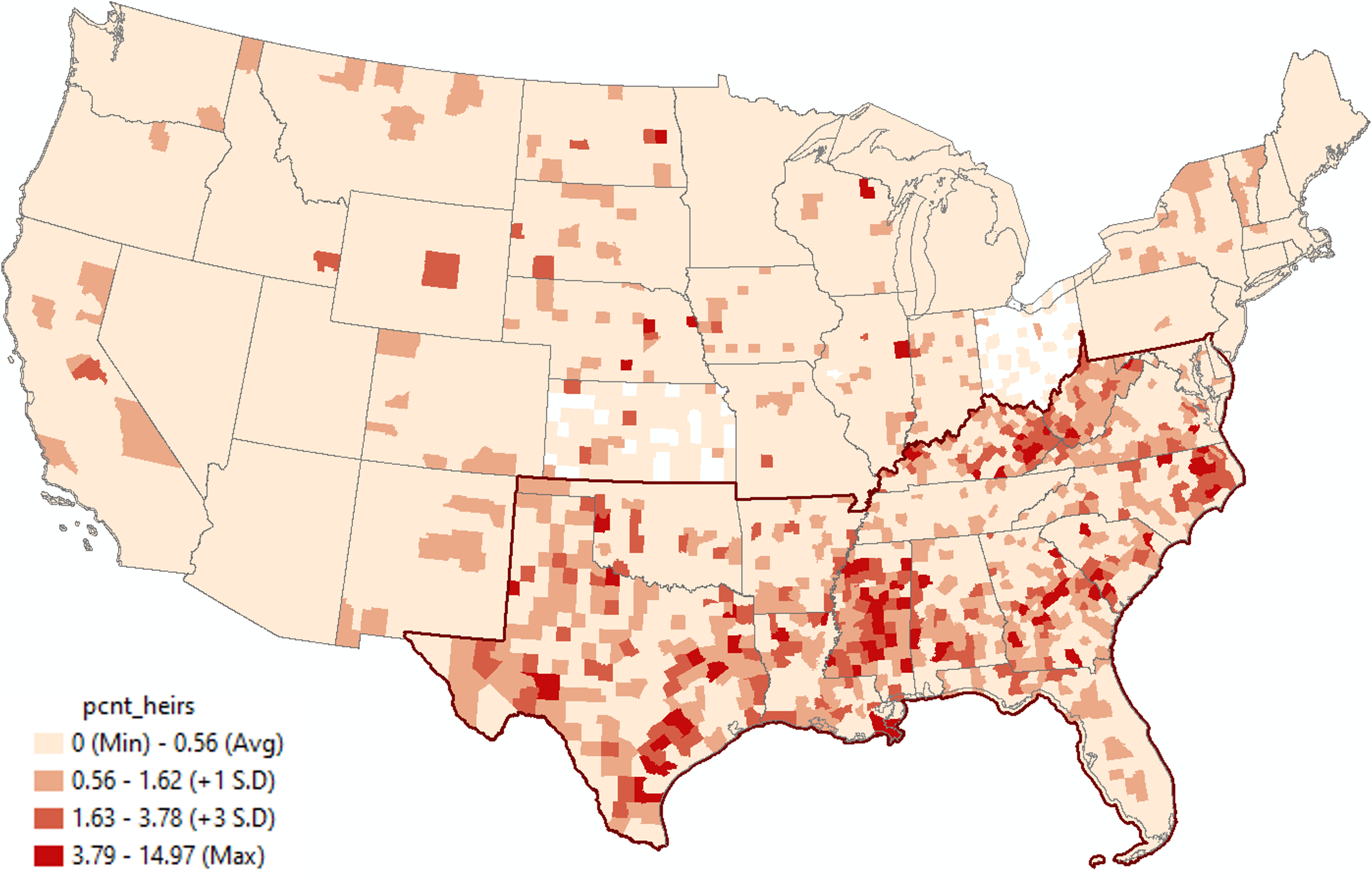
This study addresses these gaps by conducting a county-level analysis of heirs’ property prevalence within the contiguous U.S. To our knowledge, this is the first to examine correlations between socioeconomic and demographic factors and heirs’ property prevalence while incorporating spatial econometric models to account for spatial dependence. Figure 1 illustrates the geographic distribution of heirs’ property parcels, revealing significant clustering in the southern United States, with some exceptions in other regions. This pattern aligns with prior research identifying heirs’ property concentrations in specific populations or communities. Notably, counties with higher heirs’ property prevalence are often found within African American communities in the South, White communities in Appalachia, Latinx communities in the Southwest, and Native American communities on former reservations in the Great Plains and Western states (Deaton Reference Deaton2007, Reference Deaton2012; Dobbs and Johnson Gaither Reference Dobbs and Johnson Gaither2023; Winters-Michaud et al. Winters-Michaud et al. Reference Winters-Michaud, Burnett, Callahan, Keller, Williams and Harakat2024).
Spatial distribution of heirs’ property prevalence rate. Data source: Dobbs and Johnson Gaither (Reference Dobbs and Johnson Gaither2023). Note: Mean: 0.56% of total parcels, Median 0.17%, Standard Deviation (SD) 1.06%, Minimum 0%, and Maximum 14.97%; Empty counties have no data available; The red boundary presents the U.S. Census’s South Region.
Building on these studies, Dobbs and Johnson Gaither (Reference Dobbs and Johnson Gaither2023) employed LISA to identify hot spots of high heirs’ property prevalence. Their analysis revealed significant correlations between these clusters and social vulnerability metrics, such as FEMA’s NRI in North Carolina. Expanding on these findings, our study goes beyond spatial autocorrelation to explicitly analyze spatial dependence, exploring how the prevalence of heirs’ property in one county influences and is influenced by neighboring counties.
Method and data
Spatial dependence and analysis method
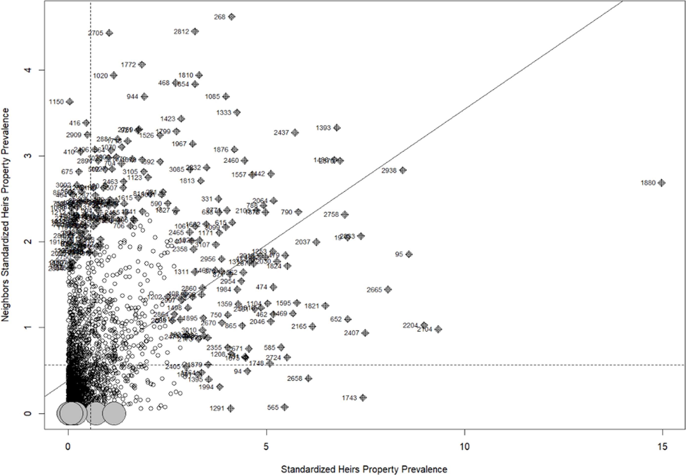
To evaluate the presence of spatial autocorrelation in heirs’ property prevalence across U.S. counties, we employ the global Moran’s I index and LISA map as diagnostic tools, following Anselin (Reference Anselin1995). These tools provide robust methods for assessing whether and how similar values of heirs’ property prevalence cluster spatially across the study area. Global Moran’s I offers a summary measure of the overall spatial autocorrelation in the data set. A statistically significant Moran’s I indicates whether a high or low prevalence of heirs’ property tends to occur in geographically proximate counties. For this study, the global Moran’s I, calculated at 0.315,Footnote 3 is statistically significant at the 1% level, confirming the presence of positive spatial autocorrelation. This result suggests that counties with a high prevalence of heirs’ property are frequently surrounded by other counties with similarly high prevalence, while counties with low prevalence also tend to cluster together.
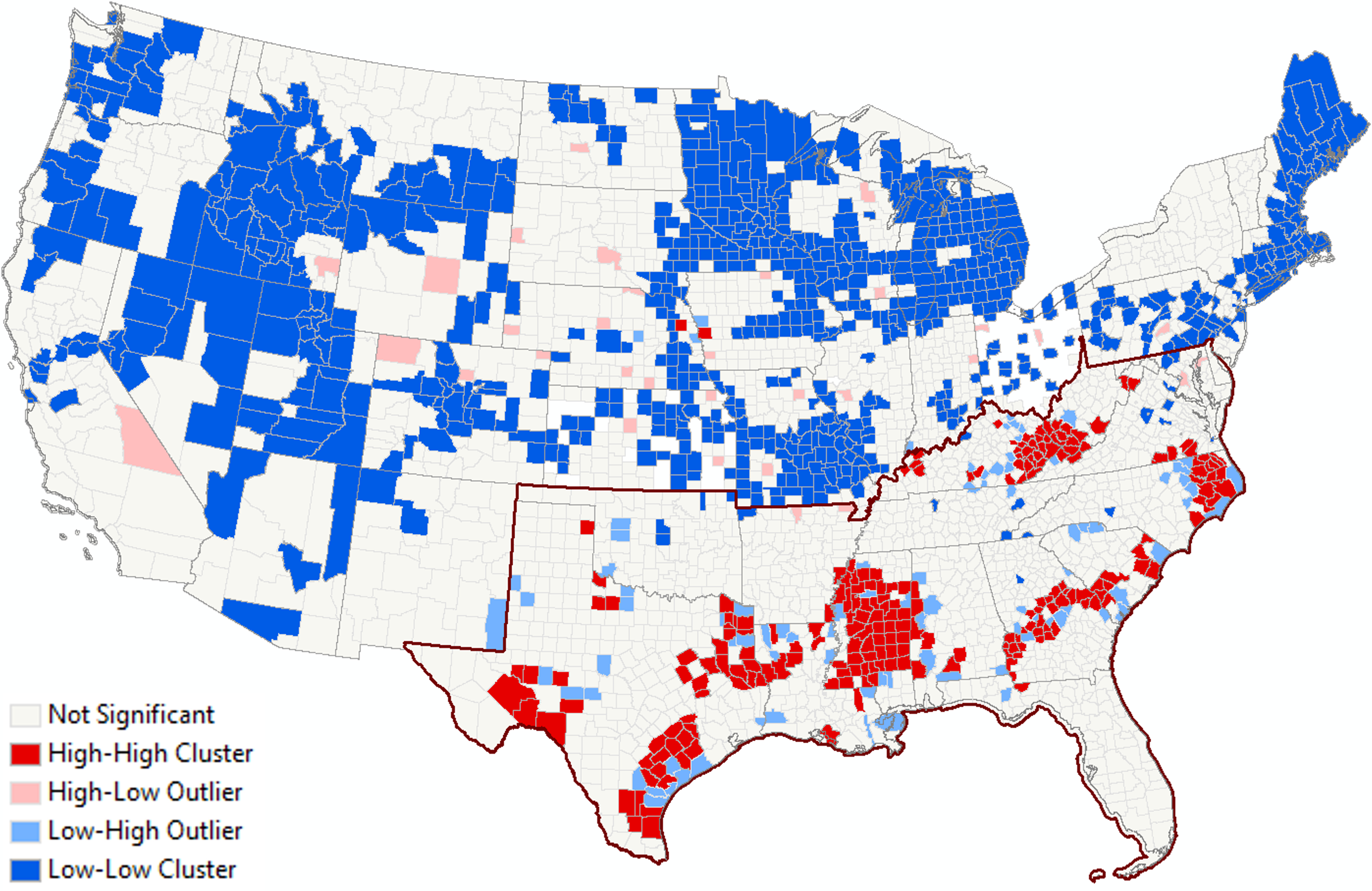
While the global Moran’s I is useful for detecting overall spatial clustering, it does not reveal the specific locations or regional patterns of clusters. To address this limitation, we employ LISA to analyze local spatial autocorrelation. LISA provides a detailed visualization, as shown in Figure 2, identifying specific hot spots and cold spots. Hot spots (high-high clusters in red) represent counties where both a county and its neighbors exhibit high levels of heirs’ property prevalence, while cold spots (low-low clusters in blue) indicate regions where a county and its neighbors exhibit consistently low prevalence. This localized perspective is essential for identifying regional patterns that the global measure cannot capture. These hot and cold spots reflect the positive global autocorrelation result as calculated in the global Moran’s I analysis. Moran’s I and LISA confirm that heirs’ property prevalence is not randomly distributed across space but instead shows clear spatial clustering. These findings suggest that further analysis should account for spatial dependence in both the outcome and residual structure.
Local indicators of spatial association (LISA) map. Note: Local Moran’s I with Queen Matrix and Row Standardized; the red boundary presents the U.S. Census’s South Region.
To address this, we apply a spatial econometric model that accounts for spatial dependence in both the dependent variable and the error term. This allows us to identify not only direct associations between local characteristics and heirs’ property, but also spillover effects across neighboring counties that standard OLS models cannot provide. While concerns have been raised in the literature regarding the use of spatial econometric models, particularly the challenges of causal identification and the construction of spatial weight matrices (Partridge et al. Reference Partridge, Boarnet, Brakman and Ottaviano2012), these models remain valuable tools for characterizing spatial patterns in regional data. In this study, our focus is on describing spatial associations in heirs’ property prevalence and understanding how these associations extend across neighboring counties rather than identifying causal mechanisms.
To account for spatial processes, we utilize spatial models that incorporate spatial lags in the dependent variable $\left( {Wy} \right)$
and/or the error terms
$\left( {Wy} \right)$
and/or the error terms $\left( {Wu} \right)$
, as shown in Equation (1):
$\left( {Wu} \right)$
, as shown in Equation (1):
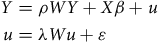 $$\eqalign{ Y & = \rho WY + X\beta + u \cr u & = {\rm{\lambda }}Wu + \varepsilon \cr} $$
where $Y$
is a vector representing the prevalence of heirs’ property, defined as the percentage of heirs’ property parcels out of the total number of parcels in each county;
$Y$
is a vector representing the prevalence of heirs’ property, defined as the percentage of heirs’ property parcels out of the total number of parcels in each county; $WY$
represents the prevalence of heirs’ property in neighboring counties, as defined by the weights matrix;
$WY$
represents the prevalence of heirs’ property in neighboring counties, as defined by the weights matrix; $W$
is a first-order queen-contiguity weights matrix that measures geographic relationships based on all counties sharing boundary pointsFootnote 4;
$W$
is a first-order queen-contiguity weights matrix that measures geographic relationships based on all counties sharing boundary pointsFootnote 4; $X$
is a matrix of independent variables, including socioeconomic, demographic, and geographic factors, such as Black or Hispanic county (dummy variables equal to 1 if more than 30% of the total population belongs to these groups), urban-rural location, poverty rates, income inequality, etc.;
$X$
is a matrix of independent variables, including socioeconomic, demographic, and geographic factors, such as Black or Hispanic county (dummy variables equal to 1 if more than 30% of the total population belongs to these groups), urban-rural location, poverty rates, income inequality, etc.; $\rho $
presents the spatial lag parameter, reflecting endogenous interaction effects among counties; and
$\rho $
presents the spatial lag parameter, reflecting endogenous interaction effects among counties; and ${\rm{\lambda }}$
represents the spatial error parameter, capturing spatial correlation effect in the error terms. The model described in Equation (1) is referred to as the spatial autoregressive combined (SAC) model, as suggested by Kelejian and Prucha (Reference Kelejian and Prucha2010) when
${\rm{\lambda }}$
represents the spatial error parameter, capturing spatial correlation effect in the error terms. The model described in Equation (1) is referred to as the spatial autoregressive combined (SAC) model, as suggested by Kelejian and Prucha (Reference Kelejian and Prucha2010) when $\rho \ne 0$
and
$\rho \ne 0$
and ${\rm{\lambda }} \ne 0$
. This model simultaneously accounts for two distinct spatial processes: spatial lag (
${\rm{\lambda }} \ne 0$
. This model simultaneously accounts for two distinct spatial processes: spatial lag ( $\rho \ne 0$
) and spatial error effects (
$\rho \ne 0$
) and spatial error effects ( ${\rm{\lambda }} \ne 0)$
. The SAC model provides a comprehensive framework for analyzing the interaction of county characteristics and their influence on heirs’ property prevalence.
${\rm{\lambda }} \ne 0)$
. The SAC model provides a comprehensive framework for analyzing the interaction of county characteristics and their influence on heirs’ property prevalence.
To evaluate model performance and the impacts of spatial dependencies, we compare the SAC model with three alternative approaches: an ordinary least squares (OLS) model assuming no spatial dependencies ( $\rho = 0$
and
$\rho = 0$
and ${\rm{\lambda }} = 0$
in Equation (1)), spatial lag (SL) including spatial lags in the dependent variable (
${\rm{\lambda }} = 0$
in Equation (1)), spatial lag (SL) including spatial lags in the dependent variable ( $\rho \ne 0$
and
$\rho \ne 0$
and ${\rm{\lambda }} = 0$
), and spatial error (SE) focusing on spatial correlation in the error terms (
${\rm{\lambda }} = 0$
), and spatial error (SE) focusing on spatial correlation in the error terms ( $\rho = 0$
and
$\rho = 0$
and ${\rm{\lambda }} \ne 0$
). Each model provides unique insights. For instance, the spatial lag model examines how the prevalence of heirs’ property in one county influences its neighboring counties, while the spatial error model identifies spatial dependencies in unexplained variability. The SAC model integrates both spatial lag and error effects, offering a more holistic analysis of spatial relationships.
${\rm{\lambda }} \ne 0$
). Each model provides unique insights. For instance, the spatial lag model examines how the prevalence of heirs’ property in one county influences its neighboring counties, while the spatial error model identifies spatial dependencies in unexplained variability. The SAC model integrates both spatial lag and error effects, offering a more holistic analysis of spatial relationships.
The SAC model is well-suited for contexts in which spatial dependence may arise from both the outcome variable and unobserved factors captured in the error term. By simultaneously incorporating spatial lags and spatial error components, this model offers greater flexibility than single-process models such as the SL or SE model. A strength of the SAC model is its ability to distinguish between endogenous spatial interactions (through $\rho $
), for instance, policy diffusion or land management spillovers, and spatial correlation that may stem from omitted or unobserved regional factors (through
$\rho $
), for instance, policy diffusion or land management spillovers, and spatial correlation that may stem from omitted or unobserved regional factors (through ${\rm{\lambda }}$
). However, SAC models also rely on strong assumptions regarding the structure of spatial relationships, and interpretation of the results requires caution, especially when causal mechanisms are not explicitly identified (McMillen Reference McMillen2012; Partridge et al. Reference Partridge, Boarnet, Brakman and Ottaviano2012). Despite these limitations, the SAC model is appropriate for our study given its ability to capture both direct and spillover effects in a setting where regional clustering is empirically evident but not structurally simple.
${\rm{\lambda }}$
). However, SAC models also rely on strong assumptions regarding the structure of spatial relationships, and interpretation of the results requires caution, especially when causal mechanisms are not explicitly identified (McMillen Reference McMillen2012; Partridge et al. Reference Partridge, Boarnet, Brakman and Ottaviano2012). Despite these limitations, the SAC model is appropriate for our study given its ability to capture both direct and spillover effects in a setting where regional clustering is empirically evident but not structurally simple.
The reduced form of Equation (1) is given by:
 $$Y = {\left( {I - \rho W} \right)^{ - 1}}X\beta + {\left( {I - \rho W} \right)^{ - 1}}{\left( {I - {\rm{\lambda }}W} \right)^{ - 1}}\varepsilon$$
From this reduced form, we derive direct and indirect effects, which reflect the spatial structure, i.e. ${\left( {I - \rho W} \right)^{ - 1}}\beta $
. The direct effects of socioeconomic variables (
${\left( {I - \rho W} \right)^{ - 1}}\beta $
. The direct effects of socioeconomic variables ( $X$
on heirs’ property) are defined by the mean of the diagonal terms of the matrix
$X$
on heirs’ property) are defined by the mean of the diagonal terms of the matrix ${\left( {I - \rho W} \right)^{ - 1}}\beta $
. The indirect effects (spillover effects) capture the influence of neighboring countries’ characteristics on the focal county’s prevalence by being represented as the mean of the off-diagonal terms. These effects are important for understanding both localized and regional drivers of heirs’ property, as summarized in Table 4.
${\left( {I - \rho W} \right)^{ - 1}}\beta $
. The indirect effects (spillover effects) capture the influence of neighboring countries’ characteristics on the focal county’s prevalence by being represented as the mean of the off-diagonal terms. These effects are important for understanding both localized and regional drivers of heirs’ property, as summarized in Table 4.
Data
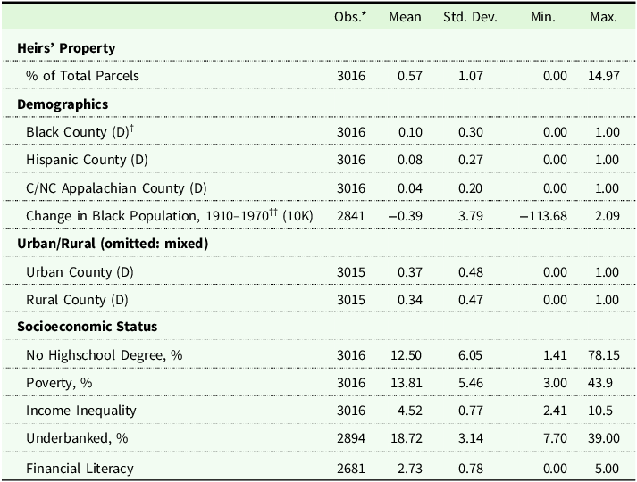
The measurement of variables and the data sources are presented in Table 1.
Definitions of variables and sources of data
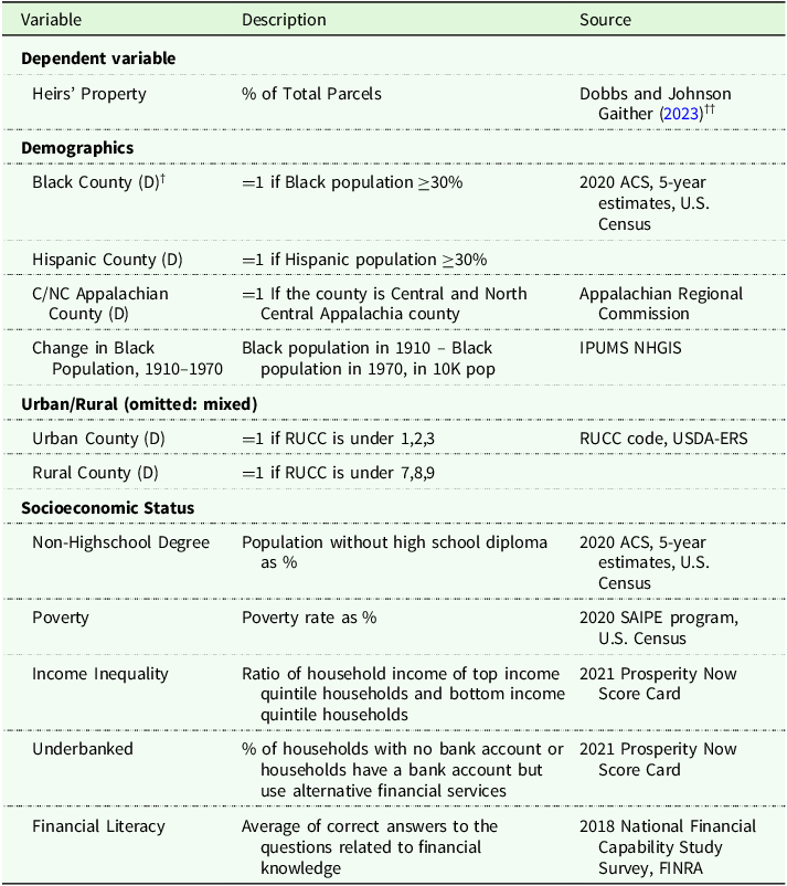
Note: †(D) presents dummy variable, otherwise Continuous; USDA (U.S. Department of Agriculture); ACS (American Community Survey); IPUMS NHGIS (National Historical GIS); RUCC (Rural-Urban Continuum Codes); USDA-ERS (Economic Research Service); SAIPE (Small Area Income and Poverty Estimates) program; FINRA (Financial Industry Regulatory Authority). ††We utilize heirs’ property prevalence rates provided by Dobbs and Johnson Gaither, which were derived from the March 2021 LightBox data set. Their published study (Dobbs and Johnson Gaither, Reference Dobbs and Johnson Gaither2023) uses a later version of the LightBox data set from November 2021, and readers should be aware of potential differences in estimates.
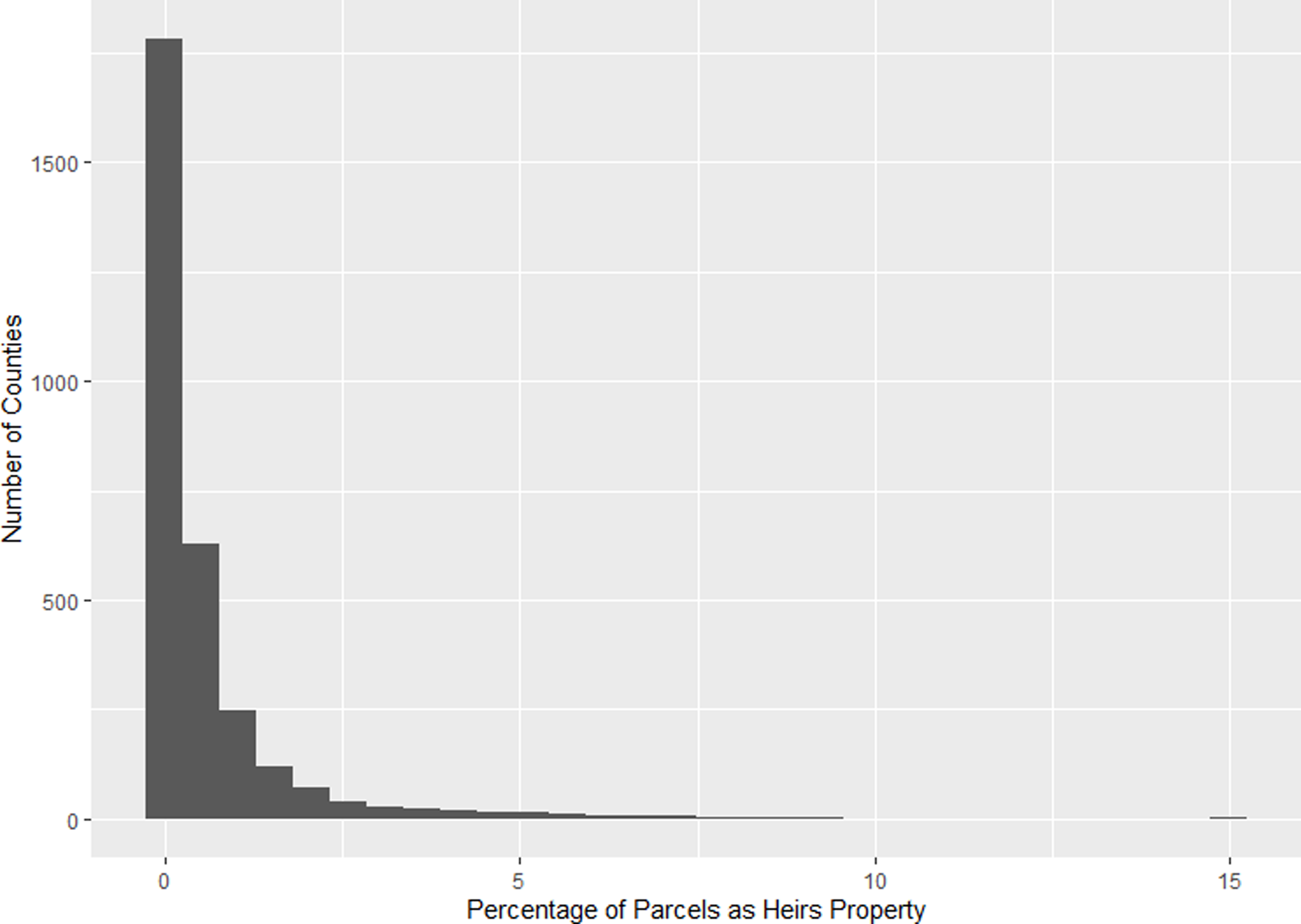
Our analysis uses county-level data from 2021, with the dependent variable defined as the prevalence of heirs’ property as a percentage of total parcels. The data on heirs’ property and total parcels were derived from Dobbs and Johnson Gaither’s (Reference Dobbs and Johnson Gaither2023) study, which provides detailed descriptions of the geoprocessing and estimation methodologies used to quantify the number of heirs’ property parcels. On average, heirs’ property parcels account for 0.57% of all parcels in a county. However, the distribution is highly right-skewed: while most counties report less than 1%, a small number exhibit prevalence rates approaching 15% (see Figure A.2 in the Appendix).
Building on prior research, we include a comprehensive set of demographic, socioeconomic, and geographic variables that are presumably positively or negatively associated with the prevalence of heirs’ property. Most variables are drawn from previous research related to heirs’ property. Additionally, we account for historical events such as the “Great Migration” of African Americans from the U.S. South to northern, midwestern, and western U.S. cities from about 1910 to 1970. This exodus is associated with declines in African American-owned land in the South (Mitchell Reference Mitchell2001). This historical event is represented by the change in the Black population over that period, reflecting its impact on land ownership patterns. We also include variables of income inequality, the percentage of underbanked households, and financial literacy level in the county to test their association with the occurrence of heirs’ property. As mentioned in the literature review section, heirs’ property is common in rural southern counties with larger Black populations, southwest counties with high Hispanic populations, and Appalachian counties with high White populations. These counties are generally characterized by higher poverty rates and lower levels of educational attainment (Bobroff Reference Bobroff2001; Deaton Reference Deaton2007; Johnson Gaither Reference Johnson Gaither2016; Johnson Gaither and Zarnoch Reference Johnson Gaither and Zarnoch2017). Summary statistics are shown in Table 2.
Descriptive statistics

Note: †(D): Dummy Variable; ††Change in Black Population, 1910–1970 is calculated as the population in 1970 subtracts from the population in 1910. *While there are 3,144 counties in the contiguous U.S., heirs’ property data are not available for all counties. The primary data set includes 3,016 counties with valid heirs’ property estimates, and most of the variables are matched to this subset. Other variables, such as urban/rural counties, historical changes in Black population, underbanked households, and financial literacy, also have missing values at the county level, resulting in slightly fewer observations for some measures.
Estimation results
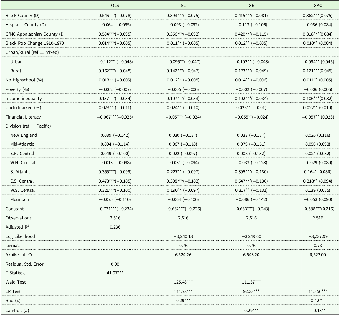
Table 3 presents the estimation results from the ordinary least squares (OLS) model and three spatial econometric models: spatial lag (SL), spatial error (SE), and SAC. While these models share similar identification strategies to capture spatial relationships, they employ distinct estimation techniques, which preclude direct comparison of their coefficients. Specifically, the estimates from SL, SE, and SAC should not be interpreted as marginal effects in the same manner as those from the OLS model. Instead, our discussion focuses on the directions of estimates, statistical significance, and relevant statistical information.
Estimation results of OLS and spatial models

Notes: ***, **, and * indicate 1%, 5%, and 10% levels of significance, respectively; standard errors in parentheses; SL for spatial lag, SE for spatial error, and SAC for spatial autoregressive combined model.
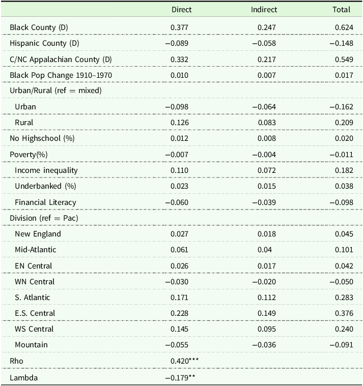
Direct/indirect impact of SAC

All models indicate that heirs’ property is predominantly a Southern phenomenon. Positive, statistically significant estimates are observed exclusively for Census divisions in the South region (South Atlantic, East South Central, and West South Central divisions), with the exception of the West South Central division in SAC model. These findings are consistent with the OLS results when using various regional variables (see Table A.1 in the Appendix). In the models that include a South region dummy variable, only variables related to the South exhibit statistically significant positive estimates across the four regions (referred to West), and nine divisions (referred to Pacific). These results align with prior studies emphasizing the regional clustering of heirs’ property in the South.
The empirical findings partially corroborate earlier research. Counties with a high percentage of Black residents (more than 30% of the population, represented by the Black County dummy variable) consistently exhibit a positive and statistically significant relationship with heirs’ property prevalence across all models. Similarly, counties in Central and North Central Appalachia, which have high percentages of White residents, also show statistically significant and positive correlations with heirs’ property. However, Hispanic-majority counties (more than 30% of the population, represented by the Hispanic County dummy variable) do not demonstrate statistically significant results. The findings also reveal that heirs’ property prevalence is higher in rural areas compared to urban or mixed urban-rural areas, underscoring the rural nature of this issue.
Among economic variables, income inequality appears to be more closely associated with heirs’ property than the poverty rate, which is often presumed to be primarily related to heirs’ property. However, our study does not find a statistically significant correlation between the prevalence of heirs’ property and poverty in any model, suggesting that disparities in income distribution, rather than absolute poverty, may better explain heirs’ property prevalence. Variables related to financial environments, such as financial access (underbanked) or the level of financial knowledge (Financial Literacy), further show some association with heirs’ property. Counties with higher proportions of underbanked households show a significant positive association with heirs’ property prevalence, while counties with greater financial literacy exhibit a negative relationship. These results suggest that both access to financial services and financial knowledge can play roles in mitigating heirs’ property issues.
OLS estimates tend to overstate the magnitude of coefficients without accounting for endogeneity from spatial dependence. The SAC model, which incorporates spatial interactions and correlation in the dependent variable ( $\rho $
) and error terms (
$\rho $
) and error terms ( ${\rm{\lambda }}$
), provides a more robust framework for analyzing heirs’ property prevalence while demonstrating better statistical characteristics. In our results, the spatial lag coefficient from the SAC model is positive (ρ = 0.42) and statistically significant, indicating that counties with high heirs’ property prevalence are more likely to be located near other counties with similarly high prevalence. This pattern is consistent with the spatial clustering confirmed by Moran’s I and LISA. The SAC model also yields a statistically significant negative spatial error parameter (λ = –0.18), suggesting that once spatial interaction is captured in the dependent variable, the remaining unexplained variation is more spatially dispersed. This contrasts with the SE model, where λ is positive (0.29), implying that some of the spatial correlation in the residuals was previously misattributed to unobserved factors.
${\rm{\lambda }}$
), provides a more robust framework for analyzing heirs’ property prevalence while demonstrating better statistical characteristics. In our results, the spatial lag coefficient from the SAC model is positive (ρ = 0.42) and statistically significant, indicating that counties with high heirs’ property prevalence are more likely to be located near other counties with similarly high prevalence. This pattern is consistent with the spatial clustering confirmed by Moran’s I and LISA. The SAC model also yields a statistically significant negative spatial error parameter (λ = –0.18), suggesting that once spatial interaction is captured in the dependent variable, the remaining unexplained variation is more spatially dispersed. This contrasts with the SE model, where λ is positive (0.29), implying that some of the spatial correlation in the residuals was previously misattributed to unobserved factors.
The shift from a positive λ in the SE model to a negative λ in the SAC model, accompanied by an increase in ρ from 0.29 (SL) to 0.42 (SAC), suggests that the SAC model reallocates spatial dependence more accurately between the structural and residual components. The SL model captures spatial dependence only in the dependent variable and may therefore underestimate the extent of direct spatial interaction. By accounting for both lag and error processes simultaneously, the SAC specification offers a clearer picture of spatial dependence in heirs’ property. This dual structure helps disentangle the effects of observed spatial interaction from those arising due to unobserved or omitted regional factors. This capacity to separate multiple sources of spatial correlation reinforces the appropriateness of the SAC model for understanding the spatial dynamics of heirs’ property prevalence. Therefore, the SAC model forms the basis for deriving direct, indirect, and total effects, which provide insights into the spatial dynamics of heirs’ property.
In contrast to OLS, which yields a single point estimate for each covariate’s impact on the outcome variable, spatial econometric models produce a full matrix of effects that reflect both direct and indirect (spillover) influences across spatial units. This richer structure accounts for the fact that a change in a covariate in one county can influence not only that county’s outcome but also outcomes in neighboring counties, and potentially feed back into the origin county through higher-order spatial interactions. Following LeSage and Pace (Reference LeSage, Pace, Fischer and Getis2010), we summarize these complex relationships using average direct, indirect, and total effects, which provide an interpretable representation of spatial dynamics in our data. This matrix-based framework allows for a more nuanced understanding of how local characteristics and spatial spillovers jointly shape the observed geographic patterns in heirs’ property prevalence.
Table 4 presents the direct, indirect, and total effects derived from the SAC model, following the approach of LeSage and Pace (Reference LeSage, Pace, Fischer and Getis2010). As noted above, the estimates of the SAC model in Table 3 do not directly represent the marginal effects of the independent variables on the dependent variables. Direct effects reflect the impact of changes in the independent variables on heirs’ property prevalence in a focal county, while indirect effects capture spillover impacts that pass through neighboring counties and feed back into the focal county.
Total effects represent the combined direct and indirect effects. For instance, the direct effect of the Black County dummy variable is estimated at 0.377, indicating that the prevalence of heirs’ property increases by 0.377 percentage points in counties where Black residents constitute over 30% of the population. The indirect effect is 0.247, suggesting that the presence of neighboring Black-majority counties contributes an additional 0.247 percentage points to heirs’ property prevalence in the focal county through spatial spillovers. These feedback effects are partially due to the coefficient of the spatially lagged dependent and the spatial correlation in the error terms. Combining both effects, the total effect of the Black County variable on the heirs’ property prevalence is 0.624 percentage points.
The results from Table 4 provide additional insights into the drivers and patterns of heirs’ property prevalence. First, regional clustering is evident, with the East South Central and South Atlantic divisions exhibiting strong total effects with statistical significance. It highlights the regional nature of the heirs’ property issue. Second, major factors associated with heirs’ property prevalence include being a Black county, being located in Central and North Central Appalachian counties, and experiencing high levels of income inequality in rural areas. Economic and financial-related factors, such as income inequality, underbanked households, and financial literacy, show significant effects, underscoring the importance of financial and economic environments. Income inequality is particularly influential, with both direct and indirect effects demonstrating its strong association with heirs’ property prevalence. Rural counties exhibit higher total effects than urban or mixed urban-rural counties, reinforcing the rural concentration of heirs’ property challenges.
The Great Migration, as measured by changes in the Black population between 1910 and 1970, is limited in association with heirs’ property prevalence in 2021, though it accounts for some variation. These findings underscore the importance of addressing heirs’ property through a combination of socioeconomic and spatially targeted interventions. Spatial spillover effects, as captured by indirect effects, suggest that resolving heirs’ property issues in one county could positively influence neighboring areas.
In summary, rural counties–particularly those classified as Black counties, located in Central and North Central Appalachia, and with high levels of income inequality–are more likely to have a higher prevalence of heirs’ property. Financial environments, such as limited banking access and low financial literacy, also contribute to this phenomenon. While the magnitude of indirect effects, which capture the influence of neighboring counties on the prevalence of heirs’ property in the focal county, is smaller due to the nature of spatial spillovers, the patterns of influence remain consistent with the direct impact. These findings suggest that counties surrounded by rural counties with similar characteristics are also more likely to experience higher levels of heirs’ property prevalence. The results highlight the need for regional and multi-county strategies to address heirs’ property challenges and promote broader equity and development.
Conclusion and discussion
Heirs’ property is a longstanding issue that is complicated and tangled with history, politics, and social inequities. Efforts by federal and local governments, community leaders, and researchers have worked through various channels to address the complex challenges posed by heirs’ property. Understanding this phenomenon from spatial and socioeconomic perspectives requires not only identifying where heirs’ properties are located and whether they exhibit spatial clustering but also how regional and socioeconomic factors correlate with their prevalence. Previous research has often addressed these questions in relatively small areas, limited to multiple counties or communities, primarily due to data availability and data collection challenges. Advancements in geoprocessing technology and big data handling have facilitated the estimation of heirs’ property across the U.S. and enabled the utilization of heirs’ property data spanning all U.S. counties, thereby contributing to the evolving literature on this topic.
Our analysis reveals, first, that heirs’ property exhibits spatial autocorrelation with clustering in the southern U.S. This finding highlights the historical and regional distinctiveness of the issue, particularly in areas with high proportions of Black population, location in Appalachia and rural counties. Second, among the spatial econometric models we examined, the SAC model is appropriate for analyzing heirs’ property prevalence, accounting for spatial dependence. This model provides empirical evidence to support the correlation of heirs’ property prevalence with characteristics identified in earlier studies.
The analysis also uncovers socioeconomic relationships that previous research has not fully explored. Notably, income inequality is more strongly associated with heirs’ property prevalence than poverty, highlighting an oversight in previous studies that emphasized poverty as the primary associated factor without considering income inequality. While our analysis does not aim to establish causality, it is possible that the relationship between heirs’ property and income inequality is bidirectional. A limited ability to formalize property ownership may constrain wealth-building opportunities, such as using land as collateral, accessing government programs, or passing assets intergenerationally, which could reinforce local patterns of inequality.
Financial environments also play a role. Counties with high rates of underbanked households and lower levels of financial literacy show significantly higher correlations with greater heirs’ property prevalence. These results underscore the broader financial and economic challenges linked to heirs’ property beyond traditional socioeconomic indicators like educational attainment and poverty rates. The results are consistent with the idea that socioeconomic and financial disadvantages, such as limited income, low financial literacy, or restricted access to financial services, may reduce the likelihood of formal estate planning and thereby increase the likelihood that property remains in heirs’ property form without clear title. This pathway helps explain how structural inequalities can translate into legal and economic vulnerabilities across generations.
In addition, the study reveals the importance of spatial spillover effects observed through direct and indirect channels. The spatial spillover results suggest that heirs’ property prevalence in one county may be associated with that in nearby counties through shared economic conditions, legal environments, or cultural norms. Counties within the same region may face similar estate planning barriers, a lack of legal resources, or land tenure customs. These overlapping conditions may explain why the prevalence of heirs’ property tends to cluster across adjacent counties. Efforts to resolve heirs’ property issues in one county–through title clearing initiatives, financial support programs, or community education–may positively influence neighboring counties by reducing prevalence and improving economic conditions. This finding emphasizes the interconnected nature of the issue, reinforcing the need for regional or multi-county strategies rather than isolated and county-specific interventions. Such approaches are critical for addressing heirs’ property’s compounded vulnerabilities and fostering equitable regional development.
Our findings contribute to the growing body of research on heirs’ property, providing valuable insights for local leaders or practitioners with limited resources. These insights can help identify communities and target groups most in need of assistance, particularly in regions with a high prevalence of heirs’ property. Despite these contributions, our study has certain limitations. By relying on cross-sectional data, the analysis may not fully capture the temporal dynamics of heirs’ property over time and across space. The focus on associations between county factors and heirs’ property prevalence does not delve into the underlying causes or consequences of this phenomenon. Future research could address these limitations by employing longitudinal data or quasi-experimental designs to explore causal relationships and temporal trends.
Another direction for future research involves examining the impact of the Uniform Partition of Heirs Property Act (UPHPA), which, as of 2025, has been enacted in over 20 U.S. states. While this study does not incorporate UPHPA, the legislation represents a policy intervention aimed at protecting heirs’ property owners from involuntary loss through partition sales. Assessing the effect of state-level UPHPA adoption on heirs’ property prevalence could offer new insights into the role of legal frameworks. This approach would require a causal framework, leveraging quasi-experimental methods, to examine whether the legislation has had measurable effects on reducing heirs’ property, particularly after controlling for other socioeconomic confounders. Furthermore, incorporating alternative data sources of heirs’ property, such as estimates by Thomson and Bailey (Reference Thomson and Bailey2023), could validate and expand upon our findings, potentially uncovering spatial and socioeconomic patterns.
In conclusion, our findings contribute to the evolving understanding of heirs’ property by comprehensively analyzing its spatial distribution and socioeconomic determinants. Policy makers and practitioners can use these insights to identify high-prevalence regions and target interventions for the most affected communities. Addressing heirs’ property requires collaborative, regionally coordinated strategies that promote equity and sustainability, ensuring that the historical burdens of this issue do not continue to hinder future generations.
Data availability statement
Most of the data used in this study are publicly available. The heirs’ property data set, which was provided by co-authors Dobbs and Johnson Gaither, is not available but may be shared upon reasonable request.
Acknowledgements
We gratefully acknowledge the helpful comments of two anonymous reviewers and Editor Anna Klis.
Funding statement
The project was supported by the Agricultural and Food Research Initiative Competitive Program of the USDA National Institute of Food and Agriculture (NIFA) under Grant Number 2021-67023-34425. Any opinions, findings, conclusions, or recommendations expressed in this publication are those of the authors and should not be construed to represent any official USDA or U.S. Government determination or policy. Development of the Heirs’ Property data set used in this study was supported by the Oak Ridge Institute for Science and Education (ORISE).
Competing interests
The authors declare that they have no potential conflicts of interest.
Appendix
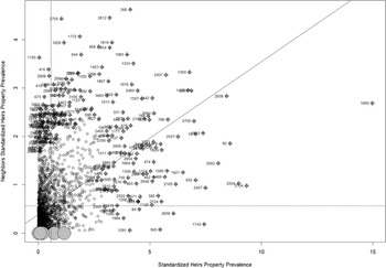
Moran Scatter Plot of Heirs’ Property Prevalence (Moran’s I = 0.315, at 0.1% level).
Distribution of Heirs’ Property Prevalence across Counties.

OLS Results: Comparison of Regional Effects
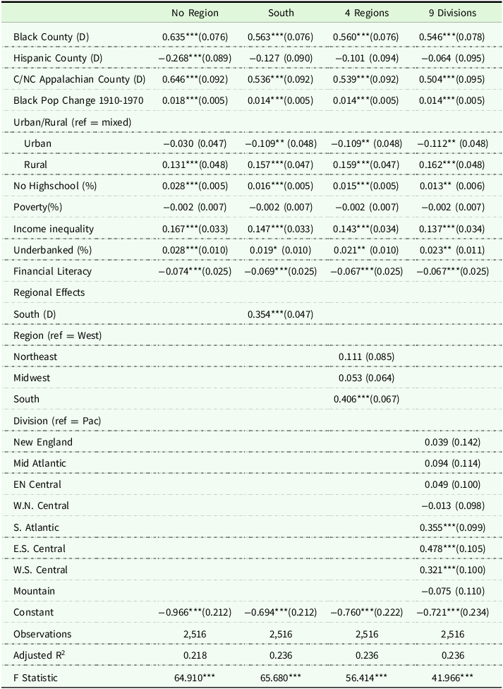
Notes: ***, **, and * imply 1%, 5%, and 10% levels of significance, respectively; standard errors in parentheses.


 Open access