

1. Introduction
The car insurance market is globally the most important line of business in the property and casualty insurance market due to high premium volume. In Europe, the motor vehicle business represents with €130 billion in 2013 a share of about 29% of the total premium volume (see Insurance Europe, 2014). In view of significant technological changes such as assistance systems, connected or driverless cars, it is very difficult to forecast the future of car insurance. The so-called telematic box is an intermediate step in terms of technology, which can change the rules of the pricing structure. Telematic data enable innovative, usage-based insurance premium models known as pay-how-you-drive (PHYD) insurance, but in this regard they represent a special challenge for actuaries because of their complexity and volume.
Existing studies provide different insights into telematic insurance solutions. However, empirical studies on the implementation into actuarial pricing methods are still very limited. Jun et al. (Reference Jun, Ogle and Guensler2007, Reference Jun, Ogle and Guensler2011) work out the relationship between mileage as well as velocity parameters and accident risk, whereas Kremslehner & Muermann (Reference Kremslehner and Muermann2013) examine the effect of the number of car rides, the relative distance driven on weekend, respectively, at night and the average speeding on risk. Toledo et al. (Reference Toledo, Musicant and Lotan2008) determine risk indices and statistics identifying manoeuvre types with methods, which are not specified in detail. A classification analysis approach for aggregated pay-as-you-drive (PAYD) rate factors to actuarial decision making with vehicle sensor data are provided in Paefgen et al. (Reference Mangiameli, Chen and West2013). Currently, either in science or in practice there is no standardised method to achieve a clear “score” of driving behaviour; telematic approaches from abroad do not extend to the very precise German actuarial pricing due to the limited scope of their scoring methods (see Karapiperis et al., Reference Karapiperis, Obersteadt, Brandenburg, Castagna, Birnbaum, Greenberg and Harbage2015). In general, a priori and a posteriori risk profile building should be included in a comprehensive model. What is missing therefore is an effective approach for the solid evaluation of driving profiles on the basis of the limited data available, and in particular without recourse to the claims situation which is not available.
This paper wants to give a realistic and useful evaluation method for driving profiles, which in turn can be used for innovative, optimised car insurance pricing in the private client segment due to reduction of information asymmetry with regard to the user group. Our analysis uses a vehicle mobility model for generating potential driving profiles, which grants our study a sound, broad data basis. We link the model results to real-world data of a telematic portfolio of a large German car insurer. We determine driving styles of generated driving profiles creating the basis for a general risk categorisation and validate the results by comparing them with empirical data. The combination of model results and the empirical data allows us to directly test whether a differentiation according to predefined driving styles is possible and how well the data format fits to make a valid statement on the driving styles. Furthermore, we can define a first minimum data request.
Our results not only contribute to academic research, but are also of high relevance and usefulness to insurance practice. A fundamental finding is that specific driving styles can be derived from driving profiles based on validated velocity and acceleration parameters even under consideration of severe privacy protection issues. These styles can form the basis for a risk categorisation and thus for subsequent discounts or surcharges on the premiums dependent of the driving behaviour.
The remainder of this paper is divided into four sections. First of all, the key actuarial pricing aspects in German car insurance pricing are introduced, including innovative pricing strategies. In section 3, the development of driving styles based on data using a mobility model and the process of empirical data collecting are presented. Section 4 discusses the results from the empirical study. The paper closes with conclusions and limitations of our work, and outlines suggestions for further research.
2. Overview of German Car Insurance Pricing
2.1. Current pricing strategy
The pricing of German motor vehicle insurance is based on numerous relevant factors – more than any other segment in the German property and casualty insurance. Various subjective and objective tariff criteria, as well as numerous criteria for discounts influence the insurance premium (see e.g. Stadler, Reference Stadler2008; Laas et al., Reference Lange2014). This can be attributed to the increased importance of risk-adjusted premiums after the deregulation of the European Union insurance markets in 1994. A comparison of the average annual premiums and losses for each risk shows that the price is aligned to the risk over time (see Figure 1). The most important prerequisite for adequately projecting the actual risk is the selection of different, suitable and tariff-related risk characteristics.
Average annual premiums and losses in the German motor vehicle third-party liability insurance from 2000 until 2013 (see Gesamtverband der Deutschen Versicherungswirtschaft e.V., Reference Gerpott and Berg2012).

The German insurance industry distinguishes between objective and subjective criteria. Objective criteria concern the vehicle and a priori are independent of the policyholder’s individual risk behaviour. These include, e.g., the type of vehicle, type classification and age of vehicle at the time of purchase. In contrast, subjective criteria relate to the person to be insured. Such criteria include the bonus-malus level, regional classification, occupation and age of the policyholder and users or the annual mileage performance (see e.g. Heep-Altiner & Klemmstein, Reference Heep-Altiner and Klemmstein2001). Discounts such as home ownership, a garage or a workshop affiliation in the event of damage represent other factors (see e.g. Stadler, Reference Stadler2008; Laas et al., Reference Lange2014).
The set of tariff criteria separates policies into groups, so-called tariff classes. From the historical claims data an expected average annual loss is determined for each tariff class, which corresponds to the size of the net premium (see e.g. DAV-Arbeitsgruppe Tarifierungsmethodik, 2015). Therefore, a large quantity of pricing variables induces a large dimensionality of an actuarial table. This fact in turn leads to an increasingly covert and complex market, of the one part, and high calculation capacity for the actuaries, of the other. Indeed, it can be seen that, in recent years, the insurers continuously introduce more and more subjective criteria (see Domeyer, Reference Domeyer2005; Laas et al., Reference Lange2014; Hartmann & Nützenadel, Reference Hartmann and Nützenadel2015). There are several reasons for this: the increasing knowledge of the actuarial risks due to the rising personal data availability in the course of electronic data processing, the high competitive pressure and not least the unisex judgement. This is done to calculate the tariffs more risk adjusted and more individualised.
2.2. Innovative pricing strategies
Each year, the German Insurance Association (GDV) submits a tariff recommendation for their member companies. Thus, a harmonised method of calculating tariffs has been established in Germany. Nowadays, the premium amount depends highly on the classification into a bonus-malus system. In the third-party liability and fully comprehensive insurance, a no-claims discount is set individually for each policy and is determined by the respective insurer on the basis of the bonus-malus level; the no-claims discount does not exist in the partially comprehensive insurance. Furthermore, any insurance company records statistical data, such as the insurance regional and type classification, and takes soft factors, such as age of users, group of users and occupation of the policyholder into account when setting premiums. However, the tariffs differ between the various insurance companies – the insurance companies deviate more or less from the recommendation of the GDV in some criteria, e.g., in order to meet the legal requirements of the principle of equal treatment or to regulate migration movements and selection effects (see DAV-Arbeitsgruppe Tarifierung, 2007; Laas et al., Reference Lange2014). This includes the age group of the policyholders due to the lack of social acceptance because the age is not an acceptable reason for discrimination. Therefore, the first and simplest idea to determine the premiums more risk adequately is to use the tariff criteria of the GDV correctly.
Apart from this, pricing according to driving behaviour, as shown in Figure 2, is another possibility to explore in order to achieve the aim of more individualised premiums (see Weidner & Weidner, Reference Weidner and Weidner2014). Here, the emphasis has been placed on GPS technology (telematic) with such aspects as velocity, acceleration, road type, time of day and weather condition. Various sensors like GPS are required for measuring these parameters. Indeed, modern car technology is quite advanced and some sensors are even part of the standard equipment of each vehicle. On the basis of so-called variables of driving behaviour and driving situation (see Gerpott & Berg, 2012), the driving style and performance can be evaluated. Finally, the insurance premium can be aligned with the risk tolerance of the driver. Customers who drive safely and defensively should pay lower premiums in a telematic tariff, whereas customers who drive risky and aggressively should pay higher premiums. Such PHYD systems are already well established in the United States and in Great Britain; in the United States, every seventh new contract is based on telematics (see Stiftung Warentest, 2014). Meanwhile in Germany, first insurers now offer telematics products, which grant discounts on the premiums calculated with traditional tariff criteria.
Conventional and telematic pricing idea comparison.

The evaluation of the two pricing approaches (see Figure 2 to the right) shows that the inclusion of telematic data in the premium calculation is associated with great benefits in particular for differentiated tariffs. This is the result of two factors: first of all, the concrete verification of driving profiles of specific driver-vehicle units at the telematic portfolio level, second, the weighting of differing driving behaviour at the level of a single driver as well as within a user group (see Figure 3). With conventional tariff criteria, only vehicle and user group can be evaluated – not the actual driving behaviour. This has concrete implications to conventionally derived risk groups, where average premiums are calculated based upon the average claims requirement from the respective risk categories (see Figure 4 to the left). For example, novice drivers as a collective user group feature, on average, have a much higher claims requirement than more advanced drivers. Using only the conventional tariff criteria “novice driver”, the calculated claims category for every driver from this user group is identical, thus implying same risk exposure and same premium. Telematic variables on the other hand allow for a differentiated perspective on individual driving styles, such that deviations from the average risk exposure (see Figure 4 to the right) can be identified and incorporated into the risk category classification. Ultimately, this will enable insurers to partly remedy information asymmetry as far as risks depending on actual driving behaviour are concerned. Excess value is created for recently closed contracts, where the bonus-malus level as major tariff criterion is not yet adapted to the actual risk due to missing perennial claims experience. On the other hand, there also exists information asymmetry concerning different users of a vehicle. Although the policyholder is required to name additional vehicle drivers, their usage can only be understood in terms of averages entering into the analysis of claims requirement. For an individualised risk assessment of a contract of a 45-year-old father including his 18-year-old son, the precise attribution of both usage time and risk associated with driving behaviour is critical for understanding the correct claims requirement – especially if both vehicle users exhibit vastly different usage patterns. These usage patterns are one of the key elements telematic analysis of driving behaviour can reveal.
Schematic definitions of abstraction levels.

Valuation perspective of pricing according to conventional and telematic criteria using the example of a user group consisting of single drivers.

A particular challenge regarding the successful implementation of a telematic product regards data protection issues. Complex motion profiles can be generated collecting telematic variables concerning the driving behaviour and the use of vehicle. Therefore, strict data protection criteria are applied to all processes used for the telematic tariff so that the insurer is able to adhere to all of the respective national privacy rules at all time. Concerning the German insurer’s perspective, the prime principles of data minimisation and data avoidance in accordance with section 3, German Data Protection Act (BDSG) as well as the national data protection norms of the German insurance industry themselves, the Code of Conduct, processing or using as little personal data as possible, must be considered. Moreover, it must be ensured that every collected data point actually affects the tariff system complying with the purposeful limitation principle according to the BDSG under which personal data should only be collected and processed for specified and explicit purpose.
As regards the formal feasibility, the technical conditions are already in place, although it is essential to determine the measuring and transmission logic. The application of telematic technology is in particular among forerunners in the external data to optimise the pricing. Applicability of other approaches is possible but not as far developed as telematics (see Weidner & Weidner, Reference Weidner and Weidner2014) – they will certainly be discussed, once their respective technologies reach a level of mass market sophistication, like telematics do now.
Note that there are various outstanding issues as far as the applicability for pricing of the telematic approach is concerned. Beside the question of a suitable choice of telematic tariff criteria, particularly the handling of the missing risk experience is also of major relevance to be able to put the approach into perspective with conventional pricing. This means that the premiums according to the driving behaviour cannot be directly determined based on the analysis of the claims requirements as the pricing is normally made. For this reason, the present approach investigates the pricing innovation that various premium discounts will be granted to the policyholders depending on their style of driving which requires a certain classification of driving behaviour. The discount on the premium per contract will be the weighted evaluation of all the driving styles belonging to the insured vehicle, because our analysis allows differentiating between different driving styles both for individual drivers as well as a mixed group of vehicle users. However, it is obvious that scoring of such differentiated findings requires further research in order to allow for risk adequacy premiums. Finally, the resulting simplified actuarial pricing process is shown in Figure 5.
Incorporation of telematic data in the actuarial pricing process.

3. Telematics Technologies: Evaluation of Driving Behaviour
3.1. Methodology
The procedure for the statistical analysis of driving profiles requires high-quality data and a broad database to achieve sufficient pricing precision. As representativity of the early stages of the empirical telematic portfolio can neither be trusted nor easily verified with the existing lack of claims experience, the most efficient way to build a reliably precise telematic database is extensive stochastic modelling. Therefore, a vehicle mobility model is used for stochastic simulation of driving profiles. The modelling is based on the random waypoint (RWP) principle (see Johnson & Malz, Reference Johnson and Malz1996). Weidner et al. (Reference Weidner, Weidner and Transchel2015) provide a detailed introduction to the method, whereas the modified underlying assumptions are listed in the Appendix. The main point about choosing kinematic observables for this investigation is the realisation that contextual quantities describing the driving situation by likes of road type, maximal acceleration strength or time of day, which are currently in use in telematic assessments (see Karapiperis et al., Reference Karapiperis, Obersteadt, Brandenburg, Castagna, Birnbaum, Greenberg and Harbage2015), can be treated like classical risk factors, whereas for the driving behaviour, given by the actual movement of the vehicle, this is not the case.
The RWP model, slightly modified for this approach, describes the movement behaviour of a driver-vehicle unit in a given system area. Each movement occurs in a manner, such that a driver-vehicle unit randomly selects a destination (waypoint) in the area and a respective speed limit. The driver-vehicle unit moreover moves to this destination with its specific vehicle and driver characteristics, i.e. desired velocity depending on speed limit, specific acceleration rate and brake performance, and pauses for a certain time before selecting a new destination and speed. In this way, a stochastic simulation run generates simultaneously several thousand routes and types of drivers, from which specific driving profiles can be derived (see Figure 6). The choice of model parameters was made such that a wide range of individual characteristics of the driver-vehicle units and specific local conditions are depicted focussing on the representation of average city and rush-hour traffic. The present analysis of driving profiles is based on 10,000 driver-vehicle units, each with a sequence of 20 waypoints. Sampling frequency was set to 1 Hz in order to obtain detailed driving profiles without any loss of informationFootnote 1 .
Model structure for generating driving profiles in the context of driving behaviour analysis.

To identify different driving styles, the generated driving profiles are classified using a cluster analysisFootnote 2 ; such that the main objective of reducing the vast range of individual driving styles to a single driving style of each cluster is achievedFootnote 3 . The different clusters constitute the specific driving styles which will be characterised in the section below. At the beginning of the clustering process, the following variables are selected for clustering because they have been identified as being most representative of the driving behaviour of the specific driver-vehicle unit: vehicle velocity and respective acceleration in the longitudinal direction (further referred to as acceleration and deceleration)Footnote 4 , Footnote 5 . The clustering process itself is based on medians (as robust measure of central tendencies) and interquartile ranges (as dispersion measure) which describe the distributions of each driver-vehicle unit considering the aspect of information aggregationFootnote 6 .
3.2. Simulation results
The actual simulation shows that six driving styles, shown in Figure 7, can be distinguished at a significant level taking into account all three variables collectively. There are two groups of driving styles depending on the velocity process: those with lower velocity values and those with higher velocity values with the same or similar acceleration and deceleration value distribution.
Box plots of data from stochastic simulation of acceleration, deceleration and velocity values.

Concerning the acceleration values, the values vary by up to 5.2 m/s2, not considering outliers, and the medians of the six styles lie between 1.9 and 2.6 m/s2. These values match to Lange (Reference Laas, Hartmann, Nützenadel, Schmeiser and Wagner2006), who states a normal acceleration interval of 1.5 up to 2.5 m/s2 and a maximum acceleration interval of 3.0 up to 6.0 m/s2 for vehicles driving straight ahead. Extreme values, which deviate upwards and downwards from the limits of the first and third quartile by more than 1.5 times, are not shown in the box plots. However, they appear in each of the styles and amount to around 2.3% of the sample. Furthermore, the box plots indicate an increase in the interquartile range of the data with growing median, which in turn indicate the degree of dispersion. The interquartile ranges of different styles vary between 0.8 and 1.3 m/s2.
The values of the driving styles concerning the deceleration vary by up to −8 m/s2, the range of the medians is between −1.4 and −4.0 m/s2. This means that the values for the deceleration are within the required wide range marked by not only individual factors such as tyres, brakes and specific breaking behaviour, but also by road conditions such as the road surface, gradient and weather condition. A deceleration of −7.0 up to −8.0 m/s2 (and up to −10.0 m/s2 in isolated cases) can be achieved under ideal conditions. Due to less grip on wet or smooth surface, the maximum deceleration decrease to −6 up to −7 m/s2, respectively, at most to −1 m/s2 (see Becke, Reference Becke2005). In contrast to the medians and means of the acceleration, which are on top to each other, as far as the deceleration is concerned, there are three driving styles showing means clearly below the medians. This is due to the fact that an emergency braking constitutes an exception when driving anticipatorily, but extreme values are necessarily part of even the most defensive driving profiles, although much rarer. Outliers here amount to only 1.5% of the sample; there are so many values close to 0 that they are not even classified as outliers. This is due to the fact that in contrast to acceleration behaviour, where the driver aims to reach the recommended speed as soon as possible, whereas breaking behaviour is much more anticipatory with regard to junctions or (heralded) obstacles. Also, one can see that the interquartile range tends to increase with growing absolute value of the median. The range lies between 1.0 and 2.1 m/s2.
As far as the velocity is concerned, the box plots show medians between 18.5 and 64.6 km/h. It is evident that the values scatter more widely above the median than below. This means that the distribution of the values is (slightly) skewed to the right, and thus the distribution in the lower speed range is much smaller than in the upper range. This is the result of three factors: first of all, starting and braking due to obstacles, such as traffic lights. Second, the speed limit. Finally, it matters to what extent the driver’s desired velocity and speed limit could be attained (see Schüller, Reference Schüller2010). Moreover, there are only upward outliers (2.3% of the sample), because significant deviations downwards cannot occur due to the minimum speed of 0 km/h, exemplary a standstill at a traffic light. Again, the interquartile range of the velocity values tends to grow with increasing medians and varies between 37.0 and 79.8 km/h.
Interesting is the symmetry comparing driving styles regarding the acceleration with those regarding the deceleration. That means in particular, that corresponding driving styles with strong acceleration also show strong deceleration and vice versa. This indicates that the driving style is the result both of acceleration and deceleration and cannot be inferred of either alone. But not only the acceleration and the driver’s braking behaviour, but also the velocity processes depend on the technical features of the vehicle and the attitude of the driver. Thus, the velocity is also linked with acceleration and braking behaviour. However only slightlyFootnote 7 , as there are some factors countervailing this natural tendency. Drivers with identical acceleration and deceleration processes can choose between several road types, i.e. national roads, urban roads and highways, with different recommended speeds which is underlined by the two groups of driving styles with regard to velocity range. Furthermore, a defensive driving leads, as a result of uniform traffic flow avoiding special acceleration and deceleration processes, to a higher average velocity. Again, only incorporating velocity as third parameter fully differentiates the picture of driving styles.
4. Application to an Empirical Telematic Portfolio
4.1. Methodology
For this study, we use data obtained from a database of a large German car insurer that covers several hundred vehicles from the private client segment for a period of 12 months. Figure 8 shows the telematic portfolio structure by age of the policyholders and vehicles in comparison with the total German portfolio structure. It should be noted that only specific customer segments demand for telematic policies. The actual demand for PHYD contracts is higher for both younger and older than average policyholders with new and therefore expensive vehicles.
Structure of the telematic data. Note: *Vehicle registrations (passenger cars) in Germany (Kraftfahrt-Bundesamt, 2014).

The data set contains detailed information about vehicle activities, i.e. vehicle position data and several vehicle movement parameters; information about the concrete driver are not directly at hand due to various vehicle users, but special driving behaviour of each vehicle trip might allow conclusion to be drawn to individual personFootnote 8 . A data point is recorded regularly by a telematic device which is installed in the insured car. The respective device sends a record after a change of direction or after 2 km driven, respectively, after 2 minutes provided that the measured velocity is smaller than a certain threshold. After the initial editing of the large-scale data material, including data cleansing, there remain 2,466,257 data points and a distance driven of 1,131,573 km considering 91,716 vehicle trips from 110 vehiclesFootnote 9 . Contractual data, especially tariff criteria that are unnecessary for evaluating and pricing the driving behaviour as well as claims histories are not available, because of privacy concernsFootnote 10 .
In the approach taken in this paper, the evaluation of driving behaviour included velocity, acceleration and deceleration data analyses to match the stochastic model already mentioned. Every reported data point contains the vehicle velocity measured at the time of record and, in addition, the maximum velocity (average value over 5 seconds) since the last record. As the acceleration sensor measures data at high frequency of 100 Hz, enabling precise data of fast-moving objects, in practice, raw and discrete data are not available in the data set due to the large volume. Instead, the acceleration and deceleration behaviour refer to aggregate data because of the necessary information reduction. This means that the sensor provides grouped frequency distributions with various class widths when a data point is recorded; whereby the class width is to be based on pricing criteriaFootnote 11 , Footnote 12 .
We examine two characteristics of individual driving behaviour from the telematic data set, i.e. the velocity and acceleration performance. Figure 9 shows an overview over the distribution of the velocity data. The distribution functions are based on either the point measured velocity (at the time of record) or the measured maximum average velocity (highest average value over 5 seconds between two data points) and differ about equal to a level shiftFootnote 13 . The maximum average velocity values dominate the point measured velocity for small amplitudes, because the dynamic of vehicles is different for the respective velocity regimes; apart from super sport vehicles, accelerating from standstill to around 50 km/h (an vice versa) goes much faster than from 50 km/h onwards. A 5-second maximum average naturally overestimates velocity compared with random, noisy point measurements. For larger velocities, however, the maximal average is much closer to the real values, because changes in speed behave more inert. In addition, absorbing the fact that the respective distributions are weighted for comparison means that the point measured velocity dominates in the second part of the figure. As the point measured velocity fit better the simulated velocity, the analysis in the following part is limited to the point measured velocity instead of the maximum average velocityFootnote 14 .
Distribution of the velocity.

The number of measured acceleration and deceleration values at intervals of unequal length is shown in Figures 10 and 11 in terms of percentages with interval limits. It is obvious that the empirical measurement of the telematic portfolio and the stochastic simulation yield different results. First of all, it should be mentioned that high demands are placed on the acceleration sensor whose technical realisation is still poorly conceived, but is expected to improve with increasing demand for telematic tariffs, respectively, as for the insurer more precise measurements are directly connected to more precise tariffs and will thus spark innovation of technical realisations. The required high sensitivity of the sensor to permit coverage of low acceleration range in the same manner as a high acceleration range induces inaccuracies and therefore many measured values close to 0Footnote 15 . On the other hand, the model is designed in such a way that it focusses on real velocity adjustments, which is of real interest for describing acceleration profiles, i.e. the value range without so-called noise. Empirical data is subject to the limits of the realisation and as such permeated by skews induced by real-world fluctuations such as sensor failures or misaligned equipment. Furthermore, the model excludes high-risk ranges such as full braking or acceleration behaviour of sport cars to obtain a genuine result, such that the value range in the model is smaller than that of the real data. It is also noted that the empirical acceleration and deceleration distribution – excluding noise – is quiet unbalanced across intervals. Acceleration and deceleration values in the upper two intervals are rather rare, despite its wide range of up to −12 m/s2. This indicates that the number of intervals of the technical realisation is not sufficiently detailed in order to exploit the full potential of differentiation.
Frequency distribution of the acceleration.

Frequency distribution of the deceleration.

The classifications of the driving profiles are deduced from the characteristics of driving behaviour of the telematic data set allocating them to the driving styles determined in section 3.2 based on the simulation results of the implemented vehicle mobility model. For this purpose, general statistical measures, which describe the distributions of the variables of the driving behaviour for each individual vehicle trip, need to be identified and carefully studied from the data set. The medians and interquartile ranges of the velocity, acceleration and deceleration values form the basis for classification analogous to the clustering process. We derive the velocity parameters from individual point measured velocities weighting by the duration of the measurement between the two relevant data pointsFootnote 16 . In contrast to velocity, where discrete values are available, the medians and interquartile ranges have to be estimated with respect to acceleration and deceleration. Therefore, we make an assumption of a normal distribution for the acceleration behaviour and a gamma distribution for the deceleration, respectively, based on the interval and its next neighbours. In this context, we filter the noise, i.e. replace the empirical frequencies of both intervals adjacent to the origin with those of the simulation results. In addition, we do not consider high-risk ranges, such that we only investigate the range of −8 to +8 m/s2.
The classification is consequently made via distances using the following classification principle:
 $$d(x_{j} ,y_{i} )\,{\equals}\,\mathop{{\min }}\limits_{i} {\rm \{ }d{\rm (}x_{j} ,y_{i} )\!\mid\!1\leq i\leq 6\} \Rightarrow{\rm driving}\,{\rm profile}\,j\,\in\,{\rm driving}\,{\rm style}\,i$$
where x
j
=(x
1, … , x
6)' is the measured, respectively, gathered feature vector (i.e. standardised medians and interquartile ranges of the velocity, acceleration and deceleration) of the examined driving profile, y
i
=(y
1, … , y
6)' the feature vector of driving style i and $d(x_{j} ,y_{i}) \,{\equals}\,\left\Vert {x_{j} {\minus}y_{i} } \right\Vert_{2} $
the Euclidean distance. Thus, the underlying classification principle states that a driving profile is attributed to the driving style to which the feature vector has smallest distance. To achieve this, the medians and interquartile ranges are standardised so that they can be directly compared with one anotherFootnote
17
.
$d(x_{j} ,y_{i}) \,{\equals}\,\left\Vert {x_{j} {\minus}y_{i} } \right\Vert_{2} $
the Euclidean distance. Thus, the underlying classification principle states that a driving profile is attributed to the driving style to which the feature vector has smallest distance. To achieve this, the medians and interquartile ranges are standardised so that they can be directly compared with one anotherFootnote
17
.
4.2. Results
In addition to the categorisation of the vehicle trips into six driving styles in Figure 12, the corresponding summary statistics are also shown. Approximately 99% of the trips can be attributed to the driving styles characterised by relatively moderate acceleration and deceleration values (see driving styles Ia and IIa). However, these driving styles differ to high degree as far as velocity is concerned, depending on dominant road type. In all, 16% of all trips exhibit higher speed, whereas the velocity is average or moderate in 83% of the trips; it should be noted though that this perspective is skewed due to the fact that total distance is even larger for the driving styles with higher speed. Also, the ratio of data points compared with the distance is much smaller with higher speed. This can be attributed to the technical fact that the present measurement apparatus takes less observations at high speed without much change parameters. Driving style IIb, in which both the acceleration and deceleration behaviour as well as the velocity processes are more speedy, seldom occurs with a meagre share of 1% of the trips. Altogether, it is to be stated that sporty driving styles, with considerable high absolute values across at least the acceleration and deceleration parameters, do only occur occasionally. It is important to bear in mind that the clustered driving styles based on simulation data provide some substantial indications of the range of potential driving behaviour, however, without a statement about the probability of occurrence. This is due to the fact that the primary aim of the simulation is to model all possible driving styles, albeit not normalised over regular portfolio behaviour, as this is not known a priori, i.e. without gauging from empirical dataFootnote 18 . Only the analysis of real driving profiles evidently demonstrates that adverse driving behaviour with (assumed) higher risk and consequently higher premium is rightly rare. However, the limits of the approach should be pointed out: the vehicle trips must be divided more into several sections to select exactly the rare, adverse driving styles.
Distributions of the vehicle trips and corresponding summary statistics.
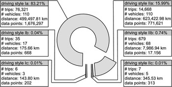
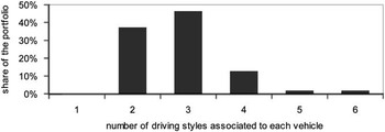
From the number of vehicles per driving style in Figure 12, which is in the sum overall styles considerably greater than the total number of vehicles in the whole telematic portfolio, it is clearly evident that trips of the same vehicle are not necessarily solely attributed to one driving style. This means that the driving behaviour of several different trips with the same vehicle may result in differently attributed driving styles. Figure 13 shows that the trips of each vehicle belong to at least two driving styles, the trips of 62.7% of all vehicle even covers between three and six different driving styles. This particularly illustrates that indeed driving style differentiation can be achieved under empirical real-world conditions. Moreover, the fact that more than half of all vehicles show trips in at least one of the supposedly less defensive driving styles. The reasons for this are switching drivers and routes with different traffic load as well as local conditions and inconsistent driving behaviour in itself. Even though the classification is performed with statistical foundation and still without risk assessment, one initial, general observation for the pricing approach can be derived from these findings, namely that a discount on the premium must be the result of weighted evaluation of the driving styles.
Survey of the number of driving style matches per vehicle.
Overall, it turns out that the driving styles based on empirical data correspond well with the driving styles deduced from simulated driving profiles. We clearly observe that driving style acceleration medians as well as deceleration medians of simulation and empirical portfolio match closely for all driving styles (see Figure 14, Appendix B for a more quantitative listing)Footnote 19 . The good consistency of the results of the two data sets indicates that the used measures of central tendencies and dispersion, the median and interquartile range, sufficiently describe the distributions of driving behaviour for classification within the present technical realisation. Thus, the classification can be carried out on aggregate data which is important in two ways. First of all, we can reduce the total data volume before transfer and consequently minimise the costs associated with transfer and storage management. Also, this way we consider the national data protection norms of the German insurance industry, with regard to data minimisation and data avoidance.
Polygon match of acceleration and deceleration medians (upper layer: stochastic simulation; lower layer: empirical).

5. Conclusion
It is not very likely that the high complexity of the actuarial tariff table will allow incorporating variables of driving behaviour into the table so long as an insurer has not yet established a risk experience in respect of telematic data. In spite of that, the question whether sensor data-derived tariff factors are substitutes for conventional tariff factors does not arise. However, subsequent discounts on the premiums dependent on the driving behaviour are a temporary opportunity to incorporate initial insights to telematic data. Premium reduction, which have to be determined on the basis of official accident statistics so long as no risk experience exist, acts as a stimulus to consumers concluding a telematic policy in order to establish a risk experience so that over the long term, variables of driving behaviour can substitute for conventional tariff criteria. In the actual literature, several questions concerning the differentiation and evaluation of driving behaviour are not answered. Thus, this paper provides a basis for optimised short- to medium-term pricing including telematic data, presenting a classification of driving profiles. Selected driving styles, which arise when driving profiles are modelled using a stochastic simulation, are considered. This approach accounts for possible parameter ranges as well as interdependencies and exemplary focusses on velocity, acceleration and deceleration behaviour.
The analysis leads to three main findings for insurance companies, each concerning the automobile product development, generating innovations, the actuarial division, calculating tariffs and management, undertaking pricing decision. First, a systematic method is introduced for generating specific driving styles using a vehicle mobility model. By connecting the model results to empirical insurance telematic data, we submit verification that driving profiles could be attributed to the identified driving styles. These styles are plausible and comprehensive because, as shown, the simulation model reflects the wide range of individual characteristics of driving behaviour.
Second, the analysis of the empirical telematic portfolio illustrates that the measurement and evaluation of driving behaviour should focus on essential information and furthermore exploits the full potential of differentiation. In spite of the fact that present telematic data is still subject to unfinished detection procedures, it is clearly established how partially inconclusive and possibly inaccurate telematic data can still be used to gain insights as long as the relevant features, such as the distribution’s main parameters, can be inferred.
Third, the introduced method for analysing specific driving behaviour also shows how the classification of driving styles can be carried out on aggregate data, i.e. measures of central tendencies as well as dispersion, using only a few variables including their interdependencies. This specific result appears of particular importance in the context of national privacy protection, in particular, with regard to the prime principles of data minimisation and data avoidance be met by any telematic tariff as far as personal data is concerned.
With this in mind, some methodological and conceptual limitations should be taken into account in the interpretation of our results. The driving styles shown here should only serve as an example, encouraging the extensive use of statistical methods as a basis for analysis of driving behaviour. Although we selected detailed model data in our analysis, other empirical portfolio-specific parameter sets should be applied to complete the picture. The verification of the model results should also be replicated with real-world telematic data sets of different composition of portfolio and data granularity in order to validate our findings. Moreover, it should be useful to extend the analysis by further data, in particular, variables of driving situation such as driving time or road conditions, which are far easier to analyse and can be approximated as conventional tariff criteria.
The results furthermore emphasise that the telematic risk assessment approach could have the potential for creative destruction in the matter of pricing innovation. The objective data on the individual usage of a vehicle provide new information in actuarial decision making. Thus, this approach could prospectively create a new insurance pricing structure, more differentiated and individualised than before. Insurers who use it can more adequately price the actual risk and gain competitive advantage.
Appendix A: Vehicle Mobility Model
Before we can introduce the RWP model, we need to present a set of abstract axioms and rules of movement necessary to describe the vehicle behaviour as close to realistic traffic conditions as possible.
Axioms
-
– Time-discrete system. A driving profile is given by a sequence of movement vectors in time-discrete succession – in general, GPS-based position measurements are also of this format.
-
– Microscopic model. The movement patterns of individual vehicles are based on the specific driving behaviour of the vehicle driver as well as the technical properties of the vehicle itself. The granularity of the description thus must be chosen such that distinctions can be drawn on the level of individual driver–vehicle units.
-
– Stochastic process. The driver–vehicle units as well as the environmental conditions (weather, traffic jams, resting times) are of stochastic nature.
Rules of movement
-
– Maximum velocity. The vehicle fits the individually desired velocity to the maximally allowed velocity. Limiting factors such as traffic density and road conditions and road type are included in the determination of the recommended speed, i.e. the velocity considered optimal under recognition of all external conditions.
This is of particular importance in Germany, where special conditions apply: on the Autobahn highways, there is not necessarily a speed limit, but rather a speed recommendation (Richtgeschwindigkeit) of 130 km/h. This means that in principle, the driver can exceed this velocity. The model accounts for this effect by weighting the deviation from the maximum speed less strictly if it is a recommendation instead of a limit. The model thus captures driving behaviour in countries with and without strict speed limits.
-
– Acceleration/deceleration behaviour. Vehicles do not start and stop without transition. We decompose the route between waypoints into segments of constant acceleration, so that the vehicle will accelerate at an individual rate at the beginning of the route until it moves with the segment-specific maximum velocity and decelerates at the end, each process conditioned on the type of waypoint in question.
-
– Stop times. At traffic obstacles like traffic lights, zebra crossings or traffic jams, the vehicle waits for a specific, stochastic waiting time.
Simulation of movement
In essence, the RWP model describes the movement of a driver-vehicle unit in a flat, bounded rectangle $[0,a]{\times}[0,b]\,\subset\,{\Bbb R}^{2} $
(see Bettstetter et al., Reference Bettstetter, Hartenstein and Pérez-Costa2004). The spatial distribution of all possible waypoints P=(P
x
, P
y
) is then uniformly distributed. For each simulated driver-vehicle unit (i.e. a so-called RWP node) j, j=1, 2, 3, … , m, a RWP P
0
(j) is chosen at the start of the simulation, then a sequence of waypoints P
i
(j),
$[0,a]{\times}[0,b]\,\subset\,{\Bbb R}^{2} $
(see Bettstetter et al., Reference Bettstetter, Hartenstein and Pérez-Costa2004). The spatial distribution of all possible waypoints P=(P
x
, P
y
) is then uniformly distributed. For each simulated driver-vehicle unit (i.e. a so-called RWP node) j, j=1, 2, 3, … , m, a RWP P
0
(j) is chosen at the start of the simulation, then a sequence of waypoints P
i
(j), $i\in{\Bbb N}$
, is selected from the restricted area. The movement of each node j consequently can be given as a time-discrete process:
$i\in{\Bbb N}$
, is selected from the restricted area. The movement of each node j consequently can be given as a time-discrete process:
 $$\left\{ {P_{i}^{{(j)}} } \right\}_{{i\,\in\,{\Bbb N}_{0} }} \,{\equals}\,P_{0}^{{(j)}} ,P_{1}^{{(j)}} ,P_{2}^{{(j)}} ,\,\ldots\,$$
The RWP node movement between waypoints is modelled by a segment-specific nominal velocity, sampled from the uniform distribution over [v min, v max], where v min>0 and v max<∞, and a component v(r i,k ) unique to the node. Thus, the speed at point r i,k , k=0, 1, 2, … , n i , is given by
 $$v_{i} (r_{{i,k}} )\,{\equals}\,v_{i} \cdot v(r_{{i,k}} )$$
Essentially, these nominal parameters are given by speed limits, traffic density and environmental conditions, whereas the personal part v(r i,k ) depends on the specific types of driver and vehicle. In order to make this mechanism as realistic as possible, before each step a waiting time T p , i is sampled from the normal distribution given by t p,i ϵ[0,t p,max] with t p,max<∞. In total, the movement period of a node is given by the vector (p i−1, p i , v i (r i,k ), t p,i ).
Driving profiles
To create specific driving profiles from the sample data we represent the stochastic process of distances between succeeding waypoints by (see Bettstetter et al., Reference Bettstetter, Hartenstein and Pérez-Costa2004)
 $$\{ L_{i}^{{(j)}} \} _{{i\,\in\,{\Bbb N}}} {\equals}L_{1}^{{(j)}} ,L_{2}^{{(j)}} ,L_{3}^{{(j)}} ,\,\ldots\,$$
with
 $$L_{i}^{{(j)}} \,{\equals}\,\left\Vert {P_{i}^{{(j)}} {\minus}P_{{i{\minus}1}}^{{(j)}} } \right\Vert_{2} \,{\equals}\,\left( {\left( {P_{{x,i}}^{{(j)}} {\minus}P_{{x_{i} {\minus}1}}^{{(j)}} } \right)^{2} {\plus}\left( {P_{{y,i}}^{{(j)}} {\minus}P_{{y,i{\minus}1}}^{{(j)}} } \right)^{2} } \right)^{\!\!\!{1/2}} $$
. Keep in mind that the velocity between waypoints is in general not constant, such that the measurement frequency crucially determines the quality of the velocity profile. In order to obtain segments {s
i,k
(j), k=0, 1, 2, … , n
i
}, we decompose every instance l
i
(j), depending on the chosen measurement frequency. From equal-time-distance tupels (s
i,k
, v
i
(r
i,k
)), iϵℕ0, k=0, 1, 2, … , n
i
, we can then refine a velocity-position profile, where for waiting delays t
p,i
we need to add tupels of the form (0, 0). In practice, any details of the movement are captured precisely if the measurement frequency is high enough, because for lower frequencies, velocity changes happening below the time resolution of the measurement cannot be resolved. However, in order to recreate an approximate velocity profile, measurements can be used as (linear) interpolation values. Consequently, for the average velocity between measurements P
i−1 and P
i
we find that
$$L_{i}^{{(j)}} \,{\equals}\,\left\Vert {P_{i}^{{(j)}} {\minus}P_{{i{\minus}1}}^{{(j)}} } \right\Vert_{2} \,{\equals}\,\left( {\left( {P_{{x,i}}^{{(j)}} {\minus}P_{{x_{i} {\minus}1}}^{{(j)}} } \right)^{2} {\plus}\left( {P_{{y,i}}^{{(j)}} {\minus}P_{{y,i{\minus}1}}^{{(j)}} } \right)^{2} } \right)^{\!\!\!{1/2}} $$
. Keep in mind that the velocity between waypoints is in general not constant, such that the measurement frequency crucially determines the quality of the velocity profile. In order to obtain segments {s
i,k
(j), k=0, 1, 2, … , n
i
}, we decompose every instance l
i
(j), depending on the chosen measurement frequency. From equal-time-distance tupels (s
i,k
, v
i
(r
i,k
)), iϵℕ0, k=0, 1, 2, … , n
i
, we can then refine a velocity-position profile, where for waiting delays t
p,i
we need to add tupels of the form (0, 0). In practice, any details of the movement are captured precisely if the measurement frequency is high enough, because for lower frequencies, velocity changes happening below the time resolution of the measurement cannot be resolved. However, in order to recreate an approximate velocity profile, measurements can be used as (linear) interpolation values. Consequently, for the average velocity between measurements P
i−1 and P
i
we find that
 $$\bar{v}_{i} \,{\equals}\,{{\mathop{\sum}\nolimits_{k\,{\equals}\,1}^{n_{i} } {s_{{i,k}} } } \over {\mathop{\sum}\nolimits_{k\,{\equals}\,1}^{n_{i} } {t_{{i,k}} } }},\,i\,\in\,{\Bbb N}$$
where t i,k is the time for the segment s i,k . Now if the measurement frequency is good enough, we can simplify the expression by taking t i,k =1/t A
 $$\bar{v}_{i} \,{\equals}\,{1 \over {n_{i} }}\,{\rm {\asterisk}}\,t_{A} {\rm {\asterisk}}\mathop{\sum}\limits_{k\,{\equals}\,1}^{n_{i} } {s_{{i,k}} ,\,i\,\in\,{\Bbb N}} $$
The acceleration profile naturally emerges from the first-order derivative of the velocity profile as $a_{i} (r_{{i,k}} )\,{\equals}\,\dot{v}_{i} (t,r_{{i,k}} )\,,\,i\in{\Bbb N}_{0} $
, k=0, 1, 2, … , n
i
. The average acceleration is then given by
$a_{i} (r_{{i,k}} )\,{\equals}\,\dot{v}_{i} (t,r_{{i,k}} )\,,\,i\in{\Bbb N}_{0} $
, k=0, 1, 2, … , n
i
. The average acceleration is then given by
 $$\bar{a}_{i} \,{\equals}\,{{v_{{i,m_{i} }} {\minus}\,v_{{i,l_{i} }} } \over {\mathop{\sum}\nolimits_{k\,{\equals}\,l_{i} }^{m_{i} } {t_{{i,k}} } }}\,,\,i\,\in\,{\Bbb N}$$
where $v_{{i,m_{i} {\minus}1}} \,\lt\,v_{{i,m_{i} }} \geq v_{{i,m_{i} {\plus}1}} $
and
$v_{{i,m_{i} {\minus}1}} \,\lt\,v_{{i,m_{i} }} \geq v_{{i,m_{i} {\plus}1}} $
and $v_{{i,l_{i} {\minus}1}} \geq v_{{i,l_{i} }} \,\lt\,v_{{i,l_{i} {\plus}1}} $
for a>0 or
$v_{{i,l_{i} {\minus}1}} \geq v_{{i,l_{i} }} \,\lt\,v_{{i,l_{i} {\plus}1}} $
for a>0 or $v_{{i,m_{i} {\minus}1}} \,\gt\,v_{{i,m_{i} }} \leq v_{{i,m_{i} {\plus}1}} $
and
$v_{{i,m_{i} {\minus}1}} \,\gt\,v_{{i,m_{i} }} \leq v_{{i,m_{i} {\plus}1}} $
and $v_{{i,l_{i} {\minus}1}} \leq v_{{i,l_{i} }} \,\gt\,v_{{i,l_{i} {\plus}1}} $
for a<0, respectively.
$v_{{i,l_{i} {\minus}1}} \leq v_{{i,l_{i} }} \,\gt\,v_{{i,l_{i} {\plus}1}} $
for a<0, respectively.
Parameters of the vehicle mobility model.

Appendix B: Quantitative Characterisation of the Driving Profiles
Frequency distribution of acceleration process.

Frequency distribution of deceleration process.

Frequency distribution of velocity process.


