


The community has played a key role in how scholars understand the crime problem for over a century. As we detailed in Chapter 2, the importance of community in understanding crime can be traced to the Chicago School, which saw the community as a key predictor of crime through the norms and circumstances that typified different neighborhoods. At least since the work of Shaw and McKay (1942 Reference Shaw and McKay1969]) criminologists have defined inner-city neighborhoods as “delinquency areas” and have assumed that there are strong differences across neighborhoods in a city in terms of crime levels, but relative homogeneity within neighborhoods (Cullen, Reference Cullen2018; Sampson, Reference Sampson, Wilson and Petersilia2011). As we noted in Chapter 1, recent research on hot spots of crime challenges this idea by showing that crime is highly concentrated, and that even within so called highcrime areas, most streets are relatively free of crime (Andresen and Linning, Reference Andresen and Linning2012; Weisburd, Reference Weisburd2015; Weisburd et al., Reference Weisburd, Groff and Yang2012; Zastrow, Reference Zastrow2021). In this sense, recent scholarship has pointed to the importance of focusing in on crime hot spots, rather than larger areas such as neighborhoods, when trying to address the crime problem. Much of the action of crime is at a very local level, defined in our work as street segments (Schnell et al., Reference Schnell, Braga and Piza2017; Steenbeek and Weisburd, Reference Steenbeek and Weisburd2016).
Acknowledging that crime is highly concentrated in cities and that there is strong street-by-street variability of crime even in areas that have overall higher levels of crime (Curman et al., Reference Curman, Andresen and Brantingham2015; Groff et al., Reference Groff, Weisburd and Yang2010; Weisburd et al., Reference Weisburd, Groff and Yang2012) still does not tell us whether differences between hot spots and non–hot spots vary between different types of communities, or whether crime hot spots themselves look different depending on the type of community they are located in. For example, it could be that the extent of concentrated disadvantage of hot spots is greater in high concentrated disadvantaged communities. Or it may be that hot spots evidence different levels of collective efficacy depending on the level of disadvantage of communities. The “delinquency area” perspective would suggest that the traits of streets would be strongly influenced by the characteristics of neighborhoods or communities. Hot spot perspectives on crime would suggest that such differences would be less important.
In this chapter, we go beyond a descriptive view of crime hot spots and how hot spots in a city differ from cold or cool spots, to explore how hot spots and non–hot spots vary within and across communities. Using the characteristics we focused on in Chapter 2 that evidenced significant variability between types of streets for our overall sample, we ask whether the extent to which hot spots and non–hot spots differ depends on the type of community they are nested within. We also examine to what extent hot spot streets have similar characteristics across the city, or whether hot spots look different depending on the community they are nested within. These questions are key to understanding the interplay between communities and crime hot spots.
3.1 Defining Types of Communities
A key question for us in developing our analyses was how to define communities in some way that we could compare them. The Baltimore City Department of Planning and Baltimore Data Collaborative divided the city of Baltimore into fifty-five Community Statistical Areas (CSAs) to be more consistent with perceived neighborhood boundaries. They followed four guidelines in constructing CSAs: (1) the boundaries had to align with Census Tracts, (2) consist of 1–8 tracts with populations ranging from 5,000 to 20,000, (3) define relatively homogenous areas, and (4) reflect the boundaries of communities recognized by city planners, institutions, and residents (Baltimore Neighborhood Indicators Alliance, 2018). The CSAs are frequently used in social planning, tracking city conditions and demographic trends, and are commonly employed in community research across various disciplines (e.g., see, Gomez, Reference Gomez2016; Kuen et al., Reference Kuen, Weisburd, White and Hinkle2022; Merse et al., Reference Merse, Buckley and Boone2008; Weisburd et al., Reference Weisburd, White and Wooditch2020).
We benefited from the fact that the Baltimore Neighborhood Indicators Alliance – Jacob France Institute (BNIA-JFI) aggregates census data at the tract level to Community Statistical Areas (CSA). Accordingly, we could use census information on the characteristics of the CSAs to define them into broad categories. Following the importance of social disorganization theory to our work, and the available data from the census, we decided to use concentrated disadvantage to broadly categorize the CSAs in Baltimore, since it is very much linked to structural indicators of social disorganization. (see Sampson, Reference Sampson2012; Wickes and Lanfear, Reference Wickes, Lanfear, Oberwittler and Wickes2025).
At the CSA level, our measure of concentrated disadvantage was estimated with a factor score approach, which included the percentage of Black residents, the percentage of families living below the poverty line, the unemployment rate, the percentage of female headed-households, the percentage of families receiving public assistance, and the percentage of individuals with less than a high school diploma.Footnote 1 In this sense concentrated disadvantage allows us to identify the extent to which CSAs differ by levels of social disorganization. Many other scholars have also taken this approach (e.g., see Jones and Pridemore, Reference Jones and Pridemore2019; Sampson, Reference Sampson2012; Sampson and Raudenbush, Reference Sampson and Raudenbush1999; Sampson et al., Reference Sampson, Raudenbush and Earls1997).
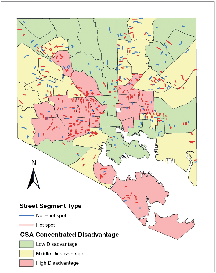
In Figure 3.1, the CSAs are overlaid on the city map of Baltimore with the streets in our study coded according to whether they are hot spots or non–hot spots (including “cold” or “cool spots”). Since we did not originally sample from CSAs as a sampling stratum, but rather from type of street segment, there are two CSAs that did not have any of our sampled streets, and a number with just a small number of sampled streets from the study. While this reflects our sampling approach, it means more generally, that we must find some overall way of characterizing the community areas if we want to draw inferences about the relationship between communities and crime hot spots.
Map of sample street segments by crime type within types of communities by concentrated disadvantage
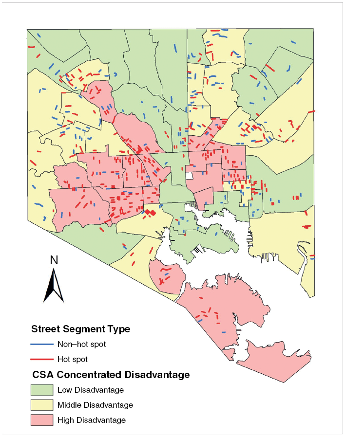
To allow for enough hot spots in each type of community for comparison, we divided the CSAs into low, middle, and high levels of concentrated disadvantage (see Sampson, Reference Sampson2012). This was done by simply placing the communities into three categories that roughly divide the sample by thirds from high to low: the top 34% (N = 18), the middle 34% (N = 18), and the bottom 32% categories (N = 17). Figure 3.1 shows the CSAs color coded by the type of community based on concentrated disadvantage. Many of the most disadvantaged CSAs surround the downtown, Inner Harbor of the city, reflecting Park and Burgess’s (Reference Burgess, Park and Burgess1925 [1967]) transitional zone characterized by disorganization that surrounded the central business district. The neighborhoods farer away from the center of the city are more likely to be in the low concentrated disadvantage group. Additionally, a characteristic unique to Baltimore termed the Black Butterfly by Professor Lawrence T. Brown, based on historically segregated communities is also evident in our map, with the spread of disadvantaged communities to the east and west of the inner harbor portraying wing-like shapes (Brown, Reference Brown2022).
Figure 3.1 also shows the street segments in our study coded by hot spots and non–hot spots. In the analyses below, we do not distinguish between the different types of hot spots, or between cool and cold spots because the samples would become too small for meaningful analyses within the three types of communities that we examine. But as we have already illustrated in Chapter 2, the general distinction between hot spots and non–hot spots is often a meaningful one for distinguishing streets in our study.
3.2 Looking More Closely at Hot Spots and Non–Hot Spots within the Same Communities
Before turning to our analyses comparing hot spots and non–hot spots across different community types, it is important to illustrate more directly the mixture of hot spot and non–hot spot streets within communities in our study sample. Sociological perspectives on crime in communities have often focused on units such as delinquency areas and emphasized the homogeneity of crime levels within such areas (Sampson, Reference Sampson, Wilson and Petersilia2011, Reference Sampson2012; Shaw and McKay, Reference Shaw and McKay1942 [1969]). Our work builds on studies that have emphasized the variability of crime levels on streets within communities and neighborhoods (Curman et al., Reference Curman, Andresen and Brantingham2015; Groff et al., Reference Groff, Weisburd and Yang2010; O’Brien, Reference O’Brien2019; Weisburd et al., Reference Weisburd, Groff and Yang2012).
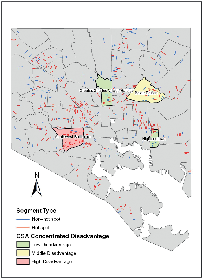
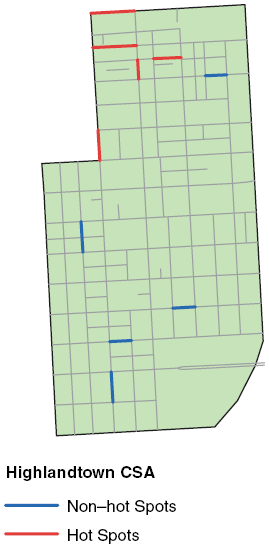
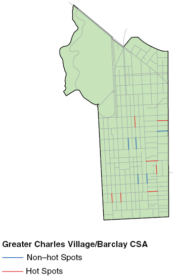
In forty-seven of the fifty-three CSAs in which we have sampled street segments, there are both hot spot and non–hot spot streets. Below we highlight four CSAs that provide illustrations of the presence and relative proximity of hot spots and non-spots within our sample across high, middle, and low concentrated disadvantage communities (see Figure 3.2). At the outset, it is important to keep in mind that our sample only includes a small percentage of streets in the city (449 street segments out of 25,045 in the city overall). Accordingly, the reality of mixture in the population is much greater than we show here.Footnote 2 In turn, a criterion for inclusion in our sample was that a street segment is not contiguous to other street segments (see the discussion on sampling in Chapter 1). Therefore, while the maps below show a realistic view of the city in which hot and non–hot spot streets are found within the same communities and often very close to each other, absent our sampling approach, the proximity of hot and non–hot spot streets would be even more pronounced.
Map of four CSAs at different disadvantage levels with hot spots and non–hot spots
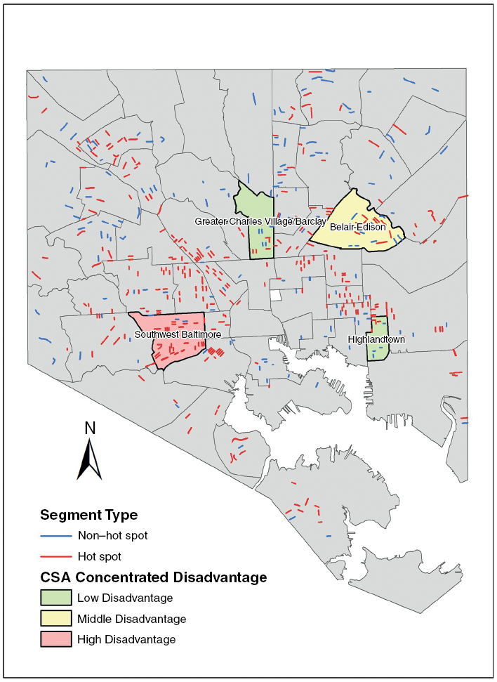
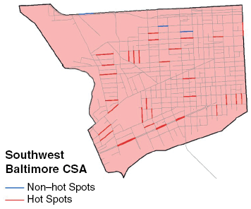
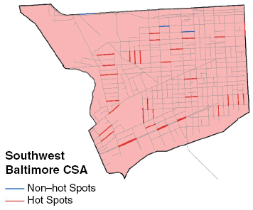
Southwest Baltimore (see Figure 3.3) is a high concentrated disadvantage community also known for high levels of crime. In 2012, the violent crime rate in Southwest Baltimore was 24.8 crimes per 1,000, and for all Part 1 crimes it was 76 crimes per 1,000, compared to the city, which registered 14.7 violent crimes per 1,000 and 61.8 Part 1 crimes per 1,000. Additionally, the number of calls to the police for shootings was nearly three times as high in Southwest Baltimore compared to the city overall (6.2 calls per 1,000 compared to 2.4 per 1,000), and narcotics calls were 244.1 per 1,000 compared to 89.7 per 1,000 for the city. In regard to our study, 31 hot spots from our sample were located in this CSA. Nonetheless, there were also three non–hot spots in our sample nested in this community. Note that two of these non–hot spots were within one block of hot spots in the CSA.
Map of Southwest Baltimore (high disadvantage community)
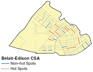
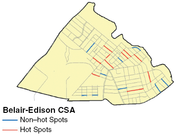
This interspersion of hot spots and non–hot spots is even more apparent in an example of a middle-level concentrated disadvantage neighborhood called Belair-Edison (see Figure 3.4). Belair-Edison had a violent crime rate of 14.9 crimes per 1,000, more aligned to the city-wide rate of 14.7 per 1,000. The crime rate for all Part 1 crimes was 52.7 per 1,000, the number of calls for shootings was 2.2 per 1,000, and narcotics calls were 53.9 per 1,000. In this CSA, we have a more balanced mixture of hot spots and non–hot spots in our sample, with 9 non–hot spots and 10 hot spots. While there is greater concentration of the hot spots in the center of the CSA, hot spots and non–hot spots are interspersed throughout.
Map of Belair-Edison (middle disadvantage community)
We can again see the mixture of hot and non–hot spots in a low-level concentrated disadvantage community, using the examples of Highlandtown on the east side of the city (see Figure 3.5), and Greater Charles Village/Barclay north of the city center (see Figure 3.6). Interestingly, despite these communities being lower in concentrated disadvantage, there still exists a great deal of crime. The violent crime rate in Highlandtown in 2012 was 20.8 crimes per 1,000 and the rate for all Part 1 crimes was 76.1 per 1,000, both much higher than the city rates; though calls for shootings and narcotics were lower than the city statistics, with 2.2 calls per 1,000 for shootings and 78.2 calls per 1,000 for narcotics. In the Highlandtown CSA, there are five non–hot spots and four hot spots in our sample.
Map of Highlandtown (low disadvantage community)
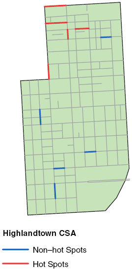
Map of Greater Charles Village/Barclay (low disadvantage community)
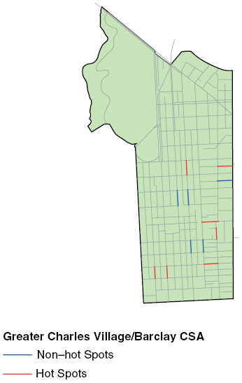
In Greater Charles Village/Barclay CSA (Figure 3.6), directly north of the city center, the violent crime rate was 16.2 crimes per 1,000, the crime rate for Part 1 crimes was 69.2 crimes per 1,000, the number of calls for shootings was 1.8 per 1,000, and the calls for narcotics was 59.2 per 1,000. There were five non–hot spots and twelve hot spots from our sample of street segments located in this CSA. In these maps, the presence of hot spots and non–hot spots close to each other is very apparent.
This closeness and interspersion of hot spot and non–hot spot streets was noted often in our qualitative interviews. One resident of a non–hot spot street in a low disadvantage community, for example, told us that “like any other city the streets vary “block by block” in terms of safety, drugs and crime.” Another resident of non–hot spot street also in a low disadvantaged community told us that in “places like Fells Point you might have one street where people are wealthy and going out or working downtown, and another street where women are on welfare with five kids live.” One resident of a non–hot spot in a middle disadvantaged community noted that his street “was still fine, but if you went a street over…” the areas were in “bad shape – they are dirty, have vacancies, and a lot of drugs and problems.” Similarly, a resident who lived on a hot spot located in a high disadvantaged community also commented on the variation across streets saying, “the neighborhood was generally safe, and it is more dangerous on other streets nearby, but not the one we’re on.”
These maps and qualitative passages provide only a few illustrations for the fact that hot spots and non–hot spots can be found within the same types of communities and even very close to each other. Again, our sample is only a small sample of all of the streets in these communities, and we purposely sampled so that streets would not be adjacent to each other. But even in our sample there is a good deal of mixture of hot spots and non–hot spots within the communities examined. More generally, these examples suggest the importance of recognizing the heterogeneity of crime within communities. Communities are not homogeneous in terms of crime levels, and though the extent of mixture varies, there are high-crime and low-crime streets within the different types of communities that we identify using concentrated disadvantage as a criterion.
3.3 Do Hot Spots and Non–Hot Spots Differ within Different Types of Communities?
Our first question is whether the type of community has strong influence on the relationship of hot spots to non–hot spots within communities. We found significant and consistent differences on a series of variables reflecting social structure and social context between hot spots and non–hot spots in Chapter 2 across our entire sample. Are those differences between hot spots and non–hot spots meaningful within high, middle, or low concentrated disadvantage communities? Or do differences vary greatly depending on the type of community that a hot spot is nested within? For example, does being located in a high disadvantage community seem to increase the disadvantages found in crime hot spots, or conversely do the advantages found in low concentrated disadvantage communities lessen the disadvantages that hot spots experience in these communities?
3.3.1 Structural Indicators of Social Disorganization
As we noted in Chapter 2, social disorganization theory links failures of social organization to social disadvantage found in specific urban neighborhoods in the city. Such areas, for example, were assumed to have high levels of concentrated disadvantage, leading to low levels of informal social control. We illustrated in Chapter 2 that structural indicators of social disorganization were strongly related to hot spots of crime. Does this relationship vary by type of community?
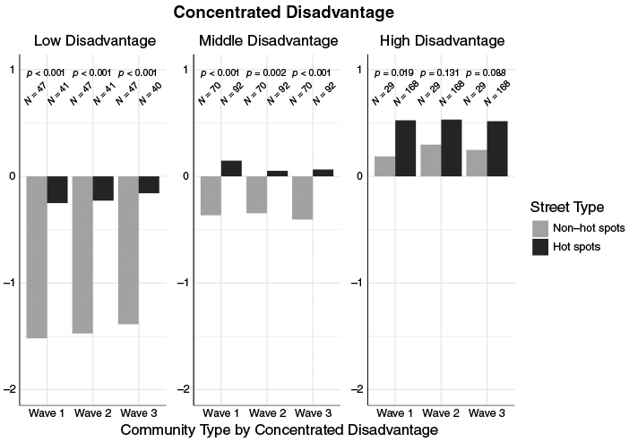
In Figure 3.7, we compare hot spots and non–hot spots in the three types of communities, as defined by concentrated disadvantage, across each of the three waves. What we see here is that in the middle and low disadvantage communities there are strong and significant differences (at least p ≤ 0.002) across each wave reflecting our general findings of much greater concentrated disadvantage in crime hot spots than non–hot spots. While the direction of the relationships is similar for the high disadvantage communities, the differences were only statistically significant in wave 1 (p < 0.05).
Concentrated disadvantage in hot spots and non–hot spots across different types of communities
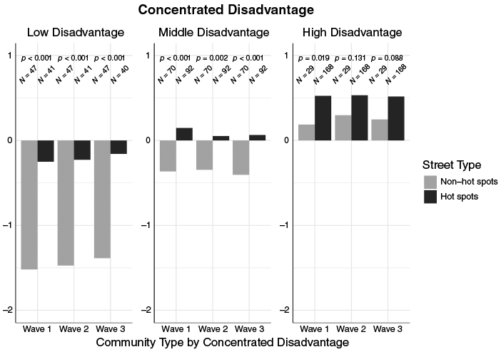
These findings suggest that the community context in which streets are located does moderate the differences observed between hot spot and non–hot spot streets. We suspect that these results are directly linked to the very high levels of concentrated disadvantage found in high disadvantaged communities. In these communities, both hot and non–hot spots have higher average levels of concentrated disadvantage – the values for non–hot spots across the three waves are all above zero on our scale, contrasting with the negative values for non–hot spot streets in middle and low disadvantage communities. In some sense, while crime hot spots across types of communities have higher levels of concentrated disadvantage than non–hot spots, these disadvantages are intensified both for hot spot and non–hot spot streets in high disadvantage communities. In these communities, the differences between hot spot and non–hot spot streets become less apparent, as both types of streets evidence relatively higher levels of concentrated disadvantage.
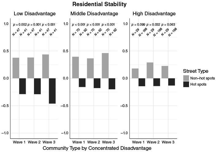
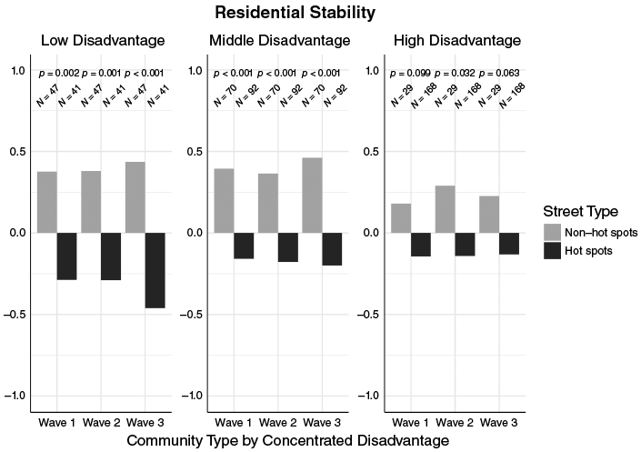
Another important structural indicator of social disorganization is residential stability. In Figure 3.8 we compare hot spots and non–hot spots across the three waves. Again, we find very strong and significant differences (at least p ≤ 0.002) for low and middle concentrated disadvantage communities, but more marginal findings for high disadvantage communities. Only in wave 2 are the differences statistically significant, while in waves 1 and 3 the differences were marginally significant (p < 0.10). This suggests again that the overall higher levels of social disorganization in high concentrated disadvantaged communities are reducing the degree of differences in residential stability between hot spots and non–hot spots.
Residential stability in hot spots and non–hot spots across different types of communities
3.3.2 Informal Social Control
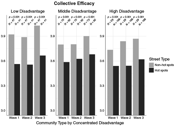
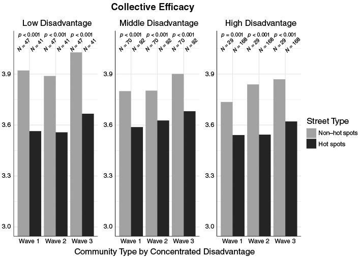
We emphasized the importance of collective efficacy in Chapter 2, and its direct representation of levels of informal social control in the community. As we noted there, the relationship between informal social control and crime has been a key part of criminological research since sociologists of the Chicago School coined the term ‘social disorganization’ in the 1920s to represent the degree to which neighborhoods were unable to exercise informal social control to prevent crime (Burgess, Reference Burgess, Park and Burgess1925 [1967]; Park and Burgess, Reference Park and Burgess1925; Shaw et al., Reference Shaw1929; Shaw and McKay, 1942 [Reference Shaw and McKay1969]). In Chapter 2, we showed that informal social control, measured as collective efficacy, varied strongly between hot spots and non–hot spots. Looking within types of communities, our findings are reinforced (Figure 3.9). In each type of community for each wave there are strong and significant differences (p ≤ 0.001) between hot spots and non–hot spots. Consistent with our findings in Chapter 2, across the city, hot spots of crime evidence much lower levels of informal social control as measured by collective efficacy irrespective of the type of community they are nested within.
Collective efficacy in hot spots and non–hot spots across different types of communities
3.3.3 Social and Physical Disorder
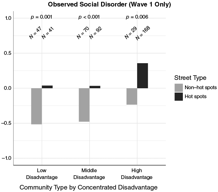
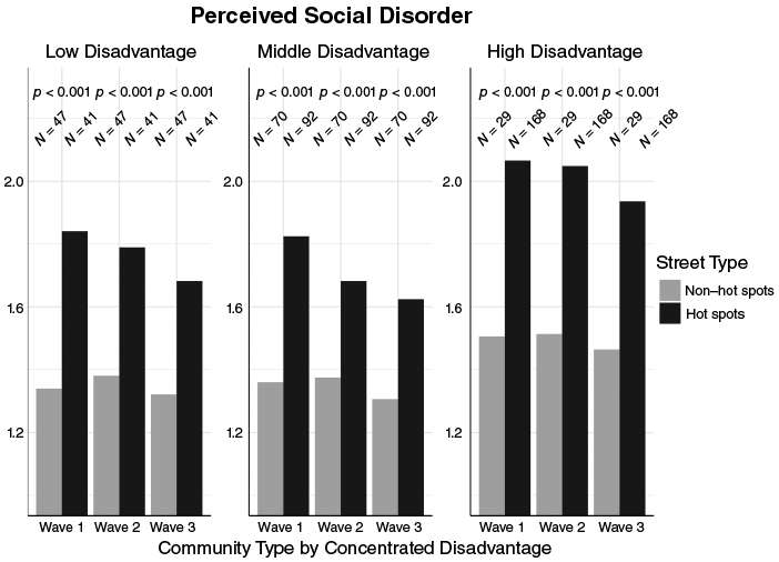
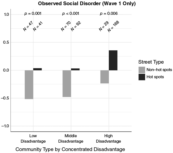
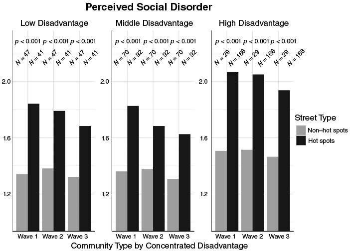
Based on our systematic social observations conducted in wave 1 of the study, within each type of community as defined by concentrated disadvantage, hot spots show significantly higher (at least p ≤ 0.006) levels of observed social disorder than non–hot spots (see Figure 3.10). This is true as well when we look at perceived social disorder from the residential survey (see Figure 3.11). Across all three waves and across all three types of communities, people who live on hot spot streets identify significantly (p < 0.001) higher levels of social disorder than people who live on non–hot spot streets. As we noted in Chapter 2, scholars have sometimes seen social disorder as similar to measures of crime (Sampson, Reference Sampson2012; Sampson and Raudenbush, Reference Sampson and Raudenbush1999; see also Gau and Pratt, Reference Gau and Pratt2008), and in this context, higher levels of social disorder on crime hot spots are not surprising. But again, it does indicate that people who live on crime hot spots are very much aware of such problems on their street.
Observed social disorder in hot spots and non–hot spots across different types of communities (wave 1 only)
Perceived social disorder in hot spots and non–hot spots across different types of communities
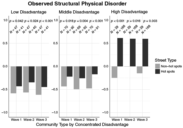
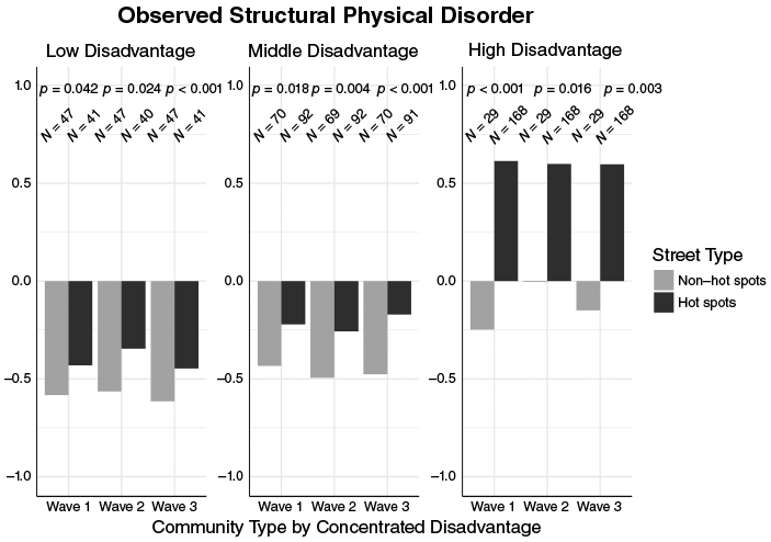
Our observed physical observation data and perceived physical disorder in our surveys also reinforce the fact that hot spots and non–hot spots differ greatly within each of the three types of communities as defined by concentrated disadvantage. As noted in Chapter 2, we focused on two main types of physical disorder in our observations of the streets: structural disorder and sidewalk disorder (see Table A2.1 for the full list of measures and factor analysis results). In all nine comparisons across waves and types of communities, the hot spots have much higher levels of physical disorder (see Figure 3.12, at least p < 0.05). In this regard, the levels of observed structural disorder on street segments, which include vacant lots, buildings with broken windows, and boarded-up buildings, are much higher in the high disadvantage communities.
Observed structural physical disorder in hot spots and non–hot spots across different types of communities
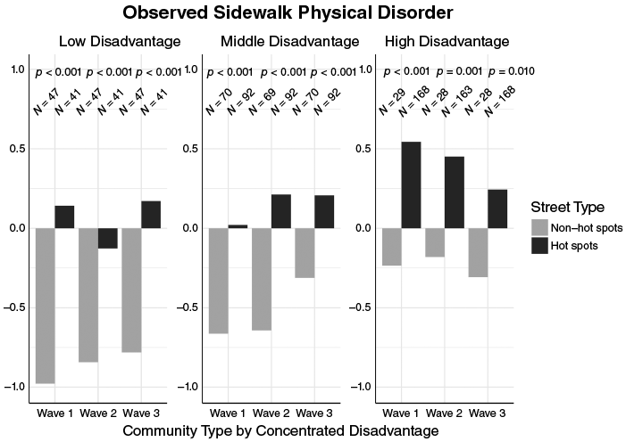
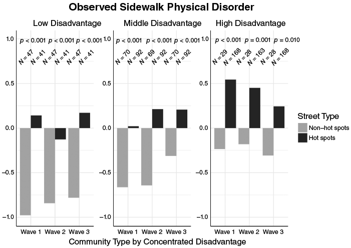
We also find significant differences (at least p < 0.05) across all three types of communities across all three waves for observed sidewalk disorder, which includes litter, broken bottles and glass, and cigarette and cigar butts on the streets (see Figure 3.13). The difference between hot spots and non–hot spots is particularly large and significant for the low and middle disadvantage communities (p < 0.001). Again, the levels of physical disorder are overall higher on average for both hot spots and non–hot spots in the high disadvantage communities, perhaps representing generally higher levels of disorder in those communities.
Observed sidewalk physical disorder in hot spots and non–hot spots across different types of communities
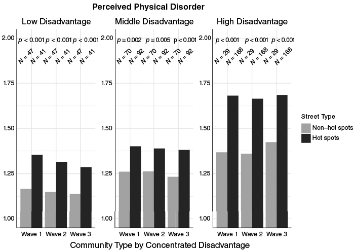
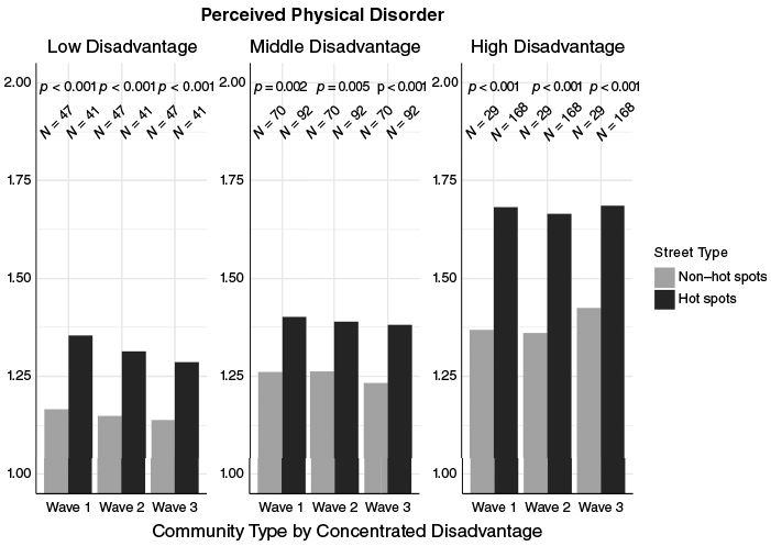
And these higher levels of physical disorder are also observed by people who live on these streets. Again, in all of the comparisons, we find that residents of hot spots perceive significantly higher levels (at least p < 0.01) of disorder compared to those of non–hot spots (see Figure 3.14).
Perceived physical disorder in hot spots and non–hot spots across different types of communities
3.3.4 Fear of Crime
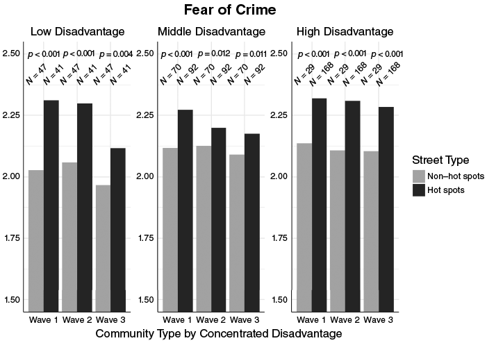
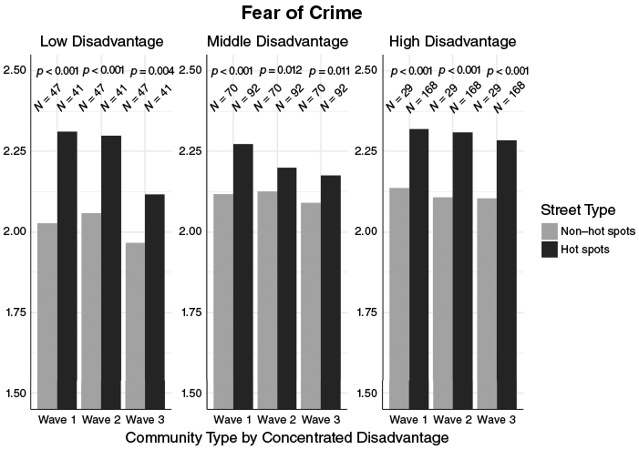
Fear of crime varies greatly across the three types of communities. Irrespective of the crime levels and actual risks of victimization within each community, there are significant (at least p < 0.05) and strong differences between hot spots and non–hot spots in fear of crime within each community type (Figure 3.15). Regardless of the type of community within which a hot spot is found, residents of hot spots are significantly more fearful of crime than those living on non–hot spot streets. The relationship is most consistent and significant (p < 0.001) across waves of the survey in the high disadvantage communities. Overall, our findings make sense given the high-crime levels found at crime hot spots, and to some degree emphasizes that people who live in these places are aware of the crime problems on their streets.
Fear of crime in hot spots and non–hot spots across different types of communities
What we have seen so far is that hot spots and non–hot spots are generally distinguished not only across the city but also within types of communities as defined by levels of concentrated disadvantage. At the same time, in specific comparisons, the community context clearly affects characteristics of crime hot spots. This is true especially for structural measures of social disorganization in high concentrated disadvantage communities, where we found that the distinctions between hot spots and non–hot spots are much smaller. Now we turn to a different question, which focuses on whether hot spots are similar in characteristics across communities.
3.4 Are Hot Spots Similar in Characteristics across Communities?
It is clear from our sampling approach that non–hot spots will closely reflect the communities that they are nested in. This is because most of the streets in the city are non–hot spots given our identification of hot spot streets as being in the top 3 percent of crime calls for drugs and violence in 2012. Accordingly, we would not learn much by examining whether non–hot spots differ across communities, because we already know that the communities they are nested in vary greatly, for example, in levels of concentrated disadvantage. But the question of whether characteristics of crime hot spots reflect the communities they are nested within, or seem to be independent of those communities, remains an important empirical question. The hot spots idea suggests that there is something common to hot spots across communities. At the same time, we have already seen that differences between hot spots and non–hot spots do sometimes vary depending on the communities that the streets are nested within.
3.4.1 Structural Indicators of Social Disorganization
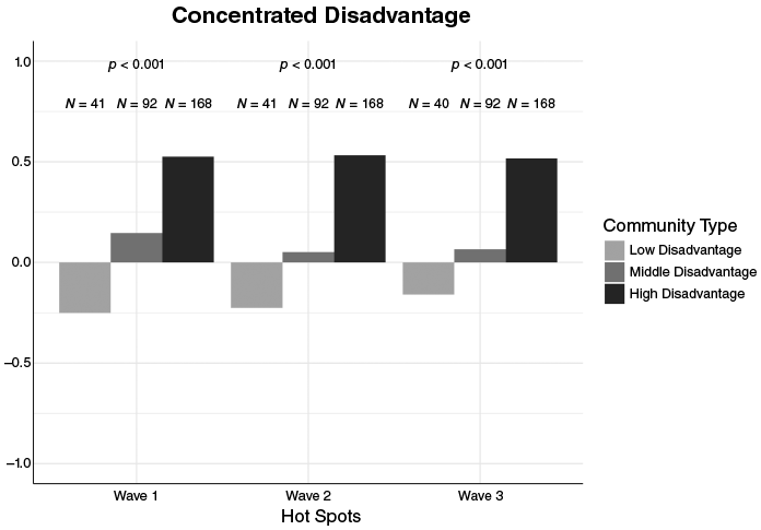
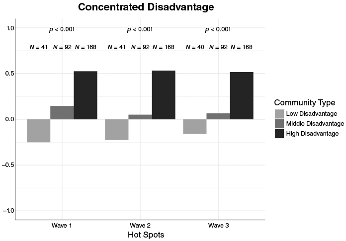
Beginning with concentrated disadvantage, it is clear that community type is significant in understanding structural characteristics of hot spots (p < 0.001). Levels of concentrated disadvantage across the three waves of the survey are higher in hot spots located in high concentrated disadvantage communities than in middle and low disadvantage communities (see Figure 3.16). Put simply, when a community faces high levels of concentrated disadvantage, then hot spots in those communities are likely to evidence higher concentrated disadvantage. This points to the importance of community in understanding structural features of social disorganization at specific hot spots. The higher levels of concentrated disadvantage on hot spot streets in high concentrated disadvantage communities suggests that hot spots in those communities suffer from additional disadvantages than hot spots in lower concentrated disadvantage communities.
Comparison of concentrated disadvantage at crime hot spots across different types of communities
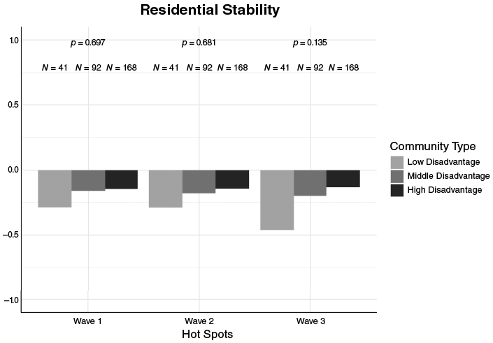
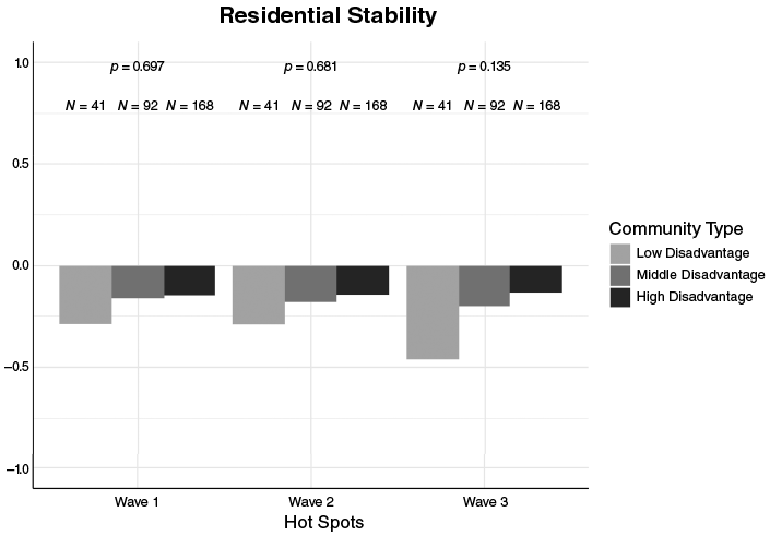
While the pattern of relationships for residential stability across the three types of communities in our samples is similar to that of concentrated disadvantage, the differences are not significant in any of the three waves (see Figure 3.17). This suggests that residential stability at crime hot spots is not meaningfully impacted by the type of community that a hot spot street is located within. Hot spots have low residential stability whether they are in high, middle, or low disadvantage communities, and those levels do not significantly differ within hot spots across communities.
Comparison of residential stability at crime hot spots across different types of communities
3.4.2 Informal Social Control
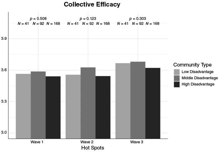
As we have noted before, direct measures of informal social control (in our study, collective efficacy) are perhaps the most important indicators of the ability of hot spot communities to play a role in controlling problems on the street. And here we find strong evidence that hot spots of crime are similar across different types of communities (see Figure 3.18). This suggests that the community may not be a major influence on informal social control at crime hot spots.
Comparison of collective efficacy at crime hot spots across different types of communities
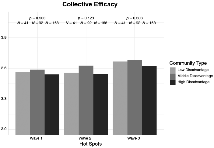
For hot spots, collective efficacy levels are similar across low, middle, and high concentrated disadvantage communities across the three waves of data. This finding illustrates very starkly the degree to which informal social control at crime hot spots is very much a consequence of the local influences on those streets, rather than the broader influences of the communities in which they are nested. Whether in a high disadvantage or low disadvantage community informal social controls at the hot spots of crime are remarkably similar. This points to the key importance of the immediate environment of the hot spots, as contrasted with the character of the community within which they are found.
3.4.3 Social and Physical Disorder
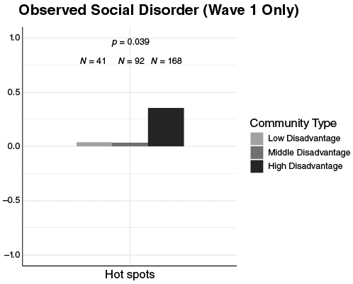
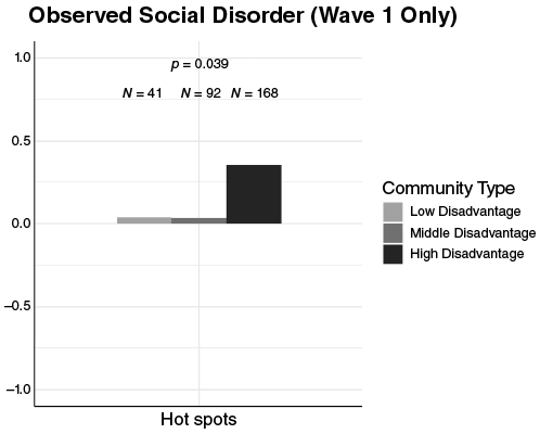
At crime hot spots, the systematic social observations of social disorder vary significantly across community type (p < 0.05). Hot spots in communities with high concentrated disadvantage have much higher levels of social disorder compared to those with low or middle disadvantage (p < 0.05; see Figure 3.19).
Comparison of observed social disorder at crime hot spots across different types of communities
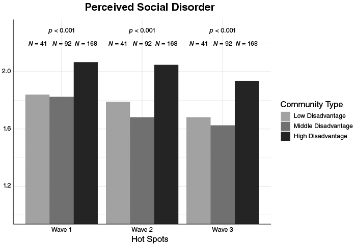
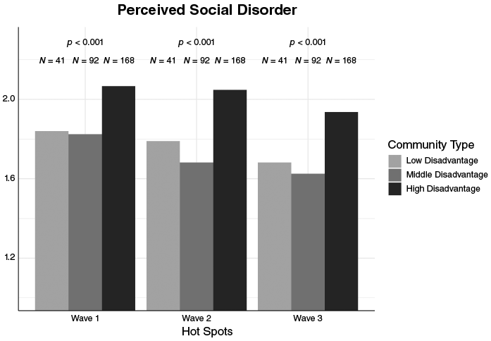
Turning to perceptions of social disorder (see Figure 3.20), there are significant differences between hot spots in the three types of communities (p < 0.001). But again, we observe little difference in terms of the hot spots in low and middle disadvantaged communities, and they tend to have residents observe about the same levels of social disorder on the street. However, perceptions of social disorder are much higher in each wave for hot spots in the high disadvantage communities.
Comparison of perceived social disorder at crime hot spots across different types of communities
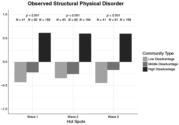
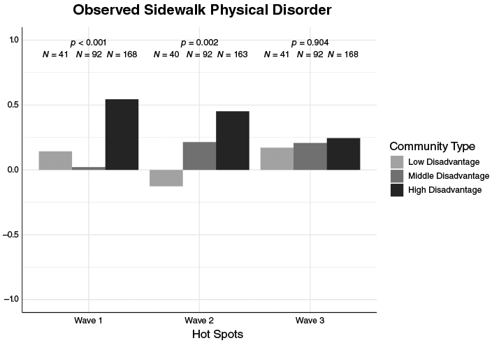
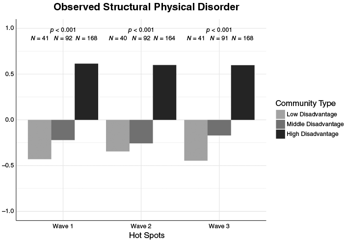
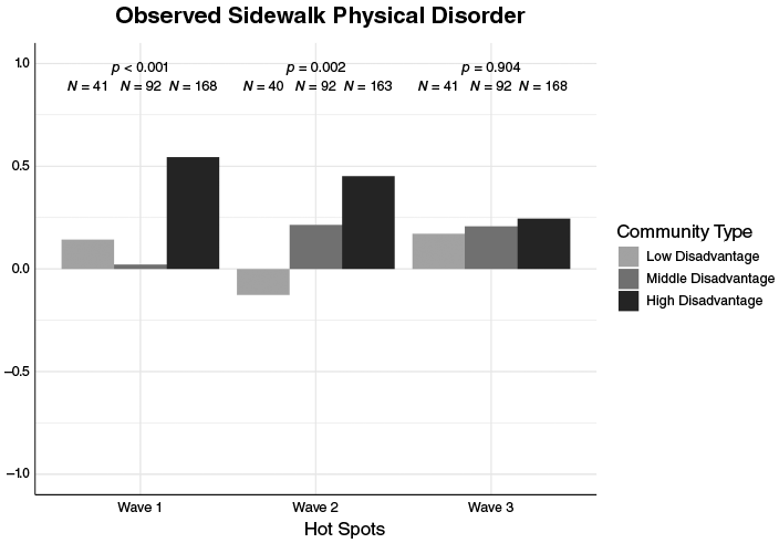
These findings are also reflected when we examine observed and perceived physical disorder. In terms of observed structural physical disorder (see Figure 3.21), crime hot spots in high disadvantage communities show higher levels of disorder compared to those in communities with low or middle disadvantage (p < 0.001). For observed sidewalk disorder (see Figure 3.22), similar results are found for wave 1 (p < 0.001) and wave 2 (p < 0.01). However, in wave 3 there are small and insignificant differences across the communities.
Comparison of observed structural physical disorder at crime hot spots across different types of communities
Comparison of observed sidewalk physical disorder at crime hot spots across different types of communities
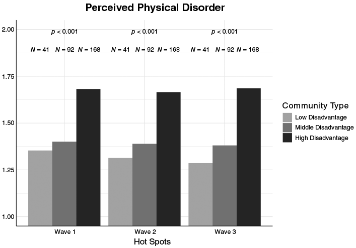
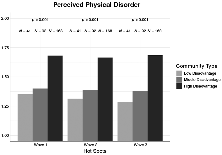
Community context again appears to be important in measuring perceived physical disorder across the three waves (see Figure 3.23). Residents of hot spots of crime in high concentrated disadvantage communities perceive higher levels of disorder than in middle or low disadvantage communities (p < 0.001). Together with our other disorder measures, we think that our data suggest that hot spots in higher disadvantage communities suffer from relatively higher levels of physical disorder, and residents on these hot spots recognize this.
Comparison of perceived physical disorder at crime hot spots across different types of communities
3.4.4 Fear of Crime
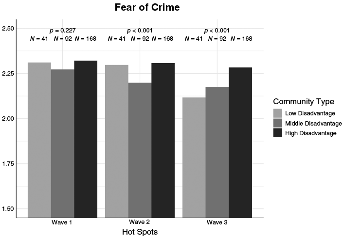
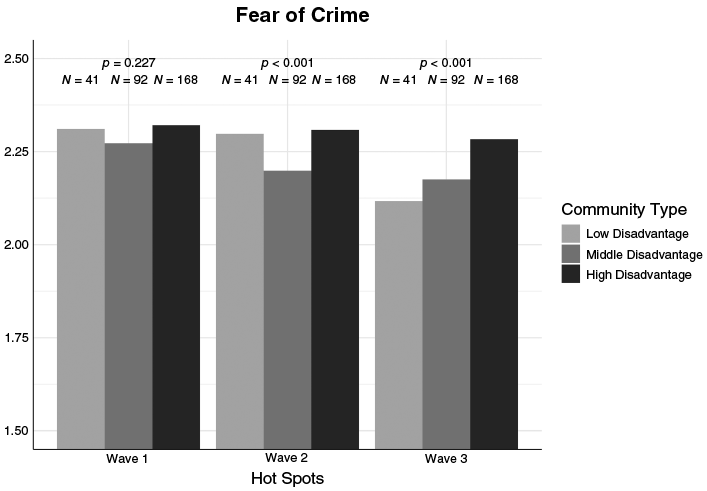
Fear of crime has inconsistent influences across the three waves (see Figure 3.24), though in the second and third waves, the differences between the three types of communities are statistically significant (p < 0.001). In wave 2, the hot spots in the middle disadvantage communities have the lowest level of fear, but in wave 3 this is true of the hot spots located in the low disadvantage communities. One explanation for this may be that in wave 2, as we noted in Chapter 1, the Freddie Gray riots occurred, and some of our surveys were done during or immediately after this period. We might expect that residents in low disadvantage communities would be particularly fearful of the riots and the lawlessness that was associated with the riots. The inconsistency of these findings across waves does not allow us to draw any strong conclusions regarding this measure.
Comparison of fear of crime at crime hot spots across different types of communities
3.5 Conclusions
We began this chapter by asking whether hot spots and non–hot spots differ within different types of communities, defined by their levels of concentrated disadvantage. The delinquency area perspective would predict a great deal of homogeneity within communities (Shaw and McKay, 1942 [Reference Shaw and McKay1969]; see also Sampson, Reference Sampson2012), while the hot spot perspective would predict variability between streets, especially when comparing hot spots and non–hot spots (Weisburd et al., Reference Weisburd, Groff and Yang2012). First, we illustrated that hot spots and non–hot spots in our sample are often found in the same communities, and often near to each other. This already suggests the heterogeneity of crime problems within communities, which has been illustrated in a series of prior studies (Curman et al., Reference Curman, Andresen and Brantingham2015; Groff et al., Reference Groff, Weisburd and Yang2010; Weisburd et al., Reference Weisburd, Groff and Yang2012). However, our purpose was to see whether other traits observed also show within community variability, and to what extent hot spots of crime are similar or different across communities.
Overall, we found that just as hot spots are differentiated from non–hot spots in the city overall, they are also distinguished within specific types of communities as defined by social disorganization. Whether we look at the concentrated disadvantage of streets, residential stability, informal social control, social disorder, physical disorder, and fear of crime, across the comparisons we examined, hot spots differ significantly from non–hot spots irrespective of which type of community they are found in. Put differently, there is tremendous variability within communities regarding the character of hot spot and non–hot spot streets. This points to the overall significance of hot spots of crime, irrespective of community character.
At the same time, our analyses point to the importance of community type for understanding differences between hot spots and non–hot spots in specific circumstances. In the case of our street measure of concentrated disadvantage, the difference between hot spots of crime and non–hot spots has much less salience and is often not statistically significant in high concentrated disadvantaged communities. We noted that this is likely related to the overall very high level of disadvantage in such communities in the first place. In high disadvantage communities in Baltimore, social disorganization is at a high level throughout those communities, and this affects both hot spots and non–hot spots. So, in these cases, the very strong differences we observe overall between hot spots and non–hot spots are more constrained. This suggests the importance of nuance in understanding the complex relationships between the broader communities hot spots are nested within and the micro-communities of the hot spots themselves (O’Brien, Reference O’Brien2024; see also O’Brien and Ciomek, Reference O’Brien and Ciomek2023). The hot spots perspective is confirmed in its emphasis on within community variability. However, community matters as well for specific characteristics, such as structural measures of social disorganization and disorder.
This nuance is further reflected when we examined the extent to which hot spots of crime differ across communities. Concentrated disadvantage of streets differs strongly for hot spots in communities with low, middle, and high concentrated disadvantage. Community here clearly has an influence, with hot spots in very high disadvantaged communities evidencing much higher levels of concentrated disadvantage than those located in low or middle level communities. These differences are also reflected when we look at observed and perceived physical and social disorder. Across several measures, it is clear that while hot spots of crime generally are more disorderly than non–hot spots, whether we look at social or physical disorder, such levels are significantly higher in the high disadvantaged communities. At least in terms of concentrated disadvantage and social and physical disorder at the street-segment level, community matters; when the community is of higher concentrated disadvantage, the hot spots will have relatively higher levels of disadvantage as well, as compared with hot spots in lower concentrated disadvantage communities.
Perhaps the most important finding in this chapter relates to the fact that our measure of informal social control for crime hot spots does not vary according to the communities they are found in. Despite the reinforced disadvantages we observed in terms of concentrated disadvantage and disorder in high disadvantaged communities, hot spots of crime have similarly lower levels of informal social control as measured by collective efficacy, irrespective of the type of community they are nested in. And these findings regarding collective efficacy are remarkably consistent. While we might expect collective efficacy at hot spots to be particularly low in high disadvantaged communities, collective efficacy varies little between hot spots located in high, middle, and low concentrated disadvantage communities. This suggests that informal social control on these streets is not strongly moderated by community context, or at least the elements of community context that concentrated disadvantage represents. This finding is reinforced when we examined residential stability. While the pattern of relationships in the sample shows higher residential instability for crime hot spots in high concentrated disadvantage communities, those differences are not large nor significant.

 Open access