
… their effects far exceed any effects likely to occur from global climate change over a period of several centuries.
As noted earlier, a variety of conditions will control the response on different rivers.
4.1 Hydraulic Infrastructure and Society
4.1.1 Context and Focus
Many rivers are substantially degraded because of human reliance upon water resources to support intensive agriculture, industry, and settlement. This includes emplacement of “hard engineering” structures that modify landscapes and water supplies, such as dams, dikes (levees), groynes, river bank protection, and irrigation networks, among other forms.
Dams and reservoirs are a specific type of hydraulic infrastructure constructed to meet a variety of societal demands and provide stable water supplies for irrigation, navigation, industry, flood control, enabling agricultural activities and human settlement to expand upon marginal lands (Williams and Wolman, Reference Williams and Wolman1984; Graf, Reference Graf2006). Dams and reservoirs, however, have many unintended adverse consequences. These include altered hydrologic regimes and sediment trapping that impact downstream environments, and in some cases increase human vulnerability to global environmental change. Additionally, constructing dams to reduce flood risk is a false justification. This is because flood control results in reduced downstream flow variability for the purpose of promoting floodplain development for settlement and agriculture within a predictable physical environment, which is the actual justification.
This chapter singularly focuses on dams, the major form of hydraulic infrastructure in the upper and middle reaches of drainage basins, and which impact downstream fluvial lowlands and deltas. The chapter begins by examining the motivation for dam construction and establishes their near ubiquitous presence upon the global riparian landscape. Next, the environmental impacts of dams are systematically reviewed, including hydrologic, sedimentary, geomorphic, and ecological impacts. While some nations are experiencing a surge in dam construction, others are practicing dam removal, which holds great potential to restoring downstream environments. Many dams, however, are effectively permanent components of the riparian environment (Figure 4.1), which behooves government organizations to develop strategies for sustainable management of reservoir sediments. While some dams are constructed in the lower portions of drainage basins, hydraulic infrastructure in lowland floodplains and deltas primarily consists of flood control dikes and hard structures to stabilize rivers in support of navigation. These forms of hydraulic infrastructure are systematically examined in subsequent chapters (Chapters 5, 6, and 7), including environmentally progressive approaches within the framework of integrated river basin management (Chapter 8).
Red Bluff Diversion Dam on Sacramento River, California, constructed from 1962 to 1964 (closure) to support 61,000 ha of irrigated agriculture for massive Central Valley Project (decommissioned in 2013 for environmental reasons), supplied by two large irrigation canals (photo).

4.1.2 Dams, Agriculture, and Water Resources
Hydraulic societies were ancient agrarian civilizations organized around water resource management by robust government institutions, as originally described by Wittfogel (Reference Wittfogel1957). Historically, the concept applied to lowland rivers in Mesopotamia, eastern China, the lower Indus, the Nile in Egypt (see Butzer, Reference Butzer1976; Wolman and Giegengack, Reference Wolman, Giegengack and Gupta2007), as well as pre-Columbian societies in the Americas (see Denevan, Reference Denevan2000; Doolittle, Reference Doolittle2000; Mann, Reference Mann2005). The concept of hydraulic societies reinforces the point that – because of their extensive size and sophistication of design – hydraulic infrastructure along large rivers require well-functioning government institutions for planning, construction, and management and maintenance. This was true for ancient societies, and as we’re constantly reminded, remains valid today.
Global freshwater withdrawals have increased greatly since 1900 and especially after the 1950s (Figure 4.2). Some 70% of global freshwater withdrawals are to support agriculture. And because of reservoir evaporation, the actual percentage of global freshwater withdrawals could be closer to ~80%, as many reservoirs in dry regions were historically constructed to support agriculture and have high rates of evaporation. For societies heavily dependent upon riverine freshwater resources, evaporative losses can be a substantial component of the annual water budget, increasing vulnerability to water scarcity caused by climatic fluctuations or upstream political rivals. The evaporation rate at Lake Nasser and Lake Nubia, the massive 5,275 km2 reservoir that impounds the Nile River upstream of the Aswan High Dam in Egypt and Sudan, ranges from an average daily maximum in June of 10.9 mm/day to an average daily minimum in January of 3.8 mm/day. The amount of Nile River water lost by evaporation in Lake Nasser ranges from 10 to 16 billion m3/yr. While the Nile River supplies Lake Nasser with 55 billion m3/yr, evaporation results in a loss of 18–29% of annual totals (El Bakry, Reference El Bakry1994; FAO, 2016; El-Mahdy et al., Reference El-Mahdy, Abbas and Sobhy2019). Within such a hyperarid region this constitutes a substantial loss of freshwater, and increases downstream water stress for riparian agricultural stakeholders.
Global water withdrawals by sector since 1900, showing steep increase after the 1950s.

Many dams exist as part of a larger agricultural system that requires stable freshwater supplies from extensive irrigation networks. Indeed, irrigation networks necessitate additional forms of engineering structures, including weirs, sluices, pumps, ditches and canals to distribute water between reservoirs and fields (Figure 4.1). Thus, the riparian impact of dams is very much part of a broader impact of agriculture on the environment. The Mekong basin, for example, receives considerable attention because of the recent boom in dam construction for hydropower. But already the impact of agriculture on water resources across the Mekong basin is extensive (Hortle and Nam, Reference Hortle and Nam2017). Irrigation projects in the Mekong basin include an extensive amount of hydraulic infrastructure for support, including 5,366 dams and reservoirs, 2,454 weirs (low-flow dams), 2,469 pumps, and 278 sluices (Table 4.1). Paradoxically, to ensure regional food security because of projected losses to inland Mekong River fisheries caused by intensive dam construction for hydropower, an increase in agricultural lands of 19–63% is required, which includes dam construction to support irrigation networks (Pokhrel et al., Reference Pokhrel, Burbano, Roush, Kang, Sridhar and Hyndman2018).
* As registered on the DMFPF project of the Mekong River Commission’s Agriculture, Irrigation and Forestry Project in 2003.
** Built by the French under colonial system for the purpose of transporting silty river water over natural levees into backswamp to build up agricultural lands (see Dennis, Reference Dennis, Ablin and Hood1990; FAO, 2011a).
The hundredth meridian in North America has special importance as it relates to water resources. This is because it broadly corresponds to the 50 cm isohyet of annual precipitation, and signifies the boundary between agriculture supported by rainfall versus agriculture supported by water supplied by irrigation networks (Powell, Reference Powell1895; Stegner, Reference Stegner1954). The climatic significance of the hundredth meridian is that it represents the approximate westerly limit of humid tropical moisture supplied from the Gulf of Mexico (Seager et al., Reference Seager, Lis and Feldman2018). Much of the land beyond the hundredth meridian effectively lies in the rain shadow of the mountain west and basin and range region, requiring considerable hydraulic infrastructure to support agriculture. Of course, beginning in the late nineteenth century, and prior to the development of numerous dams and irrigation networks west of the hundredth meridian (Reisner, Reference Reisner1993 [1986]), the western Great Plains were already being developed and cultivated based on a flimsy scientific posit known as “rain follows the plow,” which was especially pushed by land speculators to encourage westward development (Smith, Reference Smith1947; McLeman et al., Reference McLeman, Dupre, Ford, Ford, Gajewski and Marchildon2014). The idea was that, following the onset of agriculture in dry regions, rainfall would increase because high evapotranspiration rates from crops would produce summer cloud bursts to satiate thirsty lands. This nonsensical and dangerous contention placed agriculture and human settlement at an environmental tipping point, one that was dramatically exceeded in the dry decade of the 1930s, the era of the American Dust Bowl. Unfortunately, the concept was exported to dry southeastern Australia, within the Murray River basin as farmers crossed into drylands north of Goyder’s Line, beyond the 25 cm isohyet (Andrews, Reference Andrews1938).
With a growing population requiring a 70% increase in food production by 2050 and potentially doubling or tripling by 2100 (Crist et al., Reference Crist, Mora and Engelman2017), large increases in cultivated lands are projected to drive enormous increases in global freshwater withdrawals (Mulligan et al., Reference Mulligan, van Soesbergen and Sáenz2020). Because much of the cultivation will be for water-intensive crops and include new agricultural lands developed in semiarid regions, future agricultural expansion will heavily rely upon water supplied by dams and irrigation networks (UNWWDR, 2020). Additionally, many irrigation networks established in the 1960s and 1970s as part of international development projects are in dire need of repair, maintenance, and updating. Combined, these will require great investment by governments. The U.N. Food & Agricultural Organization (FAO) estimates that US$960 billion is required to improve and expand irrigation networks across ninety-three developing nations by 2050 to address projected climate change, including increased water loss due to higher rates of evaporation (Koohafkan et al., Reference Koohafkan, Salman and Casarotto2011).
4.2 Global Extent of Dams
4.2.1 First Step: Accounting of Dams and Reservoirs
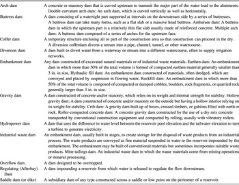
To formally assess the global imprint of dams on the environment requires firm numbers of dam size and distribution. An accurate global estimate of dams, however, is far from complete. The large range in the size of dams, differences in national accounting procedures and criteria, differences in ownership (public or private), and the extensive history of dams make arriving at a global tally of contemporary dams a challenging task. Additionally, there is no consensus on how to categorize dams. The British Dam Society identifies four types of dams while the U.S. Society on Dams identifies eleven types of dams (Table 4.2). Part of the issue is that dams are characterized in several ways, including their usage (purpose), construction materials, and design (shape).
While accounting of smaller dams will continue to be a work in progress, great improvements have been made in tallying larger dams so that a clearer global picture has emerged with regard to their distribution and characteristics. These data are essential to assess the broader environmental imprint of dams upon the landscape and water resources. Over the past decade or so, national and international stakeholder organizations have systematically accumulated information pertaining to a variety of dam criteria. Increasingly, these include important descriptive data such as dam height, type of dam, ownership, date of construction, purpose of dam, date of closure, reservoir capacity, river basin, upstream impounded area, streamflow volume, etc. The most authoritative and scholarly recognized organization for large dams is compiled by the International Commission on Large Dams (ICOLD), a nongovernmental organization (trade industry) that promotes standards and guidelines pertaining to best practices regarding construction and management of dams and reservoirs. ICOLD defines large dams as having a height of 15 m or greater (from foundation to dam crest) or a dam between 5 and 15 m that impounds greater than 3 million m3.
Data from the most recent ICOLD tally identifies 57,985 large dams (as of September 2019) across ninety-six member nations, providing a view as to their location and function (Figure 4.3A–C). China stands out as the global leader in large dams. About half (47%, 13,142) of the world’s large dams are constructed for the sole purpose of irrigation in support of agriculture, although an additional 6,180 large dams primarily built for irrigation have multiple purposes (flood control, hydropower, etc.). Large dams constructed for irrigation are especially concentrated in India, Spain, South Africa, Southeast Asia, and in the United States west of the hundredth meridian (Biemans et al., Reference Biemans, Haddeland and Kabat2011). Most significant large dam construction occurred over a four-decade period spanning the 1950s and 1980s, and earthen dam structures dominate (Figure 4.3). The total volume of reservoir impoundment exceeds 6,500 km3 (Figure 4.4), and will rapidly increase over the next several decades.
Global tally of large dams (57,985) from ninety-six member nations of the International Commission on Large DamsFootnote 1 (September 2019). Large dams are classified by (A) location (continent or region), (B) functions (sole function and multiple functions), and (C) types of large dams. Location (continent or region): China plotted separate from Asia because of very high number of large dams; Asia included Middle Eastern nations and Turkey because dams mainly in Tigris-Euphrates drainage to the Persian / Arabian Gulf; Australia and New Zealand classified together; North America included Canada, United States, and Mexico; Europe included Russia.


Global growth of reservoir storage capacity between 1900 and about 2010, including dams under construction and planned (U/C) between 2000 and 2010.

Advances in geospatial technologies such as high-resolution satellite imagery and topographic data (lidar) hold great promise for characterizing Earth’s impounded riparian landscapes (Walter and Merritts, Reference Walter and Merritts2008; Poeppl et al., Reference Poeppl, Keestra and Hein2015; Mulligan et al., Reference Mulligan, van Soesbergen and Sáenz2020). Such information can then be coupled with important landscape matrices, such as land cover, precipitation, streamflow volumes, slope, sediment loads, and other river basin indices. The Global Reservoir and Dam Database (GRanD), for example, assimilated a global geospatial database of dams mapped from 1800 to 2010 (Lehner et al., Reference Lehner, Reidy Liermann and Revenga2011). Although providing detailed attribute data on dams it includes only 6,862 records (<10% of global large dams). A recent effort at a global tally utilized several types of satellite imagery at varying spatial scales (i.e., Landsat, Ikonos, Spot imagery) to identify dams with concrete structures, including large dams from GRanD and ICOLD databases, in addition to some medium-sized dams. The GlObal geOreferenced Database of Dams (GOODD) contains >38,000 dams. Such approaches are also essential to identify long decommissioned dams – particularly numerous small dams – buried in historic (legacy) reservoir deposits, but which continue to influence contemporary fluvial riparian processes (i.e., Walter and Merritts, Reference Walter and Merritts2008; Poeppl et al., Reference Poeppl, Keestra and Hein2015; Brown et al., Reference Brown, Lespez and Sear2018).
If considering a larger range of impoundment types, including mill dams, low weirs, and primitive “check dams,” there are surely millions of dams on Earth. And if including impoundments with a minimum surface area of 100 m2, it is estimated there could be about 16 million dams on Earth. This potentially increases Earth’s freshwater surface area by 306,000 km2, a global increase of 7% (Lehner et al., Reference Lehner, Reidy Liermann and Revenga2011; Mulligan et al., Reference Mulligan, van Soesbergen and Sáenz2020).
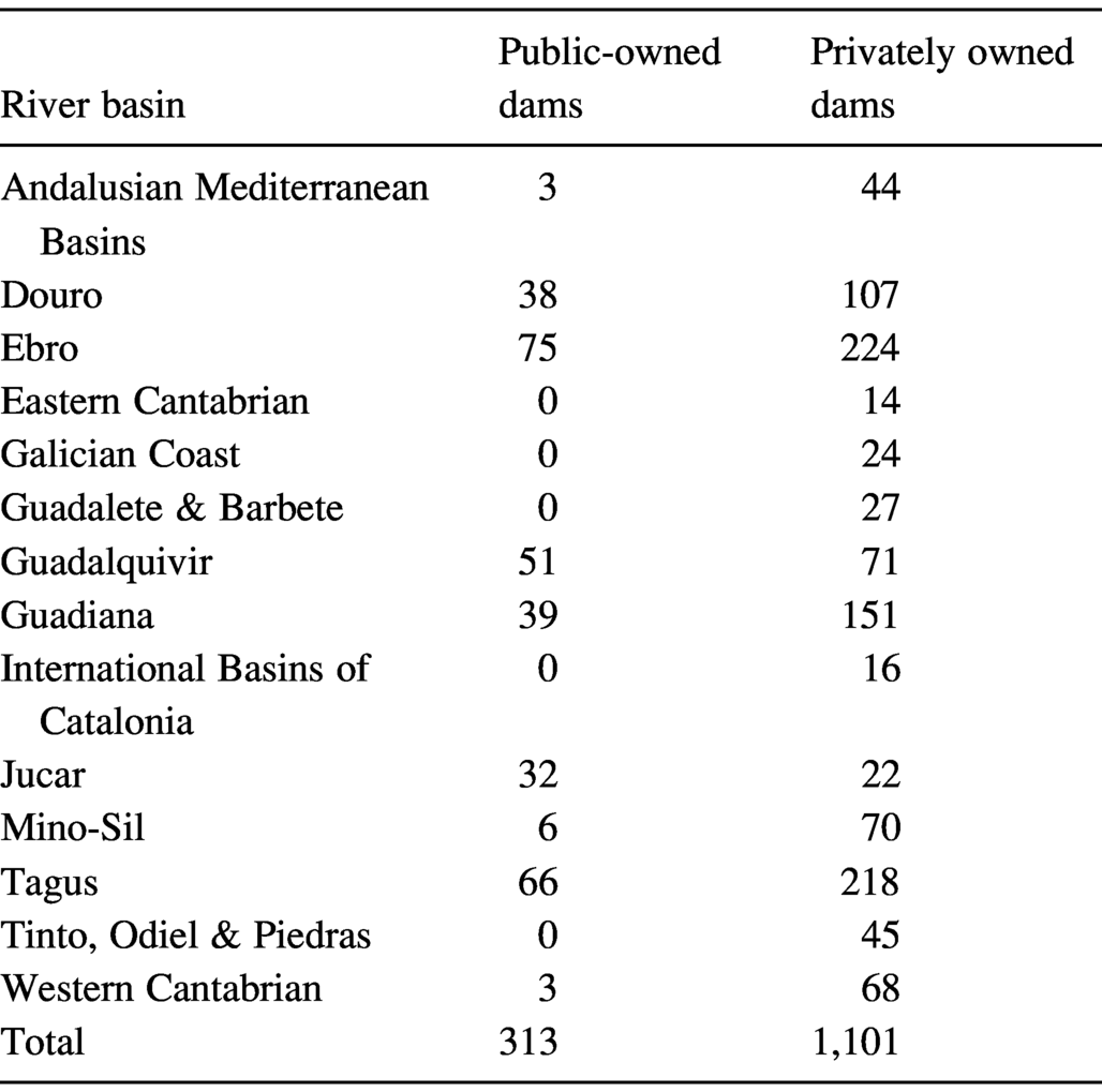
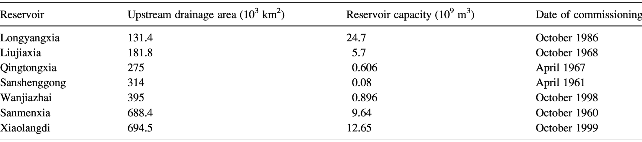
To further appreciate the scope of river disturbance by dams it is useful to provide data that pertain to specific basins and nations. In the United States, there are some 2.5 million dams impacting every basin larger than 2,000 km2 (NRC, 1992; Heinz Center, 2002; U.S. EPA, 2016). Most of China’s dam construction is in the Huanghe and Yangtze basins, with the latter having over 50,000 dams (Lehner et al., Reference Lehner, Reidy Liermann and Revenga2011; Yang et al., Reference Yang, Milliman, Li and Xu2011). India has 5,100 large dams (International Commission on Large Dams, www.icold-cigb.org/) and is heavily investing in dams and reservoirs, with 313 large dams under construction (NRDI, 2016). An important concern is that many of India’s dams under construction and proposed will be located in active seismic zones within the Himalayas, including regions that are intensely politically contested with Pakistan and China. Dams in India were historically overwhelmingly constructed for irrigation in support of agriculture and food security. India’s new mega dams, however, are being constructed primarily for hydropower. Indeed, India is now the world’s fifth largest hydropower producer (IWPDC, 2020). With 1,538 large dams (MITECO, 2020) Spain is the most impounded nation in Europe. This represents 2.5% of the world’s dams, and Spain’s dams have a total storage capacity of 54.6 km3 (Batalla, Reference Batalla2003). Although Spain also has Earth’s oldest functioning dam (Figure 4.5), most of Spain’s functional dams were constructed in the 1970s and 1980s and are privately owned (Table 4.3), with some 5,500 being less than 15 m in height (Figure 4.6).
World’s oldest dam. Roman era Cornalvo dam in Extremadura, Spain impounds the Rio Albarregas since 130 AD. The dam is part of a system of hydraulic infrastructure that supplies water to Emerita Augusta (Mérida) by aqueduct, similar to the adjacent.

Roman era Acueducto de los Milagros. The gravity dam has a concrete core and an outer earthen structure for support, with stone cladding. Size: 28 m high, 194 m long.

Height of large dams in Spain (total = 1,538).

Australia is the driest inhabited continent, and internationally has the highest per capita surface water impoundment of any nation (AWA). Australia has 557 large dams, according to the Australian National Committee on Large Dams (Figure 4.7). Most of Australia’s dams are in Queensland (120 dams), Victoria (113 dams), and New South Wales (135 dams), although much smaller and wet Tasmania has 100 large dams. Unfortunately, new large dams are proposed for tropical northern Australia, including the Fitzroy (Western Australia), Darwin (Northern Territory), and Mitchell (Queensland) basins. The main driver behind proposed dam construction is to provide water for irrigation to support massive investment in agricultural development.
Large dams in Australia organized by height (m). Large dams in Australia are >15 m, or >10 m if reservoir >1,000,000 m3 and maximum discharge >2,000 m3/s.

Canada has over 14,000 dams with 1,157 considered large dams (15 m high, or >5 m high and impounding >3,000,000 m3) and 49 dams considered very large (>60 m high) (Canadian Dam Association, 2019). Dam construction in Canada is overwhelmingly for hydropower, including 860 of its large dams. Dams constructed for irrigation are primarily in central and western provinces, including Saskatchewan, Alberta, Manitoba, and eastern portions of British Columbia. Most water demands for agriculture and industry are in the south, while Canada’s rivers mainly flow north. There are also many Canadian dams constructed to store mining tailings. Unlike in the United States, which has not constructed a large dam in decades, Canada has completed several large dam projects within the last decade and is finalizing works on a major dam to the Peace River in British Columbia.
The United States has a conflicted history with dams over about the past century, being a global leader in both dam construction and dam removal. The United States has 91,457 large dams (>1.8 m high) on its national registry (Figure 4.8), with 137 very large dams that each store more than 1.2 km3 of water (U.S. National Inventory of Dams, 2020Footnote 2). Of these dams, the average age is fifty-seven years, 7% are built for hydropower, 74% have a high hazard potential, and 69% are regulated at the state level (as of April 2020). Additionally, as with many nations, in the United States there are numerous small dams locally operated to manage small fishing ponds, farm ponds, amenity lakes, and old mill dams not in the NID. Many old mill dams, in particular, are obsolete and relict, having long lost their original purpose because of upstream land degradation and soil erosion driving reservoir infilling, particularly those constructed in the eighteenth and nineteenth centuries (Trimble, Reference Trimble1974; Walter and Merritts, Reference Walter and Merritts2008). As an example, for the Apalachicola-Chattahoochee-Flint basin (52,720 km2) in the US southeast, a GIS analyst identified over 25,000 reservoirs, although only 6% were included in the National Inventory of Dams (NID) database (Figure 4.8; U.S. EPA, 2016).
The United States has 91,457 dams.
Decade of completion.

Height.

Primary purpose.

Primary owner.

Primary type.

Hazard potential. Note: y-axis for dam type (E) is logarithmic.

4.2.2 River Fragmentation by Dams and Reservoirs
The environmental impacts caused by dams and reservoirs can be appreciated by considering changes to freshwater resources. From the standpoint of the volume of freshwater, in the beginning of the twentieth century, reservoirs increased global freshwater supplies over natural supplies by 5% (18 km3/yr). By the end of the twentieth century, the volume of surface water supplies had increased by 40% (460 km3/yr) over natural supplies (Biemans et al., Reference Biemans, Haddeland and Kabat2011). From the perspective of the global surficial footprint (area) of the impact of reservoirs, the cumulative area of irrigation increased from 40 Mha in 1900 to 215 Mha in 2000. Over half of Earth’s global runoff is regulated by dams, with most dams located in basins with heavy agriculture. The total cumulative storage capacity of reservoirs is ~20% of Earth’s annual runoff (Biemans et al., Reference Biemans, Haddeland and Kabat2011). The streamflow of all larger US rivers is impacted by dams, and a volume of water equal to 75% of the average annual runoff is stored in reservoirs (Graf, Reference Graf1999).
An important principle of impounded river management – and a cruel irony for riparian ecosystems and stakeholders – is that river basins in dry environments are more adversely impacted by dams than those in wet environments (Graf, Reference Graf1999; Magilligan et al., Reference Magilligan, Haynie and Nislow2008).
Dam construction is charging forward in Asia, South America, Africa, and the Balkans in Europe, despite vital environmental and management lessons learned from experiences across an international array of physical and economic settings. Of great concern is that an additional 3,700 large dams are either under construction or planned for construction. Incredibly, within about a decade the number of large hydroelectric dams on Earth will double (Figure 4.9). While this would provide an additional 1,700 GW of hydropower (Zarfl et al., Reference Grill, Lehner, Lumsdon, MacDonald, Zarfl and Liermann2015) it will come at a substantial environmental cost (e.g., Winemiller et al., Reference Winemiller, McIntyre and Castello2016; Zarfl et al., Reference Zarfl, Berlekamp and He2019). Should the planned dam construction be completed, a total of 89% of Earth’s flow volume would be impacted by dams, particularly in view of forthcoming impoundment of the Amazon (Grill et al., Reference Grill, Lehner, Lumsdon, MacDonald, Zarfl and Liermann2015).
Global acceleration of dam construction for hydropower per decade since 1900, including dams under construction and planned through the 2030s.

Unfortunately, the massive increase in dam construction is located within the headwater supply and transfer zones of some of Earth’s largest river basins, including the Yangtze and Amur Rivers in China. And new dams are especially being constructed within large tropical basins, such as the Amazon (368 new dams), Brahmaputra (396 new dams), Mekong (120 new dams), and Congo (35 new dams) Rivers (Zarfl et al., Reference Zarfl, Berlekamp and He2019). Damming tropical rivers is especially unfortunate because the riparian corridors representing among Earth’s highest biodiversity and the habitat of numerous riparian species – including charismatic aquatic megafauna as well as endemic and yet to be inventoried species – could be lost (Winemiller et al., Reference Winemiller, McIntyre and Castello2016; Latrubesse et al., Reference Latrubesse, Arima and Dunne2017).
The impacts of dams on drainage basin hydrology can be characterized by indices that quantify the degree of fragmentation (disruption to longitudinal connectivity) to the drainage network and also by the degree to which annual flow volumes are impounded (Graf, Reference Graf1999, Reference Graf2001, Reference Graf2006; Magilligan et al., Reference Phillips2003; Zarfl et al., 2014; Grill et al., Reference Grill, Lehner, Lumsdon, MacDonald, Zarfl and Liermann2015). Two approaches to assess the impact of dams on a river basin is the river fragmentation index (RFI) and the river regulation index (RRI). The RFI expresses the degree that riverine longitudinal connectivity is physically obstructed by dams (Figure 4.10), and strongly relates to the degree that fish migration is directly impacted by dams. The RRI expresses the degree that annual runoff of a basin is impounded by dams, and is important to issues related to downstream flow competence, water scarcity, and riparian habitat. Changes to the RRI and RII mirrored global dam construction over the twentieth century (Figure 4.10), and are expected to undergo sharp increases between 2010 and 2030 with the new boom in dam construction.
Global trend and future trajectory (to 2030) for the river fragmentation index (RFI) and river regulation index (RRI). Indices derived between 1930 and 2010 and estimated until 2030 (based on GRanD) for hydropower scenarios (dotted lines). Values reflect area-weighted means of indices across all basins.

While global changes to the RRI and RII over most of the twentieth century were somewhat similar, they often vary considerably for specific drainage basins because of differences in the types of dam constructed, and particularly because of basin hydroclimatology. The annual streamflow regime of the Danube, Europe’s second largest river, is minimally impacted by main-stem dams (RRI < 20%) because the reservoirs are essentially large narrow run-of-the-river structures that do not store much water relative to the large volume of annual runoff supplied from the humid headwaters. But the lower Danube is substantially fragmented by dams with an RFI of ~90%, which effectively means that fish migration no longer occurs. And Danube basin fragmentation is projected to become much worse if some 2,700–3,000 (small to large) hydropower dams in the Balkan headwaters are completed (Hockenos, Reference Hockenos2018; Zarfl et al., Reference Zarfl, Berlekamp and He2019).
A key concern as regards the Balkan dam boom is that they’re being hastily constructed with very little oversight, including very little baseline or post-dam environmental data. A total of 636 new hydropower dams are already operational in the Balkans. Alarmingly, a scant 2.2% of the dams had environmental monitoring stations within the upstream or downstream vicinity. This includes only fourteen of the dams with hydrologic monitoring stations, only six with fish monitoring stations, and only four had macroinvertebrate monitoring stations. The capability to conduct environmental impact assessments of the Balkan dam construction boom is severely hampered. And for Balkan nations in the EU it will be difficult to comply with the Water Framework Directive (Huđek et al., Reference Huđek, Žganecc and Puscha2020).
The RFI for the Amazon is expected to increase from near zero in 2010 to ~20% by 2030 because of the large number of dams being constructed (Grill et al., Reference Grill, Lehner, Lumsdon, MacDonald, Zarfl and Liermann2015; Latrubesse et al., Reference Latrubesse, Arima and Dunne2017). But because of the substantial annual runoff volumes of the Amazon, over the same period the RRI is only expected to increase from about zero to ~5% (Grill et al., Reference Grill, Lehner, Lumsdon, MacDonald, Zarfl and Liermann2015).
In contrast to humid regions, rivers impounded by reservoirs in semiarid settings tend to have higher RRI values, particularly with broad reservoirs in flat terrain. Rivers draining the US Great Plains and western interior regions, including the Colorado River basin, are the most heavily impacted in the United States because a large proportion of the basin’s total annual water yield is impounded within reservoirs (Graf, Reference Graf1999, Reference Graf2001). The high proportion of annual runoff impounded by dams produces considerable downstream water stress in dry regions, which is challenging when managing water for both irrigation and riparian ecosystems. While dry impounded regions in the United States are increasingly introducing dam and reservoir management strategies to mitigate the impact of altered streamflow regimes, in other dryland regions the rapid pace of dam construction is causing additional water stress.
4.2.2.1 Indus Basin Project
The Indus Basin Project is the world’s largest irrigation system and includes some 26.3 Mha of cultivated lands within a dry region fed by one of the world’s largest rivers. The irrigation project was born from the Indus Water Treaty signed in 1960, which has been a model of trans-boundary cooperation between India and Pakistan for seven decades. To manage water supply to the irrigation district three large reservoirs were constructed (Chashma, Mangla, and Tarbela). Additional hydraulic infrastructure comprising the irrigation project includes twelve inter-river canals, forty-five canals extending 60,800 km, twenty-three barrages and siphon structures, communal watercourses, farm channels, and field ditches that extend some 1.6 million km to provide water to over 90,000 farmer-organized water courses (FAO, 2016). The irrigated lands provide some 95% of Pakistan’s food production. But the system is fragile, needing repairs, and under stress because of increasing competition from hydropower dams in the Himalayan headwaters of the Indus basin (Raza et al., Reference Raza, Naeem and Qadeer2019).
Despite the long-term effectiveness of the Indus Water Treaty, the race to build mega dams in the Indus basin headwaters are straining relations between India and Pakistan, as well as China (Laghari et al., Reference Laghari, Vanham and Rauch2012; Raza et al., Reference Raza, Naeem and Qadeer2019). India is building several large hydropower plants in the Sutlej, Beas, and Ravi River basins that will impound streamflow that drains to Pakistan (FAO, 2016). China is building dams on the upper Sutlej River in China, which then drains to India before eventually joining the Indus River in Pakistan as a major tributary. Pakistan is constructing the Diamer-Bhasha Dam (2028 completion), which at 272 m high will be the tallest concrete filled roller dam in the world and have a massive storage capacity of 10 km3. Pakistan is also constructing the Bunji Dam (190 m high) on the upper Indus River main-stem as well as five additional dams to form a North Indus River cascade.
Collectively, the new Indus River basin dams will reduce water and sediment flow to the largest irrigation project in the world, particularly in Pakistan’s Punjab and Sindh provinces, the latter of which includes much of the heavily degraded Indus delta (Qureshi, Reference Qureshi2011; FAO, 2016). Already some 95% of Indus River water is extracted for irrigation before reaching the coast, with zero flow in prolonged dry periods (FAO, 2011). This means that the extensive irrigation districts in the dry lower basin and delta will experience additional water stress (Qureshi, Reference Qureshi2011), with expected declines in riparian and delta fisheries (Laghari et al., Reference Laghari, Vanham and Rauch2012).
Overall, new dam construction in the Indus Himalayan headwaters is projected to result in a modest increase in river fragmentation (RFI from ~60% to ~75% over 2010–2030), but because the structures are mega dams the degree of impoundment will be staggering, with the RRI increasing from ~30% to ~180% over 2010–2030 (Grill et al., Reference Grill, Lehner, Lumsdon, MacDonald, Zarfl and Liermann2015).
4.3 Environmental Impact of Dams and Reservoirs
4.3.1 Streamflow Regime
Upon impoundment, the impact of dams to streamflow is immediate and can be assessed by analyzing a time series of streamflow before and after dam installation (Figure 4.11). Changes to streamflow regime principally occurs in two ways: (i) a reduction in flow variability and (ii) a shift in seasonality of high- and low-flow periods (Graf, Reference Graf2001; Magilligan et al., Reference Magilligan, Haynie and Nislow2008). The former is manifest by a reduction in maximum (annual peak events) discharge and an increase in minimum (low) flows. The latter results in a change to the seasonality of high- and low-flow periods, potentially being out-of-phase with critical downstream ecological processes. The shift to a more monotonous flow regime is especially concerning because reduced flow variability directly reduces riverine geodiversity (i.e., physical integrity), to which riparian biodiversity is tightly dependent (Ward and Stanford, Reference Ward and Stanford1995; Nislow et al., Reference Nislow, Magilligan, Fassnacht, Bechtel and Ruesink2002; Pegg et al., Reference Pegg, Pierce and Roy2003; NRC, 2005). Channel morphologic features and geomorphic processes such as pools and riffles, sediment flushing, lateral migration, and planform geometry are controlled by moderate-sized discharge pulses at about bankfull or flood stage. Channel and floodplain (lateral) connectivity is crucial to providing riparian wetland ecosystems with nutrients and water, and for migration of aquatic organisms. Benthic riparian ecosystems require periodic “flushing flows” to cleanse algae from gravel, remove fine sediment from interstitial pores, reorganize meso-scale bed topography, and resupply spawning gravel (Power et al., Reference Power, Dietrich and Finlay1996). Because many dams are designed to provide water for crop cultivation, withdrawals for irrigated agriculture impose water stress on downstream riparian environments, particularly during vulnerable low-flow periods (Batalla et al., Reference Batalla, Kondolf and Gomez2004; van Dijk et al., 2013).
Conceptual model of annual flow regime for natural and impounded rivers, including “sawtooth” pattern from storage and release schedule for hydropower generation as well as withdrawal for irrigation to support agriculture during dry periods.

4.3.1.1 United States
The wide physical geographic variability across the United States elucidates regional differentiation on the downstream impacts of dams to streamflow regime. And the greatest impacts occur along rivers with a high ratio of reservoir storage capacity to mean annual water yield (~dry regions). At a national scale, very large dams in the United States have reduced annual peak discharge pulses by 67% and low-flow discharge has increased by 52%. The ratio between the annual maximum and mean flow has decreased by 60% (Graf, Reference Graf2006). These hydrologic changes are epitomized along the middle Missouri River, for example, where the post-impoundment discharge during the spring high-flow period is significantly lower, a critical issue because of coinciding during periods of fish spawning (Pegg et al., Reference Pegg, Pierce and Roy2003).
An additional important streamflow alteration with ecological implications is changes to the timing (seasonality) of high- and low-flow periods. This often occurs because of dam management in relation to stakeholder interests (e.g., irrigation schedules, electricity demands, recreation, flood management). In such cases, critical high-flow pulses may be offset by weeks to months. Rather than coinciding with the “natural” wet period, higher flows occur during low-flow periods (Graf, Reference Graf2006). The most problematic aspect of changes to the timing of high- and low-flow periods occurs when they are out of accord with the environmental rhythms of the riparian corridor, such as seed germination, avian water fowl nesting, or the dependence of fisheries lifecycles for feeding and spawning (Graf, Reference Graf2002; NRC, 2005; Górski et al., Reference Górski, van den Bosch and van de Wolfshaar2012), as discussed below.
The reduced streamflow variability of US rivers is mainly consistent with international trends in changes to downstream streamflow regime following impoundment and dam closure, with variation due to basin-specific physical and stakeholder influences, particularly in support of agriculture.
4.3.1.2 Europe: Ebro and Volga Rivers
Extensive national and regional analyses of the impacts of dams on flow regimes similar to that conducted in the United States (i.e., Graf, Reference Graf2006) have not been conducted for Europe. It is well acknowledged, however, that streamflow regimes of European rivers are heavily impacted by dams. Indeed, 90% of Earth’s most obstructed rivers are located in Europe (Kornei, Reference Kornei2020). An extensive analysis of pre- and post-dam streamflow trends for the Ebro basin (85,530 km2) in Spain identified reduced flow variability (Batalla et al., Reference Batalla, Kondolf and Gomez2004). This was manifest by higher low flows due to reservoir outflow during dry periods (summer) to support irrigation while the storage of winter streamflow reduced maximum flow values. The two-year and ten-year flood magnitudes were reduced by over 30% on average for most gauging stations, including in the lower Ebro River (at Tortosa) downstream of the Mequinenza and Ribarroja reservoirs (Figure 4.12).
Changes to flow regime for two large European rivers, before and after impoundment.
Reduction in annual maximum floods, lower Ebro River (at Tortosa) downstream of the Mequinenza and Ribarroja reservoirs.

Changes to lower Volga River discharge regime after dam closure over 1959–1960.

Like many large northern midlatitude rivers, the Volga (1,400,000 km2) serves as a major economic corridor. The Volga River is navigable for some 3,200 km through a series of eleven dams and canals that link northern ports along the White and Baltic to southern ports in the Caspian and Black Seas (Avakyan, Reference Avakyan1998; Middelkoop et al., Reference Middelkoop, Alabyan, Babich, Ivanov, Hudson and Middelkoop2015; Rodell et al., Reference Rodell, Famiglietti and Wiese2018). The Volga annually handles two-thirds of inland Russian navigation. Following impoundment of the lower Volga River behind the Volgograd Hydroelectric station in 1959 (at closure the largest hydroelectric dam in the world, remains largest in Europe), annual flow variability declined overall, including an increase in low flows by over ~1,000 m3/s (Figure 4.12B). The average maximum discharge reduced from 34,500 (m3/s) prior to dam closure (1959) to 26,800 (m3/s) after impoundment between 1959 and 1999 (Korotaev et al., Reference Korotaev, Ivanov and Sidorchuk2004). Of key importance to the hydrology of the lower Volga River is the vast amount of water withdrawn for industry, domestic use, and especially irrigation for agriculture, with the latter annually accounting for some 200 Mha of cultivated lands. Water consumption greatly increased following dam construction, increasing from 6 km3/yr pre-dam to 24 km3/yr post-dam, an amount that is about 10% of the water discharged into the Caspian Sea (Middelkoop et al., Reference Middelkoop, Alabyan, Babich, Ivanov, Hudson and Middelkoop2015). The Volga contributes 80% of the annual runoff supplied to the Caspian Sea, and annual water withdrawals for agriculture are contributing to Caspian Sea levels lowering (Rodell et al., Reference Rodell, Famiglietti and Wiese2018).
4.3.1.3 Yangtze and Three Gorges Dam
The streamflow regime downstream of the world’s largest dam, Three Gorges Dam (closure in 2003) along the middle Yangtze River has also changed downstream streamflow patterns (Zhang et al., Reference Zhang, Yuan, Han, Huang and Li2016; Tian et al., Reference Tian, Chang, Zhang, Wang, Wu and Jiang2019). Reduced flow variability extends some ~1,600 downstream, with reductions ranging from about 11% below the dam to 4% near the delta (Wang et al., Reference Wang, Shen, Gleason and Wada2013). These modest changes in river stage, however, mask hydrologic problems associated with management of Three Gorges Dam, in particular the abrupt up and down ramping and flow release schedule that produces frequent out-of-season flow variability. The flow release results in an oscillating pattern of drying out and backwater flooding of the massive floodplain lake system, including Poyang Lake (Zhang et al., Reference Zhang, Yuan, Han, Huang and Li2016). Not surprisingly, and with fair warning (i.e., Leopold, Reference Leopold1998), the downstream riparian environment has substantially degraded since closure of Three Gorges Dam, in association with sediment reduction and geomorphic adjustment (Zhang et al., Reference Zhang, Yuan, Han, Huang and Li2016; Cheng et al., Reference Cheng, Opperman, Tickner, Speed, Guo and Chen2018).
4.3.1.4 Nile, Aswan High Dam (Lake Nasser and Lake Nubia), and Water Politics
Because of its link to Egyptian antiquity, the historic Nile streamflow regime is perhaps the world’s most iconic coupled agro–hydro system, with irrigated agriculture extending along the entire Nile valley and across the delta plain (Figure 4.13). For over six millennia the Nile annually delivered nutrient-rich floodwater and silts to irrigated agricultural lands. But this abruptly ceased upon closure of the Aswan High Dam over 1965–1967 (Figure 4.14). The prior dynamic flow regime characterized by a seasonal fluctuation in river levels of 5–8 m has been greatly reduced to 1–2 m. As is common to downstream flow variability, Nile River low flows are moderately higher while the large annual flood pulses are greatly reduced, from ~8,000 m3/s to less than ~3,000 m3/s (Figure 4.15). A system of weirs downstream of Aswan High Dam maintains moderate flow stage levels to increase the river’s irrigation potential. Nile impoundment has greatly reduced annual runoff volumes, from 80 km3 to 30 km3 from pre-dam to post-dam, respectively (Liu et al., Reference Liu, Walling, Spreafico, Ramasmy, Thulstrop and Mishra2017). Although agricultural productivity increased with impoundment, the high demands on the irrigation system results in frequent water stress for some 95% of Egypt’s riparian population dependent upon the Nile River for 90% of its freshwater.
The Nile extends ~1,000 km from Aswan High Dam (bottom of image) to the delta without tributary inputs. Riparian agriculture effectively covers the entire valley and delta and contrasts with the hyper-arid Sahara.

Lake Nasser and Aswan High Dam, and Nile River in Egypt. Lake Nasser formed with dam closure over 1965–1967. The reservoir covers 5,250 km2 and extends for ~500 km, with 350 km as Lake Nasser in Egypt and 150 km as Lake Nubia in Sudan. Storage capacity for the reservoir is 162 billion m3. Reservoir sedimentation is measured regularly by bathymetric surveys along twenty-one fixed cross sections (Ahmed and Ismail, Reference Ahmed and Ismail2008). Scale: main axis of reservoir is ~3 km in width. North is to lower right of image.

Streamflow variability of Nile River below Aswan Dam between 1950 and 1985, revealing impacts to annual flood pulse (higher low flows, much lower peak flows) after dam closure over 1965–1967.

Today the main issue concerning Nile River management is located some 3,200 km upstream of Cairo and concerns impoundment of the Blue Nile by the Grand Ethiopian Renaissance Dam. As the largest reservoir in Africa, the Grand Ethiopian Renaissance Dam will store 1.5 times the average annual flow of the Blue Nile (Wheeler et al., Reference Wheeler, Basheer and Mekonnen2016). This will greatly increase the index of river impoundment (i.e., Grill et al., Reference Grill, Lehner, Lumsdon, MacDonald, Zarfl and Liermann2015) and, based on lessons learned from dam impacts on dryland rivers in the United States, the downstream riparian zone will be substantially degraded because of reduced flow variability (e.g., Graf, Reference Graf2006).
For well over a decade, imminent impoundment of the Blue Nile in Ethiopia has increased water stress and political tensions between Egypt and Ethiopia. Aside from the longer-term management scheme of the dam and reservoir – such as changes in water quantity, quality, and the outflow release schedule – a pressing issue receiving considerable international attention is the period of reservoir infilling (Wheeler et al., Reference Wheeler, Basheer and Mekonnen2016; El-Nashar and Elyamany, Reference El-Nashar and Elyamany2018). If the reservoir is rapidly infilled, it requires that the reservoir impounds all upstream Blue Nile waters (zero outflow). Even this extreme measure will require about three years to fill the reservoir to a level where hydropower turbines can be activated. And this is dependent upon the rainfall patterns over the Ethiopian highlands (El-Nashar and Elyamany, Reference El-Nashar and Elyamany2018). Such a rapid rate of reservoir infilling would effectively desiccate downstream riparian lands in Sudan, upstream of Egypt’s Aswan High Dam. International agreements between Nile basin nations with regard to water withdrawals have been especially ineffective but are particularly critical in view of imminent closure of the Grand Ethiopian Renaissance Dam (Wheeler et al., Reference Wheeler, Basheer and Mekonnen2016).
4.3.2 Impact of Dams to Fluvial Sediment Flux
4.3.2.1 Global Perspective
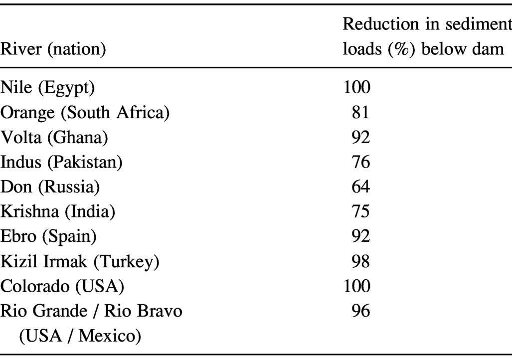
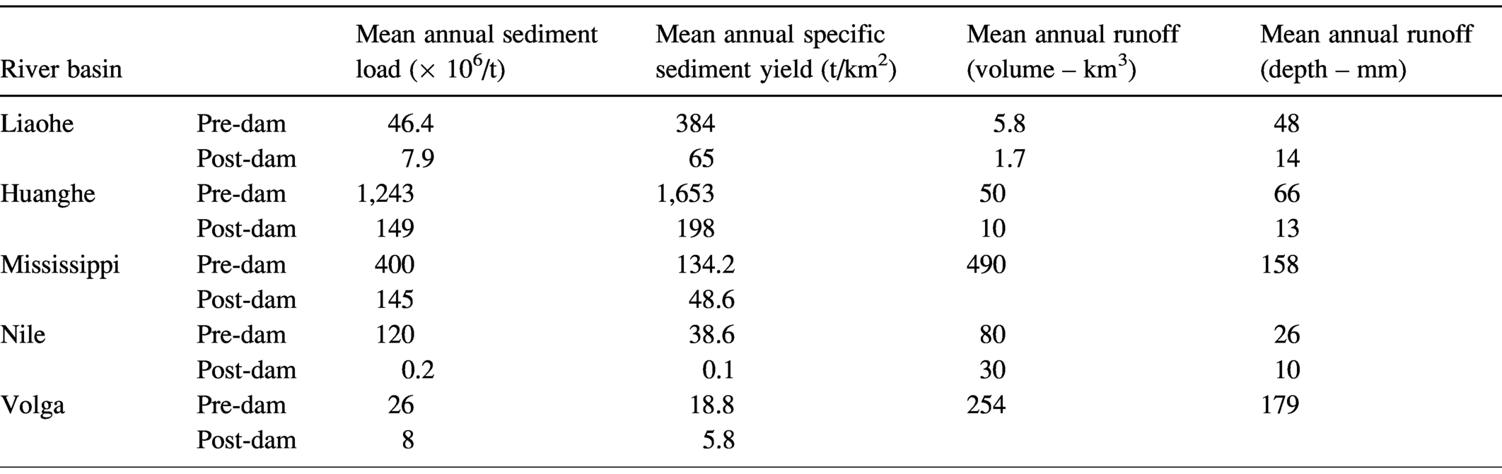
The global proliferation of dams means that copious amounts of Earth’s riverine sediments are trapped in upstream reservoirs, small and large (e.g., Morris and Fan, Reference Morris and Fan1998; Walling, Reference Walling2006; UNESCO-IHP, 2011; Tockner et al., Reference Tockner, Bernhardt, Koska, Zarfl and Hüttl2016). Trap efficiencies of main-stem dams along large rivers tend to be very high (Table 4.4), with many reservoirs trapping greater than 80% of upstream sediment flux (Vörösmarty et al., Reference Vörösmarty, Meybeck, Fekete, Sharma, Green and Syvitski2003). Many US dams, including large dams in the Mississippi basin, have trap efficiencies greater than 95%. The large main-stem Colorado dams trap up to 100% of upstream sediment loads (except when intentionally flushed), as does the Nile River upstream of the Aswan High Dam (Williams and Wolman, Reference Williams and Wolman1984).
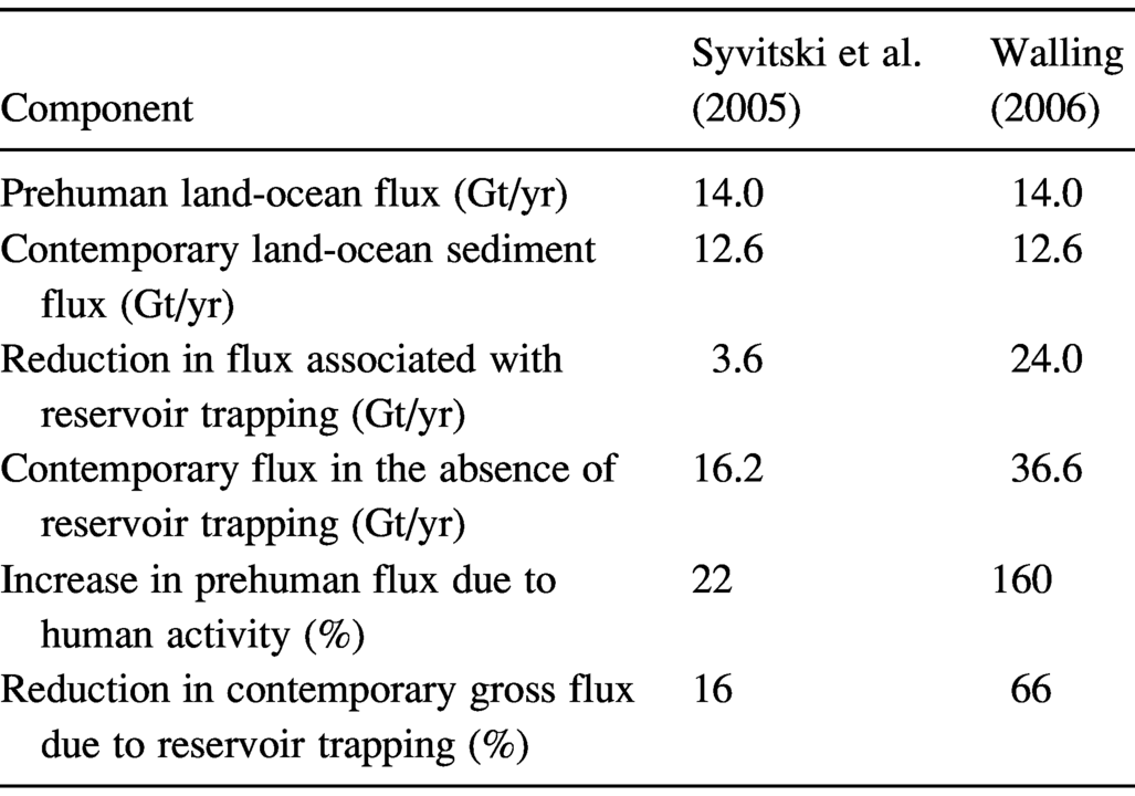
Fluvial sediment delivery to the coast has precipitously declined since the mid-1900s (Syvitski et al., Reference Syvitski, Vörösmarty, Kettner and Green2005; Walling, Reference Walling2006; UNESCO-IHP, 2011). Globally, some 12.6 GT of sediment loads are annually discharged into the oceans (Table 4.5). While estimates vary widely, the global decline in sediment flux ranges from 16% to 66% of annual riverine sediment loads (Syvitski et al., Reference Syvitski, Vörösmarty, Kettner and Green2005; Walling, Reference Walling2006). Much of the decline in sediment flux is attributed to the impact of dams, although improved land management, channel engineering, and climate change also reduces sediment loads (Batalla et al., Reference Batalla, Vericat and Martínez2006; Wang et al., Reference Wang, Yang, Saito, Liu and Xiaoxia2007; Walling, Reference Walling2008b; Meade and Moody, Reference Meade and Moody2010; Liu et al., Reference Liu, Walling, Spreafico, Ramasmy, Thulstrop and Mishra2017). Because dam construction coincides with different periods of human activities and climatic fluctuation, changes to sediment loads after dam closure can vary greatly from river basin to river basin (Table 4.6).
Reservoir sediment storage has diverse implications to fluvial environments. This includes upstream, within, and downstream of the reservoir (Table 4.7). Reservoir sedimentation can result in upstream flooding and reduced navigation, and aquatic habitat degradation. Problems associated with sediment storage in reservoirs includes reduced hydropower potential because of reduced storage capacity, storage of contaminated sediments, and reservoir stratification impacting aquatic habitat within the reservoir and downstream (discussed further, below). The high sediment trap efficiency of many dams substantially reduces downstream fluvial sediment loads, with consequences to geomorphic adjustments and riparian habitat. In addition to the quantity of sediment being reduced, the quality of sediment is often also reduced. In combination with the altered flow regime fine bed material is removed, resulting in downstream channel bed material becoming coarser, and in some cases leading to channel bed armoring.

4.3.2.2 Sediment Decline to Nile, Link to Agriculture
For millennia, rains in the Ethiopian Highlands generated runoff that transported some 95% of the Nile River’s sediment load. Sediment was principally supplied to the main-stem Nile by the Blue Nile (324,530 km2) and Atbara (166,875 km2) Rivers, both of which enter the main-stem Nile upstream of Aswan High Dam. But after impoundment behind the Aswan High Dam all upstream Nile sediment is stored in Lake Nasser (Ahmed and Ismail, Reference Ahmed and Ismail2008; Liu et al., Reference Liu, Walling, Spreafico, Ramasmy, Thulstrop and Mishra2017). Suspended silt concentrations averaged 3,800 mg/L between 1929 and 1963 but abruptly declined to only 129 mg/L by 1965, two years after the start of infilling Lake Nassar reservoir (Raslan and Salama, Reference Bakkenist and Flos2015). The average annual sediment load in the pre-dam period was 120 million tons, but was reduced to 0.2 million tons after dam construction (Liu et al., Reference Liu, Walling, Spreafico, Ramasmy, Thulstrop and Mishra2017). Further downstream, sediment loads in the Nile only marginally recover, as there are no appreciable tributaries for about the final 1,000 km (Figure 4.16). A minor amount of sediment is supplied from aeolian inputs, bank erosion and channel bed scour. Low flow structures (weirs) control stage levels in support of navigation and floodplain irrigation (Morris and Fan, Reference Morris and Fan1998; Ahmed and Ismail, Reference Ahmed and Ismail2008). At the coast the Nile discharges very little sediment (~5 × 10⁶ tons/yr) to the Mediterranean, with the substantial reduction in sediment loads contributing to coastal erosion and retreat of the Nile Delta (Stanley and Warne, Reference Stanley and Warne1998).
Downstream changes to suspended sediment loads along the Nile River before and after closure of Aswan High Dam in 1964. Suspended sediment comprises 30% clay, 40% silt, and 30% fine sand (Ahmed and Ismail, Reference Ahmed and Ismail2008).

Impacts to the Nile sediment and streamflow regime caused by the Aswan High Dam aren’t merely significant, they’re symbolic. The lower Nile is the premier example of a millennia-old, intensive floodplain-agricultural coupled system, especially dependent upon annual floodwaters and sediment for irrigation and fertility. As an early hearth of irrigation science, Nile farmers utilized an ingenious system of sluice gates, water wheels, dams, and buckets to maximize the potential of furrow-and-field irrigation methods (Butzer, Reference Butzer1976). But the iconic floodwater irrigation system was all but eliminated with construction of the Aswan High Dam, and initially reduced downstream productivity. Crop yields have increased since the dam was completed, but at a high cost. The Nile delta has continued to degrade because of a lack of fluvial sediment (Becker and Sultan, Reference Becker and Sultan2009; Stanley and Clemente, Reference Stanley and Clemente2014), and Nile delta agriculture now requires significantly larger “hard engineering” structures, including larger canals, ditches, and larger mechanical pumps for irrigation and drainage (Molle, Reference Molle2018). Additionally, the Nile agricultural system is dependent upon high amounts of chemical fertilizer to maintain high agricultural yields, an issue that results in interesting and unintended impacts to coastal fisheries production (Nixon, Reference Nixon2003), as noted further in text. Of course, the artificially high water table is problematic with regard to the annual deficit in rainfall (165 mm/yr) relative to evapotranspiration (1,500 mm/yr), and results in land degradation through soil salinization (Ahmed and Ismail, Reference Ahmed and Ismail2008; Molle, Reference Molle2018).
4.3.2.3 Sediment Decline to Yangtze and Huanghe Rivers
Some of the large rivers in Asia have more recently experienced sharp reductions in sediment loads following dam construction, and the changes continue to rapidly unfold because of many new dam construction projects (Syvitski et al., Reference Syvitski, Vörösmarty, Kettner and Green2005; van Binh et al., Reference van Binh, Kantoush and Sumi2019). This is particularly true of the Yangtze and Huanghe Rivers in China. Suspended sediment loads along the Yangtze River downstream of Three Gorges Dam at the lowermost sediment station (Datong, 565 km upstream of the delta) were already in decline. In the 1950s and 1960s, suspended sediment load averaged 507 Mt/yr but had declined in the period before dam construction to 320 Mt/yr (1993–2003). After closure of Three Gorges Dam (TGD), the sediment loads between 2003 and 2012 steeply dropped (Figure 4.17), to 145 Mt/yr. Between 2003 and 2012, an astonishing 182 Mt/yr (80% of the total sediment load) was trapped behind Three Gorges Dam (Yang, et al., Reference Yang, Xu, Milliman, Yang and Wu2015). Between 2002 and 2008, the median particle size (d50) of the channel bed material increased from 0.36 mm to 25 mm at Yichang (44 km downstream of TGD) but only increased from 0.18 mm to 0.19 mm at Chenglinji (420 km downstream of TGD) (Zheng et al., Reference Zheng, Xu, Cheng, Wang, Xu and Wu2018). Between these two stations (at 195 km downstream of TGD), the d50 of bed material increased from 0.19 mm (pre–TGD) to 0.251 mm by 2010, seven years after closure (Zhang et al., Reference Zhang, Yuan, Han, Huang and Li2016).
Comparison of annual discharge and suspended sediment loads before and after impoundment of the Yangtze River by Three Gorges Dam: Pre-dam (1993–2002) and post-dam (2003–2012). Datong is 565 km upstream of the river mouth.

The Huanghe River is also referred to as the Yellow River because of its ochre colored sediment that derives from erosion of the Chinese Loess Plateau. The Huanghe previously transported 1.08 Gt of sediment per year to the coast (at Lijin, 40 km from delta) – Earth’s highest annual sediment load. By 2005 this had declined to 0.15 Gt/yr, which is only 14% of its historic sediment load (Wang et al., Reference Wang, Yang, Saito, Liu and Xiaoxia2007).
A key reason for the decline in sediment loads of the Huanghe River is construction of seven main-stem dams between 1968 and 1998 (Table 4.8). It should be noted, however, that in addition to main-stem dam emplacement several other explanations are also responsible for the large decline in sediment loads over the past several decades, for both the Huanghe and Yangtze Rivers. These include improved land management (noted in Chapter 2), increased water withdrawals for agriculture and industry, and reduced precipitation due to climate change (Walling, Reference Walling2006; Wang et al., Reference Wang, Yang, Saito, Liu and Xiaoxia2007; Yang et al., Reference Yang, Xu, Milliman, Yang and Wu2015; Shi et al., Reference Shi, Hu, Deng, Tian, Wieprecht, Haun, Weber, Noack and Terheidenet2017). For the Huanghe, the impact of main-stem dam construction and improved management of the Loess Plateau has been so effective at reducing downstream sediment loads that downstream channel engineering measures were implemented to manage channel bed incision. Between the 1960s and 2000, soil conservation in the Chinese Loess Plateau reduced sediment inputs into the Huanghe River by some ~300 × 106 tons/yr. On the Yangtze, 65% of the reduction in downstream sediment loads since 2003 is attributed to closure of Three Gorges Dam, 5–14% is attributed to climate change (reduced precipitation), and the remaining cause of sediment load reduction is attributed to upstream dams and soil conservation (Chen et al., Reference Chen, Wei, Fu and Lu2007; Yang et al., Reference Yang, Xu, Milliman, Yang and Wu2015).
4.3.2.4 Sediment Decline Following Mekong Dam Construction
The Mekong delta receives much less sediment than before construction of a cascade of dams along the upper Mekong (Lancang) in China, which started with closure of Manwan Dam in 1993. The most recent analysis of “before and after” comparison of sediment loads shows a large sediment flux reduction to the Mekong delta, by some 74%. The pre-dam (before 1993) sediment flux to the Mekong delta was 166.7 million tons/yr (±33.3) but has now declined to 43.1 million tons/yr for 2012–2015 (van Binh et al., Reference van Binh, Kantoush and Sumi2019), which varies by ±20 million tons per year depending on whether ENSO is in a negative or positive phase, respectively (Ha et al., Reference Ha, Ouillon and van Vinh2018).
Closure of the Manwan Dam on the upper Mekong main-stem abruptly reduced downstream suspended sediment loads by >60% at Gajiu, 2 km below the dam, with modest sediment recovery further downstream (Fu et al., Reference Fu, He and Lu2008). Between 1993 and 2003, 26.9–28.5 million tons/yr were trapped in the Manwan reservoir, resulting in reservoir sediment storage of 295.9–313.5 million tons over an eleven-year period (Fu et al., Reference Fu, He and Lu2008). The large amount of reservoir sedimentation is concerning, as 21.5–22.8% of the total storage capacity of the Manwan reservoir was lost over an eleven-year period following impoundment. As a whole, the trap efficiency of six large main-stem dams along the upper Mekong in China ranges from 61% to 92% (Figure 4.18). As regards downstream sediment loss this is alarming when considering that some thirteen additional main-stem dams are planned or under construction upstream, toward the basin headwaters (Kummu and Varis, Reference Kummu and Varis2007; Fan et al., Reference Fan, Hea and Wang2015) (Figure 4.19). And already thirty-seven more dams exist in the lower basin in Laos, Cambodia, Thailand, and Vietnam.
The “stair-step” profile of a ~1,000 km segment of the upper Mekong (Lancang) River in China, upstream of Laos border, including trap efficiency (%), hydraulic head, dam height, and year of closure. *Upstream of this reach, seven large main-stem dams are under construction, including Miaowei (140 m high), Dahuaqiao (106 m), Huangdeng (202 m), Tuoba (158 m), Lidi (74 m), Wunonglong (136.5 m), and Gushui (220 m); and further upstream, six additional main-stem hydroelectric dams are planned or in construction, extending the stair-step profile toward the Himalayan headwaters.

Location of large dams (> 15-m height) in the Mekong basin, including completed, under construction, and planned. The border between the Upper Mekong (Lancang) and Lower Mekong divide is indicated. The “3S” river basins refer to the Sekong, Sesan, and Srepok Rivers, which join to form the largest tributary in the lower Mekong.

Detecting changes to the Mekong delta sediment flux highlights the importance of having continuous sediment records before and after impoundment, having sediment gauging stations in key upstream and downstream locations within the drainage basin, and having access to the data (Walling, Reference Walling2008a, Reference Walling and Campbell2009). A study by van Binh et al. (Reference van Binh, Kantoush and Sumi2019) provides the longest period of analysis – spanning five decades – that envelops the pre- and post-dam periods (1961–2015). Crucially, the analysis utilizes sediment load data for years 1965–2003 at the Jiuzhou station (China), above the upper Mekong cascade of dams.
The post-dam period for the Mekong River is a story that continues to unfold because of construction and planning of numerous large dams (Figure 4.19) throughout the basin (Walling, Reference Walling2008a,Reference Wallingb; Pokhrel et al., Reference Pokhrel, Burbano, Roush, Kang, Sridhar and Hyndman2018). Because of the large amount of drainage area in the lower Mekong, there is concern over the ongoing and future development of forty-two dams in the Se San, Srepok, and Se Kon Rivers in the lower basin, which join together to form the largest tributary to the Mekong. If the 133 dams planned for the Mekong are constructed only 4% of the Mekong River sediment load will be discharged to the delta (Kondolf et al., Reference Kondolf, Gao and Annandale2014a, Reference Kondolf, Rubin and Minear2014b; van Binh et al., Reference van Binh, Kantoush and Sumi2019), which would be devastating to the deltaic geomorphology and associated aquatic environments (Piman and Manish, Reference Piman and Manish2017).
4.3.2.5 Sediment Decline for Several European Rivers: Rhine, Ebro, Volga
The sediment loads of European rivers have been impacted by humans for centuries and millennia. Several rivers are representative of the impacts of dams to European rivers, including the Ebro, Volga, and Rhine Rivers.
A longitudinal profile of the Rhine River basin reveals the artificial stair-step pattern in the Upper and High Rhine because of intensive impoundment. This includes the Iffezheim Dam, the lowermost and last dam to be emplaced along the main-stem Rhine River (Figure 4.20). Suspended sediment loads along the Rhine River (185,000 km2) has increased and decreased with episodes of land cover change and hydraulic engineering (Vollmer and Goelz, Reference Vollmer and Goelz2006; Spreafico and Lehmann, Reference Spreafico and Lehmann2009; Middelkoop et al., Reference Middelkoop, Erkens and van der Perk2010; van der Perk, Reference van der Perk, Sutaria, Middelkoop, Stouthamer, Middelkoop, Kleinhans, van der Perk and Straatsma2019). The more recent episode, since about the 1950s, reveals about a 70% decline, which is dramatic for a river that had already been intensively impacted by human activities. Annual suspended sediment loads declined from 4 × 10⁶ tons to 1.2 × 10⁶ tons by 2016, and have remained relatively stable over about the past ten years (van der Perk, Reference van der Perk, Sutaria, Middelkoop, Stouthamer, Middelkoop, Kleinhans, van der Perk and Straatsma2019). The primary source of the decline since the early 1950s is likely the completion of two main-stem dams in the Upper Rhine, specifically Gambsheim and Iffezheim dams (Figure 4.20) completed in 1974 and 1977, respectively. As a whole there are twenty-one main-stem dams on the Upper and High Rhine. The sediment starvation problem along the Rhine has resulted in channel bed incision along large reaches of the main-stem Rhine in the delta and alluvial valley (Quick et al., Reference Quick, König, Baulig, Schriever and Vollmer2020) that threatens navigation and associated infrastructure, requiring innovative sediment management approaches (see Section 8.2.3).
Longitudinal profile of the Rhine River, including geomorphic province, major tributaries, and sediment management operations. The stair-step pattern in the Upper and High Rhine is due to intensive impoundment. Gambsheim hydroelectric dam is located at 309-km, 25 km upstream of Iffezheim dam.

The sediment flux of the lower Ebro River (85,530 km2) was historically high, annually discharging 20–30 million tons/yr into the Mediterranean (late nineteenth century). But the Ebro suspended sediment loads abruptly declined to 3.3 million tons/yr following a period of dam building in the early 1960s. By the early 2000s, and ~299 dams later, the sediment load transported to the delta had declined to a meager 0.29 million tons/yr – less than 2% of pre-dam sediment loads (Rovira and Ibàñez, Reference Rovira and Ibàñez2007). The dramatic reduction in Ebro River sediment load has had substantial adverse consequences to its delta, and ground subsidence is of particular concern (Tena and Batalla, Reference Tena and Batalla2013). About 45% of the emergent Ebro delta will be drowned by 2100 because of subsidence and rising sea levels. The strategy to mitigate against higher sea levels includes building new lands by sediment diversion structures within the delta and managing reservoir sediment by flushing operations to mobilize stored reservoir deposits for transport through a cascade of reservoirs (Rovira and Ibàñez, Reference Rovira and Ibàñez2007; Tena and Batalla, Reference Tena and Batalla2013).
Impoundment of the lower Volga River behind the Volgograd Dam trapped sediments and resulted in a large decline in annual suspended sediment loads. Prior to dam closure (1934–1953), the suspended sediment loads of the lower Volga River were 12–18.5 million tons/yr, which declined to 7.4 million tons/yr in the post-dam period (1961–1982). The annual suspended sediment load at the delta apex substantially declined from the pre-dam to the post-dam period, being 26 million tons/yr and 7.9 million tons/yr, respectively (Middelkoop et al., Reference Middelkoop, Alabyan, Babich, Ivanov, Hudson and Middelkoop2015).
4.3.2.6 Sediment Decline to Missouri and Mississippi Rivers
The fact that upstream dam efficiencies are so high and that a lot of fluvial sediment still makes it to the coast implies that sediment loads somewhat recover (Williams and Wolman, Reference Williams and Wolman1984; Phillips et al., Reference Phillips, Slattery and Musselman2004). This occurs largely because of downstream channel scour and erosion (discussed subsequently) and because impacts of upstream dam trapping can be buffered by sedimentary inputs from downstream tributaries. The downstream sediment load recovery is often less than 50% of upstream sediment loads.
Following closure of the downstream-most main-stem dam in 1955 on the Missouri River, Gavins Point Dam in North Dakota and South Dakota (Figure 4.21), downstream suspended sediment loads immediately declined by 99%. At Hermann, Missouri, a distance of 1,047 km downstream of Gavins Point Dam, suspended sediment loads in the post-dam period (1957–1980) only recovered to ~30% of pre-dam amounts (Figure 4.22), which includes sediment inputs from the Platte River basin (10.1 × 10⁶ tons/yr) (Heimann, Reference Heimann2016). The precipitous decline in suspended sediment loads is detected further downstream in the middle Mississippi River (at St. Louis, Missouri), and all the way downstream to the Mississippi delta (Figure 4.23).
Gavins Point Dam and Lewis and Clarke Lake, the lowermost dam on the Missouri River. The structure is an embankment dam of earthen and chalk-fill materials. Dimensions: closure in 1955, upstream drainage: 723,825 km2, 23 m high, 2,650 m long, total reservoir capacity is 606,873 m3, surface area of 12,700 ha, depth of 14 m, and maximum length of 40 km.

Historic changes to suspended sediment loads along the Missouri and Mississippi Rivers in relation to impoundment by large main-stem dams.

Ratio of pre-dam and post-dam suspended sediment loads along the Missouri River downstream from Gavins Point Dam (closure in 1955) in South Dakota to below the confluence with the Mississippi River at St. Louis, Missouri. Stations and pre- and post-year dataset include Yankton (1940–1952, 1957–1969), Omaha (1940–1952, 1957–1973), St. Joseph, Kansas City, and Hermann (1949–1952, 1957–1976) located 8, 314, 584, 716, 1,147 km downstream from Gavins Point dam.

As the case with many larger rivers, the timing of dam construction in the Mississippi basin occurred while other forms of hydraulic engineering and land cover change were also occurring, which further reduced downstream suspended sediment loads (Figure 4.24). Additional factors that reduced downstream suspended sediment loads in the Mississippi include improved land management in the upper basin (as with the Huanghe and Yangtze Rivers) and channel engineering in the lower basin. As channel bank erosion was previously a source of sediment for the lower Mississippi River, hydraulic engineering works such as groyens (wing dikes) and concrete revetment further reduce downstream sediment loads (Kesel et al., Reference Kesel, Yodis and McCraw1992; Kesel, Reference Kesel2003; Meade and Moody, Reference Meade and Moody2010).
Historic change to suspended sediment loads for the lower Mississippi River at Tarbert Landing, Louisiana. Trend lines coincide with years 1950–1967 (−15 million tons/yr) and 1968–2006 (−1.1 million tons/yr). Cumulative distance (km) for revetment and wing dike (groyne) construction included for USACE Memphis and Vicksburg Districts.

4.3.3 Impacts to River Channels
It is difficult to conceive of anything that could more fundamentally disturb an alluvial river than a large dam obstructing streamflow and trapping the vast majority of its sediment. And considering the sophistication of the science it is somewhat surprising that in 2021 we’re unable to accurately predict the direction, style, magnitude, spatial extent, and duration over which downstream geomorphic adjustment to a river will occur upon impoundment – at a level of precision useful to direct management decisions. More than anything, this serves as a reminder as regards the complexity and uniqueness of each fluvial system, and that subtle – but significant - differences in slope, particle size, flood regime, etc. result in varying forms of fluvial adjustment to flow impoundment (Williams and Wolman, Reference Williams and Wolman1984; Brandt, Reference Brandt2000; Phillips, Reference Phillips2003). And as much as any subject that concerns lowland rivers, the inability to precisely and accurately predict downstream fluvial adjustment to dams highlights the importance of a local – case-by-case approach – that requires copious field and ground data.
A fundamental change that occurs to initiate channel bed incision is the “hungry water” phenomenon. This develops because sediment loss due to upstream reservoir trapping results in excess stream power and sediment transport capacity downstream relative to the sediment load available for transport (Kondolf, Reference Kondolf1997; Habersack et al., Reference Habersack, Jäger and Hauer2013). Provided the channel bed is close to the threshold of erosion (i.e., Figure 2.22), the excess stream power is then able to incise the channel bed (Williams and Wolman, Reference Williams and Wolman1984; Wilcock, Reference Wilcock1998; Chin et al., Reference Chin, Harris, Trice and Given2002; Smith et al., Reference Smith, Morozova, Pérez-Arlucea and Gibling2016). Channel bed incision can then destabilize channel banks and lead to lateral widening, resulting in increased channel width (i.e., Figure 2.24). In the case of bedrock controls, channel incision may be limited, although lateral migration and increased channel widening may be substantial.
The benchmark works by Williams and Wolman (Reference Williams and Wolman1984) and Graf (Reference Graf1999, Reference Graf2006) analyzed large databases spanning considerable geomorphic and climatic variability, and provide signposts to make several general statements about the downstream impacts of dams to rivers because of altered streamflow patterns and “hungry water.” Following impoundment, rivers are likely to undergo incision, especially immediately downstream of the dam, with some lateral adjustment, especially if the channel banks are noncohesive and if the streamflow regime is not significantly altered. The magnitude of incision diminishes with distance downstream. Reduced flow variability results in channel narrowing, and a formerly active floodplain is likely to become stabilized by encroaching woody vegetation to the detriment of aquatic and riparian habitat (Marston et al., Reference Marston, Mills, Wrazien, Bassett and Splinter2005). Most of the main-stem channel adjustment occurs within about the first decade, and continues for decades although it is difficult to generalize how much, and for how far downstream the geomorphic adjustment will occur.
Temporally, the pattern of channel bed incision for rivers spanning a range of geologic and climatic settings mainly follows a negative exponential pattern. A number of channel cross sections along the Missouri, Colorado, Red, and Chattahoochee Rivers in the United States reveal channel bed incision ranging from about 0.5 m to 6.0 m (Figure 4.25). Most of the channel bed incision occurs within about the first decade, and then decreases or ceases over subsequent decades. The temporal pattern of adjustment may also be somewhat linear or stepwise, and Williams and Wolman (Reference Williams and Wolman1984) were careful to emphasize both “regular” and “irregular” styles of channel bed degradation, including incision and channel widening by lateral adjustment, following flow impoundment.
Channel bed adjustment for several US rivers, with river and station names relative to distance downstream of dams (on figure).

Europe’s two largest rivers exhibit clear downstream channel bed incision following impoundment (Figure 4.26). The lower Volga River underwent some ~1.5 m of incision following impoundment behind Volgograd Dam in 1960, and continued to incise (Figure 4.26A). A consequence of channel bed incision is that floodplain connectivity occurs by less frequent higher-discharge magnitudes (Middelkoop et al., Reference Middelkoop, Alabyan, Babich, Ivanov, Hudson and Middelkoop2015).
Channel bed incision for Europe’s two largest rivers revealed with hydrologic data.
Lower Volga River at Volgograd, Russia inferred by changes to stage-discharge relationships. Channel bed incision likely prior to 1969 data (dam closure over 1959–1960).

Incision of upper Danube River in Austria inferred with low water level data between 1950 and 2003 (at Wildungsmauer) following intensive impoundment from the 1950s to 1990s.

Following extensive upstream impoundment in the 1950s the Danube River in Austria, for example, illustrated a pattern of adjustment that is somewhat opposite many US rivers (Figure 4.26B). The Danube basin is intensively fragmented by dams (Grill et al., Reference Grill, Lehner, Lumsdon, MacDonald, Zarfl and Liermann2015). Sixty-nine dams were constructed in the upper Danube basin between the 1950s and 1990s that resulted in some 90% of the upper Danube being impounded (Habersack et al., Reference Habersack, Hein and Stanica2016). Effectively, no coarse sediment makes it over the main-stem dams along the Danube. Despite some 200,000 tons of coarse sediment annually being dumped downstream of the Freudenau hydropower dam in Vienna, higher shear stress downstream of the dam results in channel bed incision (Habersack et al., Reference Habersack, Jäger and Hauer2013). The annual rates of channel bed incision average ~2.0 cm/yr, and channel bed lowering continues (Habersack et al., Reference Habersack, Hein and Stanica2016). An additional influence on channel bed incision of the Danube is that, as with many rivers intensively utilized for navigation and settlement in Europe and North America (Hudson and Middelkoop, Reference Hudson, Middelkoop, Hudson and Middelkoop2015; Quick et al., Reference Quick, König, Baulig, Schriever and Vollmer2020), channel straightening and other hydraulic engineering works have reduced lateral sediment inputs and altered flow patterns, further driving channel bed incision (Habersack et al., Reference Habersack, Hein and Stanica2016; Schmutz and Moog, Reference Brown, Lespez and Sear2018).
4.3.3.1 Downstream Propagation of Channel Degradation
Spatially, along large rivers, channel bed degradation following impoundment may extend for tens to hundreds of kilometers downstream of the dam (Ma et al., Reference Ma, Huang, Nanson, Li and Yao2012; Smith et al., Reference Smith, Morozova, Pérez-Arlucea and Gibling2016; Smith and Mohrig, Reference Smith and Mohrig2017; Quick et al., Reference Quick, König, Baulig, Schriever and Vollmer2020). The amount of incision usually declines with downstream distance, being dependent upon the amount of change to the sediment and streamflow regime, the location and character of downstream tributary inputs, as well as the sedimentology and lithology of channel bed and bank material, valley slope, and human impacts (Brandt, Reference Brandt2000; Chin et al., Reference Chin, Harris, Trice and Given2002; Phillips et al., Reference Phillips, Slattery and Musselman2004; Smith et al., Reference Smith, Morozova, Pérez-Arlucea and Gibling2016; Lai et al., Reference Lai, Yin and Finlayson2017).
The closure of Three Gorges Dam in 2003 was a watershed moment in environmental sciences. Because of being the world’s largest dam on a very large river it has provided riparian sciences an unprecedented opportunity to examine the impacts of dam construction on a major river across a variety of fields. After closure of Three Gorges Dam, the Yangtze River abruptly transitioned from a depositional phase into an erosional phase. From the mid-1950s to mid-1980s the rate of channel bed deposition was about +90 Mt/yr of aggradation, but this reversed to about −50 Mt/yr of erosion following closure of Three Gorges Dam. Annual rates of average channel bed incision (estimated from low-flow stage data) between 2004 and 2012 decreased downstream, from 10.2 to 3.4 cm/yr at Jingjiang (50–420 km downstream TGD), 4.9 to 2.5 cm/yr in the middle reach (420–910 km downstream TGD), to 1.7 to 0.9 cm/yr in the lower reach (910–1,550 km downstream TGD) (Wang et al., Reference Wang, Shen, Gleason and Wada2013). Averages across the channel bed mask local variability, and along a 70-km long segment of the middle Yangtze (Shashi reach, ~190 km downstream of TGD), channel thalweg incision averaged 2 m between 2002 and 2010, with a maximum thalweg incision of 8 m (Zhang et al., Reference Zhang, Yuan, Han, Huang and Li2016). Channel scour moved progressively downstream, and it effectively ceases where the channel slope abruptly decreases. Sediment starvation is detected within the delta, manifest as reduced coastal marsh accretion and net erosion of the subaqueous delta front (Yang et al., Reference Yang, Milliman, Li and Xu2011; Yang et al., Reference Yang, Xu, Milliman, Yang and Wu2015; Zheng et al., Reference Zheng, Xu, Cheng, Wang, Xu and Wu2018). The well-documented case of the Yangtze River and Three Gorges Dam illustrates that following impoundment the geomorphology of large rivers can rapidly adjust.
Coastal draining rivers in Texas exhibit very different downstream responses to impoundment and illustrate the importance of drainage basin controls on the style of post-dam geomorphic adjustment (Williams and Wolman, Reference Williams and Wolman1984). Even within a region as homogeneous as the Texas coastal plain, fluvial geomorphic responses to dam impoundment can vary widely, complicating the development of general statements regarding the impacts of dams to rivers (Phillips, Reference Phillips2003).
From east to west Texas, the downstream riparian impacts of dam closure vary greatly, emphasizing the importance of streamflow variability to geomorphic response. In contrast to considerable downstream incision of the lower Trinity River (Phillips et al., Reference Phillips, Slattery and Musselman2005; Smith et al., Reference Smith, Morozova, Pérez-Arlucea and Gibling2016), the Sabine River along the Texas–Louisiana border revealed very little geomorphic adjustment to installation of Toledo Bend Reservoir in 1967. Sediment transport to the coastal zone continues, bars continue to accrete, and bends continue to migrate. This is likely because of sediment decoupling of the upper and lower reaches of larger basins, which buffers the downstream impacts of dams (Phillips, Reference Phillips2003). Additionally, the dam is a flow-over structure with little change to hydrologic regime (Phillips, Reference Phillips2003; Heitmuller and Greene, 2009). But to the west, along the lower Rio Grande/Bravo at the Texas–Mexico border, the impact of dam closure has been the opposite, and geomorphic and hydrologic processes have effectively been arrested.
The natural high-flow variability of the Rio Grande/Bravo along the US–Mexico border made the river more sensitive to change after impoundment (e.g., Graf, Reference Graf2006). A series of main-stem dams, beginning in 1916 with Elephant Butte dam in southern New Mexico, tremendously altered a once dynamic riparian environment that drains 557,722 km2 of southwestern North America. Along the lower Rio Grande/Bravo, Falcon Dam and Reservoir (443 km upstream of Gulf of Mexico) was closed in 1953. This greatly reduced downstream stream power such that persistent sediment transport no longer occurs. The median and maximum recorded discharge in the pre-dam period (1934–1951) was 48.7 m3/s and 872 m3/s, respectively. But in the post-dam period (1954–2011) median and maximum discharge greatly reduced to 5.6 m3/s and 459 m3/s, respectively (Swartz et al., Reference Berkowitz, Johnson and Price2020). This is significant because suspended sand in the lower Rio Grande/Bravo is not transported until a discharge of ~6 m3/s (at median discharge). The majority of suspended sediment transport occurs by relatively infrequent events, specifically at discharge magnitudes ranging between 300 m3/s and 400 m3/s that have a flow duration of <5% (Hudson and Mossa, Reference Hudson and Mossa1997). Rates of meander bend migration declined from 11.6 m/yr to 0.9 m/yr between the pre-dam and post-dam periods, respectively (Swartz et al., Reference Berkowitz, Johnson and Price2020). The once great dynamic lower Rio Grande/Bravo is effectively locked in place.
Flow impoundment of the Rio Grande at Elephant Butte Reservoir (New Mexico) and downstream water withdrawals for irrigation have reduced streamflow to such a degree that aggradation, rather than incision, is the dominant form of geomorphic adjustment (Figure 4.27). At Presidio, Texas/Ojinaga, Chihuahua, Mexico, the Rio Grande/Bravo channel underwent some ~3 m of channel bed aggradation between 1933 and 1974, with about 20 m of channel narrowing. The reduced streamflow results in aggradation from smaller valley-side downstream tributaries because of a lack of flow competence of the main-stem Rio Grande/Bravo (Everitt, Reference Everitt1993; Collier et al., Reference Collier, Webb and Schmidt1996).
Changes to Rio Grande/Bravo at Presidio, Texas/Ojinaga, Chihuahua.
Deposition between the levees (dikes) resulting in embanked floodplain aggradation.

+3 m of channel bed aggradation and narrowing due to reduced flow conveyance caused by upstream impoundment and water withdrawal.

4.3.4 Impacts to Riparian Landscapes
4.3.4.1 Terrestrialization of Riparian Environments
Reduced hydrologic variability and channel stabilization following upstream flow impoundment drives downstream riparian environmental change. Woody vegetation encroachment over formerly active channel bars and siltation of sloughs and backwater areas directly reduces critical aquatic habitat linked to specific biologic functions, such as fish feeding and spawning. Thus, strongly related to hydrologic, sedimentary, and geomorphologic changes noted earlier are changes to riparian ecosystems, including the types of flora and fauna associated with floodplain and channels (Ligon et al., Reference Ligon, Dietrich and Trush1995; Grams and Schmidt, Reference Grams and Schmidt2002; Schumm, Reference Schumm and Gupta2007).
For a large range of regulated rivers in the United States, a comparison with upstream unregulated reaches found that downstream regulated reaches have low-flow channels that are 32% wider and high-flow channels that are 50% narrower (Graf, Reference Graf2006). As relates to the riparian zone, floodplains of regulated rivers are 79% less active than upstream river reaches not influenced by dams. The functional portion of the river, which includes channel bar surfaces and floodplain environments in contact with streamflow at different frequencies and durations (Table 4.9), is 72% smaller for impounded reaches than upstream reaches not influenced by dams. And, in agreement with fragmentation indices of streamflow disruption, rivers within semiarid and arid regions with high-flow variability are especially heavily impacted because woody vegetation takes advantage of reduced flood pulse disturbances (Johnson, Reference Johnson1994; Marston et al., Reference Marston, Mills, Wrazien, Bassett and Splinter2005; Graf, Reference Graf2006). This scenario played out along the upper Snake River (4,510 km2) in Wyoming and Idaho (United States) following the closure of Lake Jackson Dam in 1906 (Marston et al., Reference Marston, Mills, Wrazien, Bassett and Splinter2005). In the case of the Snake River, species-poor forest vegetation assemblages, including Blue spruce, Cottonwood, and other mixed forest varieties degraded the riparian environment by replacing a rich mosaic of willow-alder and shrub-swampland and dynamic unvegetated surfaces that supported a diverse riparian ecosystem. Growth of woody vegetation reduced local channel avulsions and associated structural riparian diversity (geodiversity), further degrading lateral hydrologic connectivity. In the case of the upper Snake River, this degraded the native fishery habitat by reducing the spawning area for the Snake River fine-spotted cutthroat trout (Oncorhynchus clarkii).
Frequency definitions for the modern river adjustment to the contemporary geomorphic regime. Specific frequencies vary regionally.
4.3.4.2 Changes to the Platte River, United States
The Platte River drains 219,900 km2 of the US Midwest and Rocky Mountains and is a prime example of a large braided river impacted by impoundment. The Platte is a major sediment source to the Missouri River, and annually discharges 10.1 million tons of suspended sediment into the Missouri River at Plattsmouth, below Omaha, Nebraska (Heimann, Reference Heimann2016). Its dynamically adjusting channel and wetlands within a semiarid environment represent a crucial recharge station to migratory birds, including federally endangered Sandhill Cranes (Antigone canadensis). And the abundant low sandy channel bars are prime nesting habitat for interior least terns (Sterna antillarum) and piping plovers (Charadrius melodus), of concern because of historic degradation to this dynamic habitat (NRC, 2005).
The Platte River channel has considerably narrowed since the mid-1800s, which is primarily attributed to flow impoundment and water withdrawals for irrigation (Williams, Reference Williams1978b; Johnson, Reference Johnson1994; Schumm, Reference Schumm and Gupta2007). Between 1880 and 1995, average channel width decreased from ~1,250 m to ~300 m (Figure 4.28). The main culprit is the 1941 closure of Kingsley Dam (and Lake McConaughy reservoir), the world’s second largest hydraulic fill dam. And before completion of the reservoir the Platte River had experienced considerable riparian change because of irrigation withdrawals for agriculture, and closure of dams in Wyoming in the early 1900s (Johnson, Reference Johnson1994). This initiated a dramatic change to the riparian environment, as the 1938 channel width was about half its 1880 width (Williams, Reference Williams1978b; Schumm, Reference Schumm and Gupta2007). The trend in narrowing and stabilization continued until the mid-1990s. For the Platte River the increase in low flows is particularly problematic, and results in much of the formerly sandy braid plain and active channel bars being terrestrialized by woody vegetation.
Changes to average channel width (m) along Platte River between Brady and Phillips, NE between 1880 and 1995. Kingsly dam is 118 km upstream of Brady Reservoir.

Changes to the Platte River riparian corridor vividly illustrate the importance of maintaining a historic flow regime with regard to functional geomorphic surfaces (Table 4.9). Specifically, this includes flow variability (with higher high flows and lower low flows) as well as maintaining the seasonality of low- and high-flow periods (NRC, 2005).
After impoundment behind Kingsley Dam, the annual maximum discharge declined from about 450 m3/s to 175 m3/s, which has remained constant through 2019 (Figure 4.29). The historic flow regime of the Platte River annually had numerous no-flow days, with an average of 78 per year at Overton, NE (Schumm, Reference Schumm and Gupta2007). The local alluvial water table was too deep to support woody vegetation growth across the broad exposed dry channel bed surface. The inability of woody vegetation to colonize channel bars helped maintain a dynamic channel bed, with sedimentary bars frequently mobilized and reworked during higher flow periods (Johnson, Reference Johnson1994). Since impoundment there are zero no-flow days (at Overton, NE), as the flow regime has changed from intermittent to perennial (Schumm, Reference Schumm and Gupta2007).
Historic changes in channel width and annual maximum peak discharge for the Platte River near Overton, Nebraska (USGS 06768000) in relation to upstream closure of Kingsley Dam in 1941 along North Platte River (~120 km downstream). Recent annual maximum discharge values are 104 (m3/s) and 297 (m3/s) for water years 2009 and 2019, respectively. Recent channel width value is 517 m for 2015 (September 27), measured between vegetated banks at 1 km intervals along a 5-km channel reach at Overton, NE in Google Earth Pro by author.

The seasonality of the high and low flow periods is also important, as prior to impoundment the timing of the premodified flood pulse coincided with the period of seed germination for Populus-Salix in June. Importantly, the high-flow disturbance period in late spring and early summer limited root growth and sedimentary bar colonization, as revealed by comparison of historic air photo with modern imagery (Figure 4.30). After impoundment and substantial water withdrawals for agriculture resulted in the lowering of seasonal flood pulses, Populus-Salix vegetation rapidly colonized formerly active channel bars and transformed the riparian environment (Johnson, Reference Johnson1994; NRC, 2005) (Figure 4.30).
Comparison of historic and modern Platte River riparian landscape imagery (same area).
Historic (1938) vertical aerial photograph of the Platte River at Kearney. Numerous active sedimentary bars and few vegetated bars (islands). Distance along bridge (between vegetated banks) is 386 m.

Platte River at Kearney, NE September 27, 2015. Compare with 1938 photo. Distance along bridge between vegetated channel banks is 264 m.

The scenario reviewed for the Platte River has played out across numerous riparian lands after upstream flow impoundment, particularly in dryland settings. In addition to changes to riparian sedimentary and vegetation environments, changes to fisheries are acute.
4.3.5 Impacts to Aquatic Organisms and Fisheries
The physical obstruction posed by dams combined with downstream terrestrialization of channel bed and riparian aquatic habitat often results in dramatic declines to riverine fisheries, with variability due to basin specific natural and human conditions, including dam and reservoir management. Aquatic megafauna are especially vulnerable to post-dam riparian changes; because of their size they are more likely to be damaged by turbines, and also because they require more space to accommodate different phases of their life cycle (Winemiller et al., Reference Winemiller, McIntyre and Castello2016).
4.3.5.1 Yangtze Fishery Decline Downstream of Three Gorges Dam
Because of pollution and hydraulic engineering projects, the Yangtze River fishery was already in trouble prior to construction of Three Gorges Dam. Since closure of Three Gorges Dam in 2003, however, the fishery has continued to decline. The number of carp eggs and carp larvae has plummeted from about 3.5 billion in 1997 to less than 500 million by 2003 (Figure 4.31A). The situation has improved in the past decade with more environmentally friendly approaches to reservoir management, increasing to almost 1.5 billion carp larvae and eggs by 2015 (Cheng et al., Reference Cheng, Opperman, Tickner, Speed, Guo and Chen2018). An important management approach is to coordinate the reservoir release schedule with critical life cycle stages of key aquatic organisms. In the case of the Yangtze River it involves reintroducing lateral hydrologic connectivity between the river and the massive floodplain lakes, such as Dongting Lake, which serves as vital carp habitat (Yia et al., Reference Yia, Yang and Zhang2010; Ru and Liu, Reference Ru and Liu2013).
Three different downstream responses of riverine fisheries to dam construction, including (A) decline in carp eggs and larvae on Yangtze River before and after closure (2003) of Three Gorges Dam, with subsequent environmental flows program after 2011; (B) Volga River decline in riverine and floodplain production after closure of Volgograd Dam in 1959; and (C) coastal fish catch before and after Aswan High Dam impoundment (1964) of the Nile in relation to increased fertilizer use for intensive agriculture.


4.3.5.2 Downstream Impacts to Volga Fishery
Changes to the lower Volga River imposed by closure of Volgograd Dam (1959) reduced riparian spawning areas by ~80%, and is associated with large declines in fish populations, particularly the iconic Russian sturgeon (Acipenser gueldenstaedtii) (Secor et al., Reference Secor, Arefjev, Nikolaev and Sharov2000; Maltsev, Reference Maltsev, Carmona, Domezain, García-Gallego, Hernando, Rodríguez and Ruiz-Rejón2009). The annual fish catch in both the channel and the floodplain since impoundment of the lower Volga has plummeted (Figure 4.31B). In addition to woody vegetation encroachment, numerous side channels that served as prime aquatic habitat for fish spawning infilled with sediment (Middelkoop et al., Reference Middelkoop, Alabyan, Babich, Ivanov, Hudson and Middelkoop2015). In addition to impoundment, other factors related to the decline of the lower Volga fishery includes water pollution, water stress caused by extensive withdrawal for agriculture, and illegal fishing (Ruban et al., Reference Ruban, Khodorevskaya and Shatunovskii2019).
4.3.5.3 Nile Coastal Fishery and Industrial Agriculture
The impact of impoundment on downstream fisheries is quite different for the Nile River. Because of a 90% reduction in Nile flooding after closure of the Aswan High Dam (Oczkowski et al., Reference Oczkowski, Nixon, Granger, El-Sayed and McKinney2009), nutrients historically associated with the Nile flood pulse were impounded in Lake Nasser, resulting in a collapse of coastal primary productivity (Dorozynski, Reference Dorozynski1975). The loss of the “Nile bloom” resulted in an abrupt decline of the Nile delta fishery. The annual sardine catches, for example, declined from 37,000 tons (1962–1965) to 6,500 tons (1966–1970) (Nixon, Reference Nixon2003).
An unintended consequence of Egypt’s moves to industrialized agriculture and its booming delta urban population, however, caused the fishery to rebound in the 1980s. This occurred because of large increases in chemical fertilizers (phosphate and nitrogen) to support agriculture, which is consumed by a much larger urban coastal population. Annual fertilizer use increased almost fourfold, from about 340,000 tons to 1,300,000 tons (Figure 4.31C). The sequence is fairly straightforward. The fertilized agricultural products are consumed, and the raw sewage is discharged into the lagoons and marine environments, increasing primary productively. A substantial proportion (60–100%) of the Nile delta fishery is supported by nutrients from fertilizer that is largely supplied by sewage disposal (Oczkowski et al., Reference Oczkowski, Nixon, Granger, El-Sayed and McKinney2009). The Aswan High Dam is not the cause of the nutrification of the Nile delta waters, but it is part of a larger industrial agricultural system that utilizes large amounts of chemical fertilizers (Dorozynski, Reference Dorozynski1975). Unexpectedly, annual fish catch totals now far exceed historic levels (Nixon, Reference Nixon2003; Oczkowski et al., Reference Oczkowski, Nixon, Granger, El-Sayed and McKinney2009).
4.3.5.4 Mekong Fishery and Aquatic Megafauna
Fluvial riparian environments along the Mekong are being strangled by dams, while the delta is drowning because of sediment starvation (Syvitski et al., Reference Syvitski, Vörösmarty, Kettner and Green2005; Kummu and Varis, Reference Kummu and Varis2007; Kondolf et al., Reference Kondolf, Rubin and Minear2014b; Lu et al., Reference Lu, Kummu and Oeurng2014; Winemiller et al., Reference Winemiller, McIntyre and Castello2016; Best and Darby, Reference Best and Darby2020; Minderhoud et al., Reference Minderhoud, Middelkoop, Erkens and Stouthamer2020; Yoshida et al., Reference Yoshida, Lee and Trung2020). With 60 million living within 15 km of the lower Mekong, much of the population depends upon riparian services provided by a free-flowing river, including transportation, navigation, agriculture, commerce, and sustenance (Dugan et al., Reference Dugan, Barlow and Agostinho2010). The Mekong inland fishery is the world’s largest and produces some 2.0–2.6 million tons of fish per year, accounting for 49–82% of animal protein consumed by the Mekong population (Yoshida et al., Reference Yoshida, Lee and Trung2020). Proposed fish ladders and gates to facilitate fish migration around dams are inadequate to cope with the diversity of behavior exhibited by the numerous fish species (Dugan et al., Reference Dugan, Barlow and Agostinho2010; Ziv et al., Reference Ziv, Baran, Nam, Rodríguez-Iturbe and Levin2012; Yoshida et al., Reference Yoshida, Lee and Trung2020). As 40–70% of the Mekong fish are migratory, dam construction along the main-stem and tributaries blocks migratory fish, and threatens livelihoods. In addition to the main-stem channel, the large tributary channels in the middle and lower Mekong basin are also impounded.
A special aquatic megafauna that inhabits the lower Mekong is the Irrawaddy Dolphin (Orcaella brevirostris), which migrates between the estuarine delta and middle reaches of the Mekong. As with river dolphins in many impounded rivers, the Irrawaddy dolphin is heavily threatened (Winemiller et al., Reference Winemiller, McIntyre and Castello2016). Up to half of the remaining Mekong population of Irrawaddy Dolphin, estimated at only eighty individuals (Krützen et al., Reference Krützen, Beasley and Ackermann2018), were expected to be lost because of being in the vicinity of the construction process (e.g., earth works, explosions, dredging) of the Don Sahong hydroelectric dam (commissioned 2020), located in Laos 2 km from the Laotian–Cambodian border (Dugan et al., Reference Dugan, Barlow and Agostinho2010). A sliver of hope occurred in March 2020 when the Cambodian government abandoned large dams planned for the lower Mekong, and put a ten-year moratorium on any new dams on the Mekong. This is crucial because additional large main-stem dams in the lower Mekong would block upstream fish migration with the rich delta nurseries, as well as the Tonle Sap inland lake and wetland system, which in itself represents 60% of Cambodia’s annual fish catch (Johnstone and Sithirith, Reference Johnstone, Sithirith, Finlayson, Everard and Irvine2018).
4.3.6 Reservoirs and Water Quality
Reservoirs not only change streamflow and sediment regimes, they also change water quality in ways that are significant to aquatic organisms and human health (Petts, Reference Petts1986; Hortle and Nam, Reference Hortle and Nam2017; Jiang et al., Reference Jiang, Wang and Ni2018). While simple run-of-the-river and flow-over dams have less influence on water quality, large and deep impoundment reservoirs potentially influence temperature, chemistry, and biota of reservoir water over extensive areas, with potential downstream implications (Figure 4.32).
Conceptual synthesis of chemical and physical characteristics of reservoir water quality relevant to aquatic ecology, particularly for large and deep reservoirs. Reservoir stratification occurs at depths where water temperature and dissolved oxygen levels abruptly change. Warmer temperatures in summer months lead to thermal stratification with several defined layers, including the epilimnion (upper layer) sensitive to mixing by wind and with higher dissolved oxygen, metalimnion (middle layer) at the thermocline where temperature abruptly changes with depth, and hypolimnion (bottom layer), the coolest (10–14°C) layer that is relatively stagnant with low levels of dissolved oxygen.

Reservoirs capture what is supplied by rivers draining upstream landscapes. This includes runoff, clastic sediment, organic sediment, as well as nutrients and pollutants. Many rivers draining agricultural landscapes have high nutrient loads, especially nitrogen and phosphorus, which results in eutrophic reservoir waters ideal for algae blooms. Algae blooms reduce oxygen levels, and if extreme can result in hypoxic conditions (oxygen <2 mg/L), which represents a direct form of aquatic habitat degradation (Brandao et al., Reference Brandao, Mannaerts and Saraiva2017). Blue-green algae (cyanobacteria) blooms are of particular concern where reservoir waters are used for consumption, as toxins can be poisonous to humans and animals (Mur et al., Reference Mur, Skulberg, Utkilen, Chorus and Bartram1999). Fine-grained sedimentary deposits change reservoir chemistry by adsorbing nutrients and metals, resulting in potentially toxic sludge that can be discharged into rivers as reservoir outflow (Fovet et al., Reference Fovet, Ndom, Crave and Pannard2020; Palanques et al., Reference Palanques, Guillen, Puig and Grimalt2020). Outflow of deep reservoir water often smells of hydrogen sulfide (H2S), as the gas is produced in oxygen-poor waters with microbial decomposition of organic materials (Young et al., Reference Young, Kent and Whiteside1976; Rashid, Reference Rashid, Crul and Roest1995; Winton et al., Reference Winton, Calamita and Wehrli2019).
4.3.6.1 Thermal Stratification
Thermal stratification in large reservoirs varies with changes in riverine inputs and temperature (Rashid, Reference Rashid, Crul and Roest1995; Jiang et al., Reference Jiang, Wang and Ni2018). Dissolved oxygen levels in Lake Nasser and Nubia, for example, vary seasonally and spatially along the ~500-km long reservoir. Reservoir stratification is pronounced in July and August with dissolved oxygen levels averaging between 9.5 mg/L at the surface and 0.0 mg/L at a depth of 15 m. In the late autumn and winter, the water is mixed and does not exhibit stratification and the reservoir is oxygen saturated from the surface to bottom (Rashid, Reference Rashid, Crul and Roest1995). Large reservoirs in the lower Mekong basin have higher temperature layers (Figure 4.33) that commonly range from 28°C to 30°C and somewhat “float” upon denser cooler layers (Hortle and Nam, Reference Hortle and Nam2017). In cooler climatic settings, head-of-reservoir spring and summer water temperatures can be too warm and detrimental to the life cycle of aquatic organisms, particularly concerning spawning habitat for fish accustomed to cooler water temperatures.
Reservoir depth (m) profile for water temperature (C) and dissolved oxygen (mg/L) in 2004 for stratified Nam Leuk Reservoir, Laos, Mekong basin.

For decades these issues were documented for a range of reservoir types across an international range of environments (Young et al., Reference Young, Kent and Whiteside1976; Rashid, Reference Rashid, Crul and Roest1995; Kunz et al., Reference Kunz, Wüest, Wehrli, Landert and Senn2011), and are of pressing concern considering the current boom in large dam construction (Winton et al., Reference Winton, Calamita and Wehrli2019).
4.3.6.2 Reservoirs and Phosphorus Storage
Because many dams are built to support irrigation and agriculture it is not surprising that increases in agriculture over the twentieth century resulted in increased nutrient loading of reservoirs. Globally, 12% of total phosphorus loads transported by rivers were trapped in reservoirs in 2000, a 5% increase over 1970 levels (Table 4.10). While total river phosphorus loads modestly increased between 1970 and 2000, the amount of phosphorus retained in reservoirs effectively doubled, as total phosphorus retained in reservoirs increased from 22 to 42 Gmol/yr between 1970 and 2000. Thus, the much higher amount of retention is due to the increase in reservoir storage capacity that occurred over this period (e.g., Figure 4.4). And the ongoing massive dam construction boom that will result in hundreds of new large reservoirs is projected to result in further increases in phosphorus storage, with some scenarios projecting an increase from 12% to 17% by 2030 (Maavara et al., Reference Maavara, Parsons and Ridenour2015). It should be noted that riverine phosphorus budgets (Table 4.10) also reveals an alarming increase in phosphorus bypassing reservoirs, which contributes to coastal eutrophication and the proliferation of hypoxic dead zones at the mouths of rivers around the world (Breitburg et al., Reference Breitburg, Levin and Oschlies2018).
* Reactive phosphorus defined as sum of total dissolved phosphorus, exchangeable phosphorus, and particulate organic phosphorus and is considered the fraction of total phosphorus potentially bioavailable.
** GO = Global Orchestration scenario. See Alcamo et al. (2006) for description of millennium ecosystem assessment scenarios.
The Mississippi basin has been the global leader in reactive phosphorus retained in reservoirs since 1970, with about 50% of its phosphorus load retained in its 700 odd reservoirs (Table 4.11). The amount of reactive phosphorus retained in reservoirs in 2000 was 920 × 106 mol/yr and by 2030 will undergo a modest increase. But, by 2030 the Mississippi will be replaced by the Yangtze River as the highest reservoir retention of reactive phosphorus, which at 2,898 × 106 mol/yr will represent only 35% of its total load (Table 4.11). Other rivers projected to enter into the top 10 rankings include the Paraná, Huanghe, Zaire, and Mekong Rivers. These rivers are not only undergoing increased dam construction, but also are located in regions undergoing increased land cover change for mechanized agriculture that is reliant upon artificial fertilizers, specifically high amounts of phosphorus. The Yangtze River, for example, is projected to see an enormous increase in reactive phosphorus from 3,758 × 106 mol/yr in 2000 to 8,327 × 106 mol/yr by 2030. Interestingly, the Zambezi River basin will remain among the top ten for phosphorus retention, although it has by far the lowest phosphorus loads. This is because the high trap efficiency of its reservoirs, increasing from 62% to 73% between 2000 and 2030, which includes Kariba Reservoir, the world’s largest reservoir by volume (Kunz et al., Reference Kunz, Wüest, Wehrli, Landert and Senn2011; Giosan et al., Reference Giosan, Syvitski, Constantinescu and Day2014; Maavara et al., Reference Maavara, Parsons and Ridenour2015; Winton et al., Reference Winton, Calamita and Wehrli2019).
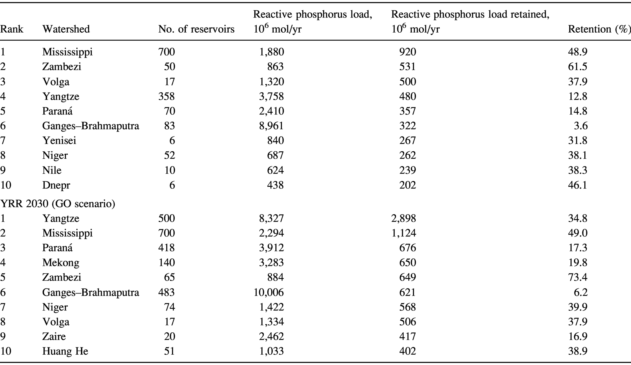
4.3.6.3 Downstream Changes to Temperature and Oxygen
Dam and reservoir management strategies influence water quality within reservoirs and downstream of dams. In this regard, a fundamental consideration is the depth of the reservoir thermocline/oxycline relative to the spillway intake. Many large reservoirs have outflow levels deeper than ~10 m, which is usually below the thermocline, even during warm and dry conditions (Young et al., Reference Young, Kent and Whiteside1976; Winton et al., Reference Winton, Calamita and Wehrli2019). The release of potentially cold, hypoxic, and nutrient-enriched waters can have detrimental consequences to downstream riparian environments. Cooler dam outflow water along the Yangtze River resulted in a delay of fish spawning by several weeks (Zhong and Power, Reference Zhong and Power2015). Macroinvertebrate communities along Guadalupe River exhibited qualities consistent with ecological stress, with reduced diversity and higher numbers of fewer species downstream of Canyon Dam, a deep storage reservoir in the Texas Hill Country (Young et al., Reference Young, Kent and Whiteside1976).
Outflow from large reservoirs is clear and cold with lower oxygen levels. Because of the depth and size of reservoirs, the volume of outflow potentially alters downstream aquatic environments for tens of kilometers. This is shown for two of the larger tributaries to the lower Mekong (i.e., Figure 4.19). Streamflow temperatures varied by four and six degrees (Celcius) 56 km and 78 km downstream of recently constructed dams along the Sesan and Srepok Rivers, respectively (Figure 4.34). The streamflow for both rivers underwent substantial cooling during the dry season, which persisted into the first half of the wet season (May, June, July). Thus, reduced streamflow variability caused by dams occurs with temperature, as it does with water level (stage). The importance of this is highly seasonal and related to the life cycles of aquatic organisms, including fish behavior related to feeding and spawning (Bonnema et al., Reference Bonnema, Hossain, Nijssen and Holtgrieve2020).
Downstream impact of lower Mekong basin dams on water temperature. Comparison of pre-dam (2004–2008) and post-dam (2009–2011) average monthly streamflow temperatures for the (A) Sesan and (B) Srepok Rivers, with dam construction in 2008 and 2009. No major dams were constructed on the (C) Sekong River over the study period, which provides a “control” for comparison. Temperature monitoring stations along the Sesan and Srepok Rivers were 56 km and 78 km downstream of dams, respectively. See Figure 4.19 for location of rivers within the lower Mekong basin.

4.3.6.4 Reservoir Water Quality Management: Tennessee Valley Authority Case Study
The Tennessee Valley Authority (TVA) is a massive federal economic development project in the southeast United States that was initiated during the Great Depression of the 1930s (Figure 4.35). The main focus of the TVA was to build dams for hydroelectricity, flood control, and navigation. The TVA operates forty-nine dams, with twenty-nine built for hydroelectricity and twenty non-power-generating dams with a primary purpose of flood control. The dams are located within the Tennessee River basin (105,900 km2), which drains the southwestern Appalachian Mountains and flows westerly, joining the Ohio River ~40 km upstream of its confluence with the Middle Mississippi to form the lower Mississippi. The Tennessee River is heavily impounded and includes nine main-stem dams and locks that create a 1,050-km long navigable corridor. The approach to reservoir management upon completion of the dams was to maximize hydropower, which resulted in storage and release schedules that did not coincide with riparian ecosystems; essentially the opposite of environmental flows.
Map of the profile of the Tennessee River, showing locations of TVA dams and drainage network of the Tennessee River basin. Unit conversion: 1 mile = 1.6094 km, 1 ft = 0.3048 m.

Reservoir outflow for many dams built by the TVA had poor water quality that did not meet established environmental standards (Table 4.12). A study of twenty dams found that over a thirty-six-year period, downstream flow volumes were too low to support critical riparian functions of aquatic habitat (Higgins and Brock, Reference Higgins and Brock1999). The downstream distance where streamflow volumes were too low exceeded 20 km for ten dams. The Holston River downstream of Cherokee Dam has an average discharge of 130 m3/s, but for a distance of 76 km below, the dam only averaged a minimum flow of 2 m3/s. This effectively resulted in a dry channel bed, although the region has among the highest annual rainfall totals in the continental United States. Additionally, sixteen of the TVA dams had outflow with dissolved oxygen levels below environmental standards (Table 4.12). The French Broad River, downstream of Douglas Dam, had average minimum dissolved oxygen levels of just 0.9 mg/L for an average of 113 days per year over a distance of 129 km downstream of the dam (Higgins and Brock, Reference Higgins and Brock1999). Such low levels of dissolved oxygen represent hypoxic conditions that can be fatal to immobile benthic macroinvertebrates while fish abandon the segment. The river effectively becomes a riparian dead zone.
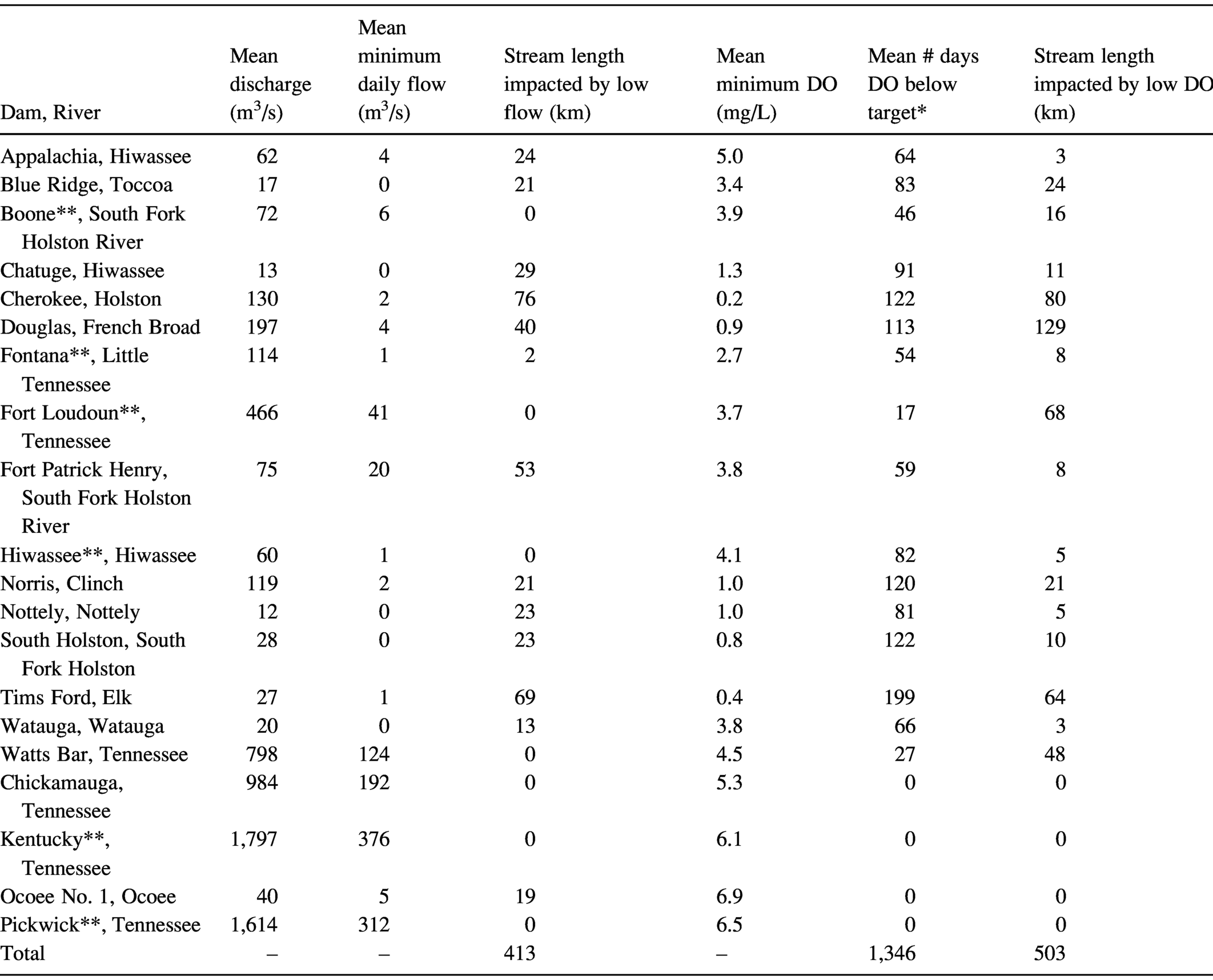
Note: Based on daily streamflow (m3/s) and weekly DO (mg/L) data from 1960 through 1996. Data affected by release improvements were omitted.
* DO target is 6.0 mg/L for nine dams with cold water downstream fishery, and 4.0 mg/L for eleven dams with warmwater downstream fishery.
** Tailwaters not impacted by low flows due to backwater from downstream reservoirs.
Fortunately, in 1991 the TVA initiated changes to its reservoir management strategy to improve downstream ecological conditions (Bednarek and Hart, Reference Bednarek and Hart2005). To increase the wetted surface area of the channel bed, measures included turbine pulsing to create a steady outflow, increased minimum flow volumes, and construction of low weirs downstream to maintain water levels at critical heights. To increase dissolved oxygen levels, modifications were made that involved injecting oxygen into reservoir water as well as structures immediately below the dam to create turbulence and aeration of reservoir outflow water. The measures were largely deemed effective, and both abiotic and biotic conditions improved downstream of the dams. Average dissolved oxygen levels increased by ~34%. The average increase in minimum velocity and discharge was 59% and 528%, respectively. While it was difficult to discern the importance of increased flow velocity relative to increased dissolved oxygen, macroinvertebrate assemblages significantly improved across the study segments. The number of macroinvertebrate families increased by 36% and there was a 13% reduction in the number of macroinvertebrates tolerant of low water quality conditions (Bednarek and Hart, Reference Bednarek and Hart2005).
Downstream rehabilitation of impounded rivers by modifying dam and reservoir operations is critically important because of increased stressors of land cover change and climate change, and because many dams will effectively remain a permanent component of the riparian landscape. But designing reservoir outflow for environmental flows remains a work in progress (Bednarek and Hart, Reference Bednarek and Hart2005; Rader et al., Reference Rader, Voelz and Ward2008; Kunz et al., Reference Kunz, Senn, Wehrli, Mwelwa and Wüest2013). While the efforts of the TVA to improve the downstream environmental integrity of riparian environments were deemed somewhat successful, the TVA’s highly regulated rivers far from resemble a natural stream, and restoration was not the goal. Riparian ecologists have developed an intricate knowledge of critical life cycle phases of stream biota and their relation to abiotic components (e.g., bed material, flow velocity, depth, temperature). Such knowledge has resulted in conceptual models that provide useful signposts to guide river managers in environmentally effective dam and reservoir management, including lateral connectivity with floodplains (Ward and Stanford, Reference Ward and Stanford1995). The actual success of such mitigation measures, however, varies greatly. In view of each river and reservoir representing a unique combination of natural and human controls, such management measures are only likely to be effective with a detailed knowledge of the local fluvial environment (Robinson et al., Reference Robinson, Uelinger and Monaghan2003).
4.4 Dam Removal
The dam paradigm in North America, western Europe, and some of Australia is dam removal.
4.4.1 Drivers of Dam Removal
Dam removal is increasingly viewed as a vital tool in river restoration and is initiated by a variety of drivers (Pohl, Reference Pohl2002; Lejon et al., Reference Lejon, Renöfält and Nilsson2009; Magilligan et al., Reference Magilligan, Graber, Nislow, Chipman, Sneddon and Fox2016; Ding et al., Reference Ding, Chen, Ding and Tao2018). The main driver to remove dams is environmental, initiated by recognition of adverse impacts on rivers and associated environments (Table 4.13). The most important environmental justification for dam removal is to restore connectivity to support and restore fish habitat. Despite the strong interest in increasing aquatic ecosystem habitat, however, ecological justifications are not always singularly sufficient to bring down a dam. Other drivers of dam removal include safety, economics, and cultural heritage and aesthetics (Table 4.13). Free-flowing rivers are valued by society for their own sake, and thus aesthetics are also deemed to be an important motivation for dam removal. Most dam removal projects involve at least a couple of drivers. The high-profile case of the Elwha Dam project (Figure 4.36), for example, was driven by a combination of environmental and cultural heritage issues related to indigenous people and their connection to fish migration, specifically Pacific salmon.
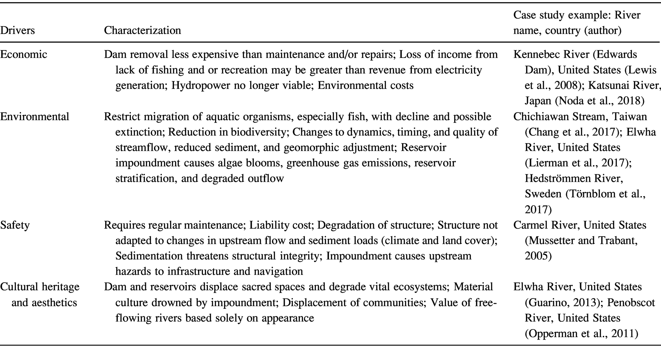
* Most dam removal projects include a combination of drivers. (Author table)
Removal of the 64-m high Glines Canyon Dam on the Elwha River, Washington in February 2012.

4.4.1.1 Legislation and Policy Instruments
Government institutions across international, federal, state/provincial, and local scales have varying types of policy instruments that pertain to specific drivers of dam removal. The U.S. Clean Water Act (Sec. 404) and Endangered Species Acts, for example, are federal legislative tools that can be used in environmentally motivated dam removal ‘projects’, although they are seldom employed (Bowman, Reference Bowman2002; Doyle et al., Reference Doyle, Stanley and Harbor2003b; Opperman et al., Reference Opperman, Royte, Banks, Day and Apse2011). The relicensing of a dam requires a review of the Endangered Species Act as it pertains to adverse environmental impacts as well as measures to manage and mitigate adverse impacts to riparian environments. Sweden has the federal Environmental Objective, which identified sixteen ecosystem goals to be attained by 2020. This included a stated priority of maintaining healthy rivers, lakes, groundwater, and wetlands, among others. A specific facet of the objective was to restore 25% of valuable rivers by 2010, a stimulus for dam removal efforts in Sweden based on environmental justifications (Lejon et al., Reference Lejon, Renöfält and Nilsson2009). For rivers that intersect international borders it is important to have international agreements and institutions to specify cooperation in support of healthy rivers.
The European Union’s Water Framework Directive (WFD) requires that all EU nations manage water in the context of sustainability. Indeed, Article 4 of the WFD includes specific ecologic and hydrologic targets that nations are supposed to attain by 2027 (Directive 2000/60/EC). To adapt to the WFD, the EU developed the River Basin Management Plan as a common strategy with specific deadlines to meet each of the WFD requirements. While the requirements were in accord with the concept of dam removal to improve riparian health, a number of nations did not view the WFD in these terms and were slower to pursue dam removal projects. The implementation and enforcement of the EU’s WFD in the context of dam removal was recently strengthened (May 2020) by the EU Biodiversity Strategy for 2030. The Biodiversity Strategy requires restoration of at least 25,000 linear km of rivers to a free-flowing state through the removal of barriers (dams and weirs), in addition to floodplain and wetland restoration.
4.4.1.2 Economics and Dam Removal
Economics is a vital driver of dam removal and includes multiple facets. While revenue associated with electricity generation is often an important primary consideration for hydropower dams, other economic considerations include revenue associated with tourism and recreation, land use and associated income generation, property values, taxes, fisheries production, sediment management, and dam maintenance and repair (Lawson, Reference Lawson2016). Dam removal projects include formal cost–benefit analyses, which compare the cost of removal to the economic benefits of removal as well as the cost of alternatives to dam removal. Alternatives to dam removal often include the cost of upgrading to meet new standards as regards safety, mechanical and electrical generation, and environmental mitigation, particularly fish passages. The alternatives to dam removal are often twofold higher than the cost of dam removal (Lawson, Reference Lawson2016). Sediment management (discussed below) is usually the most expensive part of dam removal. For some dams, changes to residential property values can be a larger consideration. In some instances, property values increased after dam removal for rivers in Maine and Wisconsin (United States), although it depends on the proximity to the river (Lewis et al., Reference Lewis, Bohlen and Wilson2008; Provencher et al., Reference Provencher, Sarakinos and Meyer2008; Auerbach et al., Reference Auerbach, Deisenroth, McShane, McCluney and Poff2014; Lawson, Reference Lawson2016). And each economic factor may be used to make a case for or against dam removal depending on the competing stakeholders (Morris and Fan, Reference Morris and Fan1998; WCD, 2000; Heinz Center, 2002).
After a decades-long dispute about removing four dams along a 225 km stretch of the lower Snake River, Washington (Ice Harbor, Lower Monumental, Little Goose, and Lower Granite dams) that provide power, flood control, water for irrigation, and navigation, but only about 5% of the regional electricity, the U.S. EPA in 2020 decided not to remove the four dams. The stated reason was concern that a loss of power generation would increase electricity rates for consumers. Earlier economic analyses had shown a net benefit of $310 million, and that the river recreation gains actually exceeded lost revenue from reservoir recreation (Loomis, Reference Loomis2002). The dams ensure ~450 km of navigation from the Pacific Ocean at the mouth of the Columbia River to Lewiston, Idaho. But the dams are also associated with steep decline in Pacific salmon stock as well as declines in species that heavily rely upon salmon for feeding, which includes Southern Resident killer whales.
Globally, numerous dams are older than five decades (e.g., Figure 4.4) and in need of costly repairs, maintenance, and upgrading (Morris and Fan, Reference Morris and Fan1998; Heinz Center, 2002; Doyle et al., Reference Doyle, Stanley and Havlick2008). The average age of US dams is fifty-seven years (as of 2020), and over 10,000 dams (>2 m) are older than seventy years (e.g., Figure 4.8). The cost of upgrading and repairing such infrastructure is enormous, and was estimated in 2016 at about $65 billion (Table 4.14). Because there are so many old dams with questionable structural integrity, an additional strong motivation for dam removal is liability, which ultimately relates to economics (Heinz Center, 2002). Most dams are locally owned and many owners are increasingly opting for dam removal to avoid expenses associated with liability or repairs. Small dam removal projects often cost less than the cost of safety repairs (Born et al., Reference Born, Genskow, Filbert, Hernandez-Mora, Keefer and White1998; Bowman, Reference Bowman2002). Thus, the same rationale for the original construction of dams – economics – is now being utilized to justify their removal.

4.4.2 Stakeholders and Dam Removal
Getting different stakeholders to work together to accomplish a common goal is always challenging, and is a core element of “integrated water resource management” (Lejon et al., Reference Lejon, Renöfält and Nilsson2009; Opperman et al., Reference Opperman, Royte, Banks, Day and Apse2011). Stakeholder types involved in dam removal projects potentially include energy companies, recreational and commercial fishing organizations, environmental organizations, indigenous peoples, cultural heritage preservationists, property owners, developers and the business community, and governmental organizations at local, state/provincial, federal, and international scales. In North America, indigenous peoples are important stakeholders in dam removal efforts, particularly coastal communities whose livelihoods are linked to fisheries impacted by dams. Some environmental organizations are explicitly oriented to dam removal, such as International Rivers, American Rivers, and DamRemoval.eu.
Stakeholder involvement in the dam removal process should occur at all stages of the project. Success requires that all stakeholders be immersed in plans and progress as the project evolves. As much as general “lessons learned” are important, the reality is that all dam removal projects are different (Stanley and Doyle, Reference Doyle, Harbor and Stanley2003). Each project has unique cultural, political, and historical dimensions that impact the outcome. Although government agencies and scientists may be in support of dam removal, opposition from local stakeholders can result in the failure or extensive delay of a seemingly well-intended project (Born et al., Reference Born, Genskow, Filbert, Hernandez-Mora, Keefer and White1998; Lejon et al., Reference Lejon, Renöfält and Nilsson2009; Fox et al., Reference Fox, Magilligan and Snedden2016; Magilligan et al., Reference Ma, Nittrouer and Naito2017). Regionally, there can be great differences in the representation of different stakeholder types, and whether they have favorable or negative views of dams. In western portions of North America, a mill dam over a hundred years old may be considered valuable “cultural heritage” by some stakeholders, while in Europe structures of that age may seem less unique.
4.4.3 International Extent of Dam Removal
4.4.3.1 Dam Removal in North America
Dam removal is occurring at an accelerated pace and being guided by increasingly sophisticated procedures and monitoring conventions, although there is great regional and national and international variability across the United States, Canada, and Mexico.
In total, 1,699 dams were removed in the United States between 1900 and 2019 (Figure 4.37). And 806 dams were removed over the past decade, nearly double the previous decade. Most dams removed are less than 5 m in height. In the United States, the hotspots for dam removal are in the northeast, northwest, and the northern Midwest (American Rivers, 2020). Numerous mill dams in New England have been removed. Many of these are well over a hundred years old and represent the region of the most intense and oldest river impoundment in the United States (Walter and Merritts, Reference Walter and Merritts2008). The largest dam removal project in New England is the Great Works Dam in 2012 and the Veazie Dam in 2013 along the lower Penobscot River (22,196 km2) in Maine. The project also included modification to dam structures to create fish passages, and was driven to restore some 3,200 km of riparian habitat to anadromous fish, such as Atlantic salmon (Salmo salar), alewife (Alosa pseudoharengus), American shad (Alosa sapidissima), and Atlantic sturgeon (Acipenser oxyrinchus oxyrinchus). And it worked, as fish populations quickly returned within a few years, with anadromous fish species increasing while slower lacustrine species declined (Watson et al., Reference Watson, Coghlan, Zydlewski, Hayes and Kiraly2018). California had twenty-three dams removed in 2019, and Pennsylvania had fourteen. Texas had one dam removed in 2019, and has only had eight in total removed. The paucity of dam removal projects in Texas is concerning because it has the highest number of dams and the largest proportion of its surface water impounded of any state in the United States (Graf, Reference Graf1999).
US dam removal between 1900 and 2019. Total dams removed are 1,699 (May 22, 2020). Dam removal between 1900 and 1979 grouped in twenty-year periods and from 1980 to 2019 by decade.

In terms of height, 349 dams that are higher than 5 m have been removed in the United States. In the Pacific Northwest, dams are being removed in smaller coastal draining rivers where it is mainly about restoration of Pacific salmon habitat (all five species), which quickly return to spawn in upstream rivers for the first time after many decades (Lierman et al., Reference Ma, Nittrouer and Naito2017). The largest dam removal project in the world – to date – occurred along the Elwha River (820 km2) in the Olympic Peninsula of coastal Washington over a couple of years (see discussion below). The removal project occurred in two phases, the 33-m Elwha River Dam in 2011 followed in 2012 by a phased removal of the 64-m Glines Canyon Dam (Ritchie et al., Reference Ritchie, Warrick and East2018).
Dams are also being removed in Canada, although at a slower pace than the United States. The removal of small dams in Canada is tempered by the fact that large dams have recently been completed and are still being constructed along major waterways. Since 2006 twenty-one dams have been removed in British Columbia, including four large dams >9 m in height. Dam removal is proceeding within established removal procedures and guidelines. A positive sign that dam removal is becoming a mature environmental industry in Canada is that sophisticated guidelines are being developed within clear policy frameworks at the scale of individual provinces. Ontario, for example, has the Lakes and Rivers Improvement Act (LRIA) that specifically includes a range of fluvial geomorphic criteria to develop a dam removal plan, including sedimentary and morphologic adjustments (Ontario Ministry of Natural Resources, Reference Dettinger2011).
In Mexico, dam removal is not occurring with any documented frequency. Indeed, the trend is somewhat the opposite and several large dams were constructed in the 2000s. In 2020, Mexico confirmed it will go forward with the massive Chicoasén II hydroelectric dam (240 MW) in the deep canyons of the Grijalva River in the mountainous southern state of Chiapas. The dam is the second phase of a larger hydroelectric site that includes the 261-m high Manuel Moreno Torres (Chicoasén) Dam, the tallest dam in North America. Several other proposed Mexican dams, fortunately, have been stalled or canceled over the past decade because of substantial opposition from environmentalists, human rights supporters, and indigenous peoples.
4.4.3.2 Dam Removal in the European Union
Dam removal in the European UnionFootnote 3 is occurring with much greater frequency over the past decade, with France leading the way (Fernández Garrido, Reference Fernández Garrido2018; Schiermeier, 2018). The increasing pace of dam removal is occurring for several key reasons, including: (1) The European Union Water Framework Directive (WFD), which requires free-flowing rivers to attain good ecological status by 2027 (noted above); (2) environmentally oriented national strategies supported with science that view river networks as linked to landscapes; and (3) the development of effective nongovernmental organizations that champion the cause of dam removal. Nevertheless, like the United States there is considerable regional variability in the pace of dam removal. Many of the debates and the roles of stakeholders with regard to dam removal projects are similar to the United States (Born et al., Reference Born, Genskow, Filbert, Hernandez-Mora, Keefer and White1998; Lejon et al., Reference Lejon, Renöfält and Nilsson2009; Jorgensen and Renofalt, Reference Jorgensen and Renofalt2013; Magilligan et al., Reference Ma, Nittrouer and Naito2017). To obtain a clearer picture of dam removal across the EU it is crucial that a standard system of data reporting is developed.
A recent “fitness check” of the effectiveness of implementation of the EU Water Framework Directive revealed that the quality of some 40% of European rivers is under “hydromorphological” stress caused by dams and hydraulic engineering (EEA, 2018; EC, 2019). This recognition further increased attention to the issue of dam removal, as well as passage in 2020 of the EU Biodiversity Strategy for 2030 that includes a stated purpose to greatly increase the length of free-flowing rivers in Europe. Dam Removal Europe (damremoval.edu) is the key NGO, and has singularly focused on removing barriers (dams and small weirs) that are obstacles to fish migration, which like North America, is the primary driver of dam removal. A recent development (as of 2018) is the formation of AMBER (Adaptive Management of Barriers in European Rivers), a consortium of twenty key private and public specialists that represent a range of stakeholders involved with dam removal in Europe. AMBER includes partners from the hydropower industry, river authorities, nongovernmental organizations, and university scientists with the intention to enhance collaboration and knowledge transfer about the process of dam removal. An important task being undertaken by AMBER is to arrive at a tally and site-specific characterization of dam removal projects, which is difficult because of different protocols for reporting, as noted for Spain. Additionally, an important element of AMBER is “citizen science,” which directly involves the public in data collection and dissemination. Combined, these two thrusts of European dam removal have increased the visibility of the topic to a range of public and private stakeholders, increasing public participation in the process of dam removal.
According to the DamRemoval.eu NGO, some 5,000 dams (and weirs) have been removed across five European nations as of 2018. This includes France with 2,425 dam removals (partially removed obstacles: 5,728), Sweden with >1,600, Finland with >450, Spain with >250, and Great Britain with 156 dam removals (Fernández Garrido, Reference Fernández Garrido2018). Many EU nations have ambitious plans for dam removal that link national strategies with the EU WFD. Among the several significant dams removed in Europe are the Retuerta dam (14 m) and the La Gotera dam (8 m) in the Duoro basin (Spain) in 2013 and 2011, respectively. The latter was initiated as part of the Spanish National Strategy of River Restoration to increase hydrologic continuity through the Alto Bernesga Biosphere Reserve of the Man and Biosphere Programme. In France’s nationally symbolic Loire basin, the Saint Etienne du Vigan dam (14 m) on the Allier tributary and the Maisons Rouges dam (4 m) on the Vienne tributary were both removed in 1998 as part of the French governments “Plan Loire Grandeur Nature.” The main focus is to increase fish migration to the upper basin headwaters, particularly for spawning of Atlantic salmon (Salmo salar). The largest dam removal project in Europe occurred along the Sélune River in Normandy, France. The 36-m high Vezins Dam was the first of two dams to be removed (2019), with the second being the 15-m high La Roche Qui Boit removed in 2021. Combined, the removal of the two dams reopen 91 km of a coastal draining river to migrating Atlantic salmon, eels, and other riparian wildlife, which empties into the bay of Mont-Saint-Michel – a UNESCO world heritage site and key stakeholder related to cultural heritage.
Although progress is being championed in scientific media (Schiermeier, Reference Schiermeier2018), dam removal varies greatly across the European Union. And it often varies within individual nations between states/provinces or basin, as with the issue of data reporting in Spain. Data reporting procedures in Spain are not centrally coordinated and instead are organized at the scale of the larger drainage basins, which vary considerably in format and in public accessibility (Rincón Sanz and Gortázar Rubial, Reference Rincón Sanz and Gortázar Rubial2016). In the Douro River basin (98,400 km2), for example, 116 dams and barriers were removed between 2009 and 2016, the highest in any basin in Spain. Of these dams, 31 were <2 m height, 16 were 2–5 m height, 2 were >10 m height, but 67 of the dams removed in the Duoro basin did not include a recorded dam height or descriptive information (Ministry for Ecological Transition, MITECO, 2020). In comparison to the Duoro Basin, which has 145 large dams, the Ebro River basin (80,093 km2) is the most impounded in Spain, and has 299 large dams. But data from the Ebro River basin authority only reported 5 dams removed (Rincón Sanz and Gortázar Rubial, Reference Rincón Sanz and Gortázar Rubial2016).
4.4.4 Science of Dam Removal
Effective dam removal is the essence of multi- and interdisciplinary science, and commonly includes consultation with engineers, earth scientists, biologists, economists, archaeologists and historians, social scientists, among others. While the science is important, however, specific scientific activities need to be intricately synchronized with the legal and policy framework in which dam removal projects exist (Aspen Institute, 2002; Bowman, Reference Bowman2002; Heinz Center, 2002; Doyle et al., Reference Doyle, Stanley and Harbor2003b; USSD, 2015; Randell and Bountry, Reference Randle and Bountry2017).
Depending on the size and sensitivity of the riparian area, the time required to remove a dam can vary greatly, with even modest-sized dams (~5 m) frequently taking a decade or two to remove. This is largely because of requirements to obtain a range of permits and the importance of having conducted research on the potential impacts of the prospective dam removal project (USSD, 2015). This is particularly the case when dam removal projects may degrade wetlands, if the riparian area includes endangered species or other important ecosystems, or if valuable cultural materials are associated with downstream riparian area as well as the dam and reservoir structure. Smaller dams and weirs without such critical habitat concerns are often (but not always) less complicated to remove, particularly smaller run-of-river structures that store little sediment. In such cases, the removal process is often regulated at the state or provincial level. Indeed, many states and provinces have detailed guidelines and “checklists” for how landowners can remove smaller structures (i.e., Ontario Ministry of Natural Resources, Reference Dettinger2011). The removal of small dams and structures as a community-based program has also proven effective at restoring aquatic habitat, particularly if effectively coordinated by a larger government agency (Lenhart, Reference Lenhart2003). Regardless of reservoir size, however, legal disputes between different stakeholders can significantly delay (by decades) or completely stymie a dam removal project.
Dam decommissioning is expensive. Dam removal cost widely varies according to the scope and sensitivity of the project (Aspen Institute, 2002; Randle et al., Reference Randle, Morris and Whelan2019). Funding may come from a variety of sources, such as private power companies, environmental organizations, and government agencies at international, national, state/provincial, and local scales. It is essential to establish stakeholder responsibility for cost early in the exploratory phase, as cost can escalate. Morris and Fan (Reference Morris and Fan1998) report that the largest proportion of dam removal cost is associated with sediment management – at 48%. The actual removal of the hydraulic infrastructure and environmental engineering are 30% and 22%, respectively. And if the dam removal project includes substantial polluted reservoir deposits, the sediment management cost significantly increases (Evans, Reference Evans2015).
The science of dam removal is rapidly developing into a sophisticated and diverse enterprise. This is largely because of (1) being able to draw upon a rich theoretical foundation of knowledge in fluvial dynamics and aquatic ecosystem processes developed over past decades, (2) increasing availability of historic datasets, and (3) sophisticated monitoring and data collection equipment.
The specific research activities associated with a dam removal project should be organized within a temporal–spatial framework that includes a pre-dam-removal phase, removal phase, and post-dam-removal phase that spans upstream (control site), dam and reservoir, and downstream reaches. The latter may also include shallow marine and beach environments for river basins tightly coupled to coastal dynamics.
Most dam removal projects begin by establishing specific hydrogeomorphic and biological reference targets, which may be historic prehuman disturbance “baseline” conditions (if possible to establish) or other environmental targets mutually agreed to by relevant stakeholders (Aspen Institute, 2002; Heinz Center, 2002; Stanley and Doyle, 2003; USSD, 2015). In practice, many datasets for reference conditions (prior to dam construction) may extend back only about a decade. In such cases, it is ideal that this includes both a downstream and upstream control reach (above reservoir backwater).
Although a return to a natural riparian regime and the replenishment (reactivation) of stored reservoir sediments to downstream reaches is a common goal, the most important task is to assess the potential impacts of an abrupt sediment pulse to downstream physical and biological habitat. Thus, a key element to dam removal planning is to develop a sediment management strategy (Figure 4.38) that outlines the sequence of procedures according to varying qualities of reservoir deposits (Randle et al., Reference Randle, Morris and Whelan2019).
Steps for removal of reservoir sedimentary deposits. Sequence largely depends upon environmental concerns related to reservoir deposits.

4.4.4.1 Managing Reservoir Sediment Removal
Reservoir drawdown is a crucial step in dam removal, and management of sedimentary deposits during dam removal follows a sequence of specific steps (Figure 4.38). The method of drawdown is of key importance to sediment mobilization during and after reservoir drawdown. Rapid reservoir drawdown results in considerable hydraulic flushing and scour of reservoir deposits (Scheueklein, Reference Scheueklein1990), and produces a large sediment pulse that can be detrimental to downstream riparian environments (Grimardias et al., Reference Grimardias, Guillard and Cattanéo2017). A slower drawdown is more benign to downstream riparian environments, although it can result in a larger volume of reservoir deposits that are disconnected from active fluvial processes. Additionally, upon drawdown a sharp knickpoint forms near the dam base (Neave et al., Reference Neave, Rayburg and Swan2009). Subsequent upstream headcut migration of the knickpoint through reservoir deposits further removes sediment by triggering mass wasting and erosion of noncohesive deposits (Morris and Fan, Reference Morris and Fan1998; USSD, 2015).
Because reservoir deposits sequester large amounts of phosphorus and nitrogen from upstream agricultural landscapes (Maavara et al., Reference Maavara, Parsons and Ridenour2015), the release of nutrients into the active fluvial system and eventually into downstream coastal waters is a concern during the dewatering phase of dam removal (Riggsbee et al., Reference Riggsbee, Wetzel and Doyle2012).
Many dams impound polluted reservoir deposits and it is important that dam removal does not result in contaminated sediment pulses impacting downstream environments (Evans, Reference Evans2015). Sediment pollution from dam removal is of particular concern in reservoirs downstream of old industrial and mining areas (Tullos et al., Reference Tullos, Collins and Bellmore2016). In such cases, removal of contaminated deposits must precede dam removal, or dam removal may be untenable. Along the Hudson River in New York, the 1973 removal of Fort Edward Dam resulted in several hundred thousand cubic meters of sediment contaminated with polychlorinated biphenyls (PCBs) to be transported downstream. After decades of legal disputes with industry about whether the polluted sediment should be capped or removed, some 2 million m3 of sediment was eventually dredged from the river bed, in addition to floodplain restoration, at a cost of $561 million (Evans, Reference Evans2015). And legal disputes between the state of New York and industry are ongoing as to whether the polluted sediment has been satisfactory removed.
4.4.4.2 Removal of Toxic Reservoir Deposits
The Milltown Dam removal project along Clark Fork (59,320 km2), the largest river in Montana, included reservoir deposits polluted with arsenic, copper, and other metals associated with a legacy of mining (Sando and Vecchia, Reference Sando and Vecchia2016). The dam had been constructed in 1907 and within months an enormous flood (~500-year RI) deposited tons of polluted sediment into the reservoir (Evans, Reference Evans2015). The reservoir is part of Clark Fork Basin Superfund Complex, the largest superfund site in the U.S. (U.S. EPA, 2016). The environmental and health problems associated with the contaminated deposits had been known since the early 1980s when residents started to become ill from polluted drinking water. The issue came to a head in the winter of 1996 when a large ice jam threatened to breach the dam. To prevent Milltown dam from being damaged by the ice jam the reservoir water level was lowered. But the reservoir drawdown was too abrupt and resulted in hydraulic scour of polluted reservoir deposits, releasing a toxic pulse that resulted in a massive fish kill downstream (Diamond, Reference Diamond2006; Evans, Reference Evans2015). Prior to finally dismantling the 12.8 m tall dam in spring 2008 (initial breach March 28), some 2.2 million m3 of polluted deposits (40% of total reservoir volume) were hauled away by train and buried outside of the riparian zone (U.S. EPA, 2016). By far the largest proportion of the Milltown Dam removal cost was managing reservoir sediment removal ($120 million).
The environmental disaster associated with the abrupt 1996 drawdown of the Milltown dam on Clark Fork River provided a useful lesson employed in the dam removal strategy. Rather than an abrupt drawdown, reservoir drawdown occurred very slowly over nearly two years, extending from June 1, 2006 to the dam breach, on March 28, 2008. While arsenic levels increased during the drawdown, it increased much less than copper (Figure 4.39). Nevertheless, despite the attempt to limit pollutant mobilization during the drawdown, the increased suspended sediment concentrations during the drawdown period (June 2006–March 2008) flushed 140,000 metric tons of particulates, which included 44 tons of copper and 6.4 tons of arsenic eroded from the reservoir. This is interesting because it shows that even when exercising great caution with reservoir drawdown, it should reasonably be expected that fine-grained deposits will be hydraulically excavated from the reservoir. Additionally, higher sediment loads during the drawdown phase were also attributed to structural landscape modifications (roads, facilities, excavation, etc.) associated with preparation of dam removal. Following the dam breach, an additional 420,000 tons of suspended sediment were transported downstream, which included 15.8 tons of arsenic and 169 tons of copper. A discharge of 250 m3/s during the removal phase resulted in a sediment load of 20,000 while several months later the same discharge produced a sediment load of about 2,000 tons (Sando and Lambing, Reference Sando and Lambing2011). Overall, copper, arsenic, and suspended sediment decreased by 53%, 29%, and 22%, respectively, between the start of water year 1996 and the end of water year 2015 (Sando and Vecchia, Reference Sando and Vecchia2016).
Arsenic, copper, and suspended sediment between 1996 and 2015 for Clark Fork River. Sampling was 4.8 km downstream of Milltown Dam. Note: y-axis is logarithmic (USGS station i.d.: 12340500).

4.4.4.3 Reworking of Reservoir Deposits
To evaluate changes to fluvial sediment budgets associated with dam removal it is necessary to calculate downstream sediment loads associated with the reworking of reservoir deposits. Sediment mass (tons) is commonly estimated from the volume (m3) of reservoir deposits (Randle and Bountry, Reference Randle and Bountry2017). Accurate sediment load estimates from reservoir deposits require data on the weight of specific particle size classes, and whether they are subaqueous (submerged) or subaerial (above the water surface) deposits. This data is obtained from reservoir sedimentation surveys that measure the bathymetry and topography of reservoir deposits, as well as the particle size distribution obtained from borings and geophysical mapping (Yang, Reference Yang2006).Footnote 4 The weight of fine-grained deposits varies considerably according to whether it is submerged or above water (Table 4.15). Additionally, cohesive deposits, such as clay, substantially compact over time, which reduces pore space and increases sample weight. For example, after fifty years of compaction clay loses 35% of its original volume (Figure 4.40), which also increases reservoir storage capacity.
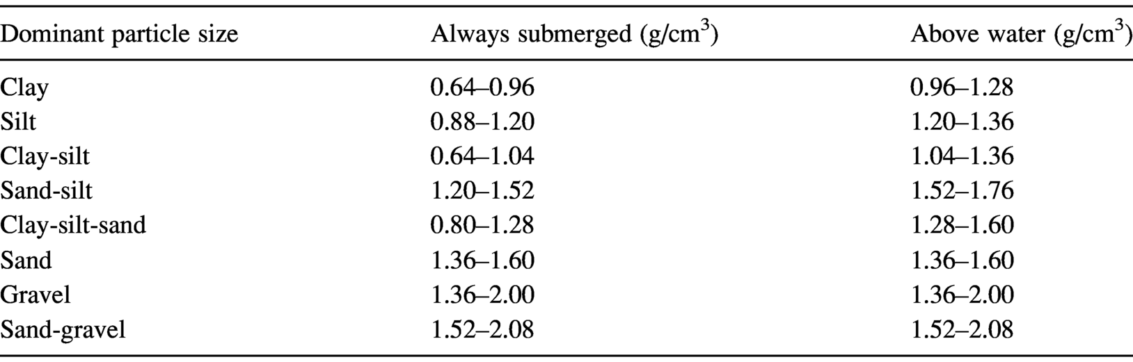
Reservoir sediment compaction over time for different particle size classes over one hundred years. Values are for continuously submerged deposits. Sand not shown because of minimal consolidation.

Most reservoir deposits reassimilated into the active fluvial system are eroded within the first year or two of dam removal, particularly for smaller elongated reservoirs with coarse deposits (Major et al., Reference Ma, Nittrouer and Naito2017). After the first couple of years, the amount of reservoir sediment reworking abruptly decreases as the channel stabilizes and as reservoir deposits become anchored with vegetation. A review of twenty-one dam removal projects in the United States (Table 4.16) revealed that over 40% of reservoir deposits were reworked and resupplied to the active fluvial system within the first year of dam removal by moderated streamflow events (Major et al., Reference Ma, Nittrouer and Naito2017). The proportion of reservoir deposits that eventually become assimilated back into the active sediment regime varies according to several factors, including sediment texture (fine or coarse), lateral channel dynamics, flood regime, and the size of the reservoir relative to the river channel. The amount of reservoir reworking appears to be less for broader reservoirs with finer-grained deposits and less lateral channel activity (Doyle et al., Reference Doyle, Harbor and Stanley2003a), although more documentation of dam removal projects is needed across lowland settings with fine-grained reservoir deposits.
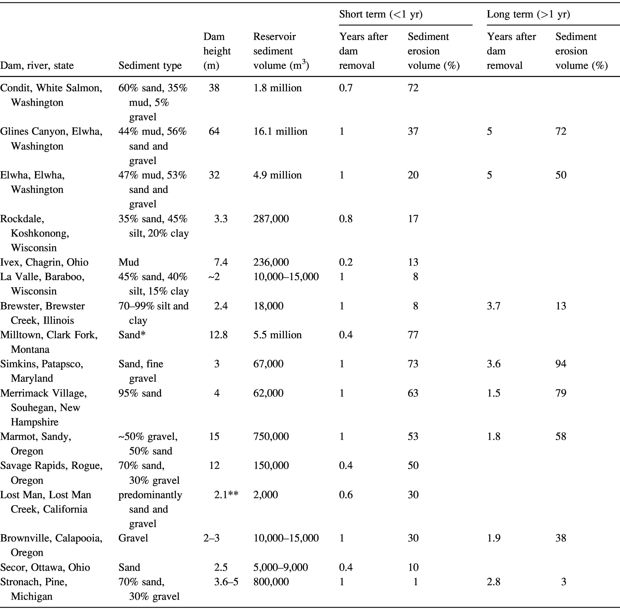
* Approximately 40% of sediment excavated prior to dam breaching was part of Superfund remediation efforts.
** Dam height from Sacklin and Ozaki (Reference Sacklin and Ozaki1988).
An additional factor that influences reservoir sediment reworking includes the biogeographic regime relative to the seasonality of reservoir drawdown (Cannatelli and Crowe-Curran, Reference Cannatelli and Crowe-Curran2012). If vegetation quickly colonizes reservoir deposits following reservoir drawdown, sedimentary deposits can effectively remain “locked in place” within the old reservoir site. This can be a desirable outcome. If not, vegetation may have to be removed to increase the possibility of sediment reworking (Bountry and Randle et al., Reference Randle and Bountry2017). Channel incision within the reservoir deposits forms anthropogenic terraces, reducing the possibility of erosion and reworking during flood events. Additionally, some reservoir sediments deposited atop natural terraces are unlikely to be hydrologically connected during subsequent flood events. In some cases, temporary training dikes can steer laterally active channels toward reservoir deposits to increase their potential for erosion. Fine-grained reservoir deposits distributed across wide valleys are less likely to be reassimilated into the active fluvial system.
4.4.5 Post Dam Removal Response
Comparisons of before, during, and after field data from biological sampling, sediment sampling, and morphologic measurements illustrate the influence of dam removal to riparian environments. Downstream environments adjust and recover to sediment pulses produced by dam removal usually within a few years, particularly fish populations. While there are few adverse consequences to aquatic ecosystems after dam removal, benthic organisms may require additional time to become reestablished (Doyle et al., Reference Doyle, Harbor and Stanley2003a). Biological assemblages may be different than pre-dam assemblages because of environmental changes having occurred since impoundment (Foley et al., Reference Foley, Warrick and Ritchie2017).
Bed material usually becomes finer following dam removal. This occurs for two reasons. Firstly, the influence of impoundment usually results in winnowing of fine deposits so that the channel bed material becomes coarser. Secondly, finer reservoir deposits are more easily mobilized and flushed downstream than the coarser deposits, which moves downstream as a slower wave of coarse deposits. The interstitial pore spaces of the channel bed active layer may initially become clogged with fine sediments (the embeddedness problem) immediately downstream of the former dam site, decreasing with distance to perhaps tens of kilometers downstream. This is a key consideration and represents a direct form of aquatic habitat degradation that can be important to benthic macroinvertebrates and fish spawning. Even several centimeters of embeddedness over a few months can be detrimental to the benthic habitat of aquatic organisms, and of crucial concern if the species is endangered. This again highlights the importance of the timing of dam removal, as the streamflow variability following dam breach is critical to mobilization and downstream assimilation of reservoir deposits into the active sediment load. Downstream fining of bed material is not always obvious. Downstream of two small dams removed in Wisconsin, the reworking of fine-grained reservoir deposits (muddy sand) did not result in appreciable change in downstream bed material size (Doyle et al., Reference Doyle, Stanley and Harbor2003b).
The downstream channel morphology adjusts rapidly to dam removal, although it is dependent upon receipt of coarse sediment pulses. Channel bed aggradation is the initial morphologic response after dam removal, with some infilling of pools and aggradation of bars. Minor channel bed incision often occurs after several years as the initial coarse sediment pulse is transported downstream by higher flows. Overall, the particle size of bars increases, and grain size distributions become less well sorted. Some channel cross sections increase width-to-depth ratios, becoming shallower and wider, particularly braided rivers. Increased flow variability results in more frequent lateral connectivity between channel and riparian wetlands, including renewed overbank sedimentation.
4.4.5.1 Elwha River Dam Removal Case Study
The Elwha River dam removal project in the US Pacific Northwest is an ideal “laboratory” to study the impacts of dam removal on geomorphic and related ecosystem processes for a coarse-grained system. This is because it is the world’s tallest dam removal project and occurred on a modest-sized (833 km2, Q-avg. 42.7 m3/s) mountainous (peak 1,452 m elev.) gravel bed river that drains directly to the coast. And Elwha River and Glines Canyon Dams were only 7.4 and 21.6 km upstream of the river mouth at the Juan de Fuca Strait, respectively. Thus, detectable geomorphic and ecological changes to downstream riparian and coastal environments was all but assured. The study includes a range of morphologic, biological, and hydraulic, and sedimentologic sampling within a conventional research framework to capture the disturbance (spatially: upstream, at reservoir, downstream; temporally: before, during, and after).
The Elwha River Dam removal project is an example of stakeholders joining forces to dismantle dams for river restoration. The S’Klallam people of the Salish Indigenous First Nations historically heavily relied upon annual salmon runs in the Elwha basin for prosperity and spiritual wellness. They fought the dams for many decades. By joining with several environmental stakeholders they were able to finally breach the bureaucracy and power of the hydroelectric industry, and bring down the dams. The Elwha River Ecosystem and Fisheries Restoration Act of 1992 was the key legislative piece to trigger the removal of the Elwha River Dams. The Act specified that the Secretary of Interior should purchase the dams to initiate complete restoration of the Elwha River, including its anadromous fisheries.
Removal of the Elwha River dams occurred in stages to minimize the downstream disturbance of the sediment pulse, with reservoir drawdown starting in September 2011. The two dams were removed in phases, with bed material first moving past the breached 32-m Elwha Dam site in spring 2011 and across the breached 64-m Glines Canyon Dam site autumn 2011, although removal of the structures extended to 2014 (East et al., Reference East, Logan and Mastin2018). Over a five-year period (2011–2016) ~20 million tons of reservoir deposits were reworked by lateral channel migration and incision. This was about two-thirds of the total sediment volume stored in the reservoir, which resulted in downstream sediment pulses being some twenty to forty times greater than “natural” annual maximum sediment loads (East et al., Reference East, Logan and Mastin2018).
By 2015, already 90% of the reservoir deposits had been discharged to the coastal zone (Ritchie et al., Reference Ritchie, Warrick and East2018). Only minor amounts of long-term storage of reservoir sediment will occur as overbank deposits, although some sediment storage evidently occurred within side channels (East et al., Reference East, Logan and Mastin2018). The median particle size decreased from cobbles (144–174 mm) before dam removal to gravel (18 mm) by 2013. By summer 2017, particle size had become somewhat coarser to 40 mm (gravel), but was nevertheless considerably finer than before dam removal (Figure 4.41). Because the particle size did not change upstream of the dam (in the control reach), it is concluded that downstream fining of the channel bed occurred because of the reworking of reservoir deposits.
Downstream changes to Elwha River channel before and after dam removal (photos looking upstream). Note changes to particle size of bed material and presence of wood: (A) One week prior to dam removal (September 2011). (B) Eleven months after dam removal, but prior to arrival of main sediment pulse (August 2012). (C) Shortly after sediment pulse (September 2014). (D) Almost six years after dam removal, four years after sediment pulse (July 2017).

Morphologically, the downstream channel reaches adjusted to the pulses by changing from a riffle morphology to a plane-bed morphology. Surveys for downstream channel cross sections showed variable geomorphic response and recovery (East et al., Reference East, Logan and Mastin2018). By spring 2013, the reach averaged bed elevation change ranged from about +0.38 m to +0.82 m of aggradation (Figure 4.42). But already within a few years most of the channel bed aggradation from the initial sediment pulse had been reworked, as channel incision ensued. By summer 2017, the average bed elevation changes at downstream research sites showed a net aggradation, but it had decreased to +0.15 to +0.35 m. These average values mask local-scale geomorphic variability, and channel bars are indeed now a more prominent component of the channel bed environment than prior to dam removal, with some bars +1.0 m. Additionally, the channel thalweg displays greater lateral mobility than previously, with one reach having laterally migrated by about 30 m.
Reach-averaged channel-bed elevation changes between seasonal topographic surveys, referenced to earlier baseline survey data (not shown). Control reach averaged six cross sections spaced along a ~100-m channel segment located 1.5 km upstream of the upper end of Lake Mills (Glines Canyon Dam reservoir). The downstream reach was centered at 1.9 km below Elwha Dam and included six cross sections over a 172 m long channel segment. The two arrows indicate the approximate date when reservoir deposits were first transported past the two breached dam sites (Elwha, left and Glines, right).

Ecological changes followed geomorphic changes after removal of Elwha River dams. Tributary streams above the Elwha River Dam were being recolonized for spawning within a couple years by the river’s iconic fish, Coho salmon (Liermann et al., Reference Liermann, Pess and McHenry2017). At the coast, the copious sediment volumes resulted in about 1 m of vertical aggradation and some 400 m of lateral (deltaic) aggradation (Ritchie et al., Reference Ritchie, Warrick and East2018), which are already being colonized by pioneer vegetation (Foley et al., Reference Foley, Warrick and Ritchie2017). The prograding river mouth is associated with a salinity shift from coastal to more freshwater environments, including fish and macroinvertebrates communities. A number of activities are being conducted by government agencies and environmental organizations, including monitoring of sediment, vegetation, benthic invertebrates, including radio telemetry to map the movements of anadromous fish. The Elwha River dam removal project specifically applies to humid braided rivers (Figure 4.43), although a number of the findings are in accord with dam removal trajectories observed in other settings (Foley et al., Reference Foley, Warrick and Ritchie2017).
Conceptual model illustrating changes in sedimentary and geomorphic regime before, during, and after dam emplacement and dam removal based on the Elwha River dam removal project in the Olympic Peninsula of Washington (United States). (A) Prior to dam emplacement. (B) Dammed river, showing deltaic reservoir sedimentation. Downstream of the dam the river is incising, narrowing, and channel bed material is becoming coarser. (C) Initial post‐dam removal phase (weeks to one to two years), showing braided channel above and below the former dam site with exposed reservoir deposits. Longitudinal profile of water surface and reservoir sediment includes migrating knickpoint. Downstream of the dam, new deposition of finer‐grained sediments buries coarse-grained armored channel bed sediment that characterized the impounded system. (D) Later in the post-dam removal phase (two to ten years), channel incision occurs through reservoir deposits and into initial post-dam removal deposits downstream of the dam.

4.4.6 Synthesis of Dam Removal Results
While returning to a pristine riparian status is not widely championed by river managers and scientists, dam removal is now a key component of the “river restoration” enterprise (Magilligan et al., Reference Ma, Nittrouer and Naito2017). The detailed inventory and analysis of morphologic, sedimentary, hydrologic, and ecosystem data of numerous dam removal case studies provide sufficient resolution for development of a general model of river recovery to dam removal (Figure 4.44). Important differences to consider include the type of reservoir deposits (fine or coarse grained) and the shape and size of the reservoir (long and narrow or wide and shallow). This sets up a key distinction in the response because of the vegetation regime, and the potential to anchor fine-grained deposits “permanently” after dam removal by woody vegetation. Additionally, the reservoir drawdown in relation to the type and environmental condition of reservoir sediments is a key consideration, particularly with regard to the release of stored nutrients with the dewatering phase as well as the release of contaminated sediments into the active system. While fish are a key component of riparian ecosystems, other types of biota such as benthic invertebrates are also important to monitor, and have a slower recovery time than fish. Some benthic organisms may not recover because of broader watershed scale environmental changes to the system. Woody riparian vegetation that quickly colonizes stabilized sedimentary bars and wetlands after reservoir drawdown requires substantial efforts to remove, and may become a permanent condition of the riparian environment.
Conceptual model of river response to dam removal, including abiotic and biotic trajectories. The endpoints of possible outcomes, “best” and “worst,” range from full recovery of riverine geodiversity (physical integrity) and biodiversity to a completely degraded and polluted river associated with contaminated sediment release and a sediment pulse that obliterates channel aquatic habitat.

Drawing upon numerous case studies it can be concluded that dam removal improves downstream riparian geodiversity (i.e., physical integrity) and biodiversity. A couple of decades of research can be summarized with the following points regarding the impact of dam removal on rivers (Aspen Institute, 2002; Heinz Center, 2002; Doyle et al., Reference Doyle, Harbor and Stanley2003a; Tullos et al., Reference Tullos, Collins and Bellmore2016; Foley et al., Reference Foley, Warrick and Ritchie2017; Magilligan et al., Reference Ma, Nittrouer and Naito2017; Major et al., Reference Ma, Nittrouer and Naito2017).
1. Rivers are resilient and recover (somewhat) quickly from decades of impoundment, as well as the disturbance from the dam removal sediment pulse and post-dam higher flow variability. Recovery mainly takes from one to several years, not decades (Foley et al., Reference Foley, Warrick and Ritchie2017; East et al., Reference East, Logan and Mastin2018).
2. The streamflow regime (variability, timing) quickly returns to a condition similar to the upstream streamflow regime (above the dam), but not necessarily to the pre-impoundment regime because of the possibility of other changes (e.g., land use) since impoundment (Sando and Vecchia, Reference Sando and Vecchia2016; Ritchie et al., Reference Ritchie, Warrick and East2018).
3. Reservoir deposits are efficiently reworked and transported downstream within a few years by moderate-sized flow events. Two main controls on reservoir sediment reworking is the dynamics of channel head-cutting after breach and whether the deposits are coarse or fine-grained, with the former most efficiently reworked. Fine-grained deposits in wide reservoirs may effectively be locked in place because of rapid vegetation growth after reservoir drawdown and effectively removed from the active fluvial system (Riggsbee et al., 2007; Major et al., Reference Ma, Nittrouer and Naito2017).
4. Channel bed material downstream of a dam removal project initially becomes finer, and then somewhat coarser, but less coarse than the impoundment phase. Changes to channel bed sediment texture are greatest near the former dam site and diminish downstream (East et al., Reference East, Logan and Mastin2018).
5. Riparian – and linked coastal – ecosystems recover quickly, although there are differences in the trajectories of recovery between fish, benthic organisms, and vegetation (Foley et al., Reference Foley, Warrick and Ritchie2017; Lierman et al., Reference Ma, Nittrouer and Naito2017; East et al., Reference East, Logan and Mastin2018).
6. Environmental drivers are the stimulus for most dam removal projects, especially to increase fish passage. Other important drivers include dam safety, economics, and cultural heritage (Aspen Institute, 2002; Heinz Center, 2002; Stanley and Doyle, Reference Doyle, Harbor and Stanley2003; Lejon et al., Reference Lejon, Renöfält and Nilsson2009).
7. Reservoir geometry is an important first-order control on how efficiently – and if at all – reservoir deposits are reworked and reassimilated into downstream fluvial system (Riggsbee et al., 2007; Major et al., Reference Ma, Nittrouer and Naito2017). More documentation is needed of dam removal in lowland settings with fine-grained deposits in larger and wider reservoirs.
8. Reservoir drawdown is a key phase of dam removal and should be timed with hydroclimatic and biogeographic regimes, including spawning, feeding, migration, seed germination (Cannatelli and Crowe-Curran, Reference Cannatelli and Crowe-Curran2012; Lierman et al., Reference Ma, Nittrouer and Naito2017).
9. More research is needed to understand biogeochemical changes caused by dam removal, as dewatering of reservoir deposits results in sequestered nutrients being released into active fluvial and marine environments (e.g., Riggsbee et al., 2007).
10. Despite safeguards, reservoir deposits with polluted sediments are likely to be released into the active fluvial system because of the process and activities associated with dam removal (reservoir drawdown, land preparation activities) (Sando and Vecchia, Reference Sando and Vecchia2016).
11. The time required for the bureaucracy of dam removal takes much longer than the actual recovery of the river, and often takes decades (e.g., Heinz Center, 2002).
12. While dam removal has been largely successful, the large gap in knowledge between small and large rivers should not be underestimated. Before proceeding with large lowland dam removal dominated by muddy reservoir deposits, much more research is needed on the physical processes of sediment mobilization in large reservoirs along lowland rivers.
4.4.6.1 Dam Construction and Dam Removal: Contrasting International Trends
Globally there are two contrasting international paradigms with regard to the environmental impact of dams on rivers: dam construction and dam removal. In Asia, South America, the Balkans in Europe, parts of Africa, and northern Australia, the main trend is dam construction – primarily large hydroelectric dams – but also for new irrigation projects to support agriculture and food production. In most of Europe, North America, and southern Australia, where “contemporary” dams have been installed over a longer period of time, the dominant paradigm is dam removal. While mainly limited to smaller structures, dam removal is a vital step toward improved riparian health. The large number of case studies, varying by physical geography, history, engineering, and socioeconomic context, collectively provide an invaluable database of “lessons learned” to inform removal of larger dams in the future.
The benefits of dam removal on a large river would extend far beyond the downstream limits of the river basin, and would be symbolic of a fundamental shift in human–nature relationships, and homage to the legacy of scholars that established a foundation of knowledge regarding dam impacts to riparian environments.
4.5 Managing Reservoir Deposits
4.5.1 Changing Reservoir Storage
While some dam and reservoir management strategies have already been noted above, in this section we focus specifically on reservoir sediment management.
The increasing pace of dam removal provides some reason to be optimistic about increased number of barrier-free river segments. But the reality is that most dams and reservoirs will remain a permanent component of the global riparian environment. Because of a high sediment trap efficiency all dams will eventually infill with sediment. Annually there is about a 1% global loss in reservoir capacity (Morris and Fan, Reference Morris and Fan1998; Syvitski et al., Reference Syvitski, Vörösmarty, Kettner and Green2005; Kondolf et al., Reference Kondolf, Rubin and Minear2014b). China has had the greatest loss of reservoir storage capacity (Figure 4.45), much of which is due to high rates of historic soil erosion in the loess plateau. The global loss in reservoir capacity averages ~45 km3/yr, which is equivalent to having to replace about 300 large dams annually (Wang et al., Reference Wang, Wu and Wang2005).
The global distribution of reservoir storage lost to sedimentation.

Earth’s historic riverine landscapes are littered with small infilled reservoirs, especially headwater dams and mill dams that have been buried for decades and centuries (Trimble, Reference Trimble1974; Morris and Fan, Reference Morris and Fan1998; Walter and Merritts, Reference Walter and Merritts2008; James, Reference James2013; Brown et al., Reference Brown, Lespez and Sear2018).
Trapping fluvial sediments in reservoirs has implications to the functioning of reservoirs and dams, and has environmental consequences to associated riparian lands upstream and downstream of the dam as well as within the reservoir. Unfortunately, information about the status of reservoir storage volumes and the projected life span of reservoirs is woefully insufficient (Morris and Fan, Reference Morris and Fan1998; Graf et al., Reference Graf, Wohl, Sinha and Sabo2011; Patterson et al., Reference Patterson, Doyle and Kuzma2018; Randle et al., Reference Randle, Morris and Whelan2019). This is important because it limits our ability to make general statements about water resource planning and reservoir storage capacity (Figure 4.46), or to develop coordinated strategies for downstream riparian management to address climate change.
Reservoir elevation-storage: Comparison of original relationship and curve shift and storage volume lost due to reservoir sedimentation.

Large variation in monitoring periods and monitoring procedures complicate estimating the life span of existing reservoirs (Morris and Fan, Reference Morris and Fan1998; Graf et al., Reference Graf, Wohl, Sinha and Sabo2011; Randle et al., Reference Randle, Morris and Whelan2019). For example, the 537 reservoirs owned and operated by the U.S. Army Corps of Engineers are organized across 7 divisions and 37 districts. But because of different monitoring and data reporting procedures across the divisions, only 65% of historic reservoir data are available in an accessible online format (Patterson et al., Reference Patterson, Doyle and Kuzma2018).
Although reservoir storage capacity is directly influenced by rates of sedimentary infilling and sediment type, dam and reservoir construction occurred with little information (data) about future sedimentary inputs. During the peak of dam construction, national sediment monitoring networks were only in the process of being established. Indeed, government agencies were still developing protocols for suspended sediment sampling (e.g., Graf et al., Reference Graf, Wohl, Sinha and Sabo2011; Gray and Landers, Reference Gray, Landers and Ahuja2014). Many large dams were installed with less than a decade of sediment monitoring (Mossa et al., Reference Mossa, Hudson, Wilder and Lower1993), which limits effective pre- and post-dam assessment of dam impacts to downstream sediment loads and associated riparian environments. This issue is particularly acute in developing nations. The absence of long-term sediment records is especially daunting in view of the current surge in dam construction in regions that transport large proportions of Earth’s water and sediment (i.e., South America, Southeast Asia, Africa) and that are also undergoing considerable changes to climate and land cover (e.g., Walling, Reference Walling2008b).
Regional and local controls on sediment production and reservoir management result in great variability in annual storage capacity loss and the estimated life span of reservoirs. Obtaining global-scale estimates of reservoir storage capacity loss is important, but only at a global scale. It’s essential that losses in reservoir storage capacity be worked out at a “river basin by river basin” basis, because the numbers are highly sensitive to a variety of factors related to the fluvial system (soil erosion, topography, hydrologic regime) as well as the reservoir configuration and dam operation. In the Missouri River basin, for example, the annual storage capacity loss for larger reservoirs ranges from 0.1% to 2.9% (Graf et al., Reference Graf, Wohl, Sinha and Sabo2011). The storage capacity for reservoirs in the Missouri basin is projected to decrease by 15% between 2000 and 2100 (from about 82% to 67%). The life span of large reservoirs in the Missouri basin ranges from about 100 years to over 1,000 years (Table 4.17).

ND indicates no data.
Large reservoirs can represent sustainable infrastructure for the long term, and dam and reservoir operations need to be incorporated into future water resource and sediment management strategies (Graf et al., Reference Graf, Wohl, Sinha and Sabo2011).
4.5.2 Reservoir Management Strategies
Effective management of reservoir sediment is crucially important in view of (1) the decreasing life span of reservoirs, (2) limited suitable locations to develop new dams and reservoirs, (3) the need to reduce downstream impacts to riparian environments caused by sediment starvation, (4) public opposition to new dam construction, and (5) to mitigate varying climate change scenarios (Kondolf et al., Reference Kondolf, Rubin and Minear2014b).
Utilizing dams and reservoirs to sustainably manage fluvial sediment enhances the physical and biological integrity of rivers downstream of dams, and extends the life span of essential water resource infrastructure. Several main strategies exist to manage reservoir sediment (Wang and Hu, Reference Wang and Hu2009; Morris, Reference Morris2020). These include (1) sediment yield reduction, (2) sediment routing, and (3) sediment removal (Figure 4.47). A fourth category includes adaptive strategies that primarily require modifications to the dam and reservoir structure or changes to the usage of the reservoir.
Classification of sediment management strategies for reservoirs.

The two main types of sediment routing include sediment bypass and sediment pass-through, which is also commonly referred to as sediment sluicing (Figure 4.47). Sediment bypass requires large channels or pipes to transport coarse sediment upstream of the reservoir – before the sediment enters the reservoir – to below the reservoir. The procedure is often utilized for coarse sediment, and is expensive to implement because of the massive physical infrastructure. The strategy for sediment bypass is mainly timed with discharge pulses so that coarser sediment is transported around the reservoir without deposition.
Sediment sluicing is designed to prevent reservoir sedimentation during discharge pulses and allow suspended sediment to pass through the reservoir (Table 4.18). Sluicing transports sediment through the reservoir by opening passages in the lower dam structure during the rising limb of the discharge hydrograph (Figure 4.48) when suspended sediment concentration is highest (Morris, Reference Morris2020). This option works well for wash load (silt/clay) and fine sand. A benefit of sluicing is that it does not require modification to the existing dam structure and works with the natural flood cycle, which helps to make it more environmentally friendly (Kondolf et al., Reference Kondolf, Rubin and Minear2014b).
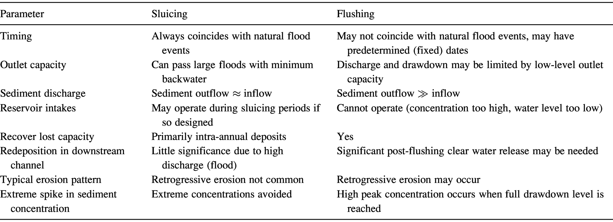
Profile of dam and reservoir operation during a sediment sluicing event, with gate opening timed with flood pulse.

Sluicing is most effective in long and narrow reservoirs that are common to hilly or mountainous terrain. Three Gorges Dam along the middle Yangtze River was engineered to sluice sediment over the long flood season, which usually also results in mobilization of some existing reservoir deposits (Figure 4.49). Three Gorges Reservoir is ideal for sluicing as it is ~600 km long and less than 1.5 km in width (Kondolf et al., Reference Kondolf, Gao and Annandale2014a). While sluicing is considered more environmentally friendly than sediment flushing (Table 4.18), however, aquatic environments downstream of Three Gorges Dam underwent substantial degradation following impoundment, with a near collapse of some fish species (i.e., Figure 4.31). Sediment sluicing is also used on the Sanmenxia Reservoir along the Huanghe (Yellow) River (Wang et al., Reference Wang, Wu and Wang2005), which has long had an enormous sedimentation problem. The concept of sluicing is in accord with the Chinese strategy to release muddy flow and store clear water (Wang and Hu, Reference Wang and Hu2009; Espa et al., Reference Espa, Batalla, Brignoli, Crosa, Gentili and Quadroni2019).
Seasonal pool operation at Three Gorges Dam, Yangtze River, China. Drawdown procedure results in pool lowering by some 30 m during the flood season relative to the normal pool level.

Sediment flushing (or drawdown flushing) is a management approach designed to remove sediment that is already deposited within the reservoir (Morris and Fan, Reference Morris and Fan1998), and must be carefully implemented (Grimardias et al., Reference Grimardias, Guillard and Cattanéo2017; Espa et al., Reference Espa, Batalla, Brignoli, Crosa, Gentili and Quadroni2019). The strategy works by opening low gates near the bottom of the dam structure to lower reservoir levels (Figure 4.50). This increases the hydraulic gradient of the reservoir, and initially scours fine-grained deposits in the lower reservoir, resulting in high suspended sediment concentrations. This is followed by scour of coarser delta deposits higher up in the reservoir that produces bed load transport (Figure 4.50). The timing of reservoir drawdown flushing often occurs during low or moderate flow conditions, rather than during the seasonal flood pulse, which can therefore result in downstream channel bed aggradation. Environmentally, reservoir flushing can be devastating to downstream aquatic habitat, particularly if the channel bed is utilized for critical biological functions – such as fish spawning – and is buried by coarse sandy deposits (Peteuil et al., Reference Peteuil, Fruchart, Abadie, Reynaud, Camenen and Guertault2013). The timing of reservoir drawdown flushing events should be synchronized with crucial ecological functions occurring in the downstream riparian environments, and ideally should occur during the seasonal high-flow period (Wang and Hu, Reference Wang and Hu2009; Kondolf et al., Reference Kondolf, Gao and Annandale2014a; Espa et al., Reference Espa, Batalla, Brignoli, Crosa, Gentili and Quadroni2019).
Profile of dam and reservoir operation during a sediment flushing event. Note drawdown occurs until reservoir is empty, which scours both fine-grained and coarser-grained reservoir deposits. High suspended sediment peaks occur prior to bed material mobilization.


An important consideration within the reservoir concerns the scour and downstream mobilization of polluted reservoir sediments (Evans, Reference Evans2015). The Flix Reservoir along the lower Ebro River in Spain, for example, is only 110 km from Ebro delta wetlands. Unfortunately, adjacent industries historically discharged some 300,000 tons of sediment polluted with mercury (Hg) directly into the reservoir. Improper management of the reservoir flushing regime results in erosion and transport of mercury-polluted sediments from the reservoir to the Ebro Estuary (Palanques et al., Reference Palanques, Guillen, Puig and Grimalt2020).
Finally, along some rivers the main sediment management option is to dredge sediment from reservoirs or other storage sites and transport the sediment downstream by barge, and then dump the sediment into the river for assimilation into the active bed material layer. This approach is utilized along the Rhine Elbe, and Danube Rivers (see Section 8.2.3), for example, to address the sediment starvation problem that has occurred because of numerous dams, hydraulic infrastructure, and land management, which has reduced upstream sediment inputs (Habersack et al., Reference Habersack, Hein and Stanica2016; Frings et al., Reference Frings, Hillebrand, Gehres, Banhold, Schriever and Hoffmann2019).
4.5.2.1 Huanghe River Reservoir Sedimentation: Changing Strategies
Options for managing reservoir sediment need to be adaptable to changing conditions, including climate change and land use change (Wang and Hu, Reference Wang and Hu2009; Graf et al., Reference Graf, Wohl, Sinha and Sabo2011). This can require changes to the dam structure and reservoir management strategies that differ from the original design. Such is the case with the Huanghe River basin. Reservoir sedimentation problems along the Huanghe are well known, and some 21% of the total storage capacity for its seven main-stem reservoirs (i.e., Table 4.8) was lost to reservoir sedimentation by 1989, only about two decades after the first dam was commissioned (Liu et al., Reference Liu, Walling, Spreafico, Ramasmy, Thulstrop and Mishra2017).
Sanmenxia Dam was completed in 1960 (closure) as the first main-stem dam on the Huanghe River (i.e., Table 4.8). The original design was to supply hydropower, irrigation, navigation and downstream flood control, the latter being an epic problem along the lower Huanghe associated with numerous avulsions (see Chapter 7). The initial reservoir management strategy was to store water (Table 4.19). Unfortunately, Sanmenxia was not designed to address the enormous Huanghe sediment loads, the largest sediment loads on Earth, supplied by a legacy of land mismanagement in the upstream Chinese Loess Plateau. Copious sedimentation immediately ensued after dam closure, as only a meagre ~7% of incoming sediment was transported downstream (Table 4.19). A staggering 93% of sediment was stored within the reservoir. Incredibly, by 1965 Sanmenxia reservoir had already lost 41.5% of its reservoir capacity below 335 masl and 62.9% of its storage capacity below 330 masl (Figure 4.51). The sedimentation problems resulted in having the dam redesigned to accommodate sediment sluicing beginning in the early 1970s (Table 4.19), so that the muddy water was released during high-flow events. By the mid-1970s the reservoir had already attained a more consistent storage capacity (Wang et al., Reference Wang, Wu and Wang2005).
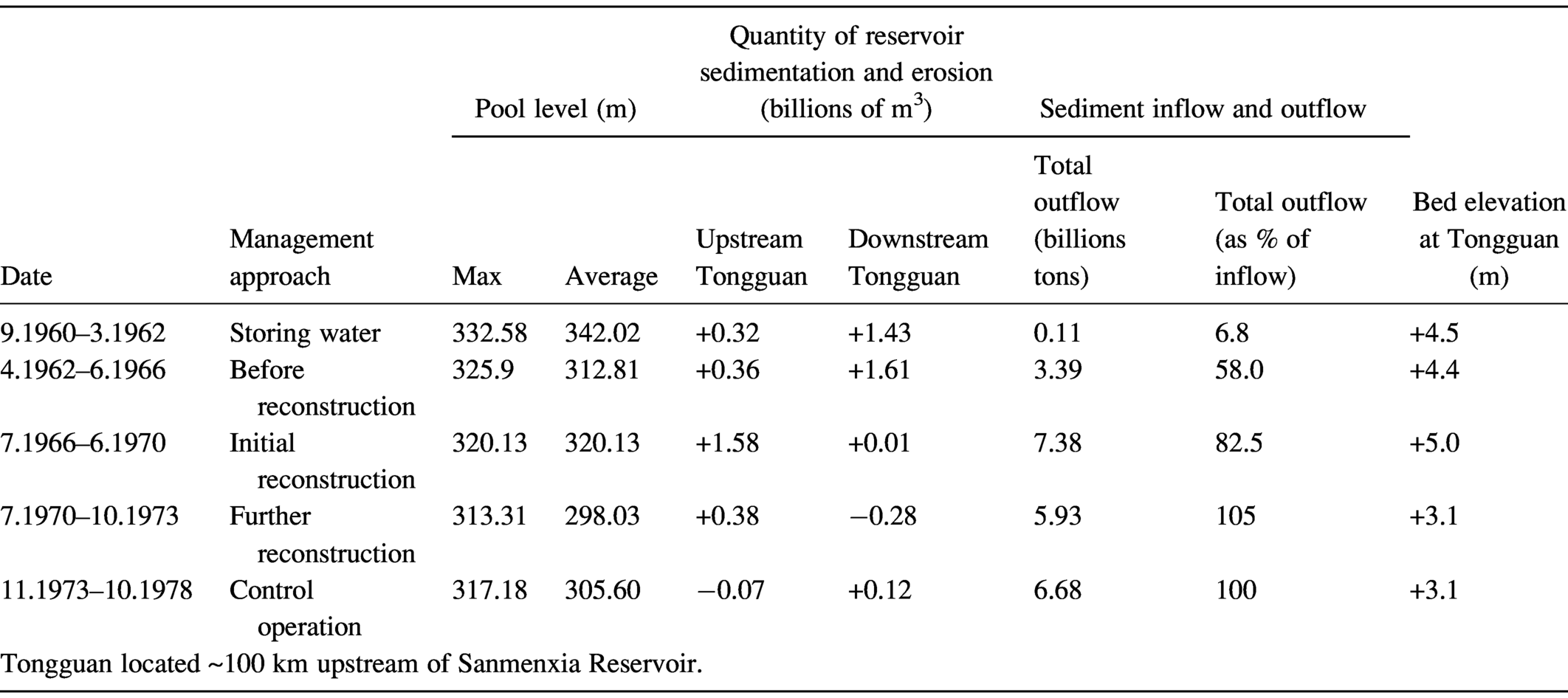
Longitudinal profile of reservoir deposits for Sanmenxia Dam, Huanghe River. Abrupt aggradation occurred soon after closure, and cessation of aggradation after effective reservoir management strategies implemented.

The revised sediment sluicing strategy for Sanmenxia Dam is now part of a larger sediment management approach for the Huanghe basin (Figure 4.52). Since 2002 the Yellow River Conservancy Commission regulates river flow and sediment transport to manage channel bed degradation along a cascade of dams and reservoirs (Liu et al., Reference Liu, Walling, Spreafico, Ramasmy, Thulstrop and Mishra2017; Ma et al., Reference Ma, Nittrouer and Naito2017; Kong et al., Reference Kong, Latrubesse, Miaoa and Zhou2020). The importance of developing an appropriate reservoir sediment management strategy for the Huanghe is as important as any river in the world. Flood disasters along the lower Huanghe River are linked to channel bed aggradation attributed to landscape and sediment mismanagement. The substantial population and economic activities associated with the lower Huanghe riparian environments means that the issue is not only a vital societal concern, but it also influences fluvial dynamics in the lower basin related to channel avulsion, and has implications to the global economy (Section 7.5.2).
Sediment flushing event of Sanmenxia Dam, Huanghe River. Sanmenxia Dam closed in 1960 and is the first main-stem dam on the Huanghe River (contributing drainage area 688,400 km2).

4.5.2.2 Closure: Reservoir Management and Sustaining Rivers
The appropriate sediment management approach for a particular dam and river basin is dependent upon a variety of factors including sediment volume and sediment type (sand/gravel or silt/clay), reservoir geometry (size and shape), streamflow variability, downstream geomorphic and environmental conditions, and expenditures. Adapting the appropriate sediment management strategy can extend the life span of reservoirs beyond the conventional design-life paradigm (Figure 4.53). And, as noted along the Huanghe River, sediment management approaches should be adaptive to accommodate changing boundary conditions and societal priorities because of its impact on the supply of upstream sediment loads (Graf et al., Reference Graf, Wohl, Sinha and Sabo2011; Kondolf et al., 2014a). Identification of an appropriate reservoir sediment management strategy should be seen as a fundamental component of integrated river basin management to support navigation and associated economic activities, mitigate against climate and land use change, and to sustain downstream riparian and linked coastal environments.
Models of dam and reservoir design related to sediment management. Conventional “design-life” paradigm for dams and reservoirs can be modified toward a sustainable use paradigm. New dam construction should include features adaptable to changing sediment management strategies.

It is interesting to ponder a sediment management strategy to Gavins Point Dam (Figure 4.21) on the Missouri River in view of the need to provide sediment to support physical riparian habitat and related biodiversity (NRC, 2011), and the urgent need to supply sediment to construct wetlands in the Mississippi delta (Ahn et al., Reference Ahn, Yang, Boyd, Pridal and Remus2013; Kemp et al., Reference Kemp, Willson, Rogers and Binselam2014). Proposed drawdown flushing strategies designed to scour reservoir deposits and mobilize stored sediment for downstream transport, however, are complicated by the need to consider both the sediment budget of the lower Mississippi as well as specific habitat needs of aquatic species along the lower Missouri, including the endangered Pallid Sturgeon (Scaphirhynchus albus) (Coker et al., Reference Coker, Hotchkiss and Johnson2009; Elliot et al., Reference Elliott, DeLonay, Chojnacki and Jacobson2020; Jacobson et al., Reference Jacobson, Blevins, Bitner, James, Rathburn and Whittecar2009). Nevertheless, identifying a “sustainable” approach to mobilize reservoir sedimentary deposits stored behind Gavins Point Dam, and other Missouri basin dams (Table 4.11), should be of highest priority to responsible government organizations.