1 INTRODUCTION
Stars in the mass range ≈6–12 M⊙ bridge the divide between high-mass stars and low-mass stars, and are characterised by degenerate off-centre carbon ignition prior to a thermally pulsing super asymptotic giant branch (super-AGB) phase. While super-AGB models including the first few thermal pulses have existed for quite some time (e.g. Garcia-Berro & Iben Reference Garcia-Berro and Iben1994; Ritossa, Garcia-Berro, & Iben Reference Ritossa, Garcia-Berro and Iben1996), it is only relatively recently that there has been a resurgence in their study and that full evolutionary models have been computed for the entire thermally pulsing phase (e.g. Siess Reference Siess2010; Ventura & D’Antona Reference Ventura and D’Antona2011; Lau et al. Reference Lau, Gil-Pons, Doherty and Lattanzio2012; Karakas, García-Hernández, & Lugaro Reference Karakas, García-Hernández and Lugaro2012; Gil-Pons et al. Reference Gil-Pons, Doherty, Lau, Campbell, Suda, Guilani, Gutiérrez and Lattanzio2013; Ventura et al. Reference Ventura, Di Criscienzo, Carini and D’Antona2013; Jones et al. Reference Jones2013; Doherty et al. Reference Doherty, Gil-Pons, Siess, Lattanzio and Lau2015). Two major reasons why this class of star had remained relatively understudied for so long are the computational difficulties of following degenerate off-centre carbon ignition and the very large number of thermal pulses expected for super-AGB stars, ranging from tens to even thousands.
One important and highly desirable outcome from stellar calculations for this mass range is a determination of the final fate of such objects. The three critical massesFootnote 1 for intermediate-mass stars, each of which depends on the stellar composition are the following:
-
1. M up, the minimum mass required to ignite carbon;
-
2. M n, the minimum mass for creation of a neutron star via an electron-capture supernova;
-
3. M mas, the minimum mass defining the regime of massive stars, specifically those which undergo all stages of nuclear burning and explode as iron core collapse supernovae (FeCC-SNe).Footnote 2
In the standard picture, a star with a mass below M up will end its life as a CO white dwarf (WD). Stars with masses between M up and M n leave either a CO–Ne or ONe WD remnant, whilst stars with masses between M n and M mas undergo an electron-capture supernova (EC-SN), ending their lives as neutron stars (e.g. Nomoto Reference Nomoto1984; Ritossa, García-Berro, & Iben Reference Ritossa, García-Berro and Iben1999; Siess Reference Siess2007; Poelarends et al. Reference Poelarends, Herwig, Langer and Heger2008; Jones et al. Reference Jones2013; Doherty et al. Reference Doherty, Gil-Pons, Siess, Lattanzio and Lau2015).
A considerable amount of study had been devoted to the explosive deaths of stars in mass range 8–12 M⊙, in particular their potential demise as EC-SNe. The earliest works (e.g. Miyaji et al. Reference Miyaji, Nomoto, Yokoi and Sugimoto1980; Nomoto Reference Nomoto1984; Hillebrandt, Nomoto, & Wolff Reference Hillebrandt, Nomoto and Wolff1984; Nomoto Reference Nomoto1987) involved the evolution of ‘helium balls’ with core masses ~2–2.6 M⊙ through He and C burning with the resultant ONe cores then evolved to conditions very close to the expected explosion. Electron capture SNe are caused by the reduction of pressure support due to electron capture reactions on 24Mg and 20Ne in stars with H-exhausted core masses ~1.375 M⊙ Footnote 3 (Miyaji et al. Reference Miyaji, Nomoto, Yokoi and Sugimoto1980; Hillebrandt et al. Reference Hillebrandt, Nomoto and Wolff1984; Nomoto Reference Nomoto1987). It is electron captures on these isotopes that lead to a reduction both in electron fraction (Y e ) and the Chandrasekhar mass, which triggers contraction (Miyaji et al. Reference Miyaji, Nomoto, Yokoi and Sugimoto1980; Nomoto Reference Nomoto1987). Within this collapsing core, the competition between the energy release by O burning and the reduction in electron pressure due to electron capture reactions determines the fate of the ONe core. The competition between these two processes is sensitive to the density where nuclear burning is ignited, which in turn depends on the adopted input physics (e.g. Isern & Hernanz Reference Isern and Hernanz1994) and initial conditions. In the traditional picture, the density at the time of oxygen ignition is high enough for electron captures to proceed faster than the other nuclear reactions contributing to the nuclear energy production. Oxygen is ignited centrally and the associated deflagration burns the central regions into nuclear statistical equilibrium. The electron capture reactions on this equilibrated material work to further reduce the central density and the subsequent rapid contraction leads to a core collapse. However, if the ignition density is too low, the propagation of the burning front can lead to complete disruption of the core and not to a collapse (see discussions in Nomoto & Kondo Reference Nomoto and Kondo1991; Isern, Canal, & Labay Reference Isern, Canal and Labay1991; Jones et al. Reference Jones, Röpke, Pakmor, Seitenzahl, Ohlmann and Edelmann2016b).
Due to the very steep density gradient in their outer cores, EC-SNe are expected to undergo a prompt explosion, which results in less time for asymmetries to develop; hence, they are expected to receive only a small natal kick (Podsiadlowski et al. Reference Podsiadlowski, Langer, Poelarends, Rappaport, Heger and Pfahl2004; van den Heuvel Reference van den Heuvel, di Salvo, Israel, Piersant, Burderi, Matt, Tornambe and Menna2007; Wanajo, Janka, & Müller Reference Wanajo, Janka and Müller2011), have a low explosion energy (Kitaura, Janka, & Hillebrandt Reference Kitaura, Janka and Hillebrandt2006; Janka et al. Reference Janka, Müller, Kitaura and Buras2008) and show low 56Ni production (Kitaura et al. Reference Kitaura, Janka and Hillebrandt2006; Wanajo et al. Reference Wanajo, Müller, Janka and Heger2017).
The study of Ritossa et al. (Reference Ritossa, García-Berro and Iben1999) was the first to follow the stellar structure of a thermally pulsing super-AGB star, including the stellar envelope, to conditions close to collapse. In recent years, a new generation of progenitor models of EC-SNe has been computed that now evolve super-AGB stars to conditions of collapse (Takahashi et al. Reference Takahashi, Yoshida and Umeda2013) including along the entire thermally pulsing super-AGB phase (Jones et al. Reference Jones2013).
Determining the mass boundary between stars that do and do not explode as supernovae is a topic of vital importance in astrophysics, for many reasons. For example, the supernova rate in part determines the number of neutron stars and the total energy released by supernovae into the environment. Based on a standard initial mass function (IMF), there are as many stars born with masses between 5 and 10 M⊙ as there are with masses greater than 10 M⊙, so how these elusive stars live and die is of interest to many subfields of astrophysics. This mass boundary is also important for galactic chemical evolution and dust evolution models because stars on either side of this divide have significantly different chemical and dust production properties. Due to the shape of the IMF, super-AGB stars are both the rarest of the low/intermediate mass stars, and also the most common of the stars on the more massive side of the boundary. Hence, if they do indeed produce EC-SNe, then they may make a significant contribution to the overall SN rate.
Until recently there have been a few chemical yields available for these stars. Chemical evolution calculations had to use some strategy to deal with missing yields for this mass range. The two most common strategies were to either totally ignore the yields for this mass range or interpolate in mass between yields for the low and high-mass stars. Either is likely to introduce significant errors.
The evolution of massive AGB stars (at the low-mass end) and massive stars (at the high-mass end) is quite different and the evolution between these is qualitatively different to both, so interpolation is very unlikely to be accurate. Because reliable yields have been missing, super-AGB stars have long been suspected to contribute to solving various astrophysical problems, such as the origin of the multiple populations in globular clusters. We return to this question later.
Super-AGB stars are very difficult to identify observationally, with no confirmed detections extant. There is only one strong candidate, the very long period (1 749 days) and high luminosity (M bol ≃ −8.0) star MSX SMC 055 (Groenewegen et al. Reference Groenewegen, Sloan, Soszyński and Petersen2009). Another hindrance to identifying super-AGB stars is that their high luminosities and very large, cool, red stellar envelopes make them almost indistinguishable from their slightly more massive red super-giant counterparts. Indirect evidence for super-AGB stars comes from observations of massive O-rich white dwarfs (Gänsicke et al. Reference Gänsicke, Koester, Girven, Marsh and Steeghs2010), and also from neon novae (Jose & Hernanz Reference Jose and Hernanz1998; Wanajo, Hashimoto, & Nomoto Reference Wanajo, Hashimoto and Nomoto1999; Downen et al. Reference Downen, Iliadis, José and Starrfield2013), with the neon from which their name derives assumed to have been dredged-up from the interior of ONe WDs, the remains of an earlier super-AGB phase.
In Section 2, we discuss the main evolution characteristics of intermediate-mass stars including the thermally pulsing super-AGB phase. In Section 3, we examine the mass limits defining the various evolutionary channels, in particular the final fates of super-AGB stars, including the importance of the binary star channel for formation of EC-SNe. In Section 4, we describe the nucleosynthesis and stellar yields from super-AGB stars. We apply these yields to the globular cluster abundance anomaly problems and examine their relative galactic contribution, and briefly touch upon dust production by super-AGB stars. Last, in Section 5, we discuss the observational studies, reiterate the most critical uncertainties and discuss future directions in super-AGB star research. In this review, we do not consider super-AGB stars in the early universe. For a review on the evolution of primordial and extremely metal-poor super-AGB stars, we refer to the companion paper by Gil-Pons et al. (2017) in this edition.
2 EVOLUTION
2.1. Phases prior to carbon burning
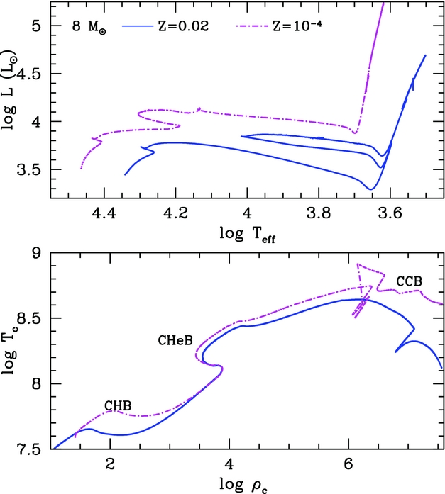
The main nuclear burning stages of intermediate-mass stars are well known, with the stars undergoing convective core H-burning (CHB) via the CNO cycles followed by convective core He-burning (CHeB). In Figure 1, we show the Hertzsprung–Russell diagram for two 8 M⊙ models of metallicities Z = 0.02 and 10−4 through to the super-AGB phase. Clearly seen in this figure is the impact of metallicity on the evolution, with the lower metallicity object being both more luminous and hotter for the same initial mass. At decreasing metallicity, stars attain higher central temperatures to counteract fewer CNO seeds (and associated energy generation). These factors result in a larger core mass for the same initial mass. Due to the earlier ignition of CHeB in the lower metallicity model, the (first) giant branch is avoided and the star does not undergo a first dredge-up event (Girardi et al. Reference Girardi, Bressan, Chiosi, Bertelli and Nasi1996). Figure 1 also shows the evolution of central temperature T c versus central density ρc for the models previously described. We clearly see the occurrence of central H burning at higher temperatures for the lower metallicity model. Once central H is exhausted, the evolution of the stars in the T c–ρc diagram becomes very similar because of the strong dependence of the nuclear burning rates on temperature.
Evolution in the Hertzsprung–Russell diagram (top panel) and in the log central density versus log central temperature diagram (bottom panel) of the 8 M⊙ models of super-AGB stars of metallicities Z = 0.02 and 10−4 from Doherty et al. (Reference Doherty, Gil-Pons, Siess, Lattanzio and Lau2015). CHB, CHeB, and CCB refer to central H, He, and C burning, respectively.
During CHeB, the core is converted to 12C and 16O via the triple-α and 12C(α, γ)16O reactions with the 14N produced from previous CNO cycling being converted to 22Ne via the reaction chain 14N(α, γ)18F(β+ν)18O(α, γ)22Ne. The central 12C content varies strongly with the core mass, with more massive cores having less residual carbon due to higher internal temperatures (Siess Reference Siess2007). Typically, intermediate mass stars have carbon mass fractions of ~0.2–0.5 at the end of CHeB, with this value highly dependent on the 12C(α, γ)16O reaction rate and treatment of mixing (Imbriani et al. Reference Imbriani, Limongi, Gialanella, Terrasi, Straniero and Chieffi2001; Straniero et al. Reference Straniero, Domínguez, Imbriani and Piersanti2003).
The duration of the CHB and CHeB phases varies with metallicity and a variety of other factors such as treatment of convective boundaries, semiconvection, rotation,Footnote 4 and nuclear reaction rates, particularly the rate of the 12C(α, γ)16O reaction during the later phases of CHeB. Typically, the main sequence lifetime of intermediate mass stars in the mass range considered here (≈6–12 M⊙) is between about 18–60 Myr with the CHeB phase being considerably shorter, of the order 2–5 Myr.
For the same initial mass, intermediate-mass stars of lower metallicity will have a shorter lifetime albeit only slightly, with the 8 M⊙ models presented here showing a difference in main sequence lifetime of only ~10%.
2.2. Carbon burning phase
Here, we provide an overview of the carbon burning phase within super-AGB stars, whilst very detailed descriptions of this phase can be found in works such as Garcia-Berro & Iben (Reference Garcia-Berro and Iben1994), Siess (Reference Siess2006) and Farmer, Fields, & Timmes (Reference Farmer, Fields and Timmes2015).
Once CHeB has ceased, the resulting CO core begins to contract. The time from the cessation of CHeB to C ignition is a function of core mass with larger core masses evolving more rapidly, and typical values of 1.5–3 × 10⁵ yr (Doherty et al. Reference Doherty, Siess, Lattanzio and Gil-Pons2010). This contraction causes an increase in the central density, which leads to neutrino energy losses becoming important for the innermost regions of the star. This results in cooling and the formation of a temperature inversion. When the peak temperature reaches approximately 640 × 106 K, and the density at that point is about 1.6 × 10⁶ g cm−3, carbon is ignited. This ignition takes place off-centre and under conditions of partial degeneracy with η ~ 2–3, where η is the degeneracy parameter. The peak carbon burning luminosity during this initial violent carbon burning flash can be up to about 109 L⊙ and the large energy release drives the formation of a convective zone. After a short period, this first carbon flash is quenched and contraction of the core resumes, to be followed by another carbon flash. In this second flash, the degeneracy is lower (η ~ 1) and the convective region that forms (classified as a ‘flame”) subsequently burns inwards until it reaches the centre. Carbon burning however is not complete and continues radiatively outwards, generating secondary convective flashes when regions of high carbon content are encountered. The specific number of flashes depends on the degeneracy of the core, and thus on the star’s initial mass. In general, lower-mass objects tend to experience a higher number of secondary flashes and with higher intensity.
The effect of the carbon-burning flashes and flame on the central region can be seen in the bottom panel of Figure 1. For the Z = 10−4 model, the initial flash causes a sharp drop in both temperature and density (down to log T~8.5 and log ρ ~ 6). The point at which the flame reaches the centre is quite evident, being characterised by the large and steep rise in the central temperature at about constant density (log ρ ~ 6)Footnote 5 . The strength of the initial carbon flash is larger in the more degenerate (i.e. less massive) models, with the carbon flash luminosities ranging from ~106 to 109 L⊙. The more massive models also ignite carbon closer to the centre, under conditions of milder degeneracy than is the case for lower mass stars.
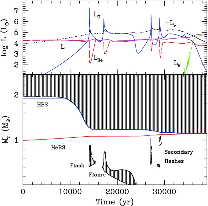
Figure 2 is a Kippenhahn diagram of an 8.5 M⊙ Z = 0.02 model and illustrates the typical multi-step burning process, consisting of an off-centre flash, a flame that propagates towards the centre, and then subsequent secondary carbon flashes in the outer parts of the core. In the top panel, the evolution of H, He, C, neutrino and total luminosities is shown. Clearly seen are the carbon burning flashes/flame with peaks in L C. The total luminosity of the star is almost constant through the carbon burning phase with its behaviour decoupled from the central burning regions. During the steady carbon burning flame phase, all of the energy released by carbon burning is carried away by neutrinos, in what is called the ‘balanced power condition’ (Timmes, Woosley, & Taam Reference Timmes, Woosley and Taam1994), as can be seen in Figure 2. The carbon burning flame speed is quite slow ~10−2–10−3 cm s−1 (Timmes et al. Reference Timmes, Woosley and Taam1994; Ritossa et al. Reference Ritossa, Garcia-Berro and Iben1996; Siess Reference Siess2006). The duration of the carbon burning phase decreases with increasing core mass (i.e. initial mass) and ranges between about 10 000 and 40 000 years. The minimum CO core masses for C-burning is ~1.05 M⊙.
Kippenhahn and luminosity diagram during the carbon burning phase for an 8.5 M⊙ model with Z = 0.02 from Doherty et al. (Reference Doherty, Gil-Pons, Siess, Lattanzio and Lau2015). Time has been set to zero when L C first exceeds 1 L⊙. In the upper panel, we show different luminosity sources: H in green, He in dashed red, C in blue, surface in magenta, and the negative of the neutrino luminosity is in black. In the lower panel, the mass coordinate of the HBS is shown in blue, the HeBS in red, and the hatched regions represent convection.
The main nuclear reactions during the carbon burning phase are 12C(12C,p)23Na and 12C(12C,α)20Ne, followed by 23Na(p,α)20Ne and 16O(α, γ)20Ne. The carbon burning rates are quite uncertain, and it has been suggested that there may be unmeasured resonances (Spillane et al. Reference Spillane2007; Cooper, Steiner, & Brown Reference Cooper, Steiner and Brown2009) or hindrances (Jiang et al. Reference Jiang, Rehm, Back and Janssens2007), which may alter the rates by more than a factor of 1 000 compared to the standard rates from Caughlan & Fowler (Reference Caughlan and Fowler1988). Due to their importance for a variety of stellar environments, in particular in Type 1a SN studies, these reaction rates are currently under much investigation (e.g. Bucher et al. Reference Bucher2015). Chen et al. (Reference Chen, Herwig, Denissenkov and Paxton2014) examined the impact of variations to the 12C + 12C rates on carbon burning within super-AGB stars and found that if the rates were multiplied by factors of 1 000 and 0.01, the minimum CO core mass for carbon ignition became 0.93 M⊙ and 1.10 M⊙, respectively.
After the completion of core carbon burning (CCB), the core has been converted to mostly 16O (50–70%), 20Ne (15–35%) and trace amounts of 23Na, 24, 25, 26Mg, 21, 22Ne and 27Al (Siess Reference Siess2007). The third most common element in the cores varies between calculations and is either Mg (Nomoto Reference Nomoto1984; Miyaji et al. Reference Miyaji, Nomoto, Yokoi and Sugimoto1980; Takahashi et al. Reference Takahashi, Yoshida and Umeda2013) or Na (Garcia-Berro & Iben Reference Garcia-Berro and Iben1994; Siess Reference Siess2006), which results in either ONeMg or ONeNa cores. The amount of Mg or Na may have important implications in the subsequent evolution if the stellar core grows to conditions for an EC-SN e.g. Gutiérrez, Canal, & García-Berro (Reference Gutiérrez, Canal and García-Berro2005). There is also a small abundance of 12C remaining throughout the ONe core of about 0.2–2%, with this residual carbon abundance being lower in the more massive models.
In the traditional picture, stars with ONe core masses exceeding 1.37 M⊙ Footnote 6 at the end of C-burning will ignite neon and undergo all stages of further burning (Nomoto Reference Nomoto1984). Therefore, ONe cores are expected to be produced with masses ~1.06–1.37 M⊙.
2.2.1. An important aside on convective borders
It is well known that convective flows may lead to mixing beyond the formal Schwarzschild boundary, which is the position where the buoyancy force is zero. This is often referred to as ‘convective overshoot’. Historically, this term was used for the case where momentum carried a hypothetical fluid element beyond the Schwarzschild border (where the acceleration is zero). The true border is where the velocity reaches zero.
There are two common approaches to modelling this overshoot. In the simplest case, one simply extends the convective region by a chosen amount, typically a multiple αover times the local pressure scale-height H p. Another approach is due to Herwig et al. (Reference Herwig, Bloecker, Schoenberner and El Eid1997), which is based on the study of Freytag, Ludwig, & Steffen (Reference Freytag, Ludwig and Steffen1996). Here, one introduces a diffusion coefficient D OV, which is used beyond the formal convective border. Herwig et al. (Reference Herwig, Bloecker, Schoenberner and El Eid1997) proposed
 $$\begin{equation}
D_{\rm OV} = D_{0} \text{exp} {\left(\frac{-2z}{f_{\rm {over}} H_{\rm p}}\right),}
\end{equation}$$
$$\begin{equation}
D_{\rm OV} = D_{0} \text{exp} {\left(\frac{-2z}{f_{\rm {over}} H_{\rm p}}\right),}
\end{equation}$$
where D 0 is the diffusion coefficient near the convective boundary, z is the radial distance from the edge of the convective zone and H p is the pressure scale height at the convective edge.
Typically, the amount of overshooting used in stellar calculations is based on calibrations to a variety of observations such as the width of the main sequence in stellar clusters, eclipsing binaries (e.g. Schaller et al. Reference Schaller, Schaerer, Meynet and Maeder1992; Schroder, Pols, & Eggleton Reference Schroder, Pols and Eggleton1997; Claret Reference Claret2007; Stancliffe et al. Reference Stancliffe, Fossati, Passy and Schneider2015) and more recently on asteroseismic observations (e.g. Montalbán et al. Reference Montalbán, Miglio, Noels, Dupret, Scuflaire and Ventura2013; Aerts Reference Aerts, Pavlovski, Tkachenko and Torres2013). In the case of the exponential diffusive approach, the value of f over = 0.016 was shown to reproduce the observed width of the main sequence (Herwig Reference Herwig2000). We note that αover ≈ 10 × f over (Herwig et al. Reference Herwig, Bloecker, Schoenberner and El Eid1997; Stancliffe et al. Reference Stancliffe, Fossati, Passy and Schneider2015), with αover values from the literature typically in the range 0.1–0.4 (e.g. Schaller et al. Reference Schaller, Schaerer, Meynet and Maeder1992; Stancliffe et al. Reference Stancliffe, Fossati, Passy and Schneider2015; Claret & Torres Reference Claret and Torres2016).
However, we note that it is possible, even likely, that other mechanisms may be involved, such as gravity waves, or other hydrodynamical phenomena. In lieu of a complete theory to describe the behaviour of the fluid at the convective boundary, we shall instead refer to ‘convective boundary mixing’ (hereinafter CBM) as the generic process(es) acting at this location. CBM is usually specified via some numerical algorithm, which must suffice until we have a better description of the behaviour of the fluid at convective boundaries.
2.2.2. Incomplete C-burning—hybrid CO–Ne cores
In stars with initial mass slightly above M up, carbon ignites in the very outer regions of the core. In some cases, after the primary flash has occurred, no further carbon burning takes place. These aborted carbon ignition models have an interior comprised of a very large central CO region surrounded by a thin ONe layer and a further outer CO region (e.g. Doherty et al. Reference Doherty, Siess, Lattanzio and Gil-Pons2010; Ventura & D’Antona Reference Ventura and D’Antona2011). The initial mass range for creation of this class of hybrid CO–Ne cores is very narrow, being at most about 0.1 M⊙. CO–Ne cores can also be formed when the carbon burning flame stalls on its journey towards the centre.
Due to off-centre (convective) carbon burning in super-AGB stars, a molecular weight inversion is created, which can drive thermohaline mixing (Siess Reference Siess2009). The resultant mixing transports carbon from the inner region towards the burning flame, replacing it with the heavier products of carbon burning. Thermohaline mixing below the C-convective shell is thus able to decrease significantly the C content in the zones ahead of the C-burning flame, and deprived of fuel, this causes the extinction of the flame before it reaches the centre. The result is a hybrid degenerate core, comprising an inner zone of unburnt (but depleted) CO and an outer ONe zone. In such a case, in contrast to calculations that do not include thermohaline mixing, the ONe core is left with a larger amount of unburnt 12C, between 2% and 5%, in the centre.
Later, using downward revised values of the thermohaline mixing coefficient based on multi-dimensional hydrodynamic simulations, Denissenkov et al. (Reference Denissenkov, Herwig, Truran and Paxton2013) discounted the ability of thermohaline mixing to stall the carbon burning flame, suggesting that the mechanism was too inefficient. Some CBM was included by Denissenkov et al. (Reference Denissenkov, Herwig, Truran and Paxton2013) at the base of the C-burning convective shell of super-AGB stars, where the C-burning flame was indeed deprived of fuel and stalled. This resulted in hybrid CO–Ne cores being formed.
For determining the composition of stellar material, the main difference between thermohaline mixing and CBM concerns the extent of the induced mixing. Thermohaline mixing connects the entire interior to the region with the higher molecular weight that is being produced by the burning flame. With CBM, the mixing only occurs directly below the convection over a region whose width is determined by some model or algorithm. In contrast to thermohaline mixing, this leaves a pristine CO core interior to the maximum extent of the CBM. Thus, CBM also produces hybrid CO–Ne cores, but these hybrids can be produced with a range of configurations and quite widely varying widths of the ONe shell. This is unlike the structures produced from the lower-mass super-AGB stars that have thin ONe shells in the far outer core.
Chen et al. (Reference Chen, Herwig, Denissenkov and Paxton2014) investigated the effects of CBM and the quite uncertain 12C reaction rates on hybrid core creation. They found that varying the efficiency of CBM in addition to the 12C reaction rates resulted in the formation of hybrid CO–Ne cores over a wide range of core masses from ≈0.93–1.30 M⊙. This corresponds to an initial mass range for hybrid CO–Ne core creation (defined as $\Delta M_{\rm {CO\text{--}Ne}}$
) of up to 1 M⊙, which would make the CO–Ne cores very common. This wide channel and very large core mass of 1.30 M⊙ for hybrid CO–Ne WDs could have important implications for the rate of Type 1a SNe due to an increased initial-mass range for progenitors, a reduction of core growth required prior to explosion, and to a reduced delay time between star formation bursts and the occurrence of Type 1a SNe (e.g. Meng & Podsiadlowski Reference Meng and Podsiadlowski2014; Wang et al. Reference Wang, Meng, Liu, Liu and Han2014; Liu et al. Reference Liu, Stancliffe, Abate and Wang2015; Denissenkov et al. Reference Denissenkov, Herwig, Truran and Paxton2013).
$\Delta M_{\rm {CO\text{--}Ne}}$
) of up to 1 M⊙, which would make the CO–Ne cores very common. This wide channel and very large core mass of 1.30 M⊙ for hybrid CO–Ne WDs could have important implications for the rate of Type 1a SNe due to an increased initial-mass range for progenitors, a reduction of core growth required prior to explosion, and to a reduced delay time between star formation bursts and the occurrence of Type 1a SNe (e.g. Meng & Podsiadlowski Reference Meng and Podsiadlowski2014; Wang et al. Reference Wang, Meng, Liu, Liu and Han2014; Liu et al. Reference Liu, Stancliffe, Abate and Wang2015; Denissenkov et al. Reference Denissenkov, Herwig, Truran and Paxton2013).
Farmer et al. (Reference Farmer, Fields and Timmes2015) studied carbon ignition within intermediate/massive stars with an extensive grid of models looking at the effects of rotation, convective overshooting (using the formalism of Herwig et al. (Reference Herwig, Bloecker, Schoenberner and El Eid1997) with f over in the range 0–0.02), thermohaline mixing and combinations of these processes. In their study, they found that a substantial number of stars which ignited carbon off-centre went on to form CO–Ne cores. In particular, in agreement with Denissenkov et al. (Reference Denissenkov, Herwig, Truran and Paxton2013) and Chen et al. (Reference Chen, Herwig, Denissenkov and Paxton2014), models with efficient overshooting at the base of the convective carbon burning region led to a very wide initial-mass range for hybrid CO–Ne WDs.
Recently, a work by Lecoanet et al. (Reference Lecoanet2016) using 3D hydrodynamic simulations has suggested that convective mixing cannot stall the carbon burning flame due to the large buoyancy barrier that needs to be crossed to reach the radiative burning front, and hence formation of CO–Ne WDs would not be typical. Irrespective of whether CO–Ne cores could actually form, Brooks et al. (Reference Brooks, Schwab, Bildsten, Quataert and Paxton2017) showed that a structure composed of a higher density ONe mantle above a CO core would be unstable to rapid mixing shortly after the onset of the WD cooling sequence. Thus, the actual occurrence of hybrid cores and their possibility to remain unmixed throughout the latest stages of stellar lives is still a matter of debate.
One of the main interests in hybrid cores is related to the potential eventual fates of SNIa. The amount of available C would probably be high enough so that, if the degenerate core were able to increase in mass up to M Ch, a thermonuclear (single) SN explosion would result (Poelarends et al. Reference Poelarends, Herwig, Langer and Heger2008). Alternatively, if the super-AGB star were the primary component of a close binary system with specific initial orbital parameters, SNIa explosions might occur.
This possibility was explored by Bravo et al. (Reference Bravo, Gil-Pons, Gutiérrez and Doherty2016), who computed the hydrodynamical explosion of white dwarfs hosting hybrid cores, under different conditions (size of the hybrid cores, and ignition by deflagration or detonation). These authors showed that SNIa harbouring hybrid cores would be characterised by lower kinetic energies and lower amounts of ejected 56Ni than their pure CO WD counterparts. Explosions of these hybrid cores may be the theoretical counterparts of the sub-luminous class of SN2002 cx-like SN or SNIax. Denissenkov et al. (Reference Denissenkov, Truran, Herwig, Jones, Paxton, Nomoto, Suzuki and Toki2015) also pointed out the fact that hybrid CO–Ne cores might be one possible reason for the inhomogeneity of observed SNIa. The multi-dimensional hydrodynamical simulations by Kromer et al. (Reference Kromer2015) and Willcox et al. (Reference Willcox, Townsley, Calder, Denissenkov and Herwig2016) also reproduced the same trend, that is, their SNIa models hosting hybrid degenerate cores also produce less 56Ni and release less kinetic energy.
2.2.3. Incomplete Ne-burning – failed massive stars
The ability of the Ne burning flame to propagate to the centre is of crucial importance in determining if the star ends its life as an EC-SN or an FeCC-SN. As mentioned in Section 2.2, if the ONe core mass exceeds 1.37 M⊙, it is assumed that Ne shall ignite and the star will follow the massive star channel. However, there are slight complications to this standard picture. The behaviour of Ne burning is very similar to that seen during the earlier phase of C burning. Efficient neutrino cooling causes the temperature maximum to move away from the centre, resulting in Ne ignition occurring further off-centre for lower masses. Akin to the aborted carbon ignition models described in Section 2.2.2, if neon is ignited at the very outer edge of the core, there will be a brief neon flash but neither subsequent burning nor flame propagation (Timmes et al. Reference Timmes, Woosley and Taam1994; Ritossa et al. Reference Ritossa, García-Berro and Iben1999; Eldridge & Tout Reference Eldridge and Tout2004). It is expected that these stars with core masses so close to the Chandrasekhar mass will end life as EC-SNe after a very brief thermally pulsing phase. Doherty et al. (Reference Doherty, Gil-Pons, Siess, Lattanzio and Lau2015) proposed a new nomenclature for models that undergo only very slight off-centre neon burning and then later reach the thermally pulsing super-AGB phase, calling them ‘hyper-AGB’ stars.
In addition to the super-AGB evolution towards an EC-SN, a second possible single star EC-SN channel exists, that of ‘failed massive stars’ (Jones et al. Reference Jones2013; Jones, Hirschi, & Nomoto Reference Jones, Hirschi and Nomoto2014). A failed massive star is formed in stars with ONe core masses slightly above the value for Ne ignition. If Ne is ignited far enough off-centre and convective boundary mixing is employed at the base of the Ne burning shell, then instead of a flame progressing smoothly towards the centre, the Ne burning can be stalled and undergo multiple flashes. After each flash, there is a period of contraction that, given enough time, can ultimately result in the core reaching sufficient densities for the Urca processes to be activated and the star to subsequently reach conditions for an EC-SN prior to the Ne flame being able to reach the centre. However, if no CBM is employed and the strict Schwarzschild boundary is used at the base of the Ne convective region, as can be seen in Jones et al. (Reference Jones, Hirschi and Nomoto2014), then the class of failed massive stars ceases to exist and the Ne flame is free to propagate inward towards the centre with the star most likely becoming an FeCC-SN. The exact contribution from failed massive stars to the EC-SN channel is highly uncertain, but if this class of star only occurs for models in which the H-exhausted core has been reduced to precisely the Chandrasekhar mass, (refer to next Section 2.3), then we expect a narrow channel.
2.3. Reduction of H-exhausted core mass
For intermediate-mass stars, the H-exhausted core masses after CHe burning are in the range ≈1.6–2.6 M⊙. Hence, after CHeB all future super-AGB stars will eventually grow degenerate core masses far exceeding the Chandrasekhar mass (M Ch) and therefore if no process takes place to reduce the core mass, these stars will undergo all stages of core burning, just as do massive stars.
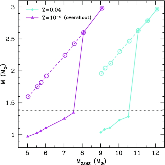
Prior to the thermally pulsing phase, two processes can reduce this H-exhausted core mass, these being second dredge-up (hereafter SDU) and dredge-out. Figure 3 shows the H-exhausted core mass both before and after SDU. Clearly seen is the sharp divide between stars that undergo SDU and those that do not. This figure also highlights that this same behaviour occurs over a large spread in metallicity, and both with and without convective overshooting.
Mass of the H-exhausted core before (open circles connected by a dashed line) and after (triangles/diamonds connected by a solid line) the operation of the SDU for two metallicities. The left/magenta and right/cyan lines correspond to models with a metallicity Z = 10−4 (with core overshooting) and Z = 0.04 (without core overshooting), respectively. The dotted horizontal line represents the Chandrasekhar mass. Models are from Siess (Reference Siess2007) with overshoot as described in Herwig et al. (Reference Herwig, Bloecker, Schoenberner and El Eid1997) with a value f over = 0.016.
2.3.1. Second dredge-up
Due to the gravitational contraction of the core after CHeB, the envelope expands and cools, with convection penetrating inwards into the H exhausted core (Becker & Iben Reference Becker and Iben1979). The SDU event occurs at different stages of the C-burning phase for stars of different initial masses. For low-mass super-AGB stars, it takes place prior the first C-flash. Stars of higher initial mass evolve faster and thus ignite C earlier. Normally, SDU only brings to the surface material that has undergone H burning. However, the more massive stars can experience what is called a ‘corrosive” SDU episode (Gil-Pons et al. Reference Gil-Pons, Doherty, Lau, Campbell, Suda, Guilani, Gutiérrez and Lattanzio2013; Doherty et al. Reference Doherty, Gil-Pons, Lau, Lattanzio, Siess and Campbell2014b): in these cases the bottom of the convective envelope is able not only to reach below the former HBS, but also to reach deeper, to where the products of the HeBS reside. Corrosive SDU enriches the surface with substantial amounts of primarily 12C (and 18O, e.g. Becker & Iben Reference Becker and Iben1979; Herwig Reference Herwig2004), while in the more massive models corrosive SDU also enriches the surface with substantial amounts of 16O. The masses of the stellar cores for which corrosive SDU occurs vary between studies, with about 1.15–1.28 M⊙ in Doherty et al. (Reference Doherty, Gil-Pons, Lau, Lattanzio, Siess and Campbell2014b), down to 1.03 M⊙ in Herwig (Reference Herwig2004). These values are generally lower for lower metallicity models due to their broader residual He shells. The degree of metal enrichment from SDU in the envelope of low metallicity stars is critical for their future evolution.
2.3.2. The dredge-out episode
Ritossa et al. (Reference Ritossa, García-Berro and Iben1999) first named, described and provided an extensive analysis of the phenomenon known as dredge-out. It was later reported by Siess (Reference Siess2007), Poelarends et al. (Reference Poelarends, Herwig, Langer and Heger2008), Takahashi et al. (Reference Takahashi, Yoshida and Umeda2013), Gil-Pons et al. (Reference Gil-Pons, Doherty, Lau, Campbell, Suda, Guilani, Gutiérrez and Lattanzio2013), Doherty et al. (Reference Doherty, Gil-Pons, Siess, Lattanzio and Lau2015) and Jones et al. (Reference Jones, Ritter, Herwig, Fryer, Pignatari, Bertolli and Paxton2016a) using different evolutionary codes and different input physics (in particular the treatment of mixing and treatment of convective borders). This phenomenon occurs for massive super-AGB stars regardless of their metallicity (e.g. Gil-Pons et al. Reference Gil-Pons, Doherty, Lau, Campbell, Suda, Guilani, Gutiérrez and Lattanzio2013) and occurs for stars in the upper ≈ 0.3 M⊙ range of super-AGB stars.
Figure 4 shows the evolution during C-burning and dredge-out phase for a 9.5 M⊙ Z = 0.001 star from Siess (Reference Siess2007). Nearing the end of the carbon burning phase, a convective He shell develops near the upper boundary of the partially degenerate core. This shell is initially separated from the base of the convective envelope by a relatively extended radiative region (about 1 M⊙) and a thin semiconvective region near the He–H interface. As described in Ritossa et al. (Reference Ritossa, García-Berro and Iben1999), the He convective shell is initially sustained mainly by C-burning, and gravothermal energy, but He-burning powers its final approach towards the base of the convective envelope. Eventually, these convective regions meet and protons are ingested into very high temperature (≳ 108 K) He- and C-rich regions. These ingested protons rapidly undergo the 12C(p,γ)13N reaction leading to a H-flash with peak luminosities of L H ~ 109 L⊙. The associated total energy release from the H-flash is vast, and is generated in a very small region. According to estimates by Jones et al. (Reference Jones, Ritter, Herwig, Fryer, Pignatari, Bertolli and Paxton2016a), the energy released by this process represents about 11% of the internal energy and about 8% of the binding energy of the combustive flame layer. It is likely that this has hydrodynamical consequences and the assumption of hydrostatic equilibrium should be doubted. At the very least, it is likely that time-dependent convection is required (Herwig et al. Reference Herwig, Pignatari, Woodward, Porter, Rockefeller, Fryer, Bennett and Hirschi2011). Jones et al. (Reference Jones, Ritter, Herwig, Fryer, Pignatari, Bertolli and Paxton2016a) suggest that this dredge-out may provoke a phenomena similar to the global oscillation of shell-H ingestion (GOSH) event (Herwig et al. Reference Herwig, Woodward, Lin, Knox and Fryer2014), which could potentially drive more powerful and non-radial hydrodynamic events leading to mass ejection.
Kippenhahn and luminosity diagram during the carbon burning phase and dredge-out episode for a 9.5 M⊙ Z = 0.001 model from Siess (Reference Siess2007). Time is counted backwards from the last computed model.
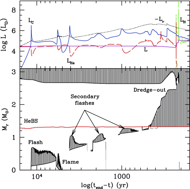
With an abundant supply of 13C now in a high-temperature, helium-rich region, the 13C(α,n)16O reaction is expected to take place at a rapid pace and produce a substantial number of free neutrons (Doherty et al. Reference Doherty, Gil-Pons, Siess, Lattanzio and Lau2015; Jones et al. Reference Jones, Ritter, Herwig, Fryer, Pignatari, Bertolli and Paxton2016a).
A dredge-out event is expected to produce neutron densities of the order N n ≈1015 n cm−3 corresponding to the intermediate n-capture regime (known as the ‘i-process’, see Cowan & Rose Reference Cowan and Rose1977). This process in super-AGB stars was suggested by Jones et al. (Reference Jones, Ritter, Herwig, Fryer, Pignatari, Bertolli and Paxton2016a) to be responsible for the occurrence of some carbon-enhanced metal poor stars enriched in s- and r-process elements (the CEMP s/r stars, see Beers & Christlieb Reference Beers and Christlieb2005). However, based on an IMF argument, the relatively few super-AGB stars seem unlikely to be a major source of pollution of the CEMP s/r stars (Abate, Stancliffe, & Liu Reference Abate, Stancliffe and Liu2016).
Besides the possibility of ejection of heavier-than-iron elements, the dredge-out process also alters surface abundances of light elements, in particular He and the He-burning product 12C (Ritossa et al. Reference Ritossa, García-Berro and Iben1999). This results in the most massive super-AGB stars becoming carbon stars. We discuss the importance of the surface composition during the super-AGB phase in Section 2.4.
In models of slightly lower mass than those that undergo dredge-out, near the end of carbon burning and prior to the SDU, there is also the formation of a convective He region. However, this convective zone decays before the convective envelope penetrates inwards, and therefore does not merge with the proton-rich region. This material will be highly enriched in 12C and will later also be dredged up to the surface (e.g. Herwig et al. Reference Herwig, VandenBerg, Navarro, Ferguson and Paxton2012).
2.4. The thermally pulsing super-AGB phase
After the cessation of core carbon burning a super-AGB star consists of a massive ONe core surrounded by a CO shell, a H-burning shell and a very extended H-rich envelope. Quiescent H-burning is eventually interrupted by unstable He-burning, a thermal pulse ensues and the thermally-pulsing super-AGB (TP-SAGB) phase begins. Early He-flashes tend to be relatively mild, but their peak luminosities grow as the evolution progresses. When the TP-SAGB is established, H-burning and He-burning in shells alternate as nuclear energy suppliers. Figure 5 gives a schematic overview of the typical values from the literature associated with the thermally pulsing phase of super-AGB stars.
Schematic Kippenhahn diagram of two consecutive thermal pulses showing typical values for super-AGB stars. The upper light grey shaded region represents the convective envelope and the two thin shaded regions represent the convective shells associated with two consecutive flashes.
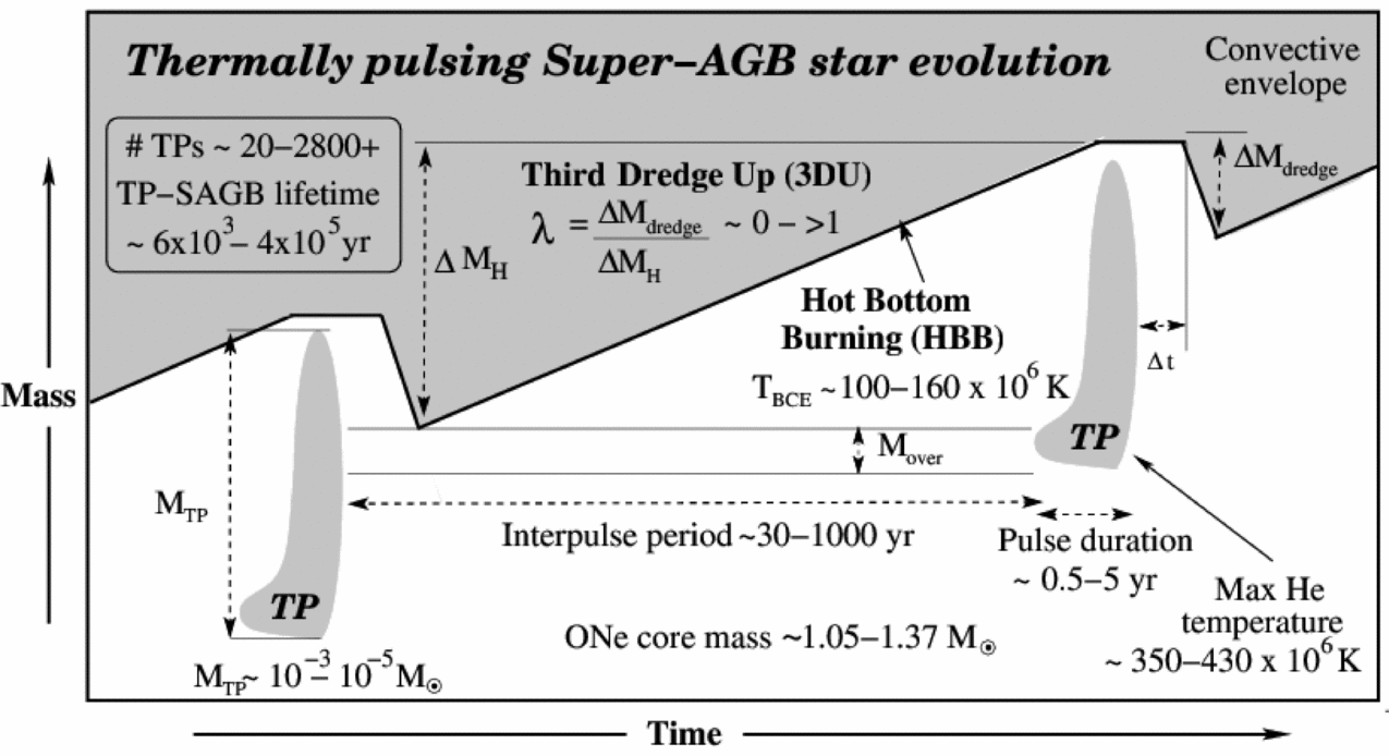
Whilst qualitatively similar to their lower-mass counterparts (for a recent review of AGB stars refer to Karakas & Lattanzio Reference Karakas and Lattanzio2014), super-AGB stars present some important differences. The most obvious is that the stellar cores and envelopes are more massive, between ≈1.06–1.37 M⊙, and ~5–10 M⊙, respectively. Due to their larger, hotter and more compact cores, the recurrence time between thermal pulses (the interpulse period) is much shorter (10s to 1 000s yr) in super-AGB stars and due to this they can undergo from between tens to multiple thousands of thermal pulses, typically with more pulses at lower metallicity. The thermal pulse duration is also greatly reduced in comparison to lower-mass AGB stars, with pulses lasting only about 0.5–5 yr. The intershell convective regions are also thinner, with a mass of only 10−3–10−5 M⊙.
The maximum temperature within the HeB convective zone steadily increases throughout the evolution along the TP-SAGB and also increases with increasing initial mass, with the most massive super-AGB star models achieving temperatures in the range 350–430 × 106 K. This high temperature has important implications for the activation of the 22Ne neutron source and heavy element production (see Section 4.3.2). The strength of the thermal pulses, as measured by the HeB luminosity L He, decreases for super-AGB stars with increasing (initial) core mass. This is due to the reduced temperature sensitivity of the triple α reaction, the higher radiation pressure and the lower degree of degeneracy (e.g. Sackmann Reference Sackmann1977; Sugimoto & Fujimoto Reference Sugimoto and Fujimoto1978; Siess Reference Siess2006). This peak L He value varies widely between computations from different research groups and typically those with less violent thermal pulses have lower dredge-up efficiency. The overlap factor r is defined by r = M over/M TP, where M over is the mass contained in the previous intershell convective zone that is engulfed in the next pulse (see Figure 5) and M TP is the mass of the intershell convective zone at the current thermal pulse. This parameter is important in particular in relation to heavy element production because it determines the amount of material that experiences multiple neutron exposures in subsequent thermal pulses.
Due to the activation of nuclear burning at the base of their convective envelopes, super-AGB stars are more luminous than the classical AGB limit (Paczyński Reference Paczyński1970). The most metal poor models can reach in excess of 105L⊙ (M bol ~ −8.2), which places them at comparable luminosity to the more massive red super-giants.
The third dredge-up (hereafter TDU) is the process where after a thermal pulse the convective envelope penetrates through the (extinct) hydrogen shell and into the intershell region, mixing up products of H and partial He burning. Apart from the enrichment of the envelope composition, another important consequence of the TDU is the reduction in the mass of the H exhausted core. The efficiency of TDU is commonly measured using the λ parameter, defined as ΔM dredge/ΔM H, where ΔM H is the increase in the core mass during the previous interpulse phase and ΔM dredge is the depth of the dredge-up (see Figure 5). By this definition, a λ value of one represents the case where the entire region processed by the H shell during the previous interpulse phase is mixed to the surface during the subsequent TDU episode and there is no overall core growth. We note that there is no physical reason why λ cannot exceed unity.
In super-AGB star modelling, the amount (and even occurrence) of TDU is hotly debated, with computations finding no TDU (e.g. Siess Reference Siess2010; Ventura et al. Reference Ventura, Di Criscienzo, Carini and D’Antona2013), low efficiency TDU with λ ~ 0.07–0.3 (Ritossa et al. Reference Ritossa, Garcia-Berro and Iben1996), moderate efficiency TDU with λ ~ 0.4–0.8 (Doherty et al. Reference Doherty, Gil-Pons, Siess, Lattanzio and Lau2015) and high efficiency TDU with λ > 1 (Herwig et al. Reference Herwig, VandenBerg, Navarro, Ferguson and Paxton2012; Jones et al. Reference Jones, Ritter, Herwig, Fryer, Pignatari, Bertolli and Paxton2016a). Although quantitative differences exist between evolutionary calculations from different research groups, the general trend is for decreasing TDU efficiency (or cessation of TDU entirely) as one transitions from intermediate/massive AGB stars, meaning those with initial masses ≳ 5 M⊙ but not massive enough to ignite carbon, to super-AGB stars, which do ignite carbon.
Jones et al. (Reference Jones, Ritter, Herwig, Fryer, Pignatari, Bertolli and Paxton2016a) examined the variations to the efficiency of TDU caused by modifying the amount of convective boundary mixing at both the base of the intershell convective zone and the convective envelope. With significant convective boundary mixing included, they uncovered a new potential convective-reactive site, where the TDU begins whilst the convective thermal pulse was still activated (i.e. Δt < 0 in Figure 5), leading to an ingestion of protons within the convective thermal pulse. We return to the potential nucleosynthesis implications of these unusual thermal pulses in Section 4.3.2
Super-AGB stars are very luminous, cool objects (2 500 K < Teff < 4 000 K) with large distended envelopes of R ≳ 1 000 R⊙. During their lives they can lose a substantial amount of material, up to about 90% of their initial mass, through stellar winds. During the majority of the TP-SAGB phase, the mass is lost in the form of a superwind with mass-loss rates exceeding 10−6 M⊙ yr−1, and up to ~ 10−4 M⊙ yr−1, and expansion velocities up to about 25 km s−1. When commonly used AGB star mass-loss rates such as those by Vassiliadis & Wood (Reference Vassiliadis and Wood1993) or Bloecker (Reference Bloecker1995) are applied to super-AGB stars, the average mass-loss rate during the TP-SAGB phase ranges from 0.1–3 × 10⁻⁴ M⊙ yr−1. Rapid mass loss from super-AGB stars means that their thermally pulsing lifetimes are quite short, of the order of 104–105 years.
Super-AGB star model computations cease due to convergence problems prior to the removal of the entire envelope. This can occur when the amount of remaining envelope is still quite large, up to ~3 M⊙. The loss of convergence generally occurs just after a thermal pulse when the radiation pressure is very high and the contribution of the gas pressure to total pressure tends to zero in shells near the base of the convective envelope. This results in super-Eddington luminosities (Wood & Faulkner Reference Wood and Faulkner1986; Wagenhuber & Weiss Reference Wagenhuber and Weiss1994). This instability has been attributed to the presence of an opacity peak due to iron in these layers of the star (Sweigart Reference Sweigart, Chu, Suntzeff, Hesser and Bohlender1999; Lau et al. Reference Lau, Gil-Pons, Doherty and Lattanzio2012). This will likely lead to the inflation of the envelope and either its entire ejection or a period of enhanced mass loss. Envelope inflation due to the Fe opacity also occurs in massive stars (e.g. Petrovic, Pols, & Langer Reference Petrovic, Pols and Langer2006; Gräfener et al. Reference Gräfener, Vink, de Koter and Langer2011). We expect that multi-dimensional hydrodynamics will be required to understand the occurrence and outcome of such events (Jiang et al. Reference Jiang, Cantiello, Bildsten, Quataert and Blaes2015).
After leaving the thermally pulsing phase, super-AGB stars are expected to go through a short-lived planetary nebula phase before reaching the white dwarf cooling track.
3 THE MASS RANGE OF SUPER-AGB STARS
The precise lower and upper initial mass limits for stars that will enter the super-AGB phase depend on the input physics and on numerical aspects of the calculations. As mentioned in Section 1, there are three important mass limits in the intermediate mass regime: M up, M n and M mas. The difference between the M up and M mas values sets the maximum (initial) mass range for super-AGB stars. In the following subsection, we will examine how these boundary values change with differing compositions and mixing approaches and also discuss complications to this standard picture.
3.1. The critical masses M up and M mass
Figure 6 is a compilation of M up (bottom panel) and M mas (top panel) values from the literature and illustrates both the large spread in results between different research groups and also the behaviour of these quantities with initial metallicity.
Values for M up (bottom panel) and M mas (top panel) as a function of metallicity. Solid lines represent models calculated using the strict Schwarzschild condition for convective boundaries, dotted lines represent models calculated with some overshooting during the core burning phases, whilst points joined with dashed lines represent models calculated using some other way of calculating the convective border, such as induced overshooting, a search for convective neutrality, or semiconvection. Values are from Becker & Iben (Reference Becker and Iben1979), Bono et al. (Reference Bono, Caputo, Cassisi, Marconi, Piersanti and Tornambe2000), Cassisi & Castellani (Reference Cassisi and Castellani1993), Doherty et al. (Reference Doherty, Gil-Pons, Siess, Lattanzio and Lau2015), Dominguez et al. (Reference Dominguez, Chieffi, Limongi and Straniero1999), Eldridge & Tout (Reference Eldridge and Tout2004), Girardi et al. (Reference Girardi, Bressan, Bertelli and Chiosi2000), Ibeling & Heger (Reference Ibeling and Heger2013), Poelarends (Reference Poelarends2007), Siess (Reference Siess2007), Straniero et al. (Reference Straniero, Piersanti and Cristallo2016) and Umeda et al. (Reference Umeda, Nomoto, Yamaoka and Wanajo1999). The error bar on the Z = 0.04 model from Bono et al. (Reference Bono, Caputo, Cassisi, Marconi, Piersanti and Tornambe2000) represents the variation in M up with initial helium content ranging from 0.29 to 0.37. The large/small open square values from Siess (Reference Siess2007) represent models with/without convective overshooting, whilst the extent of the arrows in the models from Straniero et al. (Reference Straniero, Piersanti and Cristallo2016) represents the M up values with the modified carbon burning rate.
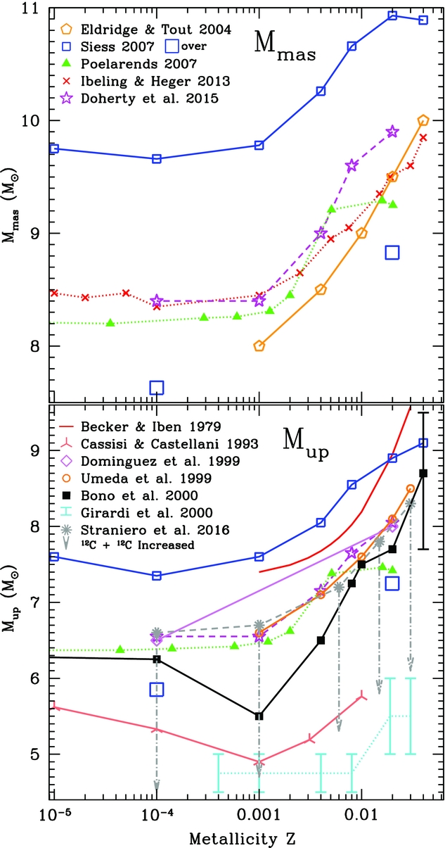
The mass boundaries M up and M mas are highly dependent on the maximum convective core mass obtained during CHB and CHeB. As can be seen in Section 2.2, the minimum CO core mass for carbon ignition is ~1.05 M⊙, whilst neon ignition requires ONe core masses ~1.37 M⊙.
3.1.1. The effect of the initial composition
Decreasing the stellar metallicity means decreasing the number of CNO nuclei and hence the efficiency of the CNO cycles. To maintain the required energy production for fewer CNO seeds, the stars attain higher central temperatures and luminosities during the main sequence phase of evolution. This results in a larger He core mass for the same initial mass and also more massive cores during CHeB, and hence results in more massive CO cores. Due to this, the M up values are seen to decrease with decreasing metallicity until reaching a plateau (or minimum e.g. Cassisi & Castellani Reference Cassisi and Castellani1993; Bono et al. Reference Bono, Caputo, Cassisi, Marconi, Piersanti and Tornambe2000) at about Z = 0.001 to 10−4. As can be seen in Figure 6, the behaviour of M mas with metallicity echoes that of M up albeit with an offset of about 1.5–2.1 M⊙ to higher initial masses.
Models that employ the strict Schwarzschild criterion for convective boundaries such as those from Siess (Reference Siess2007) typically produce the smallest HeB core, and hence represent a reasonable upper limit to the values of M up and M mas. For near solar composition (Z = 0.02) and using the strict Schwarzschild criterion, the M up and M mas values are ~9 and 11 M⊙, respectively (Garcia-Berro & Iben Reference Garcia-Berro and Iben1994; Ritossa et al. Reference Ritossa, García-Berro and Iben1999; Siess Reference Siess2007; Doherty et al. Reference Doherty, Siess, Lattanzio and Gil-Pons2010; Takahashi et al. Reference Takahashi, Yoshida and Umeda2013).
The values of M up and M mas also show large variations due to the He content (e.g. Becker & Iben Reference Becker and Iben1979; Bono et al. Reference Bono, Caputo, Cassisi, Marconi, Piersanti and Tornambe2000). Stars with larger initial He contents are more luminous and develop more massive convective cores during CHB. Their CHB lifetime is also substantially shorter due to both the reduced amount of H fuel and the hotter, larger cores that burn the fuel more efficiently. This larger core follows through to the CHeB phase resulting in a larger CO core that leads to a reduction of ~1.6–2 M⊙ in M up and M mas when enrichments of Y ~ 0.08–0.15 are used (e.g. Bono et al. Reference Bono, Caputo, Cassisi, Marconi, Piersanti and Tornambe2000; Shingles et al. Reference Shingles, Doherty, Karakas, Stancliffe, Lattanzio and Lugaro2015).
3.1.2. The effect of overshooting
Convective overshooting during the core H and He burning phases acts to mix additional fuel into the core. This increases the lifetime of these phases. It also increases the maximum size of the convective cores with this effect being more prominent during CHeB. With commonly used values of core overshoot, e.g. f over = 0.016, the M up and M mas values are generally reduced by about 2–2.5 M⊙ (e.g. Bertelli, Bressan, & Chiosi Reference Bertelli, Bressan and Chiosi1985; Siess Reference Siess2007; Gil-Pons, Gutiérrez, & García-Berro Reference Gil-Pons, Gutiérrez and García-Berro2007; Poelarends et al. Reference Poelarends, Herwig, Langer and Heger2008; Farmer et al. Reference Farmer, Fields and Timmes2015). This is highlighted in Figure 6 by comparing the large/small open square values from Siess (Reference Siess2007), which are for models with/without overshoot, respectively. We note that values of M mas from the recent literature that include convective overshooting are in reasonable agreement with these results. For example, for Z = 0.015, Woosley & Heger (Reference Woosley and Heger2015) find 9 M⊙, while Jones et al. (Reference Jones2013) find 8.8–9.5 M⊙ for Z = 0.02. However, even assuming the same convective approach during the pre-carbon burning phases, the M up values vary considerably between studies. For example, Girardi et al. (Reference Girardi, Bressan, Bertelli and Chiosi2000) find very low values of about 4.5–5 M⊙ at Z = 0.02. The causes of the differences are hard to attribute in some cases, as discussed in Siess (Reference Siess2007).
3.1.3. The effect of rotation
Stellar rotation has an impact similar to that of overshooting, in that it increases both the duration and the size of the convective core during CHB (e.g. Maeder & Meynet Reference Maeder and Meynet2000; Ekström et al. Reference Ekström2012). This larger core is then inherited by the CHeB phase, and hence we expect a larger CO core and presumably this would lead to a reduction in the initial mass for carbon ignition with increasing rotation rate. However, in their grid of intermediate-mass Z = 0.02 metallicity models with overshooting, Farmer et al. (Reference Farmer, Fields and Timmes2015) found that for a given initial mass, the CO core mass at carbon ignition was practically the same, irrespective of the initial rotation rate that ranged Ω/Ωcrit = 0–0.5 (their Figure 15). In this case, it seems the rotation does not impact the M up and M mas values provided that overshoot is efficient enough, and that rotation velocities are not close to their critical values.
3.1.4. Reaction rates
The rate of the 12C + 12C reactions can either hasten or delay the onset of C burning and hence alter the contraction time between He burning and C ignition. The CO core grows considerably during this phase and the impact of this should not be overlooked. The carbon burning 12C + 12C reaction rates can also modify the M up value. It has been suggested that there exists a possible unknown/unmeasured resonance (Spillane et al. Reference Spillane2007) that would increase the reaction rate above that currently recommended (Caughlan & Fowler Reference Caughlan and Fowler1988, hereafter CF88) and lead to a reduction in the core mass which ignites carbon, and hence reduces M up. Straniero, Piersanti, & Cristallo (Reference Straniero, Piersanti and Cristallo2016) examined the impact of including a narrow resonance at 1.45 MeV in the standard carbon burning rate. They found that the minimum CO core mass for carbon burning was shifted from ~1.06 M⊙ down to 0.95 M⊙, and this resulted in a uniform decrease of M up by about 2 M⊙ for their study over metallicities Z = 10−4−0.03. This can be seen in Figure 6 by the extent of the arrows representing models with the modified carbon burning rate. This reduction in M up with increased carbon reaction rate is in agreement with the results of Chen et al. (Reference Chen, Herwig, Denissenkov and Paxton2014). However, with their maximum rate (1 000 × CF88), they find a lesser decrease, at about 1.3 M⊙ (to M up ~ 5.3 M⊙ at metallicity Z = 0.01). In Fraser et al. (Reference Fraser2011), the M mas value was seen to decrease by 1 M⊙ (to 7 M⊙ at metallicity Z = 0.02) when the 12C + 12C reaction rates were enhanced by a factor of 105 compared to the standard CF88 rates.
Given the shape of the IMF and the decrease in M mas with decreasing metallicity, we expect that the SN rate was higher in the past. In summary, the two limiting masses M up and M mas are very uncertain and even with ‘reasonable’ choices of input physics their values may vary by over 3 M⊙. For example, at close to solar metallicity (Z = 0.02), M up can vary between about 5.5 and 9 M⊙. In Section 5, we discuss the observational probes that are being used to aid in constraining these important mass boundaries.
3.2. Final fates of super-AGB stars—M n
After SDU or dredge-out has reduced the core mass to below M Ch, the final fate of super-AGB stars is dictated by the competition between core growth and mass loss from the stellar envelope during the TP-SAGB phase. If the stellar wind removes the envelope prior to the core reaching M Ch, then the star will end its life as an ONe WD. Otherwise if the core growth is sufficient to reach M Ch, then the star will undergo an EC-SN and end its life as a neutron star. The boundary between these two differing final fates is called M n—the minimum mass for neutron star formation. We note here that the outcome of an EC-SN as a neutron star or as an ONeFe WD is debated e.g. Nomoto & Kondo (Reference Nomoto and Kondo1991); Isern et al. (Reference Isern, Canal and Labay1991); Canal, Isern, & Labay (Reference Canal, Isern and Labay1992); Jones et al. (Reference Jones, Röpke, Pakmor, Seitenzahl, Ohlmann and Edelmann2016b). If the fate of an EC-SN is not a neutron star, then M n=M mas.
Here, we describe the competing factors that determine the final fate including the complications from possible mass-ejection events, and summarise the results from both synthetic/parametric and detailed calculations that have examined this problem.
3.2.1. Core growth
The core growth rate during the super-AGB phase is dictated by the outward movement of the H burning shell and progresses at ~10−6 M⊙ yr−1 (Ritossa et al. Reference Ritossa, García-Berro and Iben1999; Poelarends et al. Reference Poelarends, Herwig, Langer and Heger2008; Siess Reference Siess2010; Doherty et al. Reference Doherty, Gil-Pons, Siess, Lattanzio and Lau2015) with typically faster growth rates in the more massive and/or metal-rich models.
An important factor that influences the effective core growth rate is the TDU. Unfortunately, whilst the efficiency of TDU is a very important quantity, it is also one of the most poorly constrained aspects of AGB modelling, especially at larger core masses. It depends on many factors such as the resolution (Straniero et al. Reference Straniero, Chieffi, Limongi, Busso, Gallino and Arlandini1997), numerics (Stancliffe, Tout, & Pols Reference Stancliffe, Tout and Pols2004; Stancliffe Reference Stancliffe2006), and treatment of convective boundaries (Frost & Lattanzio Reference Frost and Lattanzio1996; Herwig et al. Reference Herwig, Bloecker, Schoenberner and El Eid1997; Mowlavi Reference Mowlavi1999; Jones et al. Reference Jones, Ritter, Herwig, Fryer, Pignatari, Bertolli and Paxton2016a). As mentioned in Section 2.4, in super-AGB stars, the efficiency of TDU varies considerably between studies and ranges from λ = 0 to λ > 1, typically being smaller for more massive models. There is some evidence for TDU in massive AGB stars of high metallicities. This is in the form of Rb over-abundances observed in bright O-rich AGB stars in the Galaxy and Magellanic Clouds (García-Hernández et al. Reference García-Hernández, García-Lario, Plez, D’Antona, Manchado and Trigo-Rodríguez2006, Reference García-Hernández2009). The existence of very luminous carbon rich stars in the Magellanic Clouds is suspected to arise from TDU events after the cessation of HBB (Frost et al. Reference Frost, Cannon, Lattanzio, Wood and Forestini1998; van Loon, Zijlstra, & Groenewegen Reference van Loon, Zijlstra and Groenewegen1999). Unfortunately, we are yet to unambiguously identify any super-AGB stars (see Sections 5.1 and 5.3), and there are no constraints from lower metallicity objects, because such stars have long since died. A standard tracer of AGB nucleosynthesis is 99Tc, which is produced by neutron captures in the deep layers of the star. Technetium has no stable isotope, and its longest lived isotope is 99Tc with a half-life of 0.21 Myr. Therefore, the detection of Tc in the stellar spectra is the signature of recent nucleosynthetic activity and the presence of TDU. Unfortunately, super-AGB stars are not expected to be able to produce large enough amounts of Tc for it to be observable (e.g. from the massive AGB stars study by García-Hernández et al. Reference García-Hernández, Zamora, Yagüe, Uttenthaler, Karakas, Lugaro, Ventura and Lambert2013).
3.2.2. Mass loss and mass ejections
Whilst the mass-loss rate is fundamental to determining the final fates of super-AGB stars, unfortunately it is also highly uncertain especially at lower metallicities. Mass loss in (super-)AGB stars is thought to be via pulsation aided dust-driven winds. First, large amplitude pulsations are responsible for forcing material to large enough radii and increasing the density enough for dust grains to form. The radiation pressure from the star is then able to accelerate these dust particles which are collisionally coupled to the gas, leading to quite efficient mass loss (Wood Reference Wood1979). Although there is no mass-loss rate derived specifically for super-AGB stars, it is common to use rates derived for lower mass AGB stars (e.g. Vassiliadis & Wood Reference Vassiliadis and Wood1993; Bloecker Reference Bloecker1995), or for rates taken from red super-giant and O-rich AGB stars (van Loon et al. Reference van Loon, Cioni, Zijlstra and Loup2005). Using these prescriptions, the mass-loss rates in super-AGB stars are of the order 10−4–10−5 M⊙ yr−1.
The mass-loss rate for super-AGB stars at low metallicity is unknown and we can only apply prescriptions that were derived using observations of solar metallicity, or moderately metal-poor stars. Due to their more compact structure, low metallicity stars are expected to have slower mass-loss rates. Kudritzki, Pauldrach, & Puls (Reference Kudritzki, Pauldrach and Puls1987) proposed a metallicity scaling proportional to $\sqrt{Z/Z_\odot }$
in an attempt to take this into account. We note however that this scaling was derived for radiative line-driven winds of hot luminous O stars whose conditions are quite unlike the cool super-AGB stars we are considering here.
$\sqrt{Z/Z_\odot }$
in an attempt to take this into account. We note however that this scaling was derived for radiative line-driven winds of hot luminous O stars whose conditions are quite unlike the cool super-AGB stars we are considering here.
Another important factor that determines the mass-loss rate in super-AGB stars is the envelope opacity. The use of low temperature molecular opacities that take into account the envelope composition variations is crucial for cases where the envelope molar abundance ratio C/O exceeds unity. The change in molecular chemistry when a star becomes carbon rich leads to an increase in opacity, which results in a cooler and more extended stellar envelope and a higher mass-loss rate (Marigo Reference Marigo2002; Cristallo et al. Reference Cristallo, Straniero, Lederer and Aringer2007; Ventura & Marigo Reference Ventura and Marigo2010; Constantino et al. Reference Constantino, Campbell, Gil-Pons and Lattanzio2014; Doherty et al. Reference Doherty, Gil-Pons, Lau, Lattanzio, Siess and Campbell2014b). This effect may play an important role for low metallicity super-AGB stars. This is especially true for the most massive super-AGB stars, with post-SDU/dredge-out core masses closest to M Ch. These stars have often had their surface enriched in C due to dredge-out events and are already carbon rich (with C/O > 10 in some cases) at the start of the TP-SAGB phase.
The final fates of metal poor super-AGB stars are also strongly influenced by the efficiency of SDU/dredge-out prior to the TP-SAGB phase. These processes are able to mix significant amounts of metals from the stellar interior leading to surface metallicities up to Z ≈ 0.001, with the amount of enrichment increasing with stellar mass (Gil-Pons et al. Reference Gil-Pons, Doherty, Lau, Campbell, Suda, Guilani, Gutiérrez and Lattanzio2013). Furthermore, the nucleosynthesis and mixing processes that occur during the TP-SAGB also alter their total surface metallicity. As a consequence, their envelope opacity values, surface luminosities and radii become very similar to their higher Z counterparts. Envelope metallicity during the TP-SAGB is critical in terms of the strength of stellar winds, as higher Z objects are thought to be able to drive higher mass-loss rates.
At low metallicities, if the mass-loss rate is sufficiently low, there is the possibility for stars with initial masses below M up to be able to grow enough to reach M Ch and explode as a Type 1.5 SN (Arnett Reference Arnett1969; Iben & Renzini Reference Jr and Renzini1983; Zijlstra Reference Zijlstra2004; Gil-Pons et al. Reference Gil-Pons, Gutiérrez and García-Berro2007; Lau, Stancliffe, & Tout Reference Lau, Stancliffe and Tout2008; Wood Reference Wood, Qain, Leung, Zhu and Kwok2011). This class of SN is suspected to occur when a degenerate CO core within an AGB star grows to the Chandrasekhar mass prior to removal of its envelope. Carbon is then ignited under conditions such that the thermonuclear runaway will lead to an explosion that will disrupt the entire star. Due to the massive H-rich envelope, the early light curve should resemble that of a Type II SN; however, due to the production of a substantial amount of radioactive Ni within the explosion, the resultant light curve will also have a late exponential luminosity decline reminiscent of a Type Ia SN.
In addition to standard super-wind mass loss from super-AGB stars, there have also been two suggested potential mass expulsions events, from either the Fe-peak instability (Lau et al. Reference Lau, Gil-Pons, Doherty and Lattanzio2012) or as a result of convective-reactive H-ingestion events (Jones et al. Reference Jones, Ritter, Herwig, Fryer, Pignatari, Bertolli and Paxton2016a). These phenomena are expected to occur at different evolutionary phases, with the Fe-instability generally seen near the end stages of the TP-(S)AGB when the envelope has reduced below about 3M⊙, whilst convective-reactive H-ingestion episodes and potential mass ejection could occur prior to the start of the thermally pulsing phase during the dredge-out phase. These types of mass ejections make determining the final fates of super-AGB stars, in particular the most massive near the EC-SN boundary, quite problematic.
3.2.3. Structural models and/or population synthesis
Whilst the final fates of thermally pulsing super-AGB stars had been examined for individual models of Z = 0.02 in the pioneering series of papers by Garcia-Berro, Iben and Ritossa (Garcia-Berro & Iben Reference Garcia-Berro and Iben1994; Ritossa et al. Reference Ritossa, Garcia-Berro and Iben1996; Garcia-Berro, Ritossa, & Iben Reference Garcia-Berro, Ritossa and Iben1997; Iben, Ritossa, & Garcia-Berro Reference Iben, Ritossa and Garcia-Berro1997; Ritossa et al. Reference Ritossa, García-Berro and Iben1999), the global final fates problem for super-AGB stars was first tackled in a parametric fashion by Poelarends (Reference Poelarends2007), Poelarends et al. (Reference Poelarends, Herwig, Langer and Heger2008) and Siess (Reference Siess2007), with each of these studies using slightly different approaches.
In Poelarends (Reference Poelarends2007), a suite of synthetic models was computed exploring the rate of EC-SNe when using differing mass-loss rates (Vassiliadis & Wood Reference Vassiliadis and Wood1993; van Loon et al. Reference van Loon, Cioni, Zijlstra and Loup2005), efficiencies of TDU and a metallicity scaling included in the mass-loss rate. The final fate results from their best estimate, which included the mass loss prescription from van Loon et al. (Reference van Loon, Cioni, Zijlstra and Loup2005), parameterised TDU from Karakas, Lattanzio, & Pols (Reference Karakas, Lattanzio and Pols2002), and metallicity scaling of Kudritzki et al. (Reference Kudritzki, Pauldrach and Puls1987), are shown in the top panel of Figure 7 (which is adapted from Figure 12 in Langer Reference Langer2012). This figure includes the critical mass limits delineating different evolutionary fates. We define ΔM
EC-SN and ΔM
ONe as the range of initial masses that produces EC-SNe and ONe WDs respectively. For Z = 0.02, this EC-SN channel is narrow with $\Delta M_{\rm {EC\text{-}SN}}$
~ 0.2 M⊙, but at the lowest metallicity, all super-AGB stars would end life as EC-SNe, giving
$\Delta M_{\rm {EC\text{-}SN}}$
~ 0.2 M⊙, but at the lowest metallicity, all super-AGB stars would end life as EC-SNe, giving $\Delta M_{\rm {EC\text{-}SN}}$
~ 1.8 M⊙, and leaving no ONe WDs. Interestingly at Z = 10−5 even the most massive CO cores are able to grow to M
Ch and explode as Type 1.5 SN. The cause of this increase in the EC-SN rate with decreasing metallicity is primarily the application of the metallicity scaling on the mass-loss rate. In the case with no metallicity scaling applied to the mass loss (dashed line in Figure 7), they find
$\Delta M_{\rm {EC\text{-}SN}}$
~ 1.8 M⊙, and leaving no ONe WDs. Interestingly at Z = 10−5 even the most massive CO cores are able to grow to M
Ch and explode as Type 1.5 SN. The cause of this increase in the EC-SN rate with decreasing metallicity is primarily the application of the metallicity scaling on the mass-loss rate. In the case with no metallicity scaling applied to the mass loss (dashed line in Figure 7), they find $\Delta M_{\rm {EC\text{-}SN}} \sim 0.25$
–0.55 M⊙ with the wider range at lower metallicity.
$\Delta M_{\rm {EC\text{-}SN}} \sim 0.25$
–0.55 M⊙ with the wider range at lower metallicity.
Final fates of intermediate-mass stars from Poelarends (Reference Poelarends2007) (top panel) and Doherty et al. (Reference Doherty, Gil-Pons, Siess, Lattanzio and Lau2015) (bottom panel). Solid lines delineate M up, M n, and M mas. The dashed line in the top panel represents the M n value in the case where no metallicity factor is applied to the mass-loss rate. The hatched region represents the width of the EC-SNe channel. As mentioned in Section 3.1, there is a slight offset in the M up and M mas values between the two sets of models, with this due to the different method for treatment of convective boundaries during CHeB: Poelarends (Reference Poelarends2007) included convective overshooting via the method of Herwig et al. (Reference Herwig, Bloecker, Schoenberner and El Eid1997) with an overshoot parameter of f over = 0.016, whilst Doherty et al. (Reference Doherty, Gil-Pons, Siess, Lattanzio and Lau2015) used the search for convective neutrality approach of Lattanzio (Reference Lattanzio1986). We note that if no super-AGB stars become EC-SN, then M n=M mas. It is also worth noting that M n will always be greater than M up because even if explosions of CO cores occur (the Type 1.5 SNe), they are not expected to leave neutron star remnants. The lowest metallicity examined in Doherty et al. (Reference Doherty, Gil-Pons, Siess, Lattanzio and Lau2015) was Z = 10−4, but here we present new models for Z = 10−5 calculated using the same methodology as in the previous work.

Also critical to the width of the EC-SN channel is the occurrence of TDU, with lower efficiencies resulting in a wider channel. However, we expect the impact of the metallicity scaling upon the mass-loss rate to be greater than the possible lack of TDU. In Poelarends et al. (Reference Poelarends, Herwig, Langer and Heger2008), the width of the EC-SN channel was explored for solar metallicity using a selection of commonly used mass-loss rates (Reimers Reference Reimers1975; Vassiliadis & Wood Reference Vassiliadis and Wood1993; Bloecker Reference Bloecker1995; van Loon et al. Reference van Loon, Cioni, Zijlstra and Loup2005) as well as the efficiency of TDU, finding $\Delta M_{\rm {EC\text{-}SN}}$
ranging from ~0.2–1.4 M⊙. For a rough estimation, the order of increasing mass-loss rate is the following: Reimers (Reference Reimers1975) (with η = 5), van Loon et al. (Reference van Loon, Cioni, Zijlstra and Loup2005), Vassiliadis & Wood (Reference Vassiliadis and Wood1993) and Bloecker (Reference Bloecker1995) (with η = 0.1), with approximate values for a typical metal-rich super-AGB star being 0.2, 0.4, 0.8 and 3 × 10⁻⁴ M⊙ yr−1, respectively (see Figure 7 in Doherty et al. Reference Doherty, Gil-Pons, Lau, Lattanzio and Siess2014a).
$\Delta M_{\rm {EC\text{-}SN}}$
ranging from ~0.2–1.4 M⊙. For a rough estimation, the order of increasing mass-loss rate is the following: Reimers (Reference Reimers1975) (with η = 5), van Loon et al. (Reference van Loon, Cioni, Zijlstra and Loup2005), Vassiliadis & Wood (Reference Vassiliadis and Wood1993) and Bloecker (Reference Bloecker1995) (with η = 0.1), with approximate values for a typical metal-rich super-AGB star being 0.2, 0.4, 0.8 and 3 × 10⁻⁴ M⊙ yr−1, respectively (see Figure 7 in Doherty et al. Reference Doherty, Gil-Pons, Lau, Lattanzio and Siess2014a).
In Siess (Reference Siess2007), post-SDU/dredge-out core masses were taken from detailed calculations and then the further evolution during the TP-SAGB phase was extrapolated based on the ratio of the average envelope mass-loss rates $\dot{M}_{\rm {env}}$
to average effective core growth rates
$\dot{M}_{\rm {env}}$
to average effective core growth rates $\dot{M}_{\rm {core}}$
characterised by a ζ parameter defined as
$\dot{M}_{\rm {core}}$
characterised by a ζ parameter defined as $\zeta =\mid {\frac{\dot{M}_{\rm {env}}}{\dot{M}_{\rm {core}}}}\mid$
. With best estimate values of
$\zeta =\mid {\frac{\dot{M}_{\rm {env}}}{\dot{M}_{\rm {core}}}}\mid$
. With best estimate values of $\dot{M}_{\rm {core}} = 5 \times 10^{-7}$
M⊙ yr−1, TDU efficiency λ values between 0.3–0.9, and with
$\dot{M}_{\rm {core}} = 5 \times 10^{-7}$
M⊙ yr−1, TDU efficiency λ values between 0.3–0.9, and with $\dot{M}_{\rm {env}}$
= 5 × 10⁻⁵ M⊙ yr−1, the ζ values range from 140–1000. With these values, the
$\dot{M}_{\rm {env}}$
= 5 × 10⁻⁵ M⊙ yr−1, the ζ values range from 140–1000. With these values, the $\Delta M_{\rm {EC\text{-}SN}}$
ranged from ~ 0.1 M⊙ (ζ = 1000) to ~0.25–0.6 M⊙ (ζ = 100) with these widths relatively constant over the entire metallicity range Z = 0.04–10−5. When the metallicity scaling of Kudritzki et al. (Reference Kudritzki, Pauldrach and Puls1987) was applied to the mass-loss rate, a very similar result to that of Poelarends (Reference Poelarends2007) was found with
$\Delta M_{\rm {EC\text{-}SN}}$
ranged from ~ 0.1 M⊙ (ζ = 1000) to ~0.25–0.6 M⊙ (ζ = 100) with these widths relatively constant over the entire metallicity range Z = 0.04–10−5. When the metallicity scaling of Kudritzki et al. (Reference Kudritzki, Pauldrach and Puls1987) was applied to the mass-loss rate, a very similar result to that of Poelarends (Reference Poelarends2007) was found with $\Delta M_{\rm {EC\text{-}SN}}$
increasing substantially at lower metallicity, and at Z = 10−5, the ONe WD channel disappears entirely.
$\Delta M_{\rm {EC\text{-}SN}}$
increasing substantially at lower metallicity, and at Z = 10−5, the ONe WD channel disappears entirely.
Using detailed evolutionary calculations, Doherty et al. (Reference Doherty, Gil-Pons, Siess, Lattanzio and Lau2015) confirmed the results of these earlier parametric studies. They found that when using reasonable mass-loss rates (Vassiliadis & Wood Reference Vassiliadis and Wood1993), without an explicit metallicity scaling but with efficient TDU, the width of the EC-SN channel from super-AGB stars is narrow with $\Delta M_{\rm {EC\text{-}SN}}$
~0.1–0.2 M⊙(bottom panel of Figure 7). This figure shows that the vast majority of stars that enter the TP-SAGB phase will end life as ONe WDs, in sharp contrast with the favoured set by Poelarends (Reference Poelarends2007).
$\Delta M_{\rm {EC\text{-}SN}}$
~0.1–0.2 M⊙(bottom panel of Figure 7). This figure shows that the vast majority of stars that enter the TP-SAGB phase will end life as ONe WDs, in sharp contrast with the favoured set by Poelarends (Reference Poelarends2007).
By taking the mass range of the EC-SN channel and weighting it with an IMF, the importance and fractional contribution towards the overall core-collapse supernova rate can be determined. Using a Salpeter IMF and the EC-SN, width and mass limits from the synthetic calculations of Poelarends (Reference Poelarends2007) result in 5%, 17% and 38% of all Type II-P SNe coming from the EC-SN channel for metallicities Z = 0.02, 0.001 and 10−5, respectively. For our calculations, we assumed that the maximum mass for a Type II-P SN is 18M⊙ based on the analysis of SN observations by Smartt (Reference Smartt2015).
In contrast to using the results from Doherty et al. (Reference Doherty, Gil-Pons, Siess, Lattanzio and Lau2015) over these same metallicities, we find a far smaller percentage, of about 2–5% of all Type II-P SNe will be EC-SNe. This large variation in frequency of EC-SNe highlights the importance of constraining the mass-loss rate at low metallicity.
We note here that models that undergo core overshooting will have far smaller envelopes (by as much as 2–3 M⊙) to remove in order for a star to avoid the EC-SN channel. This will result in fewer SNe for models with larger values of overshooting.
3.3. The binary channels towards EC-SNe
The calculations presented in the previous section have shown that the EC-SN channel for single super-AGB stars strongly depends on the mass-loss rate and the efficiency of the TDU, both of which are highly uncertain and remain poorly constrained. Standard prescriptions for the wind mass-loss rate usually have no explicit dependence on metallicity. Nevertheless the metallicity is implicitly included via its effect on the structural variables that appear in the formula. Using such standard formulae, Siess (Reference Siess2007), Poelarends et al. (Reference Poelarends, Herwig, Langer and Heger2008) and Doherty et al. (Reference Doherty, Gil-Pons, Siess, Lattanzio and Lau2015) showed that the initial mass range for single stars to evolve toward EC-SNe is narrow, being of the order of 0.1–0.5 M⊙. However, this picture does not consider binary evolution, which opens new channels for the formation of such SNe and ONe WDs. This is particularly relevant considering the high fraction of stars having a companion Raghavan et al. (Reference Raghavan2010) and that about 70% of all stars more massive than 15M⊙ will interact at some point with a binary companion Sana et al. (Reference Sana2012).
We will start our discussion with the accretion onto an ONe WD in a short period system. These systems represent the massive counterparts of cataclysmic variables and follow a similar evolutionary scenario for their formation but with different initial conditions (for a review on the formation of cataclysmic variables see e.g. Ritter Reference Ritter2012). The evolution starts with a super-AGB progenitor and a lower-mass companion. If the initial period is long enough, mass transfer by Roche lobe overflow starts when an ONe core is formed and the super-AGB star has entered the TP-SAGB phase. Because the super-AGB star has a deep convective envelope, mass transfer is likely to become dynamically unstableFootnote 7 resulting in the formation of a common envelope. When the mass transfer timescale becomes shorter than the thermal timescale of the accreting component, the gainer star cannot assimilate the incoming material and the matter ejected from the mass-losing star soon engulfs the binary system. The energy dissipated by the stars within the gaseous envelope will produce a spiralling-in with transfer of orbital angular momentum and potential energy to the envelope. The outcome of this process is either the merger of the two stars if the envelope is not ejected sufficiently rapidly or the formation of a short(er) period binary system if the common envelope is rapidly dispersed. This phase is short lived (~1000 yr) and during that short period of time, the companion is not expected to accrete a significant amount of mass. Today, the determination of final orbital parameters is still subject to large uncertainties associated with our understanding of the energetics involved (for a review of common envelope evolution see Ivanova et al. Reference Ivanova2013).
If the system avoids merging, we are left with a detached system. The hot core of the super-AGB star ionizes the expanding envelope, enabling it to shine for ~104 yr as a planetary nebula. Subsequently, the companion may fill its Roche lobe driving a second phase of (reversed) mass transfer. This can be initiated either by the star expanding as a result of its nuclear evolution, or by the loss of orbital angular momentum due to gravitational wave emission and/or magnetic coupling.
On the other hand, for shorter periods, mass transfer may be initiated while the super-AGB star progenitor is on the red giant branch. Because of the extended convective envelope, this case B Roche lobe overflow is unstable and, for the reason mentioned before, a common envelope develops. The H-rich envelope of the primary is ejected and the outcome is the formation of a short period system composed of a naked He star and a low-mass companion. The evolution of this post-common-envelope binary has been investigated by Law & Ritter (Reference Law and Ritter1983) and detailed stellar models were computed by Dominguez, Tornambe, & Isern (Reference Dominguez, Tornambe and Isern1993) and Gil-Pons & García-Berro (Reference Gil-Pons and García-Berro2001, Reference Gil-Pons and García-Berro2002). These simulations indicate that a second episode of mass transfer is triggered after the onset of He shell burning (referred to as case BB) and because the He star has a radiative envelope, the mass loss from the primary is stable. In their study of a 10 M⊙ primary with a lower-mass companion, Gil-Pons & García-Berro (Reference Gil-Pons and García-Berro2001) showed that the second mass transfer episode is stable and that the system detaches when carbon ignites leading to the formation of a cataclysmic variable with an ONe WD. On the other hand, starting with a 9 M⊙ initial model, the primary loses so much mass that it does not ignite carbon and ends up as a CO WD (Gil-Pons & García-Berro Reference Gil-Pons and García-Berro2002).
The fate of the accreting WD depends mainly on the mass-accretion rate (e.g. Nomoto Reference Nomoto1982): if it is too low, recurrent H shell flashes (nova outbursts) eject more mass than has been accreted and the accretor loses mass. On the other hand if the accretion rate is higher than the core growth rate (which is controlled by the H-burning shell), then the accreted envelope expands and a common envelope may ensue followed by a spiral-in phase. In the intermediate regime, H burning is steady, and stable accretion allows the ONe core to grow. When the central density reaches 4 × 10⁹ g cm−3 for an ONe core mass of ~1.37 M⊙ Nomoto (Reference Nomoto1984), electron capture reactions on 24Mg, 24Na and 20Ne are successively activated. They induce the collapse of the white dwarf and the heat released by γ-ray emission ignites oxygen burning. The outcome of this accretion-induced collapse depends on whether or not the timescale for electron capture (which induces contraction) is shorter than the timescale associated with the nuclear energy release by oxygen burning (which produces expansion). As mentioned in Section 1, the competition between these two processes is sensitive to the density where nuclear burning is ignited, and whilst the more traditional viewpoint suggests the final fate of an ONe core accretion-induced collapse leads to the formation of a neutron star rather than a thermonuclear explosion, this is still an open problem (e.g. Jones et al. Reference Jones, Röpke, Pakmor, Seitenzahl, Ohlmann and Edelmann2016b).
Binary evolution opens new possibilities and in particular that the formation of an ONe WD or EC-SN does not necessarily require a super-AGB star progenitor. The proposed scenario considers the merging of two CO WDs. The formation of such systems has been investigated by Iben & Tutukov (Reference Jr and Tutukov1984) and Webbink (Reference Webbink1984) and involves one or two common envelope episodes. Once the two WDs are formed in a short period system, angular momentum loss by gravitational wave radiation brings the two cores closer to each other. Eventually, the lower-mass WD, which has the largest radius, starts overfilling its Roche lobe and is eventually disrupted by the strong tidal forces. The material distributes in a thick accretion disk around the massive WD and mass transfer of hot CO material onto the surviving companion begins. The mass-transfer rate is then expected to be very high, of the order of 10−5 M⊙ yr−1, and close to the Eddington limit. As initially investigated by Saio & Nomoto (Reference Saio and Nomoto1985), in this double degenerate scenario, the fast accretion leads to off-center ignition of carbon and the inward propagation of a burning front that incinerates the CO WD into an ONe core that may eventually collapse into a neutron star if it is massive enough. However, this picture is oversimplified. Hydrodynamical simulations (e.g. Guerrero, García-Berro, & Isern Reference Guerrero, García-Berro and Isern2004; Pakmor et al. Reference Pakmor, Edelmann, Röpke and Hillebrandt2012) reveal that soon after the disruption of the WD, a ‘quasi-static’ configuration develops in which the cold WD core is enshrouded in a hot, rapidly rotating CO envelope surrounded by a thick Keplerian disk. Using these new and more realistic initial conditions, Yoon, Podsiadlowski, & Rosswog (Reference Yoon, Podsiadlowski and Rosswog2007) re-investigated the conditions for off-centre carbon ignition and showed that it depends on the temperature in the hot envelope, the mass-accretion rate and the mass of the WD. Recent 3D SPH simulations (e.g. Sato et al. Reference Sato, Nakasato, Tanikawa, Nomoto, Maeda and Hachisu2016, and reference therein) also predict that the outcome, accretion-induced collapse or Type Ia explosion, depends sensitively on the initial mass ratio.
The evolution of single super-AGB stars tell us that the SDU can significantly reduce the mass of the H-exhausted core below the Chandrasekhar limit as illustrated in Figure 3. Models also show that the core growth during the subsequent TP-SAGB phase is very modest and that very few stars reach the conditions for EC-SNe. This prompted Podsiadlowski et al. (Reference Podsiadlowski, Langer, Poelarends, Rappaport, Heger and Pfahl2004) to suggest that binary interaction may be able to remove the envelope before the SDU occurs and thus allows more super-AGB stars to become EC-SNe.
In some early papers, Nomoto (Reference Nomoto1984, Reference Nomoto1987) investigated the fate of He cores representative of the evolution of 8–10 M⊙ models and showed that for He core masses in the range 2–2.5 M⊙, the evolution proceeds towards EC-SNe. Therefore, a new channel to EC-SNe will open if, at the end of a case A or B mass transfer, the super-AGB donor keeps a helium core mass in the range 2–2.5 M⊙. However, Podsiadlowski et al. (Reference Podsiadlowski, Langer, Poelarends, Rappaport, Heger and Pfahl2004) also pointed out that this simple picture does not take into account the effects of binary interactions that can substantially alter the stellar structure. In particular, the size of the helium core depends on the mass of the hydrogen envelope. Previous studies (e.g. Wellstein & Langer Reference Wellstein and Langer1999; Gil-Pons et al. Reference Gil-Pons, García-Berro, José, Hernanz and Truran2003a) indeed show that the helium core mass can be dramatically reduced in short period systems compared to the evolution of a single star. Furthermore, binary interactions contribute to redistributing the angular momentum inside the star. This is likely to generate additional mixing that will also affect the He core mass. This promising scenario remains to be explored with the self-consistent models, so that the range of initial periods and stellar masses can be identified.
Investigating the origin of unusual fast and faint optical transients, Tauris et al. (Reference Tauris, Langer, Moriya, Podsiadlowski, Yoon and Blinnikov2013), Tauris, Langer, & Podsiadlowski (Reference Tauris, Langer and Podsiadlowski2015) studied the evolution of binary systems composed of a neutron star orbiting a helium-star companion. This initial set-up is the result of previous binary evolution that can be summarised as follows. The starting point is two main sequence stars with the primary being a typical B star (3 M⊙ ≲ M1 ≲ 20 M⊙). Depending on the initial period and mass ratio, the more massive component undergoes Roche lobe overflow while on the main sequence (case A) or after core H-exhaustion (case B). As a result of this conservative mass transfer, the system is composed of a naked He-star (the initially more massive star stripped of its H-rich envelope) and a relatively massive (8 M⊙ ≲ M2 ≲ 20 M⊙) main sequence companion (which has accreted a substantial fraction of the primary’s envelope) in a wide orbit. The more evolved He star eventually explodes as a supernovae (possibly an EC-SN!) leaving a neutron star remnant. If the explosion does not disrupt the system, the neutron star can accrete some of the wind from the secondary (likely a Be star) and may show up as an X-ray source. Thereafter, the secondary fills its Roche lobe but because of the extreme mass ratio, mass transfer is dynamically unstable and leads to common-envelope evolution. After spiral-in, and provided merging is avoided, the final system consists of a short-period neutron star orbiting the naked He core of the secondary. The subsequent evolution is similar to the previous one. After core He exhaustion, the He-star expands and a new episode of mass transfer begins (Habets Reference Habets1986; Dewi et al. Reference Dewi, Pols, Savonije and van den Heuvel2002), which is temporarily halted during central C burning. At this stage, the exchange of mass is highly non-conservative because the mass-transfer rate is 3–4 orders of magnitude larger than the Eddington accretion limit of the neutron star (a few 10−8 M⊙ yr−1). In their study, Tauris et al. (Reference Tauris, Langer and Podsiadlowski2015) showed that by gradually increasing the initial period (from 0.06 to 2.0 days) and the mass of the He-star, the remnant of the He-star varies from CO WD to ONe WD, to neutron stars formed by EC-SN or FeCC-SN as a consequence of mass transfer occurring during core helium burning (case BA), He shell burning (case BB), or beyond (case BC). In some cases, the mass transfer runs away and a common-envelope episode follows leading to a merger or the formation of a very tight system. In this scenario, EC-SN will mainly be observed as weak Type Ic SNe.
4 SUPER-AGB STAR NUCLEOSYNTHESIS
A variety of mixing episodes can occur in intermediate-mass stars prior to the TP-SAGB phase. Super-AGB stars of high and moderate metallicities (Z ≳ 0.001) undergo the first dredge-up event that mixes material to the surface from regions that have undergone partial hydrogen burning. This matter has experienced partial CNO cycling but with only marginal activation of the heavier hydrogen burning cycles/chains. There are increases in the surface abundances of 4He, 14N, 13C, 17O and to a lesser extent increases in 23Na, 21Ne, and 26Mg. Simultaneously there is a decrease in the surface abundances of H, 7Li, 12C, 15N, and 18O.
As with the FDU, SDU mixes to the surface species involved in H burning, with the main nucleosynthetic signature being a very large enhancement of 4He by up to ~0.1 in mass fraction and also significant surface enrichment of 14N and 23Na. In addition to the enrichment from standard SDU, models with corrosive SDU also increase the surface abundance of 12C, and in some cases 16, 18O and 22Ne. Dredge-out events also have the ability to enrich the surface in products of partial He burning, in particular 12C. As mentioned in Doherty et al. (Reference Doherty, Gil-Pons, Siess, Lattanzio and Lau2015) and Jones et al. (Reference Jones, Ritter, Herwig, Fryer, Pignatari, Bertolli and Paxton2016a), the 13C produced via proton capture on 12C will subsequently undergo the 13C(α,n)16O reaction with the neutrons so produced leading to potentially significant heavy element production.
Once the star reaches the TP-SAGB phase, the nucleosynthesis is dictated by hot bottom burning and (potentially) third dredge-up.
4.1. Hot bottom burning
Hot bottom burning (hereafter HBB) occurs during the interpulse phase when the material in a very thin region at the base of the convective envelope is hot enough to undergo nuclear burning. An equivalent, and perhaps more intuitive, way to think of this is that the bottom of the convective envelope extends into the top of the H-burning shell. The maximum temperature found at the bottom of the envelope is a function of initial metallicity and mass, with more massive and/or metal-poor models achieving higher temperatures. For super-AGB stars this temperature ranges from about 100–160 × 106 K with a density of about 10 g cm−3. With such high temperatures there is activation of the CNO, Ne–Na, Mg–Al chains/cycles and potentially proton-capture reactions involving heavier species such as Ar and K (see Figure 8).
A section of the chart of the nuclides (with atomic mass number on the x-axis and proton number on the y-axis) showing the CNO and Ne–Na cycles and Mg–Al and Ar–K chains. Solid circles denote stable isotopes whilst dashed squares show unstable isotopes.

Another consequence of HBB in super-AGB stars is the activation of the Cameron-Fowler mechanism (Cameron & Fowler Reference Cameron and Fowler1971). Here, 7Be is created from 4He(3He,γ)7Be and is quickly mixed to a cooler region where it undergoes electron capture to form 7Li. Super-AGB stars can indeed become very lithium rich, with A(7Li) up to ~4.5Footnote 8 , for a short time at the start, or just prior to the TP-SAGB phase. But once the 3He in the envelope is depleted the Li production ceases and Li is efficiently destroyed. HBB also produces 4He, but unless the TP-SAGB phase is very extended, the main contribution to the surface of 4He will remain SDU/dredge-out.
Activation of the CNO cycles leads to the production of 13C and 14N to the detriment of 12C, with this efficient destruction being able to decrease the C/O ratio to below unity in the cases where the surface has been enriched from corrosive SDU, dredge-out or efficient TDU. However, at high temperatures exceeding 95 × 106 K the 16O(p,γ)17F channel opens and depletes 16O. In the most metal-poor/massive super-AGB star models, this can lead to the creation of a carbon star (C/O > 1) not from C enrichment but from the depletion of O (Siess Reference Siess2010). The 12C/13C and 14N/15N number ratios reach their equilibrium values.
Within the Ne–Na cycle very hot HBB leads to the destruction of 21, 22Ne and 23Na to the benefit of the already very abundant 20Ne.
For super-AGB stars, the most obvious result from the Mg–Al burning is the very large reduction of 24Mg, which is almost completely destroyed to form 25Mg. 26Al is also produced (Siess & Arnould Reference Siess and Arnould2008; Doherty et al. Reference Doherty, Gil-Pons, Lau, Lattanzio and Siess2014a) but at these high temperatures the 26Al(p,γ)27Si(β+)27Al channel opens, which bypasses the 26Mg. As the temperatures increase beyond 110 × 106 K there is activation of the 27Al(p,γ)28Si reaction (Ventura, Carini, & D’Antona Reference Ventura, Carini and D’Antona2011).
If the HBB temperatures in super-AGB stars are extreme (exceeding 150 × 106 K) the argon–potassium (Ar–K) chain (refer Figure 8) may also be activated (Ventura et al. Reference Ventura, D’Antona, Di Criscienzo, Carini, D’Ercole and Vesperini2012c), with this chain being potentially of particular relevance to the globular cluster abundance anomaly problem (refer to Section 4.5).
We note here that the temperature at the base of the convective envelope is strongly influenced by the theory of convection that is used. Models such as those by Ventura & D’Antona (Reference Ventura and D’Antona2005) and Ventura et al. (Reference Ventura, Carini and D’Antona2011), which use the full spectrum of turbulence model (hereafter the FST model, see Canuto & Mazzitelli Reference Canuto and Mazzitelli1991), attain higher temperatures for the same initial mass when compared to models that use standard mixing length theory.
The nuclear reaction rates are also a source of great uncertainty in these heavier proton chains and this can lead to substantial differences between results depending on which reaction rates are used, in particular the linking reactions between the chains/cycles such as 23Na(p,α)20Ne.
Near the end of evolution when the envelope mass drops below about 1–2 M⊙, the temperature reduces below the critical value required to sustain HBB and this process ceases.
4.2. Third dredge up
Within the intershell convective zone during a thermal pulse the main product is 12C produced by the triple-α reaction with subsequent production also of the α capture species 16O, 20Ne, 24Mg, and 28Si. The abundant 14N in the intershell from the preceding CNO cycling is converted to 22Ne through the reactions 14N(α, γ)18F(β+ν)18O(α, γ)22Ne. Due to the large temperature in the helium burning intershell convective zone, the 22Ne(α,n)25Mg and 22Ne(α, γ)26Mg reactions are activated. There is a substantial neutron flux resulting from the 22Ne(α,n)25Mg reaction with neutron densities of up to 1014 − 15 cm−3. These free neutrons can be captured by Fe (and other) seeds within the convective pulse and lead to heavy element production via the slow (s) neutron capture process.
Relevant to heavy element production in super-AGB stars is the occurrence of hot TDU events, where the temperature at the base of the convective envelope during the TDU is still high enough for nuclear burning to be active (e.g. Chieffi et al. Reference Chieffi, Domínguez, Limongi and Straniero2001; Herwig Reference Herwig2004). From theoretical predictions (Goriely & Siess Reference Goriely and Siess2004), these hot TDUs are expected to inhibit the formation of 13C pockets. With no 13C pocket formation, in the standard picture, the main neutron source in super-AGB stars is assumed to be 22Ne during the convective thermal pulses. Recently Jones et al. (Reference Jones, Ritter, Herwig, Fryer, Pignatari, Bertolli and Paxton2016a) found proton ingestion episodes during the later thermal pulses creating 13C, which may lead to i-process nucleosynthesis (Cowan & Rose Reference Cowan and Rose1977) via the 13C(α,n)16O neutron source. We shall discuss the heavy element production yields from super-AGB stars in Section 4.3.2. Owing to the very narrow mass of the convective He shell instability, even with a substantial number of thermal pulses, the total amount of material dredged to the surface of super-AGB stars is quite modest, being at most about 0.1 M⊙.
4.3. Yields
4.3.1. Light elements
Super-AGB star yields for the production of elements lighter than Fe have only quite recently become available. There is now a variety of calculations from different research groups, which cover a large range of masses and metallicities including a wide variety of input physics. Grids of nucleosynthesis calculations of super-AGB stars have been produced from three main groups: those using starevol (Siess Reference Siess2010), aton (Ventura et al. Reference Ventura, Di Criscienzo, Carini and D’Antona2013; Di Criscienzo et al. Reference Di Criscienzo2016), and monstar/monsoon (Doherty et al. Reference Doherty, Gil-Pons, Lau, Lattanzio and Siess2014a, Reference Doherty, Gil-Pons, Lau, Lattanzio, Siess and Campbell2014b). For full details of choices of stellar model parameters the reader should refer to these publications. Here, we briefly describe the major differences between the different set of models.
In contrast to the model grids using monstar, those using starevol and aton do not undergo TDU events and therefore show the abundance patterns of pure HBB. Another significant difference between models is that starevol and monstar use standard mixing-length theory with an alpha calibrated to produce solar radius. The aton models utilise the FST (Canuto & Mazzitelli Reference Canuto and Mazzitelli1991) model for convection, which produces higher temperatures during HBB, with the result that these models undergoing more advanced nucleosynthesis.
The mass-loss prescriptions also vary. The standard model sets for starevol and monstar both use the mass-loss prescription from Vassiliadis & Wood (Reference Vassiliadis and Wood1993), whilst aton use the more rapid Bloecker (Reference Bloecker1995) rate with an η value of 0.01. Slower mass-loss rates lead to more TDU enrichment (if TDU is occurring) and the longer duration on the super-AGB gives HBB more time to process material. This, together with higher temperatures at the bottom of the convective envelope, will lead to more advanced nucleosynthesis. Another important factor is the nuclear reaction rates, especially for the heavier proton capture reactions.
A common feature of all super-AGB models at all metallicities is the large production of HBB products 13C and 17O as well as 4He, with most coming from efficient SDU. Lithium can be either destroyed or produced in super-AGB stars dependent primarily on the mass-loss rate. When HBB begins we see production of Li, but once the 3He is all used, the destruction of Li dominates. So if the mass-loss is sufficiently high that the star ends its life early, before the 3He is all destroyed, then the star may be a nett producer of Li. If the mass-loss rate is lower, and the Li is destroyed before most of the mass is ejected, then the Li yield is negative (Ventura & D’Antona Reference Ventura and D’Antona2010; Doherty et al. Reference Doherty, Gil-Pons, Lau, Lattanzio and Siess2014a). 14N is increased at all dredge-up events and is also greatly increased through HBB. The TDU products 12C, 16O, and 22Ne are also subsequently processed via HBB.
Models of very metal-poor super-AGB stars (Z ≈ 10−4) create similar isotopes to their metal rich counterparts. However, in low metallicity models that experience TDU, such as those by Doherty et al. (Reference Doherty, Gil-Pons, Lau, Lattanzio, Siess and Campbell2014b), one find positive yields of the species 12C, 16O, 15N, 28Si, which is not the case for the more metal-rich super-AGB stars.
In Figure 9, we compare yields of light elements from super-AGB stars (in [X/Fe])Footnote 9 for models with Z = 10−4 (bottom panel) and close to solar composition (top panel) in common between the studies by Doherty et al. (Reference Doherty, Gil-Pons, Lau, Lattanzio and Siess2014a, Reference Doherty, Gil-Pons, Lau, Lattanzio, Siess and Campbell2014b) and Siess (Reference Siess2010). We also include the slightly higher metallicity (Z = 3 × 10⁻⁴) model from Ventura et al. (Reference Ventura, Di Criscienzo, Carini and D’Antona2013). Clearly seen is the close agreement found between studies for metal-rich super-AGB star yields. This is due to nucleosynthesis in these stars being primarily driven by HBB. However, as the metallicity decreases the differences between results from different groups begins to increase. This is due to a variety of factors, such as variations in the HBB temperatures and the choice of nuclear reaction rates but it is primarily related to the occurrence or not of TDU, with the relative TDU contribution being higher at lower metallicity. At the very low metallicity the yield of many major elements such as C, O, F, Ne, Na, and Mg differ so much between calculations that there is no consensus on whether these elements are produced or destroyed within super-AGB stars.
Comparison of a selection of light element yields for models of 9.0 M⊙ Z = 0.02 and 7.5 M⊙ Z = 10−4 (or Z = 3 × 10⁻⁴) from Doherty et al. (Reference Doherty, Gil-Pons, Lau, Lattanzio and Siess2014a, Reference Doherty, Gil-Pons, Lau, Lattanzio, Siess and Campbell2014b), Siess (Reference Siess2010) and Ventura et al. (Reference Ventura, Di Criscienzo, Carini and D’Antona2013). Note the change of scale for the y-axis between panels.
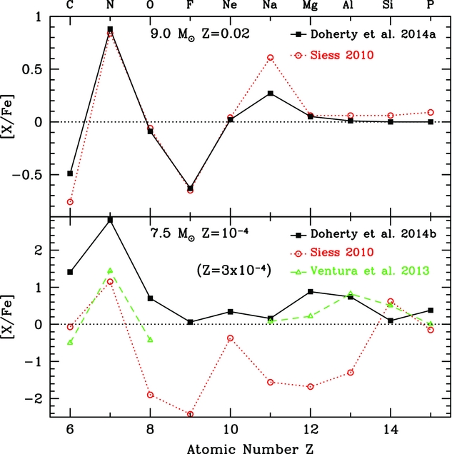
We stress that although agreement between results from different groups at high metallicity is somewhat comforting, the principal test of the validity of our results will come when we can compare against observations, which requires us to positively identify super-AGB stars.
For details of nucleosynthesis in extremely metal-poor (Z ⩽10−5) and primordial super-AGB stars, we refer to the companion review by Gil-Pons et al. (in preparation).
4.3.2. Heavy elements
Due to both the numerical complexities and the time consuming nature of the calculations, currently published heavy element yield predictions of super-AGB stars are limited to a small selection of individual models in Fishlock et al. (Reference Fishlock, Karakas, Lugaro and Yong2014), Shingles et al. (Reference Shingles, Doherty, Karakas, Stancliffe, Lattanzio and Lugaro2015) and Karakas & Lugaro (Reference Karakas and Lugaro2016). There are also calculations for selected species in Karakas et al. (Reference Karakas, García-Hernández and Lugaro2012) and Lugaro et al. (Reference Lugaro2014). In these works, heavy element production is limited to predominantly Rb and in not large quantities. This nucleosynthesis is illustrated by Figure 10 in which we present a new set of yields of heavy elements (via s-process nucleosynthesis) for a range of metallicities Z = 0.02 − 0.001. These calculations are based on the evolutionary models from Doherty et al. (Reference Doherty, Gil-Pons, Lau, Lattanzio and Siess2014a, Reference Doherty, Gil-Pons, Lau, Lattanzio, Siess and Campbell2014b) and use the 324 species nucleosynthetic network detailed in Lugaro et al. (Reference Lugaro2014). These models are chosen as representative of intermediate-mass super-AGB stars and all have very similar core masses (~1.15 M⊙), thermally pulsing durations (~6 × 10⁴ yr), and number of thermal pulses (≈100). As mentioned previously, the high temperature within the helium burning shell during the convective thermal pulses leads to strong activation of the 22Ne neutron source with very high peak neutron densities N n ~1014 cm−3. However, with the very short thermal pulse duration, the integrated neutron exposure τ is not very high, at most ~ 0.04 mbarn−1. This results in a large production of Kr (Z = 36), Rb (Z = 37) and light s-process elements Sr, Y, and Zr (Z = 38, 39, and 40, respectively), and a small synthesis of heavy s-process elements and Pb. The heavy element abundance patterns are similar between models of the different metallicities even with the associated large variation in availability of Fe-seeds. This is due to the low neutron exposure that inhibits formation of substantial amounts of elements past the light s-process peak as well as the small overlap factor between successive thermal pulses which leads to little build up of heavy elements to be subsequently reprocessed. Even with their large number of thermal pulses, heavy element production within super-AGB stars (at least for the moderate metallicities presented here), is reasonably modest, with the yield of no heavier than Fe element exceeding unity in [X/Fe]. This is mostly a consequence of the small mass contained within each convective thermal pulse (~5 × 10⁻⁴ M⊙) and therefore considerable dilution of s-process enriched intershell material within a massive envelope.
Heavy element nucleosynthesis yields for super-AGB stars for a range of metallicities (in [X/Fe]) all scaled to the solar abundances of Asplund et al. (Reference Asplund, Grevesse, Sauval and Scott2009). The breaks in the distribution are for the elements Tc (Z = 43) and Pm (Z = 61) which have no stable isotopes. The shaded regions represent the elements used to represent the three s-process peaks ls, hs, and Pb. The maximum production is for the element Rb (Z = 37).
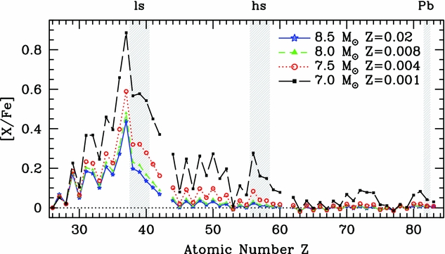
The super-AGB models of Jones et al. (Reference Jones, Ritter, Herwig, Fryer, Pignatari, Bertolli and Paxton2016a) found proton ingestion during TPs where protons from the envelope were making contact with the convective HeB during the thermal pulse. This leads to rapid production of 13C, which then undergoes the 13C(α,n)16O reaction. The neutrons produced during this event are available to then form heavy elements via the intermediate capture process. Jones et al. (Reference Jones, Ritter, Herwig, Fryer, Pignatari, Bertolli and Paxton2016a) estimated the potential i-process heavy element production within super-AGB stars to be of the order of 1–2 dex, comparable to the maximum 1–2.5 dex production from the 22Ne source as estimated by Doherty et al. (Reference Doherty, Gil-Pons, Lau, Lattanzio and Siess2014a, Reference Doherty, Gil-Pons, Lau, Lattanzio, Siess and Campbell2014b).
4.4. Contribution to chemical evolution
Due to a lack of stellar yield calculations, super-AGB stars had long been missing in galactic chemical evolution studies, with this mass range either treated by interpolating between lower-mass AGB stars and massive stars (e.g. Romano et al. Reference Romano, Karakas, Tosi and Matteucci2010; Kobayashi, Karakas, & Umeda Reference Kobayashi, Karakas and Umeda2011), or even neglected entirely. Now, with the recent availability of grids of super-AGB stellar yields (from a variety of research groups and utilising quite different input physics), we are beginning to be able to answer the question of how important are these stars, within a galactic perspective.
In Doherty et al. (Reference Doherty, Gil-Pons, Lau, Lattanzio and Siess2014a), metal-rich super-AGB yields were weighted by a standard IMF and compared to the contribution from lower-mass AGB stars to assess their relative importance. This showed that whilst metal-rich super-AGB stars are large producers of isotopes such as 4He, 13C, 14N, 17O, 22Ne, and 23Na, from a galactic context their contribution is minimal. In Figure 11, we have selected two illustrative isotopes, 7Li and 13C. For 13C, the overall contribution is practically negligible compared to that from the intermediate-mass AGB stars. However, depending on the choice of mass-loss rate, super-AGB stars at high/moderate metallicities may make a contribution to the Galactic inventory of 7Li, 25, 26Mg, and 27Al. Super- (and massive) AGB stars also contribute a non-negligible amount (≈ 10%) to the galactic value of the radioactive isotope 26Al (Siess & Arnould Reference Siess and Arnould2008; Doherty et al. Reference Doherty, Gil-Pons, Lau, Lattanzio and Siess2014a). As mentioned in Section 4.3, the yields of super-AGB stars vary quite considerably between the results from different research groups. This variation is less pronounced at higher metallicities. making predictions from these models reasonably robust.
Stellar yields weighted by the Kroupa, Tout, & Gilmore (Reference Kroupa, Tout and Gilmore1993) IMF, with the shaded regions representing the mass range for super-AGB stars. For masses lower than 6 M⊙ AGB yields are from Karakas (Reference Karakas2010). The error bars on the 8.5 M⊙ Z = 0.02 are mass-loss test cases from Doherty et al. (Reference Doherty, Gil-Pons, Lau, Lattanzio and Siess2014a).
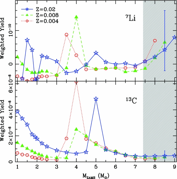
Based on current model predictions, super-AGB stars (at least of mid to high metallicity Z ≳ 0.001) are not expected to make a substantial contribution to the heavy elements in the Galaxy. This is of course dependent on the choice of mass-loss rate, with a larger contribution expected for a slower mass-loss rate. In super-AGB stars, there is considerable dilution of s-process enriched intershell material within the massive envelope. Yet super-AGB stars may still make an important contribution to the light s-process elements, in particular Rb, Sr, and Y in the early Galaxy. Currently, the impact of the possible heavy element (i-process) nucleosynthesis in dredge-out events (Doherty et al. Reference Doherty, Gil-Pons, Siess, Lattanzio and Lau2015; Jones et al. Reference Jones, Ritter, Herwig, Fryer, Pignatari, Bertolli and Paxton2016a) and proton ingestion during thermal pulses (Jones et al. Reference Jones, Ritter, Herwig, Fryer, Pignatari, Bertolli and Paxton2016a) awaits detailed nucleosynthesis calculations.
4.5. Globular cluster abundance anomalies
The ‘abundance anomaly problem’ in globular clusters involves explaining the origin of the unusual compositions present in a substantial fraction (often a majority) of the stars in globular clusters. These patterns are not seen in field stars, and include, for example, He enrichment and anti-correlations in the element pairs C–N, O–Na, and Mg–Al (Carretta et al. Reference Carretta2009a, Reference Carretta, Bragaglia, Gratton and Lucatello2009b; Bragaglia et al. Reference Bragaglia2010). These abundance patterns are characteristic of the results of hot hydrogen burning (Denisenkov & Denisenkova Reference Denisenkov and Denisenkova1990; Prantzos, Charbonnel, & Iliadis Reference Prantzos, Charbonnel and Iliadis2007). Crucially, in the majority of clusters there is no variation, from star to star, in the Fe and heavy (s-process) element abundances (e.g. Yong et al. Reference Yong, Aoki, Lambert and Paulson2006, Reference Yong, Lambert, Paulson and Carney2008). There also seems to be a near constancy in the total C + N + O abundance (e.g. Smith et al. Reference Smith, Shetrone, Bell, Churchill and Briley1996; Ivans et al. Reference Ivans, Sneden, Kraft, Suntzeff, Smith, Langer and Fulbright1999), with some exceptions (e.g. NGC1851, Yong et al. Reference Yong, Grundahl, D’Antona, Karakas, Lattanzio and Norris2009). This would limit the amount of dredged-up material as this contains primary carbon (and its burning products), whereas H burning simply cycles CNO elements among each other, leaving C + N + O constant.
The leading theory to explain these anomalies is that globular clusters are made of multiple generations of stars, with the anomalous stars being formed from the enriched material from a first generation of stars (for a review refer to Gratton, Carretta, & Bragaglia Reference Gratton, Carretta and Bragaglia2012). Many candidates sites have been proposed as the source of the enriching gas such as the following: (super-)AGB stars (Cottrell & Da Costa Reference Cottrell and Da Costa1981; Ventura et al. Reference Ventura, D’Antona, Mazzitelli and Gratton2001; D’Ercole et al. Reference D’Ercole, Vesperini, D’Antona, McMillan and Recchi2008); rapidly rotating massive stars (Decressin et al. Reference Decressin, Meynet, Charbonnel, Prantzos and Ekström2007); massive binary stars (de Mink et al. Reference de Mink, Pols, Langer and Izzard2009); super-massive stars (Denissenkov & Hartwick Reference Denissenkov and Hartwick2014) and novae (Smith & Kraft Reference Smith and Kraft1996; Maccarone & Zurek Reference Maccarone and Zurek2012).
Currently, each of the suspected polluters has problems matching certain observed abundance patterns (Gratton et al. Reference Gratton, Carretta and Bragaglia2012) as well as larger problems such as the mass budget for the different populations and the polluted material (e.g. Bastian & Lardo Reference Bastian and Lardo2015). The entire picture of multiple stellar generations seems incompatible with observations from young massive clusters (the best current day globular cluster analogues) that show a lack of available gas, and no evidence for multiple bursts of star formation (see Bastian Reference Bastian, Charbonnel and Nota2015, and references therein).
Whilst there are problems with the (super-)AGB scenario, as well argued by Renzini et al. (Reference Renzini2015) and D’Antona et al. (Reference D’Antona, Vesperini, D’Ercole, Ventura, Milone, Marino and Tailo2016), using solely nucleosynthetic considerations super-AGB and massive AGBs are perhaps the only barely plausible progenitor candidate remaining. This is based on their ability to (qualitatively) reproduce many of the necessary features, such as high helium content (primarily from SDU) and Li production. They also reach high enough temperatures to activate not only the CNO cycles but also the Ne–Na and Mg–Al chains/cycles.
Observations of Mg–K anti-correlations in the low metallicity globular clusters NGC2419 and NGC2808 (Mucciarelli et al. Reference Mucciarelli, Bellazzini, Ibata, Merle, Chapman, Dalessandro and Sollima2012; Cohen & Kirby Reference Cohen and Kirby2012; Mucciarelli et al. Reference Mucciarelli, Bellazzini, Merle, Plez, Dalessandro and Ibata2015) have been explained as being produced from (very) hot hydrogen burning within the argon–potassium (Ar–K) chain (Ventura et al. Reference Ventura, D’Antona, Di Criscienzo, Carini, D’Ercole and Vesperini2012c). This is shown in Figure 8. Under laboratory conditions the half-life of 37Ar to electron capture is 53 days, whilst at conditions found in super-AGB star envelopes with ρ ~ 10 g cm−3 this half-life is increased to 88 years. Due to this, Iliadis et al. (Reference Iliadis, Karakas, Prantzos, Lattanzio and Doherty2016) argued that the main path to 39K would be via the 36Ar(p,γ)37K(β+ν)37Ar(p,γ)38K(β+ν)38Ar(p,γ)39K channel. Iliadis et al. (Reference Iliadis, Karakas, Prantzos, Lattanzio and Doherty2016) used Monto Carlo nuclear reaction network calculations to identify a temperature and density regime that could explain all the abundance patterns in the cluster NGC2419, in particular the Mg–K anti-correlation. They ruled out the majority of polluter candidates but concluded that super-AGB stars may be a viable solution if the HBB temperatures could be increased slightly, such as results from the use of the FST theory of convection. In fact, Iliadis et al. (Reference Iliadis, Karakas, Prantzos, Lattanzio and Doherty2016) identified that novae also may reach the correct temperature/density conditions, but without any detailed nova models available for low metallicity this needs further exploration, and remains quite speculative.
Probably the major nucleosynthetic problem with the (super-)AGB scenario currently is the fine balance of conditions required to produce 23Na instead of destroying it. To achieve the high depletion of O (and Mg) that is observed, the duration of the TP-(S)AGB phase needs to be quite extended. However this leads also to destruction of 23Na, whereas the stars depleted in O are enhanced in 23Na. A remedy to this problem could come from a decrease in the reaction rate of 23Na(p,α)20Ne destruction channel by a factor of 2–5 (Ventura & D’Antona Reference Ventura and D’Antona2006). We note however that this value is outside the current uncertainties. An experimental re-evaluation of this reaction rate is clearly justified.
Another nucleosynthetic obstacle for the (super-)AGB star scenario (and all other polluter candidates) is the production of too much 4He to match the observed spread in the majority of clusters (Bastian, Cabrera-Ziri, & Salaris Reference Bastian, Cabrera-Ziri and Salaris2015). Helium in massive AGB and super-AGB stars is produced primarily from SDU, with a smaller contribution from HBB. These processes are quite independent, so there is some potential scope to modify the 4He production.
Another important and often overlooked point is the impact of rotation on the surface composition. Decressin et al. (Reference Decressin, Charbonnel, Siess, Palacios, Meynet and Georgy2009) showed that rotation in intermediate-mass stars may act like deep (corrosive) SDU and increase the surface in carbon (and total metallicity), which would make (super-)AGB stars unviable polluter candidates.
As we saw in Section 4.3, the predictions of super-AGB star nucleosynthesis at low metallicity (applicable to the majority of globular clusters) vary widely between different research groups. For super-AGB star models to match as the polluter they must fit rather strict evolutionary constraints. These are no, or very inefficient TDU; very advanced HBB, driven either by more efficient convective mixing (e.g. through use of FST), or standard mixing-length theory with increased mixing-length parameter α; a relatively slow mass-loss rate. In addition, as discussed in Pumo, D’Antona, & Ventura (Reference Pumo, D’Antona and Ventura2008), the most massive super-AGB stars, which undergo dredge-out events, must all end their lives as EC-SNe to avoid polluting the cluster with C enriched material.
However, if (super-)AGB stars are indeed the source of the material from which the later generation(s) formed this would prove invaluable to constraining theoretical modelling of this class of star.
4.6. Dust production
AGB and super-AGB stars make substantial contributions to the galactic dust inventory (e.g. Gehrz Reference Gehrz, Allamandola and Tielens1989; Matsuura et al. Reference Matsuura2009; Schneider et al. Reference Schneider, Valiante, Ventura, dell’Agli, Di Criscienzo, Hirashita and Kemper2014). The type of dust formed during the (super-)AGB phase is determined by the surface composition of the star, primarily the C/O ratio, and is classified into two main groups: either carbon-rich or oxygen-rich. As seen in the previous sections, due to HBB the surface composition in super-AGB stars is typically C/O < 1 for the majority of the TP-SAGB phase. Thus, super-AGB stars are expected to produce silicates (olivine, pyroxene, and quartz), alumina dust and no or very little carbon dust (e.g. Ventura et al. Reference Ventura2012a). Dust yields have now been calculated for super-AGB stars over the wide range of metallicities Z = 0.001 − 0.018 (Ventura et al. Reference Ventura2012a, Reference Ventura2012b, Reference Ventura, Dell’Agli, Schneider, Di Criscienzo, Rossi, La Franca, Gallerani and Valiante2014; Dell’Agli et al. Reference Dell’Agli, García-Hernández, Rossi, Ventura, Criscienzo and Schneider2017).
The amount of dust generated depends critically on the density in the stellar outflow, with more rapid mass loss leading to higher density and greater dust production. This results in dust mass yields (and silicate dust grain sizes), which are correlated with initial mass. The most massive super-AGB stars produce ~ 10−3 to 10−2 M⊙ with grain size ≲0.15 μm (Dell’Agli et al. Reference Dell’Agli, García-Hernández, Rossi, Ventura, Criscienzo and Schneider2017). Models of O-rich super-AGB stars from Ventura et al. (Reference Ventura2012b) find the amount of dust production is strongly metallicity dependent, with decreasing dust yields at lower metallicity. This is due to the reduced availability of the key elements Si, Al, Fe, and O at lower metallicity, as well as the far lower O abundance due to the more efficient HBB at low metallicity. Since these elements are not produced in substantial amounts within the stars themselves, dust formation is expected to be inhibited. At the metallicity of Z = 3 × 10⁻⁴ Di Criscienzo et al. (Reference Di Criscienzo2013) found the Si abundance was too low for non-negligible silicate production. They suggested a metallicity threshold of Z = 0.001 as the limit for silicate production for super-AGB stars. As yet, there are no dust yield calculations from models that have undergone dredge-out and become C-rich at the start of the super-AGB phase, nor of super-AGB star models that have become carbon rich due to either TDU or very efficient O destruction. These models would result in substantially different dust chemistry and warrant exploration.
5 DISCUSSION AND CONCLUSIONS
Here, we discuss some of the observational probes and studies that can be, and are being, used to aid in the understanding of the evolution of stars that bridge the low/high mass divide.
5.1. Observational constraints
As mentioned in the introduction, a fundamental problem is that there are at present no definite detections of super-AGB stars. Their very rapid mass-loss rates are expected to produce dust enshrouded OH/IR stars that are more luminous than their lower-mass AGB star counterparts. However, models that undergo more efficient convective mixing (e.g. through using the FST theory of convection or a larger mixing-length within the MLT formulation) will attain higher luminosities, making clear identification between a massive AGB and a super-AGB star practically impossible. Furthermore, from a nucleosynthetic point of view a low-mass super-AGB star and a massive AGB star are expected to produce very similar element distributions, in particular for the heavier than Fe elements. At present abundance determinations in massive (potentially super-)AGB stars are limited to a small sample of stars in the Galaxy and Magellanic clouds (García-Hernández et al. Reference García-Hernández, García-Lario, Plez, D’Antona, Manchado and Trigo-Rodríguez2006, Reference García-Hernández, García-Lario, Plez, Manchado, D’Antona, Lub and Habing2007, Reference García-Hernández2009). These stars are found to be Rb-rich, which is suggestive that they have undergone TDU events. Determining the exact amount of enrichment is problematic as it has been shown that accounting for an extended circumstellar envelope can substantially modify the abundance determinations in this class of star (Zamora et al. Reference Zamora, García-Hernández, Plez and Manchado2014). Super-AGB stars may also be identified in the large infrared surveys of Magellanic clouds (e.g. Kraemer et al. Reference Kraemer, Sloan, Wood, Jones and Egan2017), or in young stellar clusters.
Super-AGB stars also share the same stellar luminosities and surface temperatures as the slightly more massive red super-giants. Hence, a careful analysis of red super-giant surveys may yield super-AGB star candidates. One such object is the star HV2112 (Levesque et al. Reference Levesque, Massey, Żytkow and Morrell2014), which has been suggested potentially as a super-AGB star, or even a Thorne–Żytkow object (Tout et al. Reference Tout, Żytkow, Church, Lau, Doherty and Izzard2014). Stellar variability may be a key to distinguish between red super-giants and super-AGB stars with super-giants expected to have lower amplitude pulsations, with maximum variations of about 0.5 mag (Wood, Bessell, & Fox Reference Wood, Bessell and Fox1983; Groenewegen et al. Reference Groenewegen, Sloan, Soszyński and Petersen2009).
5.1.1. Low mass channel
Planetary nebula abundances may be used as probes of the resultant nucleosynthesis in super-AGB stars (e.g. Ventura et al. Reference Ventura, Stanghellini, Dell’Agli, García-Hernández and Criscienzo2015, Reference Ventura, Stanghellini, Di Criscienzo, García-Hernández and Dell’Agli2016; García-Hernández et al. Reference García-Hernández, Ventura, Delgado-Inglada, Dell’Agli, Di Criscienzo and Yagüe2016). However, as these stars represent only a relatively scarce (and short-lived) mass range we expect only a small number of such planetary nebulae.
White dwarfs can be used to explore the evolutionary properties of super-AGB stars in a variety of ways, such as WD mass distributions/population studies, initial-final mass relations and analysis of individual massive WDs.
We note that observations of massive (i.e. exceeding 0.8M⊙) and ultra-massive (exceeding 1.1M⊙) white dwarfs are particularly difficult due to their relative scarcity, inherently low luminosity due to their more compact nature, as well as more rapid cooling (Althaus et al. Reference Althaus, García-Berro, Isern, Córsico and Rohrmann2007). Works by Williams, Bolte, & Koester (Reference Williams, Bolte and Koester2009) and Cummings et al. (Reference Cummings, Kalirai, Tremblay and Ramirez-Ruiz2016a, Reference Cummings, Kalirai, Tremblay, Ramirez-Ruiz and Bergeron2016b) have derived semi-empirical initial-final mass relations with particular focus on massive and ultra-massive WDs using observations from young open clusters. However, the procedure to derive an initial-final mass relation is quite involved and is affected by quite a range of uncertainties. Firstly, the WD effective temperature and gravity are determined from observations and the mass is then determined from a mass to radius relation. Next, the cluster age is found from isochrone fitting with this procedure reliant on stellar evolution models with their inherent uncertainties. The initial mass of the WD is determined by estimating the cooling time, which is dependent on composition e.g. CO (Salaris et al. Reference Salaris, Dominguez, Garcia-Berro, Hernanz, Isern and Mochkovitch1997, Reference Salaris, Cassisi, Pietrinferni, Kowalski and Isern2010) or ONe (Althaus et al. Reference Althaus, García-Berro, Isern, Córsico and Rohrmann2007), and then subtracting this from the cluster age to find the stellar lifetime. Lastly, this duration is compared to theoretical stellar models to derive the initial mass. With the stellar lifetimes of super-AGB stars quite short (~20–60 Myr) and dependent on rotational mixing and overshoot among other effects, the determination of an initial mass for a ultra-massive WD will be hampered by large uncertainties. Hence, this method seems unlikely to be able to accurately determine a reliable upper mass limit for WD formation. Based on current estimates of the initial-final mass relation the maximum mass for a WD progenitor is estimated to be in range ~7.5 to 10 M⊙ or more (Salaris et al. Reference Salaris, Serenelli, Weiss and Miller Bertolami2009; Williams et al. Reference Williams, Bolte and Koester2009; Cummings et al. Reference Cummings, Kalirai, Tremblay and Ramirez-Ruiz2016a).
Theoretical calculations from single or binary intermediate-mass stars predict a veritable zoo of massive WDs including: CO, CO–Ne, ONe, Si, and ONeFe WDs. Observationally distinguishing between these may prove to be practically impossible. Two ultra-massive (~ 1.1M⊙) O-rich (Gänsicke et al. Reference Gänsicke, Koester, Girven, Marsh and Steeghs2010) WDs have been observed.Footnote 10 In principle differentiating between the CO or ONe core composition of a massive WD can be accomplished from asteroseismology of pulsating WDs (Córsico et al. Reference Córsico, García-Berro, Althaus and Isern2004). Another way to probe WD interiors comes from either classical or neon novae, which are hosted on CO and ONe WDs (Jose & Hernanz Reference Jose and Hernanz1998; Wanajo et al. Reference Wanajo, Hashimoto and Nomoto1999; Gil-Pons et al. Reference Gil-Pons, García-Berro, José, Hernanz and Truran2003b; Downen et al. Reference Downen, Iliadis, José and Starrfield2013), respectively; however, these observations will most likely probe only the outer layers.
5.1.2. High mass channel
There is the potential to learn about the final fates of intermediate-mass stars through studies of SNe and their remnants. The most common approach is to identify particular events and make direct comparison between models and observed properties such as chemistry, mass-loss history, light curves, etc. The overall SN rate may be used to estimate the minimum mass for a SN. In addition, it may also be possible to use predicted nucleosynthetic properties to determine the frequency of certain types of SN events.
Have we already seen the death throes of a supernova from a super-AGB star? With their H rich envelopes, single super-AGB stars are expected to explode as Type II SN. EC-SNe are expected to have lower explosion energies of ≈1050 erg and very small Ni masses ~1–3 × 10⁻³ M⊙ (Kitaura et al. Reference Kitaura, Janka and Hillebrandt2006) compared to their more-massive FeCC-SN counterparts (≈ 1051 erg, ~5 × 10⁻² M⊙). The envelopes of super-AGB star progenitors of EC-SNe may be either C-rich or O-rich prior to explosion, with dredge-out events being able to form carbon stars, albeit only for a short time before efficient HBB would burn this C to N resulting in C/O < 1.
Owing to the substantial difference in envelope configurations and mass-loss histories that are possible prior to an EC-SN, there is potential for a wide variation in observable events. Hence, many different classes of SNe have been suggested to originate from EC-SNe:
-
(i) the sub-luminous class of II-P including SN2003gd, SN2005cs, SN2008bk, SN2009md (Kitaura et al. Reference Kitaura, Janka and Hillebrandt2006)
-
(ii) the so-called ‘supernova impostors’ of SN2008S (Botticella et al. Reference Botticella2009; Pumo et al. Reference Pumo2009), SN2008ha (Foley et al. Reference Foley2009; Valenti et al. Reference Valenti2009), and NGC300-OT (Prieto et al. Reference Prieto, Sellgren, Thompson and Kochanek2009);
-
(iii) a subset of the IIn-P class which includes SN1054 (the Crab nebula progenitor; Davidson et al. Reference Davidson1982; Nomoto et al. Reference Nomoto, Sugimoto, Sparks, Fesen, Gull and Miyaji1982; Tominaga, Blinnikov, & Nomoto Reference Tominaga, Blinnikov and Nomoto2013), SN1994W, SN2009kn, and SN2011ht (Smith Reference Smith2013)
Due to their low explosion energy, it had been assumed that EC-SNe may also be of low luminosity. Hence, they have been associated with the sub-luminous members of the II-P SN category (e.g. Kitaura et al. Reference Kitaura, Janka and Hillebrandt2006). This association has fallen out of favour recently as a result of modelling of EC-SN lightcurves, which found them to be as bright as typical Type II-P SNe (Tominaga et al. Reference Tominaga, Blinnikov and Nomoto2013; Moriya et al. Reference Moriya, Tominaga, Langer, Nomoto, Blinnikov and Sorokina2014) due to their large progenitor radius and small envelope mass. Another problem for this scenario comes from archival pre-SN proprieties of SN 2005cs. These showed that the progenitor had a luminosity far too low to be consistent with models in the post-SDU/dredge-out phase of super-AGB evolution (Eldridge, Mattila, & Smartt Reference Eldridge, Mattila and Smartt2007). Probably the most accepted model is that these sub-luminous SNe have slightly more massive progenitors ~10–15 M⊙ (Spiro et al. Reference Spiro2014).
Whilst there are some very promising candidate EC-SN, in particular SN1054 and SN2008S, as yet there has been no definitive confirmed super-AGB EC-SN events.
Based on observations of Type II-P SNe, which also had pre-SN progenitor imaging, the review by Smartt (Reference Smartt2009) estimated the lower initial mass for CC-SN explosions to be 8.5+1 −1.5 M⊙. However, with an increased data set, this value was revised to 9.5+0.5 −2 M⊙ or 10+0.5 −1 M⊙ depending on choice of stellar models (Smartt Reference Smartt2015). These values for M n are in reasonable agreement with the theoretical stellar evolutionary calculations discussed in Section 3.1, which take into account a moderate amount of overshooting. Under the assumption of the minimum initial mass for a CC-SN to be 8 M⊙, the recent SUDARE supernova survey (Botticella et al. Reference Botticella2017) found the expected CC-SN rate to be higher than the value deduced from observations by about a factor of 2. A possible remedy to this discrepancy is if the minimum mass for a CC-SN was increased to 10 M⊙.
From an explosive nucleosynthesis perspective super-AGB stars that undergo an EC-SN may produce a wide variety of elements from Zn to Zr (Wanajo et al. Reference Wanajo, Janka and Müller2011), and isotopes 48Ca and 60Fe (Wanajo, Janka, & Müller Reference Wanajo, Janka and Müller2013a, Reference Wanajo, Janka and Müller2013b). Based on their calculations of 86Kr, Wanajo et al. (Reference Wanajo, Janka and Müller2011) suggested the frequency of EC-SNe relative to all CC-SNe must be ~4%, assuming that the vast majority of this isotope in the solar system originates from EC-SNe. However, Wanajo et al. (Reference Wanajo, Müller, Janka and Heger2017) found that the nucleosynthesis from core collapse models of either O–Ne–Mg cores or the lowest-mass Fe cores (dubbed ‘EC-SNe like’) is almost identical. Owing to this inability to distinguish resultant yields they suggest the EC-SN and low-mass FeCC-SN channel should be about 0.5–1 M⊙ wide in initial mass, if these events are the main source of elements Zn to Zr in the Galaxy.
Recent determinations of the neutron star mass distribution have suggested that it may be bimodal (Schwab, Podsiadlowski, & Rappaport Reference Schwab, Podsiadlowski and Rappaport2010; Knigge, Coe, & Podsiadlowski Reference Knigge, Coe and Podsiadlowski2011; Valentim, Rangel, & Horvath Reference Valentim, Rangel and Horvath2011), with the lower mass peak suspected to arise from EC-SNe (van den Heuvel Reference van den Heuvel, Schoenfelder, Lichti and Winkler2004; Podsiadlowski et al. Reference Podsiadlowski, Langer, Poelarends, Rappaport, Heger and Pfahl2004). Due to the steep density gradient at the core edge it is expected that EC-SNe result in neutron star masses very close to that of the original ONeMg core and with relatively small kick velocities (Podsiadlowski et al. Reference Podsiadlowski, Dewi, Lesaffre, Miller, Newton and Stone2005; Radice et al. Reference Radice, Burrows, Vartanyan, Skinner and Dolence2017). However, recent low-mass FeCC-SN and EC-SN progenitor models show smaller differences in the density gradients than in previous calculations (e.g. see Figure 1 in Müller Reference Müller2016) and due to this have far more similar explosion properties than in previous works. Owing to their similarity in explosion properties, the resulting neutron star masses may not be as clearly distinguishable as was thought, making it harder to separate neutron stars from the lowest mass FeCC-SNe and EC-SNe.
As described in Section 3.3, binary evolution opens new formation channels for EC-SNe. In the scenario that involves the merger of two WDs, the signature is expected to be that of a SN of Type Ib (Nomoto & Hashimoto Reference Nomoto and Hashimoto1987). If we consider a CV-like configuration of an accreting ONe WD, the explosion properties depend on the mass-transfer rate. If accretion is slow, helium will build up at the surface of the WD and eventually ignite off-center. The detonation will then produce observational signatures similar to those of a SNIa (Marquardt et al. Reference Marquardt, Sim, Ruiter, Seitenzahl, Ohlmann, Kromer, Pakmor and Röpke2015). In the other class of models where the progenitor loses its H-rich envelope and becomes a He star, the EC-SN explosion would be observed as a SNIb or Ic depending of the mass and composition of the envelope surrounding the collapsing ONe core (Tauris et al. Reference Tauris, Langer and Podsiadlowski2015). According to Moriya & Eldridge (Reference Moriya and Eldridge2016), the explosion of stripped-envelope EC-SNe could give rise to fast evolving transients and the newly-formed neutron star would have a low kick velocity.
5.2. Critical uncertainties
5.2.1. Mass loss
The very large uncertainty in the mass-loss rates for super-AGB stars, particularly at low metallicity, is a major impediment to determining the final fates of this class of star. Whilst there are observational studies examining the impact of metallicity on the mass-loss rates of AGB and red super-giant stars (e.g. Matsuura et al. Reference Matsuura2016; Goldman et al. Reference Goldman2017), these works can only probe the relatively metal rich populations, because the low metallicity super-AGB stars are long since dead. However, there are valiant efforts underway in theoretical modelling of AGB star atmospheres and circumstellar envelopes to derive a predictive theory of mass loss for (super-)AGB stars (see Höfner Reference Höfner2016 and references therein). In addition to the importance of determining the ‘standard’ mass loss from super-AGB stars, there may also be mass expulsions from either the Fe-peak instability (Lau et al. Reference Lau, Gil-Pons, Doherty and Lattanzio2012) or convective-reactive H-ingestion episodes (Jones et al. Reference Jones, Ritter, Herwig, Fryer, Pignatari, Bertolli and Paxton2016a). Both of these phenomena may have a substantial impact on the frequency of EC-SNe, as well as potentially modify super-AGB nucleosynthesis. They warrant further examination. Based on observations of evolved massive AGB stars de Vries et al. (Reference de Vries, Blommaert, Waters, Waelkens, Min, Lombaert and Van Winckel2014, Reference de Vries, Maaskant, Min, Lombaert, Waters and Blommaert2015) have suggested the need for a ‘hyper’-wind of 10−3–10−2 M⊙ yr−1 to account for the very short superwind duration and lack of extended structure (Cox et al. Reference Cox2012). Could this hyperwind be as a result of an Fe peak instability?
5.2.2. Convection
Our current theory of convection, in particular the treatment of convective boundaries, lies at the heart of the majority of the uncertainties in this mass range. Arguably, the most important factor that effects the mass boundaries M up and M mas is the treatment of convective borders, in particular during core He burning. Multi-dimensional hydrodynamical simulations of convection are key to understanding this mass range. A new theory of convection, such as the 321D theory under development (Arnett et al. Reference Arnett, Meakin, Viallet, Campbell, Lattanzio and Mocák2015; Campbell et al. Reference Campbell2016), would help to constrain the WD/SN boundary.
Is convective boundary mixing efficient enough to stall C, and/or Ne burning i.e. do CO–Ne WDs or failed massive stars exist? While the study of Lecoanet et al. (Reference Lecoanet2016) suggested the C-burning would most likely not be stalled by CBM, the results from C burning flame propagation cannot simply be applied to that of neon–oxygen burning flames to rule out the formation of failed massive stars. This is due to the structure between C and Ne flames being quite different with Ne burning flames far thinner and faster moving (e.g. Timmes et al. Reference Timmes, Woosley and Taam1994). Multi-dimensional calculations of Ne flames are crucial to determine if failed massive stars exist.
What is the impact of convective boundary mixing on the occurrence and efficiency of third dredge-up? Are super-AGB stars the site of the i-process heavy element production from during proton ingestion TPs (Jones et al. Reference Jones, Ritter, Herwig, Fryer, Pignatari, Bertolli and Paxton2016a)?
5.3. Future research topics
There are a number of investigations that could be done in the near future, and which would dramatically advance this field. We list a selection of these here:
-
• an analysis of red super-giant surveys to possibly identify super-AGB stars;
-
• further analysis of convective-reactive H-ingestion events, to determine their implications for super-AGB stars;
-
• examine the conditions for termination of the super-AGB phase, (in particular the Fe opacity peak instability); this will require hydrodynamical models but could yield significant advances in our understanding of the masses and progenitors of various SNe;
-
• hydrodynamical multi-dimensional flame propagation calculations, especially for the Ne flame;
-
• re-evaluation/measurement of the critical nuclear reaction rates: 23Na + p, 12C+12C;
-
• details of dust production from carbon rich super-AGB and massive AGB stars;
-
• proton ingestion and the resulting i-process neutron captures; this may have implications well beyond super-AGB stars;
-
• further numerical modelling of EC-SNe and the lowest-mass Fe-CC-SNe to enable predictions of observation properties such as lightcurves, nucleosynthetic signatures, etc., which may help to distinguish between these two types of progenitors;
-
• binary star evolutionary calculations over a larger parameter space to further constrain the impact of the binary channnel on formation of EC-SNe.
5.4. Conclusion
The last decade has seen real advances in the study of the lives and deaths of super-AGB stars. There are now fully detailed interior stellar evolutionary models along the entire TP-SAGB for a wide range of metallicities from Z = 0.04 to Z = 10−5 (see companion review by Gil-Pons et al. 2017). Furthermore super-AGB star nucleosynthesis predictions for both light and heavy elements are now available for some compositions, and the composition range is being extended all the time. The first detailed dust yields are also now available.
The study of EC-SNe has flourished in recent years. The production of a new generation of single star EC-SN progenitor models is an important update on the previous models from the early 1980s. There are now detailed single and multi-dimensional simulations of EC-SNe (and EC-SN like) explosions as well as detailed nucleosynthetic calculations from EC-SNe. In addition, recent works have calculated synthetic light-curves of EC-SNe within super-AGB star envelopes. There have also been important advances in the role of binary stars in producing EC-SNe.
All of these above results have produced predictions that can be, and are being, tested against observation to further constrain these stars on the low/high mass star boundary.
Nevertheless, some of the most important questions remain. For example, recent multi-dimensional simulations of O-deflagration in ONe cores have reopened the debate on the final fate of an EC-SN and whether they explode by oxygen deflagration, or collapse by electron capture to form a neutron star.
Finally, we have identified areas that need attention, which may help us finally answer some of these important questions.
ACKNOWLEDGEMENTS
This work was supported in part by the National Science Foundation under Grant no. PHY-1430152 (JINA Center for the Evolution of the Elements). This work was supported by Spanish MINECO grant AYA2015-71091-P. CD acknowledges support from the Lendulet-2014 Programme of the Hungarian Academy of Sciences. CD would like to thank S.W Campbell, S. Jones, and J. Cummings for interesting discussions. LS is a senior FNRS researcher.