





1. Introduction
When countries import products from abroad, they also import ‘virtual water’, defined as the water embedded in traded products (Allan, Reference Allan1998, Reference Allan2003). Virtual water flows describe how nations rely on water resources in other countries to meet domestic consumption needs (Hoekstra & Mekonnen, Reference Hoekstra and Mekonnen2012). This concept links localized basin-level water demand to transboundary activities and is thus critical for global water resource management (Hoff, Reference Hoff2013; Liu et al., Reference Liu, Hull, Batistella, DeFries, Dietz, Fu, Zhu, Izaurralde, Lambin, Li, Martinelli, McConnell, Moran, Naylor, Ouyang, Polenske, Reenberg, de Miranda Rocha, Simmons and Zhu2013; Vörösmarty et al., Reference Vörösmarty, Hoekstra, Bunn, Conway and Gupta2015). Virtual water flows account for 20% of global water consumption (Hoekstra & Mekonnen, Reference Hoekstra and Mekonnen2012), including green (the consumptive use of precipitation embodied in international trade) and blue virtual water flows (the consumptive use of surface water and groundwater embodied in international trade). When virtual water flows originate from water-scarce regions, they raise sustainability concerns (Hoekstra, Reference Hoekstra2020; Vörösmarty et al., Reference Vörösmarty, Hoekstra, Bunn, Conway and Gupta2015). About 30–50% of virtual water flows originate in physically or economically water-scarce regions (Lenzen et al., Reference Lenzen, Moran, Bhaduri, Kanemoto, Bekchanov, Geschke and Foran2013; Mekonnen & Hoekstra Reference Mekonnen and Hoekstra2020; Rosa et al., Reference Rosa, Chiarelli, Tu, Rulli and D'Odorico2019; Taherzadeh et al., Reference Taherzadeh, Bithell and Richards2021; Vallino et al., Reference Vallino, Ridolfi and Laio2020, Reference Vallino, Ridolfi and Laio2021), which calls for further action to manage virtual water flows.
Understanding the characteristics of the stakeholders involved in virtual water flows is essential for designing effective interventions. This means that not only should we understand the quantity of virtual water flows, but also from whom (farmers and producers), via whom (traders and distributors), and to whom (retailers and consumers) the virtual water is traded internationally. Since around 85% of the international green/blue virtual water flows are crop-related (Hoekstra & Mekonnen, Reference Hoekstra and Mekonnen2012), most studies focus on the agricultural system. Current studies have shown that large multinational agri-food corporations have significant impacts on existing virtual water flows (Baronchelli et al., Reference Baronchelli, Vallino, Dalmazzone, Ridolfi and Laio2024; De Petrillo et al., Reference De Petrillo, Tuninetti, Ridolfi and Laio2023; Sojamo et al., Reference Sojamo, Keulertz, Warner and Allan2012). A single large corporation may trade more virtual water than a major importing country, particularly in cash-crop-related virtual water flows (Baronchelli et al., Reference Baronchelli, Vallino, Dalmazzone, Ridolfi and Laio2024; De Petrillo et al., Reference De Petrillo, Tuninetti, Ridolfi and Laio2023).
The role of farmers in virtual water flows, who directly consume water and supply crops to agri-food corporations, remains poorly understood (Hoekstra et al., Reference Hoekstra, Chapagain, Mekonnen and Aldaya2011; Sun et al., Reference Sun, Tukker and Behrens2019). Small-scale agriculture, which contributes substantially to food security (Ricciardi et al., Reference Ricciardi, Ramankutty, Mehrabi, Jarvis and Chookolingo2018a; Taherzadeh et al., Reference Taherzadeh, Cai and Mogollón2026), has distinguishing characteristics compared to large-scale agriculture. For example, small-scale agriculture generally has different crop structures than large-scale agriculture (Herrero et al., Reference Herrero, Thornton, Power, Bogard, Remans, Fritz, Havlík, Nelson, See, Waha, Watson, West, Samberg, van de Steeg, Stephenson, van Wijk and Havlík2017; Ricciardi et al., Reference Ricciardi, Ramankutty, Mehrabi, Jarvis and Chookolingo2018a). Small-scale agriculture is largely located in water-scarce regions, but uses less irrigation compared with large-scale agriculture (Ricciardi et al., Reference Ricciardi, Wane, Sidhu, Godde, Solomon, McCullough, Mehrabi, Porciello, Jain, Randall and Mehrabi2020; Su et al., Reference Su, Willaarts, Luna-Gonzalez, Krol and Hogeboom2022) and might be inefficient in terms of green water use because of low agricultural input (Su et al., Reference Su, Foster, Hogeboom, Luna-Gonzalez, Mialyk, Willaarts and Krol2025b). Consequently, small-scale farming might play a different role in international trade and virtual water flows than large-scale agriculture (Giller et al., Reference Giller, Delaune, Silva, Descheemaeker, van de Ven, Schut, van Ittersum, Hammond, Hochman, Taulya, Chikowo, Narayanan, Kishore, Bresciani, Teixeira, Andersson and van Ittersum2021). Failing to distinguish the farmers behind virtual water flows may undermine the design of effective water and food security policies (Trottier & Perrier, Reference Trottier and Perrier2017).
Distinguishing between small-scale and large-scale agriculture in global virtual water flows poses methodological challenges. Most international virtual water flow studies focus on the national level. Distinguishing between small-scale and large-scale agriculture requires subnational farm-size-specific production, water consumption, and export information for each crop, which is not always readily available. Though a few studies have estimated farm-size-specific crop production through the allocation of national data (Herrero et al., Reference Herrero, Thornton, Power, Bogard, Remans, Fritz, Havlík, Nelson, See, Waha, Watson, West, Samberg, van de Steeg, Stephenson, van Wijk and Havlík2017; Ricciardi et al., Reference Ricciardi, Ramankutty, Mehrabi, Jarvis and Chookolingo2018b), to our best knowledge, only a recent dataset developed by Su et al. (Reference Su, Foster, Hogeboom, Luna-Gonzalez, Mialyk, Willaarts and Krol2025b) using a gridded crop model provides consistent farm-size-specific production and water consumption data. It covers 171 crops in 55 countries for the period 2008–2012, where the farm-size-specific harvested area is from the subnational agricultural census (Su et al., Reference Su, Willaarts, Luna-Gonzalez, Krol and Hogeboom2022). Compared to crop production and water consumption, subnational export data is even more scarce. Instead of collecting subnational data, it can be estimated by combining various datasets and making certain assumptions, for example, allocating exports based on production (Sun et al., Reference Sun, Tukker and Behrens2019).
In this study, we estimate the contributions of small-scale and large-scale farming to crop production involved in trade and virtual water flows (export-based) for 55 countries, using the baseline 2008–2012 due to data availability. We combined multiregional input–output (MRIO) databases, food and agriculture biomass input–output (FABIO, v1.2; Bruckner et al., Reference Bruckner, Wood, Moran, Kuschnig, Wieland, Maus and Borner2019), and global resource input–output assessment (GLORIA, v059; Lenzen et al., Reference Lenzen, Geschke, West, Fry, Malik, Giljum, Schandl, Piñero, Lutter, Wiedmann, Li, Sevenster, Potočnik, Teixeira, Van Voore, Nansai and Schandl2022) to obtain the national crop production involved in trade at high sectoral resolution, and farm-size-specific crop production and water consumption data (Su et al., Reference Su, Foster, Hogeboom, Luna-Gonzalez, Mialyk, Willaarts and Krol2025b). We allocated the national crop production involved in trade to small-scale and large-scale agriculture based on two assumptions: a production-based assumption (export proportional to production) (Sun et al., Reference Sun, Tukker and Behrens2019) and a farming system-based assumption (export proportional to the production of irrigated and high-input farming systems) (Hoang et al., Reference Hoang, Taherzadeh, Ohashi, Yonekura, Nishijima, Yamabe, Kanemoto, Matsuda, Moran and Kanemoto2023). Based on the above datasets and models, we estimate the contribution of small-scale and large-scale agriculture to the crop production involved in trade, green and blue virtual water export, and the associated sectors that drive them. Here, crop production involved in trade refers to the crop traded, directly or indirectly. The latter means the crop is used as input for exported products. We identify the crops in which small-scale agriculture makes a significant contribution to trade. Furthermore, we reveal the different roles of small-scale and large-scale agriculture in blue and green virtual water flows.
2. Method
We first used the MRIO databases, FABIO (v1.2; Bruckner et al., Reference Bruckner, Wood, Moran, Kuschnig, Wieland, Maus and Borner2019), and GLORIA (v059; Lenzen et al., Reference Lenzen, Geschke, West, Fry, Malik, Giljum, Schandl, Piñero, Lutter, Wiedmann, Li, Sevenster, Potočnik, Teixeira, Van Voore, Nansai and Schandl2022) to estimate the crop production involved in international trade for each crop at the national level. Then, we allocated the crop production involved in trade to small-scale and large-scale agriculture based on their production (production-based assumption) or farming systems (farming system-based assumption). Here, crop production involved in international trade refers not only to the crop production traded directly but also to that traded indirectly, where a crop is used as an input for an exported product. MRIO describes the inputs and outputs of each sector and trade among all the countries. Since the crop production differentiating small-scale and large-scale agriculture by Su et al. (Reference Su, Foster, Hogeboom, Luna-Gonzalez, Mialyk, Willaarts and Krol2025b) is available for 55 countries for the period of 2008–2012, with the main purpose of establishing the baseline estimates, the virtual water flow analysis focuses on the same geographic and temporal scope. These 55 countries are representative across continents and collectively account for more than half of the global cropland.
2.1. Crop production involved in international trade
To describe crop-related international trade with high sector-level detail and less uncertainty, we leveraged a physical MRIO designed for food and agriculture, FABIO (v1.2; Bruckner et al., Reference Bruckner, Wood, Moran, Kuschnig, Wieland, Maus and Borner2019). FABIO covers 192 global countries/areas and 123 agricultural sectors (61 crop sectors). Because FABIO does not track the nonfood uses of crops along the supply chain, we linked it to the GLORIA (v059) MRIO model (Lenzen et al., Reference Lenzen, Geschke, West, Fry, Malik, Giljum, Schandl, Piñero, Lutter, Wiedmann, Li, Sevenster, Potočnik, Teixeira, Van Voore, Nansai and Schandl2022) for further traceability of virtual water flows within the wider resource economy. GLORIA represents the monetary flow of 120 sectors within and between 160 countries and four aggregated regions, including 36 agricultural and 84 nonagricultural sectors.
We connected FABIO and GLORIA using a linking table. To construct the linking table  ${Z_{{\text{link}}}}$, for each region r, we have
 \begin{equation}\begin{array}{*{20}{c}}
{{T^r} = \phi V_{{\text{GLORIA}}}^r\circ \Theta },
\end{array}\end{equation}
\begin{equation}\begin{array}{*{20}{c}}
{{T^r} = \phi V_{{\text{GLORIA}}}^r\circ \Theta },
\end{array}\end{equation}where  $\phi $ is the supply filter matrix defining the GLORIA sectors supplying the FABIO product; $\Theta $ is the use filter matrix defining the potential sectors in GLORIA using the FABIO product; $^\circ $ is the Hadamard product. $V_{{\text{GLORIA}}}^{\text{r}}$ is an aggregation of the GLORIA transaction matrix ${Z_{{\text{GLORIA}}}}$. It first selects the corresponding columns for regions r in ${Z_{{\text{GLORIA}}}}$ and then enumerate along the rows over regions for each sector. ${T^r}$ was further divided by its row sums, resulting $T_{{\text{share}}}^r$. Then for region r, we have
 \begin{equation}\begin{array}{*{20}{c}}
{Z_{{\text{link}}}^r = \left( {\begin{array}{*{20}{c}}
{T_{{\text{share}}}^r} \\
\vdots \\
{T_{{\text{share}}}^r}
\end{array}} \right)*Y_{{\text{otheruse}}}^r},
\end{array}\end{equation}
\begin{equation}\begin{array}{*{20}{c}}
{Z_{{\text{link}}}^r = \left( {\begin{array}{*{20}{c}}
{T_{{\text{share}}}^r} \\
\vdots \\
{T_{{\text{share}}}^r}
\end{array}} \right)*Y_{{\text{otheruse}}}^r},
\end{array}\end{equation}where 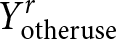 $Y_{{\text{otheruse}}}^r$ is the crop production used for nonfood uses in FABIO. The ${Z_{{\text{link}}}}$ is constructed as
 \begin{equation}\begin{array}{*{20}{c}}
{{Z_{{\text{link}}}} = \left( {\begin{array}{*{20}{c}}
{Z_{{\text{link}}}^1}& \ldots &{Z_{{\text{link}}}^R}
\end{array}} \right)}.
\end{array}\end{equation}
\begin{equation}\begin{array}{*{20}{c}}
{{Z_{{\text{link}}}} = \left( {\begin{array}{*{20}{c}}
{Z_{{\text{link}}}^1}& \ldots &{Z_{{\text{link}}}^R}
\end{array}} \right)}.
\end{array}\end{equation} Here,  ${Z_{{\text{link}}}}$ has 192*123 rows (FABIO) and 164*120 columns (GLORIA). A more detailed description can be found in Bruckner and Kuschnig (Reference Bruckner and Kuschnig2020).
The Leontief inverse  ${B^{ - 1}}$ of the linking table (Bruckner & Kuschnig, Reference Bruckner and Kuschnig2020):
 \begin{equation}\begin{array}{*{20}{c}}
{{B^{ - 1}} = - {A^{ - 1}}B{D^{ - 1}}},
\end{array}\end{equation}
\begin{equation}\begin{array}{*{20}{c}}
{{B^{ - 1}} = - {A^{ - 1}}B{D^{ - 1}}},
\end{array}\end{equation} \begin{equation}\begin{array}{*{20}{c}}
{B = \left( {0 - {A_{{\text{link}}}}} \right)},
\end{array}\end{equation}
\begin{equation}\begin{array}{*{20}{c}}
{B = \left( {0 - {A_{{\text{link}}}}} \right)},
\end{array}\end{equation} \begin{equation}\begin{array}{*{20}{c}}
{A = \left( {I - {A_{{\text{FABIO}}}}} \right)},
\end{array}\end{equation}
\begin{equation}\begin{array}{*{20}{c}}
{A = \left( {I - {A_{{\text{FABIO}}}}} \right)},
\end{array}\end{equation} \begin{equation}\begin{array}{*{20}{c}}
{D = \left( {I - {A_{{\text{GLORIA}}}}} \right)}.
\end{array}\end{equation}
\begin{equation}\begin{array}{*{20}{c}}
{D = \left( {I - {A_{{\text{GLORIA}}}}} \right)}.
\end{array}\end{equation} Here,  $A$ is the direct requirement matrix,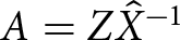 $A = Z{\hat X^{ - 1}}$ and $X$ is the total output for the linking table, FABIO, and GLORIA, respectively. For all the food uses, the crop production involved in international trade ( ${X_{{\text{ctf}}}}$) was calculated by
 \begin{equation}\begin{array}{*{20}{c}}
{{X_{cpt,{\text{ }}food}} = {{\left( {I - {A_{FABIO}}} \right)}^{ - 1}}{Y_{FABIO}}{\text{ }}}
\end{array}\end{equation}
\begin{equation}\begin{array}{*{20}{c}}
{{X_{cpt,{\text{ }}food}} = {{\left( {I - {A_{FABIO}}} \right)}^{ - 1}}{Y_{FABIO}}{\text{ }}}
\end{array}\end{equation} Here, 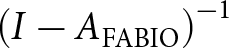 ${\left( {I - {A_{{\text{FABIO}}}}} \right)^{ - 1}}$ is the Leontief inverse of FABIO. ${Y_{{\text{FABIO}}}}$ is the final demand matrix, with one column per country in FABIO, excluding the nonfood uses and ‘balancing’ columns. Crop production involved in trade was derived by isolating the final demand originating from other countries. Similarly, for nonfood uses, the crop production involved in international trade ( ${X_{{\text{ctnf}}}}$) was calculated by
 \begin{equation}\begin{array}{*{20}{c}}
{{X_{cpt,{\text{ }}nonfood}} = {B^{ - 1}}{Y_{GLORIA}}{\text{ }}}
\end{array}\end{equation}
\begin{equation}\begin{array}{*{20}{c}}
{{X_{cpt,{\text{ }}nonfood}} = {B^{ - 1}}{Y_{GLORIA}}{\text{ }}}
\end{array}\end{equation} Here,  ${Y_{{\text{GLORIA}}}}$ is the final demand matrix in GLORIA. We further distinguish the final demand ${Y_{{\text{FABIO}}}}$ into three types of food products (crops as food, crop food products, and animal-sourced human food, Supplementary Materials S.2 for details). In addition to nonfood uses, we have four types of final demand. The sum of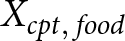 ${X_{cpt,{\text{ }}food}}$ and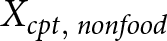 ${X_{cpt,{\text{ }}nonfood}}$ provides the crop production involved in international trade for each country for each of the 61 crop sectors.
2.2. Link the crop production involved in trade to small-scale and large-scale agriculture and virtual water flow calculations
Distinguishing between small-scale and large-scale agriculture in international trade and virtual water flow is challenging due to limited subnational trade data. Although market access to small-scale and large-scale agriculture could be retrieved from household surveys, it is only available for a few countries (FAO, 2021). Small-scale farmers in particular may experience limited access to formal markets, especially international markets (Giller et al., Reference Giller, Delaune, Silva, Descheemaeker, van de Ven, Schut, van Ittersum, Hammond, Hochman, Taulya, Chikowo, Narayanan, Kishore, Bresciani, Teixeira, Andersson and van Ittersum2021). We allocate the total production involved in international trade per crop sector per country to small-scale and large-scale agriculture using two commonly used assumptions in the literature: the production-based assumption (Sun et al., Reference Sun, Tukker and Behrens2019) and the farming system-based assumption (Hoang et al., Reference Hoang, Taherzadeh, Ohashi, Yonekura, Nishijima, Yamabe, Kanemoto, Matsuda, Moran and Kanemoto2023). The production-based assumption allocates crop production (domestic or export) to small-scale and large-scale agriculture solely on their production, regardless of any other factors. The farming system-based assumption suggests that irrigated and high-input farming systems have significantly better access to export markets than the low-input farming system. This assumption allocates the export first to irrigated and high-input farming systems, and then to the low-input farming system. Since the low-input farming system could still be export-oriented, this assumption may overestimate the contribution of irrigated and high-input farming systems to international trade. Using both assumptions provides upper and lower bounds for estimating the contribution of different farming systems to virtual water flows.
Under the production-based assumption, the crop production involved in trade is allocated to small-scale and large-scale agriculture proportionally based on their crop production:
 \begin{equation}\begin{array}{*{20}{c}}
{{cp}{t}_{s,ih}} = {c}{{p}_{s,ih}}*\frac{{cp}{{t}_{{total}}}}{{{c}{{p}_{total}}}},
\end{array}\end{equation}
\begin{equation}\begin{array}{*{20}{c}}
{{cp}{t}_{s,ih}} = {c}{{p}_{s,ih}}*\frac{{cp}{{t}_{{total}}}}{{{c}{{p}_{total}}}},
\end{array}\end{equation} \begin{equation}\begin{array}{*{20}{c}}
cpt_{s,low}=cp_{s,low}*\frac{{cp}{{t}_{{total}}}}{{{c}{{p}_{total}}}},
\end{array}\end{equation}
\begin{equation}\begin{array}{*{20}{c}}
cpt_{s,low}=cp_{s,low}*\frac{{cp}{{t}_{{total}}}}{{{c}{{p}_{total}}}},
\end{array}\end{equation} \begin{equation}\begin{array}{*{20}{c}}
{{cp}{{t}_{l,ih}} = {c}{{p}_{l,ih}}*\frac{{{cp}{{t}_{{total}}}}}{{{c}{{p}_{{total}}}}},}
\end{array}\end{equation}
\begin{equation}\begin{array}{*{20}{c}}
{{cp}{{t}_{l,ih}} = {c}{{p}_{l,ih}}*\frac{{{cp}{{t}_{{total}}}}}{{{c}{{p}_{{total}}}}},}
\end{array}\end{equation} \begin{equation}\begin{array}{*{20}{c}}
{{cp}{{t}_{l,low}} = {c}{{p}_{l,lows}}*\frac{{{cp}{{t}_{{total}}}}}{{{c}{{p}_{{total}}}}}.}
\end{array}\end{equation}
\begin{equation}\begin{array}{*{20}{c}}
{{cp}{{t}_{l,low}} = {c}{{p}_{l,lows}}*\frac{{{cp}{{t}_{{total}}}}}{{{c}{{p}_{{total}}}}}.}
\end{array}\end{equation} where  ${\text{cp}}$ and ${\text{cpt}}$ are crop production and the crop production involved in trade, respectively. The subscript $s$ indicates small-scale agriculture; $l$ indicates large-scale agriculture; $ih$ indicates irrigated and high-input farming system; ${\text{low}}$ indicates the low-input farming system. Thus, ${\text{cp}}{{\text{t}}_{s,ih}}$ indicates the crop production involved in trade from small-scale agriculture and from irrigated and high-input farming systems.
Under the farming system-based assumption, we first allocate the crop production involved in trade to the irrigated and high-input rain-fed farming systems and then distribute it proportionately between small-scale and large-scale agriculture, based on their respective production in irrigated and high-input rain-fed farming systems. If the volume of crop production involved in trade exceeds the combined production from irrigated and high-input farming systems, the surplus is allocated to small-scale and large-scale agriculture according to their respective production in the low-input farming system. When  ${\text{cp}}{{\text{t}}_{{\text{total}}}} \lt {\text{c}}{{\text{p}}_{s,ih}} + {\text{c}}{{\text{p}}_{l,ih}},$
 \begin{equation}\begin{array}{*{20}{c}}
{{cp}{{t}_{s,ih}} = {c}{{p}_{s,ih}}*\frac{{{cp}{{t}_{{total}}}}}{{{c}{{p}_{s,ih}} + {c}{{p}_{l,ih}}}}},
\end{array}\end{equation}
\begin{equation}\begin{array}{*{20}{c}}
{{cp}{{t}_{s,ih}} = {c}{{p}_{s,ih}}*\frac{{{cp}{{t}_{{total}}}}}{{{c}{{p}_{s,ih}} + {c}{{p}_{l,ih}}}}},
\end{array}\end{equation} \begin{equation}\begin{array}{*{20}{c}}
{{cp}{{t}_{s,{low}}} = 0},
\end{array}\end{equation}
\begin{equation}\begin{array}{*{20}{c}}
{{cp}{{t}_{s,{low}}} = 0},
\end{array}\end{equation} \begin{equation}\begin{array}{*{20}{c}}
{{cp}{{t}_{l,ih}} = {c}{{p}_{l,ih}}*\frac{{{cp}{{t}_{{total}}}}}{{{c}{{p}_{s,ih}} + {c}{{p}_{l,ih}}}}},
\end{array}\end{equation}
\begin{equation}\begin{array}{*{20}{c}}
{{cp}{{t}_{l,ih}} = {c}{{p}_{l,ih}}*\frac{{{cp}{{t}_{{total}}}}}{{{c}{{p}_{s,ih}} + {c}{{p}_{l,ih}}}}},
\end{array}\end{equation} \begin{equation}\begin{array}{*{20}{c}}
{{cp}{{t}_{l,{low}}} = 0}.
\end{array}\end{equation}
\begin{equation}\begin{array}{*{20}{c}}
{{cp}{{t}_{l,{low}}} = 0}.
\end{array}\end{equation}Otherwise:
 \begin{equation}\begin{array}{*{20}{c}}
{{cp}{{t}_{s,ih}} = {c}{{p}_{s,ih}}},
\end{array}\end{equation}
\begin{equation}\begin{array}{*{20}{c}}
{{cp}{{t}_{s,ih}} = {c}{{p}_{s,ih}}},
\end{array}\end{equation} \begin{equation}\begin{array}{*{20}{c}}
{{cp}{{t}_{s,{low}}} = {c}{{p}_{s,{low}}}*\frac{{{cp}{{t}_{{total}}} - {c}{{p}_{s,ih}} - {c}{{p}_{l,ih}}}}{{{c}{{p}_{{total}}} - {c}{{p}_{s,ih}} - {c}{{p}_{l,ih}}}} = {c}{{p}_{s,low}}*\frac{{{cp}{{t}_{{total}}} - {c}{{p}_{s,ih}} - {c}{{p}_{l,ih}}}}{{{c}{{p}_{s,{low}}} + {c}{{p}_{l,{low}}}}},}
\end{array}\end{equation}
\begin{equation}\begin{array}{*{20}{c}}
{{cp}{{t}_{s,{low}}} = {c}{{p}_{s,{low}}}*\frac{{{cp}{{t}_{{total}}} - {c}{{p}_{s,ih}} - {c}{{p}_{l,ih}}}}{{{c}{{p}_{{total}}} - {c}{{p}_{s,ih}} - {c}{{p}_{l,ih}}}} = {c}{{p}_{s,low}}*\frac{{{cp}{{t}_{{total}}} - {c}{{p}_{s,ih}} - {c}{{p}_{l,ih}}}}{{{c}{{p}_{s,{low}}} + {c}{{p}_{l,{low}}}}},}
\end{array}\end{equation} \begin{equation}\begin{array}{*{20}{c}}
{{cp}{{t}_{l,ih}} = {c}{{p}_{l,ih}}},
\end{array}\end{equation}
\begin{equation}\begin{array}{*{20}{c}}
{{cp}{{t}_{l,ih}} = {c}{{p}_{l,ih}}},
\end{array}\end{equation} \begin{equation}\begin{array}{*{20}{c}}
{{cp}{{t}_{l,{low}}} = c{p_{l,{lows}}}*\frac{{{cp}{{t}_{{total}}} - {c}{{p}_{s,ih}} - {c}{{p}_{l,ih}}}}{{{c}{{p}_{{total}}} - {c}{{p}_{s,ih}} - {c}{{p}_{l,ih}}}} = c{p_{l,{lows}}}*\frac{{{cp}{{t}_{{total}}} - {c}{{p}_{s,ih}} - {c}{{p}_{l,ih}}}}{{{c}{{p}_{s,{low}}} + {c}{{p}_{l,{low}}}}}}.
\end{array}\end{equation}
\begin{equation}\begin{array}{*{20}{c}}
{{cp}{{t}_{l,{low}}} = c{p_{l,{lows}}}*\frac{{{cp}{{t}_{{total}}} - {c}{{p}_{s,ih}} - {c}{{p}_{l,ih}}}}{{{c}{{p}_{{total}}} - {c}{{p}_{s,ih}} - {c}{{p}_{l,ih}}}} = c{p_{l,{lows}}}*\frac{{{cp}{{t}_{{total}}} - {c}{{p}_{s,ih}} - {c}{{p}_{l,ih}}}}{{{c}{{p}_{s,{low}}} + {c}{{p}_{l,{low}}}}}}.
\end{array}\end{equation}The virtual water flow was calculated using unit blue and green water consumption for small-scale and large-scale agriculture, per farming system, and crop. Crop production and water consumption data for small-scale and large-scale agriculture were retrieved from Su et al. (Reference Su, Foster, Hogeboom, Luna-Gonzalez, Mialyk, Willaarts and Krol2025b). This dataset covers 171 crops from 55 countries between 2008 and 2012 (Supplementary Materials S.1), which were aggregated into FABIO 61 crop sectors (Supplementary Materials S.3). While other datasets provide a more extensive global coverage than this dataset in terms of crop production, e.g., Herrero et al. (Reference Herrero, Thornton, Power, Bogard, Remans, Fritz, Havlík, Nelson, See, Waha, Watson, West, Samberg, van de Steeg, Stephenson, van Wijk and Havlík2017) and Mehrabi et al. (Reference Mehrabi, McDowell, Ricciardi, Levers, Martinez, Mehrabi, Jarvis, Ramankutty and Jarvis2020), they were developed for the year 2000 cropland and, more importantly, do not provide corresponding water consumption and farming system data. The farming system-based assumption requires distinguishing between low-input and high-input farming systems in the crop map dataset. SPAM2010 is the latest version containing this information and is covered by the dataset of Su et al. (Reference Su, Foster, Hogeboom, Luna-Gonzalez, Mialyk, Willaarts and Krol2025b). The dataset of Su et al. (Reference Su, Foster, Hogeboom, Luna-Gonzalez, Mialyk, Willaarts and Krol2025b) provides the estimated crop production and water consumption per grid cell, farming system, and crop for both small-scale and large-scale agriculture, based on underlying regional agricultural census data. In this dataset, small-scale agriculture was identified by the combination of three definitions: a 2-ha threshold (below 2 ha farm size), a subsistence farming system, and the SDG 2.3.2 definition (the smallest farms that contribute 40% of national cropland and 40% of agriculture revenue). The remaining part is classified as large-scale agriculture, which includes both medium- and large-scale agriculture (Su et al., Reference Su, Foster, Hogeboom, Luna-Gonzalez, Mialyk, Willaarts and Krol2025b). Virtual water flow was calculated by multiplying unit water consumption by the crop production involved in trade for small-scale and large-scale agriculture, respectively.
3. Results
3.1. The contribution of small-scale agriculture to crop production involved in trade
Overall, small-scale agriculture contributes only about 17% of the total crop production involved in trade (in tonnes), among the 55 countries analyzed. However, its contribution is significantly higher for several cash crops (Table 1). For example, based on the farming system assumption, small-scale agriculture accounts for 75% of fiber crop production involved in global trade. In addition, small-scale agriculture also contributes significantly to coffee, tea, and cocoa (49%); tobacco and rubber (43%); roots and tubers (36%); cereals (26%); vegetables, fruit, nuts, pulses, and spices (25%); and oil crops (24%). Many of these crops are labor-intensive and less well-suited to mechanized agriculture. In contrast, small-scale agriculture contributes substantially less to the production of fodder crops and sugar crops involved in trade, which are dominated by large-scale agriculture.
The crop production involved in trade by small-scale and large-scale agriculture from 55 countries, based on the farming system assumption
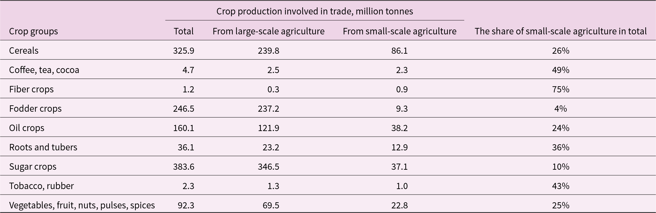
Table 1 Long description
The table reports traded crop production volumes for several crop groups across 55 countries, split into amounts from large-scale and small-scale agriculture, plus the small-scale share of each group’s total. Sugar crops have the highest traded production at 383.6 million tonnes, mostly from large-scale farms at 346.5 million tonnes, with small-scale contributing 37.1 million tonnes for a 10% share. Cereals total 325.9 million tonnes, with 239.8 from large-scale and 86.1 from small-scale, giving small-scale a 26% share. Fodder crops are also very large at 246.5 million tonnes but are overwhelmingly large-scale at 237.2 million tonnes, leaving small-scale at 9.3 million tonnes and a 4% share. The highest small-scale shares occur in fibre crops at 75% and coffee, tea, cocoa at 49%, while tobacco and rubber are 43% and roots and tubers are 36%. Vegetables, fruit, nuts, pulses, and spices total 92.3 million tonnes with a 25% small-scale share, and oil crops total 160.1 million tonnes with a 24% small-scale share. These figures reflect production involved in trade under a specific farming-system assumption and may not represent all production or all countries.
The production-based assumption provides similar results. By comparing the two assumptions, there are minor differences in the allocation of crop production involved in trade between small-scale and large-scale agriculture at the national level (Supplementary Materials S.4). Specifically, for the crop production of large-scale agriculture involved in trade, the two assumptions produce nearly identical national-level estimates. In contrast, the differences are more pronounced for small-scale agriculture, particularly in developing countries where the export volume is low. The farming system-based assumption generally allocates slightly less crop production involved in trade to small-scale agriculture (typically <4% for each crop group).
3.2. The contribution of small-scale agriculture to virtual water flows
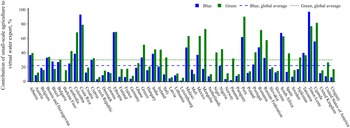
Under both assumptions, small-scale agriculture accounts for approximately 22% of blue and 30% of green virtual water flows, which is higher than its contribution to the crop production involved in trade. The relatively lower blue water contribution reflects the lower blue water consumption of small-scale agriculture on the production side. The contribution varies substantially among countries (Figure 1). In many countries, small-scale agriculture accounts for a large share of virtual water exports. It accounts for more than 90% of blue virtual water exports in Costa Rica and more than half in Peru, South Africa, Uganda, Ethiopia, and Timor-Leste. In terms of green water, small-scale agriculture contributes over 90% in Peru and over half in Costa Rica, South Africa, Uganda, Ethiopia, Timor-Leste, Mongolia, Romania, Colombia, Mexico, Malawi, Russia, and Greece, across low-income, middle-income, and high-income countries. For Greece, about 40% of small-scale agriculture’s contribution to green virtual water export comes from olive production (Su et al., Reference Su, Bruckner, Taherzadeh, Sun, Hogeboom, Hongyi and Krol2025a).
The contribution of small-scale agriculture to blue and green virtual water exports at the country level according to the farming system-based assumption. The production-based assumption provides similar spatial patterns.
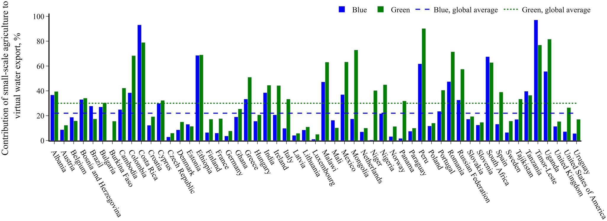
Figure 1 Long description
The bar graph compares blue and green virtual water exports from small-scale agriculture across multiple countries. The x-axis lists countries including Costa Rica, Peru, South Africa, Uganda, Ethiopia, Timor-Leste, Mongolia, Romania, Colombia, Mexico, Malawi, Russia and Greece. The y-axis is labeled 'Contribution of small-scale agriculture to virtual water export (%)' and ranges from 0 to 100 percent. Each country has two bars: one for blue water and one for green water. The legend identifies blue and green bars, along with dashed lines representing the blue and green global averages. Countries like Costa Rica and Peru show high contributions, with values exceeding 90 percent for blue water exports. Many countries, such as Greece, have significant contributions to green water exports, often above 50 percent. The graph highlights that small-scale agriculture plays a substantial role in virtual water exports, with several countries surpassing global averages.
The larger contribution of small-scale agriculture to virtual water flows can be explained by the type of crops it supplies to international trade. For example, fodder crops generally consume less blue and green water per unit of crop production. Large-scale agriculture is more involved in fodder crops; thus, its relative contribution to virtual water flows is lower. At the same time, many cash crops are water-intensive, increasing the relative contribution of small-scale agriculture to virtual water flows.
Differences between blue and green virtual water contributions are influenced by several factors in our estimates, e.g., crop type and farming system. For example, if small-scale agriculture does not consume blue water, e.g., no irrigation, then it may contribute significantly to green virtual water export compared to blue. In addition, small-scale agriculture generally consumes more green water per unit of crop production because of lower inputs to agriculture. This pattern is evident in many African countries. At the same time, though many cash crops do not consume much blue water, they consume a substantial amount of green water per unit of production. This also results in the difference between blue and green virtual water flows.
The contribution of small-scale agriculture to virtual water flows does not necessarily correlate with its contribution to domestic water consumption. In Nigeria, small-scale agriculture consumes about 52% of crop-related domestic blue water; however, it contributes only 22% of blue virtual water exports. At the same time, small-scale agriculture contributes 23% of (crop-related) domestic blue water consumption in Russia, but 33% of blue virtual water flows.
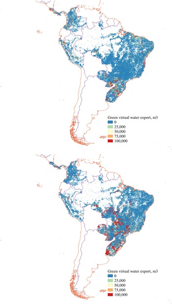
Our results indicate that the spatial pattern of virtual water export differs significantly between small-scale and large-scale agriculture. For example, in Brazil, the green virtual water exports from small-scale agriculture are estimated to largely originate in the Northeast and Southwest Brazil; at the same time, for large-scale agriculture, the green virtual water exports are estimated to originate from middle Brazil (Figure 2). This highlights the importance of distinguishing between small-scale and large-scale agriculture in virtual water flow analysis. Agricultural policies informed by virtual water flow analysis may not only have different impacts on small-scale and large-scale agriculture but also uneven spatial impacts, as shown in the case of Brazil.
The green virtual water exports from small-scale (a) and large-scale agriculture (b) according to the farming system-based assumption in Latin America.
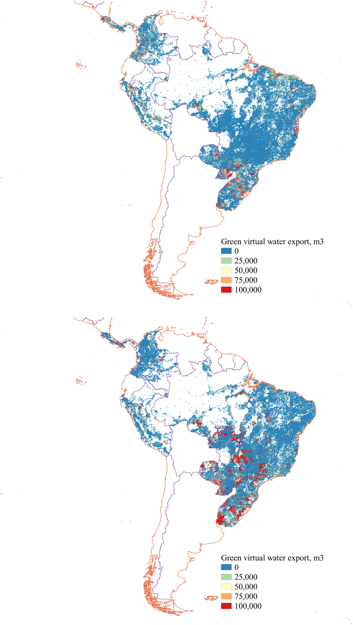
Figure 2 Long description
Two vertically stacked thematic maps of South America. North is at the top. Each map includes internal country boundaries and a legend titled “Green virtual water export, m3”. The legend shows five classes with a light-to-dark progression: 0, 25,000, 50,000, 75,000, 100,000. A) The upper map uses the five legend classes to show the mapped variable across South America. Large areas are in the 0 class, especially along much of the western side and the far south. The strongest concentration of non-zero classes forms a broad zone across the eastern half of the continent, with many areas in the 25,000 and 50,000 classes and scattered patches in the 75,000 and 100,000 classes. The highest class (100,000) appears as small, isolated patches within the eastern zone. B) The lower map uses the same legend and geographic extent. The 0 class again covers much of the western side and the far south. Compared with A, there are more visible patches in the higher classes (75,000 and 100,000) within the eastern half of the continent, including a denser cluster of the highest class in the east-central to southeastern portion. The 25,000 and 50,000 classes remain widespread across the eastern half, surrounding the higher-class patches.
The farming system-based assumption often results in higher blue virtual water exports and lower green virtual water exports (Supplementary Materials S.4). This is the consequence of the fact that irrigated and high-input farming systems consume more blue water but less green water due to the high water use efficiency. Since the farming system-based assumption allocates slightly less export to small-scale agriculture, the contribution of small-scale agriculture to blue and green virtual water flows is also slightly lower than that under the production-based assumption.
3.3. Sectoral drivers of virtual water trade
At the global level, the largest final demand driving small-scale agriculture’s blue and green virtual water export is crops used directly as food (Figure 3, Supplementary Materials S.5), as cereals are generally more traded than other crops. The second largest final demand associated with small-scale agriculture’s virtual water export is nonfood uses for blue and animal-sourced human food for green. The nonfood uses primarily refer to fiber crops for textiles, crops for biofuels, and crops as feed for livestock, which ultimately produce nonfood products, for example, leather. These two final demands drive about 70% of small-scale agriculture’s contribution to blue/green virtual water flows. The two dominant final demand categories driving small-scale agriculture’s virtual water exports may differ across countries. For example, final demand for crop food products is the largest driver of small-scale agriculture’s blue virtual water exports in Costa Rica and Italy; in Mali, almost all of small-scale agriculture’s blue virtual water exports are driven by nonfood uses.
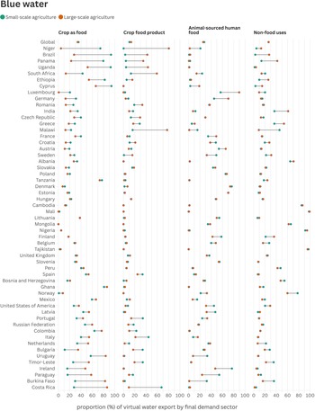
Share of the four final demand sectors associated with the blue virtual water export of small-scale and large-scale agriculture according to the farming system-based assumption, sorted by the difference between small-scale and large-scale agriculture in crops as food share. The production-based assumption provides similar patterns. The four final demand values sum to 100% for small-scale and large-scale agriculture, respectively. The corresponding figure in green water can be found in Supplementary Materials S.5.
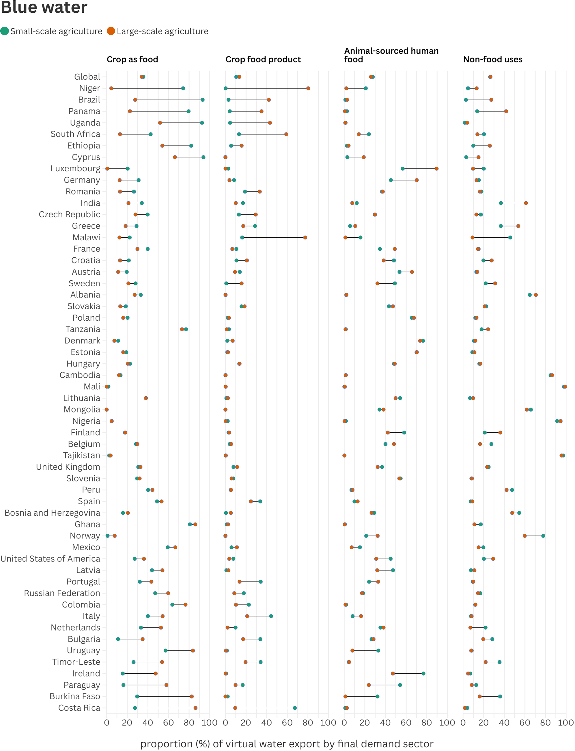
Figure 3 Long description
The image shows four dot plots comparing blue water virtual water export proportions by final demand sector across countries. The sectors are 'Crop as food,' 'Crop food product,' 'Animal-sourced human food,' and 'Non-food uses.' Each plot compares small-scale agriculture (green dots) and large-scale agriculture (orange dots). The x-axis is labeled 'proportion (percent) of virtual water export by final demand sector,' ranging from 0 to 100 percent. The y-axis lists countries, including Global, Niger, Brazil, Panama, Uganda, South Africa, Ethiopia, Cyprus, Luxembourg, Germany, Romania, India, Czech Republic, Greece, Malawi, France, Croatia, Austria, Sweden, Albania, Slovakia, Poland, Tanzania, Denmark, Estonia, Hungary, Cambodia, Mali, Lithuania, Mongolia, Nigeria, Angola, Finland, Belgium, Tajikistan, United Kingdom, Slovenia, Peru, Spain, Bosnia and Herzegovina, Ghana, Norway, Mexico, United States of America, Latvia, Portugal, Russian Federation, Colombia, Italy, Netherlands, Thailand, Bulgaria, Uruguay, Timor-Leste, Ireland, Paraguay, Burkina Faso, Costa Rica. Notable observations include Costa Rica showing high proportions for small-scale agriculture in 'Crop as food,' while Niger shows a large gap between small and large-scale agriculture in 'Non-food uses.' Most countries cluster below 50 percent in 'Animal-sourced human food.' The plots reveal differences in virtual water export proportions between small and large-scale agriculture, with varying trends across sectors and countries.
The final demand sectors driving virtual water exports differ between small-scale and large-scale agriculture (Figure 3, Supplementary Materials S.5). Demand for crops as food is generally a stronger driver for blue and green virtual water export for small-scale agriculture than for large-scale agriculture. Where this is not the case, demand for crop food products shows a stronger driver in small-scale agriculture than in large-scale agriculture. Although demand for crops as food and crop food products still accounts for a significant share, demand for animal-sourced human food and nonfood uses represents a higher proportion in large-scale agriculture than in small-scale agriculture, both at the global level and across the majority of the 55 countries. Nonfood uses and animal-sourced human foods are generally associated with higher-value products than crops used directly as food. This suggests that small-scale agriculture may benefit less from high-value products, and that its contribution might be driven primarily by demand for labor-intensive crops.
4. Discussion
4.1. Policy implications
Understanding the involvement of small-scale and large-scale agriculture in trade helps design more context-specific policies. For example, our results show that small-scale agriculture’s contribution is prominent in many cash crop-related virtual water flows, where large corporations are more prominent as well (Baronchelli et al., Reference Baronchelli, Vallino, Dalmazzone, Ridolfi and Laio2024). This makes policy interventions involving both farmers and corporations more challenging, given the unequal power dynamics. This inequality is further compounded by the type of water resource controlled. Smallholders are more likely to rely on rain-fed systems and green water. Because green water is not easily managed through traditional economic instruments like water pricing, smallholders face unique vulnerabilities that corporate-centric policies often overlook. Interventions must therefore account for these distinct water-use profiles to avoid placing undue burdens on the small-scale producers.
This economic marginalization is mirrored in market pricing. Water scarcity, which disproportionately affects small-scale agriculture (Ricciardi et al., Reference Ricciardi, Wane, Sidhu, Godde, Solomon, McCullough, Mehrabi, Porciello, Jain, Randall and Mehrabi2020; Su et al., Reference Su, Willaarts, Luna-Gonzalez, Krol and Hogeboom2022), is less embedded in the crop price for cash crops (Falsetti et al., Reference Falsetti, Vallino, Ridolfi and Laio2020). This indicates that the value of water is substantially underestimated for these crops. Unlike large-scale farms, small-scale farms are generally not specialized (Fan & Rue, Reference Fan and Rue2020; Frelat et al., Reference Frelat, Lopez-Ridaura, Giller, Herrero, Douxchamps, Djurfeldt, Paul, Henderson, Kassie, Paul, Rigolot, Ritzema, Rodriguez, van Asten and van Wijk2016; Ricciardi et al., Reference Ricciardi, Mehrabi, Wittman, James and Ramankutty2021). They often rely on a more diverse mix of on-farm (e.g., multiple crops or crop-livestock systems rather than a single crop) and off-farm income sources (Frelat et al., Reference Frelat, Lopez-Ridaura, Giller, Herrero, Douxchamps, Djurfeldt, Paul, Henderson, Kassie, Paul, Rigolot, Ritzema, Rodriguez, van Asten and van Wijk2016). This implies that they may have fewer incentives to improve water use efficiency compared to large-scale farmers, which means that policy interventions may not only focus on crop production, but also on other activities that small-scale farmers are involved in.
Our results also highlight the limitations of the current virtual water flow assessment, which overlooks interactions between small-scale and large-scale agriculture. For example, countries may want to reduce their external water consumption by improving the water use efficiency of imported products (Hoekstra & Mekonnen, Reference Hoekstra and Mekonnen2016). Such a supply-chain-oriented policy could, in light of our findings, encourage greater investment in already-efficient large-scale agriculture. These efficient large-scale farming systems may expand based on the assumption that they can save global water use via transboundary food trade, but this expansion, driven by foreign investment, may compete with the water availability of small-scale farmers (Chiarelli et al., Reference Chiarelli, D'Odorico, Muller, Mueller, Davis, Dell'Angelo and Rulli2022; Dalin et al., Reference Dalin, Konar, Hanasaki, Rinaldo and Rodriguez-Iturbe2012; Hoekstra, Reference Hoekstra2020) and lead to greater consolidation of food production. Distinguishing the farms involved in virtual water flows can help guide policies that balance poverty reduction, food security, and water sustainability.
4.2. Uncertainties and limitations
Many factors influence the relative contribution of small-scale and large-scale agriculture to international trade and virtual water flows. The difference in virtual water flows in our study mainly comes from crop structure and farming systems in small-scale and large-scale agriculture, and the crop water footprint of different farming systems. If small-scale and large-scale farms produce the same crop with the same farming system, our method cannot distinguish between them without additional information, e.g., export market access.
Based on the assumption that irrigated and high-input farming systems are more export-oriented than low-input and subsistence farming systems, we estimated that small-scale agriculture makes a significant contribution to virtual water flows. This represents a substantial share of blue and green water consumption, and our estimates do not conflict with current household surveys, showing the majority of small-scale agricultural crop production was sold (FAO, 2023a; Malek & Verburg, Reference Malek and Verburg2020; Rapsomanikis, Reference Rapsomanikis2015).
The countries studied cover around half of global cropland (Su et al., Reference Su, Willaarts, Luna-Gonzalez, Krol and Hogeboom2022). The virtual water flows from crops in 55 countries account for roughly 30% of global blue virtual water and 50% of global green virtual water (Graham et al., Reference Graham, Hejazi, Kim, Davies, Edmonds and Miralles-Wilhelm2020; Hoekstra & Mekonnen, Reference Hoekstra and Mekonnen2012; Mekonnen & Hoekstra Reference Mekonnen and Hoekstra2020). Our analysis is based on harvested areas, crop production, and water consumption in small-scale and large-scale agriculture instead of the number of farms and farmers. We do not include livestock or industrial sectors, which account for a considerable amount of virtual water flows but are outside the scope of this study. We included the virtual water flows of crops as feed in livestock exports.
The reliability of virtual water flow estimates depends on the reliability of the input–output table (FABIO) and the crop water footprint. FABIO was established using FAOSTAT data (FAO, 2023b) for food products (Bruckner et al., Reference Bruckner, Wood, Moran, Kuschnig, Wieland, Maus and Borner2019). The water footprints of crops were retrieved from and validated by Su et al. (Reference Su, Foster, Hogeboom, Luna-Gonzalez, Mialyk, Willaarts and Krol2025b). Our estimates of blue virtual water flows from soybean and sugar crops in Brazil, based on the two assumptions, could cover the estimates from the previous study (59 million and 850 million m3) that incorporated subnational international trade information. Compared to the studies incorporating local information and using more sophisticated models to estimate the trade direction, e.g., Flach et al. (Reference Flach, Ran, Godar, Karlberg and Suavet2016) and Pandit et al. (Reference Pandit, Karakoc and Konar2023), we do not differentiate export destinations from subnational regions; our method requires less detailed information but covers more countries.
While our dual-assumption approach (production-based and farming system-based) provides a robust range for current estimates, precisely distinguishing farm-level contributions in complex global supply chains remains a methodological frontier. Future research could overcome these challenges by integrating emerging technologies such as satellite-based crop monitoring and blockchain-verified supply chain data. These tools could eventually allow for the direct tracking of commodities from specific farm sizes to final consumers, reducing the need for proxy-based allocations.
5. Conclusion
Small-scale agriculture plays an important role in international trade and exports virtual water through the production of many crops, except fodder crops and sugar crops. Across all crops, small-scale agriculture accounts for 22% of blue and 30% of green virtual water flows, which is higher than its share of crop production involved in trade. Although the estimates at the country and sector levels involve certain uncertainties, they show consistent patterns at the global level, as demonstrated by the comparison of our two assumptions. Nevertheless, our findings provide valuable insights into how virtual water flow assessment can help to identify the role of small-scale agriculture in global food and water security. The findings also underscore the importance of considering the agricultural heterogeneity in virtual water flow assessments to improve the targeting of interventions.
Supplementary material
The supplementary material for this article can be found at https://doi.org/10.1017/sus.2026.10066.
Acknowledgements
We thank the reviewers and editor for the insightful comments that helped us improve the quality of the article.
Author contributions
H.S., M.B., O.T., Z.S., R.J.H., and M.S.K. designed the research. H.S. and M.B. conducted the research. H.S., O.T., and H.C. analyzed the data. H.S., M.B., O.T., Z.S., R.J.H., H.C., and M.S.K. wrote the paper.
Funding statement
This research was supported by the H2020 European Research Council (Advanced Grant 2018 [grant no. 834716]). R.H. was supported by the Dutch Research Council (NWO) Talentprogramma 2022 (Vl.Veni.221S.080). Z.S. was supported by the National Natural Science Foundation of China (grant no. 52200222), the Key Project of Philosophy and Social Sciences of China’s Ministry of Education (grant no. 22JZD019), and the 2115 Talent Development Program of China Agricultural University. O.T. and H.C. were supported by the H2020 Research and Innovation Programme (GreenGrocer project, grant no. 101182025).
Competing interests
The authors have no competing interests to declare.
Code and data availability
The country- and crop-level estimates of crop production involved in trade and virtual water flows estimated by this study are freely available via a Creative Commons Attribution 4.0 International license at the DOI: https://doi.org/10.4121/4d32300f-28cf-45f8-8e9d-77759bf6e9ce (Su et al., Reference Su, Bruckner, Taherzadeh, Sun, Hogeboom, Hongyi and Krol2025a). All code, input data, and output data required to reproduce the results in this study will be archived for at least 10 years after publication within the University of Twente, Multidisciplinary Water Management (MWM) group. The MWM group will make the code and data available upon request.



 Open access

