





1. Introduction
The white dwarf star ZTF J203349.8+322901.1 is highly unusual, in that it appears to have hemispheres with surfaces, respectively, dominated by hydrogen and helium. As the star rotates ( $P=14.97$
min), its spectrum changes from one dominated by H lines to one dominated by He absorption. Ciazzo et al. (2023) propose that the star is at an evolutionary stage where it cools and its atmosphere transitions from being H-rich to being He-dominated, the He brought to surface by convection. In the case of ZTF J203349.8+322901.1 a weak, undetected magnetic field may be be suppressing convection in the H-rich hemisphere. Ciazzo et al. (2023) propose three other candidates for this type of peculiar abundance configuration, one of which is the well-known magnetic white dwarf Feige 7.
$P=14.97$
min), its spectrum changes from one dominated by H lines to one dominated by He absorption. Ciazzo et al. (2023) propose that the star is at an evolutionary stage where it cools and its atmosphere transitions from being H-rich to being He-dominated, the He brought to surface by convection. In the case of ZTF J203349.8+322901.1 a weak, undetected magnetic field may be be suppressing convection in the H-rich hemisphere. Ciazzo et al. (2023) propose three other candidates for this type of peculiar abundance configuration, one of which is the well-known magnetic white dwarf Feige 7.
Feige 7 (BV Cet, PHL 814, PB 8504, WD 0041-102) was identified as a magnetic He-rich white dwarf by Liebert et al. (Reference Liebert, Angel, Stockman, Spinrad and Beaver1977), who also reviewed the earlier literature on the star. The authors estimated a mean magnetic field strength of close to 18 MG, with little variation with rotation phase. Circular polarisation radiation was found to vary cyclically with a period of 2.2 h, ascribed to rotation. Photometry obtained by Achilleos et al. (Reference Achilleos, Wickramasinghe, Liebert, Saffer and Grauer1992) showed the same periodicity, implying a non-uniform surface brightness.
Liebert et al. (Reference Liebert, Angel, Stockman, Spinrad and Beaver1977) note that ‘the spectrum changes associated with rotation are rather slight’ and conclude that there is no compelling evidence for variations in the H and He surface abundances in the star. Achilleos et al. (Reference Achilleos, Wickramasinghe, Liebert, Saffer and Grauer1992), on the other hand, find that the He/H abundance ratio needs to vary by orders of magnitude in order to account for the changes of spectral lines over the 2.2 h cycles; 10–100 $\unicode{x003C}$
[He/H]
$\unicode{x003C}$
[He/H] $\unicode{x003C}$
100–500 are quoted. The authors were also able to model the amplitude of the brightness changes they observed in the V filter as being due to inhomogeneities in the surface He/H ratio. The required magnetic field strength in their models is about double that of the Liebert et al. (Reference Liebert, Angel, Stockman, Spinrad and Beaver1977) estimate.
$\unicode{x003C}$
100–500 are quoted. The authors were also able to model the amplitude of the brightness changes they observed in the V filter as being due to inhomogeneities in the surface He/H ratio. The required magnetic field strength in their models is about double that of the Liebert et al. (Reference Liebert, Angel, Stockman, Spinrad and Beaver1977) estimate.
It has been shown (Tremblay et al. 2015; Gentile Fusillo et al. 2018) that even relatively weak magnetic fields (well below 1 MG) strongly inhibit convection in white dwarf stars. The mechanism giving rise to the chemical inhomogeneity is therefore not obvious. A possible resolution of the problem has been provided by Moss et al. (2023): convection across magnetic field lines is suppressed, but may take place parallel to the field. This could then give rise to chemical ‘patchiness’ on the stellar surface.
The principal aim of the present paper is to test whether abundance inhomogeneities could explain the photometric amplitude changes seen in several different filters.
2. Physical properties of Feige 7
Hardy, Dufour, & Jordan (Reference Hardy, Dufour and Jordan2023b) compared ‘Sloan Digital Sky Survey’ ugriz photometry to synthetic photometry, to derive $T_\mathrm{eff}=20\,848 (1\,077)$
K,
$T_\mathrm{eff}=20\,848 (1\,077)$
K, $\log\;g=8.86 (0.18)$
. The surface composition was assumed to be pure Helium. The derived mass of Feige 7 is 1.13(0.18) M
$\log\;g=8.86 (0.18)$
. The surface composition was assumed to be pure Helium. The derived mass of Feige 7 is 1.13(0.18) M $_\odot$
.
$_\odot$
.
A noteworthy feature of the Hardy et al. (Reference Hardy, Dufour and Jordan2023b) synthetic photometry is that it takes into account the spectral line shifts due to the strong magnetic field; this Zeeman effect causes strong absorption features to be shifted into or out of photometric bandpasses. A more detailed discussion can be found in Hardy, Dufour, & Jordan (Reference Hardy, Dufour and Jordan2023a). As an alternative, we use synthetic photometry uncorrected for magnetic effects, but over a much wider wavelength region ( $1\,516 \le \lambda_\mathrm{eff} \le 21\,500$
Å) and including 22 different filters for which observations are available.
$1\,516 \le \lambda_\mathrm{eff} \le 21\,500$
Å) and including 22 different filters for which observations are available.
Collected standardised photometry of Fiege 7 was obtained from the VizieR serviceFootnote a of the Strasbourg astronomical Data Center. Original sources of the data are APASS (‘AAVSO Photometric All-Sky Survey’, Henden et al. Reference Henden, Levine and Terrell2015), Gaia (Gaia collaboration 2021), Pan-STARRS (‘The Panoramic Survey Telescope and Rapid Response System’, Chambers et al. 2016), GALEX (‘Galaxy Evolution Explorer’, Bianchi et al. 2017), 2MASS (‘Two Micron All-Sky Survey’, Skrutskie et al. 2006) and WISE (‘Wide-field Infrared Survey Explorer’, Wright et al. Reference Wright, Eisenhardt and Mainzer2010). The efforts of these surveys are gratefully acknowledged. Further measurements were taken from Norris, Ryan, & Beers (1999).
The observed magnitudes $m_\lambda$
are easily converted to absolute magnitudes
$m_\lambda$
are easily converted to absolute magnitudes $M_\lambda$
by using the trigonometric parallax
$M_\lambda$
by using the trigonometric parallax $p=32.12 (0.04)$
mas (Gaia Collaboration 2021). The
$p=32.12 (0.04)$
mas (Gaia Collaboration 2021). The $M_\lambda$
can be compared to theoretical absolute magnitudes
$M_\lambda$
can be compared to theoretical absolute magnitudes $\mu_\lambda$
for He-rich (DB or DBA) white dwarf stars. We use two sources: magnitudes derived for pure He atmospheres by Bédard et al. (Reference Bédard, Bergeron, Brassard and Fontaine2020)Footnote
b
and magnitudes calculated by one of us (Koester), for a range of values of [H/He]. The grid spacing for the latter models is
$\mu_\lambda$
for He-rich (DB or DBA) white dwarf stars. We use two sources: magnitudes derived for pure He atmospheres by Bédard et al. (Reference Bédard, Bergeron, Brassard and Fontaine2020)Footnote
b
and magnitudes calculated by one of us (Koester), for a range of values of [H/He]. The grid spacing for the latter models is $\log\;g=7(0.25)9.75$
; log [H/He]=
$\log\;g=7(0.25)9.75$
; log [H/He]= $0,-1,-2,-2.5,-3,$ $-3.5,-4,$ $-4.5,-5,-6,-\infty$
and
$-4.5,-5,-6,-\infty$
and $T_\mathrm{eff}=10\,000(250)20\,000(1\,000)$ $30\,000(2\,000)40\,000(5\,000)60\,000(10\,000)80\,000$
K, over the range of current interest.
$30\,000(2\,000)40\,000(5\,000)60\,000(10\,000)80\,000$
K, over the range of current interest.
Properties of Feige 7 derived from a comparison of observed and synthetic photometry. Sources of the synthetic photometry are: (1) Hardy et al. Reference Hardy, Dufour and Jordan2023b; (2) Bédard et al. (Reference Bédard, Bergeron, Brassard and Fontaine2020) and (3) Koester (this paper). The last column shows the standard deviation of the differences between observed and theoretical absolute magnitudes.

In comparing the synthetic magnitudes $\mu_\lambda$
and
$\mu_\lambda$
and $M_\lambda$
for a given set of model parameters (
$M_\lambda$
for a given set of model parameters ( $T_\mathrm{eff}$
,
$T_\mathrm{eff}$
, $\log\;g$
and possibly [H/He]) allowance was made for extinction
$\log\;g$
and possibly [H/He]) allowance was made for extinction $a_\lambda E(B-V)$
. It is easily shown that the discrepancy between observed and theoretical magnitudes is minimised if the unknown reddening is
$a_\lambda E(B-V)$
. It is easily shown that the discrepancy between observed and theoretical magnitudes is minimised if the unknown reddening is
 \begin{align*} E(B-V)=(\overline{Ma}-\overline{\mu a})/\overline{a^2} \end{align*}
where
 \begin{align*}\overline{Ma}\equiv \frac{1}{N} \sum_\lambda M_\lambda a_\lambda \end{align*}
and similarly for $\overline{\mu a}$
and
$\overline{\mu a}$
and $\overline{a^2}$
.
$\overline{a^2}$
.
Results are given in Table 1, and $M_\lambda$
and
$M_\lambda$
and $\mu_\lambda$
compared in Fig. 1. Inspection of the second panel of the figure shows that the best-fitting reddening-free (Bédard et al. Reference Bédard, Bergeron, Brassard and Fontaine2020) synthetic photometry is systematically too bright in the ultraviolet, and too faint in the infrared. It is therefore not surprising that the agreement between the two sets of photometry is better if reddening is invoked (top panel). However, the estimated colour excess
$\mu_\lambda$
compared in Fig. 1. Inspection of the second panel of the figure shows that the best-fitting reddening-free (Bédard et al. Reference Bédard, Bergeron, Brassard and Fontaine2020) synthetic photometry is systematically too bright in the ultraviolet, and too faint in the infrared. It is therefore not surprising that the agreement between the two sets of photometry is better if reddening is invoked (top panel). However, the estimated colour excess $E(B-V)=0.13$
mag seems suspiciously large: examination of the dust map information in Green et al. (Reference Green, Schlafly, Zucker, Speagle and Finkbeiner2019)Footnote
c
shows that
$E(B-V)=0.13$
mag seems suspiciously large: examination of the dust map information in Green et al. (Reference Green, Schlafly, Zucker, Speagle and Finkbeiner2019)Footnote
c
shows that $E(g-r) \le 0.01$
mag in the direction of Feige 7, for distances less than 1.65 kpc. From its parallax (Gaia Collaboration 2021), Feige 7 is at a distance of
$E(g-r) \le 0.01$
mag in the direction of Feige 7, for distances less than 1.65 kpc. From its parallax (Gaia Collaboration 2021), Feige 7 is at a distance of $31.13 \pm 0.04$
pc, hence it follows that
$31.13 \pm 0.04$
pc, hence it follows that $E(B-V)\approx 0.9 E(g-r) \unicode{x003C}0.01$
mag. An even more stringent limit
$E(B-V)\approx 0.9 E(g-r) \unicode{x003C}0.01$
mag. An even more stringent limit $E(B-V) \le 0.001$
mag for distances less than 70 pc in the direction of Feige 7, is obtained from the reddening maps of Capitanio et al. (2017).Footnote
d
$E(B-V) \le 0.001$
mag for distances less than 70 pc in the direction of Feige 7, is obtained from the reddening maps of Capitanio et al. (2017).Footnote
d
Comparisons of observed (dots) and synthetic (circles) photometry of Feige 7. Top panel: Bédard et al. (Reference Bédard, Bergeron, Brassard and Fontaine2020) theoretical photometry, extinction included. Second panel: Bédard et al. (Reference Bédard, Bergeron, Brassard and Fontaine2020) theoretical photometry, no extinction. Third panel: Koester theoretical photometry, extinction included. Bottom panel: Koester theoretical photometry, no extinction. Filters used range from GALEX FUV to WISE W1 in the top two panels, and GALEX FUV to 2MASS $K_S$
in the bottom two panels.
$K_S$
in the bottom two panels.

The possibility was also entertained that the large absorption derived from the model fits could be a consequence of photometric errors. Archival photometric measurements were of course obtained at random phases of the observations and may therefore under- or over-estimate the mean brightness of Feige 7 at particular wavelengths. We consider this to be an unlikely explanation of the derived reddening, as the required photometric errors would need to be excessive. For a total-to-selective absorption ratio $R_V=A_V/E(B-V)=3.1$
, for example, the induced photometric errors would need to be several tenths of a magnitude over most of the optical range. This does not agree with the modest variability amplitude of the star. We surmise that the large reddening in the second line of Table 1 is due to systematics in the mismatch between synthetic and measured photometry.
$R_V=A_V/E(B-V)=3.1$
, for example, the induced photometric errors would need to be several tenths of a magnitude over most of the optical range. This does not agree with the modest variability amplitude of the star. We surmise that the large reddening in the second line of Table 1 is due to systematics in the mismatch between synthetic and measured photometry.
The Bédard et al. (Reference Bédard, Bergeron, Brassard and Fontaine2020) synthetic photometry assumes a pure He atmosphere. Much better fits are obtained with the Koester theoretical photometry with some Hydrogen (bottom two panels in Fig. 1; also compare the residual standard deviations in the last column of Table 1). The estimated reddening $E(B-V)=0.03$
mag is also more reasonable, though still larger than expected.
$E(B-V)=0.03$
mag is also more reasonable, though still larger than expected.
Formal testing of the hypothesis that reddening is zero can, in principle, be performed by a likelihood ratio test (effectively comparing the residual standard deviations of the last two models in Table 1). In practice the test is bedevilled by the fact that under the null hypothesis the quantity of interest, $E(B-V)$
, is on the boundary of its parameter space. This means that regularity requirements of the likelihood ratio test are violated, and it cannot be applied without modification (e.g. Chernoff 1954). We therefore rely on the evidence of the reddening maps, and on the small residual error, to assume zero reddening.
$E(B-V)$
, is on the boundary of its parameter space. This means that regularity requirements of the likelihood ratio test are violated, and it cannot be applied without modification (e.g. Chernoff 1954). We therefore rely on the evidence of the reddening maps, and on the small residual error, to assume zero reddening.
Bootstrapping (e.g. Hastie, Tibshirani, & Friedman Reference Hastie, Tibshirani and Friedman2009) is often used to obtain confidence intervals for estimated parameters. This consists of using the residuals from the model fit to generate artificial datasets with statistical properties close to those of the observed data and then re-estimating parameters. The procedure is repeated many times, with random selections from the original model fit residuals. The scatter in the parameters estimated from the artificial data then provide a measure of the uncertainty in the true model fit.
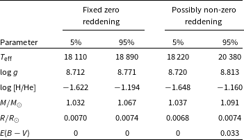
Two sets of 90% confidence intervals are given in Table 2, both calculated for the reddening-free model in the last line of Table 1. For the first set, the reddening was fixed at zero. For the second set of results, solutions with $E(B-V) \ne 0$
were allowed, even though the null model reddening was zero. Not surprisingly the confidence intervals for the first set of bootstrap results are narrower.
$E(B-V) \ne 0$
were allowed, even though the null model reddening was zero. Not surprisingly the confidence intervals for the first set of bootstrap results are narrower.
Percentage points defining 90% confidence intervals for the properties of Feige 7, as given in the last line of Table 1.
3. Previous time-series photometry
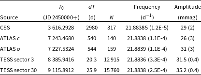
The position on the sky of Feige 7 has been covered by a number of large surveys which obtained measurements at different epochs. These include the ‘Catalina Sky Survey’ (CSS – Drake et al. 2014);Footnote e the ‘Asteroid Terrestrial-impact Last Alert System’ (ATLAS – e.g. Heinze et al. Reference Heinze, Tonry and Denneau2018);Footnote f the ‘Transiting Exoplanet Survey Satellite’ (TESS – Ricker et al. 2015);Footnote g and the ‘Near Earth Object Wide-field Infrared Survey Explorer’ (NEOWISE – Mainzer et al. Reference Mainzer, Bauer and Cutri2014).Footnote h (Note that the URLs are for the relevant data, rather than for the overall projects). The small amplitude of the variations of Feige 7 in the infrared meant that the variability could not be seen in the NEOWISE data, although it was possible to identify it in the other three sources.
Frequencies and amplitudes extracted from the data are in Table 3. Due to the double wave nature of the light curve, and the fact that the two halves are fairly similar, the values in the Table are double the true frequency of variation – the quality of the data are not sufficient to show the subharmonic. The time baseline of the CSS photometry is by far the longest, hence those data provide the best estimate of the frequency of variation. The amplitudes are similar, except for that found during the second TESS run, which is markedly larger than the rest.
Frequencies and semi-amplitudes extracted from various datasets. The ATLAS o (orange) and c (cyan) filters have bandpasses of 560–820 and 420–650 nm respectively. The second and third columns of the Table respectively contain the start time and duration of the sequences of observations. Standard errors on the frequencies and amplitudes are shown in brackets.
4. SAAO photometry
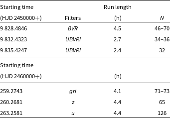
All the new measurements were made with the SAAO (South African Astronomical Observatory) SHOC CCD camera mounted on SAAO telescopes at Sutherland, South Africa. One set of observations were obtained using UBVRI filters, the a second set using ugriz filters. Typically measurements were made cycling through several filters, though the last two runs concentrated on single filters (z and u). Table 4 contains an observing log.
The observing log. All observations were made using the SAAO 1m telescope, except the runs on JD 2459832 and JD 2459835, which utilised the 1.9m telescope. The last column gives the number of observations across the different filters used during the particular run.
Photometric reductions were performed using an automated version of DOPHOT (Schechter, Mateo & Saha 1993). Magnitudes determined from point spread functions were used as these proved less noisy than those from aperture photometry. Differential corrections were applied to compensate for changing atmospheric conditions.
5. Analysis of the SAAO data
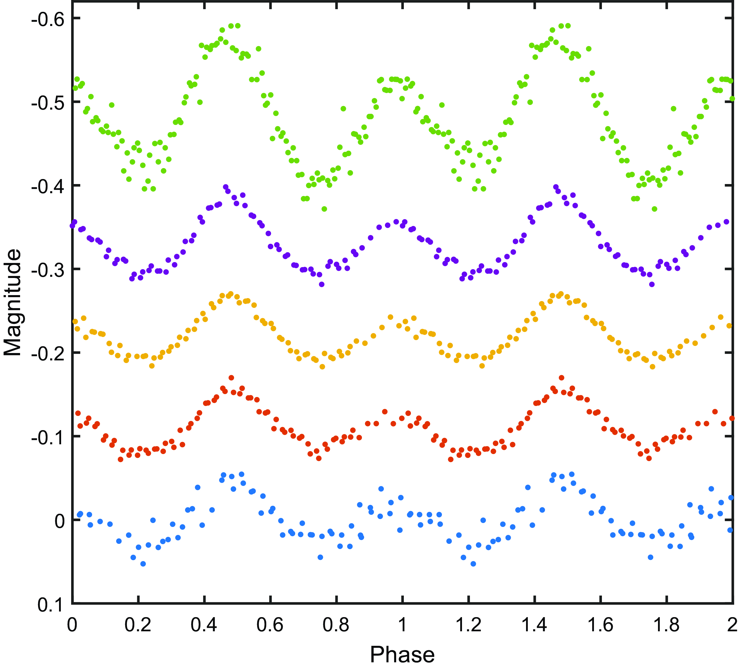
The phased light curves are plotted in Figs. 2 and 3. It is obvious that the amplitudes in U and u are larger by some margin. The peak-to-peak amplitudes can be objectively estimated by fitting truncated Fourier series of the form
 \begin{equation}Y(\phi)=\sum_{k=1}^K [\alpha_j \cos(2\pi k\phi)+\beta_j\sin(2\pi k \phi)]\end{equation}
to the phased data.
Phased SAAO Johnson-Cousins photometry, with U, B, V, R, I from top to bottom.
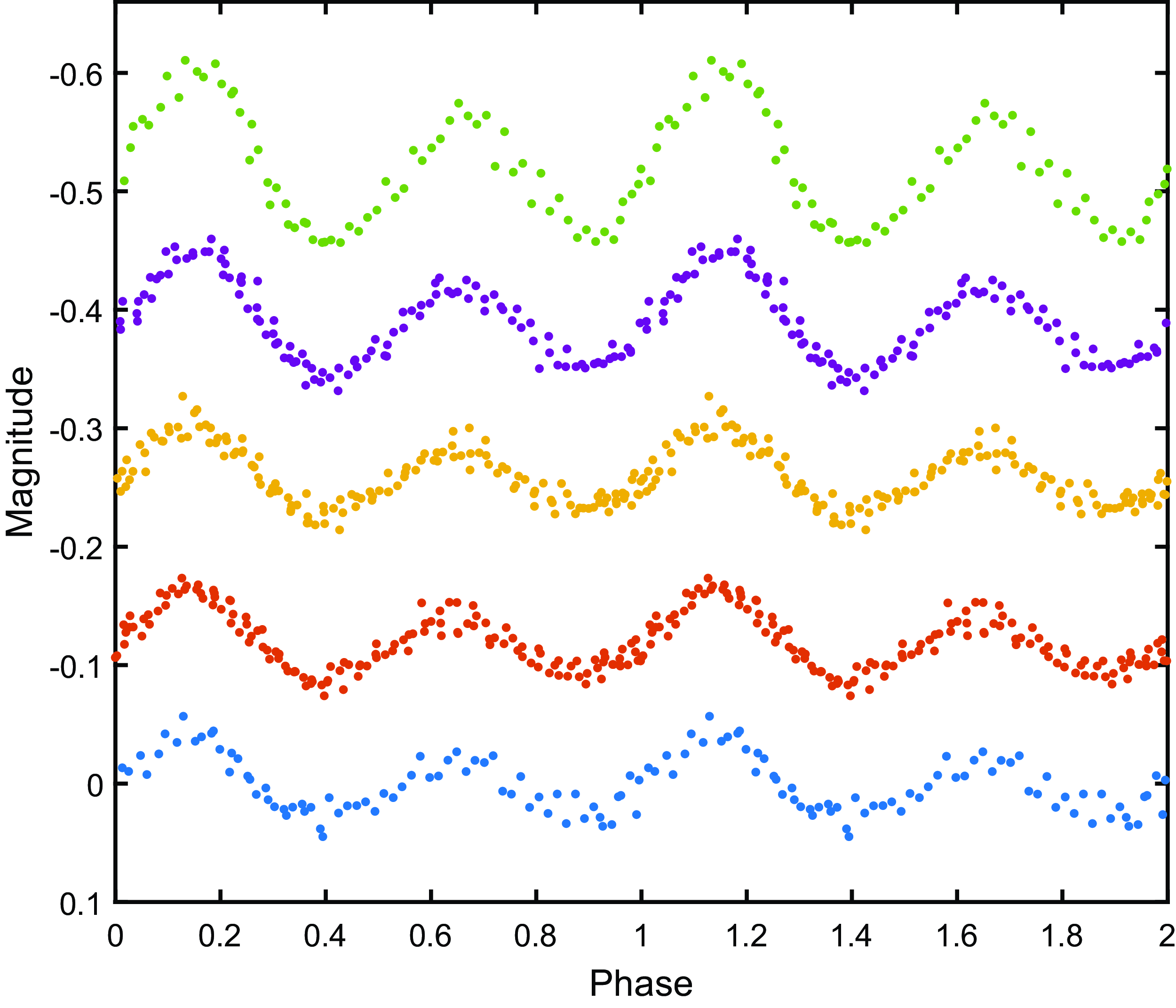
Phased SAAO Sloan filter photometry, with u, g, r, i, z from top to bottom.
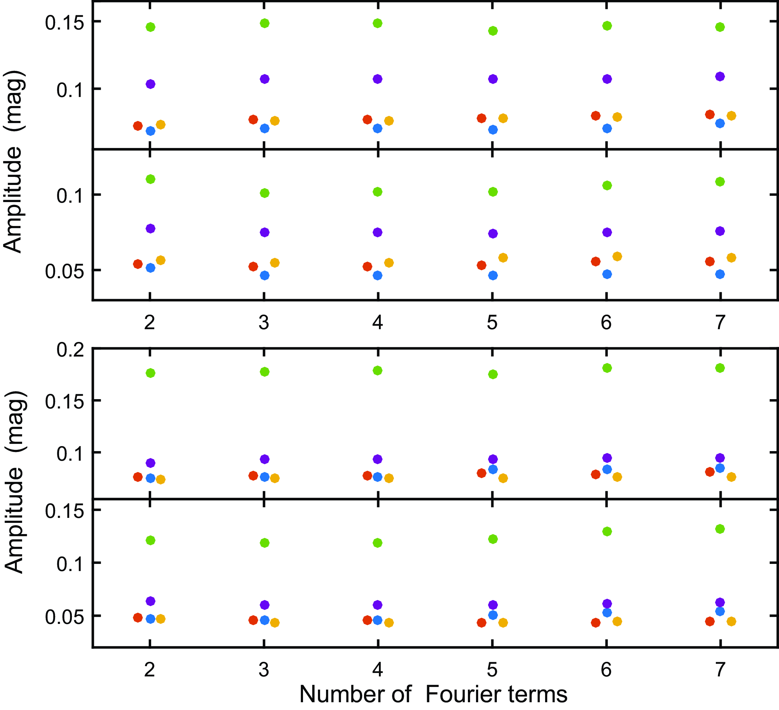
Measures such as the Akaike or Bayes information criteria (AIC or BIC – e.g. Burnham & Anderson 2002) can be used to select optimal values of K, but results are evidently not very sensitive to it – see Fig. 4. For most of the datasets, the typically more conservative BIC favours $2 \le K \le 5$
. The differences in K for different filters most likely reflects the effects of noise in the observations, rather than true differences in the shapes of the light curves. In order to accommodate the uncertainty, we proceed with average amplitudes over the range
$2 \le K \le 5$
. The differences in K for different filters most likely reflects the effects of noise in the observations, rather than true differences in the shapes of the light curves. In order to accommodate the uncertainty, we proceed with average amplitudes over the range $2 \le K \le 5$
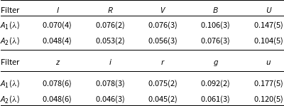
– see Table 5. Standard errors can be estimated by using bootstrapping for which we use a base model with
$2 \le K \le 5$
– see Table 5. Standard errors can be estimated by using bootstrapping for which we use a base model with $K=3$
.
$K=3$
.
The peak-to-peak amplitudes extracted from the light curves in Fig. 2 (top two panels) and Fig. 3 (bottom two panels), for a range of terms in the fitting function (Equation 1). The colour coding is the same as in Figs. 2 and 3, namely green for U, u; purple for B, g; orange for V, r; red for R, i; blue for I, z. The horisontal positions of the plotted points for R, i and V, r have been shifted slightly to avoid overplotting. Estimation errors are of the order of the symbol sizes or smaller – cf. Fig. 5.
The wavelength dependence of the amplitudes is plotted in Fig. 5, together with the estimated errors. Amplitudes appear to be roughly constant for wavelengths longer than 5000 Å.
We assume that the light curves are dominated by spots on either side of the star. The spots could be due to regions on the stellar surface with temperatures and/or compositions which differ from that of the undisturbed photosphere, which is assumed to be characterised by the parameters in the last line of Table 1. Formally, the following simple model is adopted:
 \begin{eqnarray}A_{j\lambda} &=& -2.5 \log F_{0\lambda}+2.5\log [(1-f)F_{0\lambda}+f F_{j\lambda}]\;\;\;\; j=1,2 \nonumber\\[5pt] &=& 2.5\log [1-f+f F_{j\lambda}/F_{0\lambda}]\end{eqnarray}
where j indexes the sets of amplitudes (1 for large, 2 for small), $\lambda$
indexes the filter,
$\lambda$
indexes the filter, $F_{0\lambda}$
is the undisturbed photospheric flux, and f is the spot filling factor (fraction of the hemisphere covered by the spot). The flux from spot j is denoted by
$F_{0\lambda}$
is the undisturbed photospheric flux, and f is the spot filling factor (fraction of the hemisphere covered by the spot). The flux from spot j is denoted by $F_{j\lambda}$
; this will be taken to equal the theoretical flux from a WD with slightly a different temperature and composition from that of the undisturbed photosphere. The flux ratio is given by
$F_{j\lambda}$
; this will be taken to equal the theoretical flux from a WD with slightly a different temperature and composition from that of the undisturbed photosphere. The flux ratio is given by
 \begin{equation}F_{j\lambda}/F_{0\lambda}= 10^{0.4 (m_{0\lambda}-m_{j\lambda})}\end{equation}
where $m_{0\lambda}$
and
$m_{0\lambda}$
and $m_{j\lambda}$
are magnitudes determined respectively by the parameters in the last line of Table 1, and by the unknown temperatures and compositions in the two spotted areas.
$m_{j\lambda}$
are magnitudes determined respectively by the parameters in the last line of Table 1, and by the unknown temperatures and compositions in the two spotted areas.
Peak-to-peak amplitudes (in magnitude units) of the two bumps in the Feige 7 light curves.
Peak-to-peak amplitudes for the two ‘bumps’ in the Feige 7 light curve, vs the filter effective wavelength (in the order uUBgVrRiIz). One sigma error bars are shown.

Equation (2) assumes bright spots; for dark spots, the right-hand side is multiplied by -1. Equations (2) and (3) can be solved by least squares, minimising the differences between the observed (left-hand side) and theoretical (right hand side) amplitudes in (2). Results are given in Table 6. As suggested by the residual standard deviations and confirmed by the Akaike and Bayes information criteria, the overall preferred model ascribes the variability as being due to cool spots caused by slightly (520 and 370 K) lower temperatures and higher Hydrogen content. The filling factors are quite large – 68% and 49% respectively. If the spots were bright, then composition changes would probably play a minor role, variability being dominated by tiny areas with very high temperatures.
Two remarks are in order: first, observationally hot spots with temperatures of 60 000–70 000 K can probably be ruled out due to the lack of emission lines in the spectra of Feige 7. Second, the abundance changes given in Table 6 are small compared with those derived by Achilleos et al. (Reference Achilleos, Wickramasinghe, Liebert, Saffer and Grauer1992) from detailed modelling of their high dispersion spectra.
The best hot and cool spot model predictions are compared to the observed amplitudes in Figs. 6 and 7. The fits of the two models are similar in quality for the low amplitude variation, but the cool spot model is clearly superior for the larger amplitudes.
Details of the simple starspot models fitted to the variability amplitudes given in Table 5. Index 1(2) in the first column refers to the larger(smaller) amplitude. For each amplitude, the first line reports spots with properties due to only a temperature difference; the second line, properties due to only a composition difference; and the third both a temperature and a composition difference. The gravity is fixed at log $\;g=8.74$
for all models. Columns 5 and 9 give the residual standard deviation.
$\;g=8.74$
for all models. Columns 5 and 9 give the residual standard deviation.

Theoretical amplitudes (circles) predicted by the optimal model which assumes that the variability in Feige 7 is due to two hot surface spots. The observations are denoted by the dots with error bars. The two panels are respectively for the large and small amplitudes in Fig. 5.

As for Fig. 6, but for the optimal cool spots model.

6. Discussion
Brinkworth et al. (2013) searched for photometric variability in 30 magnetic white dwarf stars with no overt signs of multiplicity. Fourteen of the stars were found to be variable. Of these, HE 1211-1707 has properties which are closest to those of Feige 7 – it is a DB WD, with a magnetic field of 50 MG and rotation period of 1.8 h. Its effective temperature is in the range 20 000–25 000 K (Reimers et al. 1996). Interestingly, Reding et al. (2018) found that the incidence of variability due to starspots is particularly low amongst white dwarfs with temperatures in the range 10 000–29 000 K.
As far as the origin of surface spots on magnetic WDs is concerned, there are several mechanisms which could give rise to bright spots (see e.g. the discussion in Maoz, Mazeh, & McQuillan Reference Maoz2014). Perhaps the most frequently cited is magnetic dichroism, i.e. variations in opacity across the stellar surface which are induced by the magnetic field (e.g. Ferrario et al. 1997; Maoz et al. Reference Maoz2014). Second, variations in magnetic pressure could give rise to areas of increased surface temperature on the star (Fendt & Dravins 2000; Reding, Hermes, & Clemens 2018, Momany et al. Reference Momany, Zaggia and Montalto2020). Third, magnetic field lines could funnel accretion from the interstellar medium onto magnetic poles (e.g. Maoz et al. Reference Maoz2014). If the variability in Feige 7 is caused by hot surface spots, accretion is the most probable mechanism, given the high temperatures and small filling factors (Table 6).
Dark surface spots are usually ascribed to magnetic inhibition of convection. In this context, it is noteworthy that the envelopes of DB WDs are convective at temperatures below about 23 000 K (e.g. Brinkworth et al. 2013), i.e. Feige 7 has a convective atmosphere. It is noteworthy that the optimal ‘cool spot’ models in Table 6 have Hydrogen abundances elevated above the average, which means that less Helium may have been brought to the surface in these areas (cf. the discussion in Section 1).
Finally, we note that none of the models accurately account for the sharp rise of the amplitudes in the near-ultraviolet u and U bands. It is conceivable that this excess high energy radiation could be due to non-thermal emission powered by the star’s magnetic field. Observations of the star at even shorter wavelengths would reveal whether the trend of steeply increasing amplitudes continues – this could set more stringent constraints on models.
Acknowledgements
Allocation of telescope time by the South African Astronomical Observatory and the smooth operation of the equipment are gratefully acknowledged. This research has made use of the Simbad database at CDS, Strasbourg, France. The authors are grateful for the public availability of the CSS, ZTF, and ATLAS photometry.
Data availability statement
SAAO photometry is available from the authors of this paper; other observations were downloaded from the websites mentioned.


 Open access

