


1. Introduction
As life expectancy rises globally, the strains on healthcare systems, pension schemes, and insurers have intensified. This intensification underscores the need to understand the different drivers of mortality improvement (see Booth and Tickle Reference Booth and Tickle2008; Basellini et al. Reference Basellini, Camarda and Booth2023, for comprehensive reviews). Modeling cause-of-death (COD) rates is essential to unravel the heterogeneity underlying aggregate longevity trends and identify their drivers. Early studies showed that most mortality improvements stemmed from declines in circulatory diseases, a finding obscured by all-cause forecasts alone (Keyfitz Reference Keyfitz1972; Manton and Stallard Reference Manton and Stallard1982). In life insurance, underwriting schemes often exclude high Cardiovascular risk, shifting the insured pool toward other causes such as cancer and accidents (Munich RE 2019). These considerations have driven the development of models for cause-specific mortality over the past few decades (see, e.g., McNown and Rogers Reference McNown and Rogers1992; Dimitrova et al. Reference Dimitrova, Haberman and Kaishev2013; Alai et al. Reference Alai, Arnold, Bajekal and Villegas2018; Li et al. Reference Li, Li, Lu and Panagiotelis2019; Li and Lu Reference Li and Lu2019; Li et al. Reference Li, Balasooriya and Liu2021, to name a few)
This paper proposes a holistic methodology for modeling COD rates with applications in out-of-sample forecasting and in-sample spillover analysis. The modeling framework is built on two key features highlighted in the literature. First, disaggregated mortality rates exhibit hierarchical dependency and require statistical reconciliation (see, e.g., Hyndman et al. Reference Hyndman, Ahmed, Athanasopoulos and Shang2011; Shang Reference Shang2017; Li et al. Reference Li, Li, Lu and Panagiotelis2019; Li and Chen Reference Li and Chen2024). Second, COD rates share long-term equilibrium relationships that must be respected in any coherent model (see, e.g., Arnold and Sherris Reference Arnold and Sherris2015; Arnold and Glushko Reference Arnold and Glushko2021; Arnold and Glushko Reference Arnold and Glushko2022).Footnote 1
For the first feature, efforts to address dependence and reconciliation in COD modeling have evolved. Early studies, including Manton and Stallard (Reference Manton and Stallard1982) and Janssen and Kunst (Reference Janssen and Kunst2007), assumed independence between cause-specific mortality rates. Although simple, this assumption overlooks the dependencies driven by shared risk factors, medical interventions, and demographic transitions. Later work tackled dependence in COD modeling in various ways: Alai et al. (Reference Alai, Arnold and Sherris2015) employed a multinomial logistic framework for competing risks; Lyu et al. (Reference Lyu, De Waegenaere and Melenberg2021) used multi-output Gaussian processes; and Dong et al. (Reference Dong, Shang, Hui and Bruhn2025) applied compositional data-analytic methods. These approaches often impose strong distributional assumptions. More importantly, they fail to comprehensively exploit the natural hierarchy in mortality data, where disaggregated death counts must sum to the aggregate total. Reconciliation methods leverage this hierarchy to ensure coherent forecasts across all levels. However, existing studies apply reconciliation only at the out-of-sample forecasting step (see, e.g., Shang Reference Shang2017; Li et al. Reference Li, Li, Lu and Panagiotelis2019; Li and Chen Reference Li and Chen2024). As in-sample lower-level mortality rates are modeled independently of reconciliation, this underuses hierarchical information. Given the scarcity of mortality data, neglecting useful in-sample information can inflate uncertainty and compromise forecast accuracy.
For the second feature, COD data are argued to present the long-run equilibrium relationships (Arnold and Sherris Reference Arnold and Sherris2015; Arnold and Glushko Reference Arnold and Glushko2021). As shown in Arnold and Glushko (Reference Arnold and Glushko2022), cancer, circulatory, and respiratory mortality share a common stochastic trend driven by biological aging and broad medical advances. Cointegration methods, such as the vector error correction model (VECM), are therefore essential to prevent divergent long-term forecasts for these co-moving rates and to improve model validity and interpretability. However, standard VECM approaches neither account for hierarchical dependence nor perform reconciliation across disaggregation levels. In addition, to manage the high dimensionality of age- and time-specific mortality data, VECMs are typically applied to age-standardized rates. Because standardization weights each age by a fixed population distribution, larger cohorts at younger ages dominate the aggregate series. This can distort the temporal patterns of cause-specific mortality, especially for diseases that predominantly affect older people.
Building on existing studies and addressing their limitations, we propose a holistic framework that integrates hierarchical dependence, in-sample reconciliation, and cointegration. To handle the high dimensionality of age–period data, we first apply Lee and Carter’s (Reference Lee and Carter1992) model, which decomposes logarithmic mortality rates into orthogonal age index ( $b_x$
) and period index (
$b_x$
) and period index ( $\kappa_t$
). This period index more accurately reflects the general temporal patterns of cause-specific mortality than age-standardized rates. To improve the Lee–Carter (LC) estimates, we further reconcile the fitted and observed death counts for each COD. Using these reconciled period indices, we follow Li et al. (Reference Li, Li, Lu and Panagiotelis2019) and consider three types of clustering analysis: dynamic time warping (DTW) clustering (Varga Reference Varga2025), slope clustering based on changes of
$\kappa_t$
). This period index more accurately reflects the general temporal patterns of cause-specific mortality than age-standardized rates. To improve the Lee–Carter (LC) estimates, we further reconcile the fitted and observed death counts for each COD. Using these reconciled period indices, we follow Li et al. (Reference Li, Li, Lu and Panagiotelis2019) and consider three types of clustering analysis: dynamic time warping (DTW) clustering (Varga Reference Varga2025), slope clustering based on changes of $\kappa_t$
, and trend polarity clustering. The different hierarchical trees are then identified and used to model COD dependence via a hierarchical Archimedean copula (HAC), as in Li and Lu (Reference Li and Lu2019) and Li et al. (Reference Li, Balasooriya and Liu2021). In addition, cointegration among the
$\kappa_t$
, and trend polarity clustering. The different hierarchical trees are then identified and used to model COD dependence via a hierarchical Archimedean copula (HAC), as in Li and Lu (Reference Li and Lu2019) and Li et al. (Reference Li, Balasooriya and Liu2021). In addition, cointegration among the $\kappa_t$
series is enforced through a sparse VECM, where the sparsity pattern is determined by the clustering-specific hierarchy as previously identified. Finally, to capture the potential conditional heteroskedasticity in each cause, we specify GARCH innovations (Lee and Miller Reference Lee and Miller2001; Lin et al. Reference Lin, Wang and Tsai2015; Zhou Reference Zhou2019).
$\kappa_t$
series is enforced through a sparse VECM, where the sparsity pattern is determined by the clustering-specific hierarchy as previously identified. Finally, to capture the potential conditional heteroskedasticity in each cause, we specify GARCH innovations (Lee and Miller Reference Lee and Miller2001; Lin et al. Reference Lin, Wang and Tsai2015; Zhou Reference Zhou2019).
To illustrate the usefulness of our model, we provide two applications. The first is out-of-sample forecasting of aggregate mortality rates, a central task in actuarial science and demographic forecasting. For each clustering strategy, a sparse VECM with HAC dependence and GARCH errors is estimated for the COD series. The aggregate rate is then forecast using a bottom-up reconciliation of the predicted COD rates, consistent with approaches in existing studies such as Shang (Reference Shang2017) and Li and Chen (Reference Li and Chen2024). As explained above, our framework fully exploits information across all COD series, including reconciliation, hierarchical dependence, long-run equilibrium, and heteroskedasticity. Hence, it is expected to deliver superior forecasting performance relative to standard benchmarks such as the LC model.
The second application is in-sample structural analysis, which reveals spillovers and interdependence among COD trends. Structural tools such as impulse response functions (IRFs) are common in economics and finance studies (Mensi et al. Reference Mensi, Al-Yahyaee, Vo and Kang2021; Wan and He Reference Wan and He2021), but have only recently been applied in mortality research. For example, Arnold and Glushko (Reference Arnold and Glushko2022) showed that shocks to circulatory and cancer mortality primarily transmit to respiratory and infectious/parasitic causes, with short-lived effects. Shi et al. (Reference Shi, Shi, Wang and Zhu2024) found pronounced cross-country responses to U.S. shocks in G7 data. However, these studies rely solely on traditional IRFs, which are limited in their ability to quantify the relative importance of shocks to individual variables or to capture the broader network of spillovers. To overcome these limitations, we adopt the connectedness measure of Diebold and Yilmaz (Reference Diebold and Yilmaz2012). The connectedness employs generalized forecast-error variance decompositions (FEVDs) to derive intuitive directional spillover measures and thus provides a comprehensive view of interdependencies among COD trends.
Our empirical dataset comprises U.S. male COD rates from 1970 to 2018, by single-year ages 1–85+. Following Li et al. (Reference Li, Li, Lu and Panagiotelis2019), we focus on seven causes: cancer, diabetes, external causes, influenza, mental disorders, nephritis, and vascular disease. To evaluate out-of-sample forecasting performance, we split the data into a training period (1970–2008) and a test period (2009–2018). For each clustering method, the Gumbel HAC copula is selected based on the training set. We then apply the fitted sparse-VECM–GARCH–Gumbel-HAC model to forecast the test period. Although all clustering-based models outperform the standard LC benchmark, trend-polarity clustering, which groups causes into increasing (diabetes, mental disorders, and nephritis) and declining (cancer, external causes, influenza, and vascular) trends, yields the best accuracy. This result remains robust in the sensitivity analysis that shift the training start year to 1980, extend the test period to 2004–2018, and aggregate ages into five-year bands. For the in-sample application, using this best-performing model for the entire 1970–2018 sample, we computed the connectedness. Our results show that diabetes, nephritis, and vascular disease act as net transmitters of mortality shocks, while cancer and external causes remain largely self-contained net receivers.
The contributions of this paper are threefold with the scope of U.S. male data: We are among the first to introduce a holistic framework that jointly accommodates hierarchical reconciliation and cointegration in the modeling of mortality from COD. By embedding penalized reconciliation into the LC estimation of COD period indices, the accuracy of the parameter estimates in the sample is improved. With sparse VECM and HAC, we incorporate hierarchical short-run interactions, tail dependence, and long-run equilibrium among COD trends. Our empirical evaluation demonstrates the superiority of the sparse-VECM–GARCH–Gumbel-HAC model. By integrating all COD mortality information, our model consistently outperforms the LC model. Hence, the proposed holistic framework can be extended to enhance mortality forecasting by leveraging additional hierarchical information, such as regional or sub-population-level factors (e.g., socioeconomics or ethnic groups). This paper is the first to study the connectedness among COD trends. Our findings have important implications in practice. Clinically and for public health policy suggest the potential value of prioritizing interventions for high-transmission conditions (e.g., through integrated care for hyperglycemia, hypertension, and renal dysfunction) to disrupt comorbidity cascades and maximize population-level mortality improvements.
The remainder of this paper is organized as follows. Section 2 introduces the motivating data. Section 3 presents the LC model. Section 4 describes the clustering analysis. Section 5 details the complete modeling framework. Section 6 outlines the forecasting procedure and presents the results. Section 7 performs the structural connectedness analysis. Section 8 concludes the paper, along with some ideas on how the methodology presented can be further extended.
2. Cause-specific mortality data
We analyze male cause-specific mortality rates in the U.S., denoted by $m_{i,t}(x)$
, for single-year ages
$m_{i,t}(x)$
, for single-year ages $x=1,\dots,85+$
during the 1970–2018 period. For each cause i, we compute the mortality rates for each age and year as the number of deaths divided by the population at risk.
$x=1,\dots,85+$
during the 1970–2018 period. For each cause i, we compute the mortality rates for each age and year as the number of deaths divided by the population at risk.
Population exposures by age and calendar year were drawn from the Surveillance, Epidemiology, and End Results (SEER) database (Surveillance, Epidemiology, and End Results (SEER) Program Reference Surveillance and Results2025) using its accompanying data dictionary (National Center for Health Statistics (NCHS) 2025). Annual cause-specific death counts for ages 1–85+ were obtained from the Centers for Disease Control and Prevention (CDC) mortality files, accessed through the National Bureau of Economic Research website (National Bureau of Economic Research (NBER) 2023). CDC data include individual-level records of date of birth, sex, age at death, and underlying cause of death (UCOD), coded according to the International Classification of Diseases (ICD). The National Center for Health Statistics later recoded roughly 1000 ICD categories into broader groups for public release.Footnote 2
To construct a series of consistent cause-specific death counts from 1970 to 2018, we harmonize the codes of the International Classification of Diseases, Eighth Revision (ICD-8; 1970–1978), Ninth Revision (ICD-9; 1979–1998), and Tenth Revision (ICD-10; 1999–2018) following the framework of Li et al. (Reference Li, Li, Lu and Panagiotelis2019). Seven major causes of death groups are defined by the UCOD codes;Footnote 3 refer to Table 1 for the complete mapping.Footnote 4 For example, neoplasms are identified by UCOD 050–110 under ICD-8, UCOD 50–110 under ICD-9, and UCOD 004–015 under ICD-10. This alignment produces a consistent time series of Cancer mortality in all three revisions of the ICD.
Cause-of-death coding across ICD revisions (1970–2018).

Figure 1 shows the log of the seven-cause total mortality ratesFootnote 5 for U.S. males from 1970 to 2018. The curves indicate a sustained decline in mortality over time. Across ages, the logarithm of the mortality rate falls sharply from age 1 to 10, reflecting reductions in infant and early childhood mortality. An apparent increase between 20 and 30 years potentially corresponds to increased deaths from external causes (e.g., accidents and violence). At older ages, the curves converge, illustrating mortality compression: variability in mortality rates among the elderly decreases over time. In general, improvements in mortality are most pronounced in younger ages, while rates at older ages change more gradually.
The natural logarithm of death rates for seven-cause total mortality.

We present rainbow plots of age-specific logarithmic mortality for the seven COD groups defined in this study. Refer to Figure S.1 in the Supplementary Materials for details. These plots reveal distinctive age patterns and temporal trends among COD groups. However, such distinctions are obscured when all causes are aggregated into the total mortality rate, as shown above.
Remark 1. This finding yields two key insights. First, although individual cause-specific rates follow divergent temporal trajectories, they may co-move when combined in a weighted sum (i.e., total rates).Footnote 6 Second, the prediction of total mortality could be improved by explicitly modeling the temporal dynamics of each cause-specific rate with appropriate reconciliation.
Inspired by the framework of Li et al. (Reference Li, Li, Lu and Panagiotelis2019), this study develops a three-stage holistic approach to modeling the COD mortality rates. First, each COD mortality rate is decomposed into orthogonal age-specific and temporal components. Second, various clustering strategies are applied to the seven COD-based temporal indices to reduce dimensionality and uncover latent group structures. Third, a comprehensive econometric model is estimated, incorporating cluster-level short-run dependence and long-run equilibrium, as highlighted in Remark 1. To enhance accuracy, the estimation also integrates reconciliation for the fitted death counts, hierarchical Archimedean copula dependence, and heteroskedasticity for the innovations. Sections 3–5 examine each stage in detail.
3. Lee–Carter method for modeling baseline cause-of-death
Following Li et al. (Reference Li, Li, Lu and Panagiotelis2019), we adopt the LC model (Lee and Carter Reference Lee and Carter1992) to decompose and characterize each COD mortality rate. For cause i, single-year of age x, and calendar year t, the log mortality rate is modeled by
 \begin{equation}\ln m_{i,t}(x) = a_i(x) + b_i(x)\,\kappa_{i,t} + \epsilon_{i,t}(x),\end{equation}
where
 \begin{equation*}m_{i,t}(x)=\frac{D_{i,t}(x)}{E_t(x)},\end{equation*}
with $D_{i,t}(x)$
is the number of deaths and
$D_{i,t}(x)$
is the number of deaths and $E_t(x)$
is the central exposed-to-risk for all causes. In (3.1),
$E_t(x)$
is the central exposed-to-risk for all causes. In (3.1), $a_i(x)$
is the baseline age profile,
$a_i(x)$
is the baseline age profile, $b_i(x)$
measures the age-specific sensitivity to temporal changes,
$b_i(x)$
measures the age-specific sensitivity to temporal changes, $\kappa_{i,t}$
is the period index, and
$\kappa_{i,t}$
is the period index, and $\epsilon_{i,t}(x)$
is the error term, assumed to follow a multivariate Gaussian distribution.
$\epsilon_{i,t}(x)$
is the error term, assumed to follow a multivariate Gaussian distribution.
We estimate $\{a_i(x),b_i(x),\kappa_{i,t}\}$
by applying singular value decomposition (SVD). In Figure 2, we display these parameter estimates by separately fitting each COD log mortality rate.
$\{a_i(x),b_i(x),\kappa_{i,t}\}$
by applying singular value decomposition (SVD). In Figure 2, we display these parameter estimates by separately fitting each COD log mortality rate.
LC original parameter estimates for different causes of death.

The estimated baseline function $a_i(x)$
increases almost monotonically with age for all causes, reflecting the well-known growth in mortality at older ages. The external causes show a pronounced secondary peak between 20 and 30, corresponding to the “accident hump”. Consistent with our observations in Figure S.1, the period index
$a_i(x)$
increases almost monotonically with age for all causes, reflecting the well-known growth in mortality at older ages. The external causes show a pronounced secondary peak between 20 and 30, corresponding to the “accident hump”. Consistent with our observations in Figure S.1, the period index $\kappa_{i,t}$
declines for cancer, external causes, influenza, and vascular diseases, indicating improvements in mortality for these causes. In contrast,
$\kappa_{i,t}$
declines for cancer, external causes, influenza, and vascular diseases, indicating improvements in mortality for these causes. In contrast, $\kappa_{i,t}$
increases for diabetes and mental disorders, indicating worsening trends. The age sensitivity parameter
$\kappa_{i,t}$
increases for diabetes and mental disorders, indicating worsening trends. The age sensitivity parameter $b_i(x)$
also varies by cause: for mental disorders,
$b_i(x)$
also varies by cause: for mental disorders, $b_i(x)$
increases sharply at advanced ages, highlighting increased vulnerability to mortality among the elderly; while for cancer, external causes, and influenza,
$b_i(x)$
increases sharply at advanced ages, highlighting increased vulnerability to mortality among the elderly; while for cancer, external causes, and influenza, $b_i(x)$
decreases with age, implying that relative mortality improvements are smaller at older ages.
$b_i(x)$
decreases with age, implying that relative mortality improvements are smaller at older ages.
It is worth noting that the temporal pattern of nephritis is deemed declining under the original LC model. However, this result conflicts with the empirical evidence. As shown in Figure 3, the log mortality rate of nephritis, aggregated over all ages, exhibits a clear upward trend. The discrepancy underscores the limitation of the original LC model in capturing the actual temporal dynamics of nephritis when modeled in isolation without appropriate adjustment. Consequently, applying clustering analysis directly to temporal indices derived from the uncorrected LC model may yield inefficient or misleading cluster structures. $\log_e$
of total annual mortality rates of Nephritis.
$\log_e$
of total annual mortality rates of Nephritis.

To address this, we explore how these inconsistencies could be corrected by leveraging reconciliation for each COD rate. The technical details are presented in Section 2 of the Supplementary Materials. Figure 4 plots the estimated parameters of the LC method with correction. Compared to the fitted $\kappa_t$
’s in Figure 2, the temporal index of nephritis is consistent with the increasing trend shown in Figure 3 and is more reliable. For their improved accuracy, the corrected LC parameters will be used for subsequent analyses.
$\kappa_t$
’s in Figure 2, the temporal index of nephritis is consistent with the increasing trend shown in Figure 3 and is more reliable. For their improved accuracy, the corrected LC parameters will be used for subsequent analyses.
4. Clustering analysis
In the mortality literature, it is well known that mortality rates are subject to the curse of dimensionality due to data scarcity (see, e.g., Hyndman and Ullah Reference Hyndman and Ullah2007; Hyndman and Booth Reference Hyndman and Booth2008; Gao et al. Reference Gao, Shang and Yang2019, among others). To reduce the dimensionality of the COD rates, Li et al. (Reference Li, Li, Lu and Panagiotelis2019) used a data-driven clustering analysis to identify groups that reflect genuine temporal similarity among COD rates.
4.1. Hierarchical clustering with the dynamic time warping
Li et al. (Reference Li, Li, Lu and Panagiotelis2019) applied Ward’s hierarchical clustering to normalized age-specific COD mortality rates to identify hierarchical groupings. However, clustering directly on age-specific mortality rates can be inefficient. COD rates are often volatile and noisy, particularly at ages with small case-specific death counts. Hence, clustering such data does not effectively reduce this noise. Moreover, without decomposition, clustering on age–period matrices conflates age and period effects, making interpretation difficult. Finally, Ward’s method employs the Frobenius norm distance, which implicitly weights each dimension by its raw variance. As a result, even after normalization, dimensions with larger fluctuations may dominate, obscuring more interpretable clustering structures.
Remark 2. It is important to clarify that our use of the term “hierarchical” refers to the tree-structured grouping of cause-specific mortality trends derived from clustering algorithms. This structure dictates the nesting order for the Archimedean copulas and the sparsity constraints in the VECM. This is distinct from the “hierarchical” or “multilevel” terminology often employed in regression frameworks (e.g., linear mixed-effects models) to denote random effects nested within subjects or groups.
LC-corrected parameter estimates for different causes of death.

To resolve these issues, we follow Varga (Reference Varga2025) and perform the dynamic time warping (DTW) method to obtain hierarchical clusters to $b_i(x)$
and
$b_i(x)$
and $\kappa_{i,t}$
obtained as in Section 2 of the Supplementary Material. DTW is a shape-based distance measure originally developed by Bellman and Kalaba (Reference Bellman and Kalaba1959) for speech recognition applications. It computes an improved alignment between two time-series by allowing nonlinear “warping” along the time axis. In our context, taking
$\kappa_{i,t}$
obtained as in Section 2 of the Supplementary Material. DTW is a shape-based distance measure originally developed by Bellman and Kalaba (Reference Bellman and Kalaba1959) for speech recognition applications. It computes an improved alignment between two time-series by allowing nonlinear “warping” along the time axis. In our context, taking $\kappa$
’s as an example, DTW seeks a warping path
$\kappa$
’s as an example, DTW seeks a warping path $\psi = \{(h_1,v_1), \dots, (h_L,v_L)\}$
through the grid
$\psi = \{(h_1,v_1), \dots, (h_L,v_L)\}$
through the grid $\{1, 2, \dots,T\}^2$
that aligns each year h of
$\{1, 2, \dots,T\}^2$
that aligns each year h of $\kappa_{i,\cdot}$
with a (possibly different) year v of
$\kappa_{i,\cdot}$
with a (possibly different) year v of $\kappa_{j,\cdot}$
.
$\kappa_{j,\cdot}$
.
To build this alignment, we follow Varga (Reference Varga2025) and form the local cost matrix (LCM) using the $l_2$
norm:
$l_2$
norm:
 \begin{equation*}\mathrm{LCM}_{h,v}^\kappa\;=\;\bigl(\kappa_{i,h}^* - \kappa_{j,v}^*\bigr)^2,\end{equation*}
where $\kappa_{i,h}^*$
and
$\kappa_{i,h}^*$
and $\kappa_{j,v}^*$
are normalized entries from
$\kappa_{j,v}^*$
are normalized entries from $\kappa_{i,t}$
and
$\kappa_{i,t}$
and $\kappa_{j,t}$
, respectively. Each pair measures the pointwise discrepancy between the year h of one series and the year v of the other.
$\kappa_{j,t}$
, respectively. Each pair measures the pointwise discrepancy between the year h of one series and the year v of the other.
The DTW distance is then defined as the minimal cost route through this matrix. Let $\psi$
be any admissible path from (1, 1) to (T, T). Assign to each step
$\psi$
be any admissible path from (1, 1) to (T, T). Assign to each step $(h_\ell,v_\ell)\in\psi$
a weight
$(h_\ell,v_\ell)\in\psi$
a weight $\eta_\ell$
(set to unity) and let
$\eta_\ell$
(set to unity) and let $\eta = \sum_{\ell=1}^{L} \eta_\ell$
, where L is the length of the warping path
$\eta = \sum_{\ell=1}^{L} \eta_\ell$
, where L is the length of the warping path $\psi$
. The DTW distance is
$\psi$
. The DTW distance is
 \begin{equation*}{d}_{i,j}^\kappa\;=\;\min_{\psi}\Biggl\{\sum_{\ell=1}^L\frac{\eta_\ell \,\mathrm{LCM}_{(h_\ell,v_\ell)}}{\eta}\Biggr\}^{1/2}.\end{equation*}
This construction guarantees that the first and last years match exactly, while intermediate years can “stretch” or “compress” to reveal the strongest common trends, even if the improvement of one cause leads or lags the other.
To equally weight age and temporal dynamics in the cluster analysis, we define a composite DTW distance between two causes i and j as the sum of the univariate DTW distances. That is,
 \begin{equation*}{d}_{i,j}={d}_{i,j}^b+{d}_{i,j}^\kappa.\end{equation*}
The resulting DTW distance matrix can be computed via dynamic programming as in Giorgino (Reference Giorgino2009). This matrix is then used as input to the hierarchical clustering as in Sardá-Espinosa (Reference Sardá-Espinosa2019). The final clusters are plotted in Figure 5 and described in Table 2.
Clusters and hierarchical levels by clustering approach. The slope and trend-polarity clusterings are introduced in Section 4.2

Note: CA = cancer, DM = diabetes, EC = external causes, Flu = influenza, MD = mental disorder, NE = nephritis, VA = vascular disease.
Remark 3. Using DTW-based clustering on corrected LC parameters $b_i(x)$
and
$b_i(x)$
and $\kappa_{i,t}$
, we effectively address the potential problems of clustering analysis in Li et al. (Reference Li, Li, Lu and Panagiotelis2019). First, through parismonious LC decomposition, the dimensionality falls from
$\kappa_{i,t}$
, we effectively address the potential problems of clustering analysis in Li et al. (Reference Li, Li, Lu and Panagiotelis2019). First, through parismonious LC decomposition, the dimensionality falls from $N\times T$
to
$N\times T$
to $N+T$
. This drastic reduction filters out the large idiosyncratic volatility arising from small death counts at individual ages. Hence, the final clusters are driven by systematic demographic similarity rather than noise. Second, because
$N+T$
. This drastic reduction filters out the large idiosyncratic volatility arising from small death counts at individual ages. Hence, the final clusters are driven by systematic demographic similarity rather than noise. Second, because $b_i(x)$
and
$b_i(x)$
and $\kappa_{i,t}$
are treated separately, the age pattern and the temporal information remain disentangled. That is, DTW aligns time-series shapes in principal component score
$\kappa_{i,t}$
are treated separately, the age pattern and the temporal information remain disentangled. That is, DTW aligns time-series shapes in principal component score $\boldsymbol{\kappa}$
’s without conflating them with age effects, and clustering on principal component
$\boldsymbol{\kappa}$
’s without conflating them with age effects, and clustering on principal component $\boldsymbol{b}$
’s captures distinct age profiles. Finally, our distance metric explicitly balances the contributions of
$\boldsymbol{b}$
’s captures distinct age profiles. Finally, our distance metric explicitly balances the contributions of $\boldsymbol{b}$
’s and
$\boldsymbol{b}$
’s and $\boldsymbol{\kappa}$
’s by normalizing and weighting each component equally before applying DTW. This eliminates the implicit variance-driven dominance inherent in a Frobenius norm on the full age-time matrix. Thus, it ensures that the highly variable or more stable dimensions do not overshadow the demographic patterns of interest in the clustering analysis.
$\boldsymbol{\kappa}$
’s by normalizing and weighting each component equally before applying DTW. This eliminates the implicit variance-driven dominance inherent in a Frobenius norm on the full age-time matrix. Thus, it ensures that the highly variable or more stable dimensions do not overshadow the demographic patterns of interest in the clustering analysis.
The DTW-based clustering analysis reveals two primary hierarchical groups. The first cluster – diabetes, mental disorders, and nephritis – exhibits increasing trends in their $\kappa$
indices (Figure 3). The second cluster – vascular diseases, cancer, and external causes – demonstrates steady improvements over time, as shown in Figure 3. Within the first cluster, mental disorders and nephritis form the closest subcluster, while in the second cluster, cancer and external causes are identified as the closest pair. These groups align with the similarities observed in their estimated
$\kappa$
indices (Figure 3). The second cluster – vascular diseases, cancer, and external causes – demonstrates steady improvements over time, as shown in Figure 3. Within the first cluster, mental disorders and nephritis form the closest subcluster, while in the second cluster, cancer and external causes are identified as the closest pair. These groups align with the similarities observed in their estimated $b_i(x)$
and
$b_i(x)$
and $\kappa_{i,t}$
profiles (Figure 3). This underscores the effectiveness of our DTW-based method in capturing shared mortality dynamics.
$\kappa_{i,t}$
profiles (Figure 3). This underscores the effectiveness of our DTW-based method in capturing shared mortality dynamics.
Sample mean of $\triangle\kappa_{i,t}$
for each COD.
$\triangle\kappa_{i,t}$
for each COD.

Hierarchical clustering using custom DTW distance.

4.2. Alternative hierarchical clustering
In addition to the clusters identified in Figure 5, this section examines alternative clustering strategies. Unlike the DTW approach, which incorporates both age and temporal dimensions, the first alternative clustering method considers only the similarity of temporal dynamics.
Specifically, we computed the sample mean of the differenced $\kappa_{i,t}$
(i.e.,
$\kappa_{i,t}$
(i.e., $\triangle\kappa_{i,t} = \kappa_{i,t} - \kappa_{i,t-1}$
) using the corrected LC estimates. These means, shown in Table 3, represent the average annual rate of change in the period index. Consistent with the DTW results, two broad clusters emerge: one with positive mean values (indicating increasing trends) and one with negative mean values (indicating declining trends). Within the former, diabetes (0.23) and mental disorders (0.20) show the closest mean rates. Within the latter, cancer and external causes share similar means around
$\triangle\kappa_{i,t} = \kappa_{i,t} - \kappa_{i,t-1}$
) using the corrected LC estimates. These means, shown in Table 3, represent the average annual rate of change in the period index. Consistent with the DTW results, two broad clusters emerge: one with positive mean values (indicating increasing trends) and one with negative mean values (indicating declining trends). Within the former, diabetes (0.23) and mental disorders (0.20) show the closest mean rates. Within the latter, cancer and external causes share similar means around $-1$
, while influenza and vascular diseases form a sub-cluster with means roughly between
$-1$
, while influenza and vascular diseases form a sub-cluster with means roughly between $-2$
and
$-2$
and $-3$
. Based on these similarities, we construct the resulting hierarchical structure, shown in Table 2 (named slope clustering).
$-3$
. Based on these similarities, we construct the resulting hierarchical structure, shown in Table 2 (named slope clustering).
Finally, we consider a simplified clustering strategy that leverages only the overall trend. Two groups are identified: the first comprises causes exhibiting exclusively upward trends (diabetes, mental disorders, and nephritis), and the second includes those with downward mortality trends (cancer, influenza, external causes, and vascular diseases). No further hierarchical levels are defined. This two-tier structure (named trend-polarity clustering), together with the more granular cluster configurations explained above, is presented in Table 2 (named trend-polarity clustering).
5. Modeling framework
Using a pre-identified clustering structure, this section describes our modeling framework for COD log mortality rates, based on classical maximum likelihood estimation (MLE). First, we re-estimate the LC parameters within each cluster, imposing a cluster-dependent reconciliation penalty. Next, we model the re-estimated temporal indices $\kappa_{i,t}$
using a sparse VECM, or vector error correction model, augmented with GARCH innovations to capture both long-run equilibrium relationships and conditional heteroskedasticity. Finally, we specify cross-cause dependencies via a hierarchical Archimedean copula (HAC), thus completing the joint likelihood specification and enabling the full MLE.
$\kappa_{i,t}$
using a sparse VECM, or vector error correction model, augmented with GARCH innovations to capture both long-run equilibrium relationships and conditional heteroskedasticity. Finally, we specify cross-cause dependencies via a hierarchical Archimedean copula (HAC), thus completing the joint likelihood specification and enabling the full MLE.
5.1. Re-estimated LC parameters with cluster-dependent reconciliation
In Section 2 of the Supplementary Materials, corrected LC parameters were introduced to incorporate reconciliation information at the COD level. This correction improved estimation accuracy, which is essential for the clustering analysis in Section 4.1. Building on this, we propose a more flexible cluster-level reconciliation, which relaxes the requirement that fitted death counts match empirical counts for each COD.
For Cluster 2 identified by the DTW method (Figure 5), reconciliation proceeds sequentially:
-
(1) Bottom-level reconciliation. Apply a penalty term to reconcile fitted and empirical death counts for cancer and external causes.
-
(2) Intermediate-level reconciliation. Carry any remaining discrepancy from step (1) to reconcile vascular diseases alongside their own empirical and fitted death counts.
-
(3) Top-level reconciliation. Reconcile the residual difference from step (2) with the empirical and fitted death counts for Influenza.
A similar sequential reconciliation is performed independently for Cluster 1. Within each cluster, reconciliation at a higher aggregation level incorporates discrepancies from all subordinate levels, whereas reconciliation at a lower level does not incorporate information at higher levels.
Remark 4. In a hierarchical framework, each cluster-level series is, by definition, the aggregation of its constituent COD series. Hence, any misfit at the leaf (lower) level propagates naturally to its parent node (higher level). By reconciling the bottom-level CODs first, we ensure that the most similar mortality features are aligned before rolling to broader groupings. This bottom-up procedure adheres to the logic of hierarchical clustering: adjustments at lower levels drive the aggregation at higher levels, but not vice versa.
To improve accuracy, the LC parameters are re-estimated using the sequential and cluster-level reconciliation procedure described above. Taking the clusters identified by the DTW method as an example, we proceed as follows:
-
(1) At the bottom level, LC parameters for mental disorders and nephritis in Cluster 1 are re-estimated by solving
where \begin{equation*}\min_{a,b,\kappa}\;\sum_{i\in\{\mathrm{MD}, \mathrm{NE}\}}\sum_{x}\sum_{t}\bigl(\ln m_{i,t}(x) - [\,a_i(x) + b_i(x)\,\kappa_{i,t}\,]\bigr)^{2}\;+\;\lambda_{1,1}\sum_{i\in\{\mathrm{MD}, \mathrm{NE}\}}\sum_{x}\sum_{t}\bigl(D_{i,t}(x) - \widehat D_{i,t}(x)\bigr)^{2},\end{equation*}
$\lambda_{1,1}$
is a cluster- and level-specific penalty that enforces coherence and captures shared structure among causes grouped within Cluster 1 at Level 1 of the hierarchy. Similarly, the parameters for cancer and external causes in Cluster 2 are re-estimated by solving
\begin{equation*}\min_{a,b,\kappa}\;\sum_{i\in\{\mathrm{CA}, \mathrm{EC}\}}\sum_{x}\sum_{t}\bigl(\ln m_{i,t}(x) - [\,a_i(x) + b_i(x)\,\kappa_{i,t}\,]\bigr)^{2}\;+\;\lambda_{2,1}\sum_{i\in\{\mathrm{CA}, \mathrm{EC}\}}\sum_{x}\sum_{t}\bigl(D_{i,t}(x) - \widehat D_{i,t}(x)\bigr)^{2}.\end{equation*}
\begin{equation*}\min_{a,b,\kappa}\;\sum_{i\in\{\mathrm{MD}, \mathrm{NE}\}}\sum_{x}\sum_{t}\bigl(\ln m_{i,t}(x) - [\,a_i(x) + b_i(x)\,\kappa_{i,t}\,]\bigr)^{2}\;+\;\lambda_{1,1}\sum_{i\in\{\mathrm{MD}, \mathrm{NE}\}}\sum_{x}\sum_{t}\bigl(D_{i,t}(x) - \widehat D_{i,t}(x)\bigr)^{2},\end{equation*}
$\lambda_{1,1}$
is a cluster- and level-specific penalty that enforces coherence and captures shared structure among causes grouped within Cluster 1 at Level 1 of the hierarchy. Similarly, the parameters for cancer and external causes in Cluster 2 are re-estimated by solving
\begin{equation*}\min_{a,b,\kappa}\;\sum_{i\in\{\mathrm{CA}, \mathrm{EC}\}}\sum_{x}\sum_{t}\bigl(\ln m_{i,t}(x) - [\,a_i(x) + b_i(x)\,\kappa_{i,t}\,]\bigr)^{2}\;+\;\lambda_{2,1}\sum_{i\in\{\mathrm{CA}, \mathrm{EC}\}}\sum_{x}\sum_{t}\bigl(D_{i,t}(x) - \widehat D_{i,t}(x)\bigr)^{2}.\end{equation*}
-
(2) Define the remaining imbalance for each cluster by
\begin{align*}R_{1,1,t}(x) &= \sum_{i\in\{M,N\}}\bigl[D_{i,t}(x)-\widehat D_{i,t}(x)\bigr],\\[3pt]R_{2,1,t}(x) &= \sum_{i\in\{C,E\}}\bigl[D_{i,t}(x)-\widehat D_{i,t}(x)\bigr].\end{align*}
Then, the parameters for diabetes in Cluster 1 are re-estimated by solving
and the parameters for vascular diseases in Cluster 2 are re-estimated by solving
\begin{equation*}\min_{a,b,\kappa}\;\sum_{t,x}\bigl(\ln m_{\mathrm{DM}, t}(x) - [\,a_\mathrm{DM}(x) + b_\mathrm{DM}(x)\,\kappa_{\mathrm{DM}, t}\,]\bigr)^{2}\;+\;\lambda_{1,2}\sum_{t,x}\bigl(D_{\mathrm{DM}, t}(x) - \widehat D_{\mathrm{DM}, t}(x) - R_{1,1,t}(x)\bigr)^{2},\end{equation*}
\begin{equation*}\min_{a,b,\kappa}\;\sum_{t,x}\bigl(\ln m_{\mathrm{VA}, t}(x) - [\,a_\mathrm{VA}(x) + b_\mathrm{VA}(x)\,\kappa_{\mathrm{VA}, t}\,]\bigr)^{2}\;+\;\lambda_{2,2}\sum_{t,x}\bigl(D_{\mathrm{VA}, t}(x) - \widehat D_{\mathrm{VA}, t}(x) - R_{2,1,t}(x)\bigr)^{2}.\end{equation*}
-
(3) Only for cluster 2, define the updated imbalance
The parameters for influenza are then re-estimated by solving
\begin{equation*}R_{2,2,t}(x) = \bigl[D_{\mathrm{VA}, t}(x)-\widehat D_{\mathrm{VA}, t}(x)\bigr] - R_{2,1,t}(x).\end{equation*}
\begin{equation*}\min_{a,b,\kappa}\;\sum_{t,x}\bigl(\ln m_{\mathrm{Flu}, t}(x) - [\,a_\mathrm{Flu}(x) + b_\mathrm{Flu}(x)\,\kappa_{\mathrm{Flu}, t}\,]\bigr)^{2}\;+\;\lambda_{2,3}\sum_{t,x}\bigl(D_{\mathrm{Flu}, t}(x) - \widehat D_{\mathrm{Flu}, t}(x) - R_{2,2,t}(x)\bigr)^{2}.\end{equation*}


All penalty parameters are selected using grid search, as described in Section 2 of the Supplementary Materials. The cluster-dependent LC parameters are also re-estimated using the same sequential reconciliation procedure in both the slope clustering and trend-polarity clustering frameworks. This approach more effectively exploits the hierarchical structure of the COD data than the individual-level correction in Section 2 of the Supplementary Materials. Consequently, the resulting $\kappa_{i,t}$
trajectories exhibit improved fidelity to the underlying mortality dynamics. This may provide more appropriate inputs for the subsequent estimation of cluster-dependent sparse VECM.
$\kappa_{i,t}$
trajectories exhibit improved fidelity to the underlying mortality dynamics. This may provide more appropriate inputs for the subsequent estimation of cluster-dependent sparse VECM.
5.2. Sparse VECM
As discussed in Section 2, all COD log mortality rates are clearly trending over time. Hence, the estimated period indices $\kappa_{i,t}$
are nonstationary, which is well established in the mortality literature (see, e.g., Lee and Carter Reference Lee and Carter1992; Booth and Tickle Reference Booth and Tickle2008, among others). Moreover, as noted in Remark 1, the trending of the total mortality rates implies the existence of long-run equilibrium relationships, or cointegration, among the
$\kappa_{i,t}$
are nonstationary, which is well established in the mortality literature (see, e.g., Lee and Carter Reference Lee and Carter1992; Booth and Tickle Reference Booth and Tickle2008, among others). Moreover, as noted in Remark 1, the trending of the total mortality rates implies the existence of long-run equilibrium relationships, or cointegration, among the $\kappa_{i,t}$
series (Engle and Granger Reference Engle and Granger1987; Johansen Reference Johansen1991). These empirical characteristics motivate the use of a VECM to model the cluster-dependent
$\kappa_{i,t}$
series (Engle and Granger Reference Engle and Granger1987; Johansen Reference Johansen1991). These empirical characteristics motivate the use of a VECM to model the cluster-dependent $\kappa_{i,t}$
estimated in Section 5.1.
$\kappa_{i,t}$
estimated in Section 5.1.
Let $\Delta\boldsymbol{\kappa}_t = (\Delta\kappa_{\mathrm{CA}, t}, \Delta\kappa_{\mathrm{DM}, t}, \Delta\kappa_{EC,t}, \Delta\kappa_{\mathrm{MD}, t}, \Delta\kappa_{\mathrm{NE}, t}, \Delta\kappa_{\mathrm{ Flu}, t}, \Delta\kappa_{\mathrm{VA}, t})^{\top}$
. We specify VECM(1) as
$\Delta\boldsymbol{\kappa}_t = (\Delta\kappa_{\mathrm{CA}, t}, \Delta\kappa_{\mathrm{DM}, t}, \Delta\kappa_{EC,t}, \Delta\kappa_{\mathrm{MD}, t}, \Delta\kappa_{\mathrm{NE}, t}, \Delta\kappa_{\mathrm{ Flu}, t}, \Delta\kappa_{\mathrm{VA}, t})^{\top}$
. We specify VECM(1) as
 \begin{equation}\Delta\boldsymbol{\kappa}_t = \boldsymbol{\mu} + \boldsymbol{\alpha}\,\boldsymbol{\beta} ^{\top}\,\boldsymbol{\kappa}_{t-1} + \boldsymbol{\Gamma}_1\,\Delta\boldsymbol{\kappa}_{t-1} + \boldsymbol{\varepsilon}_t, \end{equation}
where $\boldsymbol{\mu}$
denotes the intercept vector;
$\boldsymbol{\mu}$
denotes the intercept vector; $\boldsymbol{\beta}=(1,\beta_{2},\dots,\beta_{7})^{\top}$
defines the cointegration relationship, and we fix
$\boldsymbol{\beta}=(1,\beta_{2},\dots,\beta_{7})^{\top}$
defines the cointegration relationship, and we fix $\beta_{1}=1$
for the unique identification;
$\beta_{1}=1$
for the unique identification; $\boldsymbol{\alpha}$
is the adjustment (loading) vector;
$\boldsymbol{\alpha}$
is the adjustment (loading) vector; $\boldsymbol{\Gamma}_{1}$
is the matrix of short-run autoregressive coefficients; and
$\boldsymbol{\Gamma}_{1}$
is the matrix of short-run autoregressive coefficients; and $\boldsymbol{\varepsilon}_t$
is a zero-mean innovation term with covariance
$\boldsymbol{\varepsilon}_t$
is a zero-mean innovation term with covariance $\boldsymbol{\Sigma}_\varepsilon$
.
$\boldsymbol{\Sigma}_\varepsilon$
.
Remark 5. Define $\kappa^{A}_{t}$
as the LC temporal component for total mortality, aggregating all seven causes. Although
$\kappa^{A}_{t}$
as the LC temporal component for total mortality, aggregating all seven causes. Although $\kappa^A_t$
and each
$\kappa^A_t$
and each $\kappa_{i,t}$
are assumed to be I(1), cointegration means that there exists a nonzero vector
$\kappa_{i,t}$
are assumed to be I(1), cointegration means that there exists a nonzero vector $\boldsymbol{\beta}$
such that the error correction term
$\boldsymbol{\beta}$
such that the error correction term $\boldsymbol{\beta}^{\top}\boldsymbol{\kappa}_t$
is I(0). For simplicity, assume that
$\boldsymbol{\beta}^{\top}\boldsymbol{\kappa}_t$
is I(0). For simplicity, assume that $\kappa^A_t\approx \boldsymbol{w}^{\top}\boldsymbol{\kappa}_t$
, where
$\kappa^A_t\approx \boldsymbol{w}^{\top}\boldsymbol{\kappa}_t$
, where $\boldsymbol{w}=(w_1,\dots,w_7)^{\top}$
is the vector of weights, and let
$\boldsymbol{w}=(w_1,\dots,w_7)^{\top}$
is the vector of weights, and let $S_t$
denote its stochastic trend. The standard results in cointegration theory (see, e.g., Engle and Granger Reference Engle and Granger1987; Johansen Reference Johansen1991) imply that the solution of
$S_t$
denote its stochastic trend. The standard results in cointegration theory (see, e.g., Engle and Granger Reference Engle and Granger1987; Johansen Reference Johansen1991) imply that the solution of $\boldsymbol{\beta}^{\top}\boldsymbol{w} = 0$
will remove the I(1) component in
$\boldsymbol{\beta}^{\top}\boldsymbol{w} = 0$
will remove the I(1) component in $\boldsymbol{\beta}^{\top}\boldsymbol{\kappa}_t$
and therefore make it stationary. In addition,
$\boldsymbol{\beta}^{\top}\boldsymbol{\kappa}_t$
and therefore make it stationary. In addition, $S_t$
is known as the common stochastic trend of all
$S_t$
is known as the common stochastic trend of all $\kappa_{i,t}$
, and the stochastic trend of each cause is proportional to
$\kappa_{i,t}$
, and the stochastic trend of each cause is proportional to $\gamma_iS_t$
. As noted in Figure 4, the total rates are declining, and
$\gamma_iS_t$
. As noted in Figure 4, the total rates are declining, and $\kappa^A_t$
will have a downward trend. Hence,
$\kappa^A_t$
will have a downward trend. Hence, $\gamma_\mathrm{ CA}$
,
$\gamma_\mathrm{ CA}$
, $\gamma_\mathrm{EC}$
,
$\gamma_\mathrm{EC}$
, $\gamma_\mathrm{Flu}$
, and
$\gamma_\mathrm{Flu}$
, and $\gamma_\mathrm{VA}$
are positive, while
$\gamma_\mathrm{VA}$
are positive, while $\gamma_\mathrm{DM}$
,
$\gamma_\mathrm{DM}$
, $\gamma_\mathrm{MD}$
, and
$\gamma_\mathrm{MD}$
, and $\gamma_\mathrm{NE}$
are negative.
$\gamma_\mathrm{NE}$
are negative.
Remark 6. This seemingly paradoxical result that COD mortality rates exhibit divergent trends but share a common declining stochastic component, which reflects the classical epidemiological transition. As populations advance, broad improvements in sanitation, vaccination, medical technology, and socioeconomic conditions induce a long-term declining shift in mortality dynamics. We capture this mechanism of “mortality improvement” using a single nonstationary factor $S_t$
. Consequently, the seven period indices
$S_t$
. Consequently, the seven period indices $\kappa_{i,t}$
are driven by the same structural trend
$\kappa_{i,t}$
are driven by the same structural trend $S_t$
, with each cause-specific load
$S_t$
, with each cause-specific load $\gamma_i$
encoding its individual sensitivity (and sign) to the common driver.
$\gamma_i$
encoding its individual sensitivity (and sign) to the common driver.
The unrestricted VECM(1) in (5.1) employs a full autoregressive matrix $\Gamma_{1}$
, implying
$\Gamma_{1}$
, implying $7\times7=49$
free parameters. With mortality data spanning only a limited period, estimating this many coefficients is often infeasible, risking overfitting, and unstable inference. To mitigate these concerns, we impose a block-structured sparsity pattern on
$7\times7=49$
free parameters. With mortality data spanning only a limited period, estimating this many coefficients is often infeasible, risking overfitting, and unstable inference. To mitigate these concerns, we impose a block-structured sparsity pattern on $\Gamma_{1}$
guided by hierarchical clustering. Consistent with the justifications in Remark 3, all cross-cluster coefficients (those linking series with increasing trends to those with declining trends and the other way around) are constrained to zero. Within each cluster, coefficients between series at the same hierarchical level are nonzero. Lastly, we enforce bottom-up propagation of dynamics: lagged changes in lower-level series may affect changes in higher-level series, but not vice versa. The sparsity patterns of
$\Gamma_{1}$
guided by hierarchical clustering. Consistent with the justifications in Remark 3, all cross-cluster coefficients (those linking series with increasing trends to those with declining trends and the other way around) are constrained to zero. Within each cluster, coefficients between series at the same hierarchical level are nonzero. Lastly, we enforce bottom-up propagation of dynamics: lagged changes in lower-level series may affect changes in higher-level series, but not vice versa. The sparsity patterns of $\boldsymbol{\Gamma}_1$
for the three clusters analyzed in Section 4 can be found in Table 4.
$\boldsymbol{\Gamma}_1$
for the three clusters analyzed in Section 4 can be found in Table 4.
When $\Gamma_{1}$
is constrained to the block-structured sparsity pattern described above, we refer to the resulting model as the sparse VECM. This specification is expected to mitigate overfitting while enhancing the estimation stability relative to the unrestricted VECM. More importantly, the nonzero entries reflect hierarchical dependencies among all COD temporal patterns, consistent with the corresponding clustering framework.
$\Gamma_{1}$
is constrained to the block-structured sparsity pattern described above, we refer to the resulting model as the sparse VECM. This specification is expected to mitigate overfitting while enhancing the estimation stability relative to the unrestricted VECM. More importantly, the nonzero entries reflect hierarchical dependencies among all COD temporal patterns, consistent with the corresponding clustering framework.
Sparsity patterns of $\boldsymbol{\Gamma}_1$
under three clustering structures. The 1’s indicate free parameters in each case.
$\boldsymbol{\Gamma}_1$
under three clustering structures. The 1’s indicate free parameters in each case.

Further, existing studies indicate that period indices $\kappa_{i,t}$
may exhibit conditional heteroskedasticity (Lee and Miller Reference Lee and Miller2001; Lin et al. Reference Lin, Wang and Tsai2015; Zhou Reference Zhou2019). To accommodate this, we model the residuals
$\kappa_{i,t}$
may exhibit conditional heteroskedasticity (Lee and Miller Reference Lee and Miller2001; Lin et al. Reference Lin, Wang and Tsai2015; Zhou Reference Zhou2019). To accommodate this, we model the residuals $\varepsilon_{i,t}$
in (5.1) using a univariate GARCH(1,1) specification:
$\varepsilon_{i,t}$
in (5.1) using a univariate GARCH(1,1) specification:
 \begin{align} \varepsilon_{i,t} &= \sigma_{i,t}\,z_{i,t}, \nonumber \\[3pt] \sigma_{i,t}^{2} &= \omega_{i}^{G} + \alpha_{i}^{G}\,\varepsilon_{i,t-1}^{2} + \beta_{i}^{G}\,\sigma_{i,t-1}^{2}, \end{align}
where $z_{i,t}\overset{\mathrm{i.i.d.}}{\sim}N(0,1)$
. For parsimony, the cross-cause terms are omitted from the cross-cause impact in the conditional variance equations.Footnote
7
$z_{i,t}\overset{\mathrm{i.i.d.}}{\sim}N(0,1)$
. For parsimony, the cross-cause terms are omitted from the cross-cause impact in the conditional variance equations.Footnote
7
To jointly estimate the parameters of the sparse VECM and the GARCH margins, we leverage MLE, which requires an explicit form for the full joint density of the innovation vector $\boldsymbol{\varepsilon}_t$
. A copula will be used to join all margins and capture the cross-cause dependence. In Section 5.3, we explain the chosen copula and derive the complete log-likelihood function.
$\boldsymbol{\varepsilon}_t$
. A copula will be used to join all margins and capture the cross-cause dependence. In Section 5.3, we explain the chosen copula and derive the complete log-likelihood function.
5.3. Dependence modeling via hierarchical Archimedean copulae
The rationale for employing a copula lies in its ability to construct a multivariate distribution from specified marginal distributions (Sklar Reference Sklar1959). Let $F_i(\! \cdot \!)$
denote the marginal cumulative density function (CDF) of innovation
$F_i(\! \cdot \!)$
denote the marginal cumulative density function (CDF) of innovation $\varepsilon_{i,t}$
of
$\varepsilon_{i,t}$
of $\kappa_{i,t}$
. Then, Sklar’s theorem implies
$\kappa_{i,t}$
. Then, Sklar’s theorem implies
 \begin{equation*}F(\varepsilon_{\mathrm{CA}, t},\dots,\varepsilon_{\mathrm{VA}, t})= C\bigl(F_\mathrm{CA}(\varepsilon_{\mathrm{CA}, t}),\dots,F_\mathrm{VA}(\varepsilon_{\mathrm{VA}, t});\,\boldsymbol{\theta}_C\bigr),\end{equation*}
where $C(\! \cdot \!)$
is the copula function, and
$C(\! \cdot \!)$
is the copula function, and $\boldsymbol{\theta}_C$
is the vector of the dependence parameters (Nelsen Reference Nelsen2007). Under the GARCH(1, 1) specification in (5.2), we form standardized residuals
$\boldsymbol{\theta}_C$
is the vector of the dependence parameters (Nelsen Reference Nelsen2007). Under the GARCH(1, 1) specification in (5.2), we form standardized residuals $z_{i,t}=\varepsilon_{i,t}/\sigma_{i,t}$
and map them to the unit interval via
$z_{i,t}=\varepsilon_{i,t}/\sigma_{i,t}$
and map them to the unit interval via
 \begin{equation*}u_{i,t} = \Phi(z_{i,t}),\end{equation*}
where $\Phi$
is the standard normal CDF. The transformed variables
$\Phi$
is the standard normal CDF. The transformed variables $u_{i,t}$
are approximately uniform in (0,1), making them suitable inputs for the copula.
$u_{i,t}$
are approximately uniform in (0,1), making them suitable inputs for the copula.
In high-dimensional applications, hierarchical Archimedean copulae (HAC) offer a tractable and interpretable way to encode nested dependence structures (McNeil and Nešlehová Reference McNeil and Nešlehová2008; Joe Reference Joe1997). The HAC tree structure aligns well with our hierarchical clustering to model the dependence of COD innovations. In particular, we can capture stronger dependencies within the cluster and weaker links between clusters, consistent with the sparsity pattern assumed for the sparse VECM. Let $C_{\text{H}}(u_{1,t},\dots,u_{7,t};\,\boldsymbol{\theta}_C)$
denote a selected type of HAC. Its density is
$C_{\text{H}}(u_{1,t},\dots,u_{7,t};\,\boldsymbol{\theta}_C)$
denote a selected type of HAC. Its density is
 \begin{equation*}c^{\text{H}}(u_{\mathrm{CA}, t},\dots,u_{\mathrm{VA}, t};\,\boldsymbol{\theta}_C)\;=\;\frac{\partial^7}{\partial u_{\mathrm{CA}, t}\cdots\partial u_{\mathrm{VA}, t}}\;C^{\text{H}}(u_{\mathrm{CA}, t},\dots,u_{\mathrm{VA}, t};\,\boldsymbol{\theta}_C).\end{equation*}
To align the copula with the hierarchical clustering in Section 4, we assign one Archimedean generator to each nesting level within a cluster and a root generator across clusters (Joe Reference Joe1997; McNeil and Nešlehová Reference McNeil and Nešlehová2008). Taking the DTW-based clustering to illustrate, let $\varphi_{1}$
and
$\varphi_{1}$
and $\varphi_{2}$
be the bottom- and top-level generators for Cluster 1 (increasing trend group: MD,NE then DM), let
$\varphi_{2}$
be the bottom- and top-level generators for Cluster 1 (increasing trend group: MD,NE then DM), let $\varphi_{3},\varphi_{4},\varphi_{5}$
be the bottom, intermediate, and top generators for Cluster 2 (declining trend group: CA, EC then VA then Flu), respectively, and let
$\varphi_{3},\varphi_{4},\varphi_{5}$
be the bottom, intermediate, and top generators for Cluster 2 (declining trend group: CA, EC then VA then Flu), respectively, and let $\varphi_{0}$
denote the root generator.
$\varphi_{0}$
denote the root generator.
The bottom-level copula for Cluster 1 is
 \begin{equation*}C^{H}_\mathrm{MD,NE}(u_{\mathrm{MD},t},u_{\mathrm{NE},t})=\varphi_{1}^{-1}[\varphi_{1}(u_{\mathrm{MD},t})+\varphi_{1}(u_{\mathrm{NE},t})],\end{equation*}
and the cluster-level copula is
 \begin{equation*}C^{H}_{1}(u_{\mathrm{MD},t},u_{\mathrm{NE},t},u_{\mathrm{DM},t})=\varphi_{2}^{-1}\bigl[\varphi_{2}\bigl(C^H_\mathrm{MD,NE}\bigr)+\varphi_{2}(u_{\mathrm{DM},t})\bigr].\end{equation*}
Similarly, the bottom, intermediate, and cluster-level copulae for cluster 2 are
 \begin{align*}C^H_\mathrm{CA,EC}(u_{\mathrm{CA},t},u_{\mathrm{EC},t})&= \varphi_{3}^{-1}[\varphi_{3}(u_{\mathrm{CA},t}) + \varphi_{3}(u_{\mathrm{EC},t})],\\[4pt]C^H_\mathrm{CA,EC,Vasc}(u_{\mathrm{CA},t},u_{\mathrm{EC},t},u_{\mathrm{VA},t})&= \varphi_{4}^{-1}\bigl[\varphi_{4}\bigl(C^H_\mathrm{CA,EC}\bigr) + \varphi_{4}(u_{\mathrm{VA},t})\bigr],\\[4pt]C^H_{2}(u_{\mathrm{CA},t},u_{\mathrm{EC},t},u_{\mathrm{VA},t},u_{\mathrm{Flu},t})&= \varphi_{5}^{-1}\bigl[\varphi_{5}\bigl(C^H_\mathrm{CA,EC,VA}\bigr) + \varphi_{5}(u_{\mathrm{Flu},t})\bigr],\end{align*}
respectively. Finally, the root-level copula binds the two clusters together:
 \begin{equation*}C^{H}(u_{\mathrm{CA},t},\dots,u_{\mathrm{VA},t})= \varphi_0^{-1} \left\{ \varphi_0 \left[ C^{H}_{1}(u_{\mathrm{MD},t}, u_{\mathrm{NE},t}, u_{\mathrm{DM},t}) \right] + \varphi_0 \left[ C^{H}_{2}(u_{\mathrm{CA},t}, u_{\mathrm{EC},t}, u_{\mathrm{VA},t}, u_{\mathrm{Flu},t}) \right]\right\}.\end{equation*}
This HAC structure concentrates dependence within each nested subgroup before linking the clusters at the root, which matches the dependence structure imposed by the sparse VECM.
In the Archimedean copula, each generator function $\varphi\colon[0,1]\to[0,\infty]$
is a continuous (see, e.g., Okhrin and Ristig Reference Okhrin and Ristig2014), strictly decreasing and convex mapping that satisfies
$\varphi\colon[0,1]\to[0,\infty]$
is a continuous (see, e.g., Okhrin and Ristig Reference Okhrin and Ristig2014), strictly decreasing and convex mapping that satisfies $\varphi(1)=0$
(and, for strict families,
$\varphi(1)=0$
(and, for strict families, $\varphi(0)=\infty$
) (Joe Reference Joe1997; Nelsen Reference Nelsen2007). The copula itself is constructed by adding the uniforms transformed by the generator and then applying the pseudo-inverse
$\varphi(0)=\infty$
) (Joe Reference Joe1997; Nelsen Reference Nelsen2007). The copula itself is constructed by adding the uniforms transformed by the generator and then applying the pseudo-inverse $\varphi^{-1}$
. Thus,
$\varphi^{-1}$
. Thus, $\varphi$
translates marginal ranks into a common scale, and its shape controls the strength and symmetry of dependence.
$\varphi$
translates marginal ranks into a common scale, and its shape controls the strength and symmetry of dependence.
In our HAC construction, the root generator $\varphi_{0}$
governs the overall dependence between clusters, while nested generators (
$\varphi_{0}$
governs the overall dependence between clusters, while nested generators ( $\varphi_{1}, \dots, \varphi_{5}$
) capture associations within clusters at each level of the hierarchy. In this paper, we assume a common generator family for these
$\varphi_{1}, \dots, \varphi_{5}$
) capture associations within clusters at each level of the hierarchy. In this paper, we assume a common generator family for these $\varphi$
’s, the parameters differing at each node to reflect the corresponding dependence. This parsimonious specification preserves interpretability while capturing the hierarchical dependence implied by our sparse-VECM structure. Using the HAC package (Okhrin and Ristig Reference Okhrin and Ristig2014) in
$\varphi$
’s, the parameters differing at each node to reflect the corresponding dependence. This parsimonious specification preserves interpretability while capturing the hierarchical dependence implied by our sparse-VECM structure. Using the HAC package (Okhrin and Ristig Reference Okhrin and Ristig2014) in ![]() (R Core Team 2025), we consider four Archimedean families: Frank, Joe, Clayton, and Gumbel. The model selection is then based on the Bayesian information criterion (BIC). Since each candidate copula contains a single dependence parameter, choosing the family with the lowest BIC is equivalent to selecting the copula with the maximized log-likelihood.
(R Core Team 2025), we consider four Archimedean families: Frank, Joe, Clayton, and Gumbel. The model selection is then based on the Bayesian information criterion (BIC). Since each candidate copula contains a single dependence parameter, choosing the family with the lowest BIC is equivalent to selecting the copula with the maximized log-likelihood.
Given the selected Archimedean family, the full log-likelihood of the sparse VECM–GARCH model is
 \begin{equation}Loglik(\boldsymbol{\Theta}) = \sum_{t=1}^T\Biggl[ \ln c^{\text{H}}(u_{\mathrm{CA},t},\dots,u_{\mathrm{VA},t};\,\boldsymbol{\theta}_C) \;+\;\sum_{i \in \text{COD}}\ln\, f_i\bigl(\varepsilon_{i,t};\,\boldsymbol{\theta}_{S})\Biggr], \end{equation}
where $\boldsymbol{\theta}_{S}$
is the parameter vector of the sparse VECM-GARCH model, consisting of
$\boldsymbol{\theta}_{S}$
is the parameter vector of the sparse VECM-GARCH model, consisting of $\alpha_i$
,
$\alpha_i$
, $\beta_i$
,
$\beta_i$
, $\boldsymbol{\Gamma}_1$
in the conditional mean equation, and the GARCH parameters
$\boldsymbol{\Gamma}_1$
in the conditional mean equation, and the GARCH parameters $\omega^G_i$
,
$\omega^G_i$
, $\alpha^G_i$
, and
$\alpha^G_i$
, and $\beta^G_i$
. The marginal density
$\beta^G_i$
. The marginal density $f_{i}(\! \cdot \!)$
is given by the Gaussian GARCH(1,1) specification. Jointly maximizing
$f_{i}(\! \cdot \!)$
is given by the Gaussian GARCH(1,1) specification. Jointly maximizing $Loglik(\boldsymbol{\Theta})$
with respect to
$Loglik(\boldsymbol{\Theta})$
with respect to $\boldsymbol{\Theta}=(\boldsymbol{\theta}_C,\boldsymbol{\theta}_S)^{\top}$
delivers the maximum likelihood estimates.
$\boldsymbol{\Theta}=(\boldsymbol{\theta}_C,\boldsymbol{\theta}_S)^{\top}$
delivers the maximum likelihood estimates.
6. Out-of-sample application: forecasting procedure and empirical results
We outline the forecasting procedure for the estimated sparse VECM.Footnote 8 The 1970–2018 US male COD data are used to illustrate the application of out-of-sample forecasting. The complete dataset is divided into a training sample (1970–2008) and a test sample (2009–2018). The training sample is used to perform the preliminary analysis and fit the selected models. The test sample is used to assess out-of-sample forecast performance.
6.1. Forecasting steps in sparse VECM
Given the estimated sparse-VECM parameter vectors and matrices $\widehat{\boldsymbol{\mu}}$
,
$\widehat{\boldsymbol{\mu}}$
, $\widehat{\boldsymbol{\alpha}}$
,
$\widehat{\boldsymbol{\alpha}}$
, $\widehat{\boldsymbol{\beta}}$
, and
$\widehat{\boldsymbol{\beta}}$
, and $\widehat{\boldsymbol{\Gamma}}_1$
, the h-step ahead forecasts of the period-indices
$\widehat{\boldsymbol{\Gamma}}_1$
, the h-step ahead forecasts of the period-indices $\kappa_t$
are obtained by iterating the conditional expectation of Equation (5.1), with
$\kappa_t$
are obtained by iterating the conditional expectation of Equation (5.1), with $\boldsymbol{\varepsilon}_{T+h}$
set to zero. Denote by
$\boldsymbol{\varepsilon}_{T+h}$
set to zero. Denote by $\widehat{\kappa}_{T+h}$
and
$\widehat{\kappa}_{T+h}$
and $\widehat{\Delta \kappa}_{T+h}$
the h-step-ahead forecasts of
$\widehat{\Delta \kappa}_{T+h}$
the h-step-ahead forecasts of $\kappa_t$
and
$\kappa_t$
and $\Delta \kappa_t = \kappa_t - \kappa_{t-1}$
, respectively. Then, the one-step forecast is
$\Delta \kappa_t = \kappa_t - \kappa_{t-1}$
, respectively. Then, the one-step forecast is
 \begin{equation*}\Delta\widehat{\boldsymbol\kappa}_{T+1}=\widehat{\boldsymbol{\mu}}+\widehat{\boldsymbol{\alpha}}\,\widehat{\boldsymbol{\beta}}'\,\boldsymbol{\kappa}_{T}+\widehat{\boldsymbol{\Gamma}}_{1}\,\Delta\boldsymbol{\kappa}_{T},\quad\widehat{\boldsymbol\kappa}_{T+1}=\boldsymbol{\kappa}_{T}+\Delta\widehat{\boldsymbol\kappa}_{T+1}.\end{equation*}
For $j=2,\dots,h$
, we recursively compute
$j=2,\dots,h$
, we recursively compute
 \begin{equation*}\Delta\widehat{\boldsymbol{\kappa}}_{T+j}= \widehat{\boldsymbol{\mu}}+ \widehat{\boldsymbol{\alpha}}\, \widehat{\boldsymbol{\beta}}'\, \widehat{\boldsymbol{\kappa}}_{T+j-1}+ \widehat{\boldsymbol{\Gamma}}_{1}\, \Delta\widehat{\boldsymbol{\kappa}}_{T+j-1},\quad\widehat{\boldsymbol{\kappa}}_{T+j}= \widehat{\boldsymbol{\kappa}}_{T+j-1}+ \Delta\widehat{\boldsymbol{\kappa}}_{T+j}.\end{equation*}
Given the predicted $\widehat{{\kappa}}_{i,T+h}$
for COD i, the corresponding logarithmic mortality rate is forecasted by
$\widehat{{\kappa}}_{i,T+h}$
for COD i, the corresponding logarithmic mortality rate is forecasted by
 \begin{equation*}\ln \widehat{m}_{i,T+h}(x) = a_{i}(x) + b_{i}(x)\widehat{{\kappa}}_{i,T+h}.\end{equation*}
Remark 7. Although the GARCH and copula parameters do not enter the h-step-ahead forecast recursion directly, they are integral to the joint log likelihood. By capturing conditional heteroskedasticity and cross-series dependence, these parameters improve the efficiency and precision of the sparse VECM coefficient estimates. In turn, these better-estimated conditional mean parameters yield more accurate forecasts of $\kappa$
’s and the log mortality rates.
$\kappa$
’s and the log mortality rates.
Cointegration tests.

Note: T.S. is the test statistics. C.V. is the critical value. $^*$
Means the null hypothesis
$^*$
Means the null hypothesis $H_0$
is rejected at 1% significance level.
$H_0$
is rejected at 1% significance level.
Using exposure at time T, the total mortality rate is then forecasted byFootnote 9
 \begin{equation} \widehat{m}_{T+h}(x)=\dfrac{\sum_i \widehat{m}_{i,T+h}(x) E_{i,T}(x)}{\sum_i E_{i,T}(x)}.\end{equation}
Remark 8. Because we reconciled all the LC parameters before fitting the sparse VECM, our forecasts of total mortality are coherent by construction. In other words, the total rates can be reliably projected by the weighted sum of the predicted cause-specific rates.
6.2. Preliminary analysis
Leveraging the clustering structures from Section 4, we re-estimate the LC parameters using the sequential reconciliation procedure for our training sample. In Figure 6, we plot these reconciled period indices alongside the original LC estimates for comparison. Notably, the three reconciled $\boldsymbol{\kappa}$
’s for nephritis display a clear upward trend, correcting the spurious decline observed in the original LC fit, as previously highlighted in Figure 3. We also observe that bottom-level indices (e.g., cancer and external causes) exhibit greater variation across clustering schemes, while higher-level indices (e.g., influenza) remain nearly unchanged. Despite these localized differences, all three reconciled clustering structures yield broadly consistent temporal patterns at the COD level.
$\boldsymbol{\kappa}$
’s for nephritis display a clear upward trend, correcting the spurious decline observed in the original LC fit, as previously highlighted in Figure 3. We also observe that bottom-level indices (e.g., cancer and external causes) exhibit greater variation across clustering schemes, while higher-level indices (e.g., influenza) remain nearly unchanged. Despite these localized differences, all three reconciled clustering structures yield broadly consistent temporal patterns at the COD level.
Before fitting a sparse VECM, we need to validate the cointegration assumption. In addition to the three clustering-based reconciliations, we include the simple approach (no clustering) discussed in Section 2 of the Supplementary Materials for comparison. The re-estimated LC $\kappa$
’s are then assessed for cointegration. Table 5 reports the results of the Johansen test (Johansen Reference Johansen1991), including the maximum eigenvalue and trace approaches. In each case, the null hypothesis of no cointegration is uniformly rejected, while the null hypothesis of at most one cointegration relationship is never rejected. These findings complement studies, including Arnold and Glushko (Reference Arnold and Glushko2022), and provide strong empirical support for our sparse VECM specification with a single error-correction term.
$\kappa$
’s are then assessed for cointegration. Table 5 reports the results of the Johansen test (Johansen Reference Johansen1991), including the maximum eigenvalue and trace approaches. In each case, the null hypothesis of no cointegration is uniformly rejected, while the null hypothesis of at most one cointegration relationship is never rejected. These findings complement studies, including Arnold and Glushko (Reference Arnold and Glushko2022), and provide strong empirical support for our sparse VECM specification with a single error-correction term.
Next, we examine the best-performing HAC for each clustering approach. As described in Section 5.3, we compare four one-parameter Archimedean families, namely Gumbel, Clayton, Frank, and Joe. Since each family has a single dependence parameter, the BIC ranking is equivalent to the copula log-likelihood ranking. For each clustering, we re-estimate the LC period indices $\kappa_{i,t}$
, fit the sparse VECM in Section 5.2, and extract the residuals
$\kappa_{i,t}$
, fit the sparse VECM in Section 5.2, and extract the residuals $\varepsilon_{i,t}$
. We then fit each candidate copula to the corresponding pseudo-observations and compute the resulting log-likelihoods. Table 6 shows that the Gumbel copula achieves the highest log-likelihood in all three clusters. This result is consistent with previous evidence of a predominant upper-tail dependence on mortality data (Wang et al. Reference Wang, Yang and Huang2015; Zhou Reference Zhou2019; Li et al. Reference Li, Balasooriya and Liu2021). Consequently, we employ the Gumbel-HAC for all subsequent analyses.
$\varepsilon_{i,t}$
. We then fit each candidate copula to the corresponding pseudo-observations and compute the resulting log-likelihoods. Table 6 shows that the Gumbel copula achieves the highest log-likelihood in all three clusters. This result is consistent with previous evidence of a predominant upper-tail dependence on mortality data (Wang et al. Reference Wang, Yang and Huang2015; Zhou Reference Zhou2019; Li et al. Reference Li, Balasooriya and Liu2021). Consequently, we employ the Gumbel-HAC for all subsequent analyses.
Estimated $\kappa_{i,t}$
(normalized) using clustering information.
$\kappa_{i,t}$
(normalized) using clustering information.

Log-likelihood values for HAC types and clustering methods.

Out-of-sample RMSE of total mortality forecasts (2009–2018).

Note: Bold number indicates the smallest RMSE.
The sparse VECM–GARCH–Gumbel-HAC is fitted for each clustering method. The estimated copula parameters are shown in Figure 7. Recall that for the Gumbel family, the dependence parameter $\theta\gt1$
corresponds to upper-tail dependence
$\theta\gt1$
corresponds to upper-tail dependence $\tau=1-1/\theta$
, and the nesting constraint
$\tau=1-1/\theta$
, and the nesting constraint
 \begin{equation*}\theta_{\mathrm{bottom}}\;\ge\;\theta_{\mathrm{cluster}}\;\ge\;\theta_{\mathrm{root}}\end{equation*}
ensures the assumed hierarchical relationship, in which immediate siblings exhibit stronger coupling than broader groupings. When comparing the three HAC trees, the DTW and slope clusterings yield similar overall shapes. In DTW, the (CA, EC) node has a higher dependence than the (MD, NE) node, whereas slope clustering produces a slightly lower root level $\theta$
. In contrast, both the slope and trend polarity clusters assign nearly equal bottom-level
$\theta$
. In contrast, both the slope and trend polarity clusters assign nearly equal bottom-level $\theta$
values to the increasing and declining clusters, indicating symmetric dependence within each cluster.
$\theta$
values to the increasing and declining clusters, indicating symmetric dependence within each cluster.
Fitted hierarchical structures for HAC modeling.

6.3. Forecasting results
Using the estimated sparse VECM parameters, we generate out-of-sample forecasts of total mortality rates for 2009–2018 following the procedure in Section 6.1. The forecast accuracy is measured by the root of the mean squared errors (RMSE) in all ages $x=1,\dots,85+$
and forecast horizons
$x=1,\dots,85+$
and forecast horizons $h=1,\dots,10$
:
$h=1,\dots,10$
:
 \begin{equation*}\mathrm{RMSE}=\sqrt{\frac{1}{85\times10} \sum_{x=1}^{85}\sum_{h=1}^{10} [\ln m_{T+h}(x)\;-\;\ln \widehat{m}_{T+h\mid T}(x)]^{2}}\,,\end{equation*}
where $\ln m_{T+h}(x)$
is the total mortality rate observed in 2009–2018. The corresponding forecast rate
$\ln m_{T+h}(x)$
is the total mortality rate observed in 2009–2018. The corresponding forecast rate $\ln \widehat{m}_{T+h\mid T}(x)$
is obtained by (6.1).
$\ln \widehat{m}_{T+h\mid T}(x)$
is obtained by (6.1).
Table 7 compares the out-of-sample RMSE for four models: the standard LC forecast using total mortality rates only, and the three clustering-specific sparse VECM–GARCH–Gumbel-HAC approaches based on COD rates. The trend-polarity clustering achieves the lowest RMSE (0.1459), followed by the slope clustering (0.1483) and the DTW clustering (0.1500). All three hierarchical models outperform the univariate LC benchmark (0.1601), with an improvement ranging from around 6% (DTW) to 10% (Trend-polarity). These results confirm that incorporating structured information from COD dynamics enhances the accuracy of aggregate mortality forecasts.
To assess the robustness of our findings, we performed four sensitivity tests, with the first three based on RMSE: shifting the training start year from 1970 to 1980; truncating the training sample at 2003 and extending the forecast horizon to 15 years (2004–2018); (iii) aggregating ages into five-year groups; and using the additional metric of mean absolute error (MAE) and mean absolute percentage error (MAPE). Table 8 reports the new out-of-sample RMSE for the four models concerned above. Our findings in the baseline scenario hold across all alternative scenarios.
Sensitivity of RMSE under alternative samples and age groupings and additional accuracy metrics.

In summary, the out-of-sample results reveal three key insights: (1) Models that incorporate reconciled cause-specific information consistently outperform those based solely on aggregated mortality. (2) Among the three clustering schemes, the trend-polarity grouping achieves the greatest reduction in RMSE, as well as in MAE and MAPE. This demonstrates its superior ability to capture short-run sparse dynamics in COD rates while respecting their long-run trajectories. (3) Due to its robust forecast performance, we can adopt the sparse VECM with trend-polarity clustering for in-sample analysis over the entire 1970–2018 period.Footnote 10 The in-sample analysis is presented in the next section.
7. In-sample application: Connectedness and empirical results
To understand the dynamic interactions and systemic interdependencies among cause-specific mortality trends, we examine how a shock to one cause propagates through the mortality system. Through an in-sample connectedness analysis, we can measure the strength and direction of inter-cause linkages and identify net transmitters and receivers of mortality innovations. In this section, we first introduce the connectedness methodology. The empirical results for COD mortality are then presented, with a discussion of their implications.
7.1. Connectedness measure
To capture system-wide spillovers beyond pairwise interactions, we adopt the connectedness framework of Diebold and Yilmaz (Reference Diebold and Yilmaz2012), which quantifies dynamic spillovers among multiple interdependent variables. By transforming classic forecast-error variance decompositions (FEVD) into a unified weighted directed network, this approach enables the identification of net transmitters and receivers while ensuring invariance to variable ordering. In contrast to traditional VAR matrices or plain FEVD, which are limited to direct pairwise effects or isolated shock magnitudes, the connectedness network maps directional spillovers among all variables simultaneously. This feature helps uncover both direct and indirect transmission channels, thereby identifying systemically important pathways.
We describe how connectedness is computed in the context of COD mortality. Let $\boldsymbol{\varepsilon}_t$
be the N-vector of reduced-form residuals from the sparse VECM in Equation (5.1). Assume that
$\boldsymbol{\varepsilon}_t$
be the N-vector of reduced-form residuals from the sparse VECM in Equation (5.1). Assume that
 \begin{equation*}\boldsymbol{\varepsilon}_t = \boldsymbol{B}_0\,\boldsymbol{e}_t,\quad\boldsymbol{e}_t\sim MN(\mathbf{0},\mathbf{I}_N),\quad\boldsymbol{\Sigma} = \mathrm{Var}(\boldsymbol{\varepsilon}_t)=\boldsymbol{B}_0\,\boldsymbol{B}_0',\end{equation*}
where $\boldsymbol{e}_t$
are orthonormal structural shocks.
$\boldsymbol{e}_t$
are orthonormal structural shocks.
Rewriting the sparse VECM in vector-moving-average form gives
 \begin{equation*}\triangle \boldsymbol{\kappa}_{t+h}=\sum_{k=0}^{h-1}\boldsymbol{\Upsilon}_k\,\boldsymbol{\varepsilon}_{t+h-k}=\sum_{k=0}^{h-1}\boldsymbol{\Upsilon}_k\,\boldsymbol{B}_0\,\boldsymbol{e}_{t+h-k},\end{equation*}
with $\boldsymbol{\Upsilon}_k$
the moving-average coefficient matrices. The orthogonal impulse response function (IRF),
$\boldsymbol{\Upsilon}_k$
the moving-average coefficient matrices. The orthogonal impulse response function (IRF), $\boldsymbol{e}_i'\,\boldsymbol{o}_h\,\boldsymbol{B}_0\,\boldsymbol{e}_j$
, aims to measure the effect on
$\boldsymbol{e}_i'\,\boldsymbol{o}_h\,\boldsymbol{B}_0\,\boldsymbol{e}_j$
, aims to measure the effect on $\kappa_{i,t+h}$
of an one-unit shock in
$\kappa_{i,t+h}$
of an one-unit shock in $e_{j,t}$
.
$e_{j,t}$
. $\boldsymbol{o}_h=\sum_{m=0}^{h}\boldsymbol{\Upsilon}_m$
is the cumulative effect of the moving-average terms. However, because
$\boldsymbol{o}_h=\sum_{m=0}^{h}\boldsymbol{\Upsilon}_m$
is the cumulative effect of the moving-average terms. However, because $\boldsymbol{B}_0$
is typically obtained by Cholesky decomposition of
$\boldsymbol{B}_0$
is typically obtained by Cholesky decomposition of $\Sigma_\varepsilon$
, this orthogonalization depends on the variable ordering.
$\Sigma_\varepsilon$
, this orthogonalization depends on the variable ordering.
To avoid ordering dependence, we follow Diebold and Yilmaz (Reference Diebold and Yilmaz2012) and use the generalized IRF (GIRF) and generalized FEVD (GFEVD) of Pesaran and Shin (Reference Pesaran and Shin1998). The GIRF is
 \begin{equation*}\mathrm{GIRF}_\mathrm{ij}(h)=\frac{\boldsymbol{e}_i'\,\boldsymbol{o}_h\,\boldsymbol{\Sigma}\,\boldsymbol{e}_j}{\sqrt{\boldsymbol{\Sigma}_\mathrm{jj}}},\end{equation*}
and the GFEVD is
 \begin{equation*}\tau_\mathrm{ij}(h)=\frac{\displaystyle\sum_{k=0}^{h-1}\bigl(\boldsymbol{e}_i'\,\boldsymbol{o}_k\,\boldsymbol{\Sigma}\,\boldsymbol{e}_j\bigr)^{2}\;/\;\boldsymbol{\Sigma}_\mathrm{jj}}{\displaystyle\sum_{k=0}^{h-1}\boldsymbol{e}_i'\,\boldsymbol{o}_k\,\boldsymbol{\Sigma}\,\boldsymbol{o}_k'\,\boldsymbol{e}_i}.\end{equation*}
Here, $\tau_\mathrm{ij}(h)$
is the fraction of the h-step forecast error variance of
$\tau_\mathrm{ij}(h)$
is the fraction of the h-step forecast error variance of $\kappa_{i,t}$
due to shocks in
$\kappa_{i,t}$
due to shocks in $\kappa_{j,t}$
.
$\kappa_{j,t}$
.
We normalize these contributions as
 \begin{equation*}\widetilde{\tau}_\mathrm{ij}(h)=\frac{\tau_\mathrm{ij}(h)}{\sum_{j=1}^{N}\tau_\mathrm{ij}(h)},\end{equation*}
and define the net connectedness of cause j by
 \begin{equation*}\rho_{j}=\sum_{h=1}^{H}\sum_{i\neq j}\widetilde{\tau}_\mathrm{ij}(h)-\sum_{h=1}^{H}\sum_{i\neq j}\widetilde{\tau}_\mathrm{ji}(h),\end{equation*}
where H is the limit of the forecast horizon. A positive $\rho_j$
indicates that the cause j is a net transmitter of mortality shocks, while a negative
$\rho_j$
indicates that the cause j is a net transmitter of mortality shocks, while a negative $\rho_j$
indicates that it is a net receiver.
$\rho_j$
indicates that it is a net receiver.
7.2. Empirical results
As shown in Section 6, the sparse-VECM–GARCH–Gumbel-HAC model with trend-polarity clustering delivers the best out-of-sample forecasts. Its strong predictive accuracy implies minimal overfitting, making it well suited for in-sample connectedness analysis over the full 1970–2018 period. Consequently, we re-estimate the LC parameters in the full sample, extract the reconciled $\kappa_{i,t}$
, and fit the sparse-VECM–GARCH–Gumbel-HAC under trend-polarity clustering to compute generalized FEVDs and connectedness measures.
$\kappa_{i,t}$
, and fit the sparse-VECM–GARCH–Gumbel-HAC under trend-polarity clustering to compute generalized FEVDs and connectedness measures.
Table 9 presents the GFEVD for Cluster 1 (increasing-trend causes) and Cluster 2 (decreasing-trend causes), respectively. For each horizon $h=1,5,$
and 10, the entries show the percentage of forecast-error variance in each series explained by cause-specific shocks.
$h=1,5,$
and 10, the entries show the percentage of forecast-error variance in each series explained by cause-specific shocks.
GFEVD for Impulse of Cluster 1: Diabetes, Mental Disorders, Nephritis and for Impulse of Cluster 2: Cancer, External, Influenza, Vascular.

Own shocks dominate short-horizon uncertainty across all causes, typically accounting for 70–90% of the variance at $h=1$
. Over longer horizons, the contributions of the own shock decline, while cross-cause spillovers increase. For example, by
$h=1$
. Over longer horizons, the contributions of the own shock decline, while cross-cause spillovers increase. For example, by $h=10$
, diabetes shocks explain more than 18% of nephritis variance, whereas vascular’s own contribution falls below 50%.
$h=10$
, diabetes shocks explain more than 18% of nephritis variance, whereas vascular’s own contribution falls below 50%.
Within the increasing-trend cluster, mental disorders and nephritis interact more weakly. Mental shocks account for only about 1–2% of the variance in nephritis, whereas diabetes shocks have a much greater impact as described above. In the decreasing-trend cluster, most causes remain highly self-contained. Cancer, external causes, and influenza each retain their own shock shares close to 90%. Nonetheless, cross-cluster spillovers are present. Nephritis shocks drive over 20% of influenza variance and roughly 10% of vascular variance at $h=10$
. nephritis itself absorbs about 17% of the variance from vascular shocks by that horizon.
$h=10$
. nephritis itself absorbs about 17% of the variance from vascular shocks by that horizon.
Table 10 presents the connectedness measures up to step 10. The table shows that, for each cause i (rows) and shock j (columns), the percentage of cause-i’s forecast-error variance explained by the shocks to cause j, summed over $h=1,\dots,10$
. These percentages are normalized; therefore, each row sums to 100%. The diagonal entries give the own-shock share, and the off-diagonals make the “From Others” contributions (listed in the final column). In contrast, the “To Others” row at the bottom reports, for each cause j, the column sum of off-diagonal entries. This represents the total spillover of cause-j’s shocks transmitted to all other causes. The bold “Net” row shows the difference between “To Others” and “From Others,” indicating whether a cause is a net transmitter (positive) or net receiver (negative) of mortality dynamics.
$h=1,\dots,10$
. These percentages are normalized; therefore, each row sums to 100%. The diagonal entries give the own-shock share, and the off-diagonals make the “From Others” contributions (listed in the final column). In contrast, the “To Others” row at the bottom reports, for each cause j, the column sum of off-diagonal entries. This represents the total spillover of cause-j’s shocks transmitted to all other causes. The bold “Net” row shows the difference between “To Others” and “From Others,” indicating whether a cause is a net transmitter (positive) or net receiver (negative) of mortality dynamics.
Connectedness summary for the seven COD categories (reordered).

The “To Others” measures reveal a clear separation among the seven causes for transmitting influence. Diabetes, mental disorders, nephritis, influenza, and vascular diseases each transmit over 30% of their shocks to other causes, indicating a strong systemic influence. In contrast, cancer and external causes transmit only 9.9% and 12.2%, respectively, reflecting their relative isolation.
On the receiving side, we see a similar separation. Mental disorders, nephritis, influenza, and vascular diseases each absorb more than 35% of their variance from other causes. By comparison, diabetes, cancer, and external causes are more self-contained, with less than 25% of their variance explained by shocks from other CODs.
Aggregating the off-diagonal FEVD shares and averaging over the six counterparts yields a total connectedness index of 36%. This signals a moderate level of interdependence among COD trends. This moderate spillover suggests that mortality reduction efforts may benefit from coordinated strategies across multiple causes rather than isolated interventions on only certain COD.
More importantly, the seven causes can be classified into three groups, based on their net connectedness:
 \begin{equation*}\begin{aligned}\text{Net transmitters:}&\;\text{Diabetes }({+}10.0\%),\;\text{nephritis }({+}5.4\%),\;\text{vascular disease }({+}6.7\%),\\[3pt]\text{Net receivers:} &\;\text{Cancer }({-}12.3\%),\;\text{external causes }({-}12.8\%),\\[3pt]\text{Near-neutral:} &\;\text{Mental disorders }({+}1.4\%),\;\text{influenza }({+}1.5\%).\end{aligned}\end{equation*}
These findings align well with clinical, epidemiological, and statistical understanding. Chronic diseases such as diabetes and nephritis frequently precipitate cardiovascular complications, generating substantial interrelated mortality risks. A collaborative meta-analysis of 102 prospective studies found that diabetes confers a twofold excess risk of vascular disease, independently of other conventional risk factors (Emerging Risk Factors Collaboration 2010). Similarly, patients with chronic kidney disease face markedly elevated cardiovascular mortality. The corresponding mortality risks increase progressively with declining renal function, reaching two- to threefold higher rates in stages 3–5 of chronic kidney disease (Go et al. Reference Go, Chertow, Fan, McCulloch and Hsu2004). In contrast, population-based cancer registry data show that the vast majority of deaths among cancer patients are attributable to their index malignancy rather than other causes. Improved SEER estimates indicate that net cancer-specific survival accounts for over 80% of the observed deaths in many common cancers, with noncancer mortality comprising only a small fraction (Howlader et al. Reference Howlader, Ries, Mariotto, Reichman, Ruhl and Cronin2010). Consequently, cancer mortality remains largely self-contained, with limited reciprocal impact on other causes. External causes of mortality due to accidents are unlikely to interact with medical causes. In a competing-risk framework, death from one cause precludes death from more isolated causes, such as cancer and external causes. Consequently, these CODs emerge as net receivers of shocks when all causes are modeled jointly.
8. Conclusion
This paper proposes a holistic framework to comprehensively accommodate the features of cause-of-death mortality rates, integrating reconciliation, hierarchical dependence, and long-run equilibrium. Unlike existing studies, cause-specific death counts are reconciled within the LC framework at the estimation stage, and the results are applied across three clustering strategies: dynamic time warping, slope of change, and trend polarity. A sparse VECM is employed to capture long-run comovement among COD rates, with short-run dynamics structured by sparsity patterns consistent with the clustering hierarchy. Innovations are modeled with GARCH-type volatility, and dependence is captured through a hierarchical Archimedean copula.
Leveraging the U.S. male mortality from 1970 to 2018 by cause of death, we focus on two applications to highlight the usefulness of our model. First, we find that the sparse-VECM–GARCH–Gumbel-HAC under trend-polarity clustering consistently outperforms alternatives, reducing the forecast error by approximately 10% relative to the standard LC model. Second, using this best-performing specification, we perform an in-sample connectedness analysis to quantify spillovers among seven COD series. Our results reveal that diabetes, nephritis, and vascular disease act as net transmitters of mortality shocks. In contrast, cancer and external causes remain largely self-contained and emerge as net receivers.
Our findings have important implications for actuaries, demographers, clinicians, and policymakers. First, strong out-of-sample performance highlights the value of reconciling component series, leveraging hierarchical structure, and modeling both short-and long-run dependencies. This framework can be readily adapted to other mortality contexts (e.g., geographic or demographic subgroups) to deliver coherent and more accurate forecasts. Second, the results of connectedness indicate that prioritizing high transmission causes can amplify the overall reduction in mortality. For clinicians, this underscores the importance of integrated care models that proactively detect and manage hyperglycemia, hypertension, and renal dysfunction. Early and aggressive control of blood glucose, blood pressure, and albuminuria can interrupt the cascade of comorbid complications and yield broader mortality improvements. Such benefits would spill over from diabetes, nephritis, and vascular disease, reducing other CODs. From a public health perspective, limited resources are best leveraged by prioritizing community-based screening and prevention programs for diabetes and chronic kidney disease. This may be further coupled with policies that improve access to antihypertensive and lipid-lowering therapies. Investments in population-level interventions (e.g., salt reduction, sugar-sweetened beverage taxes, and urban design that promotes physical activity) to reduce vascular diseases are strongly justified. By focusing on such a high-transmission condition, health systems can achieve more efficient reductions in overall mortality, maximizing the impact of every dollar spent on prevention and improving life expectancy. Further causal clinical research is needed to validate these intervention pathways rigorously.
Despite the effectiveness of the proposed holistic framework, we acknowledge several limitations that suggest fruitful avenues for future research. First, our empirical application is restricted to U.S. male mortality. Future studies should extend this methodology to the female and total populations to validate the generalizability of the identified connectedness patterns. Second, our categorization of causes of death follows the aggregated structure of Li et al. (Reference Li, Li, Lu and Panagiotelis2019). Future research could explore finer granularity, such as explicitly separating heart disease from the broader vascular disease category. Third, while our model captures temporal dependence via the period indices ( $\kappa_t$
), it does not explicitly model the residual cross-cause dependence among age-specific sensitivities (
$\kappa_t$
), it does not explicitly model the residual cross-cause dependence among age-specific sensitivities ( $b_x$
). Integrating a spatiotemporal dependence structure could address this by capturing interactions across both age and time. Finally, as our sample concludes in 2018, the structural shocks of the COVID-19 pandemic are excluded. To accommodate such extreme mortality events and the subsequent post-pandemic adjustment, extending the framework to include regime-switching mechanisms is a critical next step. These plausible venues remain for future work.
$b_x$
). Integrating a spatiotemporal dependence structure could address this by capturing interactions across both age and time. Finally, as our sample concludes in 2018, the structural shocks of the COVID-19 pandemic are excluded. To accommodate such extreme mortality events and the subsequent post-pandemic adjustment, extending the framework to include regime-switching mechanisms is a critical next step. These plausible venues remain for future work.
Supplementary material
The supplementary material for this article can be found at https://doi.org/10.1017/asb.2026.10100
Acknowledgements
The first author gratefully acknowledges the financial support provided by the International Research Training Program Scholarship from Macquarie University. We are grateful for the comments received from the Australian Statistical Conference in December 2025 and the 1st ASTIN Bulletin Conference in January 2026. We thank the editor (An Chen) and two anonymous referees for their valuable comments. The usual disclaimer applies.

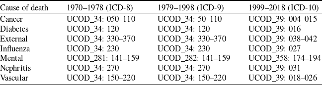


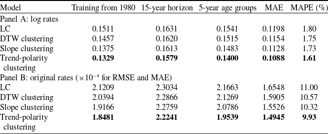
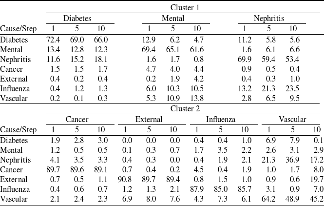
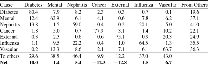


 Open access