


1. Introduction
Understanding the drivers of biodiversity across spatial scales remains a central challenge in ecology and evolutionary biology (see e.g., Benson et al. Reference Benson, Butler, Close, Saupe and Rabosky2021; Mannion et al. Reference Mannion, Upchurch, Benson and Goswami2014). While many empirical studies have established that extant species distributions are influenced by both abiotic (e.g., temperature, elevation and precipitation) and biotic factors, the underlying mechanics of these relationships remain difficult to disentangle (see e.g., Antonelli et al. Reference Antonelli, Kissling, Flantua, Bermúdez, Mulch, Muellner-Riehl, Kreft, Linder, Badgley, Fjeldså, Fritz, Rahbek, Herman, Hooghiemstra and Hoorn2018; Mitchell et al. Reference Mitchell, Qiu, Cardinale, Chan, Eigenbrod, Felipe-Lucia, Jacob, Jones and Sonter2024). These difficulties arise because biodiversity patterns are the result of a single ‘experiment’, comprising a complex history of variation in many environmental variables, as well as a particular evolutionary history (e.g., Benson et al. Reference Benson, Butler, Close, Saupe and Rabosky2021; Benton, Reference Benton2009; Willig et al. Reference Willig, Kaufman and Stevens2003).
Correlative approaches comparing extant species range maps to environmental data have shown associations between environmental heterogeneity and species richness (e.g., Stein et al. Reference Stein, Gerstner and Kreft2014; Tuanmu & Jetz, Reference Tuanmu and Jetz2015). These studies often highlight the role of spatial gradients and identify relationships that vary with spatial scale and taxonomic group (Belmaker & Jetz, Reference Belmaker and Jetz2011; O’Malley et al. Reference O’Malley, Roberts, Mannion, Hackel and Wang2023). However, such correlations do not clarify whether the environment causally drives richness patterns, or whether both variables are structured by spatial autocorrelation, range size effects or historical contingency (Cabral et al. Reference Cabral, Valente and Hartig2017). Understanding how correlations arise, how they change as functions of space and scale, and establishing how, or even if, the environment is significant in determining patterns of species richness across the scales of interest (individuals to continents) are problems to be solved. A general challenge is that areas with similar environmental conditions can contain different numbers of species, demonstrating that local environmental conditions alone do not determine species richness (Koenig, Reference Koenig1999).
There are two fundamental and separate challenges in inferring causality from empirical biodiversity data. The first of these is that many variables contribute to biodiversity patterns. They can be complex and interrelated. They are imperfectly understood, and their histories are at best partially known. Empirical studies have limited control over these variables and hence struggle to isolate their individual effects. The second problem arises from the stochastic nature of evolutionary processes (e.g., genome mutation/drift, organism dispersion; Willig et al. Reference Willig, Kaufman and Stevens2003). Even if the ‘experiment of life’ could be run repeatedly from the same starting point and using the same environmental variables, the stochasticity of evolution would likely result in different eco-evolutionary histories and hence different biodiversity patterns. Empirical studies can make use of only one ‘run’ of the experiment. Thus, they provide limited insight into statistical properties of the system and little information about whether the ‘run’ that generated the observations was typical or anomalous. This lack of information confounds attempts to infer causal relationships between the environment and biodiversity of extant or extinct organisms, as the effects of a particular contingent history cannot be excluded.
To address both of these problems and for consistency, we explore the use of organism-level simulations to investigate how dispersal ability and environmental gradients interact to shape biodiversity patterns. We build on a body of work that has developed the means to predict biodiversity in space and time from evolutionary ‘first principles’. For instance, Gotelli et al. (Reference Gotelli, Anderson, Arita, Chao, Colwell, Connolly, Currie, Dunn, Graves, Green, Grytnes, Jiang, Jetz, Kathleen Lyons, McCain, Magurran, Rahbek, Rangel, Soberón and Willig2009) and Rangel et al. (Reference Rangel, Edwards, Holden, Diniz-Filho, Gosling, Coelho, Cassemiro, Rahbek and Colwell2018) provide methodological frameworks using simulations to understand theoretical and observed macroecological patterns, including biodiversity in the South American continent. The potential of mechanistic approaches to predict biodiversity has been emphasized by Connolly et al. (Reference Connolly, Keith, Colwell and Rahbek2017), Pontarp et al. (Reference Pontarp, Bunnefeld, Cabral, Etienne, Fritz, Gillespie, Graham, Hagen, Hartig, Huang, Jansson, Maliet, Münkemüller, Pellissier, Rangel, Storch, Wiegand and Hurlbert2019) and Dolson & Ofria (Reference Dolson and Ofria2021). Catella & Abbott (Reference Catella and Abbott2023) explored how abiotic heterogeneity influences species densities and spatial biodiversity patterns in digital simulations. Bridle et al. (Reference Bridle, Polechová, Kawata and Butlin2010) showed that dispersal, gradient steepness and carrying capacity can be key determinants of adaptation.
In contrast to modelling approaches that operate at the species level or higher (cf. Gotelli et al. Reference Gotelli, Anderson, Arita, Chao, Colwell, Connolly, Currie, Dunn, Graves, Green, Grytnes, Jiang, Jetz, Kathleen Lyons, McCain, Magurran, Rahbek, Rangel, Soberón and Willig2009; Rangel et al. Reference Rangel, Edwards, Holden, Diniz-Filho, Gosling, Coelho, Cassemiro, Rahbek and Colwell2018; Ruffley et al. Reference Ruffley, Peterson, Week, Tank and Harmon2019; van der Plas et al. Reference van der Plas, Janzen, Ordonez, Fokkema, Reinders, Etienne and Olff2015), organism-level simulation does not require assumptions about patterns and processes at a higher organizational level (Pontarp & Wiens, Reference Pontarp and Wiens2017). Instead, such patterns arise from the behaviour of individuals, as they do in nature (e.g., Dolson & Ofria, Reference Dolson and Ofria2021). While many previous simulation studies rely on only one or a few replicates, we explore whether well-defined statistical distributions emerge when a very large number of experiments containing stochastic evolutionary processes are conducted. By running many ‘experiments of life’ as computational simulations, we are able to isolate and control environmental variables and to develop statistical expectations for biodiversity over a large number of different evolutionary histories. This approach permits assessment of the ‘strength’ of the relationship between richness and environmental gradients and how it is influenced by evolutionary stochasticity.
Specifically, our study tests whether the spatial rate of environmental change emerges as a useful metric to predict biodiversity and under what conditions this relationship holds. To simplify our study, we use a single (abstract) environmental variable, varying spatially in a sinusoidal manner. We quantified the spatial rate of change as the absolute value of the first derivative of this variable; for brevity, we term this metric the spatial derivative. The abstract environmental variable might be conceived of as altitude, for example, in which case the spatial derivative would represent the topographic slope. We test whether linkages between the spatial derivative and biodiversity emerge consistently across replicated simulations when dispersal is sufficient to allow organisms to track environmental variation without homogenizing diversity (Figure 1).
Simplified postulated relationships between environment and species richness tested in this study. (a) Species richness (green) has a simple and direct relationship with environment (black). More formally, species richness is in-phase with the environment. (b) Species richness (green) has simple and direct relationship to environmental rate of change (strictly, the absolute value of the spatial derivative; grey). Strictly, we consider the absolute value of the derivative of the environmental variable (cf. black and grey curves).

We employ the rapid evolutionary simulator (REvoSim; Garwood et al. Reference Garwood, Spencer and Sutton2019), an individual-level simulation model where phenomena such as speciation and adaptation can emerge from evolutionary first principles. REvoSim is computationally efficient – whilst it operates at the level of individual organisms, it can simulate populations of ${10}^{5}-{10}^{7}$
species in spatially structured environments over geological timescales on a typical desktop computer. Simulated organisms evolve through changes within a fixed-length genome (first-order evolution, sensu DeJong & Degens, Reference DeJong and Degens2024). This model has been used by others to test ideas about the relationship between environmental instability, disturbance and biodiversity (Furness et al. Reference Furness, Garwood, Mannion and Sutton2021a; Furness & Sutton, Reference Furness and Sutton2024). By omitting complex interactions like predation or mutualism, REvoSim provides a controlled environment to test whether such complexities are essential for producing the observed macroecological patterns. It has been used to understand how productivity, niche availability and other factors influence species richness and extinction risk in ecosystems (Furness et al. Reference Furness, Garwood, Mannion and Sutton2021b). It can replicate observed phenomena, e.g. species richness patterns and genetic diversity that mimic observations from the real world whilst honouring the fundamental principles of evolution, making it well suited for our goals (see e.g. Garwood et al. Reference Garwood, Spencer and Sutton2019).
${10}^{5}-{10}^{7}$
species in spatially structured environments over geological timescales on a typical desktop computer. Simulated organisms evolve through changes within a fixed-length genome (first-order evolution, sensu DeJong & Degens, Reference DeJong and Degens2024). This model has been used by others to test ideas about the relationship between environmental instability, disturbance and biodiversity (Furness et al. Reference Furness, Garwood, Mannion and Sutton2021a; Furness & Sutton, Reference Furness and Sutton2024). By omitting complex interactions like predation or mutualism, REvoSim provides a controlled environment to test whether such complexities are essential for producing the observed macroecological patterns. It has been used to understand how productivity, niche availability and other factors influence species richness and extinction risk in ecosystems (Furness et al. Reference Furness, Garwood, Mannion and Sutton2021b). It can replicate observed phenomena, e.g. species richness patterns and genetic diversity that mimic observations from the real world whilst honouring the fundamental principles of evolution, making it well suited for our goals (see e.g. Garwood et al. Reference Garwood, Spencer and Sutton2019).
REvoSim represents each organism with a fixed-length binary genome (64 bits in this study). Each organism is located within a specific ‘cell’ in a two-dimensional, spatially structured environment. The first 32 bits of the genome are used to assess the fitness of the organism to the environment; all 64 bits are used to assess reproductive fitness and to identify species. Reproduction is determined by the similarity of the genomes of individuals and the values of environmental variables in the cell. The reader is referred to (Garwood et al. Reference Garwood, Spencer and Sutton2019) for full details of the REvoSim model and software implementation. For convenience, a summary of the methodology relevant to this study is given as in the Supporting Information.
We note that many metrics and proxies for biodiversity are available (see e.g., DeLong, Reference DeLong1996). For instance, the diversity of genes within a group of organisms (genetic diversity) and the count of unique species occupying a specific area (species richness) are both used to assess the variety of life. Although species richness has been criticized as a metric for assessing biodiversity because it does not account for relative abundance, genetic variation or functional traits (see e.g., Gotelli et al. Reference Gotelli, Anderson, Arita, Chao, Colwell, Connolly, Currie, Dunn, Graves, Green, Grytnes, Jiang, Jetz, Kathleen Lyons, McCain, Magurran, Rahbek, Rangel, Soberón and Willig2009; Hillebrand et al. Reference Hillebrand, Blasius, Borer, Chase, Downing, Eriksson, Filstrup, Harpole, Hodapp, Larsen, Lewandowska, Seabloom, Van de Waal and Ryabov2018), it remains widely used, partly because it is relatively easy to determine from real-world data and can also be estimated in a palaeontological context (see e.g., Benson et al. Reference Benson, Butler, Close, Saupe and Rabosky2021 and references therein). In this study, we use species richness, which we assess by counting the number of species within a cell. Given that genetic information is available for every individual in a simulation, we also explore the extent to which species richness correlates with genetic diversity.
Comparisons with data from current-day biota reduce uncertainties that would be associated with interpreting the relatively sparsely sampled history of biodiversity preserved by the fossil record (see e.g., Alroy, Reference Alroy2008; Alroy et al. Reference Alroy, Marshall, Bambach, Bezusko, Foote, Fürsich, Hansen, Holland, Ivany, Jablonski, Jacobs, Jones, Kosnik, Lidgard, Low, Miller, Novack-Gottshall, Olszewski, Patzkowsky and Webber2001). To provide an example of how predictions from REvoSim can be tested against real-world data, we thus analyze extant avian species richness along an equatorial African transect. This region appears to have been broadly geologically and climatically stable, occupying similar latitudes, during the last few million years, increasing compatibility with assumptions in our simulations (e.g., Dagallier et al. Reference Dagallier, Janssens, Dauby, Blach-Overgaard, Mackinder, Droissart, Svenning, Sosef, Stévart, Harris, Sonké, Wieringa, Hardy and Couvreur2020; Jetz et al. Reference Jetz, Rahbek and Colwell2004; Burke, 1996). We test whether species richness along this transect correlates more strongly with the spatial derivative, e.g. the slope of elevation, precipitation or temperature, than with the values of modern environmental variables, acknowledging that these parameter values can change in time (e.g., deMenocal, Reference deMenocal2004). This analysis is provided as a demonstration of how findings from a synthetic model can be linked to detailed empirical biodiversity data. We speculate on how it might be useful for interpreting the fossil record.
In summary, we use replicated, mechanistic simulations to clarify when and how the spatial structure of environments can be straightforwardly related to biodiversity. We establish when ‘noise’ introduced by evolutionary stochasticity conceals the relationship. By isolating the roles of dispersal, environmental variables, and stochastic evolutionary processes, we provide a framework for interpreting large-scale biodiversity patterns beyond classic correlative approaches. Our findings help define the limits of predictability imposed by stochastic evolutionary processes and demonstrate how synthetic models can be used to contextualize the partial information about ancient biodiversity preserved in the fossil record.
2. Methods
2.a. Modelling strategy
In REvoSim, the organisms can reproduce and mutate. Each individual is defined by a 64-bit binary genome, a sequence of zeros and ones (genes). Genomes within populations evolve through stochastic mutation. Genes are also subject to adaptation through selection for fitness in the environment. Organisms reproduce sexually with other organisms in the same cell. Species are automatically identified by REvoSim using the Biological Species Concept, i.e. as reproductively-isolated population groups (Garwood et al. Reference Garwood, Spencer and Sutton2019). When the genetic difference between two organisms exceeds a configurable threshold, they are not able to breed and are classified as distinct species.
We explore simple models in which the environment, $e$
, is determined by integer values,
$e$
, is determined by integer values, $0\le e\le 255$
, in a uniform grid of
$0\le e\le 255$
, in a uniform grid of $X\times Y$
cells or pixels (px), where
$X\times Y$
cells or pixels (px), where $X=Y=100$
. REvoSim maps environmental parameter values to colors in a raster image for visualization purposes. We use an environmental map that varies sinusoidally in the
$X=Y=100$
. REvoSim maps environmental parameter values to colors in a raster image for visualization purposes. We use an environmental map that varies sinusoidally in the $x$
direction and is constant in the
$x$
direction and is constant in the $y$
direction. This setup is analogous to real-world scenarios where organisms must adapt to a single environmental variable that changes along a single spatial dimension. We set the spatial grid to be toroidal, i.e. to ‘wrap around’ in both
$y$
direction. This setup is analogous to real-world scenarios where organisms must adapt to a single environmental variable that changes along a single spatial dimension. We set the spatial grid to be toroidal, i.e. to ‘wrap around’ in both $x$
and
$x$
and $y$
directions, to avoid edge-effects (Porensky & Young, Reference Porensky and Young2013). The sinusoidal wavelength chosen (
$y$
directions, to avoid edge-effects (Porensky & Young, Reference Porensky and Young2013). The sinusoidal wavelength chosen ( $\lambda $
= 50 px) provides this ‘wrap around’ in the
$\lambda $
= 50 px) provides this ‘wrap around’ in the $x$
direction without discontinuities (Figure 2f).
$x$
direction without discontinuities (Figure 2f).
An example of species dispersion in a single simulation and dispersion parameters included in this study. (a-e) Biodiversity in a single simulation after 100, 200, 1000, 10,000 and 100,000 steps. This simulation has spatial dimensions of 100 $\times $
100 pixels (white vectors in panel a; see body text for extended description). Colors correspond to the most abundant species in a pixel at any given time; colors for species are chosen arbitrarily. Black indicates no organisms present. (a-b) The first organism (green), inserted into the centre of the domain, reproduces and disperses to other pixels. (c) Colonization of the whole domain. (d-e) Different colors show that speciation has occurred and new species are now most abundant in certain pixels. (f) Map showing the simple sinusoidal environment and dispersion parameters, d, used to control dispersion of offspring in this study. White violin plots show probabilities of dispersion for each dispersion parameter at the scale of the environment; black dots = mean dispersion,
$\times $
100 pixels (white vectors in panel a; see body text for extended description). Colors correspond to the most abundant species in a pixel at any given time; colors for species are chosen arbitrarily. Black indicates no organisms present. (a-b) The first organism (green), inserted into the centre of the domain, reproduces and disperses to other pixels. (c) Colonization of the whole domain. (d-e) Different colors show that speciation has occurred and new species are now most abundant in certain pixels. (f) Map showing the simple sinusoidal environment and dispersion parameters, d, used to control dispersion of offspring in this study. White violin plots show probabilities of dispersion for each dispersion parameter at the scale of the environment; black dots = mean dispersion, $\mu $
.
$\mu $
. $d=15$
for simulation shown in panels (a–e). See body text for details.
$d=15$
for simulation shown in panels (a–e). See body text for details.

In a series of systematic experiments, we varied the capability of organisms to disperse. REvoSim default settings were otherwise used for all other parameters. At the start of each experiment, a population of genetically identical organisms was inserted into the cell at the centre of the environment, where they started reproduction, mutation and dispersal. The experiments were then iterated for $T=100,000$
steps, which could represent
$T=100,000$
steps, which could represent $O(0.1-1$
Myr) of vertebrate evolution. Species richness broadly increased in each experiment until
$O(0.1-1$
Myr) of vertebrate evolution. Species richness broadly increased in each experiment until $\sim\!\!50,000$
steps, after which it typically stabilized (Figures 2a–e & 3). Replicate experiments (
$\sim\!\!50,000$
steps, after which it typically stabilized (Figures 2a–e & 3). Replicate experiments ( $N=3000$
) were produced for each scenario (i.e. for each dispersal setting). This Monte Carlo experimentation allows statistical understanding of expected species richness from models incorporating evolutionary stochasticity, which can experience very different trajectories across replicates (Figure 3).
$N=3000$
) were produced for each scenario (i.e. for each dispersal setting). This Monte Carlo experimentation allows statistical understanding of expected species richness from models incorporating evolutionary stochasticity, which can experience very different trajectories across replicates (Figure 3).
Variability of species richness in time from Monte Carlo experimentation. (a) Grey curves = species richness as a function of time in $N=3000$
simulations. Environmental variable (
$N=3000$
simulations. Environmental variable ( $\lambda =50$
px) and dispersion parameter (
$\lambda =50$
px) and dispersion parameter ( $d=15$
; see Figure 1f) were held constant. Gene mutation, reproduction and dispersion are stochastic (see body text for extended description). Green line = trajectory of simulation depicted in Figure 1a–e. Black line = mean species richness,
$d=15$
; see Figure 1f) were held constant. Gene mutation, reproduction and dispersion are stochastic (see body text for extended description). Green line = trajectory of simulation depicted in Figure 1a–e. Black line = mean species richness, $\bar {S}$
, from the 3000 simulations. (b) Grey histogram and black line = distribution of species richness and
$\bar {S}$
, from the 3000 simulations. (b) Grey histogram and black line = distribution of species richness and $\bar {S}$
at
$\bar {S}$
at $T=\mathrm{100,000}$
, respectively.
$T=\mathrm{100,000}$
, respectively.

2.b. Evolutionary stochasticity
REvoSim experiments included four sources of stochasticity. Two represent per-replicate determination of initial conditions, specifically generation of a ‘fitness landscape’ (McCandlish, Reference McCandlish2011; McGhee, Reference McGhee2006), and selection of a viable genome for the initial population (see Garwood et al. Reference Garwood, Spencer and Sutton2019). Stochasticity during each replicate occurred in mutation (see Garwood et al. Reference Garwood, Spencer and Sutton2019) and in dispersal; the latter is discussed here in more detail.
REvoSim organisms do not move, but offspring of reproductive events ‘disperse’, i.e. attempt to establish themselves either in the same pixel as their parents, or in a nearby pixel. The dispersal distance is defined as
 $$D = \left| {{C \over d}} \right|,$$
where the dispersal parameter, $d$
, is set at the beginning of each experiment and is constant for all organisms. The parameter
$d$
, is set at the beginning of each experiment and is constant for all organisms. The parameter $C=\sqrt{65536/(b+1)}-16$
controls the stochasticity of dispersal via the value of
$C=\sqrt{65536/(b+1)}-16$
controls the stochasticity of dispersal via the value of $b$
, which is chosen randomly from a uniform distribution
$b$
, which is chosen randomly from a uniform distribution $0\le b\le 255$
(thus
$0\le b\le 255$
(thus $0\le C\le 240$
). In practice, displacement is determined by defining translation along the
$0\le C\le 240$
). In practice, displacement is determined by defining translation along the $x$
and
$x$
and $y$
axes
$y$
axes
 $${D_x} = {C \over d}{\rm{sin}}\left( \alpha \right),\,\,{D_y} = {C \over d}{\rm{cos}}\left( \alpha \right){\rm\,\,{thus}}\,\,D = \sqrt {D_x^2 + D_y^2}, $$
with the azimuth of displacement, ${0}^{\circ } \lt \alpha \le {360}^{\circ }$
, chosen randomly from a uniform distribution (Garwood et al. Reference Garwood, Spencer and Sutton2019).
${0}^{\circ } \lt \alpha \le {360}^{\circ }$
, chosen randomly from a uniform distribution (Garwood et al. Reference Garwood, Spencer and Sutton2019).
The dispersal of an organism is inversely proportional to $d$
, with minimum and maximum values of zero px and
$d$
, with minimum and maximum values of zero px and ${D}_{max}=240/d$
px, respectively. The distribution of dispersal distances is weighted towards low values. The values of
${D}_{max}=240/d$
px, respectively. The distribution of dispersal distances is weighted towards low values. The values of $d$
used in this study, along with associated dispersal distributions and mean dispersal,
$d$
used in this study, along with associated dispersal distributions and mean dispersal, $\mu $
(px), are given in Figure 2f. Figure 2a–e shows an example of species spreading across the model domain (via reproduction and dispersal), during
$\mu $
(px), are given in Figure 2f. Figure 2a–e shows an example of species spreading across the model domain (via reproduction and dispersal), during $100,000$
time steps; in this example, the probability that offspring will disperse to within
$100,000$
time steps; in this example, the probability that offspring will disperse to within $D=2$
px of their source pixel (containing their parents) is
$D=2$
px of their source pixel (containing their parents) is $88\mathrm{\%}$
.
$88\mathrm{\%}$
.
As an example, Figure 3a shows species richness trajectories for all replicates for one parametrization of dispersal ( $d=15$
). Mean species richness for all replicates (black curve) and the experiment shown in Figure 2a–e (green curve) is indicated. Figure 3b shows the distribution of species richness for all replicates with
$d=15$
). Mean species richness for all replicates (black curve) and the experiment shown in Figure 2a–e (green curve) is indicated. Figure 3b shows the distribution of species richness for all replicates with $d=15$
.
$d=15$
.
2.c. Metrics of species richness and genetic diversity
Two types of logs were generated for each individual experiment. The first type records species richness every 50 time steps (referred to as ‘species counts’ by REvoSim). These were configured as ‘v2.0.0 CSV’ logs in REvoSim settings, and were used to extract species richness across the grid. The second type records the genomes, species identifications and spatial locations for all individuals present at the final step ( $T=100,000$
). These were used to calculate the mean species richness at each pixel and to calculate genetic diversity across the grid.
$T=100,000$
). These were used to calculate the mean species richness at each pixel and to calculate genetic diversity across the grid.
Species richness for each pixel in each replicate was calculated by counting the unique number of species present in that pixel. These results are used to calculate mean species richness at each $x$
position on the grid (i.e. averaging over all
$x$
position on the grid (i.e. averaging over all $y$
pixels for each
$y$
pixels for each $x$
position), for each value of
$x$
position), for each value of $d$
(see Figure 4f). Species richness for the whole domain was also calculated for each replicate by counting the unique number of species present in the whole
$d$
(see Figure 4f). Species richness for the whole domain was also calculated for each replicate by counting the unique number of species present in the whole $100\times 100$
pixel grid. These values were then compared with the genetic diversity of the corresponding replicate.
$100\times 100$
pixel grid. These values were then compared with the genetic diversity of the corresponding replicate.
Distribution of species richness at steady-state from Monte Carlo experimentation. (a) Environment; blue/black = high/low values; $\lambda =50$
px. (b) Absolute values of the derivative of the environment; white/black = low/high. (c) Mean species richness for each pixel at
$\lambda =50$
px. (b) Absolute values of the derivative of the environment; white/black = low/high. (c) Mean species richness for each pixel at $T=\mathrm{100,000}$
steps from the 3,000 simulations (
$T=\mathrm{100,000}$
steps from the 3,000 simulations ( $d=15$
; see Figure 2f). (d) and (e) transects across the centre of the environment (panel a; at
$d=15$
; see Figure 2f). (d) and (e) transects across the centre of the environment (panel a; at $y=50$
) and the absolute values of its derivative (b), respectively. (f) Transects across mean species richness shown in panel (c); grey curves = transects at
$y=50$
) and the absolute values of its derivative (b), respectively. (f) Transects across mean species richness shown in panel (c); grey curves = transects at $y=1,\dots, 100$
; purple curve = mean species richness for all 100 transects.
$y=1,\dots, 100$
; purple curve = mean species richness for all 100 transects.

We used the following terminology to describe species richness. $S(x,y)$
refers to the species richness of cell
$S(x,y)$
refers to the species richness of cell $(x,y)$
for a particular value of
$(x,y)$
for a particular value of $d$
, in a particular replicate
$d$
, in a particular replicate $n$
. See Figure S1 shows a schematic of the model setup and associated statistics. All of the following statistics were calculated using only the
$n$
. See Figure S1 shows a schematic of the model setup and associated statistics. All of the following statistics were calculated using only the $N$
replicates that had extant species at
$N$
replicates that had extant species at $T=100,000$
. In practice, more than 92% of all simulations are included in these results.
$T=100,000$
. In practice, more than 92% of all simulations are included in these results. $\bar {S}(x,y)$
is the mean species richness of cell
$\bar {S}(x,y)$
is the mean species richness of cell $(x,y)$
for a particular value of
$(x,y)$
for a particular value of $d$
.
$d$
. ${S}_{n}$
is the number of unique species across the entire grid for an individual replicate,
${S}_{n}$
is the number of unique species across the entire grid for an individual replicate, $n$
.
$n$
. $\overline{{S}_{N}}$
is the mean number of species across the entire grid for a particular value of
$\overline{{S}_{N}}$
is the mean number of species across the entire grid for a particular value of $d$
, over all replicates,
$d$
, over all replicates,
![]() .
. $\overline{{S}_{x}}$
is the mean species richness as a function of
$\overline{{S}_{x}}$
is the mean species richness as a function of $x$
, for a particular value of
$x$
, for a particular value of $d$
incorporating all replicates. This value is calculated as the mean of
$d$
incorporating all replicates. This value is calculated as the mean of $\bar {S}(x,y)$
for a given
$\bar {S}(x,y)$
for a given $x$
. For example, at
$x$
. For example, at $x=50$
,
$x=50$
,
![]() .
. ${\overline{{S}_{x}}}_{max}$
is the maximum value of
${\overline{{S}_{x}}}_{max}$
is the maximum value of $\overline{{S}_{x}}$
for a specific value of
$\overline{{S}_{x}}$
for a specific value of $y$
and
$y$
and $d$
. In addition, we calculated the normalized value of mean species richness as a function of
$d$
. In addition, we calculated the normalized value of mean species richness as a function of $x$
, calculated using min–max feature scaling,
$x$
, calculated using min–max feature scaling, $(\overline{{S}_{x}}-{\overline{{S}_{x}}}_{\mathrm{m}\mathrm{i}\mathrm{n}})/$ $({\overline{{S}_{x}}}_{\mathrm{m}\mathrm{a}\mathrm{x}}-{\overline{{S}_{x}}}_{\mathrm{m}\mathrm{i}\mathrm{n}})$
and annotated as
$({\overline{{S}_{x}}}_{\mathrm{m}\mathrm{a}\mathrm{x}}-{\overline{{S}_{x}}}_{\mathrm{m}\mathrm{i}\mathrm{n}})$
and annotated as $\overline{{S}_{x}}/{\overline{{S}_{x}}}_{max}$
for simplicity. This normalized value is used to compare
$\overline{{S}_{x}}/{\overline{{S}_{x}}}_{max}$
for simplicity. This normalized value is used to compare $\overline{{S}_{x}}$
across the different values of
$\overline{{S}_{x}}$
across the different values of $d$
.
$d$
.
Mean genetic diversity in a single replicate, ${\overline{\pi }}_{n}$
, was calculated by comparing genomes from
${\overline{\pi }}_{n}$
, was calculated by comparing genomes from $M$
pairs of individuals,
$M$
pairs of individuals,
 $${\overline \pi _n} = {1 \over M}\sum\limits_{m = 1}^M {\sum\limits_{i = 1}^{64} | } I_1^{i,m} - I_2^{i,m}|,$$
where ${I}_{1}$
and
${I}_{1}$
and ${I}_{2}$
are the individuals whose genomes were compared, and
${I}_{2}$
are the individuals whose genomes were compared, and $i=1,2,\dots, 64$
is the index of genes for each genome for each individual. Since genes are binary digits (either 0 or 1),
$i=1,2,\dots, 64$
is the index of genes for each genome for each individual. Since genes are binary digits (either 0 or 1), ${\overline{\pi }}_{n}=0$
when all individuals are genetically identical. For theoretical scenarios in which all individuals have completely different genomes
${\overline{\pi }}_{n}=0$
when all individuals are genetically identical. For theoretical scenarios in which all individuals have completely different genomes ${\overline{\pi }}_{n}=64$
. It is possible to calculate the true mean genetic diversity for each replicate. However, as the number of individuals present during each replicate (
${\overline{\pi }}_{n}=64$
. It is possible to calculate the true mean genetic diversity for each replicate. However, as the number of individuals present during each replicate ( $I$
) can exceed 100,000, the total number of unique pairs (
$I$
) can exceed 100,000, the total number of unique pairs ( $I(I-1)/2$
) can exceed 10 billion, rendering exhaustive comparison computationally impractical. Instead, we estimated
$I(I-1)/2$
) can exceed 10 billion, rendering exhaustive comparison computationally impractical. Instead, we estimated ${\overline{\pi }}_{n}$
from a sample of the total number of pairings, by comparing
${\overline{\pi }}_{n}$
from a sample of the total number of pairings, by comparing $M=I/2$
randomly chosen unique pairs. Thus, we typically compared
$M=I/2$
randomly chosen unique pairs. Thus, we typically compared $\gt 90,000$
pairs of individuals for each replicate. Figure 5 plots mean genetic diversity for each replicate,
$\gt 90,000$
pairs of individuals for each replicate. Figure 5 plots mean genetic diversity for each replicate, ${\overline{\pi }}_{n}$
compared with its respective species richness,
${\overline{\pi }}_{n}$
compared with its respective species richness, ${S}_{n}$
.
${S}_{n}$
.
Genetic diversity versus species richness at equilibrium. (a) Species richness and genetic diversity compared at $T=\mathrm{100,000}$
for
$T=\mathrm{100,000}$
for $N$
replicates with dispersion parameter
$N$
replicates with dispersion parameter $d=3$
(see Figure 6a). (b–l) Results for different values of dispersion parameter (annotated).
$d=3$
(see Figure 6a). (b–l) Results for different values of dispersion parameter (annotated).

2.d. Real-world data
An equatorial transect of Africa is used to demonstrate how results from simulation can be used to contextualize real-world observations (see Figure S5). Mean annual precipitation, temperature and temperature range from 1981–2010, were extracted from the Climatologies at high resolution for the Earth’s land surface areas (CHELSA) dataset (Karger et al. Reference Karger, Conrad, Böhner, Kawohl, Kreft, Soria-Auza, Zimmermann, Linder and Kessler2017) at a resolution of 30 arcseconds ( $\approx 1$
km at the equator). We note that CHELSA data have been used in previous studies modelling species distributions (e.g., Doninck et al. Reference Doninck, Jones, Zuquim, Ruokolainen, Moulatlet, Sirén, Cárdenas, Lehtonen and Tuomisto2020; Karger et al. Reference Karger, Conrad, Böhner, Kawohl, Kreft, Soria-Auza, Zimmermann, Linder and Kessler2017; Morales-Barbero & Vega-Álvarez, Reference Morales-Barbero and Vega-Álvarez2019). Elevation data were extracted from ETOPO1 (Amante & Eakins, Reference Amante and Eakins2009), with a resolution of 1 arcminute (
$\approx 1$
km at the equator). We note that CHELSA data have been used in previous studies modelling species distributions (e.g., Doninck et al. Reference Doninck, Jones, Zuquim, Ruokolainen, Moulatlet, Sirén, Cárdenas, Lehtonen and Tuomisto2020; Karger et al. Reference Karger, Conrad, Böhner, Kawohl, Kreft, Soria-Auza, Zimmermann, Linder and Kessler2017; Morales-Barbero & Vega-Álvarez, Reference Morales-Barbero and Vega-Álvarez2019). Elevation data were extracted from ETOPO1 (Amante & Eakins, Reference Amante and Eakins2009), with a resolution of 1 arcminute ( $\approx 2$
km at the equator). The derivatives of each variable were calculated using the central differences.
$\approx 2$
km at the equator). The derivatives of each variable were calculated using the central differences.
For species richness, birds were selected as an exemplar group for their well-documented distribution on the continent (Claramunt & Cracraft, Reference Claramunt and Cracraft2015; Fuchs et al. Reference Fuchs, Fjeldså and Pasquet2006; and Oliveros et al. Reference Oliveros, Field, Ksepka, Barker, Aleixo, Andersen, Alström, Benz, Braun, Braun, Bravo, Brumfield, Chesser, Claramunt, Cracraft, Cuervo, Derryberry, Glenn, Harvey and Faircloth2019) and the availability of data. Avian species richness was extracted from Jenkins et al. (Reference Jenkins, Pimm and Joppa2013) expert range map, which has a resolution of $10\times 10$
km.
$10\times 10$
km.
All transects were sampled from each dataset at $10$
km intervals.
$10$
km intervals.
Species richness estimates from range maps may be unreliable at fine scales (Cohen & Jetz, Reference Cohen and Jetz2024; Graham & Hijmans, Reference Graham and Hijmans2006; Hurlbert & Jetz, Reference Hurlbert and Jetz2007). Hurlbert & Jetz, (Reference Hurlbert and Jetz2007) demonstrate that atlas data and range maps of bird species in Africa correlate well at resolutions $\gt {2}^{\circ }$
(
$\gt {2}^{\circ }$
( $\approx 200$
km), which suggests that focusing our analysis on larger scales might be prudent. We therefore removed wavelengths (scales)
$\approx 200$
km), which suggests that focusing our analysis on larger scales might be prudent. We therefore removed wavelengths (scales) $\,\lesssim\, 200$
km using a Gaussian filter before comparing the spatial series. For comparison, we also generate results for wavelengths
$\,\lesssim\, 200$
km using a Gaussian filter before comparing the spatial series. For comparison, we also generate results for wavelengths $\gtrsim $
1000 km. Pearson’s product-moment correlation coefficients and p-values were calculated between avian species richness and (a) environmental variables, and (b) the absolute values of the spatial derivatives of the environmental variables.
$\gtrsim $
1000 km. Pearson’s product-moment correlation coefficients and p-values were calculated between avian species richness and (a) environmental variables, and (b) the absolute values of the spatial derivatives of the environmental variables.
3. Results
3.a. Mean species richness varies with dispersal ability
Figure 5 shows genetic diversity compared to species richness in simulations at ‘equilibrium’ (at $T=100,000$
). Diversity and richness covary positively,
$T=100,000$
). Diversity and richness covary positively, $\mathrm{C}\mathrm{o}\mathrm{v}(\overline{{S}_{n}},\overline{{\pi }_{n}}) \gt 0$
, in simulations that incorporate relatively high dispersal abilities, i.e.
$\mathrm{C}\mathrm{o}\mathrm{v}(\overline{{S}_{n}},\overline{{\pi }_{n}}) \gt 0$
, in simulations that incorporate relatively high dispersal abilities, i.e. $d \lt 40$
:
$d \lt 40$
: ${D}_{max}\ge 6$
px,
${D}_{max}\ge 6$
px, $\mu \ge 0.4$
px. When dispersal ability is relatively low (
$\mu \ge 0.4$
px. When dispersal ability is relatively low ( $d\ge 40$
, Figure 5k–l), covariance is close to zero,
$d\ge 40$
, Figure 5k–l), covariance is close to zero, $\mathrm{C}\mathrm{o}\mathrm{v}(\overline{{S}_{n}},\overline{{\pi }_{n}})\approx 0$
. However, this arises because the variance in both metrics is very low, resulting in the covariance being ‘swamped’ by stochastic noise. These results indicate that, in this system, species richness is a good proxy for genetic diversity. Species richness is the simpler quantity to measure or estimate in empirical data (for both extant and extinct biota; see, e.g., Benson et al. Reference Benson, Butler, Close, Saupe and Rabosky2021; Jetz et al. Reference Jetz, McPherson and Guralnick2012); consequently, we use only species richness in our analyses.
$\mathrm{C}\mathrm{o}\mathrm{v}(\overline{{S}_{n}},\overline{{\pi }_{n}})\approx 0$
. However, this arises because the variance in both metrics is very low, resulting in the covariance being ‘swamped’ by stochastic noise. These results indicate that, in this system, species richness is a good proxy for genetic diversity. Species richness is the simpler quantity to measure or estimate in empirical data (for both extant and extinct biota; see, e.g., Benson et al. Reference Benson, Butler, Close, Saupe and Rabosky2021; Jetz et al. Reference Jetz, McPherson and Guralnick2012); consequently, we use only species richness in our analyses.
Species richness for the entire domain varied between 1 (only one species present) and 10,000 (all pixels occupied by a different species) over the full range of experiments. The highest mean species richness, $\overline{{S}_{N}}$
, at the final step of the model occurred at
$\overline{{S}_{N}}$
, at the final step of the model occurred at $d=50$
(
$d=50$
( ${D}_{max}=4.8$
px,
${D}_{max}=4.8$
px, $\mu =0.3$
px; see Figure S3). Figures 3b and S4 show that frequency distributions of species richness tend to be skewed towards low values for high dispersal (
$\mu =0.3$
px; see Figure S3). Figures 3b and S4 show that frequency distributions of species richness tend to be skewed towards low values for high dispersal ( $d\le 20$
,
$d\le 20$
, ${D}_{max}\ge 12$
px,
${D}_{max}\ge 12$
px, $\mu \ge 0.7$
px), and to be Gaussian or slightly skewed towards higher values for low dispersal (
$\mu \ge 0.7$
px), and to be Gaussian or slightly skewed towards higher values for low dispersal ( $d\ge 25$
,
$d\ge 25$
, ${D}_{max}\le 10$
px,
${D}_{max}\le 10$
px, $\mu \le 0.6$
px).
$\mu \le 0.6$
px).
3.b. Relationship between diversity and environment in simulations
Figure 4 illustrates the spatial distribution of the environmental parameter, $e$
, the absolute value of its derivative
$e$
, the absolute value of its derivative $\left|\dot{e}\right|=|\mathrm{d}e/\mathrm{d}x|$
(for brevity referred to as the spatial derivative), and mean species richness,
$\left|\dot{e}\right|=|\mathrm{d}e/\mathrm{d}x|$
(for brevity referred to as the spatial derivative), and mean species richness, $\overline{{S}_{x}}$
, for a representative value of
$\overline{{S}_{x}}$
, for a representative value of $d=15$
. Visual inspection of these results shows that species richness is highly correlated with the absolute derivative of the environmental parameter,
$d=15$
. Visual inspection of these results shows that species richness is highly correlated with the absolute derivative of the environmental parameter, $\left|\dot{e}\right|$
, rather than with
$\left|\dot{e}\right|$
, rather than with $e$
itself. Normalized results for other values of
$e$
itself. Normalized results for other values of $d$
are shown in Figure 6. For clarity,
$d$
are shown in Figure 6. For clarity, $\left|\dot{e}\right|$
was normalized by its maximum value such that
$\left|\dot{e}\right|$
was normalized by its maximum value such that $0\le \left|\dot{e}\right|/|\dot{e}{|}_{max}\le 1$
. The highest value of value of
$0\le \left|\dot{e}\right|/|\dot{e}{|}_{max}\le 1$
. The highest value of value of $\overline{S}(x,y)$
was
$\overline{S}(x,y)$
was $2.78$
, recorded for
$2.78$
, recorded for $d=35$
(
$d=35$
( ${D}_{max}=8$
px,
${D}_{max}=8$
px, $\mu =0.5$
px).
$\mu =0.5$
px).
Relationships between environment and species richness as a function of dispersion. (a–l) All simulations used the same environment (see Figure 4; $\lambda =50$
px). Dispersion ability was varied by systematically changing the value of dispersion parameter,
$\lambda =50$
px). Dispersion ability was varied by systematically changing the value of dispersion parameter, $d$
, see panel annotations and Figure 2f (note low
$d$
, see panel annotations and Figure 2f (note low $d$
indicates higher dispersion). Grey curves = absolute value of the derivative of the environmental variable,
$d$
indicates higher dispersion). Grey curves = absolute value of the derivative of the environmental variable, $\left|\underline{e}\right|$
, normalized using min-max feature scaling,
$\left|\underline{e}\right|$
, normalized using min-max feature scaling, $\left(\right|\underline{e}|-|\underline{e}{|}_{min})/(|\underline{e}{|}_{max}-|\underline{e}{|}_{min})$
, as a function of
$\left(\right|\underline{e}|-|\underline{e}{|}_{min})/(|\underline{e}{|}_{max}-|\underline{e}{|}_{min})$
, as a function of $x$
coordinate (see Figure 4e). Dark green curves = transects of mean species richness,
$x$
coordinate (see Figure 4e). Dark green curves = transects of mean species richness, $\overline{{S}_{x}}$
, (along the
$\overline{{S}_{x}}$
, (along the $x$
coordinate; see Figure 4f) for 3,000 simulations with given value of
$x$
coordinate; see Figure 4f) for 3,000 simulations with given value of $d$
, normalized by using min-max feature scaling
$d$
, normalized by using min-max feature scaling $(\overline{{S}_{x}}-{\overline{{S}_{x}}}_{min})/({\overline{{S}_{x}}}_{max}-{\overline{{S}_{x}}}_{min})$
. Light green curves = mean species richness transects at
$(\overline{{S}_{x}}-{\overline{{S}_{x}}}_{min})/({\overline{{S}_{x}}}_{max}-{\overline{{S}_{x}}}_{min})$
. Light green curves = mean species richness transects at $y=1, \ldots, 100$
, calculated from all
$y=1, \ldots, 100$
, calculated from all $\approx \mathrm{3,000}$
experiments, each line normalized using min-max feature scaling.
$\approx \mathrm{3,000}$
experiments, each line normalized using min-max feature scaling.

Pearson’s correlation coefficients, $r$
, between
$r$
, between $\overline{{S}_{x}}$
and
$\overline{{S}_{x}}$
and $\left|\dot{e}\right|$
are shown for each value of
$\left|\dot{e}\right|$
are shown for each value of $d$
tested in Figure 7. High correlations (
$d$
tested in Figure 7. High correlations ( $r \gt 0.8$
) were observed for
$r \gt 0.8$
) were observed for $d \lt 35$
(
$d \lt 35$
( ${D}_{max} \gt 7$
px,
${D}_{max} \gt 7$
px, $\mu \gt 0.4$
px; cf. Figure 6).
$\mu \gt 0.4$
px; cf. Figure 6).
Correlation between mean species richness, derivative of the environment, and environment as a function of dispersion. (a-c) Correlation between normalized mean species richness, $\overline{{S}_{x}}/{\overline{{S}_{x}}}_{max}$
, and normalized environmental derivative,
$\overline{{S}_{x}}/{\overline{{S}_{x}}}_{max}$
, and normalized environmental derivative, $\left|\underline{e}\right|/|\underline{e}{|}_{max}$
, for
$\left|\underline{e}\right|/|\underline{e}{|}_{max}$
, for $d=\mathrm{50,30,8}$
. See respective dark green and grey curves in Figure 6. Coloured lines = linear regression, with the correlation coefficient,
$d=\mathrm{50,30,8}$
. See respective dark green and grey curves in Figure 6. Coloured lines = linear regression, with the correlation coefficient, $r$
, annotated above each plot. (d) Summary of correlation,
$r$
, annotated above each plot. (d) Summary of correlation, $r$
, between normalized mean species richness and environmental derivative (grey dots) and environment (black dots) for annotated maximum dispersion,
$r$
, between normalized mean species richness and environmental derivative (grey dots) and environment (black dots) for annotated maximum dispersion, ${D}_{max}$
, and dispersion parameter,
${D}_{max}$
, and dispersion parameter, $d$
, values. Error bars = range of coefficients calculated for all,
$d$
, values. Error bars = range of coefficients calculated for all, $y=1,\ldots, 100$
, transects in each systematic test of
$y=1,\ldots, 100$
, transects in each systematic test of $d$
shown in Figure 6. Coloured dots correspond to panels (a-c).
$d$
shown in Figure 6. Coloured dots correspond to panels (a-c).

3.c. Relationship between diversity and environment in a real-world transect
Figure 8 shows avian species richness, mean annual precipitation ( $Pn$
), elevation (
$Pn$
), elevation ( $E$
), temperature (
$E$
), temperature ( $T$
), temperature range (
$T$
), temperature range ( $\mathrm{\Delta }T$
) and their absolute derivatives along the African equatorial transect. The respective Pearson’s correlation coefficients,
$\mathrm{\Delta }T$
) and their absolute derivatives along the African equatorial transect. The respective Pearson’s correlation coefficients, $r$
, are annotated for each panel and significance (
$r$
, are annotated for each panel and significance ( $p \lt 0.05$
) is indicated by asterisks. Species richness is positively (
$p \lt 0.05$
) is indicated by asterisks. Species richness is positively ( $0.61\le r\le 0.82$
) and significantly correlated with the absolute derivatives of all four environmental variables for wavelengths
$0.61\le r\le 0.82$
) and significantly correlated with the absolute derivatives of all four environmental variables for wavelengths $\gtrsim\, 200$
km (Figure 8e–h). We note that correlations between species richness and the absolute derivatives of environmental variables are even higher (
$\gtrsim\, 200$
km (Figure 8e–h). We note that correlations between species richness and the absolute derivatives of environmental variables are even higher ( $0.75\le r\le 0.92$
) at wavelengths
$0.75\le r\le 0.92$
) at wavelengths $\gtrsim 1000$
km (see Figure S6). In contrast, the only environmental variable examined with significant correlation with species richness is elevation (
$\gtrsim 1000$
km (see Figure S6). In contrast, the only environmental variable examined with significant correlation with species richness is elevation ( $r=0.86$
; otherwise
$r=0.86$
; otherwise $r \lt 0.1$
; Figure 8a–d).
$r \lt 0.1$
; Figure 8a–d).
Correlations between Equatorial avian species richness in Africa and precipitation, elevation, temperature, its range and their absolute derivatives. Green curves = avian species richness extracted from Jenkins et al. (Reference Jenkins, Pimm and Joppa2013) $10\times 10$
km grid, Gaussian filtered to remove wavelengths
$10\times 10$
km grid, Gaussian filtered to remove wavelengths $\lesssim\, 200$
km. (a-d) Mean annual precipitation (
$\lesssim\, 200$
km. (a-d) Mean annual precipitation ( $Pn$
, m), elevation (
$Pn$
, m), elevation ( $E$
, km), temperature (
$E$
, km), temperature ( $T$
,
$T$
, ${}^{\circ }$
C) and temperature range (
${}^{\circ }$
C) and temperature range ( $\Delta T$
,
$\Delta T$
, ${}^{\circ }$
C), respectively, from 1981 to 2010 (Amante & Eakins, Reference Amante and Eakins2009; Karger et al. Reference Karger, Conrad, Böhner, Kawohl, Kreft, Soria-Auza, Zimmermann, Linder and Kessler2017). All transects were Gaussian filtered to remove wavelengths
${}^{\circ }$
C), respectively, from 1981 to 2010 (Amante & Eakins, Reference Amante and Eakins2009; Karger et al. Reference Karger, Conrad, Böhner, Kawohl, Kreft, Soria-Auza, Zimmermann, Linder and Kessler2017). All transects were Gaussian filtered to remove wavelengths $\lesssim 200$
km. (e-h) Absolute values of the derivatives of mean annual precipitation (mm/km), topography (m/km), temperature (
$\lesssim 200$
km. (e-h) Absolute values of the derivatives of mean annual precipitation (mm/km), topography (m/km), temperature ( ${}^{\circ }$
C/km) and temperature range (
${}^{\circ }$
C/km) and temperature range ( ${}^{\circ }$
C/km). Pearson’s correlation coefficient (
${}^{\circ }$
C/km). Pearson’s correlation coefficient ( $r$
) for species richness and each environmental variable or its absolute derivative are annotated in their respective panels (a-h); asterisks indicate significant p-values (
$r$
) for species richness and each environmental variable or its absolute derivative are annotated in their respective panels (a-h); asterisks indicate significant p-values ( $p \lt 0.05$
). See Figures S5 and S6 for full resolution series and filtering to remove wavelengths
$p \lt 0.05$
). See Figures S5 and S6 for full resolution series and filtering to remove wavelengths $\lesssim 1000$
km.
$\lesssim 1000$
km.

4. Discussion
4.a. Spatial rate of change, species richness and the role of dispersal
Species richness in the simulated ecosystems, and in our exemplar real-world dataset, correlates positively with the spatial derivative, $\left|\dot{e}\right|$
. In other words, these results reinforce the idea that the intensity of spatial variation of an environment appears to be a useful predictor of the number of species within a given area, even when evolutionary processes are permitted to modify biodiversity (cf. Benson et al. Reference Benson, Butler, Close, Saupe and Rabosky2021; Stein et al. Reference Stein, Gerstner and Kreft2014; Tuanmu & Jetz, Reference Tuanmu and Jetz2015). There are two important caveats: first, the dispersal distances of the organisms involved must be sufficiently high. Secondly, a single ‘experiment of life’ (model realization) may not provide sufficient information to identify this relationship, even if it should be expected (in the statistical sense). It emerges by generating statistical insights, i.e. by running many experiments.
$\left|\dot{e}\right|$
. In other words, these results reinforce the idea that the intensity of spatial variation of an environment appears to be a useful predictor of the number of species within a given area, even when evolutionary processes are permitted to modify biodiversity (cf. Benson et al. Reference Benson, Butler, Close, Saupe and Rabosky2021; Stein et al. Reference Stein, Gerstner and Kreft2014; Tuanmu & Jetz, Reference Tuanmu and Jetz2015). There are two important caveats: first, the dispersal distances of the organisms involved must be sufficiently high. Secondly, a single ‘experiment of life’ (model realization) may not provide sufficient information to identify this relationship, even if it should be expected (in the statistical sense). It emerges by generating statistical insights, i.e. by running many experiments.
Consider Figure 9, in which the regions (both with spatial range $\mathrm{\Delta }x$
) labelled i and ii represents areas with low and high environmental variability (
$\mathrm{\Delta }x$
) labelled i and ii represents areas with low and high environmental variability ( $\mathrm{\Delta }e$
), respectively. In other words, the environmental conditions in cells are more similar to their near neighbours in region i than in region ii. As a consequence, offspring of parents living in cells in region i are more likely to be adapted to nearby cells, and thus be able to successfully settle in them. Consequently, gene flow, which requires successful settling in non-parental cells, is greater in region i than in ii. Gene flow between cells tends to homogenize the genomes of populations; adaptation to their local environments tends to differentiate them, eventually into different species (Coyne et al. Reference Coyne, Orr, Coyne and Orr2004). The balance between these ‘pressures’ (or migration-selection balance) appears to determine the prevalence of speciation, which will be favoured in scenarios where gene-flow is inhibited or adaptive pressures (e.g. arising from environmental variation) are high. As the environmental difference between nearby cells in region ii (i.e. high
$\mathrm{\Delta }e$
), respectively. In other words, the environmental conditions in cells are more similar to their near neighbours in region i than in region ii. As a consequence, offspring of parents living in cells in region i are more likely to be adapted to nearby cells, and thus be able to successfully settle in them. Consequently, gene flow, which requires successful settling in non-parental cells, is greater in region i than in ii. Gene flow between cells tends to homogenize the genomes of populations; adaptation to their local environments tends to differentiate them, eventually into different species (Coyne et al. Reference Coyne, Orr, Coyne and Orr2004). The balance between these ‘pressures’ (or migration-selection balance) appears to determine the prevalence of speciation, which will be favoured in scenarios where gene-flow is inhibited or adaptive pressures (e.g. arising from environmental variation) are high. As the environmental difference between nearby cells in region ii (i.e. high $\left|\dot{e}\right|$
) is greater than that in region i (i.e. low
$\left|\dot{e}\right|$
) is greater than that in region i (i.e. low $\left|\dot{e}\right|$
), adaptive differentiation pressures between cells are likely to be greater in region ii. Moreover, for the reasons given above, gene flow will be less. Speciation is thus more strongly favoured in region ii than in region i, and consequently, species richness tends to be higher in region ii. Figure 8 demonstrates that a similar relationship appears to exist in the real world, where a steeper environmental gradient, indicative of higher environmental heterogeneity, is associated with greater species richness. This finding aligns with prior studies linking environmental variability to biodiversity patterns of extant species (e.g., Hughes & Eastwood, Reference Hughes and Eastwood2006; Stein et al. Reference Stein, Gerstner and Kreft2014; Tuanmu & Jetz, Reference Tuanmu and Jetz2015). These previous studies analyzed the relationship over patches or areas rather than across a continuous continental transect. While the definition of environmental variability differs across studies, as noted by Stein & Kreft, (Reference Stein and Kreft2015), to keep the analysis aligned with the scope of this paper, we adopted a straightforward approach, defining it as the mathematical absolute derivative of the environmental variable.
$\left|\dot{e}\right|$
), adaptive differentiation pressures between cells are likely to be greater in region ii. Moreover, for the reasons given above, gene flow will be less. Speciation is thus more strongly favoured in region ii than in region i, and consequently, species richness tends to be higher in region ii. Figure 8 demonstrates that a similar relationship appears to exist in the real world, where a steeper environmental gradient, indicative of higher environmental heterogeneity, is associated with greater species richness. This finding aligns with prior studies linking environmental variability to biodiversity patterns of extant species (e.g., Hughes & Eastwood, Reference Hughes and Eastwood2006; Stein et al. Reference Stein, Gerstner and Kreft2014; Tuanmu & Jetz, Reference Tuanmu and Jetz2015). These previous studies analyzed the relationship over patches or areas rather than across a continuous continental transect. While the definition of environmental variability differs across studies, as noted by Stein & Kreft, (Reference Stein and Kreft2015), to keep the analysis aligned with the scope of this paper, we adopted a straightforward approach, defining it as the mathematical absolute derivative of the environmental variable.
Relationship between environment, its derivative and species richness. (a) Environment, $e$
, along the
$e$
, along the $x$
-direction (space; e.g. elevation), see Figure 1. Purple and green boxes refer to the position of i and ii of panel c. (b) Grey line = absolute derivative of the environment,
$x$
-direction (space; e.g. elevation), see Figure 1. Purple and green boxes refer to the position of i and ii of panel c. (b) Grey line = absolute derivative of the environment, $\left|\underline{e}\right|=|de/dx|$
, which indicates the spatial rate of change of the environment. Green Line = expected species richness. (c) Model parameterization. Detail from panel a, which shows the discrete values of the simulated environment. Note that
$\left|\underline{e}\right|=|de/dx|$
, which indicates the spatial rate of change of the environment. Green Line = expected species richness. (c) Model parameterization. Detail from panel a, which shows the discrete values of the simulated environment. Note that $\Delta x$
is the same for i and ii and that differences in environment
$\Delta x$
is the same for i and ii and that differences in environment $\Delta e$
, are larger for ii (i.e.
$\Delta e$
, are larger for ii (i.e. $\Delta {e}_{ii}=61$
) than i (i.e.
$\Delta {e}_{ii}=61$
) than i (i.e. $\Delta {e}_{i}=12$
).
$\Delta {e}_{i}=12$
).

We also find, in simulation experiments, that the coefficient of correlation between $\left|\dot{e}\right|$
and mean species richness (
$\left|\dot{e}\right|$
and mean species richness ( $\overline{{S}_{x}}$
) is related to the dispersal ability of organisms (Figure 7). This phenomenon can also be interpreted in terms of gene flow between cells, which is expected to positively correlate with their ability to disperse (Garant et al. Reference Garant, Forde and Hendry2007). Where dispersal ability is low, gene flow between adjacent cells becomes low because the probability of an offspring attempting to settle in a different cell from its parents is low, e.g.
$\overline{{S}_{x}}$
) is related to the dispersal ability of organisms (Figure 7). This phenomenon can also be interpreted in terms of gene flow between cells, which is expected to positively correlate with their ability to disperse (Garant et al. Reference Garant, Forde and Hendry2007). Where dispersal ability is low, gene flow between adjacent cells becomes low because the probability of an offspring attempting to settle in a different cell from its parents is low, e.g.
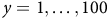
 $P(D \lt 1\mathrm{p}\mathrm{x})=94\mathrm{\%}$
when
$P(D \lt 1\mathrm{p}\mathrm{x})=94\mathrm{\%}$
when $d=50$
(see Table 1). As discussed in the previous paragraph, the likelihood of speciation between any pair of cells is controlled by the relative strengths of gene flow and different adaptive pressures between cells. When gene flow is low (but greater than zero; e.g.
$d=50$
(see Table 1). As discussed in the previous paragraph, the likelihood of speciation between any pair of cells is controlled by the relative strengths of gene flow and different adaptive pressures between cells. When gene flow is low (but greater than zero; e.g. $d=35$
; Figure S2j), speciation between cells will become the favoured outcome in cell-pairs even for those with low adaptive differentials (i.e. in regions with low
$d=35$
; Figure S2j), speciation between cells will become the favoured outcome in cell-pairs even for those with low adaptive differentials (i.e. in regions with low $\left|\dot{e}\right|$
). When dispersal ability is low, therefore, the importance of the magnitude of adaptive differentials between cells becomes less – most differentials will be sufficiently large to ensure speciation. The correlation between
$\left|\dot{e}\right|$
). When dispersal ability is low, therefore, the importance of the magnitude of adaptive differentials between cells becomes less – most differentials will be sufficiently large to ensure speciation. The correlation between $\left|\dot{e}\right|$
and
$\left|\dot{e}\right|$
and $\overline{{S}_{x}}$
is hence weaker when dispersal ability is low, as variation in
$\overline{{S}_{x}}$
is hence weaker when dispersal ability is low, as variation in $\left|\dot{e}\right|$
is more weakly tied to the prevalence of speciation.
$\left|\dot{e}\right|$
is more weakly tied to the prevalence of speciation.
Relationships between dispersion and environmental variability.
 $d$
= dispersion parameter.
$d$
= dispersion parameter. ${D}_{max}=240/d$
= maximum dispersion (px).
${D}_{max}=240/d$
= maximum dispersion (px). $r$
= Pearson’s correlation coefficient.
$r$
= Pearson’s correlation coefficient. $G$
= dimensionless dispersion-environment number.
$G$
= dimensionless dispersion-environment number.
Note: $\lambda =50$
(px).
$\lambda =50$
(px).
A feature of our simulation results is that correlation coefficients between $\left|\dot{e}\right|$
and
$\left|\dot{e}\right|$
and $\overline{{S}_{x}}$
are consistently very high (
$\overline{{S}_{x}}$
are consistently very high ( $r\ge 0.99$
) where
$r\ge 0.99$
) where $d$
is below a particular value (
$d$
is below a particular value ( $d\,\lesssim\, 25$
; i.e. high dispersal ability). As our experiments use arbitrary units, threshold values of
$d\,\lesssim\, 25$
; i.e. high dispersal ability). As our experiments use arbitrary units, threshold values of $d$
cannot be directly related to corresponding values in real-world datasets. To facilitate comparisons to the real world, we define a dimensionless parameter,
$d$
cannot be directly related to corresponding values in real-world datasets. To facilitate comparisons to the real world, we define a dimensionless parameter, $G$
, that incorporates the ratio of spatial and dispersal scales
$G$
, that incorporates the ratio of spatial and dispersal scales
 $$G = {\lambda \over {{D_{max}}}}.$$ ${D}_{max}$
is preferred here over mean displacement as it is, perhaps, more easily measurable or estimatable for real-world species (extant or extinct). It also captures the spatial range at which gene flow is possible in each time step. Values of
${D}_{max}$
is preferred here over mean displacement as it is, perhaps, more easily measurable or estimatable for real-world species (extant or extinct). It also captures the spatial range at which gene flow is possible in each time step. Values of $G$
for different dispersal parameters are shown in Table 1. When
$G$
for different dispersal parameters are shown in Table 1. When $G\,\lesssim\, 5$
,
$G\,\lesssim\, 5$
, $\left|\dot{e}\right|$
is strongly positively correlated with
$\left|\dot{e}\right|$
is strongly positively correlated with $\overline{{S}_{x}}$
.
$\overline{{S}_{x}}$
.
The African transect demonstrates that positive and significant correlations exist between species richness and derivatives of environmental variables at wavelengths $\lambda \,\gtrsim\, 200$
km. Inserting this value into Equation (4),
$\lambda \,\gtrsim\, 200$
km. Inserting this value into Equation (4), $G$
= 5 gives
$G$
= 5 gives ${D}_{max}$
=
${D}_{max}$
= $40$
km. As the maximum dispersal for avian species is likely to be higher than
$40$
km. As the maximum dispersal for avian species is likely to be higher than $40$
km (Bowman, Reference Bowman2003; Chu & Claramunt, Reference Chu and Claramunt2023; Sutherland et al. Reference Sutherland, Harestad, Price and Lertzman2000),
$40$
km (Bowman, Reference Bowman2003; Chu & Claramunt, Reference Chu and Claramunt2023; Sutherland et al. Reference Sutherland, Harestad, Price and Lertzman2000), $G$
is likely to be
$G$
is likely to be $\,\lesssim\, 5$
, and thus the recovered correlations fit the predictions of our model.
$\,\lesssim\, 5$
, and thus the recovered correlations fit the predictions of our model.
We note that when $d\ge 40$
in the simulations (i.e. dispersal ability is relatively low) correlation coefficients between
$d\ge 40$
in the simulations (i.e. dispersal ability is relatively low) correlation coefficients between $\left|\dot{e}\right|$
and
$\left|\dot{e}\right|$
and $\overline{{S}_{x}}$
are close to zero (Table 1; Figure 7). We interpret this result as an artefact of the integer parameterization of
$\overline{{S}_{x}}$
are close to zero (Table 1; Figure 7). We interpret this result as an artefact of the integer parameterization of $e$
in our study. As discussed above, in any pair of adjacent cells with differing
$e$
in our study. As discussed above, in any pair of adjacent cells with differing $e$
, speciation will be favoured if differential adaptive pressure arising from the difference in
$e$
, speciation will be favoured if differential adaptive pressure arising from the difference in $e$
outweighs the homogenization provided by gene flow. When dispersal ability is low, gene-flow is low, and hence the difference in
$e$
outweighs the homogenization provided by gene flow. When dispersal ability is low, gene-flow is low, and hence the difference in $e$
between cells required to favour speciation is also lowered. If dispersal ability is lowered sufficiently, the difference in
$e$
between cells required to favour speciation is also lowered. If dispersal ability is lowered sufficiently, the difference in $e$
between cells required to favour speciation may fall to being
$e$
between cells required to favour speciation may fall to being $\lt 1$
. Because
$\lt 1$
. Because $e$
is an integer (in the model), the lowest possible difference in
$e$
is an integer (in the model), the lowest possible difference in $e$
between adjacent cells in the
$e$
between adjacent cells in the $x$
-direction is 1, except where it is precisely zero; in our environment maps, adjacent cells in the
$x$
-direction is 1, except where it is precisely zero; in our environment maps, adjacent cells in the $x$
-direction with differences of
$x$
-direction with differences of $e$
of 0 occur only at minima and maxima. For this reason, in our experiments, there must exist a threshold level of dispersal ability below which all cell-pairs in the
$e$
of 0 occur only at minima and maxima. For this reason, in our experiments, there must exist a threshold level of dispersal ability below which all cell-pairs in the $x$
-direction will favour speciation (except the very few where the difference in
$x$
-direction will favour speciation (except the very few where the difference in $e$
is zero), and hence below which the correlation between
$e$
is zero), and hence below which the correlation between $\left|\dot{e}\right|$
and
$\left|\dot{e}\right|$
and $\overline{{S}_{x}}$
will be very close to zero. We infer that this threshold is between
$\overline{{S}_{x}}$
will be very close to zero. We infer that this threshold is between $d=35$
and
$d=35$
and $d=40$
px
$d=40$
px ${}^{-1}$
. In the real world, dispersal ability is of course different for different species, and
${}^{-1}$
. In the real world, dispersal ability is of course different for different species, and $e$
is not constrained to be an integer. While we infer that the near zero correlations at high
$e$
is not constrained to be an integer. While we infer that the near zero correlations at high $d$
are artefactual due to the integer parametrization, we contend that the less precipitous decreases in correlation where
$d$
are artefactual due to the integer parametrization, we contend that the less precipitous decreases in correlation where $d\ge 25$
(
$d\ge 25$
( $G\ge 5$
) are not artefacts, as our explanation for their origin does not depend on integer discretization. We expect that high correlations may be observed in real-world datasets between
$G\ge 5$
) are not artefacts, as our explanation for their origin does not depend on integer discretization. We expect that high correlations may be observed in real-world datasets between $\left|\dot{e}\right|$
and
$\left|\dot{e}\right|$
and $\overline{{S}_{x}}$
where
$\overline{{S}_{x}}$
where $G\,\lesssim\, 5$
, and that correlations could be expected to be lower when
$G\,\lesssim\, 5$
, and that correlations could be expected to be lower when $G\,\gtrsim\, 5$
.
$G\,\gtrsim\, 5$
.
4.b. Simplifications and future work
The simulations in this study assume that dispersal capacity is identically distributed for all organisms in each experiment (i.e. $d$
is a constant). This assumption has the obvious benefit of simplifying the assessment of contributions from different driving processes. While we make no claim that this assumption is precisely true in any real-world system, we note that dispersal capacity is frequently observed to be similar within broad clades of extant organisms (Ceresa et al. Reference Ceresa, Belda and Monrós2016; Matthysen, Reference Matthysen2012; Zera & Brisson, Reference Zera, Brisson, Clobert, Baguette, Benton and Bullock2012). Assuming a constant dispersal distribution may thus be a viable strategy for understanding speciation within many taxa. Similarly, we note that the frequency distribution of dispersal used in our simulations is similar to that of real-world extant organisms in that offspring tend to settle closer to parents, with decreasing frequency at increasing ranges (Matthysen, Reference Matthysen2012; Nathan et al. Reference Nathan, Schurr, Spiegel, Steinitz, Trakhtenbrot and Tsoar2008; Nathan & Muller-Landau, Reference Nathan and Muller-Landau2000). The African avian transect examined in this study serves as a single example, focusing on one taxon in a region chosen for its relatively stable environmental conditions over recent geological timescales. This stability facilitates comparisons with models that seek to isolate contributions to species richness from spatial environmental change, as we do here. Further and broader analyses of different taxa and transects are beyond the scope of this preliminary study, but are likely to prove fruitful for interpreting the spatial distributions of extant and extinct organisms. An obvious next step is to consider how we might relate the fossil record directly to results from such simulations, taking into account preservation potential and biases (sensu Alroy et al. Reference Alroy, Marshall, Bambach, Bezusko, Foote, Fürsich, Hansen, Holland, Ivany, Jablonski, Jacobs, Jones, Kosnik, Lidgard, Low, Miller, Novack-Gottshall, Olszewski, Patzkowsky and Webber2001).
$d$
is a constant). This assumption has the obvious benefit of simplifying the assessment of contributions from different driving processes. While we make no claim that this assumption is precisely true in any real-world system, we note that dispersal capacity is frequently observed to be similar within broad clades of extant organisms (Ceresa et al. Reference Ceresa, Belda and Monrós2016; Matthysen, Reference Matthysen2012; Zera & Brisson, Reference Zera, Brisson, Clobert, Baguette, Benton and Bullock2012). Assuming a constant dispersal distribution may thus be a viable strategy for understanding speciation within many taxa. Similarly, we note that the frequency distribution of dispersal used in our simulations is similar to that of real-world extant organisms in that offspring tend to settle closer to parents, with decreasing frequency at increasing ranges (Matthysen, Reference Matthysen2012; Nathan et al. Reference Nathan, Schurr, Spiegel, Steinitz, Trakhtenbrot and Tsoar2008; Nathan & Muller-Landau, Reference Nathan and Muller-Landau2000). The African avian transect examined in this study serves as a single example, focusing on one taxon in a region chosen for its relatively stable environmental conditions over recent geological timescales. This stability facilitates comparisons with models that seek to isolate contributions to species richness from spatial environmental change, as we do here. Further and broader analyses of different taxa and transects are beyond the scope of this preliminary study, but are likely to prove fruitful for interpreting the spatial distributions of extant and extinct organisms. An obvious next step is to consider how we might relate the fossil record directly to results from such simulations, taking into account preservation potential and biases (sensu Alroy et al. Reference Alroy, Marshall, Bambach, Bezusko, Foote, Fürsich, Hansen, Holland, Ivany, Jablonski, Jacobs, Jones, Kosnik, Lidgard, Low, Miller, Novack-Gottshall, Olszewski, Patzkowsky and Webber2001).
First, we suggest that combining experiments of the type presented in this paper with knowledge of dispersal and environmental variability in the real world could be a way to establish likely distributions of contemporary and ancient biodiversity. Doing so could provide opportunities to develop predictive capabilities to determine species richness across scales. Conversely, interpreting palaeontological records with this framework in mind may support the understanding of environmental change in space and time and quantification of associated uncertainties. A better understanding of linkages could aid in environmental reconstruction from biodiversity patterns. Secondly, a more nuanced understanding of the relationship between spatial structure and biodiversity might be obtained by allowing dispersal ability to vary under genetic control in the eco-evolutionary experiments. Thirdly, an obvious extension is to examine the impacts of more complicated spatio-temporal environmental change on species richness. Future work could incorporate multiple taxa across diverse regions on Earth and make use of insights from dynamic modelling and the geological record to incorporate temporal variability, for instance. Finally, incorporating taxa that occupy similar ranges but are evolutionarily distant, and have different modes of dispersal, could establish an understanding of how such traits impact relationships between environments and biodiversity.
5. Conclusions
By repeatedly running the ‘experiment of life’ with models of evolution that incorporate random dispersal, mutation and a static environment, statistical insights into the relationships between species richness and spatial environmental variability are established. The results show that, in such systems, species richness should be expected to correlate with the spatial rate of change (strictly, the spatial derivative) of the environment. The strength of the correlation is principally dependent on two factors: the dispersal ability of the organisms and the spatial scale of environmental variables. The role of these factors can be understood through established ecological and evolutionary mechanisms. We demonstrate how that relationship can help to contextualize a transect of real-world present-day species data, demonstrating that, under certain circumstances, our findings are applicable outside the realm of simulation. The results suggest that such an approach may be useful for contextualizing the fossil record or for using the fossil record to reconstruct past environments. When the scale of environmental change is sufficiently small compared to the distance organisms can disperse, the scale of environmental change can reliably predict the distribution of species richness across an environment. We emphasize that these relationships might not be apparent in single experiments or observations generated from sparse fossil assemblages, for instance, because of the randomness of biological evolution. Instead, it is the statistical properties that arise from running many experiments that provided the information needed to identify the relationships and generate the predictions presented in this study. We suggest that it could be fruitful to establish statistical relationships between rates of environmental change and species richness across scales in the modern and ancient real world.
Supplementary material
The supplementary material for this article can be found at https://doi.org/10.1017/S0016756825100502.
Acknowledgements
Thanks to Francois van Schalkwyk for the HPC support and Dr Sameer Bansal for the coding review.
Financial support
G.B. is supported by the Natural Environment Research Council (NE/S007415/1).
Competing interests
The authors declare none.
AI contributions to research content
The authors declare that large language models were used, when necessary, to assist in debugging the Python code.


 Open access