
1.1 Introduction
When it comes to analyzing data, contemporary analysts have an embarrassment of riches. Principal components and factor analysis can help reduce many variables into few. Kernel density estimation can approximate the distributions of variables. Regression regularization, Bayes factors or AIC selection methods, decision trees, and other machine learning methods can assist in choosing variables to predict outcomes. These techniques have great value in summarizing data, estimating variable values, or exploratory analysis. Yet when researchers have specified models in advance that contain substantively driven hypotheses and their desire is to estimate and test these hypothesized structures and their causal inferences, many of these techniques fall short. Causal inference seeks to assess the causal relations between variables rather than to summarize or predict variables. The plausibility of causal inferences is boosted by randomized treatments or interventions that lessen the threats of confounders that affect the explanatory and outcome variables. But randomized interventions are not always feasible. When the target causal variables (treatments) are not randomized, researchers need to include control variables or take into account variables that, if ignored, would bias the estimates of effects of the causal variables.
In practice, there are at least two common problems to introducing control variables: (1) impromptu specification of outcome equations and (2) ignoring measurement error. Consider impromptu specifications first. Researchers often target one variable and its effects on a dependent variable. They recognize the need to control variables that could distort the estimates. Often researchers’ inclusion of control variables (covariates) is based on intuition, impressions, and opinions in combination with bivariate correlations of whether the included covariates are associated with the causal and dependent variables. This is reinforced by a belief that adding more control variables to predict an outcome is a conservative way to proceed in that controlling for more variables is more likely to minimize or reduce sources of confounding that could bias the estimates of the target causal variable on the outcome. However, this common orientation can yield misleading results.
To illustrate, I present a hypothetical example where X1 is the target causal variable and Y1 is the outcome variable. The researcher suspects that Y2, another pre-outcome variable, is correlated with both X1 and Y1 and might confound their relationship. Checking the correlation matrix of the three variables, the researcher generates Table 1.1. As suspected, Y2 correlates with both the target variable X1 and the outcome variable Y1. Indeed, the Y2 correlation with Y1 is 0.584, which is higher than the correlation of Y1 with X1, which is 0.505. Thus, the researcher runs the Ordinary Least Squares (OLS) regression of Y1 on both Y2 and X1 and contrasts this with the regression of Y1 on only X1. Table 1.2 gives the results.
| Y1 | Y2 | X1 | ||
| Y1 | 1.000 | |||
| Y2 | 0.584 | 1.000 | ||
| X1 | 0.505 | 0.522 | 1.00 |
| (1) | (2) | |
| Y1 | Y1 | |
| X1 | 0.503 | 0.274 |
| (0.004) | (0.004) | |
| Y2 | 0.354 | |
| (0.003) | ||
| R-squared | 0.255 | 0.396 |
Standard errors are in parentheses.
The coefficient of X1 is positive and significant in both regressions. Column (2) shows that when the researcher regresses Y1 on X1 and Y2, they both have positive coefficients. The coefficient of X1 is roughly half the magnitude in column (2) versus column (1). In addition, the R-squared of 0.396 in column (2) is notably larger than the 0.255 R-squared in column (1). Based on the positive and significant effects of X1 and Y2 and the much higher R-squared in column (2), the regression in the second column appears superior to that in column (1).
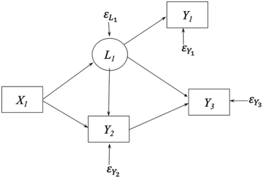
But appearances are deceiving. Figure 1.1 is the path diagram of the data generating model (DGM) of these data.Footnote 1 Chapter 2 gives a detailed description of the symbols of path diagrams. Here I briefly describe their meaning in Figure 1.1. The circles represent latent variables L1 and L2, which are variables that are unobserved in the data yet have causal influence on Y1, Y2, and X1 where these latter observed variables are enclosed in boxes. The εs are the error terms for the observed variables and represent all other influences on their respective variables that are not part of the model. The single-headed arrows represent the causal influence of the variable at the base of the arrow on the variable to which it points.
Data generating model for X1, X2, and Y1.
The population parameters of the DGM set the X1 ➔ Y1 path to 0.5, while the rest of the parameter values of the DGM are in Appendix in the Stata or R commands that generated the data. Note that the 0.5 parameter is close to the estimate of the effect of X1 on Y1 in column (1) where Y2 is omitted. Indeed, regressing Y1 on only X1 is the correct way to recover the causal effect of X1 on Y1. Furthermore, Y2 has no direct or indirect effect on Y1 despite the positive coefficient in column (2) of Table 1.2. The impromptu specification is badly misleading. Intuition and the correlation matrix suggested that Y2 should be included in the Y1 equation, and by so doing, it misled us into thinking that Y2 had a positive direct causal effect on Y1 and that X1’s impact on Y1 was almost half its true magnitude. And notice that this example departs from the traditional spurious relation example where two variables both depend on a third variable that creates an association between them. Here a partial association between two variables is created by including it in the regression.
This example illustrates the broader problem of the widespread practice of impromptu specifications. Researchers might believe that they are being cautious when they test the effects of a causal variable on an outcome by liberally including many control variables in an equation. As this example illustrates and the literature on “bad controls” shows, this is not true (e.g., see Angrist & Pischke, Reference Angrist and Pischke2009; Cinelli et al., Reference Cinelli, Forney and Pearl2022; Schisterman, Cole, & Platt, Reference Schisterman, Cole and Platt2009). It points to the need to specify one (or more) models for the outcome, treatment variable, and other variables in the model. There is no guarantee of having a correct model; however, by giving more thought to plausible structures, the chances are improved of getting closer to the actual DGM. In addition, there is no reason not to consider several different structures for the same variables to see which best approximates the associations of the observed variables. This is especially true when a consensus is lacking on a true model or if there are competing models in the literature.
Structural equation models (SEMs) start with the researcher specifying a model that incorporates the analysts’ best understanding of the relationships between all variables in the model. The model specification draws on past research, substantive expertise, and speculations, so it is challenging for someone lacking knowledge of the subject matter to use SEMs. Indeed, the specification of the model is the first step in modeling and specification requires subject matter expertise from the analysts or collaborators. Systematic thinking combined with substantive expertise can catch specification errors that go unnoticed with impromptu specifications.
A second common problem in empirical research is ignoring the measurement error present in explanatory variables. Many social, economic, and behavioral science variables such as socioeconomic status, depression, happiness, disposable income, inflationary expectations, or ability are virtually impossible to measure without error. Other variables such as economic measures of unemployment or inflation, or health measures such as blood pressure, LDL cholesterol, or heart rate are less abstract, but they too suffer from measurement errors. Yet it is common to enter these and other variables into outcome equations and to treat them as if they were error-free. In some cases, analysts acknowledge, but do not take account of, the measurement error. When measurement errors in explanatory variables are ignored, researchers are essentially introducing unobserved confounders.
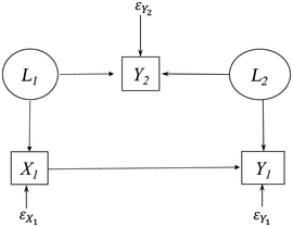
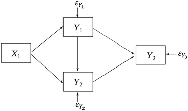
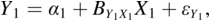
To demonstrate this claim, consider Figure 1.2, which is a path diagram of the relationships among four observed variables. All relations depicted are between observed variables which implicitly assume no measurement errors. To illustrate why measurement error implies confounding, assume that Y1 contains measurement error and that L1 is the latent variable underlying it that is free of error. Figure 1.3 is the resulting path diagram. The L1 ➔ Y1 relation represents that the latent variable L1 influences its indicator Y1. The measurement error in Y1 is captured by  . The
. The  is the collection of other variables that affect L1 but are not in the model. Note that L1 appears in the Figure 1.3 in place of where Y1 was in Figure 1.2, and including it allows me to explicitly account for the measurement error.
Path diagram of four variables ignoring measurement error.
Path diagram with measurement error in Y1.

Figure 1.3 illustrates how measurement error implies unmeasured confounders. Unmeasured confounders are omitted variables that influence both an explanatory variable and the outcome variable in an equation. If I ignore measurement error in Y1 by using the model in Figure 1.2, then Figure 1.3 shows that L1 is an unmeasured confounder in the Y3 equation. Namely, the omitted L1 directly influences Y1 and Y3, and this could create a spurious relation between Y3 and Y1 in Figure 1.2. However, Figure 1.3 shows there is no relation between them when L1 is included in the model. Furthermore, even if X1 were perfectly measured, its coefficient estimate is likely to be biased by the measurement error in Y1 in the Y3 equation. In addition, ignoring measurement error in Y1 in the Y2 equation creates biased estimates because L1, not Y1, directly influences Y2 and the failure to control measurement error in Y1 creates bias in the coefficients of Y1 and X1. As this example shows, ignoring measurement error in an explanatory variable (covariate) often results in biased estimates not only of the variable with error but even of other covariates that are perfectly measured.
Treating explanatory variables as if they were essentially error-free is widespread across disciplines. By ignoring measurement errors, analysts risk biased estimates of key causal variables. The target causal variable could even have negligible measurement error, but if other correlated covariates have measurement error, it can spoil the target causal variable’s coefficient estimate (Bollen, Reference Bollen1989b).
This same problem creates difficulties for a popular approach to causal inference based on modeling assignment to treatments and using propensity scores (Rosenbaum & Rubin, Reference Rosenbaum and Rubin1983, Reference Rosenbaum and Rubin1984). These procedures assume no unobserved confounders that affect both the assignment to treatment and the outcome. Yet, if the covariates included in the assignment equation contain measurement error, then the latent variable that underlies the measure remains a confounder as illustrated above. To the degree that the assignment equation and the outcome equation introduce many covariates as controls, they also could be subject to the problems raised by impromptu specifications that I previously described (Pearl, Reference Pearl2009b, Reference Pearl2009c).
A related measurement problem is to include multiple measures of the same latent variable as separate covariates in an equation. For example, researchers might be interested in the effects of anxiety on depression. Instead of forming a latent anxiety variable, they might include indicators of anxiety as distinct causal variables on the right-hand-side (RHS) of a depression equation. As these indicators are measures of the same latent variable, their coefficients are likely to depart from the actual effect of the latent anxiety variable on depression. This is due to both the measurement error in each indicator and the potential multicollinearity between them. Alternatively, a researcher might include an “anxiety scale” composed of the anxiety indicators to replace the latent variable of anxiety. Unfortunately, the weighted sum of the indicators that forms the anxiety scale is not the same as the latent anxiety variable. It contains measurement error, and as I have explained, measurement error generally biases coefficient estimates of both the target variable and the control variables. Both these situations – incorporating the indicators as separate variables or including weighted composite of the indicators – exemplify both the impromptu specification and the neglect of measurement error problems that I have described. A more systematic approach would use the multiple measures as indicators of a latent variable and have the latent variable as an explanatory variable in the outcome equation.
Fortunately, SEMs provide tools to address these problems. With model specification as the first step, SEM encourages researchers to stipulate the relationships between variables more completely. This includes building measurement models that permit researchers to take account of measurement errors in the covariates. Random measurement errors are controllable by incorporating estimates of measurement reliability or by using multiple indicators of latent variables into SEMs as I discuss in Chapter 5. Thus, SEMs provide a tool to address the widespread problems of impromptu specifications and measurement error in covariates, and by so doing, they can improve causal inferences.
1.2 What Are Structural Equation Models (SEMs)?
So far, I have given SEM examples and described their use in addressing impromptu specifications and taking account of measurement errors. Yet, I have not directly defined SEMs. Though a consensus on the definition of SEMs is elusive, in this section I sketch the meaning of SEMs as I use them in this book. I begin by defining each term in “structural equation models.”
1.2.1 Structural
Koopmans and Reiersøl (Reference Koopmans and Reiersol1950) had an early discussion of the meaning of structural that remains relevant today:
In many fields the objective of the investigator’s inquisitiveness is not just a “population” in the sense of a distribution of observable variables, but a physical structure projected behind this distribution, by which the latter is thought to be generated. The word “physical” is used merely to convey that the structure concept is based on the investigator’s ideas as to the “explanation” or “formation” of the phenomena studied, briefly, on his theory of the phenomena, whether they are classified as physical in the literal sense, biological, psychological, sociological, economic or otherwise.
Koopmans and Reiersøl (Reference Koopmans and Reiersol1950) make clear that structure is not equivalent to the distribution of observed variables as might be the focal point of a statistics perspective. Rather, structure is the explanation of what creates the distributions. In other words, it is the set of causal and noncausal relations among the variables and their errors that result in the distributions of the variables researchers observe. Koopmans and Reiersøl also make clear that the concept of structure extends beyond that of physical phenomena to structures in the biological, social, economic, and behavioral sciences.
Though Sewall Wright (Reference Wright1921, 1934) used terms such as “path diagrams” and “path coefficients,” his writings and applications capture a crucial aspect of structural as it relates to causal relations of interest. Wright saw path diagrams as incorporating the causal assumptions of researchers and the path coefficients were measures of causal effects. Goldberger (Reference Goldberger1972, p. 979) succinctly captures the close connection of structural and causal: “By structural equation models I refer to stochastic models in which each equation represents a causal link, rather than a mere empirical association.”
Other connotations are sometimes added to structural. For instance, Duncan (Reference Duncan1975, p. 151) described structural coefficients as “unmixed, invariant, and autonomous.” Similarly, Goldberger (Reference Goldberger1973, p. 6) described structural parameters as “stable.” However, if these parameters can differ over time, across groups, or between individuals, the rationale of requiring invariance and stability as essential to structural seems hard to justify. Furthermore, parameters need not be constant. For instance, in Bayesian analysis the coefficient parameters have prior and posterior distributions rather than a constant value, and these parameters are still structural (Lee, Reference Lee2007).
Nonetheless, at its core, structural means causal. Whether invariance and stability of these parameters hold are instead distinct research questions. This does not mean that all parameters that are part of a structural equation model describe causal relations. The structural coefficients that correspond to the direct and indirect relations between latent and/or observed variables are parameters that capture the causal relations between variables. However, many models include the means, intercepts, variances, and covariances of errors or of exogenous variables as model parameters.Footnote 2 The means, intercepts, variances, and covariances from SEMs are structural parameters in that they are parameters from a SEM, but these parameters do not give cause–effect relationships.
Pulling these ideas together, the “structural” in SEM implies that a model contains at least one causal relation. Though the coefficients are most closely tied to the causal effect of one variable on another, in practice all parameters from a SEM are often called structural parameters, even though some such parameters are variances, covariances, or intercepts that are less closely linked to giving causal effects.
1.2.2 Equation
Equation is the second term in SEM. As the name suggests, an equation equates a left-hand and right-hand side expression of variables and/or constants. As an illustration, L2 = α2 + B21L1 + ε2 is an equation that shows the latent variable L2 equal to a constant α2 plus another constant B21 times another latent variable L1 plus a random error variable ε2. Written as such, this is an algebraic equation that could be manipulated to solve for L1 or any other variable or constant alone on the left-hand side (LHS). But this is where the term “structural” and the joint term “structural equation” become important. By convention, the LHS of a structural equation is a dependent variable receiving the causal effects of the right-hand side (RHS) variables. L1 causes L2; thus, L1’s placement on the RHS is a causal assumption, not an arbitrary algebraic placement in the equation.
Another point is that there are two major kinds of equations in SEM. One has an explicit functional form while the other does not specify the functional form. The example in the preceding paragraph, L2 = α2 + B21L1 + ε2, is an explicit functional form that is linear in the variables and linear in the parameters. Alternatively, L2 = f(L1, ε2) includes the same variables, but the functional form is not explicit. The latter is sometimes called a nonparametric structural equation, and these are associated with Directed Acyclic Graphs (DAGs) (Pearl, Reference Pearl2010), though see Bollen and Pearl (Reference Bollen and Pearl2013, pp. 315–316). Although the book has some discussion of DAGs, much of the material covers equations with explicit functional forms. This does not mean SEMs with explicit functional forms are “linear Gaussian” as is sometimes claimed. I discuss this point later in the chapter in the section on “Myths about SEMs.”
1.2.3 Model
Model is the last term in SEMs. To define models, it helps to provide some background. Start by considering the objects or units of analysis, whether they are individuals, groups, counties, nations, or some other unit. These units have properties. If individuals are the object of study, properties would include things such as their age, anxiety, intelligence, or socioeconomic status. Or if family is the unit, family size, age distribution, or single-headed household are examples of properties. Hypotheses are statements or claims that link two or more properties, often in the form of causal relationships, and a theory consists of one or more hypotheses.
In the context of SEMs, variables represent properties, and the variables are either observed variables that are included in the dataset, or latent variables that are not (Bollen, Reference Bollen2002; Bollen & Hoyle, Reference Bollen and Hoyle2023). The hypotheses link properties and the variables that stand for these properties in the model. Thus, the hypothesized links are between latent variables, observed variables, or a combination of the two. For instance, a hypothesis might claim that anxiety causes depressed affect where both variables are latent. Or the hypothesis might claim that the level of depressed affect drives the responses to several observed variable indicators (e.g., responses to a question that asks the degree to which a respondent “feels sad”). This latter hypothesis is about measurement or the relation between a latent variable and its observed indicators.
The properties, hypotheses, and the theory that contains them are abstract ideas. Models are formal representations of these abstract ideas where variables stand for properties, the links between variables signify the hypotheses, and the full model is the counterpart to the theory connecting hypotheses.
The two major ways to represent a model in SEMs are with equations and with path diagrams. The first section of this chapter introduced path diagram examples, and Chapter 2 describes the diagram symbols in more detail. However, there is a close relation between representing the model with the path diagrams or with the equations. To illustrate, consider Figure 1.2. The equations that correspond to the path diagram are:


The causal variables are on the RHS of each equation for Y1 to Y3. Depending on the equation, the Ys are either dependent or causal variables in the model. In the first equation, for example, Y1 is the dependent variable, while in the second equation Y1 is a cause of Y2. Though I did not show the intercepts in the path diagram, this is also possible (see Chapter 2).
These two ways of representing the same model are a convenient feature of SEMs. Researchers familiar with SEMs can move from the path diagram to equations as I illustrated, or vice versa. Many scientists find the path diagrams as a convenient and quick way to comprehend the whole model including the system of relationships between variables, as well as to spot omissions of direct effects or correlations among variables.
1.2.4 Summary
Addressing the question of what are structural equation models was the goal of this section. I discussed each term in the subsections; however, I can combine these ideas into a briefer full definition of structural equation models. Structural equation models are formal depictions of the relationships between a set of variables. The relationships originate from subject matter hypotheses or speculations that specify causal connections, noncausal associations, or lack of associations between variables. The variables can be latent or observed. Causal effects can be direct or indirect. The representation of the model is in a set of equations and assumptions or in a path diagram with the equivalent information. Furthermore, at least some parts of the model are subject to rejection when compared to empirical data. In contrast, researchers can never prove a model’s validity even if it fits the data well.
1.2.5 SEMs as a General Statistical Model
The last section defined SEMs as a modeling approach to incorporate, test, and assess causal assumptions. In other words, SEMs are a tool for causal inference. From another perspective, structural equation modeling provides a general statistical model that incorporates many of the most widely used statistical models. Multiple regression, multivariate regression, simultaneous equation models, ANOVA, ANCOVA, factor analysis, binary and ordinal probit regression, fixed and random effects regressions, and latent growth curves are examples of statistical models that are available by placing restrictions on the full latent variable SEM that I present. As a statistical model capable of including latent and observed variables, multiple indicators and measurement errors, and binary and ordinal variables among other features, it is easy to understand how this viewpoint of structural equation modeling as a general statistical model has spread.
Realization of the generality of SEMs is not a problem per se. What is a problem is that in applications, analysts are not always clear as to when they are employing SEMs for causal inferences versus when they are taking advantage of it as a general statistical model with another goal in mind. If the investigator is testing explanatory hypotheses, interventions, or treatment effects, it seems likely that causal inferences are the goal. But readers should be aware of this distinction.
1.3 Origins of Structural Equation Models (SEMs)
In 1904 English psychologist Charles Spearman (Reference Spearman1904) published an article in the American Journal of Psychology hypothesizing that a single “General Intelligence” factor underlay the performance on numerous different tests of students. In 1918, American geneticist and statistician Sewall Wright (Reference Wright1918) empirically examined whether a single size factor underlay the bone sizes of different body parts of rabbits.Footnote 3 Spearman’s (Reference Spearman1904) focus was ability tests, and Wright’s (Reference Wright1918) was biological measures, but both used empirical methods to detect latent variables or factors based on the associations of observed variables created by the underlying latent variables.
Spearman’s attention was on the impact of a latent variable or factors on its observed measures. Sewall Wright’s (Reference Wright1918) initial study had a similar purpose, but Wright (Reference Wright1921, Reference Wright1925, Reference Wright1934, Reference Wright1960) went on to develop path analysis that uses graphs of variables linked by single-headed arrows to depict hypothesized causal relations and double-headed arrows between variables to show unanalyzed correlations. In some path analysis models Wright (Reference Wright1918, Reference Wright1921, Reference Wright1925, Reference Wright1934) included both latent and observed variables that enabled the study of postulated variables for which error-free versions were unavailable. Wright also pioneered the analysis of direct, indirect, and total effects between variables with mediation analysis. In other words, Wright considered a broader class of models than factor analysis.
I began this section with Charles Spearman and Sewall Wright because if we seek the origins of structural equation models (SEMs), these two scholars are prime candidates. Spearman (Reference Spearman1904) and the psychometricians who followed developed factor analysis that reduces a large set of observed variables into fewer latent variables. Wright pioneered the use of graphs or diagrams to capture the assumed causal and noncausal relations among variables, both observed and latent.
Spearman and Wright also are good choices as founders of SEM because key aspects of their approaches continue today. For one thing, model specifications were based on subject matter expertise. Spearman (Reference Spearman1904) hypothesized a general intelligence factor (latent variable) that could explain the association of performance on a variety of tests. Factor analysis was a means to check this hypothesis. Wright (Reference Wright1918) wanted to determine whether a general size factor might explain the bones sizes of different body parts in rabbits. They both hypothesized latent variables to explain observable characteristics and devised empirical techniques to test these hypotheses. Furthermore, Wright developed methods to analyze the direct, indirect, and total effects of variables with each other.
Like these early applications, contemporary SEM research depends on subject matter expertise to formulate models that best represent the understanding of the phenomena under study. Without such knowledge, the first step of model specification is incomplete. SEM is not based on supplying a list of variables and having an algorithm determine how these variables are related. Rather, the starting point is a model that incorporates researchers’ best substantive expertise and speculations about the relationships between variables. Part of the specification is hypothesizing causal relations and the lack thereof among variables. Causal assumptions are the key input to causal inferences derived from SEMs. Though researchers cannot prove causal relations, they can harvest empirical information that is consistent or inconsistent with them. When inconsistent, it raises questions about the causal assumptions that went into the model. When consistent, the model and causal assumptions survive this test. But this does not preclude finding a model that better explains the data or the rejection of the model if applied to new data.
A seemingly cautious approach to making causal assumptions is to let everything be related to everything else and to “let the data speak for itself.” The Achilles’ heel of this approach is that such a model is underidentified. I will go over the meaning of identification in more detail throughout the book, but in brief underidentified means that the true parameter values are indistinguishable from false ones. Both false and true values would be consistent with the data, and analysts could not determine which is which. Determining whether it is possible to find unique values of the parameters from a model is the question of model identification, and this is key to SEMs as I highlight in the chapters that follow.
Wright was aware of the identification problem as he worked with a variety of examples and attempted to solve for the path coefficients of the model from the correlations (covariances) of the observed variables. In some models, he found that there were multiple ways to solve for the same parameter. In contemporary terms, these are overidentified parameters, when there is more than enough information to identify the parameters. Wright sometimes compared the different sample solution estimates for the same parameter as an informal test of the model. After all, if the model were true, then the different solutions should be within sampling fluctuations of each other. If they were not, then this was evidence against the specification of the model.
Overidentification tests continue to be useful diagnostics for evaluating model specifications, though the tests are in new forms. The full information maximum likelihood estimatorFootnote 4 that I discuss in several chapters has a chi-square likelihood ratio test that compares the model implied means, variances, and covariances to the population means, variances, and covariances of the observed variables (Jöreskog, Reference Jöreskog1977). In overidentified models, a poor match between these quantities in the sample casts doubt on the model specification. Various functions of this same chi-square test statistic enter many fit indexes to help to assess model fit. But the chi-square test and fit indexes have their basis in overidentification tests. Later in the book, I discuss a model implied instrumental variable approach to SEMs (Bollen, Reference Bollen1996b). Here too there are overidentification tests to assess whether the different ways to estimate overidentified parameters are within sampling fluctuations. Thus, overidentification tests and the fit indexes that build on them provide important checks on the accuracy of models and their equations.
Wright’s (Reference Wright1921) introduction of the path diagram was an innovative, easy-to-grasp representation of the set of relationships assumed by researchers. I previewed path diagrams earlier in this chapter and will present path diagrams in more detail in Chapter 2. Path diagrams make clear the causal assumptions of researchers where direct, indirect, total, and noncausal relationships are readily viewable. They allow latent, observed, and error variables in a model. Furthermore, the path diagram is translatable into a series of equations and vice versa. In other words, the path diagram or the system of equations represent the same model, and researchers can use either or both.Footnote 5
It took until the 1960s and 1970s for Wright’s path analysis to take off in the social, economic, and behavioral sciences (Blalock, Reference Blalock1969; Duncan, Reference Duncan1966; Goldberger, Reference Goldberger1972; Werts & Linn, Reference Werts and Linn1970). The early applications were like Wright’s in that they were individual examples with example-specific solutions. The main exception was in econometrics where general simultaneous equation models were widely known (e.g., Goldberger, Reference Goldberger1964).Footnote 6 The simultaneous equations were multiequation models represented with a general matrix equation that could accommodate specific examples. This permitted the development of general rules of identification, estimation, and diagnostics tests. Their major limitation was the dominant assumption that the variables were measured without error. This meant that simultaneous equation models were not applicable in the presence of multiple indicators, latent variables, or measurement error.
A turning point in the history of SEMs were general multiequation models that included relationships for both latent and observed variables, multiple indicators, and measurement errors. These emerged in the 1960s and 1970s with the best known being the LISREL model (Jöreskog, Reference Jöreskog1973; Jöreskog & van Thillo, Reference Joreskog and van Thillo1972; Keesling, Reference Keesling1972; Wiley, Reference Wiley1973). The rise of the LISREL and similar models were general enough to include simultaneous equation models and factor analysis models as special cases. It also meant that researchers did not need customized solutions for each individual example that they developed. Furthermore, the LISREL software that accompanied the LISREL model and other SEM software allowed researchers to estimate and test their specific models using general algorithms.
The origin of SEMs and their spread in the 1960s and 1970s are only part of their story and the numerous scientists who have advanced their development. SEMs have spread to even more disciplines; have become more general; include numerous estimators, fit statistics, and diagnostics; and have a wide variety of software programs to implement them. For more complete histories and contemporary developments, see, for example, Goldberger (Reference Goldberger1972), Bielby and Hauser (Reference Bielby and Hauser1977), Bollen (Reference Bollen1989b, pp. 1–9), Bollen et al. (Reference Bollen, Fisher, Lilly, Brehm, Luo, Martinez and Ye2022b), and Matsueda (Reference Matsueda2023).
1.4 Myths about SEMS
Ever since Sewall Wright (Reference Wright1918, Reference Wright1921) laid the foundations of SEMs and DAGs, myths about them have propagated and persisted. Here I highlight several from Bollen and Pearl (Reference Bollen and Pearl2013) plus another not previously discussed.
1.4.1 Myth #1 SEMs Aim to Establish Causal Relations from Associations Alone
This widespread myth holds that users of SEMs believe that the presence or absence of associations and partial associations among variables in regression equations, simultaneous equation models, or factor analyses is sufficient to yield causal relations. These beliefs are more characteristic of critics of SEMs (Baumrind, Reference Baumrind1983, p. 103; De Leeuw, Reference De Leeuw1985, p. 372; Freedman, Reference Freedman1987, Reference Freedman2004, p. 2; Guttman, Reference Guttman1977, p. 97; Sobel, Reference Sobel2008) than the presenters of SEMs (Bollen, Reference Bollen1989b, pp. 40–79; Duncan, Reference Duncan1975, Reference Duncan1966; James, Mulaik, & Brett, Reference James, Mulaik and Brett1982; Mulaik, Reference Mulaik2009).
A quote from Sewall Wright (Reference Wright1921, p. 557) is perhaps the best way to reveal the contradiction: “The method [of path analysis] depends on the combination of knowledge of the degrees of correlation among the variables in a system with such knowledge as may be possessed of the causal relations. In cases in which the causal relations are uncertain the method can be used to find the logical consequences of any particular hypothesis in regard to them.” In other words, researchers input causal assumptions to build their SEMs. They do not derive causality solely by empirical means. As I noted earlier, the causal assumptions come from subject matter expertise, hypotheses, research designs, temporal priority, prior studies, and speculations that in turn lead to the specified models. Furthermore, empirical evidence can contradict these causal assumptions but cannot prove them to be valid.
Bollen and Pearl (Reference Bollen and Pearl2013) distinguish between weak and strong causal assumptions. The weak causal assumptions are those that specify relationships between pairs of variables without giving a specific numerical value of the parameter other than to claim that it is nonzero and perhaps to say that it is positive or that it is negative. For instance, suppose a coefficient is the parameter. A weak causal assumption states that X1 causes Y1 or it could claim that the coefficient is nonzero. This is a weak causal assumption because an infinite number of values of the coefficient are consistent with the causal assumption and only a zero coefficient contradicts it. Strong causal assumptions state that relationships between two variables are zero or some other constant value. Returning to the example, a causal assumption that X1 does not cause Y1 implies only one population coefficient value, that is, zero. An infinite number of other coefficient values contradict this causal assumption. Another example of a strong causal assumption is to specify that the population covariance or correlation of two error variables in a model is zero. A population value of zero is the only value that satisfies this strong causal assumption.
Bollen and Pearl (Reference Bollen and Pearl2013, p. 309) summarize the role of causality in SEMs as follows:
SEM is an inference engine that takes in two inputs, qualitative causal assumptions and empirical data, and derives two logical consequences of these inputs: quantitative causal conclusions and statistical measures of fit for the testable implications of the assumptions. Failure to fit the data casts doubt on the strong causal assumptions of zero coefficients or zero covariances and guides the researcher to diagnose or repair the structural misspecifications. Fitting the data does not “prove” the causal assumptions, but it makes them tentatively more plausible. Any such positive results need to be replicated and to withstand the criticisms of researchers who suggest other models for the same data.
1.4.2 Myth #2 SEMs and Regression Are Essentially Equivalent
Another mischaracterization of SEMs is the claim that they are essentially equivalent to regression equations whether they are regressions with observed or latent variables on the LHS and observed or latent variables on the RHS. Holland (Reference Holland1995, p. 54) provides a representative quote when the variables are observed:
I am speaking, of course, about the equation: y = a + bx + ε. What does it mean? The only meaning I have ever determined for such an equation is that it is a shorthand way of describing the conditional distribution of y given x. It says that the conditional expectation of y given x, E(y | x), is a + bx …).
Berk (Reference Berk2004, p. 191) among others gives a similar critique. The suggestion is that regression equations are no different than structural equations.
To respond to this critique, it helps to know that regression equations can serve several purposes. If I consider a single equation with LHS variable Y and two RHS variables of X1 and X2, then I can write a regression equation of

The conditional distribution Y given X1 and X2 is

as suggested by Holland (Reference Holland1995). But as a regression equation, I can just as easily write,

with a conditional distribution of X1 given Υ and X2 as

where  , and
, and  .
.
As regression equations with no other assumptions, I can place any of the variables on the LHS and solve for the RHS. These lead to different conditional expectation equations because the LHS variable differs. I can view these as prediction equations for the LHS variable, or I can use them as summary descriptive statistics of the predicted mean of the LHS variable. However, if the equation with Y on the LHS is a structural equation, then Y is an outcome variable, and the analyst is assuming that X1 and X2 are causes of Y. I can write a structural equation that puts X1 on the LHS, but it need not be equivalent to the preceding X1 equation. Instead, such a structural equation should include the variables that are causes of X1 on the RHS, and these need not (but could) include Y and X2 and likely would involve other variables. Alternatively, X1 could be an exogenous variable uncorrelated with the error variable of any equation in which it is included and not determined by any other variables in the model.
In brief, a structural equation differs from a regression equation in that the structural equation includes causal assumptions about the RHS variables and the LHS is the variable that receives their effects. A structural equation incorporates causal assumptions whereas a regression equation formed for predictions or descriptive purposes does not.
1.4.3 Myth #3 No Causation without Manipulation
The idea that causation requires an intervention or manipulation is present in some causal inference approaches. Representative of this viewpoint is Holland (Reference Holland1986, p. 959), who summarizes what he and Rubin see as a necessary condition of causation in stating that there is “no causation without manipulation.” One version of this holds that causation can only occur under human manipulation of the putative cause. As I have written elsewhere, this implies that the “moon does not cause the tides, tornados and hurricanes do not cause destruction to property, and so on” (Bollen, Reference Bollen1989b, pp. 67–72). If logically extended, it suggests that there was no causation before humans emerged on Earth. To restrict causation only to the times since people came into being seems extreme, but it is implied by requiring human interventions. Others who have criticized this anthropocentric view of causation include Glymour (Reference Glymour1986) and Goldthorpe (Reference Goldthorpe2001).
A less severe version of this approach does not require actual manipulation, but that manipulation can be imagined if not implemented. Though this softens the conditions to qualify to be a cause, it has its own difficulties. Suppose two researchers differ in whether they can imagine manipulating a variable. This raises the difficulty of evaluating the validity of one person’s imagination over another and leaves the causal status of a variable in limbo.
My use of causation does not have real or imagined human manipulation as a necessary condition. But it does recognize that claims of causation are nearly always subject to critique and require defense to support them. Furthermore, randomized interventions are among the most powerful research designs to defend the claim of causality from the actions of confounders. Results from past studies, temporal priority, logic, theory, and empirical evidence help in supporting causal assumptions, but randomization is particularly convincing. However, when randomization is not possible, other information can bolster or go against causal inferences.
Whether a researcher accepts or rejects a definition of causation that requires manipulation is not synonymous with accepting or rejecting SEMs. Although SEMs incorporate causal assumptions in the specification of the model, it does not mandate one definition of causality. The analysts proposing SEMs decide what are plausible causal assumptions. Thus, researchers requiring manipulation would reject causal assumptions where manipulation is absent, and they could define whether the manipulation is randomized, real, or imagined. Alternatively, those who reject manipulation as a necessary condition of causality could marshal other evidence to support their causal assumptions.
1.4.4 Myth #4 SEMs Assume Linear Gaussian Models
This myth is perpetuated by critics of SEMs as well as some using DAGs or nonparametric SEMs. I consider the “linear” component first. Variables can enter equations in SEMs with nonlinear transformations (natural log, squared, etc.), or structural equations might be nonlinear in the parameters, as is true for equations with categorical dependent variables, as in Chapter 7. Perhaps the major feature distinguishing nonparametric SEMs (DAGs) is that in SEMs the functions relating the LHS and RHS variables are explicit, whereas they are not in nonparametric SEMs (DAGs).
The “Gaussian” in the “Linear Gaussian” characterization is also inaccurate. Here it is important to distinguish between the specification of the model structure and the distributional assumptions that accompany specific estimators of the parameters. For the same model structure, one estimator can require different distributional assumptions than another. Even with estimators that make distributional assumptions, it is relevant to know whether the assumptions are for the observed variables or for the error variables. For example, it often is more plausible to assume normality for the errors than for the observed variables and several of the estimators in SEMs make this assumption.
Maximum likelihood (ML) estimators derive from distributional assumptions, but not all the estimators are maximum likelihood. In several chapters, I will present the Model Implied Instrumental Variable, Two Stage Least Squares (MIIV-2SLS) estimator for SEMs. This is an asymptotic distributional free estimator that does not depend on normality of the observed variables or errors (Bollen, Reference Bollen1996b). Furthermore, even for the ML estimators, corrections for nonnormality are available, making the distributional assumption less critical. Thus, descriptions of all SEMs as Linear Gaussian are misleading and inaccurate. However, what is true is that SEMs have explicit functional forms that are part of the model specification, and although some estimators assume Gaussian distributions for errors or for variables, not all do.
1.5 Strengths and Vulnerabilities of SEMsFootnote 7
Like all methods, SEMs have both strengths and vulnerabilities. Some of these came up earlier in the chapter. In this section, I would like to highlight them.
1.5.1 Strengths
1.5.1.1 Making Models Explicit Rather Than Implicit
Too often the results of empirical articles have only tables with a dependent variable and covariates, their coefficients, and standard errors. These coefficients are the direct effects estimates of the independent variables on the outcome variable. What analysts do not know from these tables is the nature of the relations among the covariates with each other or the presence of latent variables or correlated errors, where unstated assumptions can create confusion about the nature of the model itself. An advantage of SEMs is that the path diagram and the equations make model specification explicit. It forces the researcher to ask which variables are exogenous and which are endogenous and how they relate to each other; which variables have minimal measurement error; which are latent variables that require multiple indicators to successfully measure; or when are equation or measurement errors uncorrelated or correlated. The beauty of path diagrams is that these assumptions become explicit, allowing readers to readily assess their plausibility. In contrast, a table without a model leaves much unknown, and as I illustrated earlier in the chapter, the coefficients from impromptu specifications can mislead.
1.5.1.2 Mediation Analysis (Direct, Indirect, and Total Effects)
Classic SEM pioneered mediation analysis by drawing distinctions between direct, indirect, and total effects. A highlight of Wright’s (Reference Wright1934) path analysis was that it provided these decompositions explicitly. In the last 50 years, mediation has received considerable attention with a focus on estimation and testing (e.g., Alwin & Hauser, Reference Alwin and Hauser1975; Baron & Kenny, Reference Baron and Kenny1986; Sobel, Reference Sobel1982), including extensions to latent variable SEM (Jöreskog & Sörbom, Reference Jöreskog and Sörbom1981) and the ability to estimate and test specific effects through any subset of variables in the model (Bollen, 1987). In addition, the SEM framework has been extended to handle nonlinear and nonparametric mediation analysis (Bollen & Pearl, Reference Bollen and Pearl2013; Muthén, Reference Muthén2011; Pearl, Reference Pearl2012), allowing for a wider range of functional forms.
1.5.1.3 Measurement of Latent Variables
Concepts or constructs in the social and behavioral sciences are often abstract. Whether it is social capital, depression, or socioeconomic status, it is rarely possible to measure the latent variables that represent these ideas without measurement error. SEMs enable researchers to build models that relate the latent variables to multiple observed indicators. Using latent variables and their observed indicators researchers can test the dimensionality of measures. Analysts can estimate how well these indicators measure the latent variable and obtain estimates of their reliability and validity. They can test whether the errors of two or more indicators correlate. Furthermore, it is possible to test measurement invariance across different groups. In other words, SEMs encourage the specification of measurement models to account for the fact that many constructs in the health, social, and behavioral sciences are not directly observable.
1.5.1.4 Taking Account of Measurement Error
Closely related to the measurement of latent variables is the ability of SEM to estimate the relationships between latent variables while simultaneously controlling for measurement error. No matter what the variable is, whether as concrete as currency or temperature, or as abstract as behavior or mood, the measurement often contains both random and nonrandom errors. When not accounted for, these errors can bias regression estimates or estimates of other parameters (Bollen, Reference Bollen1989b; Rigdon, Reference Rigdon1994). SEM recognizes this imperfect nature of measurement by explicitly specifying measurement error, while conventional multiple or categorical regression models, multilevel analyses, or related methods implicitly assume that the explanatory variables (covariates) have negligible measurement error. Rather than simply ignoring this measurement error, SEMs allow researchers to account for it while simultaneously testing whether various assumptions about these measurements hold.
1.5.1.5 Tests of Causal Assumptions
As I discussed earlier, researchers do not derive causal relations from SEMs; a SEM represents and relies upon the causal assumptions input by the researcher (Bollen & Pearl, Reference Bollen and Pearl2013; Wright, Reference Wright1921). The strongest of these assumptions are represented by omitted paths in path diagrams and missing edges in NPSEMs (e.g., DAGs), and zero associations between errors and/or exogenous variables which implies no omitted confounding variables. In essence, analysts assume that the graph (path diagram or DAG) is an accurate representation of the causal relations. When a SEM has overidentified parameters, analysts can test empirical implications that should hold if the model is valid. Some of these, such as the likelihood ratio (chi-square) test, test the overidentification constraints in the whole model, that is, it is a global test. The overidentification tests of equations that I discuss in later chapters and that accompany MIIV-2SLS are local tests of the overidentified equations (Bollen et al., Reference Bollen, Fisher, Giordano, Lilly, Luo and Ye2022a), as are tests of partial correlations (Blalock, Reference Blalock1964) and tests of local independence in DAGs. Vanishing tetrad tests (Blalock, Reference Blalock1964; Bollen & Ting, Reference Bollen and Ting1993) can test parts of or the whole model. All these tests provide evidence of the consistency between the causal assumptions and the data, but they cannot prove the validity of the causal assumptions. In other words, like with common null hypothesis tests, researchers can reject the causal assumptions but cannot fully validate them.
The specification of the model and the empirical tests of whether these specifications are consistent with the data are logically prior to and separate from the estimation of the magnitude of the causal effects. Classic SEMs has a variety of estimators for this latter task that depend on the nature of the model and whether the variables are continuous or not.Footnote 8
1.5.1.6 Other Advantages
The generality of SEMs provides additional advantages that I touch on briefly. One is the number of diagnostics that are available. If I can incorporate a more specialized model into SEMs, I can take advantage of these diagnostics when they might not be otherwise. For instance, Meredith and Tisak (Reference Meredith and Tisak1990) demonstrated that latent growth curve models are a special type of confirmatory factor analysis in SEMs. With this, it was possible to estimate these models with SEM software and to generate fit statistics and tests that were not available with traditional methods of estimation. Similarly, traditional, and new forms of fixed and random effects longitudinal models are accessible within SEMs, providing diagnostics and test statistics not otherwise available (Allison & Bollen, Reference Allison and Bollen1997; Bollen & Brand, Reference Bollen and Brand2010). The use of these statistics is not limited to models with continuous endogenous variables, as SEMs have expanded to incorporate binary or ordinal endogenous variables (Jöreskog & Sörbom, Reference Jöreskog and Sörbom1985; Muthén, Reference Muthén1984), as discussed in Chapter 7.
1.5.2 Vulnerabilities
While SEMs possesses many strengths, they also have vulnerabilities, as do all modeling approaches. In this section, I briefly note several. Specifically, I have chosen to organize these vulnerabilities into three categories: weak substantive theory, issues with model testing, and philosophical ambiguities. These categories do not constitute a comprehensive list of vulnerabilities but are worth highlighting.
1.5.2.1 Model Specification and Weak Theory/Substantive Knowledge
Typically, a SEM analysis begins with the specification of a model. Specification depends on knowledge or speculations about the key latent variables and their appropriate measures. Furthermore, the model should consist of theoretically derived hypotheses about which direct and indirect relations do and do not exist. Unfortunately, theory or substantive knowledge are rarely detailed enough to completely inform the specification of a model (Eronen & Bringmann, Reference Eronen and Bringmann2021; Fried, Reference Fried2020; Klein, Reference Klein2014; Muthukrishna & Henrich, Reference Muthukrishna and Henrich2019; Oberauer & Lewandowsky, Reference Oberauer and Lewandowsky2019). Decisions regarding the dimensionality of constructs, functional form of relationships, the inclusion of correlated errors, and the omission of causal paths can easily become overwhelming. In practice, researchers tend to rely on their field’s modeling traditions to compensate for gaps in theory or substantive knowledge or apply statistical diagnostics and post hoc justifications, which have their own challenges and shortcomings when used to support model respecification (Cliff, Reference Cliff1983; Hoyle, Reference Hoyle1995; Silvia & MacCallum, Reference Silvia and MacCallum1988).
One of these modeling traditions is the tendency to assume a factor analysis structure for a set of observed variables. A strength of SEMs is its ability to accommodate measurement errors. The strong tradition in test theory (Lord & Novick, Reference Lord and Novick2008) and factor analysis (Spearman, Reference Spearman1904) is to assume that latent variables drive changes in their indicators. However, alternative structures should be considered. These could come in several forms, such as causal indicators where observed variables act as causes of a latent variable (Blalock, Reference Blalock1964; Bollen & Diamantopoulos, Reference Bollen and Diamantopoulos2017; Bollen & Lennox, Reference Bollen and Lennox1991), or network models where observed variables are a part of a complex network of mutually interacting relationships (Borsboom & Cramer, Reference Borsboom and Cramer2013). Even at the latent level one should consider that observed variables may be related to an unobserved categorical variable, as in latent class analysis (McCutcheon, Reference McCutcheon1987).
1.5.2.2 Issues with Model Testing
The SEM framework offers researchers a flexible way to test theories, where models found to be inconsistent with the data are deemed to be inconsistent with reality (Bollen, Reference Bollen1989b, pp. 67–72). While on the surface this process seems straightforward, in practice it is more complicated. For one, there remains a debate in the literature concerning the roles the chi-square test and alternative assessments of fit should play when evaluating a model. Also, these measures of fit are sometimes influenced by model size, sample size, variable distributions, and other characteristics unrelated to the validity of the structure of the model. Finally, consistency of the model with the data is necessary, but not sufficient, for the consistency of the model with reality. Indeed, there may exist plausible alternative models that fit the data equally well (a phenomenon I describe below) or fit better.
As noted previously, researchers can statistically evaluate a model’s inconsistency with the data using the chi-square test where the null hypothesis represents equivalence between the population observed variable covariance matrix and means and the model implied covariance matrix and means. However, the role that the chi-square test should play in SEMs continues to be debated among researchers. The special issue on SEMs in Personality and Individual Differences (Vernon & Eysenck, Reference Vernon and Eysenck2007) showcases several perspectives on this debate. Some argue that rejection of the null hypothesis should result in immediate rejection of the model and lead to investigation of the source of misfit (Hayduk, Reference Hayduk2014; Hayduk et al., Reference Hayduk, Cummings, Boadu, Pazderka-Robinson and Boulianne2007). Because the chi-square test is powered to detect minor misspecifications when the sample size is large, others argue that rejection of the null hypothesis should be expected and tolerated because models are approximations to reality (Barrett, Reference Barrett2007; MacCallum, Reference MacCallum1990). It was this perspective that engendered the creation of numerous fit indexes.
Fit indexes serve as largely descriptive tools for evaluating model fit, where interpretation of their values is aided by proposed cutoffs to serve as guidelines (Hu & Bentler, Reference Hu and Bentler1999). While never intended to become gold standard thresholds of performance, they have unfortunately become entrenched in modeling practice (Marsh, Wen, & Hau, Reference Marsh, Wen and Hau2004). A further complication with the use of fit index cutoffs is that their performance differs based on research conditions, such as sample size (Chen et al., Reference Chen, Curran, Bollen, Kirby and Paxton2008), the number of variables in the model (Kenny & McCoach, Reference Kenny and McCoach2003), magnitude of the correlations among the observed variables (Fornell & Larcker, Reference Fornell and Larcker1981; Marsh et al., Reference Marsh, Wen and Hau2004), and measurement quality (Browne et al., Reference Browne, MacCallum, Kim, Andersen and Glaser2002; McNeish, An, & Hancock, Reference McNeish, An and Hancock2018). When working from the cutoffs alone, conflicting messages can create ambiguity associated with model evaluation.
Another issue that further complicates the process of model testing is the phenomenon of chi-square equivalent models. These are models with different specifications that provide identical overall model fit (Bollen, Reference Bollen1989b, pp. 68–71; MacCallum et al., Reference MacCallum, Wegener, Uchino and Fabrigar1993; Raykov & Marcoulides, Reference Marcoulides and Schumacker2001; van Bork et al., Reference van Bork, Rhemtulla, Waldorp, Kruis, Rezvanifar and Borsboom2021). Several approaches have been developed to identify such models (Hershberger, Reference Hershberger1994; Lee & Hershberger, Reference Lee and Hershberger1990; Raykov & Penev, Reference Raykov and Penev1999; Stelzl, Reference Stelzl1986). Thus, researchers who have specified a model that exhibits adequate fit must also consider alternative models which fit equally well but may differ dramatically in their theoretical implications. For these models, researchers can draw on criteria such as temporal precedence, research design, data collection, or theoretical plausibility to eliminate competing equivalent models. Of course, given the number of alternative models and the limits to these criteria, it can become difficult or impossible to rule out the possibility of one of the alternatives being the true model. However as noted by Maccallum et al. (Reference MacCallum, Wegener, Uchino and Fabrigar1993), the existence of equivalent models can be beneficial in its own right; guiding researchers toward new theoretical models to explore or rule out.
1.5.2.3 Models Are Always False
The theory at best approximates reality – and the model derived from it can do no better.
It is worth emphasizing the relationship between the “real world” theories and models. Theories are simplifications of reality constructed by scientists. Because no one is all-knowing, scientific theories cannot be completely validated as true. Now consider that models are approximations to theories, so in a sense the models are approximations of approximations. I say this not to discourage the use of models, but to encourage researchers to recognize the separation between models, theories, and reality and not to confuse models with exact replications of the real world.
If models are approximations of approximations, why develop them? The writing of philosopher Alfred Korzybski (Reference Korzybski1933, p. 58) is relevant to answering this question. Though concerned with more general philosophical issues than modeling alone, he wrote that “A map is not the territory it represents, but, if correct, it has a similar structure to the territory, which accounts for its usefulness.” A model is not the same as the theory or the segment of reality it portrays. However, if it is found to have a similar structure to the theory and real world, then it can prove useful.
Though researchers cannot prove their model valid, empirical evidence can raise questions about its applicability. As I will explain in several of the chapters, there are empirical diagnostics to examine the consistency between a model and data. For instance, if a hypothesis claims that one variable should have a positive effect on another and in the empirical estimation the variables have essentially a zero association, then this is evidence against the positive hypothesized relation. Alternatively, the likelihood ratio (chi-square) tests that I describe later examine whether the model reproduces the population covariance matrix of the observed variables as it should if it is valid. Failure of the test raises questions about the model. On the other hand, finding consistency between the data and the model does not guarantee the validity of the model. There could be other models with as good or even better fit than the model a researcher proposes.
1.5.2.4 Other Philosophical Controversies in SEM
All methodological approaches are subject to philosophical debate and controversy and SEM is no exception. Two such features are the nature of causality and latent variables. The nature of causality has long been a topic of discussion by both philosophers and scientists, but a unified definition still eludes us (Cook, Campbell, & Day, Reference Cook, Campbell and Day1979; Pearl & Mackenzie, Reference Pearl and Mackenzie2018). Examples of controversies surrounding causality are whether experimentation or manipulation is necessary for causation (Bollen, Reference Bollen1989b, pp. 40–79; Holland, Reference Holland1986; Morgan & Winship, Reference Morgan and Winship2015), whether the reduction of complex social phenomena to mathematical equations can capture causal processes (Cartwright, Reference Cartwright1999; Rogosa, Reference Rogosa1987; Wright, Reference Wright1920), and what are the best methods for investigating causal phenomena (Heckman, Reference Heckman2005; Rosenbaum & Rubin, Reference Rosenbaum and Rubin1983). SEMs were not developed to discover nor prove causation, but instead to serve as a tool for combining qualitative causal assumptions and empirical data to yield quantitative causal conclusions and measures of fit to assess the plausibility of the assumptions (Bollen & Pearl, Reference Bollen and Pearl2013). Researchers therefore must navigate their research while considering these open inquiries into the nature of causation.
Another common feature associated with SEMs is the inclusion of latent variables. This topic too contains its own ambiguities that need attention. Latent variables have long been a part of SEM with Spearman (Reference Spearman1904) and Wright’s (Reference Wright1918, Reference Wright1921) earliest work including them. However, how best to conceptualize and define latent variables is still open to discussion as several formal and nonformal definitions exist (Bollen, Reference Bollen2002; DeYoung & Krueger, Reference DeYoung and Krueger2020; Lord, Reference Lord1953; Nunnally, Reference Nunnally1978). The most inclusive view of latent variables is the sample realization definition, where one can define latent variables as variables specified by theory but with no sample realizations (Bollen, Reference Bollen2002). Others reserve the term “latent variable” to indicate a statistical construct, represented by the shared portion of variance from a set of indicators (DeYoung & Krueger, Reference DeYoung and Krueger2020). In addition, several methodological issues, such as assessing measurement invariance, differential item and test function, local independence, and effect heterogeneity, to name a few, intersect with these philosophical positions. For this reason, many philosophical issues have practical implications for applied modeling. This is but a small subset of the views that have emerged from the discussion on latent variables. Without consensus on how to define and conceptualize them, applied researchers using SEMs are left to operate in this ambiguity.
1.5.3 Summary of Strengths and Vulnerabilities
In this section, I highlighted several strengths and vulnerabilities of SEMs. Most of the strengths are ones that are not found elsewhere other than special cases of SEMs. In contrast, many of the weaknesses are ones shared by most approaches. For instance, the alternative to latent variables is to assume that the relations hold among observed variables. This implicitly assumes no or negligible measurement error in our observed variables, a highly implausible assumption. Defining and establishing causality have been controversial for centuries no matter what technique is used. Finally, limited theory and substantive knowledge hinder all approaches. Thus, the vulnerabilities of SEMs are widely shared, but its strengths are not.
1.6 Outline of the Book
The purpose of this chapter was to give an overview of SEMs, their meaning, origins, misunderstandings, strengths, and vulnerabilities. It would be wise to keep these in mind as you read the rest of the book. To preview the chapters that follow, I give the chapter titles and brief descriptions below:
Chapter 2 Building Blocks and Tools
Chapter 3 Multiple Regression as a Structural Equation Model
Regression models are probably the most common models in the social and behavioral sciences as well as numerous other fields. This chapter presents multiple regression as a special case of the full latent variable SEMs. The chapter provides a way of viewing a familiar technique through the lens of SEMs while at the same time presenting more about the nature of SEMs. There is also a section on the consequences of ignoring measurement error in multiple regression.
Chapter 4 Simultaneous Equation Models
SEMs have multiple dependent variables with separate equations for each dependent variable. Chapter 4 introduces the issues that arise when researchers move from a single equation to multiple equations. This introduces new ideas about identification of parameters, estimation, model fit, and diagnostics. Because this chapter is framed as one of relations between observed variables, there is also a separate section to discuss the consequences of ignoring measurement error in these models. A section on mediation effects is also part of the discussion.
Chapter 5 Confirmatory Factor Analysis (CFA)
Chapter 5 gives the most attention to measurement and the building of measurement models. It includes a brief discussion on the nature of concepts, their definition, and latent variables, but the bulk of the chapter presents CFA as a SEM and the issues surrounding model specification, implied moments, identification, estimation, diagnostics, and model fit.
Chapter 6 Latent Variable Structural Equation Models
This chapter combines the CFA model of Chapter 5 with the simultaneous equation model of Chapter 4 to develop the more general latent variable SEM. It covers the major steps in developing and analyzing such a model. It also includes special applications of the general model including higher-order factor analysis, longitudinal models, and Bayesian SEMs.
Chapter 7 Structural Equation Models with Categorical Indicators and Outcomes
Up until this point, I ignored situations where either indicators or outcome variables were categorical. Chapter 7 is devoted to this situation and explains how SEMs can be extended to handle such variables. The first part of the chapter concentrates on single equation models, and this is followed by extensions to the full model.
Afterword
This includes concluding thoughts on SEMs, the book, and what to do next to learn more.