


1. Introduction
Sea-level rise as a result of the retreat of the Greenland and Antarctic ice sheets is one of the most impactful long-term consequences of man-made climate change (Oppenheimer and others, Reference Oppenheimer2019; Fox-Kemper and others, Reference Fox-Kemper2021). Ice-sheet retreat is caused by different processes, which do not contribute equally to both ice sheets. In Greenland, increased surface melt and accelerated glacier flow have contributed equally to the total mass loss since the early 2000s (King and others, Reference King2020; The IMBIE Team, 2020). In Antarctica, mass loss is dominated by calving and sub-shelf melt (Seroussi and others, Reference Seroussi2020), although the possibility of future ice-shelf collapse caused by melt-induced hydrofracturing is also important to consider in specific regions (Pollard and others, Reference Pollard, DeConto and Alley2015).
The largest uncertainty in projections of sea-level rise for the next two centuries comes from the West Antarctic ice sheet, where the ice-dynamical response to ocean warming and subsequent shelf disintegration is poorly constrained (van de Wal and others, Reference van de Wal2019; Levermann and others, Reference Levermann2020; Seroussi and others, Reference Seroussi2020; Sun and others, Reference Sun2020). Part of this uncertainty lies in the response of the ice sheet to the loss of the floating shelves and the associated buttressing effect (Sun and others, Reference Sun2020), which in turn depends on the uncertain relation between basal slipperiness, basal friction and basal sliding (e.g. Brondex and others, Reference Brondex, Gagliardini, Gillet-Chaulet and Durand2017, Reference Brondex, Gillet-Chaulet and Gagliardini2019). However, part of the uncertainty also lies in the response of sub-shelf melt rates to ocean warming, which can be divided into (1) the relation between conditions in the open ocean versus conditions in the sub-shelf cavity, and (2) the relation between those ambient conditions and the resulting melt rate. The production of cold, fresh water by sub-shelf melting causes changes in both the temperature and the salinity of the ocean water in the sub-shelf cavity, as well as in the geometry of the cavity, all which in turn affect the melt rate, constituting a two-way coupling.
Several recent studies have investigated the relation between oceanic forcing and sub-shelf melt using ice-sheet and/or ocean models. Joughin and others (Reference Joughin, Shapero, Dutrieux and Smith2021) used an ice-sheet model to investigate the Pine Island Glacier, and found that the rate of mass loss depended only weakly on the spatial (horizontal and/or vertical) variability of the melt rate, but was instead dominated by the integrated melt over the entire shelf. They argue that this is due to the negative feedback between melt rates and shelf cavity geometry; since melt rates generally increase with depth, increasing the melt rate will therefore lead to a thinning of the shelf, a reduction of the ice draft, and thereby a reduction of the melt rate. This highlights the importance of accounting for changes in shelf geometry when investigating sub-shelf melt. Schodlok and others (Reference Schodlok, Menemenlis, Rignot and Studinger2012) used a high-resolution ocean circulation model to demonstrate that uncertainties in the bathymetry under the Pine Island Glacier shelf lead to significant uncertainties in estimates of the sub-shelf melt rate. De Rydt and others (Reference De Rydt, Holland, Dutrieux and Jenkins2014) showed a strong sensitivity of sub-shelf melt under the Pine Island Glacier shelf to the height of the opening between a high bathymetric ridge, and the base of the overlying shelf, further establishing the importance of cavity geometry. Donat-Magnin and others (Reference Donat-Magnin2017) used a high-resolution ocean model to demonstrate the strong feedback of fresh sub-shelf meltwater on ocean circulation. Burgard and others (Reference Burgard, Jourdain, Reese, Jenkins and Mathiot2022) calculated sub-shelf melt rates around Antarctica using the Nucleus for European Modelling of the Ocean (NEMO) model, and compared the results to those produced by simple parameterisations. They found that a local quadratic relation between thermal forcing and melt rates produced the best match to ocean-model results. Favier and others (Reference Favier2019) presented one of the first comprehensive comparisons between simple sub-shelf melt parameterisations, and results from a dynamic ocean model. They applied the coupled Elmer/Ice – NEMO model to an idealised-geometry setting, performing simulations with both this coupled set-up, and one where NEMO was replaced by simple sub-shelf melt parameterisations. They too found that a simple quadratic relation between thermal forcing and melt rates generally performed as good as, or even better than, recently developed, more elaborate parameterisations.
In this study, we expand upon the work of Favier and others (Reference Favier2019) and of Burgard and others (Reference Burgard, Jourdain, Reese, Jenkins and Mathiot2022), by using a dynamic ice-sheet model similar to Favier and others (Reference Favier2019), but applying it to both an idealised-geometry set-up and to the Antarctic ice-sheet. We investigate the dynamic sensitivity of ice-sheet retreat to the relation between sub-shelf melt and oceanic forcing, and compare this to the sensitivity to other uncertain physical processes, such as basal sliding, the englacial stress balance and the oceanic forcing conditions. We study this sensitivity in the context of an idealised geometry, as well as the entire Antarctic ice sheet. In Section 2, we briefly describe the ice-sheet model IMAU-ICE, which we use to perform our experiments, as well as the different sub-shelf melt models we compared. In Section 3, we present the results of the idealised-geometry experiments, showing that the choices of sub-shelf melt parameterisation and sub-grid melt scheme dominate the uncertainty in the simulated ice-sheet retreat. In Section 4, we present the results of our simulations using a realistic modern-day Antarctic topography. We find that ice mass loss resulting from ice shelf removal is primarily dictated by the sub-grid melt scheme, while it is also significantly influenced by the applied sliding law, flow enhancement factors and basal roughness. Furthermore, the choice of sub-shelf melt parameterisation is at least as, if not more, important than the resolution of the ocean model used to project open ocean conditions in the future, and also more important than the forcing scenario. In Section 5, we discuss the implications of our findings and draw some conclusions.
2. Model description
2.1 General model description
IMAU-ICE is a vertically averaged ice-dynamical model (Berends and others, Reference Berends, Goelzer, Reerink, Stap and van de Wal2022). It solves the depth-integrated viscosity approximation (DIVA; Goldberg, Reference Goldberg2011) to the full-Stokes equations on a square grid, using finite differences for the discretisation. The DIVA includes stresses due to both vertical shearing and lateral shearing/stretching. This makes it similar to the more commonly used hybrid shallow ice/shallow shelf approximation (SIA/SSA) (Bueler and Brown, Reference Bueler and Brown2009), but more mathematically consistent. Its solution remains close to the full-Stokes solution at much smaller horizontal scales, down from ~20 km for the hybrid SIA/SSA to ~5 km for the DIVA (Goldberg, Reference Goldberg2011; Lipscomb and others, Reference Lipscomb2019; Berends and others, Reference Berends, Goelzer, Reerink, Stap and van de Wal2022). The hybrid SIA/SSA stress balance can still optionally be used instead of the DIVA. Basal stress near the grounding line is scaled with the sub-grid grounded fraction, following the approach adopted by the Parallel Ice-Sheet Model (PISM; Feldmann and others, Reference Feldmann, Albrecht, Khroulev, Pattyn and Levermann2014) and the Community Ice-Sheet Model (CISM; Leguy and others, Reference Leguy, Lipscomb and Asay-Davis2021), resulting in a grounding-line hysteresis after the forced advance/retreat of the Marine Ice-Sheet Model Intercomparison Project (MISMIP) experiment (Pattyn and others, Reference Pattyn2012) that is smaller than the grid resolution (Berends and others, Reference Berends, Goelzer, Reerink, Stap and van de Wal2022). The model is thermomechanically coupled, with the ice flow factor depending on the englacial temperature according to an Arrhenius relation (Huybrechts, Reference Huybrechts1992). Enhancement factors can be used to alter the flow factors of grounded (f enh,gr) and floating ice (f enh,fl). These are by default set to unity in this study. The englacial temperature is obtained by solving a version of the heat equation including horizontal and vertical advection, vertical (but not horizontal) diffusion, a spatially variable geothermal heat flux (Shapiro and Ritzwoller, Reference Shapiro and Ritzwoller2004), frictional heating from basal sliding and internal deformational heating (Berends and others, Reference Berends, Goelzer and van de Wal2021).
2.2 Basal sliding
In addition to the basic Weertman-type (power-law) and Coulomb-type (plastic till) sliding laws, several more novel ways to combine the desirable features of these two families (vanishing friction at zero velocity in the Weertman law, limited friction at high velocities in the Coulomb law) are included in IMAU-ICE. All the options are listed in Table 1. Model symbols are defined, and default values are listed where applicable, in Table 2. The default values for the friction parameters are part of the MISMIP+ protocol (Asay-Davis and others, Reference Asay-Davis2016).
Sliding laws included in IMAU-ICE

Model symbols used in the sliding laws; units and default values are listed where applicable

All sliding laws are presented here as they are coded in the model, with the basal friction coefficient β b = τ b/u b expressed as a function of the basal speed u b. The first option is a Weertman-type (power law; Weertman, Reference Weertman1957) sliding law, as formulated by Asay-Davis and others (Reference Asay-Davis2016):

The second option is a Coulomb-type sliding law (Iverson and others, Reference Iverson, Hoover and Baker1998):

The third option is a Budd-type sliding law proposed by Bueler and van Pelt (Reference Bueler and van Pelt2015):

Note that this is a Budd-type sliding law (i.e. a power-law dependence on velocity, scaled with the effective pressure) for the current choice of exponent q = 0.3; for q = 1, this becomes a regularised Coulomb sliding law, with no dependence on velocity.
The fourth option is the hybrid sliding law proposed by Tsai and others (Reference Tsai, Stewart and Thompson2015), as formulated by Asay-Davis and others (Reference Asay-Davis2016):

The final option is the hybrid sliding law proposed by Schoof (Reference Schoof2005), as formulated by Asay-Davis and others (Reference Asay-Davis2016):

The effective pressure N = ρ igH − p pw is defined as the ice overburden pressure minus the pore water pressure p pw. The latter depends on the modelled basal hydrology; currently, IMAU-ICE only includes the ‘saturated’ hydrology model (p pw = −ρ wgz b). The relations between the basal velocity u b and the basal friction coefficient β b for the five different sliding laws are shown schematically in Figure 1 (schematically since the actual values can depend on the effective pressure N).
The five sliding laws available in IMAU-ICE: the classic Weertman-type power law (blue), the constant-friction Coulomb-type law (red), the ‘pseudo-plastic till’ Budd-type law (yellow) and the Tsai (purple stars) and Schoof (green) ‘hybrid’ laws, both of which asymptote to the Weertman friction at low velocities, and constant Coulomb friction at high velocities.

In the case of the Coulomb-type and Budd-type sliding laws, the till friction angle φ is calculated using the bedrock elevation-dependent formulation by Martin and others (Reference Martin, Winkelmann, Haseloff, Albrecht, Bueler, Khroulev and Levermann2011), which allows for more sliding in the marine basins of West Antarctica. In the case of the Weertman, Schoof and Tsai sliding laws, the bed roughness parameters α 2 and β 2 are spatially uniform for now. The option to derive spatially variable bed roughness from observed geometry and/or velocity using an inversion procedure is still in development, and will be presented in future work.
2.3 Sub-shelf melt
The relation between ocean conditions and the basal mass balance of the ice sheet can be separated into three distinct conceptual steps, which are visualised schematically in Figure 2. Firstly, changes in open ocean conditions lead to changes in ocean conditions in the shelf cavity. As most ocean circulation models lack the resolution to resolve these cavities, this relation is usually not modelled explicitly. Instead, realizing that vertical ocean temperature gradients are typically much steeper than horizontal gradients, many models follow the approach outlined by Jourdain and others (Reference Jourdain2020), performing a simple horizontal extrapolation. This approach is described in Section 2.4. In the second step, cavity conditions are related to sub-shelf melt rates through the sub-shelf melt parameterisation. Lastly, the sub-shelf melt rate is converted to the ice-sheet basal mass balance through the sub-grid melt scheme, which accounts for the fact that spatially discretised ice-sheet models can have grid cells adjacent to the grounding line that are partially floating and partially grounded.
The relation between open ocean conditions and ice-sheet basal mass balance can be separated into the following three conceptual steps: (1) cavity extrapolation, (2) sub-shelf melt parameterisation and (3) sub-grid melt scheme.

In this study, we investigate six recently developed sub-shelf melt parameterisations that have been implemented in IMAU-ICE. The six options are listed in Table 3. Model symbols are defined, and default values are listed where applicable, in Table 4.
Sub-shelf melt parameterisations included in IMAU-ICE

Model symbols used in the sub-shelf melt parameterisations; units and default values are listed where applicable

The sub-shelf melt rate M is calculated from the ambient ocean temperature T and salinity S, and the depth d. Firstly, the three (semi-)local parameterisations presented by Favier and others (Reference Favier2019) are included:


These three parameterisations respectively describe a linear, quadratic and semi-quadratic non-local dependence on the temperature forcing. In the ‘linear’ and ‘quadratic’ schemes, the melt rates respectively depend linearly and quadratically on the local temperature forcing (T − T f), while in the ‘M + ’ scheme they depend on the product of the local temperature forcing, and the basin-averaged temperature forcing T − T f, so that the dependence on the global ocean forcing is quadratic. This reflects the idea that melt is first generated by local thermal forcing, which then induces a cavity-wide circulation that advects new warm water and thereby reinforces the initial melt rate.
Also included in IMAU-ICE is the melt plume parameterisation by Lazeroms and others (Reference Lazeroms, Jenkins, Gudmunsson and van de Wal2018). This parameterisation is based on a 1-D analytical solution to buoyant plume flow (Jenkins, Reference Jenkins1991), which is extended to two dimensions. The modelled melt rate depends both on the local thermal forcing and on the thermal forcing at the grounding-line plume origin. This means that, for every shelf gridcell, the grounding-line origin of the plume passing by that gridcell must be determined. There are different possible ways to approach this problem; in IMAU-ICE, we use an approach based on the ‘average grounding-line origin’ approach from Lazeroms and others (Reference Lazeroms, Jenkins, Gudmunsson and van de Wal2018). One minor change is that, instead of using the 16-directions search algorithm from that study, we average over all grounding-line grid cells within the relevant ocean ice-sheet basin; this prevents artefacts that can arise in complex-geometry settings when using only the 16-directions approach, thereby improving numerical stability. We apply the definition of 17 Antarctic basins following Reese and others (Reference Reese, Albrecht, Mengel, Asay-Davis and Winkelmann2018), which we extrapolate to cover the entire model domain (including the presently ice-free ocean).
Another sub-shelf melt parameterisation that has been included in IMAU-ICE is the Potsdam Ice-shelf Cavity mOdel (PICO; Reese and others, Reference Reese, Albrecht, Mengel, Asay-Davis and Winkelmann2018). PICO is a simplified ocean-box model, based on an earlier, similar model by Olbers and Hellmer (Reference Olbers and Hellmer2010). It provides a flowline approximation to cavity circulation, which is extended to two dimensions via a set of simple assumptions. Reese and others (Reference Reese, Albrecht, Mengel, Asay-Davis and Winkelmann2018) showed that PICO can be calibrated to produce basin-averaged melt rates underneath Antarctic shelves that agree reasonably well with observations. Following the approach outlined by Reese and others (Reference Reese, Albrecht, Mengel, Asay-Davis and Winkelmann2018), we define the temperature and salinity in box B0 as the mean over the ocean floor at the calving front within each ice-sheet basin.
Lastly, a combination of PICO and the Lazeroms plume model is included: PICOP (Pelle and others, Reference Pelle, Morlighem and Bondzio2019). This parameterisation uses PICO to represent the overturning circulation in the cavity, producing the ambient conditions in the cavity. The Lazeroms plume model then describes the entrainment of these ambient waters into the meltwater plume, accounting for advection along the sloping ice draft, in order to calculate the sub-shelf melt rates.
Near the grounding-line, the user can choose between the three sub-grid melt schemes presented by Leguy and others (Reference Leguy, Lipscomb and Asay-Davis2021), which either apply melt only to fully floating grid cells (‘no melt parameterisation’; NMP), apply melt only to grid cells satisfying the floatation criterion at the cell centre (‘floatation criterion melt parameterisation’; FCMP) or scale the melt according to the sub-grid floating fraction (‘partial melt parameterisation’; PMP).
2.4 Cavity extrapolation
All sub-shelf melt parameterisations apart from PICO require the ‘ambient’ ocean conditions (i.e. temperature and salinity just outside of the meltwater plume) as input. However, most available data products (e.g. World Ocean Atlas (WOA), ocean model output) do not provide data underneath the shelves; too little observational data are available to firmly constrain the present-day quantities, and most ocean models lack the resolution to resolve shelf cavities. In order to solve this problem, Jourdain and others (Reference Jourdain2020) developed a standardised protocol for extrapolating ocean data into the shelf cavity, that is based on the open-ocean-only data. In this approach, which is illustrated in Figure 3, the 3-D data fields are first extrapolated horizontally using a moving-front Gaussian kernel with a radius of 8 km. The extrapolation is only performed for water-filled grid cells, in order to account for possible flow-blocking bathymetry such as sills. Next, a vertical nearest-neighbour extrapolation step is applied to determine values for grid cells that were not yet filled in the first step, such as the bottom part of a sill-blocked cavity. Lastly, both the horizontal and the vertical fill are repeated for non-water-filled grid cells, extending ‘potential’ temperature and salinity values under the (grounded) ice, so that data will still be available for the melt calculation in the case of a retreating grounding line. Following Jourdain and others (Reference Jourdain2020), the extrapolation is performed at a high resolution (configurable, 5 km used in this study) in order to capture small-scale features in the bathymetry. Once the extrapolation is complete, the result is projected to the model grid.
Demonstrating the cavity extrapolation protocol from Jourdain and others (Reference Jourdain2020) in the MISMIP+ geometry. (a) Ocean temperature data are provided only on the open ocean. (b) The data are extrapolated horizontally into the shelf cavity. The bottom part of the cavity is blocked by the sill, and is therefore not treated by the horizontal extrapolation step. (c) The data are extrapolated vertically, filling in the bottom part of the cavity. (d) The data are extrapolated both horizontally and vertically into the ice and bedrock, providing values for all parts of the domain that might at any point in time become submerged by the changing ice and bed geometry.

3. Idealised-geometry experiments
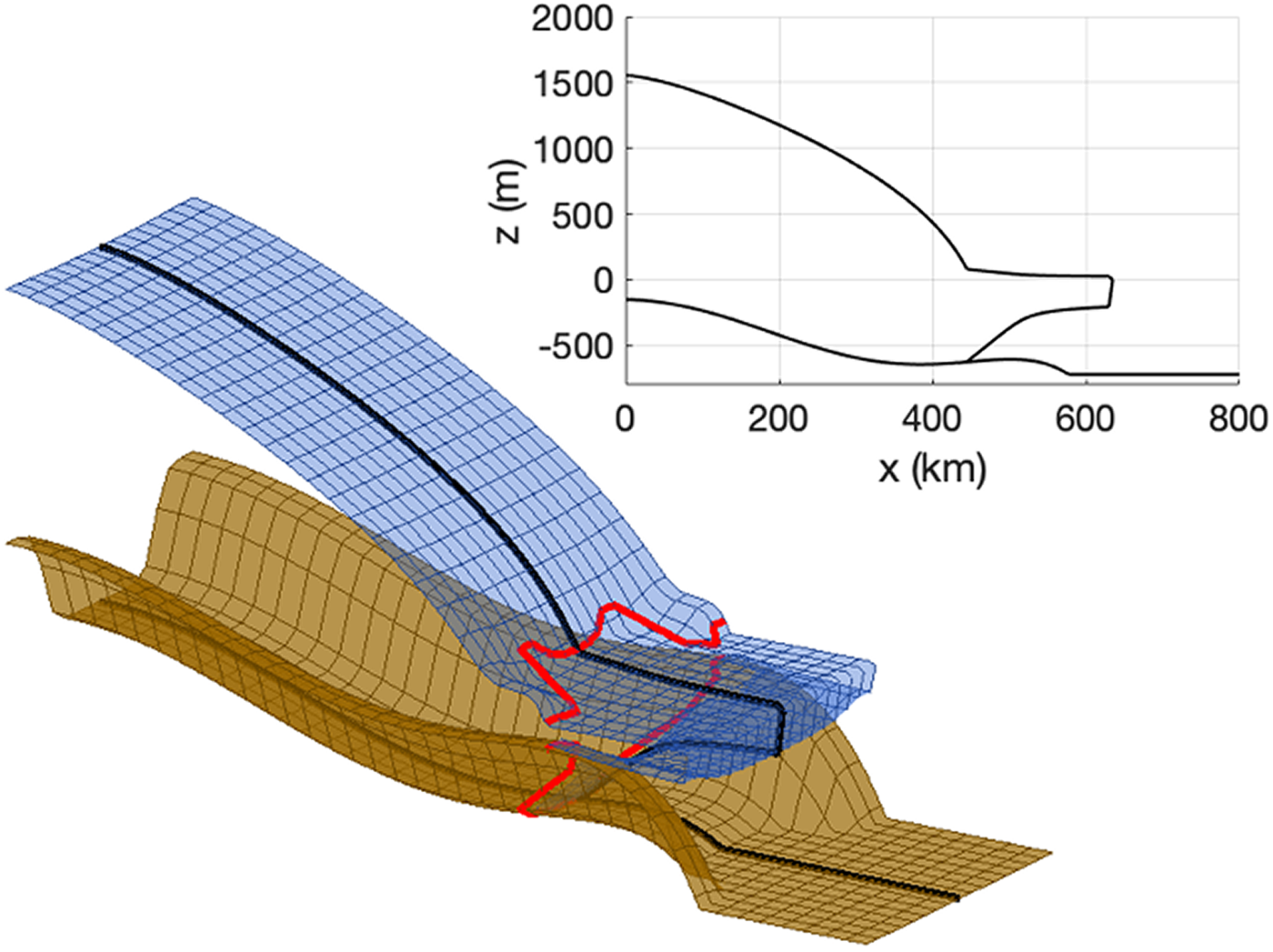
Asay-Davis and others (Reference Asay-Davis2016) proposed three interrelated marine ice-sheet/ocean model intercomparison projects: the Marine Ice-Sheet Model Intercomparison Project phase 3 (MISMIP+), the Ice-Shelf-Ocean Model Intercomparison Project phase 2 (ISOMIP+), and the Marine Ice-Sheet-Ocean Model Intercomparison Project (MISOMIP1). All three experiments concern the same idealised geometry, which represents an ice stream flowing into a constrained ice shelf. The grounding line has a stable position on a retrograde slope, which is made possible by the strong buttressing provided by the embayment. Underneath the shelf, the bathymetry forms a small sill that potentially prevents warm bottom water from flowing into the cavity. This idealised geometry is depicted in Figure 4.
The MISMIP+ idealised geometry. The grounding line and its projection on the ice surface are shown in red; a cross-section along y = 0 is shown in the top-right panel. z = 0 is equal to sea level, which is kept constant in time.
The three intercomparison experiments differ in their treatment of ice dynamics and ocean circulation: MISMIP+ only concerns ice dynamics, using a simple local melt parameterisation. ISOMIP+ only concerns ocean circulation, prescribing a fixed ice-sheet geometry (obtained from the spin-up phase of MISMIP+). MISOMIP1 concerns both ocean circulation and ice dynamics; time-dependent vertical temperature and salinity profiles are prescribed at the domain boundary, so that melt rates should be dynamically calculated using an ocean model.
3.1 MISMIP+
In order to verify that the new sliding laws have been implemented correctly, and also to produce the steady-state ice-sheet geometry required to initialise the MISOMIP1 simulations, we performed the experiments stipulated by the MISMIP+ protocol (Asay-Davis and others, Reference Asay-Davis2016). First, the ice sheet is spun up to a steady state, where the grounding-line position along the ice-stream centreline should be at x = 450 km. This can be achieved by tuning either the bed roughness, or the prescribed uniform ice flow factor; we chose the latter option. After this has been achieved, the MISMIP+ protocol describes five different experiments: a zero-forcing control run, and four different retreat-advance combinations, which are listed in Table 5. Note that in experiments Ice2rr and Ice2ra, ‘increased calving’ means that a uniform (very) high melt rate is applied to a large downstream part of the shelf, following the MISMIP+ protocol (Asay-Davis and others, Reference Asay-Davis2016).
The five experiments in the MISMIP+ protocol

We performed all five experiments with the Weertman, Tsai and Schoof sliding laws, as described by Asay-Davis and others (Reference Asay-Davis2016). All simulations were performed at resolutions of both 5 and 2 km, using all three of the sub-grid melt schemes (NMP, FCMP and PMP), and using both the DIVA and the hybrid SIA/SSA ice dynamics. These three sliding laws, two resolutions, three sub-grid melt schemes and two stress balances would result in an ensemble of 36 simulations per experiment. However, only 27 of these were performed, as the combination of the hybrid SIA/SSA stress balance with the high 2 km resolution was deemed to be too computationally expensive. For each individual combination of sliding law, resolution and stress balance, the ice flow factor was separately tuned to attain a stable grounding line at the desired position. The results of the five MISMIP+ experiments are shown in Figure 5, where they are compared to the model intercomparison results presented by Cornford and others (Reference Cornford2020) which used the same set-up. The results of the IMAU-ICE simulations generally lie within the range of the model ensemble presented by Cornford and others (Reference Cornford2020), towards the upper end of the ensemble. This suggests that IMAU-ICE is generally less sensitive to oceanic forcing than some other ice-sheet models.
Grounding-line position over time in the MISMIP+ experiments, compared to the model intercomparison results by Cornford and others (Reference Cornford2020). For IMAU-ICE, the ensemble mean is indicated by a solid line, and the range by the shaded areas. For Cornford and others (Reference Cornford2020), the ensemble mean is indicated by a dotted line, and the range by dashed lines. (a) ice0, ice1rr and ice1ra. (b) ice0, ice2rr and ice2ra. Mind the differing y-axis scales.

In Figure 6 we show the results of the ice1rr experiment, separated by the choice of resolution, sliding law, stress balance approximation and sub-grid melt scheme. These results show that the choice of sliding law and of stress balance has a negligible effect on the results. This conclusion differs from that of Cornford and others (Reference Cornford2020), who report a difference in grounding-line retreat rates of ~25% between the Weertman sliding on the one hand, and the Tsai/Schoof sliding on the other. However, their findings are based on results from a large number of different ice-sheet models (their Fig. 7b), some of which were run with both sliding laws, while others were only run with either one. Their ensemble of Weertman-sliding models is therefore not the same as their ensemble of Coulomb-sliding models, so that the difference might also be caused by other inter-model differences. Cornford and others (Reference Cornford2020) also suggest that the spread might be related to differences in the initial grounding-line position, which are substantially smaller in our results.
Grounding-line position over time in the MISMIP+ ice1rr experiment, separated by the choice of (a) resolution, (b) sliding law, (c) stress balance approximation and (d) sub-grid melt scheme. The default choices are 2 km resolution, Schoof2005, DIVA and FCMP. This means that e.g. the blue line in panel A has all of these, except for the resolution, which is 5 km.

First column: thermal forcing at the shelf base, for the WARM (upper row) and COLD (lower row) ocean profiles in the MISMIP+ steady-state geometry. Other columns: sub-shelf melt rates produced by the six different melt parameterisations. The 300 m shelf draft contour and the grounding line are indicated by the dashed and solid black lines, respectively.

The combination of resolution and sub-grid melt scheme can significantly affect the results (Fig. 6, panel D). Both the NMP and PMP schemes yield strongly resolution-dependent results; the FCMP scheme yields nearly identical results at 5 and 2 km. The results from the NMP and PMP schemes converge to those of the FCMP scheme with increasing resolution, indicating that the FCMP scheme is the most reliable.
3.2 MISOMIP1
Although MISOMIP1 was originally meant to be an intercomparison of coupled ice-sheet/ocean models, it is also an ideal test case for the different sub-shelf melt parameterisations that are newly included in IMAU-ICE. The experimental protocol prescribes vertical temperature and salinity profiles at the domain boundary; these are meant to serve as boundary conditions for the ocean model, but they can also be directly used to force the different melt parameterisations. Two temperature profiles are provided: COLD describes a uniform ocean temperature of −1.9 $^\circ$ C, where WARM has a value of −1.9 $^\circ$
 C at the surface, which increases linearly to 1 $^\circ$
 C at a depth of 720 m (the deepest part of the subglacial bed). MISOMIP1 assumes that the ocean model has been tuned following the ISOMIP+ protocol: the average melt rate over the part of the shelf with a draft of more than 300 m must be 30 ± 2 m a−1 in the WARM scenario (Asay-Davis and others, Reference Asay-Davis2016). We achieve this by tuning γ T separately for each of the six melt models (linear, quadratic, M+, plume, PICO and PICOP), which is done by performing a simple parameter sweep through a range around the values reported by Favier and others (Reference Favier2019); values are listed in Table 6. All other tuneable parameters (e.g. the overturning strength C in PICO; Reese and others, Reference Reese, Albrecht, Mengel, Asay-Davis and Winkelmann2018, their Table 1) are the same as in their original publications. The resulting sub-shelf melt fields for both ocean profiles are shown in Figure 7. The average melt rates of the part of the shelf with a draft of more than 300 m are within 0.1 m a−1 for all six parameterisations. We note that Favier and others (Reference Favier2019) investigated different choices of tuning metric (e.g. changing the 300 m depth threshold) and consequently found different optimal parameter values (their Fig. 9 and F1).
Tuning parameters (γ T, in m s−1) for the different sub-shelf melt parameterizations resulting from the MISOMIP protocol, and the alternative values for the Antarctic experiments described in Section 4.2, based on Burgard and others (Reference Burgard, Jourdain, Reese, Jenkins and Mathiot2022) [B22] and Jourdain and others (Reference Jourdain2020) [J20]

For the PICO and PICOP simulations using [B22], additionally the overturning strength is changed from default 1.0 × 10⁻⁶ to 5.1 × 10⁻⁶ (50 km) and 0.12 × 10⁻⁶ (offshore) m6 s−1 kg−1
The experiments in MISOMIP1 follow the same structure as those in MISMIP+: a single control run, and four different retreat/advance-combinations. In this case, retreat (advance) is enforced by setting the ocean forcing to the WARM (COLD) profile. The control run maintains the COLD profile throughout the simulation. Note that this differs from MISMIP+, where the control run prescribes zero melt. Since the MISOMIP1 simulations are initialised with the steady-state ice-sheet resulting from MISMIP+, this means that a small drift is to be expected in the MISOMIP1 control runs. Another minor difference with respect to MISMIP+ is the way calving is prescribed in the Ice2 experiments. In MISOMIP1, both IceOcean1 and IceOcean2 still have a fixed ice front at x = 640 km, but additionally a threshold-thickness calving law is included in the Ice2 experiments (with a threshold thickness of 100 m); see Asay-Davis and others (Reference Asay-Davis2016) for details.
We performed all five experiments with three different sliding laws (Weertman, Tsai, Schoof), at different two resolutions (5 and 2 km), and with all six sub-shelf melt parameterisations, for a total of 36 ensemble members per experiment. All simulations used the DIVA stress balance and the FCMP sub-grid melt scheme. The results of these experiments are shown in Figure 8.
Grounding-line position over time in the MISOMIP1 experiments. (a) IceOcean1 experiments (fixed ice front). (b) IceOcean2 experiments (fixed ice front + threshold-thickness calving). (c) IceOcean1 experiments relative to the IceOcean0 control. (d) IceOcean2 experiments relative to the IceOcean0 control. Bars on the right-hand side of the panels indicate range of grounding-line positions per melt model at the end of each experiment (with 0 = cold ocean, rr = warm ocean and ra = 100 years warm followed by 100 years cold). Each shaded area represents the ensemble of six simulations for a single melt parameterisation, e.g. the green shaded area indicates the range of values resulting from the three sliding laws and two resolutions, when using the PICO melt parameterisation.

The figure clearly shows that differences in grounding-line position (indicated by the lines) at the end of the experiment among different melt models are generally larger than the differences (indicated by the shading) resulting from the choice of sliding law or resolution for any given melt model. This conclusion holds both for the absolute retreat curves shown in panels A and B, and for the retreat curves relative to the small drift in the IceOcean0 control experiments, shown in panels C and D.
4. Realistic Antarctic geometry experiments
4.1 ABUMIP ABUM simulations
Using a realistic present-day Antarctic bedrock topography and initial ice-sheet conditions from the Bedmachine dataset (Morlighem and others, Reference Morlighem2020), we conduct the Antarctic Buttressing Model Intercomparison Project (ABUMIP) ABUM experiment (Sun and others, Reference Sun2020). This entails a 500-year simulation with excessive sub-shelf melt rates of 400 m a−1 imposed to effectively remove all ice shelves. The experiment serves to quantify the effect of complete ice shelf removal on the upstream grounded ice, and hence on sea level. Here we test how the model results are affected by changes in resolution, basal sliding and sub-grid melt scheme.
We perform the experiment repeatedly using varying settings for the sliding law, the enhancement factor of grounded ice flow (f enh,gr), the sub-grid melting scheme and the resolution. At 32 km resolution, we use all five implemented sliding laws and sub-grid melt schemes (FCMP, NMP and PMP). We use the default setting f enh,gr = 1, as well as f enh,gr = 5 for the tuneable flow enhancement factor, bracketing the range found in recent literature (e.g. De Boer and others, Reference de Boer2015). At 16 km resolution and 10 km resolution, we only conduct simulations using f enh,gr = 1, and FCMP. Using the Schoof sliding law, we additionally use NMP and PMP (f enh,gr = 1), and f enh,gr = 5 (FCMP) at 16 km resolution. The surface mass balance is obtained from present-day (1979–2014 average) RACMO2.3 regional climate model results (van Wessem and others, Reference van Wessem2014), remapped to the resolution of the ice-sheet model using OBLIMAP (Reerink and others, Reference Reerink, van de Berg and van de Wal2016). A spin-up for the experiment is performed separately at all resolutions, and consists of two phases. First, a 100-year run with steady-state present-day climate to smooth the initial settings, during which no basal melt is applied. This is followed by a 240 ka thermodynamical simulation of two glacial cycles without ice dynamics (i.e. with unchanging ice geometry) to initialize the ice temperature. After the spin-up, the ice-sheet interior is not in equilibrium with the forcing. Hence, the ice sheet will adapt to the surface mass balance when the runs are initiated, in some cases even leading to positive ice volume changes after ice shelf removal. Achieving a (quasi) stable state after initialisation matching the observed geometry is problematic because of poorly constrained ocean conditions in the cavities, as well as the (over-)simplifications underlying the sub-shelf melt parameterisations. Such a state would require the use of an inversion, either for ocean temperatures or directly for melt rates as is done e.g. in Berends and others (Reference Berends, Goelzer, Reerink, Stap and van de Wal2022). In future work, we will design a more sophisticated spin-up including spatially variable basal roughness, which will then also be used for more realistic projections of the Antarctic ice sheet. Our aim here, however, is more exploratory in nature. We focus on assessing the relative differences caused by the varying parameters, for which we deem it appropriate to use the current spin-up, which is the same for every simulation. This means the absolute sea-level responses should not be taken at face value, but rather relative to each other. The alternative choice of performing a spin-up separately for every individual sub-shelf melt parameterization would imply that the differences between them can no longer be assessed by their effect on the sea-level response, but rather on the resulting estimated ocean temperatures. While such an investigation would be interesting, we deem it to be beyond the scope of this project.
Depending on the settings, we obtain widely differing results. The change in ice volume after 500 years ranges from +1.4 m sea-level equivalent (m.s.l.e.; Weertman sliding, NMP, f enh,gr = 1, and 32 km resolution; Fig. 9a) to −17.3 m.s.l.e. (Schoof sliding, PMP, f enh,gr = 5, and 32 km resolution; Fig. 9b), a 18.7 m.s.l.e. difference. In the former simulation, ice thickness is reduced in the interior of the East Antarctic ice sheet, but builds up everywhere along the fringes, except along the Ross and Filchner-Ronne ice shelves, due to very high friction. In the most responsive simulation, the West Antarctic ice sheet collapses completely. In addition, all areas of the East Antarctic ice sheet currently grounded below sea level lose vast amounts of ice, partly caused by the fact that, following the ABUMIP protocol, glacial isostatic adjustment is neglected and is therefore not stabilizing the mass loss. In the following, we explore the influence of the parameters we vary in more detail.
Ice thickness at the end of the 500-year ABUMIP ABUM experiment, using (a) Weertman sliding, f enh,gr = 1, NMP, and (b) Schoof sliding, f enh,gr = 5, PMP, both at 32 km resolution. Cyan areas indicate remnants of ice shelves. These are respectively the least and most responsive simulations of the ensemble.

In Figure 10a, we show the time-varying ice volume above flotation (in m.s.l.e.) for the simulations at 32 km resolution using f enh,gr = 1 and FCMP, using the five different sliding laws. Using Weertman sliding leads to a very weak response to ice shelf removal, while the Coulomb, Tsai and Schoof sliding laws lead to much stronger responses that are virtually identical to each other. This is largely due to the uniform basal roughness value of β 2 = 1 × 10⁶ Pa m−1/3 year1/3 that we apply, which results in high basal friction and hence low basal sliding velocities. In the Tsai and Schoof sliding laws, this β 2 value causes the ‘Coulomb part’ to dominate the sliding term. If we use β 2 = 1 × 10⁴ Pa m−1/3 year1/3 we obtain a much larger loss of grounded ice in all three cases (Fig. 10a, dashed lines); however, this results in a general overestimation of the ice surface velocities in the interior (not shown). The Budd-type sliding law leads to less sea-level rise than Coulomb sliding, by using the default constant till friction angle φ = 150 (Fig. 10a) as well as by using a lower value φ = 50 (not shown).
(a) Evolution over time of ice volume above flotation in the ABUMIP ABUM experiment using (a) different sliding laws and basal roughness (32 km resolution, FCMP, f enh,gr = 1) (solid green, black and blue lines overlap, only blue is visible), (b) different flow enhancement factors (32 km resolution, FCMP), (c) different sub-grid melt schemes (32 km resolution, f enh,gr = 1), and (d) different resolutions (f enh,gr = 1).

We additionally perform control simulations including ice shelves, i.e. the ABUMIP control experiment (ABUC). The response of grounded ice volume to present-day ocean forcing is very strongly dependent on the choice of sub-shelf melt parametrisation, which we address in Section 4.2. To compare ABUMIP simulations, here we choose a neutral method of keeping the ice shelf geometry fixed. This is implemented as basal melt cancelling mass change through ice flow and the surface mass balance, similar to inverting basal melt to obtain observed ice shelf heights (Bernales and others, Reference Bernales, Rogozhina and Thomas2017). While this approach possibly overestimates the stability of the grounded ice, it avoids masking the sensitivity to the choice of sliding law by choosing a melt parameterisation that over(under)estimates melt, leading to thinning (thickening) shelves and accelerated (stagnated) sliding. These ABUC simulations show a significant but small drift: ice volume changes are smaller than 1 m.s.l.e. over the 500-year integration period when the default basal roughness values are used (Fig. S1a, solid lines). Hence, ABUM minus ABUC yields qualitatively very similar results as ABUM (Fig. S1b, solid lines). However, this does not hold for the simulations using lower basal roughness values, in which ABUC already yields ~4 m ice volume loss (Fig. S1a, dashed lines). Consequently, ABUM minus ABUC shows considerably smaller differences in ice volume loss (Fig. S1b, dashed lines). This means that, for these settings, the ice volume loss due to removing ice shelves per se is smaller than the ABUM simulation suggests. The ABUM results themselves nevertheless indicate how the grounded ice behaves in absence of ice shelves for the various settings we have explored.
Faster flowing grounded ice, caused by an increase of the flow enhancement factor, leads to a larger ice volume loss in all investigated cases. This is shown for the combinations of Schoof and Weertman sliding with FCMP, at 32 km resolution in Figs 10b and S1c, d). The difference after 500 years amounts to 3.5 m.s.l.e. averaged over all sliding laws and sub-grid schemes at 32 km resolution, ranging from 1.5 m.s.l.e. for the Weertman sliding law, to 4.3 m.s.l.e. for the Schoof sliding law.
Like in the simulations using idealized geometry, the PMP leads to a larger, while the NMP leads to a smaller response than the FCMP sub-grid melt scheme. This is shown for the combinations of Schoof and Weertman sliding laws with f enh,gr = 1, at 32 km resolution in Figure 10c. The Weertman simulations yield a difference of 4.7 m.s.l.e. between PMP and FCMP, and 2.2 m.s.l.e. between FCMP and NMP. For the Schoof simulations, these differences amount to 9.7 and 1.8 m.s.l.e. respectively.
Using the Schoof sliding law, FCMP and f enh,gr = 1, the grounded ice mass change is reduced at higher resolution, but the effect is relatively small (~0.6 m.s.l.e.; Figs 10d and S1e, solid lines). Using a higher flow enhancement factor (f enh,gr = 5), as well as using different sliding laws, we obtain similar differences between the responses at 16 and 32 km resolution (not shown). Most noteworthy, however, the differences caused by the sub-grid melt schemes converge at higher resolution, as the NMP yields a little bit more, while the PMP yields considerably less ice loss (Figs 10d and S1f, dashed and dotted lines). Similar as in the idealized experiments, FCMP also yields a little bit less ice loss at higher resolution (Fig. 10d, solid lines), hence it is likely that at hypothetical infinite resolution the schemes converge towards somewhere in the middle between NMP and FCMP.
4.2 Ocean-forced simulations
To test the sensitivity of our model to ocean forcing, we perform experiments using all six implemented sub-shelf melt parameterisations (Section 2.3), forced by present-day WOA temperature and salinity data (Locarnini and others, Reference Locarnini2019; Zweng and others, Reference Zweng2019). We apply the so-called objectively analysed mean fields at 1° resolution, extrapolated underneath the ice shelves at 5 km resolution as described in Section 2.4. We refrain from using temperature corrections to obtain present-day melt rates in individual sectors close to observations (Jourdain and others, Reference Jourdain2020). The spin-up and atmospheric forcing are the same as in the ABUMIP ABUM experiment (Section 4.1). We deploy the Schoof sliding law with FCMP sub-grid melt and set the flow enhancement factors of grounded and floating ice to unity. Floating ice thinner than 200 m is calved off. In lieu of accurate projections of the Antarctic ice sheet, here we aim to make an independent assessment of the different sub-shelf melt parameterisations in a realistic present-day Antarctic topography. To this end, we prefer the tuning approach following the MISOMIP protocol, above tuning towards a realistic present-day state, because in the idealized MISOMIP1 set-up, there are no unknown processes or uncertain observations to complicate matters. This is therefore the purest comparison between the sub-shelf melt parameterisations. For this reason, we set the values for the settings in the sub-shelf melt parameterisations to those calibrated in the MISOMIP1 experiment (Section 3.2, Table 6). This means that, similar to our ABUMIP experiments, the sea-level responses for the different sub-shelf melt parameterisations should again only be regarded relative to each other and not in absolute sense.
The sub-shelf melt parameterisations yield widely differing results for the WOA-forced experiments. At 32 km resolution, the drift in ice volume above flotation ranges from −0.2 m.s.l.e. (PICOP) to −1.9 (M+) after 100 years of integration (Fig. 11a). This drift becomes less negative at 16 km resolution, ranging from +0.8 to −1.3 m.s.l.e. (Fig. 11b). The large ice volume loss in the simulations using linear and M+ sub-shelf melt is caused by excessive sub-shelf melt rates for all floating ice (Fig. 12). The quadratic sub-shelf parameterisation yields results closer to observations using this parameter tuning, with strong melting in the Bellinghausen and Amundsen Sea sectors (Fig. 12, top row) and along the coasts of Wilkes Land and Dronning Maud Land (not shown). More modest melting occurs in the Ross and Filchner-Ronne embayments (Fig. 12, middle rows), increasing towards the grounding line. Sub-shelf freezing does not occur anywhere. PICO yields similar realistic results as the quadratic sub-shelf parameterisation but does calculate sub-shelf freezing on large parts of the Ross and Ronne ice shelves. For the Ross ice shelf, the requirement that the sub-shelf melt rate is positive in the first ocean box is not met using these parameter settings. More extreme sub-shelf melt rates are obtained using the plume parameterisation, both in positive sense (i.e., stronger melt) in the Bellinghausen and Amundsen Sea sectors and along the coasts of Wilkes Land and Dronning Maud Land, and in the negative sense (i.e. stronger freezing) in the Ross and Filchner-Ronne embayments. Using PICOP, sub-shelf freezing occurs almost everywhere.
(a) Evolution over time of ice volume above flotation (af) in the experiments using ocean forcing from World Ocean Atlas (WOA) data at 32 km resolution and (b) at 16 km resolution, with different sub-shelf melt parameterisations using parameters tuned following the MISOMIP protocol, and with fixed ice-shelf geometry for reference (REF; first 100 years of the ABUMIP ABUC experiment).

(a) Evolution over time of ice volume above flotation (af) in the experiments using ocean forcing from World Ocean Atlas (WOA) data at 32 km resolution and (b) at 16 km resolution, with quadratic and M+ sub-shelf melt parameterisations using MISOMIP tuning, and using parameter settings obtained from Jourdain and others (Reference Jourdain2020) [J20]. The shading envelopes the range yielded by the 5th to the 95th percentile values of the MeanAnt tuning. The dotted and dashed lines represent the median values of the MeanAnt and PIGL tunings respectively. (c–d) Same for the PICO and PICOP sub-shelf melt parameterisations using MISOMIP tuning, and using parameter settings obtained from Burgard and others (Reference Burgard, Jourdain, Reese, Jenkins and Mathiot2022) [B22]. The parameter settings for these experiments are listed in Table 6.

The importance of the parameter settings is demonstrated by additional simulations, in which we use settings obtained from the recent studies of Jourdain and others (Reference Jourdain2020) for the quadratic and M+ sub-shelf melt parameterisations and Burgard and others (Reference Burgard, Jourdain, Reese, Jenkins and Mathiot2022) for PICO and PICOP (Table 6). Note that we refrain from using their plume parameterisation values, as they tune different parameters than we do. Jourdain and others (Reference Jourdain2020) used the MeanAnt tuning to obtain a realistic instantaneous basal mass balance with WOA ocean data underneath the ice shelves integrated over the whole Antarctic ice sheet. Using these values (5th percentile, median and 95th percentile) leads to a generally smaller ice loss than our standard parameter settings, both at 32 and 16 km resolution (Figs 12a, b). The larger values of the PIGL tuning, aimed to specifically obtain realistic melt rates underneath the Pine Island ice shelf, lead to much stronger ice volume loss. Burgard and others (Reference Burgard, Jourdain, Reese, Jenkins and Mathiot2022) tuned the parameters (γ T as well as the overturning strength) of PICO and PICOP to obtain the best possible match to the sub-shelf melt rates around Antarctica produced by the NEMO ocean model, using offshore hydrographic input fields and profiles averaged over a domain of 50 km on the continental domain in front of the ice shelf. These values lead to less ice volume loss than our standard tuning for PICO, while for PICOP the 50 km tuning leads to more, and the offshore tuning to comparable ice volume loss (Figs 12c, d).
These alternatively calibrated results testify to the fact that a large range of outcomes can be obtained with each individual sub-shelf melt parameterisation depending on the choice of parameter settings. In all cases, this could potentially include an Antarctic ice sheet that remains relatively stable in size after initialisation under present-day forcing. Therefore, on the basis of our results no single parameterisation can be rejected. However, our simulations using MISOMIP tuning do demonstrate that tuning towards present-day observations obscures the effect of the different ways in which all these parameterisations deal with the effects of (changing) topography and ocean circulation.
To gain further understanding of the sensitivity of the different sub-shelf melt parameterisations to ocean forcing, we additionally perform ice-sheet experiments using ocean forcing from simulations by the Community Earth System Model (CESM; van Westen and Dijkstra, Reference van Westen and Dijkstra2021). CESM was run for 100 years (2000–2100 AD) using constant present-day forcing (control) and using a CO2 concentration increasing by 1% per year. The simulations were performed using a low horizontal oceanic resolution (LR) of 1° × 1° and a high resolution (HR) of 0.1° × 0.1°. Here, we use the yearly average 3D ocean temperature and salinity fields at present day (repeated year 2100 AD), extrapolated underneath the ice shelves (which are not represented in CESM) as before, to force our simulations over 100 years. Again, we set the values for the settings in the sub-shelf melt parameterisations to those calibrated in the MISOMIP1 experiment (Table 6).
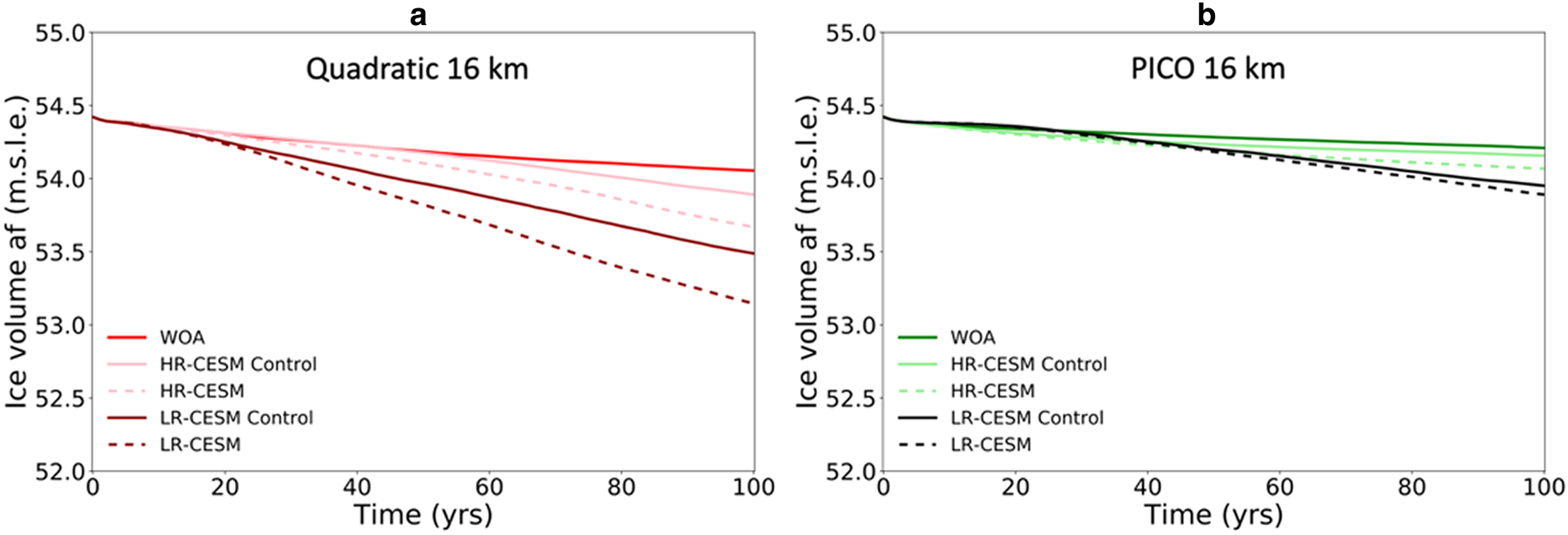
In Figure 14, we show the ice volume above flotation over time from the simulations at 16 km resolution using the sub-shelf melt parameterisations that gave the most realistic sub-shelf melt rate patterns when forced by the present-day WOA data (using the MISOMIP1 parameter tuning; Fig. 13), being quadratic melt and PICO. In both cases, the drift in the HR-CESM control run is smaller than in the LR-CESM control run, and closer to the drift in the WOA-forced simulations. This is due to the temperatures below the ice shelves, for instance in the Amundsen Sea, Filchner-Ronne and Amery embayments, which are closer to those of WOA for the HR-CESM than for the LR-CESM forcing, causing an also smaller difference in the sub-shelf melt rates (Figs S2 and S3). The temperature difference between the CESM runs is caused by HR-CESM explicitly resolving ocean eddies and more accurately capturing boundary currents at high resolution, leading to a more realistic Southern Ocean temperature distribution and volume transport (van Westen and Dijkstra, Reference van Westen and Dijkstra2021; their Fig. S1). Both the HR-CESM and LR-CESM results show an abrupt East–West temperature gradient in the Ross Embayment. This is likely an artefact due to the extrapolation of too warm temperatures at the West side of the shelf edge onto the shelf. This consequently leads to a strong gradient in sub-shelf melt rates for the quadratic parameterisation (Figs S2 and S3). PICO, however, uses a basin average forcing temperature obtained from the open ocean temperature in front of the shelf (Reese and others, Reference Reese, Albrecht, Mengel, Asay-Davis and Winkelmann2018). Hence, it does not calculate such an East–West sub-shelf melt rate gradient. The difference in ice volume above flotation after 100 years between the LR-CESM and HR-CESM control simulations amounts to 0.40 m.s.l.e. using the quadratic sub-shelf melt parameterisation, while PISM yields a 0.21 m.s.l.e. difference. Using quadratic melt, the differences between the perturbed and control CESM experiments are larger for LR-CESM (0.34 m.s.l.e.) than for HR-CESM (0.22 m.s.l.e.). Using PICO, however, the difference is slightly smaller for LR-CESM (0.06 m.s.l.e.) than for HR-CESM (0.09 m.s.l.e.). Like the WOA-forced simulations (Fig. 11), the CESM-forced simulations generally show larger ice volume loss in absolute sense at a lower resolution of the ice-sheet model (32 km; not shown). Overall, PICO appears less sensitive to changes in thermal forcing than the quadratic sub-shelf melt parameterisation. This is likely in part because it is less dependent on the cavity extrapolation of the ocean data (Section 2.4). In general, the differences caused by the thermal forcing (HR-CESM versus LR-CESM, and perturbed versus control simulations; Fig. 14) are smaller than the differences caused by the choice of sub-shelf melt parameterisation (Fig. 11).
Thermal forcing (leftmost column), and sub-shelf melt rates underneath the ice shelves at the start of the experiments at 16 km resolution using ocean forcing from World Ocean Atlas (WOA) data. Different sub-shelf melt parameterisations are applied, using parameter values as calibrated in the MISOMIP1 experiment (Table 6). For the forcing and each parameterisation, the rows show (top to bottom) the Amundsen Sea embayment, the Filchner–Ronne embayment, the Ross embayment and the Amery embayment.

(a) Evolution over time of ice volume above flotation in the experiments using ocean forcing from WOA, and low-resolution (LR) and high-resolution (HR) CESM (control and perturbed) simulations, with quadratic sub-shelf melt and (b) PICO, at 16 km resolution.
5. Discussion and conclusions
We have presented results from a large number of simulations of both idealized-geometry and realistic Antarctic topography, using different choices for the grid resolution, the sliding law, the stress balance approximation, the sub-grid melt scheme, the sub-shelf melt parameterisation and the ocean forcing data.
We find that, both in the idealised-geometry and in the realistic Antarctic geometry experiments, the FCMP sub-grid melt scheme results in the weakest dependency on grid resolution. The NMP and PMP schemes both show a strong dependence on resolution, resulting in strongly reduced (increased) retreat rates for the NMP (PMP) scheme; both converge towards the results of the FCMP scheme with increasing resolution. This agrees with the findings of Leguy and others (Reference Leguy, Lipscomb and Asay-Davis2021), who found that the FCMP and PMP scheme generally outperform the NMP scheme, but they found smaller differences between FCMP and PMP than we do. This difference might be partly caused by the fact that CISM uses a different discretization scheme than IMAU-ICE, defining velocities on the Arakawa B-grid instead of the C-grids. While earlier studies, such as Seroussi and Morlighem (Reference Seroussi and Morlighem2018) and Cornford and others (Reference Cornford2020), argue that no melt should be applied to any partly grounded gridcell, i.e. the NMP scheme, we agree with Leguy and others (Reference Leguy, Lipscomb and Asay-Davis2021) that the ultimate answer likely is more complex. The interplay between the sub-shelf melt rate (both in terms of magnitude, and of spatial distribution) and the geometry of the shelf cavity is intricate, and it seems likely that, until a more appropriate solution is formulated, the FCMP, PMP or NMP schemes might all be more appropriate in certain settings than in others. We believe that more structured schematic experiments like those performed by Leguy and others (Reference Leguy, Lipscomb and Asay-Davis2021), possibly investigating the relation with the numerical details of the ice-sheet model, are needed to find a comprehensive solution. The fact that the results converge towards the FCMP scheme for higher resolutions suggest that, in our model, the FCMP is the preferred option.
The choice of sliding law seems to have very little effect on the results in the idealised-geometry experiments. Cornford and others (Reference Cornford2020) find a stronger dependence, which might be caused by the different model ensembles used to investigate the different sliding laws, and the wider range in initial states. In contrast to the idealised-geometry experiments we do find a stronger dependence in our Antarctic experiments. This might be explained by the fact that, in the idealised-geometry experiments, for each individual combination of sliding law, stress balance and grid resolution, Glen's flow factor is tuned to achieve the same steady-state geometry. Since no such tuning is done for Antarctica (where the flow factor is calculated dynamically based on the evolving englacial temperature), differences are likely to be larger in those experiments. The fact that the grid resolution in the Antarctic experiments is considerably coarser likely also increases the differences between the simulations, as well as the fact that no separate Antarctic spin-ups are performed for each individual sliding law. In order to initialise a model with a steady-state ice sheet, it is therefore likely best to use a separate initialisation for each sliding law.
The different sub-shelf melt parameterisations result in very different retreat rates under warm ocean forcing, both in the idealised-geometry and in the realistic Antarctic geometry experiments. Although all parameterisations were tuned following the same protocol, which is loosely based on high-resolution ocean model results in an idealised-geometry set-up (Asay-Davis and others, Reference Asay-Davis2016), they all have a different way to factor in changes in the geometry of the shelf cavity. This largely explains the different dynamical response of the ice sheet in the idealised-geometry setting. In the Antarctic setting, there is likely an additional contribution from the fact that we tuned for identical results in the idealised rather than the Antarctic geometry. This calls for individually tuning the different parameterisations towards present-day melt rates for the purpose of making realistic projections. We note however that such an approach should be seen as a first step towards reliable sea-level projections, not a guarantee, as the spread and uncertainty in the observed melt rates is large enough to cause significant differences in model results, depending on the choice of tuning metric. We also note that tuning melt sensitivity parameters rather than ocean temperatures (as is now done in the ISMIP protocol) can additionally affect the sensitivity to future ocean warming, making it difficult to constrain the uncertainty in this regard.
The range of Antarctic mass losses resulting from the choice of sub-shelf melt parameterisation we obtain in our simulations is as large as that of the choice of sliding law and ice viscosity, and significantly larger than the range resulting from the resolution and forcing scenario of the model providing the ocean forcing. This strong impact on the dynamical response indicates that, although it is important to have good constraints on the state of the ocean in future warming scenarios, the relation between that ocean state and the resulting sub-shelf melt rate is at least as, if not more, important. We have not sampled the entire range of possible modelled ocean conditions. By including versions of CESM with a different resolution, both with constant present-day conditions and under strong warming, as well as present-day observations from the WOA, we have gained a good first estimate of the uncertainty in the ocean forcing. Based on this (small) sample of different ocean models, we conclude that the uncertainty arising from the ocean forcing itself is likely smaller than that arising from the choice of sub-shelf melt parameterisation.
The experiments presented here are of an exploratory nature, and should only be interpreted as a sensitivity analysis. They are not to be viewed as actual projections of future ice-sheet retreat; for such experiments, a more elaborate initialisation procedure and surface mass-balance forcing is required. Similarly, whereas other studies, such as Favier and others (Reference Favier2019) and Burgard and others (Reference Burgard, Jourdain, Reese, Jenkins and Mathiot2022), compare the melt rates of the different sub-shelf melt parameterisations to observed or ocean-modelled melt rates, our results should not be viewed through that particular lens. Rather, we show that, even when the different parameterisations are tuned to yield comparable basin-averaged melt rates in a controlled setting, they still yield widely different ice-sheet retreat rates when applied in a ‘warm ocean’ scenario, both in idealised and realistic settings. However, disregarding the differences in modelled melt rates, we do note that not all parameterisations are equally practical in terms of implementation. The more complicated plume, PICO and PICOP parameterisations, due to their inherently 1-D nature (and the rather convoluted and/or ad hoc solutions to extend them to two dimensions), are significantly more difficult to implement in a dynamic ice-sheet model, than the (semi-)local linear, quadratic and M+ parameterisations. Based on our results, in addition to those of Favier and others (Reference Favier2019) and Burgard and others (Reference Burgard, Jourdain, Reese, Jenkins and Mathiot2022), we do not believe there yet exists a single melt parameterisation that clearly performs better than any of the others in all settings. For our (palaeo-)ice-sheet simulations that require a parameterisation robust enough to handle large changes in ice-sheet geometry, we therefore prefer the more readily applicable local parameterisations.
Our findings highlight several avenues where future research is needed. The question whether any simple melt parameterisation like the ones tested here can provide reliable results in any geometry and ocean regime, or if flow-resolving ocean models are the only way forward, remains open. The question of how to deal with unknown ocean conditions in the cavity, in the context of model calibration and initialisation, likewise is one that requires further study. Several modelling groups are now exploring the possibility of using inversion methods to determine sub-shelf ocean conditions, similar to approaches that are already used for basal friction (e.g. Bernales and others, Reference Bernales, Rogozhina and Thomas2017). Future work should therefore include investigating the sensitivity to the choice of melt parameterisation and/or ocean forcing, when these choices are also reflected in the model initialisation. The interpretation of a modelled sea-level change (or lack thereof) as ‘drift’ in such a setting is something that needs to be carefully considered. Any inversion method (or any other form of parameter tuning) will intrinsically generate compensating errors for imperfect model parameters (e.g. Berends and others, Reference Berends, van de Wal, van den Akker and Lipscomb2023). This implies that the presence of drift does not necessarily mean that the applied melt parameterisation (or the initialisation procedure, or the sliding law, or the friction field, etc.) is wrong, just as the absence of drift does not mean that any or all of these model components are correct.
Supplementary material
The supplementary material for this article can be found at https://doi.org/10.1017/jog.2023.33
Acknowledgements
We thank René van Westen for providing the CESM results used as ocean forcing for some of our experiments, and for commenting on an earlier draft of this manuscript. We also thank the editor Frank Pattyn and two anonymous reviewers for their helpful comments on the manuscript.
Author contributions
C. J. B. wrote the code for the new sliding laws and sub-shelf melt parameterisations. C. J. B. performed the schematic experiments, L. B. S. performed the Antarctic experiments. C. J. B. and L. B. S. drafted the manuscript; all authors contributed to the final version.
Financial support
This publication was supported by PROTECT. This project has received funding from the European Union's Horizon 2020 research and innovation programme under grant agreement no. 869304 (PROTECT; [article number will be assigned upon acceptance for publication!]). The use of supercomputer facilities was sponsored by NWO Exact and Natural Sciences. Model runs were performed on the Dutch National Supercomputer Snellius. We would like to acknowledge SurfSARA Computing and Networking Services for their support. L.B. Stap is funded by the Dutch Research Council (NWO), through VENI grant VI.Veni.202.031.
Conflict of interest
None.
Code and data availability
The source code of IMAU-ICE is maintained on Github at https://github.com/IMAU-paleo/IMAU-ICE.


 Open access