


Introduction
Iceberg calving is an important mechanism of mass loss for the Antarctic and Greenland ice sheets and many glaciers around the world (Reference Jacobs, Hellmer, Doake, Jenkins and FrolichJacobs and others, 1992; Reference Hagen, Melvold, Pinglot and DowdeswellHagen and others, 2003;Reference Rignot and KanagaratnamRignot and Kanagaratnam, 2006). Observations of recent calving retreats and coincident flow acceleration at glaciers in Greenland and Antarctica (Reference De Angelis and SkvarcaDe Angelis and Skvarca, 2003;Reference Joughin, Abdalati and FahnestockJoughin and others, 2004;Reference Rignot, Casassa, Gogineni, Krabill, Rivera and ThomasRignot and others, 2004;Reference Howat, Joughin, Fahnestock, Smith and ScambosHowat and others, 2008) have served to illustrate the tight linkages between calving, glacier flow and terminus stability. Unfortunately, modeling of calving processes remains a major challenge, thus casting doubt on the ability of glacier and ice-sheet models to predict future sea-level variations.
A full calving model would describe the rapid (minutes to hours) evolution of glacier geometry and stress field that occurs as an ice block detaches from a glacier (e.g. Reference Pralong and FunkPralong and Funk, 2005). Reconciling the high temporal and spatial resolution necessary for such a model with the computational constraints of ice-sheet models is, however, an extremely difficult task. An alternative is to seek a parameterization of calving that is sufficiently general to be applicable to any calving margin, yet sufficiently simple to be implementable in ice-sheet models.
Previous efforts to parameterize calving include (1) relating the mean calving rate of grounded glaciers to water depth at the terminus (Reference Brown, Meier and PostBrown and others, 1982), (2) continuously adjusting the terminus position so that the terminus thickness always equals or exceeds some value given by a calving criterion (Reference Van der VeenVan der Veen, 1996; Reference Vieli, Funk and BlatterVieli and others, 2001, Reference Vieli, Jania and Kolondra2002; Reference Benn, Hulton and MottramBenn and others, 2007a, Reference Benn, Warren and Mottramb) and (3) relating the mean calving rate of ice shelves to ice-shelf thickness, width and strain rate (Reference AlleyAlley and others, 2008). The model of Benn and others (2007a,b) is the only model that can clearly be applied to both floating and grounded termini. In their model, the terminus is located where crevasse depth equals terminus freeboard, with crevasse depth depending on longitudinal strain rates and ponding of water in crevasses.
Despite the advances made by Reference Benn, Hulton and MottramBenn and others (2007a, Reference Benn, Warren and Mottramb), their crevasse-depth calving criterion cannot explain all calving variability. As an example, consider the terminus dynamics of Jakobshavn Isbræ, a rapidly flowing outlet glacier in Greenland. Currently, calving ceases during winter and the terminus advances ˜5 km. Calving typically resumes vigorously in March or April, and within a few weeks the terminus can retreat 3–4 km. The terminus continues retreating, albeit at a slower rate, throughout the summer (Reference Amundson, Truffer, Luthi, Fahnestock, West and MotykaAmundson and others, 2008). The onset of calving in spring precedes significant surface melting and summer flow acceleration, which occurs primarily in response to terminus retreat (Reference JoughinJoughin and others, 2008c); the spring retreat is not attributable to changes in strain rates or surface melting and therefore cannot be explained by the crevasse- depth calving criterion.
Parameterization of calving is confounded by the wide variety of calving phenomena, including the sub-hourly detachment of small ice blocks from grounded, temperate glaciers (Reference O’Neel, Echelmeyer and MotykaO’Neel and others, 2003, Reference O’Neel, Marshall, McNamara and Pfeffer2007), the roughly decadal calving of giant tabular icebergs (with horizontal dimensions of 10–100 km) from floating ice shelves (Reference Lazzara, Jezek, Scambos, MacAyeal and van der VeenLazzara and others, 1999) and the catastrophic collapse of thin ice shelves within a matter of days to weeks (Reference Rott, Skvarca and NaglerRott and others, 1996;Reference Scambos, Hulbe, Fahnestock and BohlanderScambos and others, 2000;Reference Braun and HumbertBraun and Humbert, 2009; Reference Braun and HumbertBraun and others, 2009). Although the aim of calving models is not to describe all calving events, the variations in size and frequency of calving events provide information about the processes controlling calving. Previous efforts to parameterize calving do not take these variations into account. Herein, we develop a framework for calving models that can account for the wide range of calving processes. The framework is based on the simple idea that terminus thickness is larger after a calving event than at the event onset, and that pre- and post-calving terminus thicknesses are given by two separate but related functions. The functions are left unspecified, and therefore new or existing calving models can be easily incorporated into the framework. We do, however, investigate the relationship between the functions by considering the wide spectrum of observed calving styles. In particular, the calving framework allows for a simple parameterization of the highly nonlinear, chain-reaction type processes that can cause large portions of an ice shelf to disintegrate in a matter of days (Reference MacAyeal, Okal, Aster and BassisMacAyeal and others, 2009).
2. Proposed Calving Framework
We propose a framework for calving models in which calving events are triggered when the terminus thickness decreases to some critical value, H 0. Once a calving event is initiated, the terminus rapidly retreats to the location where the terminus thickness equals some second critical value, H 1. H 0 and H 1 are unknown functions. As we show below, the ratio H 0/H1 strongly influences the size of and time period between calving events.
The proposed framework is essentially an extension to previously proposed, thickness-based calving criteria. For example, the Van der Veen/Vieli and Benn calving models amount to a specification of H 0 (in terms of terminus geometry in the former and crevasse depth in the latter) and the assumption that H 1 ≈ H 0. Our simple modification to these thickness-based calving criteria provides the flexibility necessary to fully characterize the wide variety of calving phenomena.
The framework is presented in several parts. We first use a steady-state analysis to investigate the primary controls on calving, and then show that our calving framework is consistent with the steady-state analysis (section 3). We then discuss possible physical interpretations of H 0 and H 1 and investigate the relationship between H 0 and H 1 by comparing our theoretical analysis with observations of calving dynamics (section 4). Finally, we demonstrate the framework’s versatility by using ad hoc functions for H 0 and H 1 to generate seasonal variations in terminus position (section 5).
3. Steady-State Analysis of Calving
The following analysis is developed in two horizontal dimensions to ease possible modification and implementation into glacier and ice-sheet models. In two dimensions, the change in terminus position with time for a calving glacier is given by
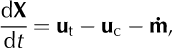
where X is terminus position, t is time, and u
t, u
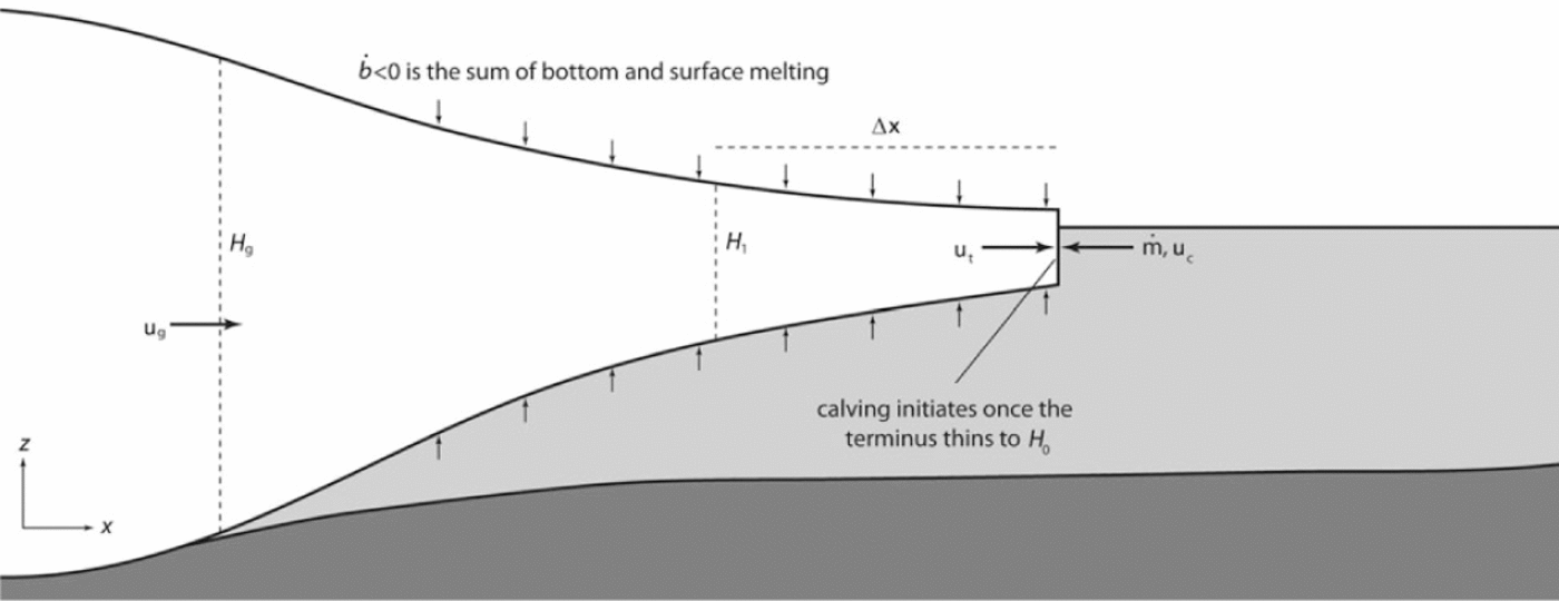
c and  are the vertically averaged terminus velocity, calving rate and melt rate of the vertical face of the terminus (Reference Motyka, Hunter, Echelmeyer and ConnorMotyka and others, 2003), respectively (Fig. 1). Bold face is used to indicate two-dimensional horizontal vectors; whenever the horizontal axes are oriented along a flowline, these vector quantities are expressed as (non-bold) scalars. We use to refer to both terminus melting and calving associated with nonuniform melting of the terminus (as discussed by Reference Vieli, Jania and KolondraVieli and others, 2002; Reference Motyka, Hunter, Echelmeyer and ConnorMotyka and others, 2003; Reference RöhlRöhl, 2006; Reference Rignot, Koppes and VelicognaRignot and others, 2010).
Schematic diagram of a glacier terminus indicating many of the variables used in the present analysis.
Over annual timescales, terminus velocity and calving rate tend to scale with each other. As a result, the rate of change of the terminus position is almost always one to two orders of magnitude smaller than terminus velocity or calving rate (Reference Van der VeenVan der Veen, 1996). The observation that calving rate and terminus velocity are numbers of similar magnitude that almost exactly cancel indicates that they are not independent of each other. Here we use steady-state and near steady-state analyses to identify the primary variables controlling calving (and therefore also controlling terminus velocity). The results support our choice for a general calving framework (section 2).
3.1. Continuous calving
For a glacier that is in steady state, dX/dt = 0. The calving rate is therefore given by

Terminus velocity, u t, can be estimated through the mass continuity equation, which dictates that for a column of ice
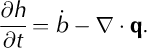
Here h is ice thickness,  is the combined surface and bottom mass-balance rate, =(∂/∂x, ∂/∂y) with x and y indicating map coordinates and q is horizontal ice flux. We let u equal the depth-averaged horizontal velocity, so that q = hū and Equation (3) becomes

we now note that

where u and v are horizontal velocities within the column and h b and h s are the bed and surface elevations. Note that h = h s–hb. Expanding Equation (5) using the product rule gives

The last two terms in Equation (6) are evaluated using the Leibniz rule, yielding

Where  and
and  are the depth-averaged normal strain rates and u
s and u
b are the horizontal surface and basal velocity vectors. Strain rates greater than zero are used to indicate extension. As a result, Δh<0 indicates that ice thickness decreases in the down-glacier direction, as is generally observed near a glacier terminus.
are the depth-averaged normal strain rates and u
s and u
b are the horizontal surface and basal velocity vectors. Strain rates greater than zero are used to indicate extension. As a result, Δh<0 indicates that ice thickness decreases in the down-glacier direction, as is generally observed near a glacier terminus.
Due to the incompressibility of ice,

Where  is the depth-averaged vertical normal strain rate. Inserting Equation (8) into Equation (7), and the result into Equation (4), gives

The depth-averaged velocity is some fraction, 0.8 ≤ β ≤ 1, of the surface velocity. β = 1 when the basal velocity equals the surface velocity, as is the case with ice shelves, whereas β = 0.8 in the shallow-ice approximation for an isothermal glacier that is not sliding over its bed. Both nonzero basal velocities and/or concentrated deformation at depth (a common feature of non-temperate glaciers) result in values of β ≥ 0.8 (Reference PatersonPaterson, 1994). Furthermore, since basal water pressures and associated basal velocities are often high near the termini of tidewater glaciers, there β will generally be close to 1 (see Reference PfefferPfeffer, 2007). Assuming that β =1, and therefore that u s = u b = ū, Equation (9) becomes
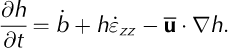
For a glacier that is in steady state, all terms in Equation (10) are temporally invariant and ∂h/∂t =0. Rearranging Equation (10) gives

which is satisfied when

Equation (12) is found by assuming that the velocity vector points in the direction of largest thickness gradient.
Finally, evaluating Equation (12) at or near the terminus and inserting the result into Equation (2) yields

where H 0 is terminus thickness. Equation (13) suggests that ice thickness, strain rate, thickness gradient, mass-balance rate and melting of the vertical face of the terminus are the primary controls on calving rate. All calving models must be consistent with Equation (13) under steady-state conditions.
3.2. Discrete calving
Under steady-state conditions, the position of a glacier terminus is fixed, and thus calving events must occur continuously and be infinitesimally small. We now consider how the mean calving rate is affected by discrete calving events that occur periodically and are always the same size. Near-terminus glacier strain rates, mass-balance rate and submarine melt rate are held constant, but dX/dt ≠ 0. We furthermore assume that terminus advance and retreat occurs parallel to the direction of the largest thickness gradient.
The length vector, Δx, that a point along the terminus retreats during a calving event is given by

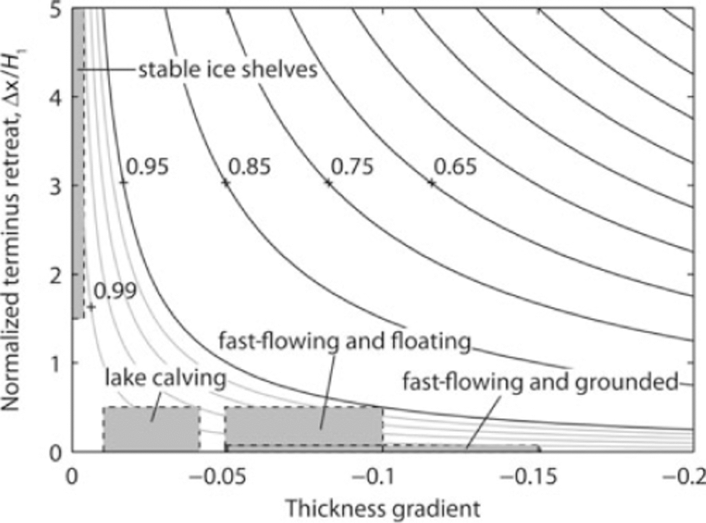
where H 0 is now the terminus thickness at the onset of calving events and H 1 is the terminus thickness immediately following calving events. The curves in Figure 2 show the relationship between H 0/H1, thickness gradient and the distance that a terminus retreats during a calving event.
Contours of H 0/H1 for various along-flow thickness gradients (∂h/∂x) and normalized calving retreat lengths (Δx/H 1). The coordinate system is oriented in the direction of largest thickness gradient. The contours are derived from Equation (14). Gray contours represent intervals of 0.01. Shaded boxes indicate approximate thickness gradients and calving event sizes (see section 4.1).
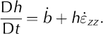
The thinning rate of a column of ice as it is advected toward the terminus is given by the material derivative

We again assume u s = u b = ū, so that ∂h/∂t is given by Equation (10). Inserting Equation (10) into Equation (15) gives
The time interval between calving events, Δt, is determinedstable ice shelves by the time it takes the terminus to thin to H0
. As the terminus thins it also melts backward at some rate, , thus delaying the onset of the next calving event;the column of ice that reaches the terminus at time Δt will have had an initial thickness of  . Integrating Equation (16) from to H
0 gives
. Integrating Equation (16) from to H
0 gives

Equation (17) is implicit. Δt must either be solved iteratively or approximated with a Taylor series expansion. Rearranging Equation (17), we can write

Now, expanding about Δt= 0 and dropping terms containing Δt 2 and higher, we find that

Finally, solving for Δt gives

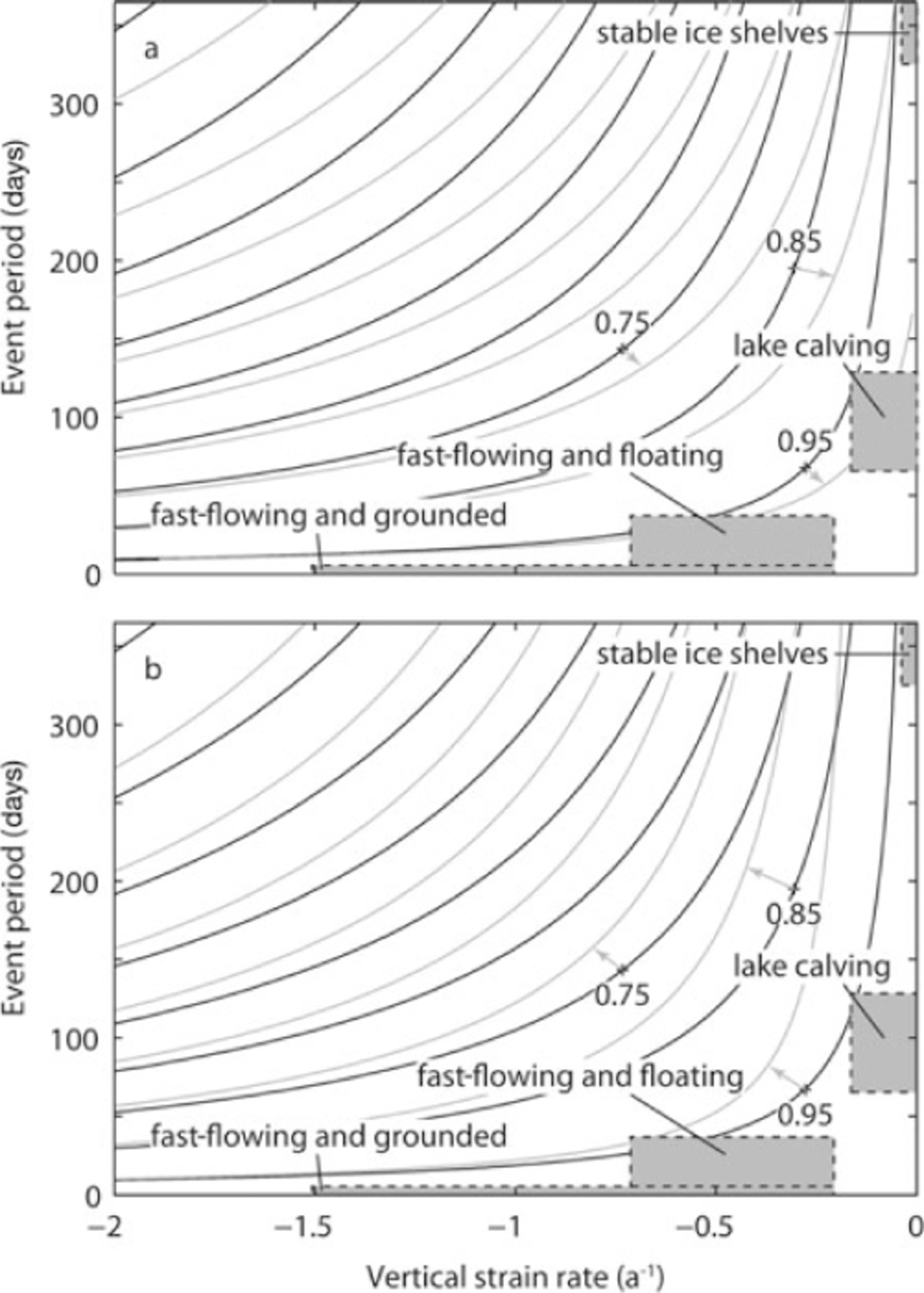
The period between events depends inversely on vertical strain rate and becomes infinitesimally small as H
1 → H
0. When strain rates are high, the ratio of pre- to post-calving terminus thickness, H
0/H
1, has little impact on the time period between events (Fig. 3). Furthermore, melt-induced changes in terminus geometry most strongly impact the calving interval of slowly deforming glaciers; bottom and surface melting  tends to decrease Δt (Fig. 3a), whereas melting of the vertical face of the terminus
  tends to increase Δt (Fig. 3b).
Contours of H
0/H1 for various strain rates , time periods between calving events (Δt), ice thicknesses (H1), mass-balance rates () and melt rates on the vertical face of the terminus The coordinate system is oriented in the direction of largest thickness gradient. The contours are derived from Equation (17). In both panels, H
1 =500m, ∂h/∂x = −0.2 and black curves indicate  . Gray curves indicate that (a)
  and = 0 (surface and bottom melting dominate over backwards melting of the terminus) and (b) = 0 and
  (backwards melting of the terminus dominates over surface and bottom melting). Shaded boxes indicate approximate strain rates and calving intervals (see section 4.1).
Over several calving events, the mean calving rate is

We find, upon inserting Equations (14) and (20) into Equation (21), that the mean calving rate is largest for glaciers that regularly experience large calving events. For example, taking  and
and  , Equation (21) becomes

For a given ice thickness, u c increases with decreasing H 0/H1 (increasing event size). This is because, for a given strain rate, thick ice deforms more rapidly (in an absolute sense) than thin ice (see Equation (16)). Furthermore, when calving events cause up-glacier acceleration (as observed by Reference Amundson, Truffer, Luthi, Fahnestock, West and MotykaAmundson and others, 2008; Reference NettlesNettles and others, 2008) and drawdown, then the mean calving rate should be expected to further increase.
Finally, the limit of u c (Equation (21)) as H 1 → H 0 has an indeterminate form, since both Δx → 0 and Δt → 0. Upon applying l’Hôpital’s rule once and evaluating the limit, Equation (21) reduces to Equation (13), indicating that calving has become continuous and thus demonstrating that our proposed calving framework is consistent with the steady-state scenario, as desired.
3.3. Comparison with an empirical calving relation
The form of our steady-state calving rate relation (Equation (13)) is in strong agreement with the empirical relationship for ice-shelf calving found by Reference AlleyAlley and others (2008). By analyzing data from a variety of ice shelves, they found that the calving rate (along a glacier flowline) could be estimated by

where u c is set equal to terminus velocity u t, w is ice-shelf half-width and c is an empirically determined constant approximately equal to 0.016m-1. All parameters were measured within a few ice thicknesses of the terminus.
Using theoretical work and comparing the results to observations, Reference SandersonSanderson (1979) demonstrated that ice-shelf half-width is related to along-flow thickness gradient, ∂h/∂x< 0, through the relationship
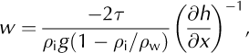
Where τ is the depth-averaged shear stress on the ice-shelf margin, ρi and ρw are the densities of ice and water, g is gravitational acceleration and x points in the down-glacier direction. Inserting Equation (24) into Equation (23) and setting τ = 90kPa (as also done by Reference SandersonSanderson, 1979) gives

When melt terms and across-flow normal strain rates are negligible , , , and thus  the value of u
c in Equation (25) is roughly two to three times greater than our calving rate relation, but the forms of the equations are otherwise identical.
the value of u
c in Equation (25) is roughly two to three times greater than our calving rate relation, but the forms of the equations are otherwise identical.
The factor of two to three difference could be attributed to approximations in the theoretical work of Reference SandersonSanderson (1979) (such as the assumption that ice-shelf thickness does not vary laterally), overestimation of shear stresses on the ice- shelf margin (Reference Crabtree and DoakeCrabtree and Doake (1982), used τ = 40kPa), not accounting for variations in ice-shelf density, our assumption that near-terminus glacier strain rates are steady and spatially invariant and Reference AlleyAlley and others’ (2008) neglecting the importance of lateral strain and mass-balance rate. Furthermore, measurements used by Reference AlleyAlley and others (2008) may have been made farther away from the terminus than is required by Equation (13). For example, the strain rates they cite for Jakobshavn Isbræ are roughly a factor of two smaller than was observed within a few kilometers of the terminus in the 1980s, as suggested by aerial photo- grammetry (R.J. Motyka, unpublished information);if applied uniformly, a factor of two increase in near-terminus strain rate would result in a reduction of c by one-half.
Our steady-state calving rate relation is derived from first principles and accounts for changes in terminus thickness due to lateral stretching, mass-balance rate and backwards melting of the terminus; it is therefore an improvement over the work of Reference AlleyAlley and others (2008). Furthermore, our analysis applies for both grounded and floating termini, potentially explaining Reference AlleyAlley and others’ (2008) observation that the calving rate of Columbia Glacier, Alaska, (a grounded tidewater glacier) was consistent with their linear regression on ice shelves. When applying our calving rate relation, all terms should be evaluated within a few ice thicknesses of the terminus.
4. Physical Interpretation
The functions defining the proposed calving framework, H 0 and H 1, are unknown. They are likely to depend on a number of glaciological and oceanographic parameters, such as strain rates, crevasse depth and crevasse spacing, ice temperature, pre-existing microfractures or ‘damage’ (Pra-Reference Pralong and Funklong and Funk, 2005), meltwater ponding on the glacier surface, terminus proximity to flotation, tides or other ocean swell, and resistance from a cover of proglacial sea ice or ice melange. H 1 furthermore allows for self-sustaining calving processes (positive feedbacks), such as rapid stress transfer due to loss of resistance along the fjord walls or bottom, disintegration of the terminus by glaciogenic ocean waves (Reference MacAyeal, Okal, Aster and BassisMacAyeal and others, 2009), or failure of a resistive ice melange during the onset of a calving event (Reference Amundson, Brown, Truffer, Luthi and MotykaAmundson and others, 2010). In other words, this framework allows calving events to be triggered at any point along the terminus;once triggered, positive feedbacks can cause subsequent calving at distant points on the terminus or up-glacier from the initial rupture. Although H 0 and H 1 are not given here, they can be specified later, once our understanding of the relationship between terminus thickness and calving processes has improved.
In the following subsections, observations from a variety of calving margins are compared to the theoretical analysis in section 3 to gain a rough empirical understanding of the relationship between H 0 and H 1. The relationship is then formulated in terms of physical processes with the aim of identifying future areas of investigation.
4.1. Case studies
Calving glaciers vary in flow speed, ice temperature and geometry. Variations in these parameters give rise to differences in size and frequency of calving events. To investigate appropriate values for H 0/H1, we group calving glaciers into five categories: fast-flowing and grounded (e.g. Alaska tidewater glaciers), fast-flowing and floating (e.g. many outlet glaciers in Greenland), lake calving, stable ice shelves, and unstable ice shelves. Typical near steady-state thickness gradients, calving event retreat lengths, strain rates and periods between calving events for each of these groups, excluding unstable ice shelves, are indicated in Figures 2 and 3. Only approximate ranges are given, as statistics of calving margins are poorly known, poorly documented and often incomplete. For example, strain rates and thickness gradients are often known, but detailed information on calving event size and repeat period is lacking. For some measured values of strain rates and thickness gradients as well as statistics of calving margins, see references in Reference Benn, Warren and MottramBenn and others (2007b), as well as Reference SandersonSanderson (1979), Reference AlleyAlley and others (2008), Reference Amundson, Truffer, Luthi, Fahnestock, West and MotykaAmundson and others (2008), Reference JoughinJoughin and others (2008b) and Reference Walter, O’Neel, McNamara, Pfeffer, Bassis and FrickerWalter and others (2010).
Calving events from grounded glaciers tend to be small but occur frequently (e.g. Reference O’Neel, Echelmeyer and MotykaO’Neel, 2003, Reference O’Neel, Marshall, McNamara and Pfeffer2007), indicating that H 0/H1 ≈ 1. When near-terminus thinning rates are sufficiently large, the terminus will go afloat and H 0/H1 will decrease to 0.96–0.99, regardless of ice temperature (strength), thickness gradient and glacier width, and salinity of the water body (Figs 2 and 3). Note that both temperate lake-calving (Reference Naruse and SkvarcaNaruse and Skvarca, 2000;Reference Warren, Benn, Winchester and HarrisonWarren and others, 2001;Reference Boyce, Motyka and TrufferBoyce and others, 2007) and temperate tidewater glaciers (Reference Walter, O’Neel, McNamara, Pfeffer, Bassis and FrickerWalter and others, 2010) have been observed to develop short floating tongues.
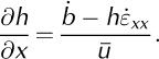
In the calving framework, catastrophic disintegration of unstable ice shelves over a period of days to weeks (Reference Rott, Skvarca and NaglerRott and others, 1996; Reference Scambos, Hulbe, Fahnestock and BohlanderScambos and others, 2000;Reference Braun and HumbertBraun and Humbert, 2009;Reference Braun and HumbertBraun and others, 2009) can occur either through changes in ice-shelf thickness gradient or by decreasing H 0/H1. Variations in ice-shelf thickness gradient can be estimated by considering steady-state profiles of ice shelves, which we generate by assuming that ū = u s, that ice-shelf density is constant and that transverse variations in ice thickness and velocity are small. The steady-state mass continuity equation (Equation (11)) is rearranged and oriented along a glacier flowline, such that
The longitudinal strain rate is found by balancing the total force on any vertical column in the ice shelf with the horizontal force acting on the terminus (see Reference WeertmanWeertman, 1957; Reference SandersonSanderson, 1979), yielding

where A and n are flow-law parameters and L is the total length of the ice shelf. Equations (26) and (27) can be solved by specifying a velocity and thickness at the grounding line, making an assumption about the value of the integral in Equation (27), integrating outward from the grounding line, and iterating until the ice shelf has the desired length (see explanation of methodology by Reference Crabtree and DoakeCrabtree and Doake, 1982).
For an ice shelf with specified width, length and flow-law parameters, ice thickness is determined by thickness and velocity at the grounding line, surface and/or bottom mass- balance rates, and shear stresses on the shelf margins. The geometry of the inner shelf is most strongly influenced by thickness and velocity at the grounding line, whereas the geometry of the outer shelf is determined by balance rate and shear stresses on the shelf margins (both assumed spatially constant) (see Fig. 4). Regardless of the input parameters, the near-terminus thickness gradient of a long ice shelf is nearly constant. Thus for a model to cause an ice shelf to disintegrate, H 0 /H 1 must decrease considerably. Furthermore, processes that may condition an ice shelf for catastrophic, nearly instantaneous failure, such as thinning due to increased melt rates or loss of shear stresses at the margin, may actually steepen the ice shelf and thereby reduce the likelihood that a high value of H 0 /H 1 will cause the ice shelf to fail. Steepening due to increased melting or loss of buttressing forces can initiate a runaway retreat over longer timescales, however, as these processes can increase longitudinal strain rates and associated calving rates.
Theoretical steady-state thickness profiles of a 20 km wide and 100 km long ice shelf for various grounding line thicknesses and velocities (H
g and u
g; see Fig. 1), melt rates () and lateral shear stresses (τ). (a) H
g = 200–1200 m, u
g = 400m a–1, and ττ= 0. (d) H
g = 1000 m, u
g = 200–600m a–1, and τ = 0. (c) H
g = 1000 m, u
g = 400ma–1,  and τ τ 0. (d) H
g τ 1000 m, u
g τ 400ma–1, and τ τ 0–25 kPa. In all plots the thick black curves indicate the points at which H
0/H
1 = 0.95 and 0.98.
and τ τ 0. (d) H
g τ 1000 m, u
g τ 400ma–1, and τ τ 0–25 kPa. In all plots the thick black curves indicate the points at which H
0/H
1 = 0.95 and 0.98.

The above observations suggest the use of the following simple relationship between H 0 and H1 as a starting point for developing a universal calving law:

Equation (28) is, however, too simple to characterize seasonal and other temporal variations in calving rate (see section 5). Furthermore, the point at which an ice shelf becomes unstable is unknown and requires further investigation, but is likely to be related to ice thickness, air temperature and surface melting (e.g. Reference Scambos, Hulbe, Fahnestock and BohlanderScambos and others, 2000).
As a glacier advances or retreats over annual timescales, the relationship between H 0 and H 1 may vary quasiperiodically. For example, for a grounded tidewater glacier, H 0/H1 ≈ 1 and calving events are small but occur frequently. As the terminus retreats and thins it may reach flotation, causing H 0/H 1 to decrease. If the newly formed shelf is structurally rigid, H 0/H1 may only decrease slightly (to ˜0.98) and the shelf will be a meta-stable feature that occasionally calves large icebergs. As the terminus continues to retreat and thin, the floating shelf may become unstable and H 1 will increase. The ice shelf may then catastrophically collapse back to the grounding line, at which point H 0/H1 → 1.
Our calving framework does not preclude the formation of floating shelves during glacier advance. It does require, however, that for an ice shelf to develop during advance the terminus must be thick, slowly flowing (such that the ice is not highly damaged) and cold (with the assumption that cold ice is inherently stronger than warm ice). Otherwise, self-sustaining processes will cause the shelf to collapse immediately after it forms. Possibly, expansive floating shelves are only a relict of retreating ice sheets. At the very least, the length that an ice shelf grows during advance is likely to be limited by the terminus thickness, which is a function of grounding-line thickness and velocity (Reference SandersonSanderson, 1979).
4.2. Toward a physically based description of the calving framework
We ultimately desire a more comprehensive, descriptive relationship between H 0 and H 1 than that suggested in the previous subsection. One such possibility is

where x c is crevasse spacing, Γ ≥ 0 is a function that describes the effect of self-sustaining calving processes (Γ ≈ 0 for grounded termini), T is ice temperature and H g is the ice thickness at the grounding line. For floating termini, the calving flux may be primarily controlled by the propagation of widely spaced rifts, and thus x c refers to rift spacing. (Rift herein refers to a crevasse that penetrates the entire glacier thickness.)
The three terms on the right-hand side of Equation (29) represent three poorly known functions; identification of these functions would lead to a complete calving model. Previous work has focused primarily on identifying H0 (Reference Van der VeenVan der Veen, 1996; Reference Vieli, Funk and BlatterVieli and others, 2001, Reference Vieli, Jania and Kolondra2002; Reference Benn, Hulton and MottramBenn and others, 2007a, Reference Benn, Warren and Mottramb). Although the model of Reference Benn, Hulton and MottramBenn and others (2007a, Reference Benn, Warren and Mottramb) allows ice shelves to form, it does not take into account the potential role of crevasse spacing: if crevasses are widely spaced, then a terminus must reach flotation prior to calving. Although we do not propose an exact formulation for H 0, we do suggest that if |xc | is large, then

where H w is the water depth at the terminus. Thus glaciers with large crevasse spacing (as proposed for lake-calving glaciers; Reference VenterisVenteris, 1999) would be forced to go afloat prior to calving. This requirement does not necessarily force glaciers with small crevasse spacing to remain grounded. For example, if ice thickness is much greater than crevasse depth, crevasses may be ineffective at separating ice blocks from the glacier and a terminus can go afloat faster than it retreats back to the grounding line. In such cases, the calving rate may be more strongly controlled by the growth of deep rifts that penetrate the entire glacier thickness and produce large icebergs, such as those observed at Jakobshavn Isbræ.
The second term in Equation (29) determines the size of a calving event when event size is determined exclusively by crevasse spacing (i.e. when self-sustaining processes are unimportant). In other words, the first crevasse/rift up-glacier from the terminus determines the size of the calving event. This term likely explains why a small range of H0/H1(˜0.96−0.99) may adequately characterize a wide range of calving margins (Figs 2 and 3), as steep, fast-flowing glaciers may be expected to have smaller crevasse/rift spacing than flat, slow-flowing glaciers. Further work, possibly using numerical models of glacier termini, is needed to investigate and parameterize the relationship between glacier geometry, stress field and crevasse/rift spacing.
Finally, the third term in Equation (29) describes the impact of self-sustaining processes. If a glacier has low strain rates and therefore little damage, is thick and/or cold, selfsustaining processes are unlikely to be important and therefore Γ ≈ 0. Γ can increase if these properties change or if a strong melt season causes meltwater to pond in crevasses and force the crevasses to grow downward (see Reference Scambos, Hulbe, Fahnestock and BohlanderScambos and others, 2000). Since self-sustaining processes cannot cause a glacier to retreat far past its grounding line, Γ < H g - H 0 . Furthermore, r may vary seasonally. Such variations may occur at glaciers that develop weak floating tongues during winter but calve from grounded (or nearly grounded) termini in summer (such as Jakobshavn Isbræ).
5. Application of the Calving Framework
The calving framework proposed in section 2 is highly versatile and can easily incorporate new or existing calving models. To demonstrate, we use ad hoc functions for H 0 and H 1 to produce seasonal variations in terminus behavior.
Many tidewater glaciers experience large seasonal variations in terminus position and, in some cases, the size of and time interval between calving events (Reference Meier, Rasmussen, Krimmel, Olsen and FrankMeier and others, 1985; Reference Motyka, Hunter, Echelmeyer and ConnorMotyka and others, 2003;Reference Amundson, Truffer, Luthi, Fahnestock, West and MotykaAmundson and others, 2008, 2010;Reference JoughinJoughin and others, 2008c). Seasonal variations in terminus position can be attributed to variations in calving rate due to changes in thinning rate or thickness gradient, and to variations in backwards melting of the vertical face of the terminus, a process that also enables calving (Reference Vieli, Jania and KolondraVieli and others, 2002; Reference Motyka, Hunter, Echelmeyer and ConnorMotyka and others, 2003; Reference RöhlRöhl, 2006). Variations in the size of and interval between calving events, however, may be better described by processes controlling the ratio of pre- to post-calving terminus thickness (H0/H1; see Figs 2 and 3).
To illustrate the effect of variations in H 0/H1, we arbitrarily pick parameters to describe glacier flow (terminus velocity, strain rate and thickness gradient are held constant) and let H 0 vary sinusoidally. Processes that might cause seasonal variations in H 0 include longitudinal stretching and surface melting, which affect crevasse depth near the terminus (e.g. Reference Benn, Hulton and MottramBenn, 2007a, Reference Benn, Warren and Mottramb), and variations in the strength of buttressing sea ice and/or ice melange (Reference Amundson, Brown, Truffer, Luthi and MotykaAmundson and others, 2010). In cases where calving ceases during winter, H 0 decreases considerably, so that no amount of thinning will cause the terminus to become unstable and calve.
We consider both the case in which H 1 is constant and so H 0/H1 also varies with time, and the case in which H 1(t) = H 0(t) (self-sustaining processes are unimportant). In the former, terminus position is determined by setting terminus velocity equal to some constant value and tracking the interval and size of calving events through Equations (14) and (17). In the latter, calving events occur continuously and are infinitesimally small; we thus use Equation (13) to calculate the instantaneous calving rate. The terminus position at a given time is then found by inserting Equation (13) into Equation (1) and integrating (Fig. 5). Note that although we calculate the instantaneous calving rate using an equation derived from steady-state assumptions, we do not require the terminus position to remain fixed (i.e. dX/dt ≠ 0).
Relative terminus position of a glacier that has u
t=10kma–1,  ∂h/∂x =−0.1(rough values for rapidly flowing outlet glaciers in Greenland), and
  The coordinate system is oriented in the direction of largest thickness gradient. (a) The critical thickness for the onset of calving, H0, varies sinusoidally with an amplitude of 100m and a mean value of
  The troughs represent winter conditions. (b) Seasonal variations in glacier terminus position when H
1 = max(H0(t)) + 10m (black curve) and when H
1(t) =H0(t) (gray curve).
The troughs represent winter conditions. (b) Seasonal variations in glacier terminus position when H
1 = max(H0(t)) + 10m (black curve) and when H
1(t) =H0(t) (gray curve).
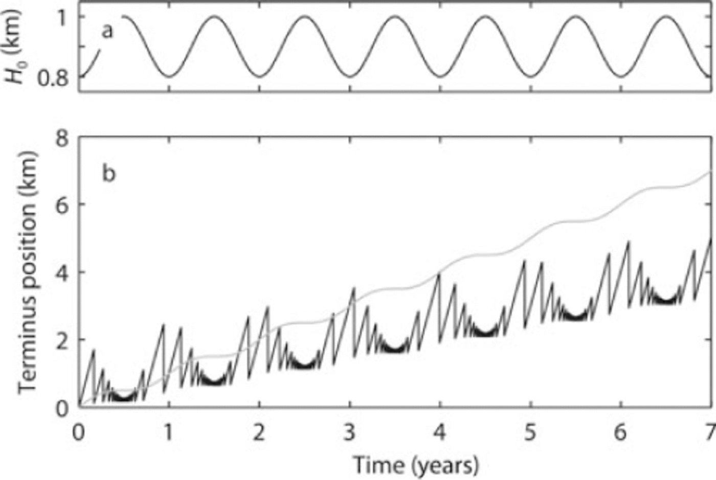
When self-sustaining calving processes are important (H1(t) ≠ H 0(t)), seasonal variations in terminus position are amplified and the model produces fewer but larger calving events in winter than in summer and slightly more calving events in spring than in fall. Also, ignoring selfsustaining processes when they may be important can reduce the mean calving rate by several percent. Our analysis has assumed, however, that terminus velocity is constant and unaffected by changes in terminus position, when in fact glacier velocity has been observed to change as a result of individual calving events (Reference Amundson, Truffer, Luthi, Fahnestock, West and MotykaAmundson and others, 2008; Reference NettlesNettles and others, 2008). These short-term changes in glacier flow associated with calving can influence longterm trends in terminus behavior. Furthermore, changes in the seasonal advance/retreat cycle can affect terminus stability and long-term behavior by enabling a terminus to advance to a stable pinning point in winter or to retreat past a pinning point in summer.
The seasonal variations in terminus position investigated here were driven by processes that control the critical terminus thickness for calving, H 0 (e.g. variations in the buttressing forces from a proglacial ice melange might have this effect; Reference JoughinJoughin and others, 2008a; Reference Amundson, Brown, Truffer, Luthi and MotykaAmundson and others, 2010). A glacier can also experience variations in terminus position when H 0 is held constant. For example, submarine melting of a terminus affects terminus position by influencing the rate at which the terminus thins to H 0. The gray curve in Figure 5, produced by varying H 0 sinusoidally and assuming that H 0= H 1, can also be produced by holding H 0 constant and letting b vary from −100 to +100 m a-1 (see Equation (13)). We thus suggest that ocean temperatures can affect calving both (1) indirectly by influencing the strength of proglacial ice melanges through the growth and decay of interstitial sea ice and (2) directly by influencing the structural rigidity of the terminus (e.g. by controlling the crevasse-depth to ice-thickness ratio).
6. Conclusions
We have developed a framework for iceberg-calving models based on (1) mass continuity, (2) the observation that, over annual timescales, terminus velocity and calving rate are generally much larger than changes in terminus position, suggesting a coupling between calving and flow parameters (Reference Van der VeenVan der Veen, 1996), and (3) the simple idea that terminus thickness is larger following a calving event than immediately preceding the event. Our steady-state analysis indicates that calving rate is primarily governed by ice thickness, thickness gradient, strain rates and melting of the terminus; the analysis also provides a physical explanation for the empirical relationship for ice-shelf calving found by Reference AlleyAlley and others (2008). Furthermore, variations in calving event size and periodicity can be prescribed simply by increasing the terminus thickness (by a few percent or less) during a calving event.
In the calving framework, terminus thicknesses at the onset of and immediately following calving events are given by two unknown but related functions (H0 and H 1, respectively). The functions may depend on strain rates and crevasse spacing, ice temperature, terminus proximity to flotation, tides or other ocean swell, and resistance from proglacial sea ice or ice melange. Furthermore, differences between the functions determine how crevasse spacing and/or self-sustaining processes affect terminus behavior. For well-grounded glaciers with large crevasse spacing, the difference between the two functions depends only on crevasse spacing; if crevasse spacing is large, a terminus may need to achieve flotation prior to calving. However, the functions may differ significantly for floating termini that are thin, highly damaged and/or warm; such termini are unstable to small perturbations and are therefore unlikely to be long-lasting features. With this calving framework, it may be difficult to develop expansive ice shelves during glacier advance, unless the glacier is thick, slowly flowing and cold.
The proposed calving framework does not constitute a complete calving model. It can, however, easily incorporate new or existing thickness-based calving models. The framework is sufficiently general to be applicable to all calving margins, yet sufficiently detailed to give insights into longterm terminus dynamics. Additionally, the form of the functions defining the framework can be investigated through statistical analyses of calving margins or numerical application of ad hoc functions. For example, although H 0 and H 1 may be difficult to measure, it should be possible to estimate the ratio, H 0/H1, by combining our theoretical analysis with measurements of thickness gradient, strain rates, and size and periodicity of calving events. Temporal variations in H 0/H1 can then be compared with other time series to investigate the effect that various processes have on H 0/H1.
Finally, deficiencies in the proposed framework highlight several processes that should be further investigated and parameterized prior to implementing the framework in glacier and ice-sheet models. These include (1) assessment and parameterization of rapid dynamic changes associated with sub-grid and sub-time-step calving events, (2) parameterization of the relationship between glacier geometry, flow and crevasse/rift spacing, and (3) development of a predictive stability criterion for ice shelves.
Acknowledgements
Support for this project was provided by NASA’s Cryospheric Sciences Program (NNG06GB49G), the US National Science Foundation (ARC0531075 and ARC0909552) and an International Polar Year student traineeship funded by the Cooperative Institute for Arctic Research (CIFAR) through cooperative agreement NA17RJ1224 with the US National Oceanic and Atmospheric Administration. The paper was inspired by discussions with E. Bueler, M. Fahnestock, M.P. Luthi, R.J. Motyka, J. Brown and D. Podrasky. We thank A. Vieli, an anonymous reviewer and the scientific editor, R. Greve, for thorough reviews that helped to focus the manuscript.



