


1. Introduction
Over the past few decades, there has been a global trend toward financial globalization, which despite being driven by the intention to direct resources to their most productive destinations, has led to higher volatility in financial markets, global imbalances, and a global financial cycle that disproportionately affects emerging economies (Rey, Reference Rey2015; Miranda-Agrippino and Rey, Reference Miranda-Agrippino and Rey2020). To address these issues, policymakers have implemented new macroprudential regulations such as those in the Basel Accords, and established new institutions, including the Financial Stability Board. The effectiveness of these regulations has been extensively evaluated, along with their broader effects, leakages, and externalities.Footnote 1 However, although observed empirically, these leakages are less understood in terms of their functioning and driving mechanisms (Forbes, Reference Forbes2021); for example, it would be relevant to understand their nature or what generates them, and whether they create additional unaccounted vulnerabilities or, perhaps, the space for welfare improving policy adjustments.
In this study, we develop a macroeconomic framework to explore these regulatory leakages and related questions. We focus on an open economy environment where several emerging economies interact with a common financial center in global markets.Footnote 2 For these economies, the international consequences of nationally implemented regulations are particularly relevant, given their increased fragility to the shocks of global markets (Chang and Velasco, Reference Chang and Velasco2001; Reinhart and Rogoff, Reference Reinhart and Rogoff2009). As policymakers recognize the borderless effects of their implementation, regulations in different locations may become interdependent, prompting policymakers to react with their own toolkit in response. As a result, policy frameworks that internalize such cross-border linkages could be better poised for managing the fluctuations dictated by global financial while better balancing the costs and trade-offs of regulation.Footnote 3
We investigate the nature of international policy spillovers and how they are shaped by the presence of financial frictions and the direction of the policy leakages. Our study is innovative in that we explore a framework with multiple peripheries that jointly can become a relevant entity for their common financial center but that still depend financially on the latter economy given it acts—through their banking sector—as a global creditor. In this setup, the regulators trade-off their incentives to mitigate their financial frictions with those of boosting financial intermediation, and their resulting actions will potentially impact the economic conditions in other locations.
We consider the presence of the banking sector explicitly in our framework along the lines of Gertler and Kiyotaki (Reference Gertler, Kiyotaki, Gertler and Kiyotaki2010), Gertler and Karadi (Reference Gertler and Karadi2011), Adrian and Shin (Reference Adrian, Shin, Adrian and Shin2010), but extended to an open economy environment as in Céspedes et al. (Reference Céspedes, Chang and Velasco2017), with the difference that we allow for a multiperipheral economic structure.Footnote 4 Therefore, this work is related to the studies exploring whether changing financial conditions increase the extent of policy interdependency (e.g., in Fujiwara and Teranishi, Reference Fujiwara and Teranishi2017; Banerjee et al. Reference Banerjee, Devereux and Lombardo2016; Agénor et al. Reference Agénor, Jackson, Kharroubi, Gambacorta, Lombardo and Silva2021).Footnote 5 We build on these studies with a focus on macroprudential interventions and potential cross-border linkages between different types of financially integrated economies.
To introduce a meaningful role for prudential policies, we consider a setup with financial frictions caused by a limited enforcement agency distortion as described by Gertler and Karadi (Reference Gertler and Karadi2011) and Mendoza (Reference Mendoza2010), which will be more prevalent in emerging markets and leads to a default premium on interbank lending relationships, amplifying the scale of financial intermediation, and potentially shaping the international financial spillovers. We examine the existence and nature of cross-border policy spillovers and evaluate the effectiveness of several policy regimes in mitigating this distortion and smoothing the credit spreads. Specifically, we consider a macroprudential instrument that taxes banking sector revenues, similar to Agénor et al. (Reference Agénor, Jackson, Kharroubi, Gambacorta, Lombardo and Silva2021). It is worth noting that this policy tool may impact capital flows across borders and could be seen as a form of capital control. However, we argue that it is better described as a macroprudential tool with potential capital flows implications. To see this, we first demonstrate that it is equivalent to a leverage-ratio requirement, and secondly, we note that it primarily regulates the scale of financial intermediation, which could be international or domestic, without significant effects on capital flows.Footnote 6
Our framework is set as a large open economy model similar to Banerjee et al. (Reference Banerjee, Devereux and Lombardo2016), or Agénor et al. (Reference Agénor, Jackson, Kharroubi, Gambacorta, Lombardo and Silva2021), but with the abstraction from monetary policy concerns. This simplification enables us to extend the environment to that of a multiperipheral financially integrated economy, facilitating the examination of strategic interactions between macroprudential regulators in different types of economies. The consideration of a large open economy is relevant when studying potential prudential leakages; even under the standard assumption that financial centers’ regulators are not concerned with the policy actions of smaller countries (e.g., as in Jin and Shen, Reference Jin and Shen2020), as it may be the case that emerging countries decide to synchronize their policies at the regional level and generate non-trivial policy leakages in both directions—financial center to peripheral block and vice versa—that planners in each location would want to internalize. Having mentioned this, it should be noticed that the financial center still plays a prevalent role in the global market we consider. Hence, by accounting for such international spillovers dictated by financial centers, our study is also related to the global financial cycle literature (Rey, Reference Rey2015, Reference Rey2016) and to studies on the stabilizing role of financial regulations for emerging economies (Nuguer, Reference Nuguer2016; Cuadra and Nuguer, Reference Cuadra and Nuguer2018).
International policy externalities manifest through several channels. First, the profits of exiting bankers are directly affected by domestic and foreign policy tools, and these changes enter the households’ budgets due to ownership. Second, firms fund their input acquisitions with banking loans, and the costs of these loans depend on the policy instruments. Moreover, there is another relevant externality mechanism that implies an interlink between financial distortions at different locations. This mechanism consists of the general equilibrium effects of implementing a policy action. For example, if a center regulator implements a tightening to decrease the external finance premium locally, she inadvertently decreases the cost of debt in other locations since its creditor banks must be indifferent between funding local and foreign projects in equilibrium; this has the unintended effect of increasing the implied financial frictions, credit spread, and external finance premia abroad, prompting foreign regulators—in debtor countries—to make additional policy adjustments.Footnote 7
Additionally, we find that the impact of policy measures increases with the extent of financial distortions, an outcome that aligns with the conventional wisdom that these policies are more useful in emerging markets (Alam et al. Reference Alam, Alter, Eiseman, Gelos, Kang, Narita, Nier and Wang2025 ; Boz et al. Reference Boz, Unsal, Roch, Basu and Gopinath2020). Other factors influencing these effects include the net foreign asset positions, the price and demand changes in the interbank sector, and the disruption in real production activities, which is a prevalent concern in regulation circles and recent empirical studies (e.g., Richter et al. Reference Richter, Schularick and Shim2019; Kim and Mehrotra, Reference Kim and Mehrotra2022). Importantly, all of these features reflect a policy trade-off faced by the financial regulators—they must balance their intention to mitigate the financial frictions with the impact of more stringent policies on financial regulation. Moreover, the open economy setup allows us to see that such trade-off extends beyond the border of the planner’s jurisdiction. For example, a tighter regulation on an emerging country that curtails intermediation domestically will affect negatively the center economy whose banks’ act as a creditor of the former economy.
To inquire further into the nature of these leakages, we apply another extension where repeated financial intermediation with profits retaining is incorporated into the framework to allow for richer—and more empirically plausible—policy dynamics. In this case, the policy decisions become dynamic in the sense that current policy changes have effects on future balance sheets (and profits) of the banking sector. In this context, the policy effects—direct and leaked across borders—can be magnified, increasing the interdependency of policy across economies.
Finally, we explore the implications of our framework for policy design. We find that optimal policy configurations prompt emerging economies to prioritize mitigating their frictions, while the center reacts by attempting to steer higher intermediation flows toward the peripheries through tighter domestic policies (which in relative terms implies looser lending conditions toward other lenders abroad). These nationally oriented policies imply strong interventions that can be socially costly, which we illustrate by reporting optimal policies for alternative regimes where regulators internalize their effect on the rest of the world’s welfare. In such centralized cases, planners can afford to minimize regulatory wasteful actions by enacting the same effects with more conservative interventions. Importantly, we verify that policies are impactful enough to mitigate the financial friction in all regimes, an outcome that hinges heavily in the flexibility of the policy toolkit in each regime as illustrated by Korinek (Reference Korinek2016). However, when regulation costs potentially affect the toolkit flexibility, the decentralized (nationally oriented) policies, requiring more interventionism, become less capable of achieving a constrained efficient outcome, opening the scope for welfare-inducing coordinated policy frameworks.
There are several strands of literature related to our work. First, our study intends to provide a framework consistent with the empirical findings on macroprudential linkages across borders; these consider the studies on how financial regulation can affect foreign agents and markets (Buch and Goldberg, Reference Buch and Goldberg2017; Forbes et al. Reference Forbes, Reinhardt and Wieladek2017; Forbes, Reference Forbes2021), as well to how prudential policies implementations can leak financial (in)stability to other economies (Aiyar et al. Reference Aiyar, Calomiris and Wieladek2014; Tripathy, Reference Tripathy2020). On the other hand, related literature has produced two-country large open economy frameworks to explore the interdependency of macroprudential regulators, for example, for interactions between regulators in a monetary union (e.g., Rubio and Carrasco-Gallego, Reference Rubio and Carrasco-Gallego2016; Agénor et al. Reference Agénor, Jackson and Jia2021; Dennis and Ilbas, Reference Dennis and Ilbas2023) or for interactions between emerging and advanced economies (e.g., Nuguer, Reference Nuguer2016; Cuadra and Nuguer, Reference Cuadra and Nuguer2018); our framework is similar in exploring regulatory interactions but differs in that it considers a multiperipheral structure that permits us to see which effects arise between seemingly disconnected (emerging) countries that share a common financial center.Footnote 8
On the other hand, to study the implications of the leakages, we explore potential policy design implications for interconnected countries that in principle may choose to coordinate their policy decisions. In that sense, although performing a comprehensive welfare accounting exercise is beyond the scope of our setup, some implications are similar to studies on macroprudential policy cooperation (e.g., Davis and Devereux, Reference Davis and Devereux2022; Korinek, Reference Korinek2016; Bengui, Reference Bengui2014; Jin and Shen, Reference Jin and Shen2020; Kara, Reference Kara2016, among others).Footnote 9 , Footnote 10
The rest of the paper is organized as follows: Section 2 explains the baseline model, Sections 3 and 5 explore the model analytically, initially in our baseline setup and then in an extended version, respectively. Then in Section 4, we describe the numerical solution of the model, and in Section 6, we discuss the policy implications. Finally, we conclude.
2. The model
Our framework is based on Banerjee et al. (Reference Banerjee, Devereux and Lombardo2016), meaning that it essentially follows the banking sector modelation of Gertler and Karadi (Reference Gertler and Karadi2011) applied to an open economy setup. In this paper, however, we introduce a multiperipheral environment, where the peripheric block of the economy is allowed to have several emerging economies that interact with one financial center. At the same time, we include a macroprudential policy in the form of a tax to the return on capital as in Agénor et al. (Reference Agénor, Jackson, Kharroubi, Gambacorta, Lombardo and Silva2021) and Aoki et al. (Reference Aoki, Benigno and Kiyotaki2016), among others. The advantage of this formulation is that the policy instrument will be attached directly to the credit spreads that are augmented by the friction and drive the capital flows at the cross-country level. On the other hand, to keep the model simple, our initial formulation will only consider a simple financial intermediation period, but this is extended in the later sections.Footnote 11
2.1 Economic environment
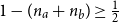
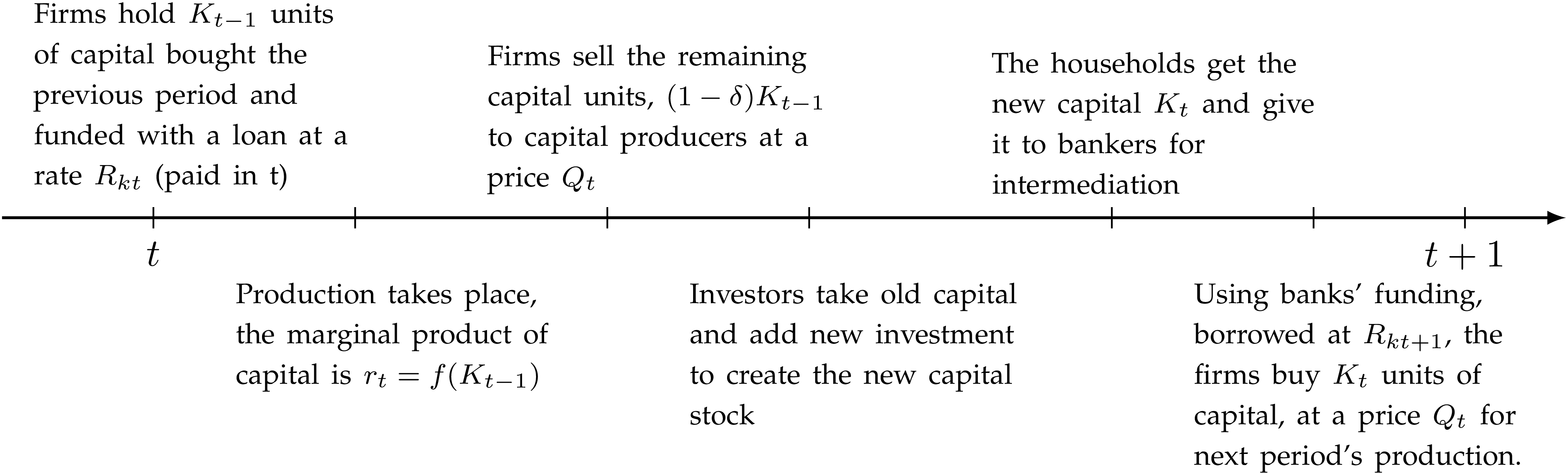
The main feature defining whether a country is an emerging economy is that its financial sector has a limited intermediation capacity, meaning it is unable to issue deposit claims for their households to some extent. As a consequence, it will have to resort to the international financial banking sector to make up for the difference and being able to meet their firms’ funding needs. This environment is depicted in Figure 1, where the red arrows represent financial flows.
Financial flows environment in the model.
Note: All arrows denote financial flows. The blue arrows, in addition, refer to flows that are paid to the banks by their borrowers. This latter type of flow—or specifically the associated rate of return perceived by financial intermediaries—is the one affected by the prudential regulations in the model.

Such structure implies that the emerging economies are financially dependent on the funding from center banks, and in an environment of imperfect information in the lending contracts, this could imply a double layer of agency frictions in the economy: that between center households and banks and another one between global banks and emerging country banks. We also assume the friction is more accentuated in the peripheries.Footnote 12
For simplicity, the real sector will consist only of one consumption good, and there will be no deviations from the law of one price. Preferences are identical between agents, implying the parity or purchasing power holds, and the real exchange rate will be constant (equal to one), playing no role in this version of the model. Additionally, the households will have access to an international market of non-contingent bonds. This is relevant as it implies that, despite the limited capacity to hold deposits, the saving decisions of emerging economies’ households are not curtailed in any way once they trade these assets.
Finally, the lending relationships are subject to a limited enforceability friction which induces an external finance premium and augments the scale of intermediation and credit cycles. The external premium takes the form of an increased return rate for the banks which raises their—expected and eventual—revenues. Such revenues will be targeted by the macroprudential regulation, meaning it will attack the financial friction at its origin.
2.2 Timing and countries setup
The world consists of three economies that live for two periods
 $t=1,2$
. The economies are indexed by
$t=1,2$
. The economies are indexed by
 $i={a,b,c}$
, where the first two will be emerging countries (
$i={a,b,c}$
, where the first two will be emerging countries (
 $a$
and
$a$
and
 $b$
) and the third one is a developed economy that acts as financial center (c). The relative population sizes of the economies are
$b$
) and the third one is a developed economy that acts as financial center (c). The relative population sizes of the economies are
 $n_i$
with
$n_i$
with
 $1-(n_a+n_b) \geq \tfrac {1}{2}$
. Each economy has five types of agents: households, final consumption good producers, capital producers, banks, and a government sector.
$1-(n_a+n_b) \geq \tfrac {1}{2}$
. Each economy has five types of agents: households, final consumption good producers, capital producers, banks, and a government sector.
As mentioned before, preferences across countries’ households are identical, and there is only one final consumption good worldwide that is freely traded and produced in all locations. In terms of notation, superindexes denote the country, while subindexes refer to other features such as the sector of the economy and time periods. Additionally, if a superindex is omitted, it normally means that the variable or equation applies to the three countries.
2.3 Investors
For simplicity, the investment decision is separated from the other household decisions and will be subject to adjustment costs. Physical capital is produced in a competitive market by using old capital and investment. The investment will be subject to convex adjustment costs, with the total cost of investing
 $I_1$
being:
$I_1$
being:
 \begin{equation*} C(I_1) = I_1\left (1 + \frac {\zeta }{2} \left (\frac {I_1}{\bar I}-1\right )^2 \right ), \end{equation*}
where
 $\bar I$
represents the reference level for defining the adjustment cost; The reference level is usually set at the steady state, the previous level of investment, or a combination. In any case, it must hold that
$\bar I$
represents the reference level for defining the adjustment cost; The reference level is usually set at the steady state, the previous level of investment, or a combination. In any case, it must hold that
 $C(0) = 0, \ C''(\! \cdot \!) \gt 0$
. The capital-producing firms (investors) buy back the old capital stock from the firms at price
$C(0) = 0, \ C''(\! \cdot \!) \gt 0$
. The capital-producing firms (investors) buy back the old capital stock from the firms at price
 $Q_1$
and produce new capital subject to the adjustment costs (proportional to the parameter
$Q_1$
and produce new capital subject to the adjustment costs (proportional to the parameter
 $\zeta$
).
$\zeta$
).
The investor solves:Footnote 13
 \begin{equation*} \max _{I_1} \ Q_1 I_1 - I_1\left (1 + \frac {\zeta }{2} \left (\frac {I_1}{\bar I}-1\right )^2 \right )\!, \end{equation*}
the optimality condition (F.O.N.C.) is,
 \begin{equation} [I_1] \, : \qquad Q_1 = 1 + \frac {\zeta }{2} \left (\frac {I_1}{\bar I}-1\right )^2 + \zeta \left (\frac {I_1}{\bar I}-1\right ) \frac {I_1}{\bar I}, \end{equation}
2.4 Firms
Each period, the firms will operate with a Cobb–Douglas technology that aggregates capital predetermined at the end of the period before. This technology of aggregation is given by
 $Y_t = A_t(\xi _tK_{t-1})^\alpha$
, where
$Y_t = A_t(\xi _tK_{t-1})^\alpha$
, where
 $A_t$
is the aggregate productivity and
$A_t$
is the aggregate productivity and
 $\xi$
is a capital-specific productivity or quality term. The capital in
$\xi$
is a capital-specific productivity or quality term. The capital in
 $t=1$
follows standard dynamics with depreciation as,
$t=1$
follows standard dynamics with depreciation as,
 \begin{equation} K_1 = I_1 + (1-\delta ) \xi _1 K_0. \end{equation}
The capital in the initial period will be provided directly by the households in the quantity
 $K_0$
. However, after that, the firm funds physical capital acquisitions for future production (
$K_0$
. However, after that, the firm funds physical capital acquisitions for future production (
 $K_1$
) using lending from the banking sector. Given the model’s timing, there is only one period of intermediation (
$K_1$
) using lending from the banking sector. Given the model’s timing, there is only one period of intermediation (
 $t=1$
) when lending is extended to acquire capital for production in the final period (
$t=1$
) when lending is extended to acquire capital for production in the final period (
 $t=2$
).
$t=2$
).
In this setup, the firms solve a slightly different problem each period. First, they decide how much capital to rent from households:
 \begin{align*} \max _{K_{0}} \ \pi _{f,1} &= Y_1 - r_1 K_{0}, \\[2pt] s.t. \quad & Y_1 = A_1(\xi _1 K_{0})^\alpha , \end{align*}
where
 $r_1$
is the rental rate of capital, which, from the optimality condition, is
$r_1$
is the rental rate of capital, which, from the optimality condition, is
 $r_1 = \alpha A_1\xi _1^\alpha K_{0}^{\alpha -1}$
. For the second period, the firms take into account the cost of funding and the revenue of selling the remaining capital stock to capital good producers that carry out the necessary investment to build the capital stock for the next period. Thus, in the second period, the firm will solve:
$r_1 = \alpha A_1\xi _1^\alpha K_{0}^{\alpha -1}$
. For the second period, the firms take into account the cost of funding and the revenue of selling the remaining capital stock to capital good producers that carry out the necessary investment to build the capital stock for the next period. Thus, in the second period, the firm will solve:
 \begin{align*} \max _{K_{1}} \ \pi _{f,2} &= Y_2 + Q_2 (1-\delta ) \xi _2 K_1 - R_{k,2} Q_1 K_1, \\[2pt] s.t. \quad & Y_2 = A_2(\xi _2 K_{1})^\alpha . \end{align*}
With F.O.N.C.,
 \begin{equation*} [K_{1}]\,: \qquad \alpha A_2 \xi _2^\alpha K_1^{\alpha -1} + (1-\delta ) \xi _2 Q_2 = R_{k,2} Q_1. \end{equation*}
To facilitate the model notation, we follow the same definition for
 $r_2$
, that is,
$r_2$
, that is,
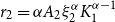 $r_2 = \alpha A_2 \xi _2^\alpha K_{1}^{\alpha -1}$
.
$r_2 = \alpha A_2 \xi _2^\alpha K_{1}^{\alpha -1}$
.
Substituting in the optimality condition for
 $K_1$
, we obtain that the rate paid to the banks by the firms is given by
$K_1$
, we obtain that the rate paid to the banks by the firms is given by
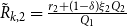 $\tilde R_{k,2} = \tfrac {r_2 + (1-\delta )\xi _2Q_2}{Q_1}$
. Moreover, by taking into account the possibility of a macroprudential tax on the marginal return on capital, such as in Agénor et al. (Reference Agénor, Jackson, Kharroubi, Gambacorta, Lombardo and Silva2021), we have that the effective rate obtained by the banks, that is, after paying the macroprudential taxes (
$\tilde R_{k,2} = \tfrac {r_2 + (1-\delta )\xi _2Q_2}{Q_1}$
. Moreover, by taking into account the possibility of a macroprudential tax on the marginal return on capital, such as in Agénor et al. (Reference Agénor, Jackson, Kharroubi, Gambacorta, Lombardo and Silva2021), we have that the effective rate obtained by the banks, that is, after paying the macroprudential taxes (
 $ \tau r_2 K_1$
) to the government is given by:
$ \tau r_2 K_1$
) to the government is given by:
 \begin{equation} R_{k,2} = \frac {(1-\tau )r_2 + (1-\delta ) \xi _2 Q_2}{Q_1}. \end{equation}
For the sake of clarity, it is important to notice that the firms will pay the pre-taxes banking rate. Only afterward, the banks will consider the effect of the taxes in their profits.Footnote 14 We elaborate on the policy tool and the role of this return rate in later subsections.Footnote 15
2.4.1 Capital dynamics and ownership
The dynamics of the model will be driven (within and cross-country) by the capital flows. For that reason, it is relevant to clarify how capital is held, and profited from, by several types of agents in a single period.
Capital ownership within a period.
Note: This figure describes the ownership of capital across the agents of the model for a generic period
 $t$
. In terms of our baseline model
$t$
. In terms of our baseline model
 $t = 1$
; similarly,
$t = 1$
; similarly,
 $t={1,2}$
for the second setup with two periods of intermediation.
$t={1,2}$
for the second setup with two periods of intermediation.
There is only one period of capital accumulation (
 $t = 1$
). The initial capital will be given for that period as
$t = 1$
). The initial capital will be given for that period as
 $K_0$
. Then, by the end of the accumulation period, the capital in the economy will be given by
$K_0$
. Then, by the end of the accumulation period, the capital in the economy will be given by
 $K_1$
. That capital will be used for the following period’s production. The capital ownership between agents throughout each period is shown in Figure 2, which explains a typical period with intermediation.
$K_1$
. That capital will be used for the following period’s production. The capital ownership between agents throughout each period is shown in Figure 2, which explains a typical period with intermediation.
It should be noticed that the capital used for production in the period
 $t = 1$
cannot be subject to intermediation since there are no banks before the rest of the agents exist (the banks themselves are owned household agents). Therefore, the pre-existing capital stock (
$t = 1$
cannot be subject to intermediation since there are no banks before the rest of the agents exist (the banks themselves are owned household agents). Therefore, the pre-existing capital stock (
 $K_0$
) will be provided directly from households to firms without explicit financial intermediation.Footnote
16
$K_0$
) will be provided directly from households to firms without explicit financial intermediation.Footnote
16
2.5 Banks
This is the target sector of the macroprudential policies. The set up is largely based on Gertler and Karadi (Reference Gertler and Karadi2011). There is a financial intermediation sector in the first period that facilitates funding for firms at the local level. In addition, the bank at the center is also a global creditor and extends loans to banks in other locations. In terms of its functioning, the bank receives a start-up capital by their owner household and will try to maximize the value of the banking activities, given by the present value of its profits. Finally, at the end of its life, the bank will give back their net worth to the households as profits.
There will be a costly enforcement agency friction where it is possible for the banks to divert a portion of the assets they intermediate. The eventual implication of this is the imposition of an external finance premium to the banking revenue rates, which is imposed to prevent the banks from absconding assets and to align their incentives with those of the assets’ owners. This is the financial friction in this environment that augments the credit cycles.
Starting from this section, it will be useful in some cases to use a super index
 $e$
for denoting variables from emerging economies (
$e$
for denoting variables from emerging economies (
 $e=\{a,b\}$
), whereas as before, variables that apply for all countries are either left without a superindex or labeled with an index
$e=\{a,b\}$
), whereas as before, variables that apply for all countries are either left without a superindex or labeled with an index
 $i$
when necessary (e.g., when the same expression involves variables from various locations).
$i$
when necessary (e.g., when the same expression involves variables from various locations).
2.5.1 Emerging countries
The financial system of the emerging countries will have a limited capacity of intermediation of deposits from local households. For simplicity, we assume that there are not any local deposits in these economies, implying that they rely almost entirely on foreign lending from the center banks for providing funding to firms for production. Therefore, the balance sheet of the bank includes, on the asset side, the lending provided to firms, and on the liability and equity side, the foreign lending from center banks and a start-up capital they receive from local households.
The lending relationship between foreign and local banks will be subject to agency frictions, arising from the fact that creditor banks could default on their debt repayment and divert a portion
 $\kappa$
of their intermediated assets.Footnote
17
In either case (default or not), the gross return from intermediation for the bank is
$\kappa$
of their intermediated assets.Footnote
17
In either case (default or not), the gross return from intermediation for the bank is
 $R_{k,2}$
as defined in equation (3).
$R_{k,2}$
as defined in equation (3).
The emerging market bank maximizes its franchise value in the period 1 (
 $J_1$
):
$J_1$
):
 \begin{align} \max _{F_1^e,L_1^e} J_1^e \,= \, \mathbb{E}_1\Lambda _{1,2}^e\pi _{b,2}^e &= \mathbb{E}_1\Lambda _{1,2}^e\big(R_{k,2}^e L_1^e - R_{b,1}^eF_1^e\big), \nonumber \\[4pt] s.t. \quad L_1^e &= F_1^e + \delta _bQ_1^eK_0^e, \\[-2pt] \nonumber \end{align}
 \begin{align} J_1^e &\geq \kappa \mathbb{E}_1\Lambda _{1,2}^e R_{k,2}^eL_1^e, \\[-10pt] \nonumber \end{align}
where
 $L_1^e = Q_1^eK_1^e$
is the total intermediated lending,
$L_1^e = Q_1^eK_1^e$
is the total intermediated lending,
 $F_1^e$
is the foreign interbank lending borrowed from the center bank at a gross rate
$F_1^e$
is the foreign interbank lending borrowed from the center bank at a gross rate
 $R^e_{b,1}$
,
$R^e_{b,1}$
,
 $\delta _bQ_1^eK_0^e$
is the start-up capital received from households, and
$\delta _bQ_1^eK_0^e$
is the start-up capital received from households, and
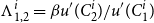 $\Lambda _{1,2}^i = \beta u'(C_2^i)/u'(C_1^i)$
is the stochastic discount factor for a household in country
$\Lambda _{1,2}^i = \beta u'(C_2^i)/u'(C_1^i)$
is the stochastic discount factor for a household in country
 $i$
. At the same time, the constraints correspond to the balance sheet of the bank and an incentive compatibility constraint (ICC) imposing that the value of the bank equals or exceeds the value from defaulting.
$i$
. At the same time, the constraints correspond to the balance sheet of the bank and an incentive compatibility constraint (ICC) imposing that the value of the bank equals or exceeds the value from defaulting.
The F.O.N.C. with respect to the foreign debt is:
 \begin{align} [F_{1}]\,: \qquad (1+\mu ^e)\mathbb{E}_1\Lambda _{1,2}^e\big(R_{k,2}^e-R_{b,1}^e\big) = \mu ^e\mathbb{E}_1 \kappa \Lambda _{1,2}^e R_{k,2}^e, \end{align}
where
 $\mu ^e$
is the Lagrange multiplier of the ICC. This expression is already informative about some implications of the frictions that we explore in propositions at the end of this section.Footnote
18
$\mu ^e$
is the Lagrange multiplier of the ICC. This expression is already informative about some implications of the frictions that we explore in propositions at the end of this section.Footnote
18
2.5.2 Advanced economy
To simplify, we assume there is no agency problems at the center.Footnote 19 Then, the center bank solves:
 \begin{align} \max _{F_1,L_1,D_1} J_1 = \mathbb{E}_1\Lambda _{1,2} \pi _{b,2}^c &= \mathbb{E}_1\Lambda _{1,2}\big(R_{b,1}^aF_1^a + R_{b,1}^bF_1^b +R_{k,2}^c L_1^c - R_{D,1}D_1\big), \notag \\[2pt] s.t. \quad &F_1^a + F_1^b + L_1 = D_1 + \delta _bQ_1^cK_0^c. \end{align}
The only restriction will be the balance sheet of the bank that now counts with the foreign interbank flows on the asset side and the local center deposits on the liability side (
 $D_1$
). Additionally, the deposits from households are subject to a gross rate
$D_1$
). Additionally, the deposits from households are subject to a gross rate
 $R_{D,1}$
.
$R_{D,1}$
.
The associated F.O.N.C.s are:
 \begin{align*} \big[F_1^a\big]\,: \quad \mathbb{E}_1\big(R_{b,1}^a - R_{D,1}\big) = 0, \qquad \big[F_1^b\big]\,: \quad \mathbb{E}_1\big(R_{b,1}^b - R_{D,1}\big) = 0,\qquad \big[L_1^c\big]\,: \quad \mathbb{E}_1\big(R_{k,2}^c - R_{D,1}\big) = 0. \end{align*}
An important consequence of these optimality conditions is that a policy that affects the revenue rate
 $R_{k,2}^c$
will have general equilibrium effects and inadvertently lower the cost of debt for debtor economies (
$R_{k,2}^c$
will have general equilibrium effects and inadvertently lower the cost of debt for debtor economies (
 $R_{b,1}^a, R_{b,1}^b$
). This implies an interaction between the credit spreads and financial frictions between countries that is overlooked by nationally oriented planners.Footnote
20
$R_{b,1}^a, R_{b,1}^b$
). This implies an interaction between the credit spreads and financial frictions between countries that is overlooked by nationally oriented planners.Footnote
20
2.6 Macroprudential policy and public budget
Among the number of possible prudential policiesFootnote
21
(VaR regulations, leverage caps, loan/value ratios, etc.) we consider a general type of policy that, as explained by Agénor et al. (Reference Agénor, Jackson, Kharroubi, Gambacorta, Lombardo and Silva2021), encompasses a broad set of macroprudential regulations: a tax (
 $\tau$
) on the return to capital (
$\tau$
) on the return to capital (
 $R_{k2} = [(1-\tau ^i)r_t+(1-\delta )\xi _2Q_2]/Q_1$
). This will be a tax levied on the banking sector, as shown in Equation (3).
$R_{k2} = [(1-\tau ^i)r_t+(1-\delta )\xi _2Q_2]/Q_1$
). This will be a tax levied on the banking sector, as shown in Equation (3).
Although prudential in nature—as it is implemented on the intermediation sector—the policy tool can also be thought in practice as a device to impose controls on capital flows. This is the case because the tax has the advantage of affecting directly the wedge between the return on capital and borrowing rate (cost of funds for the bank), that is, the credit spread, which in turn drives financial flows at the interbank level. Thus, we are taxing the source of inefficiencies directly.Footnote 22
On the public budget level, this is reflected as a distortionary tax funded with lump sum taxes (
 $T$
) in each period; that is, we assume a balanced fiscal budget,
$T$
) in each period; that is, we assume a balanced fiscal budget,
 \begin{equation*} \tau ^i r_2 K_{1} + T = 0. \end{equation*}
When setting the taxes optimally, each social planner might consider whether to maximize her national welfare or to join cooperative arrangements which would dictate policy centrally.Footnote 23 We explore these cases as an additional exercise in Section 6.
2.7 Households
The households derive utility from consumption and its lifetime utility is given by
 $U = u(C_1) + \beta u(C_2)$
with
$U = u(C_1) + \beta u(C_2)$
with
 $u(C) = \tfrac {C^{1-\sigma }}{1-\sigma }$
. The budget constraints in each period are the following:
$u(C) = \tfrac {C^{1-\sigma }}{1-\sigma }$
. The budget constraints in each period are the following:
Emerging markets:
 \begin{align} C_1^e + \frac {B_1^{e}}{R_1^e} &= r_1^e K_0^e + \pi _{f,1}^e + \pi _{inv,1}^e - \delta _b Q_1^e K_0^e, \\[-10pt]\nonumber \end{align}
 \begin{align} C_2^e &= \pi _{f,2}^e + \pi _{b,2}^e + B_1^e - T^e, \quad for \ e=\{a,b\}, \\[-2pt] \nonumber \end{align}
where
 $C$
is the final consumption good,
$C$
is the final consumption good,
 $B$
a non-contingent internationally traded bond,
$B$
a non-contingent internationally traded bond,
 $r_1$
the rental rate of capital,
$r_1$
the rental rate of capital,
 $Q$
the relative price of capital,
$Q$
the relative price of capital,
 $K$
the capital stock, and
$K$
the capital stock, and
 $T$
is a lump sum tax. Additionally,
$T$
is a lump sum tax. Additionally,
 $\pi$
stands for profits which can come from production activities in final goods (
$\pi$
stands for profits which can come from production activities in final goods (
 $f$
), capital goods (
$f$
), capital goods (
 $inv$
), or banking services (
$inv$
), or banking services (
 $b$
).
$b$
).
Advanced Economy:
 \begin{align} C_1^c + \frac {B_1^{c}}{R_1^c} + D_1 &= r_1^c K_0^c + \pi _{f,1}^c + \pi _{inv,1}^c - \delta _b Q_1^c K_0^c, \\[-10pt] \nonumber \end{align}
 \begin{align} C_2^c &= \pi _{f,2}^c + \pi _{b,2}^c + B_1^c + R_{D,1}D_1 - T^c, \\[12pt] \nonumber \end{align}
where the advanced economy also includes local deposits
 $D$
in the budget constraint as these are intermediated by their banks. Additionally, the profits are given by:Footnote
24
$D$
in the budget constraint as these are intermediated by their banks. Additionally, the profits are given by:Footnote
24
 \begin{align*} \pi _{f,1} &= A_1 \xi _1^\alpha K_0^{\alpha } - r_1 K_{0}\\[2pt] \pi _{f,2} &= A_2 \xi _2^\alpha K_1^{\alpha } + Q_2 (1-\delta )\xi _2 K_1 - R_{k,2} Q_1 K_1\\[2pt] \pi _{inv,1} &= Q_1 I_1 - I_1 \left (1+\frac {\zeta }{2} \left ( \frac {I_1}{\bar I} -1 \right )^2 \right )\\[2pt] \pi _{b,2}^e &= R_{k,2}^e Q_1^e K_1^e - R_{b,1}^e F_1^e, \quad for \ e=\{a,b\} \\[2pt] \pi _{b,2}^c &= R_{b,1}^a F_1^a + R_{b,1}^b F_1^b + R_{k,2}^c Q_1^c K_1^c - R_{D,1} D_1 \end{align*}
In the first period, households maximize their lifetime utility stream subject to the budget constraints for the first and second periods. The F.O.N.C. for the three countries’ households is:
 \begin{align} u'(C_1) \,=\, \beta R_1 \mathbb{E}_1 [u'(C_2)], \qquad u'\big(C_1^c\big) \,=\, \beta R_{D,1} \mathbb{E}_1 \big[u'\big(C_2^c \big)\big], \end{align}
where the first equation is the Euler equation for bonds and applies to the three economies, while the second is the Euler equation for local deposits and holds only for country
 $c$
.
$c$
.
2.8 Market clearing
At the world level, bonds are characterized by zero-net-supply,
 \begin{equation} n_a B_1^a + n_b B_1^b + n_c B_1^c = 0. \end{equation}
The goods market clearing conditions for each period are
 \begin{align*} n_a \left ( C_1^a + I_1^a \left (1+\frac {\zeta }{2} \left ( \frac {I_1^a}{\bar I} -1 \right ) \right ) \right ) + n_b \left ( C_1^b + I_1^b \left (1+\frac {\zeta }{2} \left ( \frac {I_1^b}{\bar I} -1 \right ) \right ) \right )& \\[2pt] + n_c \left ( C_1^c+ I_1^c \left (1+\frac {\zeta }{2} \left ( \frac {I_1^c}{\bar I} -1 \right ) \right ) \right ) = n_a Y_1^a &+ n_b Y_1^b + n_c Y_1^c,\\[2pt] n_a C_2^a + n_b C_2^b + n_c C_2^c = n_a Y_2^a + n_b Y_2^b + n_c Y_2^c \end{align*}
Finally, given that there is only one final good and the law of one price holds (so that the real exchange rate in all cases is one), we have by an uncovered interest rate parity argument that:
 $R_1^a = R_1^b = R_1^c = R_1$
, where
$R_1^a = R_1^b = R_1^c = R_1$
, where
 $R_1$
denotes the world interest rate on bonds in period
$R_1$
denotes the world interest rate on bonds in period
 $1$
.Footnote
25
$1$
.Footnote
25
2.9 Equilibrium
Given the policies
 $\{\tau ^a, \tau ^b, \tau ^c\}$
, the equilibrium consists of prices
$\{\tau ^a, \tau ^b, \tau ^c\}$
, the equilibrium consists of prices
 $\{Q_t^i\}$
, rates
$\{Q_t^i\}$
, rates
 $\{R_1, R_{k,2}^e\}$
and quantities
$\{R_1, R_{k,2}^e\}$
and quantities
 $\{B_1^i, K_1^i, F_1^e, D, C_t^i, I_t^i\}$
for
$\{B_1^i, K_1^i, F_1^e, D, C_t^i, I_t^i\}$
for
 $t=\{1,2\}$
, with
$t=\{1,2\}$
, with
 $i=\{a,b,c\}$
,
$i=\{a,b,c\}$
,
 $e=\{a,b\}$
, such that the households solve their utility maximization problem, the firms solve their profits maximization problems, banks maximize their franchise value, and the goods and bonds markets clear. This allocation is characterized by the solution to the system of equations (1)–(13) where some equations apply for the three economies, other show up by country type, and the clearing condition is considered once (26 equations and variables in total). The simplified system of equations we use to solve the model is summarized in Table A1 in Appendix A.
$e=\{a,b\}$
, such that the households solve their utility maximization problem, the firms solve their profits maximization problems, banks maximize their franchise value, and the goods and bonds markets clear. This allocation is characterized by the solution to the system of equations (1)–(13) where some equations apply for the three economies, other show up by country type, and the clearing condition is considered once (26 equations and variables in total). The simplified system of equations we use to solve the model is summarized in Table A1 in Appendix A.
2.10 Some relevant implications of the model
From this setup, we can already derive a number of important results that can be helpful in understanding the policy implications of the model. First, we can link the extent of the inefficiency—captured by the credit spread—and financial friction to a specific parameter (
 $\kappa$
):
$\kappa$
):
Proposition 1.
If the ICC binds the credit spread is positive and increases in
 $\kappa$
Proof. W.L.O.G. we will work in a perfect foresight setup, otherwise the same result applies to the expected credit spread. From the F.O.N.C. in equation (6), we can obtain:
 \begin{equation*} R_{k,2}^e = \underset {\Phi }{\underbrace {\frac {1+\mu ^e}{1+(1-\kappa )\mu ^e}} }R_{b,1}. \end{equation*}
 $\Phi \gt 1$
represents the proportionality scale between
$\Phi \gt 1$
represents the proportionality scale between
 $R_{k,2}$
and
$R_{k,2}$
and
 $R_{b,1}$
and guarantees the credit spread is positive in the model. The larger
$R_{b,1}$
and guarantees the credit spread is positive in the model. The larger
 $\Phi$
, the greater the spread. At the same time,
$\Phi$
, the greater the spread. At the same time,
 $\mu \gt 0$
by definition of the ICC (and the fact that it binds). Hence, it follows that,
$\mu \gt 0$
by definition of the ICC (and the fact that it binds). Hence, it follows that,
 \begin{align*} \frac { \partial \Phi }{\partial \kappa } = \frac {\mu (1+\mu )}{(1-(1-\kappa )\mu )^2}\gt 0 \\[-30pt] \end{align*}
The results and exercises in later sections will exploit extensively this result to draw lessons on the role of the extent of financial frictions in shaping the policy leakages of prudential regulations.Footnote 26
On the other hand, we can derive another result to elaborate on how general is our framework in representing the prudential toolkit in real life:
Proposition 2. An increase in the macroprudential tax decreases the leverage ratio of banks
Proof. W.L.O.G. we will work in a perfect foresight setup, otherwise the same result applies to the expected value of the leverage. In the ICC (binding) we substitute the total foreign lending
 $F_1^e = Q_1^eK_1^e - \delta _B Q_1^eK_0^e$
for any emerging economy
$F_1^e = Q_1^eK_1^e - \delta _B Q_1^eK_0^e$
for any emerging economy
 $e = \{a,b\}$
and solve for the total assets
$e = \{a,b\}$
and solve for the total assets
 $L_1^e = Q_1^eK_1^e$
in terms of the initial net worth of banks:
$L_1^e = Q_1^eK_1^e$
in terms of the initial net worth of banks:
 \begin{equation*} L_1 \, = \, \underset {\phi _L: \ \text{leverage ratio}}{\underbrace {\frac {R_{b,1}^e}{R_{b_1}^e-(1-\kappa ^e)R_{k,2}}}}\delta _BQ_1^eK_0^e, \end{equation*}
We can substitute
 $R_{k,2}^e = [(1-\tau ^e)r_2^e - (1-\delta )\xi ^e_2 Q_2]/Q_1$
and differentiate with respect to
$R_{k,2}^e = [(1-\tau ^e)r_2^e - (1-\delta )\xi ^e_2 Q_2]/Q_1$
and differentiate with respect to
 $\tau ^e$
:
$\tau ^e$
:
 \begin{equation*} \frac {\partial \phi _L}{\partial \tau ^e} \, = \, -\frac {(1-\kappa ^e)R_{b,1}^e(r_2^e)}{\big(R_{b,1}^e-(1-\kappa ^e)R_{k,2}^e\big)^2Q_1^e} \lt 0 \end{equation*}
This result takes into account that the denominator is never zero given the ICC is binding and the credit spread is positive.
A direct implication of this result is that, as mentioned above, the tool we assume has analogous implications in terms of the standard macroprudential policy toolkit (e.g., leverage ratios).Footnote 27
3. Policy welfare effects between economies
As a first approximation, we can verify analytically the welfare spillover effects between economies from prudential policy actions. We set the welfare based on a social planner problem along the lines of Davis and Devereux (Reference Davis and Devereux2022) in order to find the equilibrium welfare effects of a change in the policy tools: Let the welfare of country
 $i$
be expressed as
$i$
be expressed as
 $W^i = U^i + \lambda _1^i BC_1^i + \beta \lambda _2^i BC_2^i$
:
$W^i = U^i + \lambda _1^i BC_1^i + \beta \lambda _2^i BC_2^i$
:
 \begin{align*} W^e = U^e &+ \lambda _1^e \left ( r_1^e K_0^e + \pi _{f,1}^e + \pi _{inv,1}^e - \delta _b Q_1^e K_0^e - C_1^e - \frac {B_1^{e}}{R_1^e} \right )\\[2pt] &+ \beta \lambda _2^e \big( \pi _{f,2}^e + \pi _{b,2}^e + B_1^e - T^e - C_2^e \big), \qquad \text{for } e=\{a,b\}\\[2pt] W^c = U^c &+ \lambda _1^c \left ( r_1^c K_0^c + \pi _{f,1}^c + \pi _{inv,1}^c - \delta _b Q_1^c K_0^c - C_1^c - \frac {B_1^{c}}{R_1^c} - D_1 \right ) \\[2pt] &+ \beta \lambda _2^c \big( \pi _{f,2}^c + \pi _{b,2}^c + B_1^c + R_{D,1}D_1 - T^c - C_2^c \big). \end{align*}
where all variables are defined as before, and
 $\lambda ^i_t$
is the Lagrange multiplier associated to the budget constraint of each period. This problem is analogous to a standard planner problem. Nonetheless, the optimality conditions (equilibrium allocations) for other agents are accounted for by the planner. We substitute the profits for banks and firms in accordance with the private equilibrium (ICCs included), the tax rebates, and some of the interest rates (equalized in equilibrium):
$\lambda ^i_t$
is the Lagrange multiplier associated to the budget constraint of each period. This problem is analogous to a standard planner problem. Nonetheless, the optimality conditions (equilibrium allocations) for other agents are accounted for by the planner. We substitute the profits for banks and firms in accordance with the private equilibrium (ICCs included), the tax rebates, and some of the interest rates (equalized in equilibrium):

with
 $\phi (\tau ^e) = 1 + (\kappa ^e - 1)(1 - \tau ^e)\alpha . \quad \text{for } e=\{a,b\}$
.
$\phi (\tau ^e) = 1 + (\kappa ^e - 1)(1 - \tau ^e)\alpha . \quad \text{for } e=\{a,b\}$
.
We can see that, for the emerging markets, the direct effect of the regulation tax is not immediately eliminated from the welfare, even from the perspective of the planner. This occurs due to the effect of accounting for a binding ICC in the profits. Conversely, in the advanced economy and in absence of financial frictions, the rebate cancels out with the taxed revenue in the second period.
From these welfare expressions, we will obtain the effects of taxes, via implicit differentiation, and will simplify our resulting expressions by substituting additional optimality conditions from the private equilibrium. It is also worth noting that the convenience of this method relies on the decrease in the number of variables that we must consider as we can ignore the effects on decision variables of the households. For the latter, the optimality conditions (that are equal to zero) will always be a factor of the tax effect on each variable and hence will be canceled out.
3.1 Domestic effects of policy
The direct—or domestic—welfare effect of the tax for the emerging economies is given by,
 \begin{align*} \frac {dW^a}{d\tau ^a} = \beta \lambda _2^a \left \{ R_1 I_1^a \frac {dQ^a_1}{d\tau ^a} + \frac {B^a_1}{R_1} \frac {dR_1}{d\tau ^a} + \left ( \phi (\tau ^a) r_2^a + \kappa ^a(1-\delta )\xi _2^a Q_2^a \right ) \frac {dK^a_1}{d\tau ^a} + \alpha (1-\kappa ^a) Y_2 \right \}, \end{align*}
where the
 $d$
is the total derivative operator. The same functional form applies for country
$d$
is the total derivative operator. The same functional form applies for country
 $b$
. Each term in this expression is associated with a source of variations on welfare:Footnote
28
$b$
. Each term in this expression is associated with a source of variations on welfare:Footnote
28
Changes in investment profits: The first term corresponds to changes in the investment profits, and its sign depends on whether the country is investing above or below the reference level in the adjustment cost function. For our parameters and initial state values, the sign is positive.
Changes in external assets position: The second term reflects the welfare effects from changes in the international debt position.
 $\tfrac {dR_1}{d\tau ^a}$
is negative as there is a lower demand for funds by the levied banks. The sign of the whole term, however, depends on the sign of
$\tfrac {dR_1}{d\tau ^a}$
is negative as there is a lower demand for funds by the levied banks. The sign of the whole term, however, depends on the sign of
 $\tfrac {B_1^a}{R_1}$
(net foreign assets) which is positive for emerging markets (and negative for the center).
$\tfrac {B_1^a}{R_1}$
(net foreign assets) which is positive for emerging markets (and negative for the center).
Change in welfare by distorting capital accumulation: The third term reflects the change in welfare after hindering capital accumulation; hence, it will be proportional to the change in physical capital holdings and to the sources of profit from holding capital, that is, the marginal product of capital as well as its after-depreciation resale value. The sign of this term is negative as capital accumulation lowers with a tax raise.
Finally, the last term reflects the direct effect of the policy tool on welfare. Even from a planners’ perspective, this effect will not cancel out for the emerging markets (as in the center) because of the presence of a binding ICC for these economies. Its sign is positive. Importantly, we can see there are offsetting welfare effects in the entire expression, and at the same time, the signs and magnitudes depend on the reference point and scale of the policy change that each country planner would plan to implement.Footnote 29
For the center economy, the effect is:
 \begin{align*} \frac {dW^c}{d\tau ^c} = \beta \lambda _2^c \left \{ R_1 I_1^c \frac {dQ^c_1}{d\tau ^c} + {\frac {B^c_1}{R_1} \frac {dR_1}{d\tau ^c} }+{ \left ( r_2^c + (1-\delta )\xi _2^{c}Q_2^c \right )}\frac {dK_1^c}{d\tau ^c} + R_{b,1}^{e} {\left ( \frac {dF_1^a}{d\tau ^c} + \frac {dF_1^b}{d\tau ^c}\right ) }+ \frac {dR_{b,1}^{e}}{d\tau ^{c}} F_1^{ab} \right \}, \end{align*}
where
 $F_1^{ab} = F_1^a + F_1^b$
is the total intermediation to emerging economies, and
$F_1^{ab} = F_1^a + F_1^b$
is the total intermediation to emerging economies, and
 $R_{b,1}^e$
is the interest rate paid by emerging banks (these equalize in equilibrium). The interpretations for the first three terms are analogous to those of the emerging country mentioned above. The final two terms correspond to:
$R_{b,1}^e$
is the interest rate paid by emerging banks (these equalize in equilibrium). The interpretations for the first three terms are analogous to those of the emerging country mentioned above. The final two terms correspond to:
Welfare effect from changes in intermediation profits: this is an effect coming from the change of the tax on the funding quantities or gross rates related to cross-border lending. In the context of the model, this is also related to the scale of aggregate intermediation. This scale affects the centers, as the latter contains the creditor banks for global markets. Notice the emerging markets can also be affected by the dynamics of financial intermediation, but mostly through their implications for their capacity to fund physical capital.
To the risk of being repetitive, it is still important to reiterate that the signs of these effects are not trivial and may lead to varied—and potentially conflicting— welfare effects. For example, depending on the debt position, the country may benefit from higher taxes, which in itself may provide incentives to national policymakers to alter their policy setup to induce changes in the interest rate that improve the financial position of their economy. This in itself may lead to an increased regulatory activity that may disrupt financial stability.
3.2 Cross-border policy effects
The welfare effect between emerging countries is,
 \begin{align*} \frac {dW^a}{d\tau ^b} = \beta \lambda _2^a \left \{ R_1 I_1^a \frac {dQ^a_1}{d\tau ^b} + \frac {B^a_1}{R_1} \frac {dR_1}{d\tau ^b} + \left ( \phi (\tau ^a) r_2^a + \kappa ^a(1-\delta )\xi _2^{a}Q_2^a \right ) \frac {dK^a_1}{d\tau ^b} \right \}\!, \end{align*}
with an analogous counterpart following for the effect in
 $W^b$
when
$W^b$
when
 $\tau ^a$
is changed. Notice this expression is similar to the within-country effect of their own tax. Although, in contrast, the last term is absent given there is not a direct welfare effect from a tax at the cross-country level.
$\tau ^a$
is changed. Notice this expression is similar to the within-country effect of their own tax. Although, in contrast, the last term is absent given there is not a direct welfare effect from a tax at the cross-country level.
The emerging country welfare effect from a change in the center country tax is,
 \begin{align*} \frac {dW^a}{d\tau ^c} = \beta \lambda _2^a \left \{R_1 I_1^a \frac {dQ^a_1}{d\tau ^c} + \frac {B^a_1}{R_1} \frac {dR_1}{d\tau ^c} + \left ( \phi (\tau ^a) r_2^a + \kappa ^a(1-\delta )\xi _2^{a}Q_2^a \right ) \frac {dK^a_1}{d\tau ^c} \right \}\!. \end{align*}
On the other hand, the effect of a change in an emerging tax in the welfare of the center is,
 \begin{align*} \frac {dW^c}{d\tau ^e} = {\beta}{ \lambda} _2^c \left \{R_1 I_1^c \frac {dQ^c_1}{d\tau ^e} + \frac {B^c_1}{R_1} \frac {dR_1}{d\tau ^e} + \left (r_2^c + (1-\delta ){\xi _2^{c}}Q_2^c \right )\frac {dK_1^c}{d\tau ^e} + {R_{b,1}^{e}} \left ( \frac {dF_1^a}{d\tau ^e} + \frac {dF_1^b}{d\tau ^e}\right ) +{ \frac {dR_{b,1}^{e}}{d\tau ^a}} {F_1^{ab} }\right \}\!, \end{align*}
where as before
 $F^{ab}_1$
is the total intermediation to the emerging economies, and
$F^{ab}_1$
is the total intermediation to the emerging economies, and
 $R_{b,1}^e = R_{b,1}^a = R_{b,1}^b$
is the interest rate paid by emerging banks to the center intermediary. The interpretations of each term follow analogous intuitions to those explained in Subsection 3.1.
$R_{b,1}^e = R_{b,1}^a = R_{b,1}^b$
is the interest rate paid by emerging banks to the center intermediary. The interpretations of each term follow analogous intuitions to those explained in Subsection 3.1.
3.2.1 Optimal toolkit and its drivers
We can use these effects expressions as first-order conditions for national planners and derive the optimal taxes (i.e., setting
 $dW^i/d\tau ^i = 0$
and solve for
$dW^i/d\tau ^i = 0$
and solve for
 $\tau ^i$
). The optimal emerging tax would be:
$\tau ^i$
). The optimal emerging tax would be:
 \begin{equation*} \tau ^{e \ *} {=}{\frac {-1}{\alpha ({1} - {\kappa}^{e})}} \left \{ \frac {1}{r_2^e} \left [ \left ( R_1 I^e_1 {\frac {dQ^e_1}{dK^e_1} }+ {\frac {B^e_1}{R_1}} {\frac {dR_1}{dK^e_1}} \right ) + {\kappa ^a} (1-\delta){\xi _2^{e}}Q_2 \right ]\! + {1} {+} {\alpha} {(\kappa ^e - 1)} \right \}\!, \,\,\, {\text{for }} e= \{a,b\}. \end{equation*}
Similarly, for the financial center (
 $c$
):
$c$
):
 \begin{align*} \tau ^{c \ *} {=} \frac {Q_1^c}{r_2^c} \left \{ R_1 I_1^c \frac {dQ_1^c}{dF^{ab}_1} {+} \frac {B_1^c}{R_1} \frac {dR_1}{dF^{ab}_1} {+} \big (r_2^c {+} (1-\delta )\xi _2^{c}Q_2\big)\frac {dK^c_1}{dF^{ab}_1} +\big(F_1^a + F_1^b\big) \frac {dR_{b,1}^{e}}{dF^{ab}_1} + (1 - \delta )\xi _2^{c}\frac {Q_2}{Q_1^c} \right \} {+} 1, \end{align*}
with
 $dF^{ab}_1 = dF_1^a + dF_1^b$
.
$dF^{ab}_1 = dF_1^a + dF_1^b$
.
From these expressions, we get an idea about the effects driving the optimal taxes. The peripheral tax depends on the effect on prices and interest rates from changes in the capital stock, which is proportional to the investment and foreign bonds position. Other relevant features are the resale price of capital and the marginal product of capital whose increases lead to lower tax values. The intuition here is that, if capital becomes more productive, it is better to distort the economy by less. We will see in later sections that this is a feature distinguishing policy regimes with different levels of decentralization: The more internationally centralized—or coordinated—policies can achieve the same effects with lower interventionism.
Here is useful to remember that, in equilibrium the marginal product of capital is directly taxed by the tool. As a result, we could interpret that in order to have a meaningful effect, the tax (or subsidy) will have to be set more strongly in countries with lower marginal product of capital. Finally, it is noticeable that the extent of the financial distortion (
 $\kappa ^e$
) plays an amplifying role—for a stronger financial friction, a more stringent policy stance would have to be implemented.
$\kappa ^e$
) plays an amplifying role—for a stronger financial friction, a more stringent policy stance would have to be implemented.
On the other hand, the financial center optimal tool is driven by the effect of the changed aggregate international intermediation (
 $F_1^{ab}$
) on both the sources of revenue for the banking sector (prices and revenue rate), and on domestic capital intermediation. (
$F_1^{ab}$
) on both the sources of revenue for the banking sector (prices and revenue rate), and on domestic capital intermediation. (
 $K^c$
). Both features reflect the global creditor role of the center; on one side the former—international lending volume effect—leads to direct changes in profits, but the latter effects reflect a substitution of local for global intermediation as more resources that would go to domestic firms are instead flowing to other locations. In either case, notice how the effects of policy, both at center and peripheries, are pinned down at first by the effect on interbank intermediation and later by how this affects each banks’ profitability.Footnote
30
$K^c$
). Both features reflect the global creditor role of the center; on one side the former—international lending volume effect—leads to direct changes in profits, but the latter effects reflect a substitution of local for global intermediation as more resources that would go to domestic firms are instead flowing to other locations. In either case, notice how the effects of policy, both at center and peripheries, are pinned down at first by the effect on interbank intermediation and later by how this affects each banks’ profitability.Footnote
30
4. Numerical exploration of the policy effects in the model
We also can approximate the effects of policy (domestic and cross-border) numerically for the baseline setup. Numerical solutions can be useful to complement the insights indicated in the expressions in the previous section and to gauge the impact of the policy instrument in other variables in the model. Here, for example, we show the effects on capital accumulation and banking intermediation. The results are reported in Table 1.Footnote 31
Policy effects in the model

Note: The effects shown in the table correspond to the numerical approximate to the derivative of each variable with respect to the prudential instrument (
 $\tau$
) in each location. The measure is obtained by solving the model with an increased tax (from the location indicated in the row), with no taxes, and then computing the change in the variable between the tax-distorted allocation and the no-taxes equilibrium (
$\tau$
) in each location. The measure is obtained by solving the model with an increased tax (from the location indicated in the row), with no taxes, and then computing the change in the variable between the tax-distorted allocation and the no-taxes equilibrium (
 $\tau =0$
). The resulting number is divided by the change in the tax (
$\tau =0$
). The resulting number is divided by the change in the tax (
 $\frac {\Delta Variable}{\Delta \tau }$
). The solution in each case is obtained with a nonlinear solver applied to the equations system in Table A1. The superindexes refer to the countries with
$\frac {\Delta Variable}{\Delta \tau }$
). The solution in each case is obtained with a nonlinear solver applied to the equations system in Table A1. The superindexes refer to the countries with
 $a$
: EME-A,
$a$
: EME-A,
 $b$
: EME-B and
$b$
: EME-B and
 $c$
: center. Banking intermediation is measured based on the left-hand side of the balance sheet of the banks, that is,
$c$
: center. Banking intermediation is measured based on the left-hand side of the balance sheet of the banks, that is,
 $L_1^e = Q_1K_1^e$
for EM countries (
$L_1^e = Q_1K_1^e$
for EM countries (
 $e=\{a,b\}$
) and
$e=\{a,b\}$
) and
 $F_1^a + F_1^b + L_1$
for the center. The first column reports the effects for the baseline parameters (Table A2), the second for all frictions parameters increased by 25%, and the third for a parameter for
$F_1^a + F_1^b + L_1$
for the center. The first column reports the effects for the baseline parameters (Table A2), the second for all frictions parameters increased by 25%, and the third for a parameter for
 $a$
increased by 25%.
$a$
increased by 25%.
To obtain the numerical solutions, we solve nonlinearly (with a standard numerical search routines) the system of equations characterizing the private equilibrium of the model (shown in Table A1) using the parameters from Table A2. This solution will not activate the shocks at particular levels and also requires the provision of values for the taxes as these are taken as given by the agents. We proceed by solving for the equilibrium with no taxes, and then by applying an increase in each tax instrument by different amounts. Then, we approximate the change in the economic variables by their numerical derivative, that is, by the change in the variable after the tax increase divided by the applied change in the tax.
The results are consistent with the notion that tighter macroprudential regulations are, in their effects, similar to capital controls. We can see, for example, that the local effects of the instrument always lead to a lower capital accumulation which can be rationalized from the negative effect of the tax on the banking returns (and credit spread). At the same time, we can see that the effect of the policy on capital is stronger at the center which can be attributed to substitution effects in intermediation where a lower return in local intermediation activities stimulates a substitution toward foreign lending.
At the same time, we see that the cross-border effect for capital is rather small relative to the direct one which may lead to underestimating the cross-border effects of policy. However, if we focus on the effects on banking intermediation, we can see that a policymaker that cools down intermediation locally is de facto increasing the lending to other economies. This substitution is also consistent with the fact that the financial frictions are potentially interdependent in general equilibrium, and thus, lowering the credit spread at the center (if any) can inadvertently lead to an increased spread and intermediation in other (financially) interconnected economies. Finally, similar results follow for the case of welfare spillovers, even if a quantitative gauge of such variable is less accurate in a simplified setup as the one we exploit here analytically than in a stochastic infinite time environment. We still show some welfare effects in Appendix A that reflect that the cross-border leakages are stronger when stemming from center policies and in environment with stronger financial frictions.
5. The role of dynamic policymaking: An extended model
The baseline framework so far introduces a number of interesting features that, together with a number of simplifications, allow us to explore the drivers of the policy effects analytically. However, once we understand some of these drivers, it is natural to think how would the insights of the model be shaped in other plausible environments. In particular, it can be relevant to understand how the lessons from a setup with static policy decisions extrapolate to the context of dynamic decision-making by regulators.
For this, the most natural extension is to consider a framework where intermediation occurs more than once. In that setup, the policy outlook may change substantially, for if we allow the policies to have a long-lasting effect on the banking profits, and the agents are aware of it, then the policymakers become forward-looking agents. We apply such change to see how relevant—for the presence and nature of the policy spillovers—it is to consider a dynamic decision-making by regulators. We do this by increasing the horizon of the model by one period and by including two new properties common in the literature: retained profits and an entry–exit setup for banks (e.g., Gertler and Karadi, Reference Gertler and Karadi2011; Aoki et al., Reference Aoki, Benigno and Kiyotaki2016, among others).
In the rest of this section, we highlight the most salient changes relative to the baseline model—the banking sector and policies—and leave the (mostly analogous) explanations on the setup for each agent in Appendix E.
General economic environment. The setup is analogous to the previous one, but now there are three periods
 $t = \{1,2,3\}$
. The world consists of three countries, two emerging countries and one center, and each economy is populated by five types of agents: households, final goods firms, investors, the government, and a representative bank. As before, the initial capital endowments are given (
$t = \{1,2,3\}$
. The world consists of three countries, two emerging countries and one center, and each economy is populated by five types of agents: households, final goods firms, investors, the government, and a representative bank. As before, the initial capital endowments are given (
 $K_0$
), and afterward, physical capital is acquired by firms for production with banking funding. In that sense, there are now two periods of intermediation: the first at the end of the first period and one more a period later. Importantly, as long as there are intermediation activities in the future, the banks may continue in business and in that case retain profits; thus, the banking decisions are dynamic or forward-looking in
$K_0$
), and afterward, physical capital is acquired by firms for production with banking funding. In that sense, there are now two periods of intermediation: the first at the end of the first period and one more a period later. Importantly, as long as there are intermediation activities in the future, the banks may continue in business and in that case retain profits; thus, the banking decisions are dynamic or forward-looking in
 $t=1$
, while in
$t=1$
, while in
 $t=2$
, the banking problem is static. In what follows, we emphasize on the differences in the decision-making of the bankers and policymakers between these two periods.
$t=2$
, the banking problem is static. In what follows, we emphasize on the differences in the decision-making of the bankers and policymakers between these two periods.
5.1 Banks
EME-Banks. The problem of the bank is extended to account for the probability of continuation in the intermediation activities. This is also reflected in the constraints that now include the balance sheet period of future periods, which is affected by the net worth of the bank that now includes the profits from previous periods.Footnote 32
In the first period of intermediation (end of t = 1), the bank aims to maximize its expected franchise value, given by
 $J_1$
, and solves:
$J_1$
, and solves:
 \begin{align*} J_1^e &= \max _{F_1^e,L_1^e} \mathbb{E}_1 \{(1-\theta )\Lambda _{1,2}^e \big(R_{k,2}^e L_1^e - R_{b,1}^e F_1^e\big) + {\theta \Lambda _{1,3}^e\big(R_{k,3}^eL_2^e - R_{b,2}^eF_2^e\big)} \}, \end{align*}
 \begin{align*} \qquad \qquad s.t &\quad L_1^e = F_1^e + \delta _BQ_1^eK_0^e,\qquad \qquad& {\text{[Balance sheet in t=1]}} \\[3pt]\quad &\quad {L_2^e = F_2^e + \delta _BQ_2^eK_1^e + \theta \big[R_{k,2}^eL_1^e - R_{b,1}^eF_1^e \big]},\qquad \qquad& {\text{[Balance sheet in t=2]}} \\[3pt]\quad & \quad J_1^e \geq \kappa Q_1^e K_1^e,\qquad \qquad \quad &{\text{[ICC, t=1]}} \end{align*}
where the country index for emerging economies is
 $e$
with
$e$
with
 $e = \{a,b\}$
,
$e = \{a,b\}$
,
 $L_t = Q_tK_t$
is the total lending intermediated with the local firms,
$L_t = Q_tK_t$
is the total lending intermediated with the local firms,
 $F_t$
is the cross-border borrowing they obtain from the center,
$F_t$
is the cross-border borrowing they obtain from the center,
 $R_{k,t}$
is the gross revenue rate of the banking services, paid by the firms,
$R_{k,t}$
is the gross revenue rate of the banking services, paid by the firms,
 $R_{b,t}$
is the interbank borrowing rate for the banks,
$R_{b,t}$
is the interbank borrowing rate for the banks,
 $Q_t$
is the price of capital,
$Q_t$
is the price of capital,
 $\delta _B Q_t K_{t-1}$
a start-up capital the bankers get from their owner households, and
$\delta _B Q_t K_{t-1}$
a start-up capital the bankers get from their owner households, and
 $\Lambda _{t,t+j}$
is the stochastic discount factor between periods
$\Lambda _{t,t+j}$
is the stochastic discount factor between periods
 $t$
and
$t$
and
 $t+j$
. It can be noted that the last term in the objective function, and the second constraint are the new terms relative to the previous setup of the bank’s problem while the third constraint is the ICC, imposed to align the incentives of banks with lenders in a way that the former doesn’t abscond assets. This friction will lead to amplified credit spreads.
$t+j$
. It can be noted that the last term in the objective function, and the second constraint are the new terms relative to the previous setup of the bank’s problem while the third constraint is the ICC, imposed to align the incentives of banks with lenders in a way that the former doesn’t abscond assets. This friction will lead to amplified credit spreads.
The present value of the bank will be given by the expected profits in the next period, which now include the possibility of exit from the banking business, with an associated probability of survival
 $\theta$
.Footnote
33
Thus, with probability (
$\theta$
.Footnote
33
Thus, with probability (
 $1-\theta$
) the bank will fail and transfer back its profits to the household, and with probability
$1-\theta$
) the bank will fail and transfer back its profits to the household, and with probability
 $\theta$
the bank will be able to continue and pursue future profits.
$\theta$
the bank will be able to continue and pursue future profits.
In this new setup, a key property is that of profits retention. That is, the banks will retain any profits and reinvest them for as long as they remain in business. They continue doing this until they exit the business and report the accumulated profits to the households. This feature will boost the effects of policy in these economies because now a prudential tool has a longer lasting effect on the balance sheets of surviving banks.Footnote 34
In the second period, the banks solve a simpler problem as their objective will not depict a continuation value, making their decisions static:
 \begin{align*} J_2^e &= \max _{F_2^e,L_2^e} \mathbb{E}_2 \big\{\Lambda _{2,3}^e \big(R_{k,3}^eL_2^e - R_{b,2}^eF_2^e \big) \big \}, \\[3pt] s.t. &\quad L_2^e = F_2^e + \delta _BQ_2^eK_1^e + {\theta \big[R_{k,2}^eL_1^e - R_{b,1}^eF_1^e \big]}, \\[3pt] & \quad J_2^e \geq \kappa Q_2^e K_2^e. \end{align*}
It can be noticed the problem they solve is not entirely analogous to the simpler model—even if also static—as the resources of the bank are now affected by their previous intermediation decisions, because the balance sheet constraint includes retained profits from the last period.
From these two problems, we can obtain the following first-order conditions:
 \begin{align*} \big[F_{1}^e\big]\,: \quad \mathbb{E}_1\Omega _1^e \big(1+\mu _1^e \big) \big(R_{k,2}^e - R_{b,1}^e\big) = \kappa \mu _1^e, \qquad \big[F_{2}^e\big]\,: \quad \mathbb{E}_2 \big(1+\mu _2^e \big) \big(R_{k,3}^e - R_{b,2}^e\big) = \kappa \mu _2^e, \end{align*}
where
 $\mu _t^e$
is the Lagrange multiplier of the ICC of the bank in country
$\mu _t^e$
is the Lagrange multiplier of the ICC of the bank in country
 $e$
in each period and
$e$
in each period and
 $\Omega _1^e = (1-\theta )\Lambda _{1,2}^e+\theta ^2R_{k,3}^e\Lambda _{1,3}^e$
is the effective stochastic discount factor of the bankers that accounts for the probability of a bank failure in the future. With these conditions, the results of Proposition1 also apply here; that is, a binding ICC leads to a positive credit spread that grows with the extent of the friction
$\Omega _1^e = (1-\theta )\Lambda _{1,2}^e+\theta ^2R_{k,3}^e\Lambda _{1,3}^e$
is the effective stochastic discount factor of the bankers that accounts for the probability of a bank failure in the future. With these conditions, the results of Proposition1 also apply here; that is, a binding ICC leads to a positive credit spread that grows with the extent of the friction
 $\kappa$
.Footnote
35
$\kappa$
.Footnote
35
Center-banks. In
 $t=1$
the center bank solves:
$t=1$
the center bank solves:
 \begin{align*} \begin{split} J_1^c = \max _{F_1^a,F_1^b,L_1^c,D_1} \mathbb{E}_1 \big \{(1-\theta )\Lambda _{1,2}^c \big(R_{k,2}^cL_1^c + R_{b,1}^aF_1^a + R_{b,1}^bF_1^b - R_{D,1}D_1\big) \big. \\ \big. \qquad+ {\Lambda _{1,3}^c\theta \big(R_{k,3}^cL_2^c + R_{b,2}^aF_2^a + R_{b,2}^bF_2^b - R_{D,2}D_2\big) } \big \}, \end{split} \end{align*}
 \begin{align*} \qquad s.t &\quad L_1^c + F_1^a + F_1^b = D_1 + \delta _BQ_1^cK_0^c, \qquad \qquad & {\text{[Balance sheet in t = 1]}} \\[2pt]&\quad L_2^c + F_2^a + F_2^b = D_2 + \delta _BQ_2^cK_1^c \\[2pt]& \quad\quad\,\,+ \theta \big[R_{k,2}^cL_1^c + R_{b,1}^aF_1^a + R_{b,1}^bF_1^b - R_{D,1}D_1 \big],\qquad \qquad & {\text{[Balance sheet in t = 2]}} \end{align*}
this problem is dynamic as it accounts for the potential profits and balance sheets of every intermediation period. These profits also reflect that the bank is a global creditor. In contrast, in the next period the bank will solve a simpler (static) problem consisting of maximizing the profits of a single—terminal intermediation—period,
 \begin{align*} J_2^c &= \max _{F_2^a,F_2^b,L_2^c,D_2} \mathbb{E}_2 \big \{\Lambda _{2,3}^c \big(R_{k,3}^cL_2^c + R_{b,2}^aF_2^a + R_{b,2}^bF_2^b - R_{D,2}D_2 \big) \big \}, \\[3pt] s.t. &\quad L_2^c + F_2^a + F_2^b = D_2 + \delta _BQ_2^cK_1^c + {\theta \big[R_{k,2}^cL_1^c + R_{b,1}^aF_1^a + R_{b,1}^bF_1^b - R_{D,1}D_1 \big]}. \end{align*}
As in the baseline model, the resulting first-order conditions just reflect that the expected credit spread is zero for all of the assets considered by the center (
 $F_2, L_2, D_2$
). By using that result and the perfect foresight assumption, we can drop the borrowing cross-border rates (
$F_2, L_2, D_2$
). By using that result and the perfect foresight assumption, we can drop the borrowing cross-border rates (
 $R_{b,t}$
) as they are all equal to the rate for deposits (
$R_{b,t}$
) as they are all equal to the rate for deposits (
 $R_{D,t}$
).
$R_{D,t}$
).
5.2 Macroprudential policy
The policy setup is analogous to the baseline setup. The effective revenue rate perceived by the banks after paying their taxes is
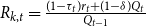 $R_{k,t} = \tfrac {(1-\tau _t)r_t + (1-\delta )Q_t}{Q_{t-1}}$
, where
$R_{k,t} = \tfrac {(1-\tau _t)r_t + (1-\delta )Q_t}{Q_{t-1}}$
, where
 $\tau _t$
is the macroprudential tax. What differs now, however, is that
$\tau _t$
is the macroprudential tax. What differs now, however, is that
 $\tau _2$
affects directly the first intermediation period when the banks’ decisions are forward-looking, and
$\tau _2$
affects directly the first intermediation period when the banks’ decisions are forward-looking, and
 $\tau _3$
the terminal period where the decisions are static. Hence, it follows that
$\tau _3$
the terminal period where the decisions are static. Hence, it follows that
 $\tau _2$
and
$\tau _2$
and
 $\tau _3$
are respectively a forward-looking and a static policy tool.Footnote
36
$\tau _3$
are respectively a forward-looking and a static policy tool.Footnote
36
Analytical welfare effects. We can derive the analytical welfare effects in this case using an analogous procedure based on Davis and Devereux (Reference Davis and Devereux2022). However, a key difference here is that we can track the effect of one more tax, namely, the tool with persistent effects on the balance sheets, which depicts dynamic welfare effects too.
A social planner will consider the following welfare expressions.
 \begin{align*} \begin{split} W_{0}^{a}=u\left (C_{1}^{a}\right ) + \beta u\left (C_{2}^{a}\right ) + \beta ^{2} u\left (C_{3}^{a}\right ) + \lambda _{1}^a\left \{A_{1}^{a} K_{0}^{a \ \alpha }+Q_{1}^{a} I_{1}^{a} - C(I_{1}^{a}, I_{0}^{a}) - \delta _{B} Q_{1}^{a} K_{0}^{a} - C_{1}^{a} - \tfrac {B_{1}^{a}}{R_{1}}\right \} & \\[3pt] +\beta \lambda _{2}^{a}\left \{\varphi (\tau _2^a) A_{2}^{a} K_{1}^{a \ \alpha } + Q_{2}^{a} I_{2}^{a} - C(I_{2}^{a}, I_{1}^{a}) - \delta _{B} Q_{2}^{a} K_{1}^{a}+ \kappa \left (\tfrac {Q_{1}^{a} K_{1}^{a}}{\Lambda _{12}} - \Lambda _{23} \theta Q_{2}^{a} K_{2}^{a}\right ) +B_{1}^{a}-C_{2}^{a} - \tfrac {B_{2}^{a}}{R_{2}}\right \} & \\[3pt] +\beta ^{2} \lambda _{3}^{a}\left \{\left (1-\alpha \left (1-\tau _{3}^{a}\right )\right ) A_{3}^{a} K_{2}^{a \ \alpha }+\kappa \tfrac {Q_{2}^{a} K_{2}^{a}}{\Lambda _{12}}+B_{2}^{a}-C_{3}^{a}\right \}\!,& \end{split} \end{align*}
where
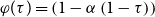 $\varphi (\tau ) = \left (1-\alpha \left (1-\tau \right )\right )$
and with an analogous expression for the economy
$\varphi (\tau ) = \left (1-\alpha \left (1-\tau \right )\right )$
and with an analogous expression for the economy
 $b$
, and
$b$
, and
 \begin{align*} \begin{split} W_{0}^{c}=u\left (C_{1}^{c}\right ) + \beta u\left (C_{2}^{c}\right ) + \beta ^{2} u\left (C_{3}^{c}\right ) +\lambda _{1}^{c}\left \{A_{1}^{c} K_{0}^{c \ \alpha } +Q_{1}^{c} I_{1}^c-C(I_{1}^{c}, I_{0}^{c}) - \delta _{B} Q_{1}^{c} K_{0}^{c} - C_{1}^{c} - \tfrac {B_{1}^{c}}{R_{1}} - D_{1}\right \} &\\[3pt] +\beta \lambda _{2}^{c}\bigg \{ \left (1-\alpha \theta \left (1-\tau _{2}^c\right )\right ) A_{2}^{c} K_{1}^{c \ \alpha }+Q_{2}^{c} I_{2}^{c}-C\left ( I_{2,}^{c} I_{1}^{c}\right ) \bigg . \\[3pt] \left . +(1-\theta )\left ((1-\delta ) Q_{2}^{c} K_{1}^{c}+R_{b 1}^{a} F_{1}^{a}+R_{b 1}^{b} F_{1}^{b}\right ) -\theta R_{1} D_{1} -\delta _{B} Q_{2}^c K_{1}^{c}+B_{1}^{c}-C_{2}^{c}-\tfrac {B_{2}^{c}}{R_{2}}-D_{2} \right \}& \\[3pt] +\beta ^{2} \lambda _{3}^{c}\big \{A_{3}^{c} K_{2}^{c \ \alpha }+(1-\delta ) Q_{3} K_{2}^{c}+R_{b 2}^{a} F_{2}^{a}+R_{b 2}^{b} F_{2}^b+B_{2}-C_{3}^{c}\big \}.& \end{split} \end{align*}
These expressions are obtained by setting the welfare plus the budget constraints in each period and imposing the private equilibrium conditions. These are equivalent to the usual welfare as the constraints are binding; however, this setup allows to gauge the effects of policy more broadly.
As before, we can obtain the welfare effects from changing the taxes. Here, a planner setting the tax in the last period takes the taxes and variables from the previous period as given, and hence, we just need to differentiate with respect to
 $R_2, Q_2, I_2. K_2$
for both types of countries plus
$R_2, Q_2, I_2. K_2$
for both types of countries plus
 $R_{b,2}, F_2$
for the center. In contrast, we must also consider the lagged versions of these variables for the first period.Footnote
37
$R_{b,2}, F_2$
for the center. In contrast, we must also consider the lagged versions of these variables for the first period.Footnote
37
The welfare effects of the taxes are:
For the EMEs’ instruments,
 \begin{equation*} \frac {d W^{a}_0}{d \tau _{2}^{a}}=\beta \lambda _{2}^{a} \bigg \{ \overset {\text{static effects}}{ \overbrace {\alpha _1(\kappa ) \frac {d K_{1}^{a}}{d \tau _{2}^{a}} + \alpha _2(\kappa )\frac {d Q_{1}^{a}}{d \tau _{2}^{a}} + \frac {B_{1}^{a}}{R_{1}} \frac {d R_{1}}{d \tau _{2}^{a}} + \alpha Y_2^a }} + \overset {\text{dynamic effects}}{\overbrace { \alpha _3(\kappa ) \frac {d K_{2}^{a}}{d \tau _{2}^a} + \alpha _4(\kappa ) \frac {d Q_{2}^{a}}{d \tau _{2}^{a}} + \frac {B_{2}^{a}}{(R_{2})^2} \frac {d R_{2}}{d \tau _{2}^{a}} }} \bigg \}, \end{equation*}
 \begin{equation*} \frac {d W^{a}_0}{d \tau _{3}^a}= \left . \beta \lambda _{2}^{a} \bigg \{ \overset { \text{(only) static effects} }{ \overbrace { \alpha _5(\kappa ) \frac {d K_{2}^{a}}{d \tau _{3}^a} + \alpha _4(\kappa ) \frac {d Q_{2}^{a}}{d \tau _{3}^{a}} + \frac {B_{2}^{a}}{(R_{2})^2} \frac {d R_{2}}{d \tau _{3}^{a}} + \alpha \frac {Y_3^a}{R_2} } } \bigg \}, \right . \end{equation*}
with
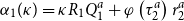 $\alpha _1(\kappa ) = \kappa R_{1} Q_{1}^{a}+\varphi \left (\tau _{2}^{a}\right ) r_2^a$
,
$\alpha _1(\kappa ) = \kappa R_{1} Q_{1}^{a}+\varphi \left (\tau _{2}^{a}\right ) r_2^a$
,
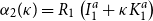 $\alpha _2(\kappa ) = R_1\left (I_{1}^{a}+\kappa K_{1}^{a}\right )$
,
$\alpha _2(\kappa ) = R_1\left (I_{1}^{a}+\kappa K_{1}^{a}\right )$
,
 $\alpha _3(\kappa ) = \kappa \left (1-\theta \Lambda _{23}\right ) Q_{2}^{a} + \varphi \left (\tau _{3}^{a}\right )\Lambda _{12} r_3^a$
,
$\alpha _3(\kappa ) = \kappa \left (1-\theta \Lambda _{23}\right ) Q_{2}^{a} + \varphi \left (\tau _{3}^{a}\right )\Lambda _{12} r_3^a$
,
 $\alpha _4(\kappa ) = I_{2}^{a}+\kappa \left (1-\theta \Lambda _{23}\right )K_{2}^{a}$
,
$\alpha _4(\kappa ) = I_{2}^{a}+\kappa \left (1-\theta \Lambda _{23}\right )K_{2}^{a}$
,
 $\alpha _5(\kappa )=\kappa \left (1-\theta \Lambda _{23}\right ) Q_{2}^{a}+\varphi \left (\tau _{3}^a\right ) \Lambda _{23} r_3^a$
, and
$\alpha _5(\kappa )=\kappa \left (1-\theta \Lambda _{23}\right ) Q_{2}^{a}+\varphi \left (\tau _{3}^a\right ) \Lambda _{23} r_3^a$
, and
 $\tfrac {\partial \alpha _s}{\partial \kappa } \gt 0$
for
$\tfrac {\partial \alpha _s}{\partial \kappa } \gt 0$
for
 $s = \{1, \ldots ,5\}$
.
$s = \{1, \ldots ,5\}$
.
And for the center’s tools,
 \begin{align*} \begin{split} \frac {d W^{c}_0}{d \tau _{2}^c} = \overset {\text{static effects}}{ \overbrace {\beta \lambda _{2}^c \left \{ \gamma _1 \frac {d K_{1}^{c}}{d \tau _{2}^{c}}+\left (\tfrac {B_{1}^{c}}{R_{1}}-\theta D_{1}\right ) \frac {d R_{1}}{d \tau _{2}^{c}} + \tfrac {K_{1}^{c}}{R_1} \frac {d Q_{1}^{c}}{d \tau _{2}^{c}} + \alpha \theta Y_2^c + (1-\theta )\left (F_{1}^{ab} \frac {d R_{b,1}^{eme}}{d \tau _{2}^c} + R_{b,1}^{eme}\frac {d F_{1}^{ab}}{d \tau _{2}^{c}}\right )\right \} }}& \\[3pt] \underset {\text{dynamic effects}}{\underbrace {+\beta ^{2} \lambda _{3}^{c} \left \{ \gamma _2 \frac {d K_{2}^{c}}{d \tau _{2}^{c}} + \tfrac {B_{2}^{c}}{R_{2}} \frac {d R_{2}}{d \tau _{2}^{c}} + \gamma _3 \frac {d Q_{2}^{c}}{d \tau _{2}^{c}} + F_{2}^{ab} \frac {d R_{b,2}^{eme}}{d \tau _{2}^{c}} +R_{b,2}^{eme} \frac {d F_{2}^{ab}}{d \tau _{2}^{c}} \right \}}},& \end{split} \end{align*}
 \begin{align*} \frac {d W^{c}_0}{d \tau _{3}^{c}}=\beta ^{2} \lambda _{3}^{c} \left \{ \gamma _2 \frac {d K_{2}^{c}}{d \tau _{3}^{c}} + \frac {B_{2}^{c}}{R_{2}} \frac {d R_{2}}{d \tau _{3}^{c}} + \gamma _3 \frac {d Q_{2}^{c}}{d \tau _{3}^{c}} + F_{2}^{ab} \frac {d R_{b, 2}^{eme}}{d \tau _{3}^{c}} + R_{b, 2}^{eme}\frac {d F_{2}^{ab}}{d \tau _{3}^{c}} \right \}\!, \end{align*}
with
 $\gamma _1 = \left (1-\alpha \theta \left (1-\tau _{2}^{c}\right )\right ) r_2^c+(1-\theta )(1-\delta ) Q_{2}^{c}$
,
$\gamma _1 = \left (1-\alpha \theta \left (1-\tau _{2}^{c}\right )\right ) r_2^c+(1-\theta )(1-\delta ) Q_{2}^{c}$
,
 $\gamma _2 = \left (r_3^c+(1-\delta ) Q_{3}\right )$
,
$\gamma _2 = \left (r_3^c+(1-\delta ) Q_{3}\right )$
,
 $\gamma _3 = R_2 \big (I_{2}^{c} +(1-\theta ) (1-\delta ) K_{1}^{c}\big )$
, and
$\gamma _3 = R_2 \big (I_{2}^{c} +(1-\theta ) (1-\delta ) K_{1}^{c}\big )$
, and
 $F^{ab}_t = F^a_t + F^b_t$
.
$F^{ab}_t = F^a_t + F^b_t$
.
The interpretation of these effects goes as follows: First, we can see that there are more sources of variations for taxes that are forward-looking in nature (
 $\tau _2$
), whereas for the terminal taxes, we only get the static drivers—described in the simpler baseline; this alone might explain why the former instruments may have stronger welfare effects than the latter.
$\tau _2$
), whereas for the terminal taxes, we only get the static drivers—described in the simpler baseline; this alone might explain why the former instruments may have stronger welfare effects than the latter.
On the other hand, there are four drivers of the static welfare effects of the tax, as pointed out in previous sections: these are changes in welfare from (i) hindering capital accumulation; (ii) changes in the global interest rate, which are proportional to the net foreign asset position; (iii) changes in the prices of capital; and, in addition for the center, (iv) changes in the cross-border lending rates and quantities. The welfare effects (i) and (iv) are negative and capture a halting in banking intermediation, while the sign of (ii) and (iii) depends, respectively, on whether an economy is a net creditor or on the investment growth. We expect (ii) to be positive for an emerging economy and negative for the center.
To reflect on the compared effects relative to our baseline, we can see that the dynamic toolkit effects will have similar drivers but also include effects on future variables, for instance, (i) would include the effect on future capital accumulation and (ii) on the future net assets position. The signs for the dynamic effects may not be as straightforward as we may expect similar signs but with potential corrections, for example, when tighter initial taxes imply delaying investment or capital accumulation plans for future periods. Simultaneously, and similar to the static case, it can be noticed that the welfare effects interact with the extent of the financial frictions (captured by
 $\kappa$
), and, as before, the effects are stronger for a larger extent of the frictions. This can be seen by checking that
$\kappa$
), and, as before, the effects are stronger for a larger extent of the frictions. This can be seen by checking that
 $\alpha _j(\kappa )$
increases in
$\alpha _j(\kappa )$
increases in
 $\kappa$
for all
$\kappa$
for all
 $j = \{1,2,3,4,5\}$
.
$j = \{1,2,3,4,5\}$
.
Optimal taxes. We can obtain expressions for the optimal taxes by taking these welfare effects as first-order conditions for the planner as in prior sections. The features driving each tool are analogous to the ones described in the static baseline. As before, we have that regulators at the center trade-off local intermediation for global lending, a relevant feature for understanding the importance of the center’s instrument in generating cross-border policy leakages and welfare effects abroad. At the same time, and in addition to the previous findings, now we have that the forward-looking taxes are driven by the changes in future variables, for example, capital accumulation after changes in the level of banking intermediation. The expressions for these optimal taxes are shown in Appendix E.
Finally, unlike the static version of the optimal tool, in this case is not as straightforward to determine if a larger extent of the friction calls for a more stringent policy setting. On top of the static amplification effect, the dynamic effect takes into account the expected relative performance of the economy in future periods, which is captured by the interaction between stochastic discount factors on different dates. In that sense, if the friction is such that intermediation implies stronger economic fluctuations (current or future) these additional effects activate.
6. Implications for policy design
We have obtained that there are potentially sizable policy leakages from the prudential policy tool, which depends on how regulation can impact intermediation—mostly at the center but also in peripheral locations. Some of the drivers are related to the capital accumulation, and net foreign assets implications of the resulting capital flows (for all locations) but also to how the toolkit may affect the profits in the banking sector itself (for the center, a global creditor). Importantly, the welfare effects can be magnified if the environment undergoes stronger financial frictions and if the policies are set in an environment of dynamic banking activities where policy-driven changes in contemporaneous profits may remain in the balance sheet of financial agents in the future.
With this in mind, one can also explore what can these policies achieve if they are set optimally. That is, whether they can undo the financial distortions, how similarly are the instruments across different policy regimes—for example, with different degrees of international coordination—and relatedly, whether there is a scope for welfare improvements from centralized regulation setups. We explore these questions by solving for the optimal toolkit of the model.Footnote 38
6.1 Welfare effects in different policy regimes
Before setting the planning problem and solving for the tools, it is useful to understand the welfare effect of the taxes on the policy objective of the planners. For the standard case of a planner that takes decisions at the central level—or a nationally oriented planner—the domestic welfare effect dictates the total effect on her objective function. On the other hand, as we are dealing with several planners, we could also consider that these decide to form coalitions and set their policies with different levels of centralization. The possible combination of cases we consider, the effect of policy changes on their objectives, and the toolkit each planner has at hand are shown in Table 2.
Welfare spillovers in the model
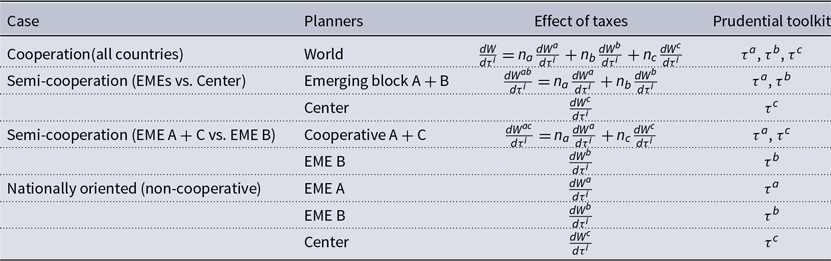
Notes:
 $i$
denotes the country index that also establishes the policy jurisdiction of each tool. For example,
$i$
denotes the country index that also establishes the policy jurisdiction of each tool. For example,
 $\tau ^{i}$
with
$\tau ^{i}$
with
 $i=c$
denotes the policy tool set in country
$i=c$
denotes the policy tool set in country
 $c$
that affects the financial intermediation activities of banks operating in such economy. Additionally, in general,
$c$
that affects the financial intermediation activities of banks operating in such economy. Additionally, in general,
 $i = {a,b,c}$
as the effect on welfare may originate in any economy and affect welfare through their local or international effects.
$i = {a,b,c}$
as the effect on welfare may originate in any economy and affect welfare through their local or international effects.
Table 2 summarizes the effect of any policy change on the objective of each type of planner. To understand the possible effects, we can consider the example of a coalition of two countries, the associated policymakers may decide to cooperate and set their toolkit jointly, and in that case, the policy objective function would be a combination of the welfare of both economies.
With no individual null effects, we have that the total spillover effects between Nash and centralized (or cooperative) cases will differ. As a result, when solving the Ramsey Planning Problems we should obtain different optimal tool levels across policy setups.Footnote 39
The associated Ramsey planner problem is solved for each of the planners in the four cases. This policy problem consists of maximizing a welfare objective subject to the conditions characterizing the private equilibrium of other agents. The objective and problem to solve in each regime are explained in detail in Appendix C. Similar to the private equilibrium case, the numerical solutions reported here are solved nonlinearly, but with a system of equations accounting for the first-order necessary conditions of the involved policymakers in each regime. With this, now we can also solve for the taxes as these are no longer taken as given.
6.2 Implied optimal policies
The results, shown in Table 3, reflect the policy trade-off the planners face: they can implement a tax to undo the financial friction or increase financial intermediation and production by subsidizing the banking sector. In the baseline or nationally oriented case, the emerging planners focus on undoing the friction with a tax. The same is true for the center planner. However, the latter taxes the local banking sector heavily to favor intermediation abroad—where its banks could profit at a higher rate—rather than mitigating the friction, a pattern that aligns with the assumption that the friction is present mostly in peripheral countries, as specified in our baseline setup.Footnote 40
Ramsey-optimal taxes under each policy setup
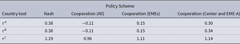
Units: Proportional tax on banking rate of return.
Notes: The solution is obtained using a nonlinear numerical solver of the system of equations characterizing the Ramsey problem allocation of each regime.
When allowing for different levels of cooperation, or of centralization of the policies, we see (from the absolute value of the instruments) that cooperation allows the planner to regulate with more conservative taxes to deliver—as will be shown below—a comparable effect. Interestingly, by internalizing the effect of domestic policies to other locations, a globally cooperative arrangement gives space to subsidize intermediation in emerging economies, while the center taxes are set more loosely which indirectly mitigates the extent of the friction at the peripheries.Footnote 41 Thus, in a fully cooperative case, each country-specific tool is designed with a greater leaning toward generating prosper-thy-neighbor effects. The intuition in this case is that, as long as the frictions are attended in any way (with any country’s toolkit), countries can benefit from higher levels of global intermediation in a similar fashion to how money expansions can be welfare improving for other countries in Obstfeld and Rogoff (Reference Obstfeld and Rogoff1995) and Corsetti and Pesenti (Reference Corsetti and Pesenti2001).
6.3 Effects of policy
We can compare the regimes in terms of other economic outcomes. For example, how effective they are at mitigating the frictions, and the implied welfare they deliver. For that, in Table 4 we show the equivalent compensation changes—in terms of consumption increases—that agents undergo from transitioning from a benchmark allocation to one of the regimes (with optimal policies). For example, if the number is
 $\phi \gt 1$
and the benchmark is the no-policy equilibrium, we say that agents benefit from the policy in a way that would allow them to expand consumption by
$\phi \gt 1$
and the benchmark is the no-policy equilibrium, we say that agents benefit from the policy in a way that would allow them to expand consumption by
 $(\phi -1)\times 100\%$
.Footnote
42
$(\phi -1)\times 100\%$
.Footnote
42
Welfare comparison across policy schemes with respect to the first-best allocation (left panel) and with respect to the no-policy equilibrium (right panel)

Units: Proportional steady-state consumption increase in the benchmark model. That is, by how much consumption in the benchmark should be scaled to match welfare in the column’s regime.
The results indicate that all regimes are capable of mitigating the financial frictions. We can see this in the fact that all countries can improve welfare relative to the no-policy equilibrium. Moreover, they can fully undo the effect of the frictions since the welfare improvement is such that the policies can mimic the first-best allocation (equilibrium in the absence of financial frictions).
A second salient result is that all regimes deliver similar welfare outcomes even if they imply different combinations of prudential tools. This could be deemed surprising given the interpretations provided before. However, this can be the case, as explained by Korinek (Reference Korinek2016), because the conditions for a first-welfare theorem of financial regulations are met. That is, either the cross-border policy spillovers are efficient, the policies are too flexible, or the costs of regulations are trivial. Our setup has at least the two last properties as we don’t constrain the range of possible taxes and the cost of excessive regulation does not affect the policy objective directly.Footnote 43 To explore this we also carry a calculation of the welfare effects in the presence of policy costs in the spirit of Dedola et al. (Reference Dedola, Karadi and Lombardo2013) and Agénor et al. (Reference Agénor, Jackson and Jia2021).
6.4 Policy costs of prudential interventions
To consider the case of costly interventions, we solve the modified Ramsey problems where we include a convex cost of policy implementation. The objective function of the planner becomes
 \begin{gather*} \max _{\mathbf{x_t},\tilde \tau _t} \quad W^{objective}_t = f \big(\alpha ^i,W^i_t\big) {- \Gamma (\tau ^i)}, \\[2pt] s.t. \qquad \mathbb{E}_tF(\mathbf{x_{t-1}}, \mathbf{x_t}, \mathbf{x_{t+1}}, \tau _t, \theta ), \end{gather*}
with
 $ \tilde \tau \subseteq \tau$
and welfare weights
$ \tilde \tau \subseteq \tau$
and welfare weights
 $\alpha ^i \geq 0$
. Here,
$\alpha ^i \geq 0$
. Here,
 $f(\alpha ^i,W^i_t)$
corresponds to the same objective functions considered before and
$f(\alpha ^i,W^i_t)$
corresponds to the same objective functions considered before and
 $\Gamma (\tau ^i) = \psi (\tau ^i)^2$
denotes a quadratic policy implementation cost.Footnote
44
$\Gamma (\tau ^i) = \psi (\tau ^i)^2$
denotes a quadratic policy implementation cost.Footnote
44
The results, reported in Table 5, suggest the presence of gains from policy centralization for every country and globally. In addition, the high cost of policy implementation leads the countries to set their tools much more conservatively compared to the baseline. Finally, every cooperative setup matches the first best.Footnote
45
Put in perspective, these results imply that if regulation is costly, the nationally oriented policies (non-cooperative) can mitigate only about half of the welfare cost of financial frictions that in our baseline amounted to about
 $4\%$
of consumption losses per period. In contrast, the cooperative regimes can bring the economy even closer to the first-best allocation, effectively undoing the remaining welfare cost implied by the friction.
$4\%$
of consumption losses per period. In contrast, the cooperative regimes can bring the economy even closer to the first-best allocation, effectively undoing the remaining welfare cost implied by the friction.
Welfare comparison across policy schemes with respect to the non-cooperative Nash equilibrium and policy implementation costs

Units: Proportional steady-state consumption increase in the baseline non-cooperative regime.
Taking stock, a preliminary view to the regimes’ outcomes may hint we should favor the idea that coordination gains are nil. However, the welfare equivalency result is overturned once we introduce regulatory costs. The prudential regulation costs can be easily rationalized and are subject of recent studies (e.g., Richter et al. Reference Richter, Schularick and Shim2019; Boar et al. Reference Boar, Gambacorta, Lombardo and da Silva2017). Furthermore, the inclusion of these is meaningful in our framework, as the simplifications—finite horizon and perfect foresight—may undermine the welfare cost of volatile regulations. Due to this, a comprehensive welfare accounting of these gains goes beyond the scope of this paper that instead focuses on the analytical and numerical exploration of the prudential leakages. Nonetheless, although only indicative, the presence of gains based on the higher interventionism of decentralized regulations still aligns with the findings of studies (for alternative instruments and environments) such as Davis and Devereux (Reference Davis and Devereux2022), Jin and Shen (Reference Jin and Shen2020), and Agénor et al. (Reference Agénor, Jackson and Jia2021), among others.Footnote 46 , Footnote 47
More importantly for our main research question, the presence of non-trivial policy leakages leads to interdependencies between policymakers in different locations that allow for a wide menu of regulatory combinations to manage the trade-off between undoing financial frictions and curtailing financial intermediation given the costs of regulation. Clearly, and in line with empirical studies, these policies do leak beyond their jurisdiction which can have consequences for policy design adjustments.
7. Conclusions
We study the international policy leakages at the macroprudential level for economies that are financially integrated. The environment we consider is one with a financial center that acts as a global creditor for a set of emerging economies. We aim to verify the existence of these spillovers in different types of economies, their drivers and associated trade-offs, the policies they generate, and the implications for policy design in environments with financial frictions. For that, we propose a multilateral open economy framework in which financial frictions create a wedge between the cost of capital and the deposit rate (or return on non-banking activities) that creates a role for macroprudential interventions. The regulator may want to mitigate the local financial friction by adopting a tighter policy stance, but due to the leakages, the domestic pursuit of financial stability goals may be detrimental to other economies.
Our setup is simplified and allows us to find analytical expressions for the welfare effects of policies and optimal national tools, as well as to obtain numerical solutions for the equilibria in a menu of policy regimes. Our findings suggest that policy spillovers exist and are stronger when stemming from financial centers, but can also originate at emerging economies. Additionally, the effects of the macroprudential toolkit (and leakages) are magnified by the extent of the frictions or in environments involving forward-looking policy decisions.
We inquire into these results and verify that the effects of prudential policymaking are governed by the trade-off between mitigating financial distortions and facilitating financial intermediation. Furthermore, the presence of non-trivial leakages—when internalized—potentially allows regulators to set policies in a prosper-thy-neighbor fashion; in such scenario, emerging economies can set looser financial regulations while financial centers help them deal with the mitigation of financial frictions. Notably, the latter type of economy also benefits from such a strategy given its financial sector acts as a global creditor.
Finally, we explore implications for policy design. In particular, as both the interlinkages and financial distortions may influence the scale and effects of the policy instruments, we compare decentralized (nationally oriented) regimes with alternatives—centralized to a given degree—where countries coordinate their regulations. We find that both can mitigate the financial frictions, but the decentralized regimes must incur in higher interventionism to achieve efficiency. We then consider an extension with explicit costs of interventionism to make the case that leakages may open the scope for internationally coordinated regulations, for which a comprehensive welfare accounting in a stochastic framework beyond our baseline could be carried out. We consider such endeavor a promising venue for future research.
Supplementary material
The supplementary material for this article can be found at https://doi.org/10.1017/S1365100526101047.
Acknowledgments
I thank the feedback and comments of Ippei Fujiwara, Yu-chin Chen, Fabio Ghironi, Galina Hale, Adrian Peralta-Alva, William Barnett, the anonymous referees, and the participants of the Economics Graduate Students Conference (EGSC) 2020 at WUSTL, the 7th workshop on Financial Markets and Non-linear Dynamics (FMND) 2023, the North American Summer Meeting of the Econometric Society 2024, the Society for Economic Measurement 2024 annual meeting, the International Society for the Advancement of Financial Economics 2024 annual meeting, the Midwest Macroeconomics Spring 2025 Meetings, the 2025 RCEA International Conference in Economics, Econometrics, Economics, and Finance, the macroeconomics seminar at Banco de la República, the Phillipps-Universitat Marburg, and at the brown-bag series and workshops at UW Economics. The financial support from the UW Grover and Creta Ensley fellowship is also gratefully acknowledged. Finally, I note that a prior version of this paper circulated with the title: ”Macroprudential Policy Coordination in Open Economies: A Multicountry Framework.”
Competing interests
The author(s) declare none.
Appendix A. Baseline model description and results
A.1 Summary of baseline model equations
The small-scale model after simplifications features 29 variables in total (for the three economies). Each equation ”Common to all countries” enters the system thrice (each with different country variables) for each period indicated. The second group of equations ”for EMEs” enters the system twice (one for each EME country
 $\{a,b\}$
); the rest of equations are counted only once.Footnote
48
$\{a,b\}$
); the rest of equations are counted only once.Footnote
48
Summary of equilibrium equations of the small-scale model

Note: When solving the model, we normalize the initial world capital to 1 and distribute it across countries according to their population sizes. The initial investment is set as
 $I_0 = \delta K_0$
, and an additional simplification is considered (but not substituted) as
$I_0 = \delta K_0$
, and an additional simplification is considered (but not substituted) as
 $R_{k,2}^c = R_{1}$
.
$R_{k,2}^c = R_{1}$
.
Auxiliary definitions:
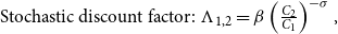 $\text{Stochastic discount factor: } \Lambda _{1,2}=\beta \left (\tfrac {C_{2}}{C_{1}}\right )^{-\sigma },$
 $\text{Lump-sum taxes: }T_{2}=- \tau _{2} r_{2} K_{1},$
 $\text{Marginal product of capital: } r_{2}=\alpha A_{2} K_{1}^{\alpha -1},$
 $\text{Profits of firms: } \pi _{f,t}=(1-\alpha ) A_{t} K_{t-1}^{\alpha }$
, for
$\text{Profits of firms: } \pi _{f,t}=(1-\alpha ) A_{t} K_{t-1}^{\alpha }$
, for
 $t = \{1,2\},$
 $\text{Profits of investors: } \pi _{inv,1} = Q_1I_1 -C(I_1,I_{0}) = Q_{1} I_{1}-I_{1}\left (1+\tfrac {\zeta }{2}\left (\tfrac {I_{1}}{I_{0}}-1\right )^{2}\right ),$
 $\text{Profits of bankers in EMEs, t = 2: } \pi _{b, 2}^{e}=R_{k, 2}^e Q_{1}^{e} K_{1}^{e}-R_{1} F_{1}^{e},$
 $\text{Profits of bankers in the center, t = 2: }\pi _{b,2}^{c}=R_{k,2}^{c} Q_{1}^{c} K_{1}^{c}+R_{1}^{a} F_{1}^{a}+R_{1}^{b} F_{1}^{b}-R_{1} D_{1}.$
Finally, due to the optimality conditions, we can equalize several related rates:
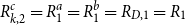 $R_{k,2}^c = R_{1}^a = R_{1}^b = R_{D,1} = R_1$
The system of 29 equations is further simplified as the solution for
$R_{k,2}^c = R_{1}^a = R_{1}^b = R_{D,1} = R_1$
The system of 29 equations is further simplified as the solution for
 $Q_2$
is given by a constant as there is no investment in the final period.Footnote
49
Thus, the final system of equations above consists then on 26 equations (the first panel of equations repeats three times, one for each country, the second twice, one for each emerging country, the third and fourth only appear once) that solve for:
$Q_2$
is given by a constant as there is no investment in the final period.Footnote
49
Thus, the final system of equations above consists then on 26 equations (the first panel of equations repeats three times, one for each country, the second twice, one for each emerging country, the third and fourth only appear once) that solve for:
 $Q_1^a, Q_1^b, Q_1^c, I_1^a, I_1^b, I_1^c, K_1^a, K_1^b, K_1^c, D_1, R_{k,2}^a, R_{k,2}^b, C_1^a, C_1^b, C_1^c, C_2^a, C_2^b, C_2^c, B_1^a, B_1^b, B_1^c, R_1, \mu ^a, \mu ^b, F_1^a, F_1^b$
.
$Q_1^a, Q_1^b, Q_1^c, I_1^a, I_1^b, I_1^c, K_1^a, K_1^b, K_1^c, D_1, R_{k,2}^a, R_{k,2}^b, C_1^a, C_1^b, C_1^c, C_2^a, C_2^b, C_2^c, B_1^a, B_1^b, B_1^c, R_1, \mu ^a, \mu ^b, F_1^a, F_1^b$
.
A.2 Parameters of the models
The table contains the parameters used in the baseline and extended model.
Parameters in the model
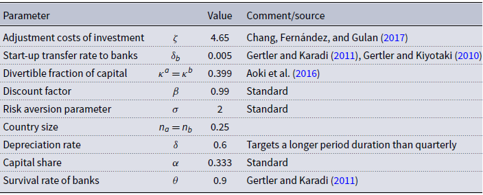
A.3 Data on deposits to GDP
Here we show some data providing support to some of our assumptions and modeling design choices. In particular, we want to support our assumption of a lower financial intermediation capacity and deposits holding in emerging economies (compared to advanced), we do this by showing data of deposits to GDP ratio in a selection of economies that include both developed (advanced) and emerging markets.
Additionally, we show some balance of payments statistics on the international capital outflows to support our claim and focus that the main global creditors are advanced economies and that the typical direction of banking flows is from these economies to emerging markets as depicted in our model.
We can see that the banking (and other capital outflows) originating from advanced economies have a greater scale and volatility, which help motivate our focus on the bilateral flows from financial centers located in these developed economies to other types of economies such as the emerging ones. The flows of this latter type of economies, on the other hand, are not necessarily zero but seem minor in comparison.
Deposits to output ratio in selected economies.
Source: World Bank, Global Financial Development Database (GFDD) 2022.
Note: This figure shows the deposits in the financial system as percentage of GDP (”DI08” in the GFDD database) for a selection of advanced and emerging economies. The dashed lines correspond to the advanced economies.

Capital outflows.
Source: IMF–International Finance Statistics (IFS) database.
Note: The total gross outflows are computed as the sum of foreign direct investment, portfolio, and other (banking) flows. The banking flows correspond to the “other” category. In both cases, we report gross outflows as defined by the IMF: the net acquisition of foreign assets by domestic residents.

A.4 Numerical approximate to the welfare effects in the baseline model
Here we show the approximated numerical derivatives of welfare after changes in the macroprudential instruments in the model.
Policy effects in the model

Note: The effects shown in the table correspond to the numerical approximate to the derivative of welfare with respect to the prudential instrument (
 $\tau$
) in each location. The measure is obtained by solving the model with an increased tax (indicated by the row) and computing the change in the variable relative to the no-taxes (
$\tau$
) in each location. The measure is obtained by solving the model with an increased tax (indicated by the row) and computing the change in the variable relative to the no-taxes (
 $\tau =0$
) equilibrium, and then dividing the resulting number by the change in the tax (
$\tau =0$
) equilibrium, and then dividing the resulting number by the change in the tax (
 $\tfrac {\Delta W}{\Delta \tau }$
). The solution in each case is obtained with a nonlinear solver applied to the equations system in A1. The superindexes refer to the countries with
$\tfrac {\Delta W}{\Delta \tau }$
). The solution in each case is obtained with a nonlinear solver applied to the equations system in A1. The superindexes refer to the countries with
 $a$
: EME-A,
$a$
: EME-A,
 $b$
: EME-B and
$b$
: EME-B and
 $c$
: center. Banking intermediation is measured based on the left-hand side of the balance sheet of the banks, that is,
$c$
: center. Banking intermediation is measured based on the left-hand side of the balance sheet of the banks, that is,
 $L_1^e = Q_1K_1^e$
for EM countries (
$L_1^e = Q_1K_1^e$
for EM countries (
 $e=\{a,b\}$
) and
$e=\{a,b\}$
) and
 $F_1^a + F_1^b + L_1$
for the center. The first column reports the effects for the baseline parameters (Table A2), the second for frictions parameters increased by 25%, and the third for a parameter for country
$F_1^a + F_1^b + L_1$
for the center. The first column reports the effects for the baseline parameters (Table A2), the second for frictions parameters increased by 25%, and the third for a parameter for country
 $a$
increased by 25%.
$a$
increased by 25%.
Appendix B. Analytic welfare effects derivations
This section explains the derivations of the expressions shown in Section 3.
We differentiate the welfare expression for the EME-A social planner:
 \begin{align*} \frac {dW^a}{d \tau ^a} =&\, \lambda _1^a \left [\frac {dQ_1^a}{dI_1^a} I_1^a + Q_1^a - C'\big(I_1^a\big) \right ] \frac {d I_1^a}{d \tau ^a} + \frac {\lambda _1^a}{R_1}\frac {B_1^a}{R_1}\frac {dR_1}{d\tau ^a} \\[2pt] &+ \beta \lambda _2^a \big (\phi (\tau ^a)\alpha A_2^a \xi _2^{a \ \alpha } K_1^{a \ \alpha -1} + \kappa ^a(1-\delta )\xi _2^{a}Q_2\big)\frac {dK_1^a}{d\tau ^a} + \beta \lambda _2^a\alpha (1-\kappa ^a)A_2^a\big(\xi _2^{a} K_1^{a}\big)^\alpha \end{align*}
To obtain the direct welfare effect of the tax we substitute the equilibrium expression for the price of capital for the competitive investor (
 $Q_1^a = C'(I_1^a)$
) and the Euler equation for the consumer (
$Q_1^a = C'(I_1^a)$
) and the Euler equation for the consumer (
 $\lambda _1 = \beta R_1 \lambda _2$
). After rearranging, we obtain the expression shown in the main section:
$\lambda _1 = \beta R_1 \lambda _2$
). After rearranging, we obtain the expression shown in the main section:
 \begin{align*} \frac {dW^a}{d\tau ^a} = \lambda _1^a I_1^a \frac {dQ^a_1}{d\tau ^a} + \beta \lambda _2^a \frac {B^a_1}{R_1} \frac {dR_1}{d\tau ^a} + &\beta \lambda ^a_2 \big ( \phi (\tau ^a) \alpha A_2^a \xi _2^{a \ \alpha } K_1^{a \ \alpha -1} + \kappa ^a(1-\delta )\xi _2^{a}Q_2^a \big ) \frac {dK^a_1}{d\tau ^a} \\[2pt] + &\beta \lambda ^a_2 \alpha (1-\kappa ^a)A^a_2 \big(\xi _2^{a} K_1^{a}\big)^\alpha \end{align*}
The derivation of
 $\frac {dW^b}{d\tau ^b}$
is analogous.
$\frac {dW^b}{d\tau ^b}$
is analogous.
For
 $\frac {dW^c}{d\tau ^c}$
we make the same substitutions for the first two terms and obtain,
$\frac {dW^c}{d\tau ^c}$
we make the same substitutions for the first two terms and obtain,
 \begin{align*} \frac {dW^c}{d\tau ^c} = \lambda _1^c\frac {dQ_1^c}{d\tau ^c}I_1^c + \beta \lambda _2^c \frac {B_1^c}{R_1}\frac {dR_1}{d\tau ^c} + \beta \lambda _2^c \big (\alpha A_2^c \xi _2^{c \ \alpha } K_1^{c \ \alpha -1} + (1-\delta )\xi _2^{c}Q_2 \big)\frac {dK_1^c}{d\tau ^c} \\[2pt]+ \beta \lambda _2^c\left (R_{b,1}^a \frac {dF_1^a}{d\tau ^c} + F_1^a\frac {dR_{b,1}^a}{d\tau ^c} + R_{b,1}^b \frac {dF_1^b}{d\tau ^c} + F_1^b\frac {dR_{b,1}^b}{d\tau ^c}\right ) \end{align*}
In the last term, we use the private equilibrium result:
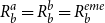 $R_b^a = R_b^b = R_b^{eme}$
 \begin{align*} \frac {dW^c}{d\tau ^c} = \lambda _1^c I_1^c \frac {dQ^c_1}{d\tau ^c} + \beta \lambda _2^c \frac {B^c_1}{R_1} \frac {dR_1}{d\tau ^c} + \beta \lambda _2^c \big (\alpha A_2^c\xi _2^{c \ \alpha }K_1^{c \ \alpha -1} + (1-\delta )\xi _2^{c}Q_2 \big )\frac {dK_1^c}{d\tau ^c} \\[2pt] + \beta \lambda _2 \left [ R_{b,1}^{eme} \left ( \frac {dF_1^a}{d\tau ^c} + \frac {dF_1^b}{d\tau ^c}\right ) + \frac {dR_{b,1}^{eme}}{d\tau ^c} \big ( F_1^a + F_1^b \big )\right ] \end{align*}
We follow the same procedure for the cross-country effects. Notice that the last term of the EME effects will be absent since there is not any direct tax welfare effect at the international level.
To obtain the optimal taxes we set
 $\frac {dW^a}{d\tau ^a} = 0$
and solve for
$\frac {dW^a}{d\tau ^a} = 0$
and solve for
 $\phi (\tau ^a)$
:
$\phi (\tau ^a)$
:
 \begin{equation*} \phi (\tau ^a) = -\frac {1}{\alpha A_2^a \xi _2^{a \ \alpha } K_1^{a \ \alpha -1}}\left [R_1 I_1^a \frac {dQ_1^a}{dK_1^a} + \frac {B_1^a}{R_1}\frac {dR_1}{dK_1^a} + \kappa ^a(1-\delta ) \xi _2^{a} Q_2\right ] \end{equation*}
Where we assumed that
 $\frac {d\tau ^a}{dK_1^a} = 0$
. Assuming taxes exogeneity works here because these calculations are based on the private equilibrium and not on the Ramsey planner equilibrium where the taxes are endogenous.
$\frac {d\tau ^a}{dK_1^a} = 0$
. Assuming taxes exogeneity works here because these calculations are based on the private equilibrium and not on the Ramsey planner equilibrium where the taxes are endogenous.
Now we substitute,
 $\phi (\tau ^a) = 1 + (\kappa ^a - 1)(1 - \tau ^a)\alpha$
and solve for
$\phi (\tau ^a) = 1 + (\kappa ^a - 1)(1 - \tau ^a)\alpha$
and solve for
 $\tau ^a$
:
$\tau ^a$
:
 \begin{equation*} \tau ^{a \ *}{=} -\frac {1}{\alpha (1 - \kappa ^a)} \left \{ \frac {1}{\alpha A^a_2 \xi _2^{a \ \alpha } K_1^{a \ \alpha -1}} \left [ \left ( R_1 I^a_1 \frac {dQ^a_1}{dK^a_1} {+} \frac {B^a_1}{R_1} \frac {dR_1}{dK^a_1} \right ) {+} \kappa ^a (1-\delta )\xi _2^{a}Q_2 \right ] + 1 {+} \alpha (\kappa ^a - 1) \right \} \end{equation*}
The result for
 $b$
is analogous.
$b$
is analogous.
For
 $c$
,
$c$
,
 $\tau ^c$
will not show up in this case because there are not direct tax welfare effects terms for the center. We work around it by using the equilibrium outcome
$\tau ^c$
will not show up in this case because there are not direct tax welfare effects terms for the center. We work around it by using the equilibrium outcome
 $R_{b,1}^{eme} = R_{k,2}^c(\tau ^c)$
. Then we set
$R_{b,1}^{eme} = R_{k,2}^c(\tau ^c)$
. Then we set
 $\frac {dW^c}{d\tau ^c} = 0$
and solve for
$\frac {dW^c}{d\tau ^c} = 0$
and solve for
 $R_{k,2}^c$
:
$R_{k,2}^c$
:
 \begin{equation*} -R_{k,2}^c = R_1I_1\frac {dQ_1^c}{dF^{S}_1} + \frac {B_1^c}{R_1}\frac {dR_1}{dF^S_1} + \big(\alpha A_2^c \xi _2^{c \ \alpha } K_1^{c \ \alpha - 1} + (1-\delta )\xi _2^{c}Q_2 \big) \frac {dK^c_1}{dF^{S}_1} + \big(F_1^a + F_1^b\big)\frac {dR_{b,1}^{eme}}{dF^S_1} \end{equation*}
We substitute
 $R_{k,2}^c = [(1-\tau ^c)\alpha A_2^c\xi _2^{c \ \alpha }K_1^{c \ \alpha -1} + (1-\delta )\xi _2^{c}Q_2]/Q_1^c$
and solve for
$R_{k,2}^c = [(1-\tau ^c)\alpha A_2^c\xi _2^{c \ \alpha }K_1^{c \ \alpha -1} + (1-\delta )\xi _2^{c}Q_2]/Q_1^c$
and solve for
 $\tau ^c$
:
$\tau ^c$
:
 \begin{align*} \tau ^{c \ *} = \frac {Q_1^c}{\alpha A_2^c \xi _2^{c \ \alpha } K_1^{c \ \alpha - 1}} \left \{ R_1 I_1^c \frac {dQ_1^c}{dF^{S}_1} + \frac {B_1^c}{R_1} \frac {dR_1}{dF^{S}_1} + \big(\alpha A_2^c \xi _2^{c \ \alpha } K_1^{c \ \alpha - 1} + (1-\delta )\xi _2^{c}Q_2 \big)\frac {dK^c_1}{dF^{S}_1} \right . \\[2pt] \left . + \, (F_1^a + F_1^b) \frac {dR_{b,1}^{eme}}{dF^{S}_1} + (1 - \delta )\xi _2^{c}\frac {Q_2}{Q_1^c} \right \} + 1 \end{align*}
with
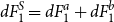 $dF^S_1 = dF_1^a + dF_1^b$
Appendix C. Ramsey policy problems in the baseline model
In the previous sections, we set up a framework to explore the welfare spillovers from setting the macroprudential tools, including the within effect and the effect between economies. The objective was to understand what drives the welfare effect of setting the tools in general and across policy frameworks with different degrees of cooperation between planners.
It should be noted that in such an analysis, there is a substantial endogeneity given that all the equations (on both sides) depend on the taxes. Hence, other than studying the structure of the effects, or the numerical effect at a pre-defined level of the taxes, it is difficult to solve for the actual optimal policy instruments and thus for the policy distorted equilibrium under each regime.
For carrying out such task, it is more convenient to set a Ramsey problem consisting of maximizing a welfare objective function subject to the private equilibrium optimality conditions.
First, we will use the same country-wise welfare definition as before:
 $W^i = u(C_1^i) + \beta u(C_2^i)$
with
$W^i = u(C_1^i) + \beta u(C_2^i)$
with
 $i=\{a,b,c\}$
and
$i=\{a,b,c\}$
and
 $u(C) = \tfrac {C^{1-\sigma }}{1-\sigma }$
.
$u(C) = \tfrac {C^{1-\sigma }}{1-\sigma }$
.
Second, let
 $F(\! \cdot \!)$
be the set of equations representing the optimality constraints of private agents that characterize the private equilibrium,
$F(\! \cdot \!)$
be the set of equations representing the optimality constraints of private agents that characterize the private equilibrium,
 $\mathbf x$
the system of endogenous or decision variables for the agents,
$\mathbf x$
the system of endogenous or decision variables for the agents,
 $\theta$
the parameters of the model and
$\theta$
the parameters of the model and
 $\tau = \{\tau ^a, \tau ^b, \tau ^c \}$
the vector of policy instruments for all countries. In general, we solve the following problem for each Ramsey planner involved:
$\tau = \{\tau ^a, \tau ^b, \tau ^c \}$
the vector of policy instruments for all countries. In general, we solve the following problem for each Ramsey planner involved:
 \begin{gather*} \max _{\mathbf{x_t},\tilde \tau _t} \quad W^{objective}_t = f(\alpha ^i,W^i_t), \\[2pt] s.t. \qquad \mathbb{E}_tF(\mathbf{x_{t-1}}, \mathbf{x_t}, \mathbf{x_{t+1}}, \tau _t, \theta ), \end{gather*}
with
 $ \tilde \tau \subseteq \tau$
and welfare weights
$ \tilde \tau \subseteq \tau$
and welfare weights
 $\alpha ^i \geq 0 \quad \forall i$
.
$\alpha ^i \geq 0 \quad \forall i$
.
The set up of this problem will vary in each policy framework by changing the objective function, whereas the constraints will always refer to all the equations defining the equilibrium of the model (i.e., the system of equations in Table A1). The latter assumption is set for consistency with an open economy setup and implies that the planners acknowledge they have an effect in the endogenous variables of the other countries.Footnote 50
C.1 Non-cooperative framework
Without cooperation we will have one planner for each country, each one solving:
 \begin{align*} &\max _{\mathbf{x^i_t}, \tau ^i_t} \quad W^{i,Nash} = W^i, \\[2pt]& s.t. \quad \mathbb{E}_tF(\mathbf{x_{t-1}}, \mathbf{x_t}, \mathbf{x_{t+1}}, \tau _t, \theta ), \qquad \text{for $t=1$}. \end{align*}
The first-order conditions for the three planners will be used to solve for the Ramsey Nash equilibrium.
C.2 Cooperative frameworks
We will consider three types of cooperative frameworks. Full cooperation, where the tools for all countries are set cooperatively by a single central planner, and two semi-cooperative cases where regional coalitions are formed. First, between emerging economies, and second between the center and one emerging economy. In the semi-cooperative regimes, each coalition will have a central planner setting the participants’ toolkit.
C.2.1 World cooperation
The cooperative Ramsey planner solves:
 \begin{gather*} \max _{\mathbf{x_t}, \tau _t} \quad W^{Coop} = n_a W^a + n_b W^b + n_c W^c, \\[2pt] s.t. \quad \mathbb{E}_tF(\mathbf{x_{t-1}}, \mathbf{x_t}, \mathbf{x_{t+1}}, \tau _t, \theta ), \qquad \text{for $t=1$.} \end{gather*}
Thus, it sets all the tools in order to maximize global (weighted) welfare. The welfare weights correspond to the relative population sizes of the economies.
C.2.2 Regional cooperation between emerging countries
A coalition between emerging economies implies a regional-level planner solving:
 \begin{gather*} \max _{\mathbf{x^a_t}, \mathbf{x^b_t}, \tau ^a_t, \tau ^b_t} \quad W^{Coop,EMEs} = n_a W^a + n_b W^b, \\[2pt] s.t. \quad \mathbb{E}_tF(\mathbf{x_{t-1}}, \mathbf{x_t}, \mathbf{x_{t+1}}, \tau _t, \theta ), \qquad \text{for $t=1$.} \end{gather*}
In this framework, there is a second planner, in the center country, that chooses the decision variables and policy tool for its country in order to maximize
 $W^c_1$
, analogously to the nationally oriented non-cooperative planner.
$W^c_1$
, analogously to the nationally oriented non-cooperative planner.
C.2.3 Coalition between the advanced economy and one emerging country
The coalition between the center (or advanced economy) and one emerging economy (EME-A) implies a semi-cooperative Ramsey planner that solves:
 \begin{gather*} \max _{\mathbf{x^a_t}, \mathbf{x^c_t}, \tau ^a_t, \tau ^c_t} \quad W^{Coop,ac} = n_a W^a + n_c W^c, \\[2pt] s.t. \quad \mathbb{E}_tF(\mathbf{x_{t-1}}, \mathbf{x_t}, \mathbf{x_{t+1}}, \tau _t, \theta ), \qquad \text{for $t=1$.} \end{gather*}
In this case, there is a second planner in the second emerging country (B), that is, the economy outside the coalition, which chooses the B country decision variables and policy tool in order to maximize
 $W^b_1$
, analogously to one of the Nash emerging planners.
$W^b_1$
, analogously to one of the Nash emerging planners.
Appendix D. Numerical simulation results for model extensions
Here we show the additional results for the model with costly policy implementation. In this particular case, the model also depicts frictions in all locations, but as in the baseline, these distortions are considerably more severe in emerging economies and hence, in relative terms, the key modification would be the aversion to policy intervention introduced for the planners.Footnote 51
Welfare comparison for model with frictions in every economy (
 $\kappa ^a = \kappa ^b = 0.399$
and
$\kappa ^a = \kappa ^b = 0.399$
and
 $\kappa ^c = 0.1$
) and policy implementation costs
$\kappa ^c = 0.1$
) and policy implementation costs
 $\psi = 1$

Units: Proportional steady-state consumption increase in the benchmark model.
Ramsey-optimal taxes for the model with frictions in every economy (
 $\kappa ^a = \kappa ^b = 0.399$
and
$\kappa ^a = \kappa ^b = 0.399$
and
 $\kappa ^c = 0.1$
) and policy implementation costs
$\kappa ^c = 0.1$
) and policy implementation costs
 $\psi = 1$

Units: Proportional tax on banking rate of return.
Notes: This case depicts a higher than 100% tax rate on the instrument of country
 $c$
. Although such a tax can be thought of as prohibitive, it should be noted that country
$c$
. Although such a tax can be thought of as prohibitive, it should be noted that country
 $c$
is special in that it derives profits from the intermediation to all locations, and as a consequence, such a tax rate does not have to imply negative profits (as would happen for emerging banks). At the same time, this is a proportional tax on the dividend part of the banking return, so profits can still be large for high values of
$c$
is special in that it derives profits from the intermediation to all locations, and as a consequence, such a tax rate does not have to imply negative profits (as would happen for emerging banks). At the same time, this is a proportional tax on the dividend part of the banking return, so profits can still be large for high values of
 $\tau$
due to the ex-dividend part of the banking return.
$\tau$
due to the ex-dividend part of the banking return.
Appendix E. Results from extended three-period model
E.1 Description of model environment for non-bank agents
Here we discuss the environment for non-bank agents in the context of the environment with multiple periods of intermediation.
E.1.1 Production sectors
There are two types of firms. Here we describe them briefly as the structure is analogous to the main (baseline) model and the detailed formulation is explained in the main document.
Final good firm. There is a firm that maximizes its profits, given by the value of the production, plus the sales of undepreciated capital after production, minus the payment of banking loans. The only constraint it faces is the production technology. From the first-order condition with respect to the capital, we can pin down the gross rate of return paid to the banks as
 $R_{k,t} = \tfrac {r_t + (1-\delta )Q_t}{Q_{t-1}}$
with
$R_{k,t} = \tfrac {r_t + (1-\delta )Q_t}{Q_{t-1}}$
with
 $t=\{2,3\}$
. Here ,
$t=\{2,3\}$
. Here ,
 $r_t = \tfrac {\alpha Y_t}{K_{t-1}}$
is the marginal product of capital.
$r_t = \tfrac {\alpha Y_t}{K_{t-1}}$
is the marginal product of capital.
Capital producers. There is a firm carrying out the investments in each economy. They buy the undepreciated capital from the final good firms and produce the new physical capital for future production. They are subject to adjustment costs relative to the previous investment level.
E.1.2 Households
The households own the three types of firms (final goods, capital, and banks), and use their profits for consumption, saving, and supplying bequests to their banks. They don’t pay the banking taxes directly, instead, these are paid by the banks before distributing profits. However, they receive a lump sum transfer from the government. Since the capital is already predetermined in the initial period, there is no intermediation for
 $K_0$
. Instead, and only for that period, the households rent the capital to the firms directly.
$K_0$
. Instead, and only for that period, the households rent the capital to the firms directly.
EME households. The households maximize the present value of their life-stream of utility:
 \begin{align*} &\max _{ \{C_t^e\}_{t=1}^{3}, \{B_{t}^e\}_{t=1}^{2}} u\big(C_1^e\big) + \beta u\big(C_2^e\big) + \beta ^2 u\big(C_3^e\big), \\[2pt] s.t.\qquad\qquad &\\[2pt] C_1^e + \frac {B_1^e}{R_1^e} &= r_1^e K_0^e + \pi _{f,1}^e + \pi _{inv,1}^e - \delta _B Q_1^e K_0^e, \\[2pt] C_2^e + \frac {B_2^e}{R_2^e} &= \pi _{f,2}^e + \pi _{inv,2}^e + \pi _{bank,2}^e - \delta _B Q_2^e K_1^e + B_1^e - T_2^e, \\[2pt] C_3^e &= \pi _{f,3}^e + \pi _{bank,3}^e + B_2^e - T_3^e, \qquad for \ e = \{a,b\}, \end{align*}
here
 $B_t$
denotes the bonds or net foreign assets position,
$B_t$
denotes the bonds or net foreign assets position,
 $R_t$
the interest rate on bonds, and
$R_t$
the interest rate on bonds, and
 $T_t$
the lump sum taxes. As for the profits terms,
$T_t$
the lump sum taxes. As for the profits terms,
 $\pi _{f,t}$
corresponds to the final goods firms profits,
$\pi _{f,t}$
corresponds to the final goods firms profits,
 $\pi _{inv,t}$
to the capital firms profits, and
$\pi _{inv,t}$
to the capital firms profits, and
 $\pi _{bank,t}$
to the banking profits.
$\pi _{bank,t}$
to the banking profits.
Center households. The households at the center solve a similar problem. The only difference is that they do have access to local deposits and that their banking profits account for the fact that their banks act as creditors of the EMEs:
 \begin{align*} &\max _{ \{C_t^c\}_{t=1}^{3}, \{B_{t}^c\}_{t=1}^{2}} u \big(C_1^c\big) + \beta u\big(C_2^c\big) + \beta ^2 u\big(C_3^c\big), \\[2pt] s.t. \qquad\qquad&\\[-.2cm] C_1^c + \frac {B_1^c}{R_1^c} + D_1 &= r_1^c K_0^c + \pi _{f,1}^c + \pi _{inv,1}^c - \delta _B Q_1^c K_0^c, \\[2pt] C_2^c + \frac {B_2^c}{R_2^c} + D_2 &= \pi _{f,2}^c + \pi _{inv}^c + \pi _{bank,2}^c - \delta _B Q_2^c K_1^c + B_1^c + R_{D,1}D_1 - T_2^c, \\[2pt] C_3^c &= \pi _{f,3}^c + \pi _{bank,3}^c + B_2^c + R_{D,2}D_2 - T_3^c. \end{align*}
E.1.3 Equilibrium
Market clearing and international links. The bonds market depicts a zero-net-supply in the first two periods. The uncovered parity holds, which allows us to equate the interest rate of bonds in each location
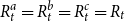 $R_t^a = R_t^b = R_t^c = R_t$
. Furthermore, from the Center’s Euler equations for the deposits and bonds, we can determine that
$R_t^a = R_t^b = R_t^c = R_t$
. Furthermore, from the Center’s Euler equations for the deposits and bonds, we can determine that
 $R_{D,t} = R_t$
for
$R_{D,t} = R_t$
for
 $t = \{1,2\}$
.
$t = \{1,2\}$
.
Equilibrium. Given the policies
 $\tau _t = \{\tau _t^a, \tau _t^b, \tau ^c_t\}_{t=2,3}$
, the equilibrium consists of the prices
$\tau _t = \{\tau _t^a, \tau _t^b, \tau ^c_t\}_{t=2,3}$
, the equilibrium consists of the prices
 $\{Q_t^i\}$
, rates
$\{Q_t^i\}$
, rates
 $\{R_1,R_2,R_{k,2}^i,R_{k,3}^i\}$
and quantities
$\{R_1,R_2,R_{k,2}^i,R_{k,3}^i\}$
and quantities
 $\{B_1^i, B_2^i, K_{1}^i, K_{2}^i, F_1^e,F_2^e,D_1,D_2\}$
and
$\{B_1^i, B_2^i, K_{1}^i, K_{2}^i, F_1^e,F_2^e,D_1,D_2\}$
and
 $\{C_t^i\}$
for
$\{C_t^i\}$
for
 $t = \{1,2,3\}$
, with
$t = \{1,2,3\}$
, with
 $i = \{a,b,c\}$
and
$i = \{a,b,c\}$
and
 $e = \{a,b\}$
such that: in each period, the households solve their utility maximization problem, the firms solve their profit maximization problems, the banks maximize their value, the government runs a balanced budget, and the goods and bonds markets clear.Footnote
52
$e = \{a,b\}$
such that: in each period, the households solve their utility maximization problem, the firms solve their profit maximization problems, the banks maximize their value, the government runs a balanced budget, and the goods and bonds markets clear.Footnote
52
E.2 Final system of equations
Summary of equilibrium equations of the three-period model

Note: When solving the model normalize the initial world capital to 1 and distribute it across countries according to their population sizes. The initial investment is set as
 $I_0 = \delta K_0$
, and since
$I_0 = \delta K_0$
, and since
 $I_3 = 0$
the price
$I_3 = 0$
the price
 $Q_3$
is a constant.
$Q_3$
is a constant.
Auxiliary definitions:
 $\text{Stochastic discount factor: } \Lambda _{t,t+1}=\beta \left (\tfrac {C_{t+1}}{C_{t}}\right )^{-\sigma }$
 $\text{Effective discount factor of banks: } \Omega _{1}=(1-\theta ) \Lambda _{1,2}+\theta ^{2} R_{k, 3} \Lambda _{1,3}$
 $\text{Taxes: }T_{t}=- \tau _{t} r_{t} K_{t-1}$
 $\text{Marginal product of capital: } r_{t}=\alpha A_{t} K_{t-1}^{\alpha -1}$
 $\text{Profits of firms: } \pi _{f,t}=(1-\alpha ) A_{t} K_{t-1}^{\alpha }$
 $\text{Profits of investors: } \pi _{inv,t} = Q_tI_t -C(I_t,I_{t-1}) = Q_{t} I_{t}-I_{t}\left (1+\tfrac {\zeta }{2}\left (\tfrac {I_{t}}{I_{t-1}}-1\right )^{2}\right )$
 $\text{Profits of bankers in EMEs, t = 2: } \pi _{b, 2}^{e}=(1-\theta )\left (R_{k, 2} Q_{1}^{e} K_{1}^{e}-R_{1} F_{1}^{e}\right )$
 $\text{Profits of bankers in EMEs, t = 3: } \pi _{b, 3}^{e}=R_{k, 3}^{e} Q_{2}^{e} K_{2}^{e}-R_{2} F_{2}^{e}, \qquad \text{e = \{a,b\}}$
 $\text{Profits of bankers in Center, t = 2: }\pi _{b,2}^{c}=(1-\theta )\big (R_{k,2}^{c} Q_{1}^{c} K_{1}^{c}+R_{1}^{a} F_{1}^{a}+R_{1}^{b} F_{1}^{b}-R_{1} D_{1}\big )$
 $\text{Profits of bankers in Center, t = 3: }\pi _{b,3}^{c}=R_{k,3}^{c} Q_{2}^{c} K_{2}^{c}+R_{b 2}^{a} F_{2}^{a}+R_{2}^{b} F_{2}^{b}-R_{2} D_{2}$
E.3 Proof of propositions for extended model
Proof of proposition1 for extended model
Proof. W.L.O.G. we will work in a perfect foresight setup, otherwise the same result applies to the expected credit spread.
The time index of the spread is given by the time in which the revenue rate is paid. We can obtain the credit spreads from the EME-Banks F.O.C. with respect to
 $F_1$
and
$F_1$
and
 $F_2$
.
$F_2$
.
For
 $t={2,3}$
the spreads are given by:
$t={2,3}$
the spreads are given by:
 \begin{align*} Spr_2 &= R_{k,2} - R_{b,1} = \frac {\mu _1 \kappa }{(1+\mu _1)\Omega _1} \\[2pt] Spr_3 &= R_{k,3} - R_{b,2} = \frac {\mu _2\kappa }{(1+\mu _2)\Lambda _{2,3}} \end{align*}
if the ICCs bind we have
 $\mu _t \gt 0$
and it follows that:
$\mu _t \gt 0$
and it follows that:
 \begin{align*} \frac {\partial Spr_2}{\partial \kappa } &= \frac {\mu _1}{(1+\mu _1)\Omega _1} \gt 0 \\[2pt] \frac {\partial Spr_3}{\partial \kappa } &= \frac {\mu _2}{(1+\mu _2)\Lambda _{2,3}} \gt 0 \\[-30pt] \end{align*}
Proof of proposition2 for extended model
Proof. W.L.O.G. we will work in a perfect foresight setup, otherwise the same result applies to the expected value of the leverage.
From the ICC of the EME-Banks for each period, we obtain the leverage, defined as total assets over net worth. Then we differentiate the resulting expression with respect to the tax.
For the last period:
The ICC is:
 $J_2 = \Lambda _{2,3}(R_{k,3}L_2 - R_{b,2}F_2) = \kappa _2 L_2$
By substituting the foreign lending
 $F_2 = L_2 - N_2$
, where
$F_2 = L_2 - N_2$
, where
 $N_2$
is the net worth in the last period (bequests plus retained previous profits) and solving for
$N_2$
is the net worth in the last period (bequests plus retained previous profits) and solving for
 $L_2$
:
$L_2$
:
 \begin{equation*} L_2 = \overset {\phi _2}{ \overbrace {\frac {-\Lambda _{2,3}R_{b,2}}{\Lambda _{2,3}(R_{k,3}-R_{b,2}) - \kappa }}}N_2\end{equation*}
where
 $\phi _2$
denotes the leverage. Now, we substitute
$\phi _2$
denotes the leverage. Now, we substitute
 $R_{k,3}(\tau _3) = [(1-\tau _3)r_3 + (1-\delta )Q_3]/Q_2$
and differentiate with respect to the policy instrument:
$R_{k,3}(\tau _3) = [(1-\tau _3)r_3 + (1-\delta )Q_3]/Q_2$
and differentiate with respect to the policy instrument:
 \begin{equation*} \frac {\partial \phi _2}{\partial \tau _3} = -\frac {(\Lambda _{2,3})^2 R_{b,2}\cdot r_3}{(\Lambda _{2,3}(R_{k,3}-R_{b,2}) - \kappa )^2 Q_2} \lt 0 \end{equation*}
For the first period:
The procedure is the same but the algebra is a bit lengthier as we substitute both balance sheets (
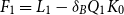 $F_1 = L_1 - \delta _BQ_1K_0$
, and
$F_1 = L_1 - \delta _BQ_1K_0$
, and
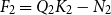 $F_2 = Q_2K_2 - N_2$
) in the value of the bank in the right-hand side of the ICC for the first intermediation period
$F_2 = Q_2K_2 - N_2$
) in the value of the bank in the right-hand side of the ICC for the first intermediation period
 $J_1 = \kappa L_1$
.
$J_1 = \kappa L_1$
.
After substitutions and some algebra, the ICC becomes:
 \begin{equation*} [\tilde \Omega _1 (R_{k,2} - R_{b,1}) - \kappa ]L_1 + [\tilde \Omega _1 R_{b,1}]\delta _BQ_1K_0 + \Lambda _{1,3}\delta [(R_{k,3}-R_{b,2})L_2 + R_{b,2}\delta _BQ_2K_1] = 0 \end{equation*}
With
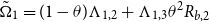 $\tilde \Omega _1 = (1-\theta )\Lambda _{1,2} + \Lambda _{1,3}\theta ^2R_{b,2}$
The leverage is given by:
 \begin{equation*} \phi _1 = \frac {L_1}{\delta _BQ_0K_1} = \frac {-[\tilde \Omega _1 R_{b,1}] - \Lambda _{1,3}\theta [(R_{k,3}-R_{b,2})L_2 + R_{b,2}\delta _BQ_2K_1]/(\delta _BQ_0K_1)}{[\tilde \Omega _1 (R_{k,2} - R_{b,1}) - \kappa ]}\end{equation*}
Then,
 \begin{equation*} \frac {\partial \phi _1}{\partial \tau _2} = - \frac {\tilde \Omega _1 R_{b,1} + \Lambda _{1,3}\theta [(R_{k,3}-R_{b,2})L_2 + R_{b,2}\delta _BQ_2K_1]/(\delta _BQ_0K_1)}{[\tilde \Omega _1 (R_{k,2} - R_{b,1}) - \kappa ]^2}\cdot \left (\frac {r_2(\tau _2)}{Q_1}\right ) \lt 0\end{equation*}
Finally, notice how in the expressions
 $\frac {\partial \phi _1}{\partial \tau _2}$
and
$\frac {\partial \phi _1}{\partial \tau _2}$
and
 $\frac {\partial \phi _2}{\partial \tau _3}$
the denominator implies that the derivatives grow with the friction parameter
$\frac {\partial \phi _2}{\partial \tau _3}$
the denominator implies that the derivatives grow with the friction parameter
 $\kappa$
.
$\kappa$
.
E.4 Optimal taxes in extended model
Individual optimal taxes. The procedure for obtaining the optimal taxes consists of equating the welfare effects
 $\tfrac {dW}{d\tau }$
to zero and then solving for the tax. This is done via backward induction. First, we solve the last period case for
$\tfrac {dW}{d\tau }$
to zero and then solving for the tax. This is done via backward induction. First, we solve the last period case for
 $\tau _3$
, and similarly in the first period for
$\tau _3$
, and similarly in the first period for
 $\tau _2(\tau _3,\cdot )$
. Afterward, we replace the solution found in the first step to obtain
$\tau _2(\tau _3,\cdot )$
. Afterward, we replace the solution found in the first step to obtain
 $\tau _2$
.
$\tau _2$
.
In the case of the center and for the last period, there are no explicit
 $\tau _3^c$
terms in the welfare effect. Then, to pinpoint the tax we use the fact that banking returns show the tax explicitly (
$\tau _3^c$
terms in the welfare effect. Then, to pinpoint the tax we use the fact that banking returns show the tax explicitly (
 $R_{k,3}(\tau _3)$
) to back out the tax after substituting it for one of the rates it equates.
$R_{k,3}(\tau _3)$
) to back out the tax after substituting it for one of the rates it equates.
 \begin{align*} \begin{split} \tau _{2}^{a}= \overset {\text{contemporaneous component}}{\overbrace {\frac {\alpha - 1}{\alpha } -\frac {1}{\alpha r_{2}^{a}}\left \{\left (I_{1}+\kappa K_{1}\right ) \frac {d Q_{1}^{a}}{d K_{1}^{a}}+\frac {B_{1}^{a}}{R_{1}} \frac {d R_{1}}{d K_{1}^{a}} + \kappa R_1 Q_1^a \right .}} \\[2pt] \end{split} \end{align*}
 \begin{align*} \begin{split} \underset {\text{forward-looking component}}{\underbrace {+\left (1-\frac {\Lambda _{1,2}}{\Lambda _{2,3}}\right ) \alpha _{4}(\kappa ) \frac {d Q_{2}^{a}}{d K_{1}^{a}}+ \big (1-\Lambda _{1,2}\big) \frac {B_{2}^{a}}{R_{2}} \frac {d R_{2}}{d K_{1}^{a}}+ \left . \kappa \left (1+\theta \big (\Lambda _{1,2}-\Lambda _{2,3}\big)-\frac {\Lambda _{1,2}}{\Lambda _{2,3}}\right ) Q_{2}^{a} \frac {d K_{2}^{a}}{d K_{1}^{a}}\right \} }} \end{split} \end{align*}
 \begin{equation*} \tau _{3}^a=-\frac {1}{\Lambda _{2,3} \alpha r_{3}^{a} } \left \{ \alpha _4(\kappa ) \frac {d Q_{2}^{a}}{d K_{2}^{a}}+\Lambda _{2,3} \frac {B_{2}^{a}}{R_{2}} \frac {d R_{2}}{d K_{2}^{a}}+\kappa \big (1-\theta \Lambda _{2,3}\big ) Q_{2}^{a} \right \} + 1-\frac {1}{\alpha } \end{equation*}
 \begin{align*} \begin{split} \tau _{2}^{c}=\overset {\text{contemporaneous component}}{\overbrace {-\frac {1}{\theta \alpha r_{2}^{c}}\left \{(1-\theta )(1-\delta ) Q_{2}^{c}+\left (\tfrac {B_{1}^{c}}{R_{1}}-\theta D_{1}\right ) \frac {d R_{1}}{d K_{1}^{c}}+R_{1} K_{1}^{c} \frac {d Q_{1}^{c}}{d K_{1}^{c}}\right . +(1-\theta )\left (\frac {d R_{b,1}^{e m e}}{d K_{1}^{c}}F_{1}^{ab}+R_{b 1}^{e m e}\frac {d F_{1}^{ab}}{d K_{1}^{c}}\right )}} \end{split} \end{align*}
 \begin{align*} \begin{split} \underset {\text{forward looking component}}{\underbrace {+\frac {1}{R_{2}} \left [ \gamma _2 \frac {d K_{2}^c}{d K_{1}^c}+\frac {B_{2}^{c}}{R_{2}} \frac {d R_{2}}{d K_{1}^{c}} + \gamma _3 \frac {d Q_{2}^c}{d K_{1}^c} \left . + \left (\frac {d R_{b 2}^{e m e}}{d K_{1}^{2}}F_{2}^{ab}+R_{b 2}^{e m e}\frac {d F_{2}^{ab}}{d K_{1}^{c}}\right ) \right ] \right \}}}+\frac {\alpha \theta - 1}{\alpha \theta } \end{split} \end{align*}
 \begin{align*} \begin{split} \tau _{3}^{c}=\frac {Q_{2}^{c}}{r_{3}^{c}}\left \{\gamma _2 \frac {d K_{2}^{c}}{d F_{2}^{ab}}+\Lambda _{2,3} B_{2}^{c} \frac {d R_{2}}{d F_{2}^{ab}}+ \gamma _3 \frac {d Q_{2}^{c}}{d F_{2}^{ab}}+\big (F_{2}^{ab}\big) \frac {d R_{b 2}^{\text{eme }}}{d F_{2}^{ab}}\right \} +\frac {(1-\delta ) Q_{3}}{r_{3}^{c}}+1, \end{split} \end{align*}
with
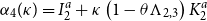 $\alpha _4(\kappa ) = I_{2}^{a}+\kappa \left (1-\theta \Lambda _{2,3}\right ) K_{2}^{a}$
,
$\alpha _4(\kappa ) = I_{2}^{a}+\kappa \left (1-\theta \Lambda _{2,3}\right ) K_{2}^{a}$
,
 $\gamma _2 = r_3^c+(1-\delta ) Q_{3}$
,
$\gamma _2 = r_3^c+(1-\delta ) Q_{3}$
,
 $\gamma _3 = R_2 \left (I_{2}^{c}+(1-\theta )(1-\delta ) K_{1}^{c}\right )$
,
$\gamma _3 = R_2 \left (I_{2}^{c}+(1-\theta )(1-\delta ) K_{1}^{c}\right )$
,
 $F^{ab}_t = F^a_t + F^b_t$
, and
$F^{ab}_t = F^a_t + F^b_t$
, and
 $\tfrac {\partial \alpha _4(\kappa )}{\partial \kappa } \gt 0$
.
$\tfrac {\partial \alpha _4(\kappa )}{\partial \kappa } \gt 0$
.


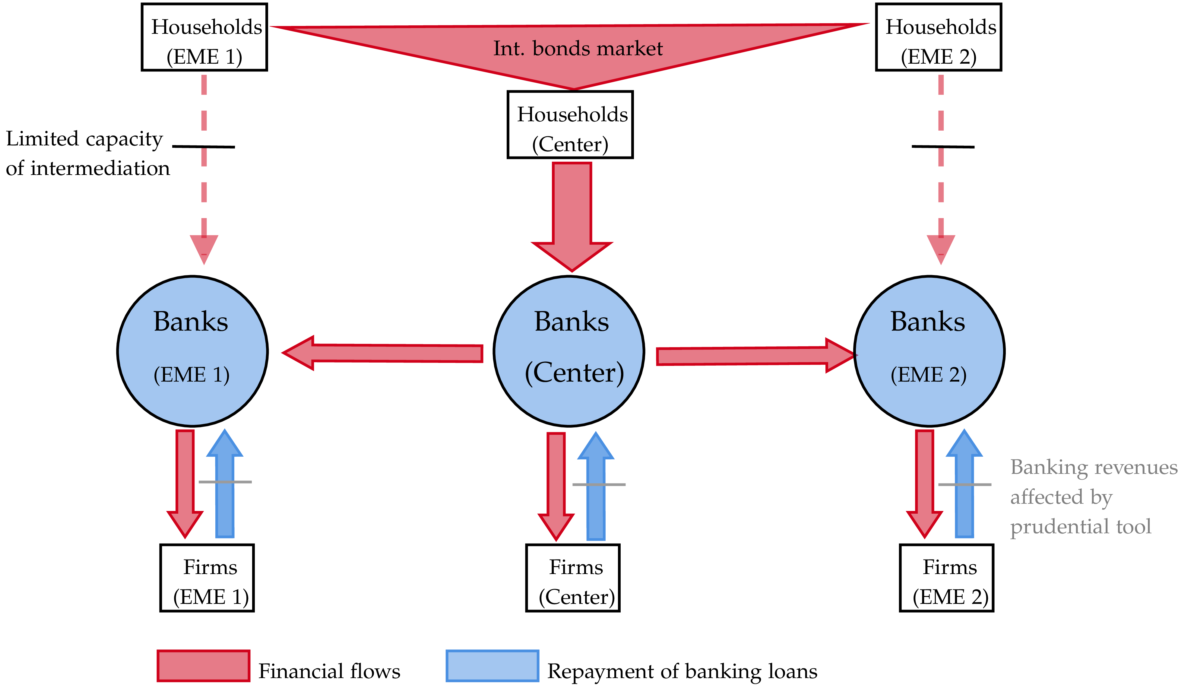


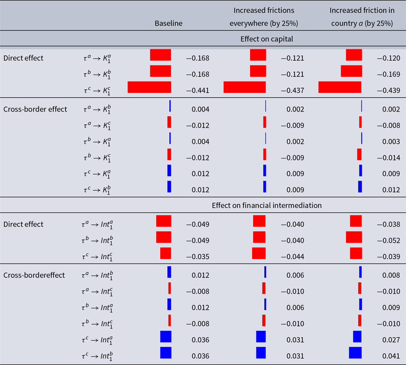


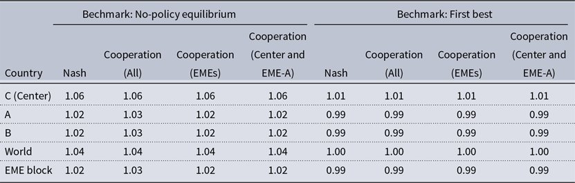
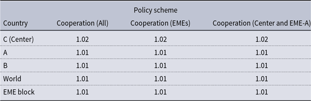
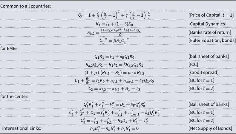

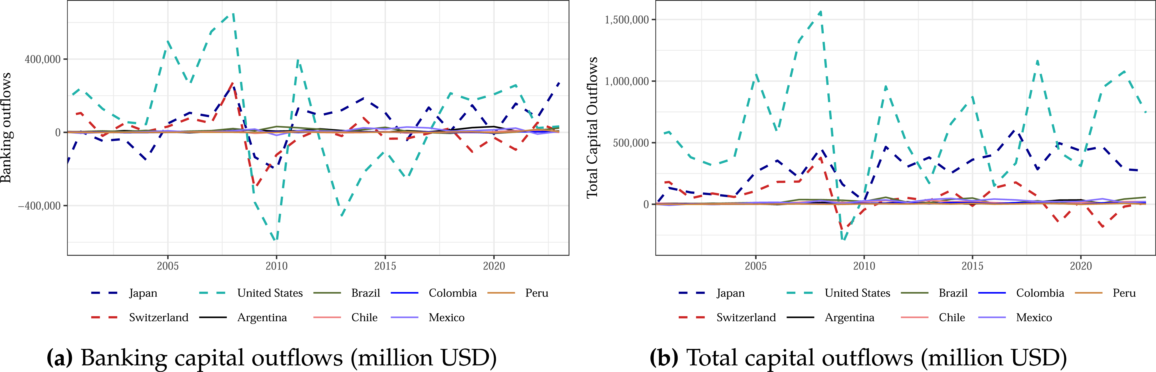
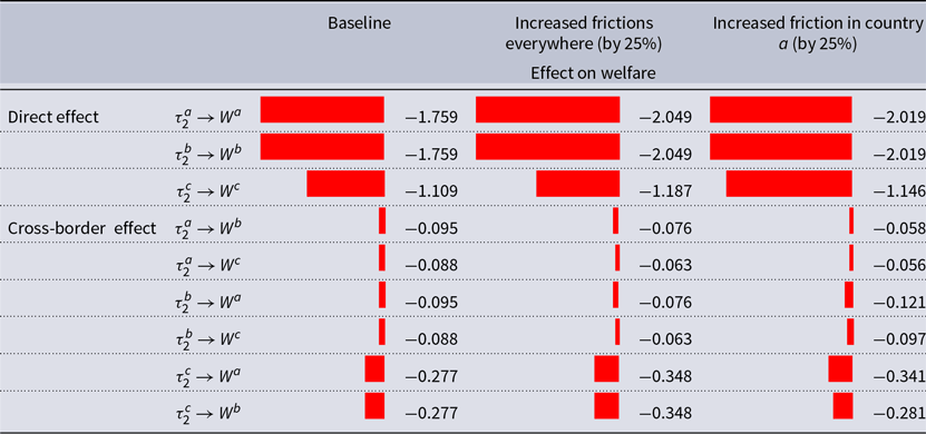
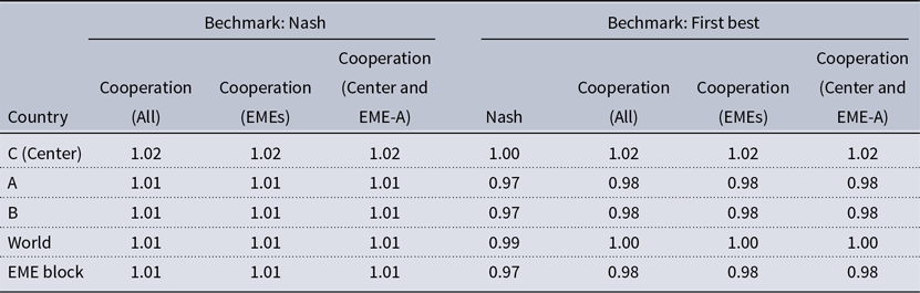


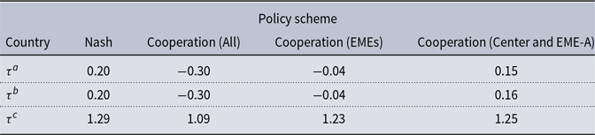


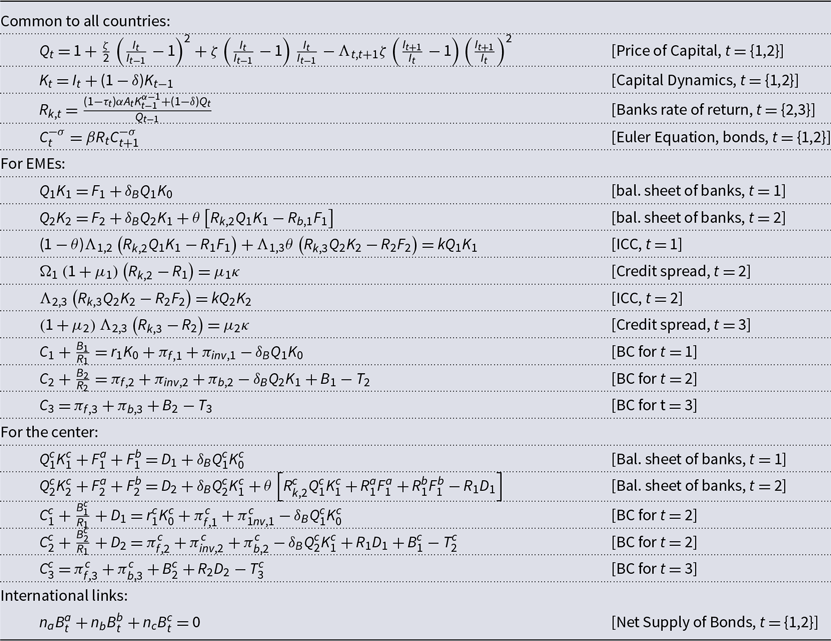


 Open access