


1 Introduction
The chromatic symmetric function $X_G$
of a graph G was introduced by Stanley [Reference Stanley39] as a generalization of Birkhoff’s chromatic polynomial [Reference Birkhoff5]. While the chromatic polynomial enumerates proper graph colorings by the number of colors used,
$X_G$
of a graph G was introduced by Stanley [Reference Stanley39] as a generalization of Birkhoff’s chromatic polynomial [Reference Birkhoff5]. While the chromatic polynomial enumerates proper graph colorings by the number of colors used, $X_G$
also records how many times each color is used. A recent boom of research regarding
$X_G$
also records how many times each color is used. A recent boom of research regarding $X_G$
has focused on the Stanley–Stembridge conjecture [Reference Stanley and Stembridge42], which proposes (in a reformulation by Guay-Paquet [Reference Guay-Paquet17]) that unit interval graphs have chromatic symmetric functions that expand positively in the e-basis of the ring
$X_G$
has focused on the Stanley–Stembridge conjecture [Reference Stanley and Stembridge42], which proposes (in a reformulation by Guay-Paquet [Reference Guay-Paquet17]) that unit interval graphs have chromatic symmetric functions that expand positively in the e-basis of the ring $\mathrm {Sym}$
of symmetric functions. A proof of this conjecture was recently announced by Hikita [Reference Hikita19], by interpreting the coefficients as probabilities.
$\mathrm {Sym}$
of symmetric functions. A proof of this conjecture was recently announced by Hikita [Reference Hikita19], by interpreting the coefficients as probabilities.
To the best of our knowledge, Hikita’s result [Reference Hikita19] does not apply to various generalizations of the chromatic symmetric function and corresponding lifts of the Stanley–Stembridge conjecture, which had been considered both as possible avenues for proving the conjecture and to gain a better understanding of it. Examples of this latter approach include the chromatic quasisymmetric function and Shareshian–Wachs conjecture of [Reference Shareshian and Wachs38] (further studied in [Reference Abreu and Nigro1, Reference Alexandersson and Sulzgruber2, Reference Cho and Hong7, Reference Colmenarejo, Morales and Panova8]), the chromatic nonsymmetric functions of Haglund–Wilson [Reference Haglund and Wilson18] (further studied in [Reference Tewari, Wilson and Zhang43]), and Gebhard–Sagan’s [Reference Gebhard and Sagan16] chromatic symmetric function in noncommuting variables combined with notions of (e)-positivity and appendable (e)-positivity (further studied in [Reference Aliniaeifard, Wang and van Willigenburg3, Reference Dahlberg11, Reference Dahlberg and van Willigenburg13]). Our work provides a novel generalization of $X_G$
in the same vein.
$X_G$
in the same vein.
An important appearance of the ring of symmetric functions $\mathrm {Sym}$
is as the cohomology of complex Grassmannians (parameter spaces for linear subspaces of a vector space) or more precisely for the classifying space
$\mathrm {Sym}$
is as the cohomology of complex Grassmannians (parameter spaces for linear subspaces of a vector space) or more precisely for the classifying space $BU$
. Here, the Schubert classes derived from a natural cell decomposition of
$BU$
. Here, the Schubert classes derived from a natural cell decomposition of $BU$
are represented by the Schur function basis
$BU$
are represented by the Schur function basis $s_\lambda $
of
$s_\lambda $
of $\mathrm {Sym}$
. A richer perspective into the topology of
$\mathrm {Sym}$
. A richer perspective into the topology of $BU$
is obtained by replacing cohomology with a generalized cohomology theory. In particular, there has been much focus on studying the associated combinatorics of the K-theory ring (see [Reference Buch6, Reference Monical, Pechenik and Searles28, Reference Pechenik and Yong32, Reference Thomas and Yong44]). In this context, many of the classical objects of symmetric function theory are seen to have interesting K-analogs, often resembling “superpositions” of classical objects. For example, classical semistandard Young tableaux are replaced by set-valued tableaux (allowing multiple labels per cell), while Schur functions are replaced by Grothendieck polynomials
$BU$
is obtained by replacing cohomology with a generalized cohomology theory. In particular, there has been much focus on studying the associated combinatorics of the K-theory ring (see [Reference Buch6, Reference Monical, Pechenik and Searles28, Reference Pechenik and Yong32, Reference Thomas and Yong44]). In this context, many of the classical objects of symmetric function theory are seen to have interesting K-analogs, often resembling “superpositions” of classical objects. For example, classical semistandard Young tableaux are replaced by set-valued tableaux (allowing multiple labels per cell), while Schur functions are replaced by Grothendieck polynomials $\overline {s}_\lambda $
(inhomogeneous deformations of
$\overline {s}_\lambda $
(inhomogeneous deformations of $s_\lambda $
).
$s_\lambda $
).
Our work introduces a K-analog of the chromatic symmetric function $X_G$
, enumerating colorings of the graph G that assign a nonempty set of distinct colors to each vertex such that adjacent vertices receive disjoint sets. While our Kromatic symmetric function
$X_G$
, enumerating colorings of the graph G that assign a nonempty set of distinct colors to each vertex such that adjacent vertices receive disjoint sets. While our Kromatic symmetric function $\overline {X}_G$
is new, similar functions have been previously considered. The first such functions were originally discussed by Stanley [Reference Stanley40] in the context of graph analogs of symmetric functions, with connections to the real-rootedness of polynomials, and by Gasharov [Reference Gasharov15] in the context of Schur expansions. Recently, as part of his effort to refine Schur-positivity results and the Stanley–Stembridge conjecture, Hwang [Reference Hwang20] studied a similar quasisymmetric function for graphs endowed with a fixed map
$\overline {X}_G$
is new, similar functions have been previously considered. The first such functions were originally discussed by Stanley [Reference Stanley40] in the context of graph analogs of symmetric functions, with connections to the real-rootedness of polynomials, and by Gasharov [Reference Gasharov15] in the context of Schur expansions. Recently, as part of his effort to refine Schur-positivity results and the Stanley–Stembridge conjecture, Hwang [Reference Hwang20] studied a similar quasisymmetric function for graphs endowed with a fixed map $\alpha : V(G) \rightarrow \mathbb {N}$
that dictates the size of the set of colors each vertex receives. To connect chromatic quasisymmetric functions of vertex-weighted graphs to horizontal-strip LLT polynomials, Tom [Reference Tom45] has considered a variant for fixed
$\alpha : V(G) \rightarrow \mathbb {N}$
that dictates the size of the set of colors each vertex receives. To connect chromatic quasisymmetric functions of vertex-weighted graphs to horizontal-strip LLT polynomials, Tom [Reference Tom45] has considered a variant for fixed $\alpha $
with repeated colors allowed. Our work appears to be the first to connect these ideas to the combinatorics of K-theoretic Schubert calculus. (However, [Reference Nenashev and Shapiro29] (see also, [Reference Shapiro, Smirnov and Vaintrob37]) is similar in spirit to our work, developing a K-theoretic analog of the Postnikov–Shapiro algebra [Reference Postnikov and Shapiro36], an apparently unrelated invariant of graphs). After this manuscript appeared in preprint formFootnote
1
, Marberg [Reference Marberg27] gave an interesting Hopf-algebra-theoretic interpretation of
$\alpha $
with repeated colors allowed. Our work appears to be the first to connect these ideas to the combinatorics of K-theoretic Schubert calculus. (However, [Reference Nenashev and Shapiro29] (see also, [Reference Shapiro, Smirnov and Vaintrob37]) is similar in spirit to our work, developing a K-theoretic analog of the Postnikov–Shapiro algebra [Reference Postnikov and Shapiro36], an apparently unrelated invariant of graphs). After this manuscript appeared in preprint formFootnote
1
, Marberg [Reference Marberg27] gave an interesting Hopf-algebra-theoretic interpretation of $\overline {X}_G$
, as well as a quasisymmetric analog from the same perspective.
$\overline {X}_G$
, as well as a quasisymmetric analog from the same perspective.
In this article, having introduced the Kromatic symmetric function, we begin to develop its combinatorial theory. We show that the Kromatic symmetric function $\overline {X}_G$
for any graph G expands positively in a K-theoretic analog (that we also introduce) of the monomial basis of
$\overline {X}_G$
for any graph G expands positively in a K-theoretic analog (that we also introduce) of the monomial basis of $\mathrm {Sym}$
. In this expansion, the coefficients enumerate coverings of the graph by (possibly overlapping) stable sets. We further extend the definition of
$\mathrm {Sym}$
. In this expansion, the coefficients enumerate coverings of the graph by (possibly overlapping) stable sets. We further extend the definition of $\overline {X}_G$
to a vertex-weighted setting, where we give a deletion–contraction relation analogous to that developed by the first and last authors [Reference Crew and Spirkl10] for the vertex-weighted version of
$\overline {X}_G$
to a vertex-weighted setting, where we give a deletion–contraction relation analogous to that developed by the first and last authors [Reference Crew and Spirkl10] for the vertex-weighted version of $X_G$
.
$X_G$
.
Our main result is that the Kromatic symmetric function of a claw-free incomparability graph expands positively in the symmetric Grothendieck basis $\overline {s}_\lambda $
of
$\overline {s}_\lambda $
of $\mathrm {Sym}$
, lifting to K-theory a celebrated result of Gasharov [Reference Gasharov15] that such graphs have Schur-positive chromatic symmetric functions. While all known proofs of Gasharov’s theorem are representation-theoretic or purely combinatorial, the existence of our K-theoretic analog suggests that both results likely also have an interpretation in terms of the topology of Grassmannians. Precisely, for each claw-free incomparability graph G, there should be a subvariety of the Grassmannian whose cohomology class is represented by
$\mathrm {Sym}$
, lifting to K-theory a celebrated result of Gasharov [Reference Gasharov15] that such graphs have Schur-positive chromatic symmetric functions. While all known proofs of Gasharov’s theorem are representation-theoretic or purely combinatorial, the existence of our K-theoretic analog suggests that both results likely also have an interpretation in terms of the topology of Grassmannians. Precisely, for each claw-free incomparability graph G, there should be a subvariety of the Grassmannian whose cohomology class is represented by $X_G$
and whose K-theoretic structure sheaf class is represented by
$X_G$
and whose K-theoretic structure sheaf class is represented by $\overline {X}_G$
. It would be very interesting to have an explicit construction of such subvarieties.
$\overline {X}_G$
. It would be very interesting to have an explicit construction of such subvarieties.
On the other hand, we show that the Kromatic symmetric functions $\overline {X}_{P_n}$
of path graphs
$\overline {X}_{P_n}$
of path graphs $P_n$
generally do not expand positively in either of two K-theoretic deformations we propose for the e-basis of
$P_n$
generally do not expand positively in either of two K-theoretic deformations we propose for the e-basis of $\mathrm {Sym}$
. This fact suggests that the Stanley–Stembridge conjecture is not naturally interpreted in terms of the cohomology of Grassmannians and is unlikely to be amenable to such topological tools from Schubert calculus. (Note that Hikita’s proof [Reference Hikita19] appears to be derived from representation-theoretic considerations, although these are hidden in the actual writeup.) We hope these observations can play a similar role to [Reference Dahlberg, Foley and van Willigenburg12] in limiting the range of potential generalizations of the Stanley–Stembridge conjecture.
$\mathrm {Sym}$
. This fact suggests that the Stanley–Stembridge conjecture is not naturally interpreted in terms of the cohomology of Grassmannians and is unlikely to be amenable to such topological tools from Schubert calculus. (Note that Hikita’s proof [Reference Hikita19] appears to be derived from representation-theoretic considerations, although these are hidden in the actual writeup.) We hope these observations can play a similar role to [Reference Dahlberg, Foley and van Willigenburg12] in limiting the range of potential generalizations of the Stanley–Stembridge conjecture.
This article is organized as follows. In Section 2, we provide an overview of the background and notation used from symmetric function theory (Section 2.1), K-theoretic Schubert calculus (Section 2.2), and graph theory (Section 2.3). In Section 3, we formally introduce the Kromatic symmetric function $\overline {X}_G$
and give its basic properties, including a formula for the expansion in a new K-analog of the monomial basis of
$\overline {X}_G$
and give its basic properties, including a formula for the expansion in a new K-analog of the monomial basis of $\mathrm {Sym}$
and a deletion–contraction relation for a vertex-weighted generalization. We also give our main theorem that the Kromatic symmetric functions of claw-free incomparability graphs expand positively in symmetric Grothendieck functions, lifting the main result of [Reference Gasharov15]. In Section 4, we introduce two different K-theoretic analogs of the e-basis of
$\mathrm {Sym}$
and a deletion–contraction relation for a vertex-weighted generalization. We also give our main theorem that the Kromatic symmetric functions of claw-free incomparability graphs expand positively in symmetric Grothendieck functions, lifting the main result of [Reference Gasharov15]. In Section 4, we introduce two different K-theoretic analogs of the e-basis of $\mathrm {Sym}$
and show that the Kromatic symmetric function
$\mathrm {Sym}$
and show that the Kromatic symmetric function $\overline {X}_{P_3}$
of a
$\overline {X}_{P_3}$
of a $3$
-vertex path graph
$3$
-vertex path graph $P_3$
is not positive in either analog, casting doubt on hopes for a Schubert calculus-based generalization of the Stanley–Stembridge conjecture.
$P_3$
is not positive in either analog, casting doubt on hopes for a Schubert calculus-based generalization of the Stanley–Stembridge conjecture.
2 Background
Throughout this work, $\mathbb {N}$
denotes the set of (strictly) positive integers. We write
$\mathbb {N}$
denotes the set of (strictly) positive integers. We write $[n]$
for the set of positive integers
$[n]$
for the set of positive integers $\{1, 2, \dots , n\}$
. If S is any set,
$\{1, 2, \dots , n\}$
. If S is any set, $2^S$
denotes the power set of all subsets of S.
$2^S$
denotes the power set of all subsets of S.
2.1 Partitions and symmetric functions
In this section, we give a brief overview of the necessary background material. Further details can be found in the textbooks of Stanley [Reference Stanley and Fomin41], Manivel [Reference Manivel26], and Macdonald [Reference Macdonald25].
An ![]() $\lambda = (\lambda _1 \geq \lambda _2 \geq \dots \geq \lambda _k)$
is a finite nonincreasing sequence of positive integers. We define
$\lambda = (\lambda _1 \geq \lambda _2 \geq \dots \geq \lambda _k)$
is a finite nonincreasing sequence of positive integers. We define $\ell (\lambda )$
to be the length of the sequence
$\ell (\lambda )$
to be the length of the sequence $\lambda $
(so above,
$\lambda $
(so above, $\ell (\lambda ) = k$
). We define
$\ell (\lambda ) = k$
). We define $r_i(\lambda )$
to be the number of occurrences of i as a part of
$r_i(\lambda )$
to be the number of occurrences of i as a part of $\lambda $
(so, e.g.,
$\lambda $
(so, e.g., $r_1(2,1,1,1) = 3$
). If
$r_1(2,1,1,1) = 3$
). If
 $$\begin{align*}\sum_{i=1}^{\ell(\lambda)} \lambda_i = n, \end{align*}$$
we say that $\lambda $
is a partition of n, and we write
$\lambda $
is a partition of n, and we write $\lambda \vdash n$
. The
$\lambda \vdash n$
. The ![]() $\lambda $
is a set of squares called
$\lambda $
is a set of squares called ![]() , left- and top-justified (i.e., in “English notation”), such that the ith row from the top contains
, left- and top-justified (i.e., in “English notation”), such that the ith row from the top contains $\lambda _i$
cells. For example, the Young diagram of shape
$\lambda _i$
cells. For example, the Young diagram of shape $(2,2,1)$
is
$(2,2,1)$
is ![]() . Let
. Let $C(\lambda )$
denote the set of cells of the Young diagram of shape
$C(\lambda )$
denote the set of cells of the Young diagram of shape $\lambda $
. If
$\lambda $
. If $\mathsf {c} \in C(\lambda )$
is a cell of the Young diagram of shape
$\mathsf {c} \in C(\lambda )$
is a cell of the Young diagram of shape $\lambda $
, we write
$\lambda $
, we write $\mathsf {c}^\uparrow $
for the cell immediately above
$\mathsf {c}^\uparrow $
for the cell immediately above $\mathsf {c}$
(assuming it exists),
$\mathsf {c}$
(assuming it exists), $\mathsf {c}^\rightarrow $
for the cell immediately right of
$\mathsf {c}^\rightarrow $
for the cell immediately right of $\mathsf {c}$
, and so on. We write
$\mathsf {c}$
, and so on. We write $\lambda ^{\mathsf {T}}$
for the
$\lambda ^{\mathsf {T}}$
for the ![]() of
of $\lambda $
, the integer partition whose Young diagram is obtained from that of
$\lambda $
, the integer partition whose Young diagram is obtained from that of $\lambda $
by exchanging rows and columns.
$\lambda $
by exchanging rows and columns.
Let $S_{\mathbb {N}}$
denote the set of all permutations of the set
$S_{\mathbb {N}}$
denote the set of all permutations of the set $\mathbb {N}$
fixing all but finitely-many elements. A
$\mathbb {N}$
fixing all but finitely-many elements. A ![]()
![]() is a power series of bounded degree such that for each permutation
is a power series of bounded degree such that for each permutation $\sigma \in S_{\mathbb {N}}$
, we have
$\sigma \in S_{\mathbb {N}}$
, we have $f(x_1,x_2,\dots ) = f(x_{\sigma (1)}, x_{\sigma (2)}, \dots )$
. The set
$f(x_1,x_2,\dots ) = f(x_{\sigma (1)}, x_{\sigma (2)}, \dots )$
. The set ![]() of symmetric functions forms a
of symmetric functions forms a $\mathbb {C}$
-vector space. Furthermore, if
$\mathbb {C}$
-vector space. Furthermore, if $\Lambda ^d$
denotes the set of symmetric functions that are homogeneous of degree d, then each
$\Lambda ^d$
denotes the set of symmetric functions that are homogeneous of degree d, then each $\mathrm {Sym}^d$
is a vector space, and
$\mathrm {Sym}^d$
is a vector space, and
 $$\begin{align*}\mathrm{Sym} = \bigoplus_{d=0}^{\infty} \mathrm{Sym}^d \end{align*}$$
as graded vector spaces.
The dimension of $\mathrm {Sym}^d$
as a
$\mathrm {Sym}^d$
as a $\mathbb {C}$
-vector space is equal to the number of integer partitions of d, and many bases of symmetric functions are conveniently indexed by integer partitions. Below, we provide some commonly used bases that will be used in this article.
$\mathbb {C}$
-vector space is equal to the number of integer partitions of d, and many bases of symmetric functions are conveniently indexed by integer partitions. Below, we provide some commonly used bases that will be used in this article.
Definition 2.1 The following are bases of $\mathrm {Sym}$
:
$\mathrm {Sym}$
:
-
• the $\{m_{\lambda }\}$
, defined as where the sum ranges over all distinct monomials formed by choosing distinct positive integers
$$\begin{align*}m_{\lambda} = \sum x_{i_1}^{\lambda_1} \dots x_{i_{\ell(\lambda)}}^{\lambda_{\ell(\lambda)}}, \end{align*}$$
$i_1, \dots , i_{\ell (\lambda )}$
;
$\{m_{\lambda }\}$
, defined as where the sum ranges over all distinct monomials formed by choosing distinct positive integers
$$\begin{align*}m_{\lambda} = \sum x_{i_1}^{\lambda_1} \dots x_{i_{\ell(\lambda)}}^{\lambda_{\ell(\lambda)}}, \end{align*}$$
$i_1, \dots , i_{\ell (\lambda )}$
;
-
• the
$\{ \widetilde {m}_{\lambda } \}$
, defined as
$$\begin{align*}\widetilde{m}_{\lambda} = \left(\prod_{i=1}^{\infty} r_i(\lambda)! \right) m_{\lambda}; \end{align*}$$
-
• the
$\{e_\lambda \}$
, defined by
$$\begin{align*}e_n = \prod_{i_1 < \dots < i_n} x_{i_1} \dots x_{i_n}; \quad e_{\lambda} = e_{\lambda_1} \dots e_{\lambda_{\ell(\lambda)}}; \end{align*}$$
-
• and the
$\{h_\lambda \}$
, defined by
$$\begin{align*}h_n = \prod_{i_1 \leq \dots \leq i_n} x_{i_1} \dots x_{i_n}; \quad h_{\lambda} = h_{\lambda_1} \dots h_{\lambda_{\ell(\lambda)}}. \end{align*}$$


The space of symmetric functions is equipped with a natural inner product $\langle \cdot , \cdot \rangle $
; it may be defined by
$\langle \cdot , \cdot \rangle $
; it may be defined by
 $$\begin{align*}\langle h_{\lambda}, m_{\mu} \rangle = \delta_{\lambda,\mu}, \end{align*}$$
where $\delta _{\bullet , \bullet }$
denotes the Kronecker delta function.
$\delta _{\bullet , \bullet }$
denotes the Kronecker delta function.
We will also need the basis of Schur functions. A ![]() of shape
of shape $\lambda $
is a function
$\lambda $
is a function $T: C(\lambda ) \rightarrow \mathbb {N},$
typically visualized by writing the value
$T: C(\lambda ) \rightarrow \mathbb {N},$
typically visualized by writing the value $T(\mathsf {c})$
in the cell
$T(\mathsf {c})$
in the cell $\mathsf {c}$
. A Young tableau T of shape
$\mathsf {c}$
. A Young tableau T of shape $\lambda $
is
$\lambda $
is ![]() if for each cell
if for each cell $\mathsf {c} \in C(\lambda )$
, we have
$\mathsf {c} \in C(\lambda )$
, we have ${T(\mathsf {c}) \leq T(\mathsf {c}^\rightarrow )}$
and
${T(\mathsf {c}) \leq T(\mathsf {c}^\rightarrow )}$
and $T(\mathsf {c}) < T(\mathsf {c}^\downarrow )$
whenever the cells in question exist. We write
$T(\mathsf {c}) < T(\mathsf {c}^\downarrow )$
whenever the cells in question exist. We write $\mathrm {SSYT}(\lambda )$
for the set of all semistandard Young tableaux of shape
$\mathrm {SSYT}(\lambda )$
for the set of all semistandard Young tableaux of shape $\lambda $
. The
$\lambda $
. The ![]() $s_{\lambda }$
is defined by
$s_{\lambda }$
is defined by
 $$\begin{align*}s_{\lambda} = \sum_{T\in \mathrm{SSYT}(\lambda)} x^T, \quad \text{where} \quad x^T = \prod_{\mathsf{c} \in C(\lambda)} x_{T(\mathsf{c})}.\end{align*}$$
As $\lambda $
ranges over integer partitions, the Schur functions are another basis of
$\lambda $
ranges over integer partitions, the Schur functions are another basis of $\mathrm {Sym}$
. The inner product on
$\mathrm {Sym}$
. The inner product on $\mathrm {Sym}$
also satisfies
$\mathrm {Sym}$
also satisfies
 $$\begin{align*}\langle s_{\lambda}, s_{\mu} \rangle = \delta_{\lambda,\mu}. \end{align*}$$
When $f \in \mathrm {Sym}$
is a symmetric function and
$f \in \mathrm {Sym}$
is a symmetric function and $\{b_{\lambda }\}$
is a basis of symmetric functions indexed by integer partitions
$\{b_{\lambda }\}$
is a basis of symmetric functions indexed by integer partitions $\lambda $
, the notation
$\lambda $
, the notation $[b_{\mu }]f$
denotes the coefficient of
$[b_{\mu }]f$
denotes the coefficient of $b_{\mu }$
when f is expanded in the b-basis. A symmetric function
$b_{\mu }$
when f is expanded in the b-basis. A symmetric function $f \in \mathrm {Sym}$
is said to be
$f \in \mathrm {Sym}$
is said to be ![]() if
if $[b_{\mu }]f$
is nonnegative for every integer partition
$[b_{\mu }]f$
is nonnegative for every integer partition $\mu $
.
$\mu $
.
2.2 K-theoretic Schubert calculus
The ![]() $\Gamma _k = \mathrm {Gr}_k(\mathbb {C}^\infty )$
is the parameter space of k-dimensional vector subspaces of the space of all eventually-zero sequences of complex numbers. The space
$\Gamma _k = \mathrm {Gr}_k(\mathbb {C}^\infty )$
is the parameter space of k-dimensional vector subspaces of the space of all eventually-zero sequences of complex numbers. The space $\Gamma _k$
can be given the structure of a projective Ind-variety and has a cell decomposition into cells
$\Gamma _k$
can be given the structure of a projective Ind-variety and has a cell decomposition into cells $\Gamma _\lambda $
indexed by partitions with at most k parts. Each
$\Gamma _\lambda $
indexed by partitions with at most k parts. Each $\Gamma _\lambda $
induces a cohomology class
$\Gamma _\lambda $
induces a cohomology class $\sigma _\lambda \in H^\star (\Gamma _k)$
and classically we have
$\sigma _\lambda \in H^\star (\Gamma _k)$
and classically we have $H^\star (\Gamma _k) \cong \mathrm {Sym}_k = \mathrm {Sym} \cap \mathbb {C}[x_1, \dots , x_k]$
with the isomorphism taking the class of the cell
$H^\star (\Gamma _k) \cong \mathrm {Sym}_k = \mathrm {Sym} \cap \mathbb {C}[x_1, \dots , x_k]$
with the isomorphism taking the class of the cell $\sigma _\lambda $
to the Schur polynomial
$\sigma _\lambda $
to the Schur polynomial $s_\lambda (x_1, \dots , x_k)$
.
$s_\lambda (x_1, \dots , x_k)$
.
Each cell-closure in $\Gamma _k$
also has a structure sheaf, inducing a class in the representable
$\Gamma _k$
also has a structure sheaf, inducing a class in the representable ![]() ring
ring $K^0(\Gamma _k)$
. These K-theoretic classes are represented by inhomogeneous symmetric polynomials called Grothendieck polynomials
$K^0(\Gamma _k)$
. These K-theoretic classes are represented by inhomogeneous symmetric polynomials called Grothendieck polynomials $\overline {s}_\lambda (x_1, \dots , x_k)$
.
$\overline {s}_\lambda (x_1, \dots , x_k)$
.
A ![]() of shape
of shape $\lambda $
is a filling T of each cell of
$\lambda $
is a filling T of each cell of $C(\lambda )$
with a nonempty set of positive integers. The set-valued tableau T is
$C(\lambda )$
with a nonempty set of positive integers. The set-valued tableau T is ![]() if for each cell
if for each cell ${\mathsf {c} \in C(\lambda )}$
, we have
${\mathsf {c} \in C(\lambda )}$
, we have $\max T(\mathsf {c}) \leq \min T(\mathsf {c}^\rightarrow )$
and
$\max T(\mathsf {c}) \leq \min T(\mathsf {c}^\rightarrow )$
and $\max T(\mathsf {c}) < \min T(\mathsf {c}^\downarrow )$
whenever the cells in question exist. In other words, T is semistandard if every Young tableau formed by choosing one number from the set of each cell is semistandard. For example,
$\max T(\mathsf {c}) < \min T(\mathsf {c}^\downarrow )$
whenever the cells in question exist. In other words, T is semistandard if every Young tableau formed by choosing one number from the set of each cell is semistandard. For example,

is a set-valued tableau of shape $\lambda = (3,2)$
. Let
$\lambda = (3,2)$
. Let $\mathrm {SV}(\lambda )$
denote the set of all semistandard set-valued tableaux of shape
$\mathrm {SV}(\lambda )$
denote the set of all semistandard set-valued tableaux of shape $\lambda $
. The
$\lambda $
. The ![]() $\overline {s}_{\lambda }$
is
$\overline {s}_{\lambda }$
is
 $$\begin{align*}\overline{s}_{\lambda} = \sum_{T \in \mathrm{SV}(\lambda)} (-1)^{|T|-\ell(\lambda)}x^T, \end{align*}$$
where $|T| = \sum _{\mathsf {c} \in C(\lambda )} |T(\mathsf {c})|$
and
$|T| = \sum _{\mathsf {c} \in C(\lambda )} |T(\mathsf {c})|$
and $x^T = \prod _{\mathsf {c} \in C(\lambda )} \prod _{i \in T(\mathsf {c})} x_i$
. Note that
$x^T = \prod _{\mathsf {c} \in C(\lambda )} \prod _{i \in T(\mathsf {c})} x_i$
. Note that $\overline {s}_{\lambda }$
contains terms of degree greater than or equal to
$\overline {s}_{\lambda }$
contains terms of degree greater than or equal to $|\lambda |$
, and that the sum of all of its lowest-degree terms is equal to
$|\lambda |$
, and that the sum of all of its lowest-degree terms is equal to $s_{\lambda }$
. This tableau formula for
$s_{\lambda }$
. This tableau formula for $\overline {s}_\lambda $
is due to Buch [Reference Buch6]. For further background on K-theoretic Schubert calculus and symmetric Grothendieck functions, see [Reference Monical, Pechenik and Searles28, Reference Pechenik and Yong32].
$\overline {s}_\lambda $
is due to Buch [Reference Buch6]. For further background on K-theoretic Schubert calculus and symmetric Grothendieck functions, see [Reference Monical, Pechenik and Searles28, Reference Pechenik and Yong32].
We will also need the ![]() $\underline {s}_\lambda $
defined by
$\underline {s}_\lambda $
defined by
 $$\begin{align*}\langle \overline{s}_{\lambda}, \underline{s}_{\mu} \rangle = \delta_{\lambda,\mu}. \end{align*}$$
Dual symmetric Grothendieck functions were first introduced explicitly in [Reference Lam and Pylyavskyy22] in relation to the K-homology of $\Gamma _k$
; however, they are also implicit in the earlier work [Reference Buch6]. Each
$\Gamma _k$
; however, they are also implicit in the earlier work [Reference Buch6]. Each $\underline {s}_\lambda $
contains terms of degree less than or equal to
$\underline {s}_\lambda $
contains terms of degree less than or equal to $|\lambda |$
; moreover, the sum of all of its highest-degree terms is equal to
$|\lambda |$
; moreover, the sum of all of its highest-degree terms is equal to $s_{\lambda }$
. Although an attractive tableau formula for
$s_{\lambda }$
. Although an attractive tableau formula for $\underline {s}_\lambda $
was given in [Reference Lam and Pylyavskyy22], we do not recall it here, as we will not need it.
$\underline {s}_\lambda $
was given in [Reference Lam and Pylyavskyy22], we do not recall it here, as we will not need it.
2.3 Graphs and coloring
Here, we recall basic notions, terminology, and notations from graph theory. For further details, see the textbooks [Reference Diestel14, Reference West47].
A ![]() G consists of a set V of
G consists of a set V of ![]() , and a set E of unordered pairs of distinct vertices called
, and a set E of unordered pairs of distinct vertices called ![]() . All graphs in this article are simple, so there are no loops and no multi-edges. When
. All graphs in this article are simple, so there are no loops and no multi-edges. When $\{v_1,v_2\} \in E(G)$
, we will typically denote this edge by
$\{v_1,v_2\} \in E(G)$
, we will typically denote this edge by $v_1v_2$
and say
$v_1v_2$
and say $v_1$
and
$v_1$
and $v_2$
are
$v_2$
are ![]() . Two graphs
. Two graphs $G,G'$
are
$G,G'$
are ![]() if there is a bijection
if there is a bijection $\phi : V(G) \to V(G')$
such that, for all vertices
$\phi : V(G) \to V(G')$
such that, for all vertices $v, w \in V(G)$
, we have
$v, w \in V(G)$
, we have $vw \in E(G)$
if and only if
$vw \in E(G)$
if and only if $\phi (v) \phi (w) \in E(G')$
. In this article, we consider graphs up to isomorphism.
$\phi (v) \phi (w) \in E(G')$
. In this article, we consider graphs up to isomorphism.
The ![]() $K_d$
with d vertices is the graph such that
$K_d$
with d vertices is the graph such that $V(K_d) = [d]$
, and
$V(K_d) = [d]$
, and
 $$\begin{align*}E(K_d) = \{vw: v, w \in [d], v \neq w\}.\end{align*}$$
The n-vertex ![]() $P_n$
has vertex set
$P_n$
has vertex set $V(P_n) {\kern-1pt}={\kern-1pt} [n]$
and edge set
$V(P_n) {\kern-1pt}={\kern-1pt} [n]$
and edge set $E(P_n) {\kern-1pt}={\kern-1pt} \{ uv : u,v {\kern-1pt}\in{\kern-1pt} [n], v-u = 1\}$
. The
$E(P_n) {\kern-1pt}={\kern-1pt} \{ uv : u,v {\kern-1pt}\in{\kern-1pt} [n], v-u = 1\}$
. The ![]() $K_{1,3}$
has vertex set
$K_{1,3}$
has vertex set $V(K_{1,3}) = [4]$
and edge set
$V(K_{1,3}) = [4]$
and edge set $E(K_{1,3}) = \{\{1,2\},\{1,3\},\{1,4\}\}$
.
$E(K_{1,3}) = \{\{1,2\},\{1,3\},\{1,4\}\}$
.
An ![]() of a graph G is a graph H such that
of a graph G is a graph H such that $V(H) \subseteq V(G)$
and
$V(H) \subseteq V(G)$
and
 $$\begin{align*}E(H) = \{ vw \in E(G) : v,w \in V(H)\}. \end{align*}$$
We say the graph G is ![]() if no induced subgraph of G is isomorphic to H. We will be especially interested in claw-free graphs.
if no induced subgraph of G is isomorphic to H. We will be especially interested in claw-free graphs.
A ![]() (or
(or ![]() ) of a graph G is a set
) of a graph G is a set $S \subseteq V(G)$
of vertices such that for each
$S \subseteq V(G)$
of vertices such that for each $v, w \in S$
,
$v, w \in S$
, $vw \notin E(G)$
. A
$vw \notin E(G)$
. A ![]() of a graph G is a set
of a graph G is a set $S \subseteq V(G)$
of vertices such that for each
$S \subseteq V(G)$
of vertices such that for each $v \neq w \in S$
,
$v \neq w \in S$
, $vw \in E(G)$
.
$vw \in E(G)$
.
For $\alpha : V(G) \to \mathbb {N}$
a vertex weight function of the graph G, the
$\alpha : V(G) \to \mathbb {N}$
a vertex weight function of the graph G, the $\boldsymbol {\alpha }$
![]() is the graph
is the graph $C_\alpha (G)$
obtained by blowing up each vertex v into a clique of
$C_\alpha (G)$
obtained by blowing up each vertex v into a clique of $\alpha (v)$
vertices. More formally,
$\alpha (v)$
vertices. More formally, $C_\alpha (G)$
has vertex set
$C_\alpha (G)$
has vertex set $ V(C_\alpha (G)) = \{(v,i) : v \in V(G), i \in [\alpha (v)] \}. $
In
$ V(C_\alpha (G)) = \{(v,i) : v \in V(G), i \in [\alpha (v)] \}. $
In $C_\alpha (G)$
, the vertices
$C_\alpha (G)$
, the vertices $(v,i)$
and
$(v,i)$
and $(w,j)$
are adjacent either if
$(w,j)$
are adjacent either if $vw \in E(G)$
or if both
$vw \in E(G)$
or if both $v=w$
and
$v=w$
and $i \neq j$
.
$i \neq j$
.
Given a vertex $v \in V(G)$
, its
$v \in V(G)$
, its ![]() $N(v)$
is defined by
$N(v)$
is defined by $N(v) = \{w: vw \in E(G)\}$
. Given
$N(v) = \{w: vw \in E(G)\}$
. Given $S \subseteq V(G)$
and
$S \subseteq V(G)$
and $v \in V(G)$
with
$v \in V(G)$
with $v \notin S$
, we let
$v \notin S$
, we let $vS \subseteq E(G)$
denote the set of edges
$vS \subseteq E(G)$
denote the set of edges $\{vs: s \in S\}$
. The
$\{vs: s \in S\}$
. The ![]() of a graph G by a pair of distinct vertices
of a graph G by a pair of distinct vertices $v, w \in V(G)$
, denoted
$v, w \in V(G)$
, denoted $G/vw$
, is the graph with vertex set
$G/vw$
, is the graph with vertex set
 $$\begin{align*}V(G/vw) = \left(V(G) \backslash \{v,w\}\right) \cup \{z_{vw}\}, \end{align*}$$
where $z_{vw}$
is a new vertex, and edge set
$z_{vw}$
is a new vertex, and edge set
 $$\begin{align*}E(G/vw) = \left(E(G) \backslash \big( vN(v) \cup wN(w) \big)\right) \cup \big( z_{vw} N(v) \cup z_{vw} N(w) \big). \end{align*}$$
A ![]() of a graph G is a function
of a graph G is a function $\kappa : V(G) \rightarrow \mathbb {N}$
. A coloring
$\kappa : V(G) \rightarrow \mathbb {N}$
. A coloring $\kappa $
of G is
$\kappa $
of G is ![]() if
if $\kappa (a) \neq \kappa (b)$
whenever
$\kappa (a) \neq \kappa (b)$
whenever $ab \in E(G)$
.
$ab \in E(G)$
.
The ![]() [Reference Stanley39] of a graph G is the power series
[Reference Stanley39] of a graph G is the power series
 $$\begin{align*}X_{G} = \sum_{\kappa} \prod_{v \in V(G)} x_{\kappa(v)} \end{align*}$$
where the first sum ranges over all proper colorings $\kappa $
of G. Note that, for every graph G,
$\kappa $
of G. Note that, for every graph G, $X_G \in \mathrm {Sym}$
.
$X_G \in \mathrm {Sym}$
.
2.4 Posets and their incomparability graphs
A ![]() (partially-ordered set)
(partially-ordered set) $(P, \leq )$
is a set P together with a binary relation
$(P, \leq )$
is a set P together with a binary relation $\leq $
that is
$\leq $
that is ![]() (
( $a \leq b$
and
$a \leq b$
and $b \leq c$
implies
$b \leq c$
implies $a \leq c$
),
$a \leq c$
), ![]() (
( $a \leq a$
), and
$a \leq a$
), and ![]() (
( $a\leq b$
and
$a\leq b$
and $b \leq a$
implies
$b \leq a$
implies $a = b$
). For
$a = b$
). For $a,b \in P$
, we write
$a,b \in P$
, we write $a < b$
if
$a < b$
if $a \leq b$
and
$a \leq b$
and $a \neq b$
. We often write P as shorthand for
$a \neq b$
. We often write P as shorthand for $(P, \leq )$
and decorate the relation as
$(P, \leq )$
and decorate the relation as $\leq _P$
for clarity as needed. For more background on posets than is provided here, see [Reference West47].
$\leq _P$
for clarity as needed. For more background on posets than is provided here, see [Reference West47].
When $a,b \in P$
are such that
$a,b \in P$
are such that $a \not \leq b$
and
$a \not \leq b$
and $b \not \leq a$
, we say a and b are
$b \not \leq a$
, we say a and b are ![]() . We write
. We write $\mathbf {n}$
for the unique totally ordered n-element poset and call such a poset a
$\mathbf {n}$
for the unique totally ordered n-element poset and call such a poset a ![]() . The
. The ![]() $P + Q$
of posets
$P + Q$
of posets $(P, \leq _P), (Q, \leq _Q)$
is the disjoint union of sets
$(P, \leq _P), (Q, \leq _Q)$
is the disjoint union of sets $P \sqcup Q$
with the relation
$P \sqcup Q$
with the relation $a \leq _{P+Q} b$
if and only if either
$a \leq _{P+Q} b$
if and only if either $a,b \in P$
with
$a,b \in P$
with $a \leq _P b$
or
$a \leq _P b$
or $a,b \in Q$
with
$a,b \in Q$
with $a \leq _Q b$
.
$a \leq _Q b$
.
We say $(Q, \leq _Q)$
is a
$(Q, \leq _Q)$
is a ![]() of
of $(P, \leq _P)$
if Q is a subset of P and, for all
$(P, \leq _P)$
if Q is a subset of P and, for all $a,b \in Q$
, we have
$a,b \in Q$
, we have $a \leq _Q b$
if and only if
$a \leq _Q b$
if and only if $a \leq _P b$
. Two posets
$a \leq _P b$
. Two posets $(P, \leq _P), (Q, \leq _Q)$
are
$(P, \leq _P), (Q, \leq _Q)$
are ![]() if there is a bijection
if there is a bijection $\phi : P \to Q$
such that, for all
$\phi : P \to Q$
such that, for all $a,b \in P$
, we have
$a,b \in P$
, we have $a \leq _P b$
if and only if
$a \leq _P b$
if and only if $\phi (a) \leq _Q \phi (b)$
. If
$\phi (a) \leq _Q \phi (b)$
. If $(P, \leq _P), (Q, \leq _Q)$
are any two posets, we say that
$(P, \leq _P), (Q, \leq _Q)$
are any two posets, we say that $(P, \leq _P)$
is
$(P, \leq _P)$
is $\boldsymbol {(Q, \leq _Q)}$
![]() if no subposet of P is isomorphic to Q. We will be mostly interested in posets that are
if no subposet of P is isomorphic to Q. We will be mostly interested in posets that are $(\mathbf {3} + \mathbf {1})$
-free.
$(\mathbf {3} + \mathbf {1})$
-free.
Associated with any poset P is its ![]() $I(P)$
. This is the graph whose vertex set is
$I(P)$
. This is the graph whose vertex set is $V(I(P)) = P$
and whose edge set is
$V(I(P)) = P$
and whose edge set is $E(I(P)) = \{ab: a,b \in P, a \not \leq b, b \not \leq a \}$
. That is to say, edges connect incomparable elements of the poset. It is straightforward to see that the poset P is
$E(I(P)) = \{ab: a,b \in P, a \not \leq b, b \not \leq a \}$
. That is to say, edges connect incomparable elements of the poset. It is straightforward to see that the poset P is $(\mathbf {3} + \mathbf {1})$
-free if and only if its incomparability graph is claw-free; however, many claw-free graphs are not incomparability graphs of posets.
$(\mathbf {3} + \mathbf {1})$
-free if and only if its incomparability graph is claw-free; however, many claw-free graphs are not incomparability graphs of posets.
3 The Kromatic symmetric function
3.1 Main definition
A ![]() $(G,\alpha )$
consists of a graph G together with a function
$(G,\alpha )$
consists of a graph G together with a function $\alpha \colon V(G) \rightarrow \mathbb {N}; $
we call
$\alpha \colon V(G) \rightarrow \mathbb {N}; $
we call $\alpha $
the
$\alpha $
the ![]() on the vertices of G. A
on the vertices of G. A ![]() $\boldsymbol {\alpha }$
![]() of G is a function
of G is a function $ \kappa : V(G) \to 2^{\mathbb {N}} \backslash \{\emptyset \} $
assigning to each
$ \kappa : V(G) \to 2^{\mathbb {N}} \backslash \{\emptyset \} $
assigning to each $v \in V(G)$
a set of
$v \in V(G)$
a set of $\alpha (v)$
distinct colors in
$\alpha (v)$
distinct colors in $\mathbb {N}$
, subject to the constraint that when
$\mathbb {N}$
, subject to the constraint that when $uv \in E(G)$
, we have
$uv \in E(G)$
, we have $\kappa (u) \cap \kappa (v) = \emptyset $
. Note that these conditions are equivalent to saying that every choice of a single element from each
$\kappa (u) \cap \kappa (v) = \emptyset $
. Note that these conditions are equivalent to saying that every choice of a single element from each $\kappa (v)$
yields a proper coloring of G. A
$\kappa (v)$
yields a proper coloring of G. A ![]() of G is a proper
of G is a proper $\alpha $
-coloring for some weight function on the vertices of G.
$\alpha $
-coloring for some weight function on the vertices of G.
The ![]() of the vertex-weighted graph
of the vertex-weighted graph $(G,\alpha )$
is
$(G,\alpha )$
is
 $$\begin{align*}X_{G}^\alpha = \sum_{\kappa} \prod_{v \in V(G)} \prod_{i \in \kappa(v)} x_i, \end{align*}$$
where the first sum runs over all proper $\alpha $
-colorings of G. Note that up to a scalar factor depending only on
$\alpha $
-colorings of G. Note that up to a scalar factor depending only on $\alpha $
, the set chromatic symmetric function
$\alpha $
, the set chromatic symmetric function $X_{G}^\alpha $
equals the chromatic symmetric function
$X_{G}^\alpha $
equals the chromatic symmetric function $X_{C_\alpha (G)}$
of the
$X_{C_\alpha (G)}$
of the $\alpha $
-clan graph of G.
$\alpha $
-clan graph of G.
Definition 3.1 The ![]() of a graph G is the symmetric power series
of a graph G is the symmetric power series
 $$\begin{align*}\overline{X}_G = \sum_{\alpha} X_{G}^\alpha, \end{align*}$$
where $\alpha $
ranges over all weight functions of the vertex set
$\alpha $
ranges over all weight functions of the vertex set $V(G)$
.
$V(G)$
.
In other words, $\overline {X}_G$
enumerates all colorings of G by nonempty sets of colors, such that adjacent vertices receive disjoint sets of colors. Note that
$\overline {X}_G$
enumerates all colorings of G by nonempty sets of colors, such that adjacent vertices receive disjoint sets of colors. Note that $\overline {X}_G$
is not a homogeneous symmetric function, but rather consists of
$\overline {X}_G$
is not a homogeneous symmetric function, but rather consists of $X_G$
plus terms of degree higher than
$X_G$
plus terms of degree higher than $|V(G)|$
.
$|V(G)|$
.
Remark 3.2 Stanley [Reference Stanley40] considered a function $Y_G$
related to
$Y_G$
related to $\overline {X}_G$
, although with two differences. Firstly,
$\overline {X}_G$
, although with two differences. Firstly, $Y_G$
uses the rescaled power series
$Y_G$
uses the rescaled power series $X_{C_\alpha (G)}$
in place of
$X_{C_\alpha (G)}$
in place of $X_{G}^\alpha $
. Secondly,
$X_{G}^\alpha $
. Secondly, $Y_G$
allows
$Y_G$
allows $\alpha (v) = 0$
, whereas the Kromatic symmetric function
$\alpha (v) = 0$
, whereas the Kromatic symmetric function $\overline {X}_G$
only considers strictly positive vertex weights. We are unaware of any further study of the functions
$\overline {X}_G$
only considers strictly positive vertex weights. We are unaware of any further study of the functions $Y_G$
since their introduction in [Reference Stanley40].
$Y_G$
since their introduction in [Reference Stanley40].
Remark 3.3 It is easy to observe that the Kromatic symmetric function $\overline {X}_G$
of any graph G is m-positive. Moreover, one may also check that
$\overline {X}_G$
of any graph G is m-positive. Moreover, one may also check that $\overline {X}_G$
is positive in the basis
$\overline {X}_G$
is positive in the basis $\{\omega (p_\lambda )\}_\lambda $
, where
$\{\omega (p_\lambda )\}_\lambda $
, where $p_\lambda $
denotes the power sum symmetric function and
$p_\lambda $
denotes the power sum symmetric function and $\omega $
is the standard involution on symmetric functions.
$\omega $
is the standard involution on symmetric functions.
Although weight functions are used in the definition of $\overline {X}_G$
, the function
$\overline {X}_G$
, the function $\overline {X}_G$
is independent of any particular one. We will find it useful to also consider a vertex-weighted analog of
$\overline {X}_G$
is independent of any particular one. We will find it useful to also consider a vertex-weighted analog of $\overline {X}_G$
. Let
$\overline {X}_G$
. Let $\alpha $
and
$\alpha $
and $\omega $
be independent vertex weight functions on G. Define
$\omega $
be independent vertex weight functions on G. Define
 $$\begin{align*}X_{(G,\omega)}^\alpha = \sum_{\kappa} \prod_{v \in V(G)} \left(\prod_{i \in \kappa(v)} x_i\right)^{\omega(v)}, \end{align*}$$
where again the first sum runs over all proper $\alpha $
-colorings of G. Finally, we define the
$\alpha $
-colorings of G. Finally, we define the ![]() of the vertex-weighted graph
of the vertex-weighted graph $(G,\omega )$
to be
$(G,\omega )$
to be
 $$\begin{align*}\overline{X}_{(G,\omega)} = \sum_{\alpha} X_{(G,\omega)}^\alpha, \end{align*}$$
where the sum is over all weight functions $\alpha $
. In this way,
$\alpha $
. In this way, $\overline {X}_{(G,\omega )}$
is a generating function for proper set colorings of G.
$\overline {X}_{(G,\omega )}$
is a generating function for proper set colorings of G.
3.2 A K-theoretic monomial expansion
For $\lambda $
an integer partition, let
$\lambda $
an integer partition, let $K_\lambda $
denote the vertex-weighted complete graph
$K_\lambda $
denote the vertex-weighted complete graph $(K_{\ell (\lambda )}, \omega )$
, where
$(K_{\ell (\lambda )}, \omega )$
, where $\omega (i) = \lambda _i$
for each i. It is straightforward to see that
$\omega (i) = \lambda _i$
for each i. It is straightforward to see that $X_{K_\lambda } = \widetilde {m}_{\lambda }$
, the augmented monomial symmetric function. Thus, by analogy, we define
$X_{K_\lambda } = \widetilde {m}_{\lambda }$
, the augmented monomial symmetric function. Thus, by analogy, we define
We call $\overline {\widetilde {m}}_{\lambda }$
the
$\overline {\widetilde {m}}_{\lambda }$
the ![]() . To justify this definition, we show that the Kromatic symmetric function of every graph (even every vertex-weighted graph) is a positive sum of K-theoretic augmented monomial symmetric functions.
. To justify this definition, we show that the Kromatic symmetric function of every graph (even every vertex-weighted graph) is a positive sum of K-theoretic augmented monomial symmetric functions.
First, we need some additional definitions. We define a ![]() C of a graph G to be a collection of (distinct) stable sets of G such that every vertex of
C of a graph G to be a collection of (distinct) stable sets of G such that every vertex of $V(G)$
is in at least one element of C. In symbols, this means that
$V(G)$
is in at least one element of C. In symbols, this means that
 $$\begin{align*}\bigcup_{S \in C} S = V(G); \end{align*}$$
note that this union is not required to be disjoint. We write $\mathsf {SSC}(G)$
for the family of all stable set covers of G. For
$\mathsf {SSC}(G)$
for the family of all stable set covers of G. For $C \in \mathsf {SSC}(G)$
, if G is endowed with a vertex weight function
$C \in \mathsf {SSC}(G)$
, if G is endowed with a vertex weight function $\omega $
, let
$\omega $
, let $\lambda (C)$
be the partition of length
$\lambda (C)$
be the partition of length $|C|$
whose parts are
$|C|$
whose parts are $\sum _{v \in S} \omega (v)$
for
$\sum _{v \in S} \omega (v)$
for $S \in C$
. Finally, let the
$S \in C$
. Finally, let the ![]() of the color i in a proper set coloring
of the color i in a proper set coloring $\kappa $
be
$\kappa $
be
 $$\begin{align*}\{v \in V(G) : i \in \kappa(v)\}, \end{align*}$$
the set of vertices of G that receive color i (possibly among other colors) under $\kappa $
.
$\kappa $
.
Proposition 3.4 For any vertex-weighted graph $(G,\omega )$
, we have
$(G,\omega )$
, we have
 $$\begin{align*}\overline{X}_{(G,\omega)} = \sum_{C \in \mathsf{SSC}(G)} \overline{\widetilde{m}}_{\lambda(C)}. \end{align*}$$
Proof The monomials of $\overline {X}_{(G,\omega )}$
correspond to proper set colorings
$\overline {X}_{(G,\omega )}$
correspond to proper set colorings $\kappa $
of G. For each such
$\kappa $
of G. For each such $\kappa $
, note that the set of its color classes is a stable set cover
$\kappa $
, note that the set of its color classes is a stable set cover $C_\kappa $
of G.
$C_\kappa $
of G.
For each $C\in \mathsf {SSC}(G)$
, the monomials of
$C\in \mathsf {SSC}(G)$
, the monomials of $\overline {\widetilde {m}}_{\lambda (C)}$
enumerate all proper set colorings
$\overline {\widetilde {m}}_{\lambda (C)}$
enumerate all proper set colorings $\kappa $
of G such that:
$\kappa $
of G such that:
-
• each
$S \in C$
is the color class of at least one color i under
$\kappa $
, and -
• for each nonempty
$T \subseteq V(G)$
with
$T \notin C$
, there is no color j such that T is the color class of j under
$\kappa $
.


In other words, the monomials of $\overline {\widetilde {m}}_{\lambda (C)}$
correspond to all proper set colorings
$\overline {\widetilde {m}}_{\lambda (C)}$
correspond to all proper set colorings $\kappa $
of G such that
$\kappa $
of G such that $C_\kappa =C$
.
$C_\kappa =C$
.
Since this correspondence between the monomials of $\overline {X}_{(G,\omega )}$
and those of
$\overline {X}_{(G,\omega )}$
and those of $\sum _{C \in \mathsf {SSC}(G)} \overline {\widetilde {m}}_{\lambda (C)}$
is a weight-preserving bijection, the two power series are equal.
$\sum _{C \in \mathsf {SSC}(G)} \overline {\widetilde {m}}_{\lambda (C)}$
is a weight-preserving bijection, the two power series are equal.
We define the ![]() $\overline {p}_\lambda $
to be the Kromatic symmetric function of a disjoint union of vertices with weights
$\overline {p}_\lambda $
to be the Kromatic symmetric function of a disjoint union of vertices with weights $\lambda _1, \dots , \lambda _{\ell (\lambda )}$
. Observe that the ordinary chromatic symmetric function of this graph yields the classical power sum symmetric function
$\lambda _1, \dots , \lambda _{\ell (\lambda )}$
. Observe that the ordinary chromatic symmetric function of this graph yields the classical power sum symmetric function $p_\lambda $
. For some small graphs G, the expansions of
$p_\lambda $
. For some small graphs G, the expansions of $\overline {X}_G$
in the
$\overline {X}_G$
in the $\overline {\widetilde {m}}_{\lambda }$
-basis and the
$\overline {\widetilde {m}}_{\lambda }$
-basis and the $\overline {p}$
-basis are collected in Table 1.
$\overline {p}$
-basis are collected in Table 1.
Kromatic symmetric functions of some small graphs as determined by implementing the deletion–contraction relation of Proposition 3.7 in Python, expressed in the K-theoretic $\overline {\widetilde {m}}$
-basis, as well as in the
$\overline {\widetilde {m}}$
-basis, as well as in the $\overline {p}$
-basis. Since the latter expansion is infinite, we write explicitly only the
$\overline {p}$
-basis. Since the latter expansion is infinite, we write explicitly only the $\overline {p}_\lambda $
with
$\overline {p}_\lambda $
with $|\lambda | \leq |V(G)|+1$
, suppressing higher order terms (“h.o.t.”).
$|\lambda | \leq |V(G)|+1$
, suppressing higher order terms (“h.o.t.”).

Remark 3.5 It is natural to ask if the classical p-basis expansions of $X_G$
lift to
$X_G$
lift to $\overline {p}$
-basis expansions of
$\overline {p}$
-basis expansions of $\overline {X}_G$
. However, it is unclear what this expansion would look like. Attempting to naively modify Stanley’s inclusion–exclusion proof [Reference Stanley39, Theorem 2.5] of this expansion for unweighted graphs fails because it uses the fact that if we take a connected graph G and evaluate
$\overline {X}_G$
. However, it is unclear what this expansion would look like. Attempting to naively modify Stanley’s inclusion–exclusion proof [Reference Stanley39, Theorem 2.5] of this expansion for unweighted graphs fails because it uses the fact that if we take a connected graph G and evaluate $\sum _{\kappa } \prod _{v \in V(G)} x_{\kappa (v)}$
over all
$\sum _{\kappa } \prod _{v \in V(G)} x_{\kappa (v)}$
over all $\kappa $
such that adjacent vertices receive the same color, this yields
$\kappa $
such that adjacent vertices receive the same color, this yields $p_{|V(G)|}$
, since all vertices must have the same color. But in the Kromatic case, the corresponding statement is that color sets of adjacent vertices have nonempty intersection, which yields many possibilities for the corresponding sum over all such colorings. In particular, the result depends on more than just
$p_{|V(G)|}$
, since all vertices must have the same color. But in the Kromatic case, the corresponding statement is that color sets of adjacent vertices have nonempty intersection, which yields many possibilities for the corresponding sum over all such colorings. In particular, the result depends on more than just $|V(G)|$
, making analysis more difficult. It would be interesting to modify this expansion in a way that explains, for example, the data of Table 1. (Since this manuscript first appeared as a preprint, Laura Pierson [Reference Pierson34] has given a complicated formula for the
$|V(G)|$
, making analysis more difficult. It would be interesting to modify this expansion in a way that explains, for example, the data of Table 1. (Since this manuscript first appeared as a preprint, Laura Pierson [Reference Pierson34] has given a complicated formula for the $\overline {p}$
-basis expansion of
$\overline {p}$
-basis expansion of $\overline {X}_G$
, which in particular establishes its integrality.)
$\overline {X}_G$
, which in particular establishes its integrality.)
3.3 A deletion–contraction relation
The Kromatic symmetric function for vertex-weighted graphs also admits a deletion–contraction relation, analogous to that of [Reference Crew and Spirkl10] for the chromatic symmetric function, although somewhat more complicated. We first need to set up some additional notation.
Recall that, given $S \subseteq V(G)$
and
$S \subseteq V(G)$
and $v \in V(G)$
with
$v \in V(G)$
with $v \notin S$
,
$v \notin S$
, $vS$
denotes the set of edges
$vS$
denotes the set of edges $\{vs: s \in S\} \subseteq E(G)$
. Let
$\{vs: s \in S\} \subseteq E(G)$
. Let $(G,\omega )$
be a vertex-weighted graph, and let
$(G,\omega )$
be a vertex-weighted graph, and let $v, w$
be distinct vertices such that
$v, w$
be distinct vertices such that $e = vw \notin E(G)$
. The graph
$e = vw \notin E(G)$
. The graph $G^\star $
has vertex set
$G^\star $
has vertex set
 $$\begin{align*}V(G^\star) = V(G) \cup \{ z^\star\}, \end{align*}$$
where $z^\star $
is a new vertex, and edge set
$z^\star $
is a new vertex, and edge set
 $$\begin{align*}E(G^\star) = E(G) \cup \{vw, vz^\star, wz^\star\} \cup z^\star N(v) \cup z^\star N(w). \end{align*}$$
If G has a vertex weight function $\omega $
, we define an induced vertex weight function
$\omega $
, we define an induced vertex weight function $\omega ^\star $
on
$\omega ^\star $
on $G^\star $
by
$G^\star $
by
 $$\begin{align*}\omega^\star(u) = \begin{cases} \omega(v)+\omega(w), \quad &\text{if}\ u = z^\star;\\ \omega(u), \quad &\text{if}\ u \in V(G). \end{cases} \end{align*}$$
Example 3.6 If G is the tree  , with the leaves being v and w, then $G^\star $
is the complete graph
$G^\star $
is the complete graph  .
.
We also define graphs $G^1, G^2$
with vertex sets
$G^1, G^2$
with vertex sets
 $$\begin{align*}V(G^i) = V(G) \end{align*}$$
and edge sets
 $$\begin{align*}E(G^1) = E(G) \cup e \cup vN(w) \quad \text{and} \quad E(G^2) = E(G) \cup e \cup wN(v). \end{align*}$$
When G has a vertex weight function $\omega $
, there are induced vertex weight functions
$\omega $
, there are induced vertex weight functions $\omega ^i$
on
$\omega ^i$
on $G^i$
given by
$G^i$
given by
 $$\begin{align*}\omega^1(u) = \begin{cases} \omega(v)+\omega(w), \quad &\text{if}\ u = v; \\ \omega(u), \quad &\text{otherwise}; \end{cases} \end{align*}$$
and
 $$\begin{align*}\omega^2(u) = \begin{cases} \omega(v)+\omega(w), \quad &\text{if}\ u = w; \\ \omega(u), \quad &\text{otherwise}. \end{cases} \end{align*}$$
In the contracted graph $G/e$
, we give it the weight function
$G/e$
, we give it the weight function $\omega /e$
defined by
$\omega /e$
defined by
 $$\begin{align*}(\omega/e)(u) = \begin{cases} \omega(v)+\omega(w), \quad &\text{if}\ u = z_{vw}; \\ \omega(u), \quad &\text{otherwise}. \end{cases} \end{align*}$$
Finally, let $G \cup e$
be the graph
$G \cup e$
be the graph $(V(G),E(G)\cup \{e\}$
).
$(V(G),E(G)\cup \{e\}$
).
Proposition 3.7 Let $(G,\omega )$
be a vertex-weighted graph, and let v and w be distinct vertices such that
$(G,\omega )$
be a vertex-weighted graph, and let v and w be distinct vertices such that $e = vw \notin E(G)$
. Then
$e = vw \notin E(G)$
. Then
 $$ \begin{align} \overline{X}_{(G,\omega)} = \overline{X}_{(G / e, \omega / e)}+ \overline{X}_{(G \cup e, \omega)}+ \overline{X}_{(G^1, \omega^1)}+\overline{X}_{(G^2, \omega^2)}+\overline{X}_{(G^\star, \omega^\star)}. \end{align} $$
Proof The proof is a direct bijection between the proper set colorings contributing to the left and right sides of Equation (3.1) as indicated below. In each case, it is straightforward to verify that the given correspondence is reversible, and that the monomials produced by the corresponding colorings are identical.
-
• Proper set colorings
$\kappa $
of
$(G,\omega )$
such that
$\kappa (v) = \kappa (w)$
correspond to all proper set colorings
$\kappa /e$
of
$(G/e,\omega /e)$
by
$$\begin{align*}(\kappa /e)(u) = \begin{cases} \kappa(v), \quad &\text{if}\ u = z_{vw}; \\ \kappa(u), \quad &\text{otherwise}. \end{cases} \end{align*}$$
-
• Proper set colorings
$\kappa $
of
$(G,\omega )$
such that
$\kappa (v) \cap \kappa (w) = \emptyset $
are in exact correspondence with all the proper set colorings of
$(G \cup e, \omega )$
. -
• Proper set colorings
$\kappa $
of
$(G,\omega )$
such that
$\kappa (v) \subsetneq \kappa (w)$
correspond to all proper set colorings
$\kappa ^1$
of
$(G^1, \omega ^1)$
by
$$\begin{align*}\kappa^1(u) = \begin{cases} \kappa(v), \quad &\text{if}\ u=v; \\ \kappa(w)\backslash \kappa(v), \quad &\text{if}\ u=w; \\ \kappa(u), \quad &\text{otherwise}. \end{cases} \end{align*}$$
-
• Proper set colorings
$\kappa $
of
$(G,\omega )$
such that
$\kappa (w) \subsetneq \kappa (v)$
correspond to all proper set colorings
$\kappa ^2$
of
$(G^2, \omega ^2)$
by
$$\begin{align*}\kappa^2(u) = \begin{cases} \kappa(v) \backslash \kappa(w), \quad &\text{if}\ u=v; \\ \kappa(w), \quad &\text{if}\ u=w; \\ \kappa(u), \quad &\text{otherwise}. \end{cases} \end{align*}$$
-
• Proper set colorings
$\kappa $
of
$(G,\omega )$
that fit into none of the previous categories (i.e., those such that each of the sets are nonempty) correspond to all the proper set colorings
$$\begin{align*}\kappa(v) \cap \kappa(w), \kappa(v) \backslash \kappa(w), \kappa(w) \backslash \kappa(v) \end{align*}$$
$\kappa ^\star $
of
$(G^\star ,\omega ^\star )$
by
$$\begin{align*}\kappa^\star(u) = \begin{cases} \kappa(v) \cap \kappa(w), \quad &\text{if}\ u=z^\star; \\ \kappa(v)\backslash \kappa(w), \quad &\text{if}\ u=v; \\ \kappa(w)\backslash \kappa(v), \quad &\text{if}\ u=w; \\ \kappa(u), \quad & \text{otherwise}. \end{cases} \end{align*}$$


This completes the proof of the deletion–contraction relation.
The deletion–contraction relation of Proposition 3.7 can be used to yield algorithmically the $\overline {\widetilde {m}}_\lambda $
-expansion of a Kromatic symmetric function
$\overline {\widetilde {m}}_\lambda $
-expansion of a Kromatic symmetric function $\overline {X}_{(G,\omega )}$
in an alternative fashion to Proposition 3.4. Define the
$\overline {X}_{(G,\omega )}$
in an alternative fashion to Proposition 3.4. Define the ![]() of a graph G to be
of a graph G to be $\operatorname {\mathrm {\mathsf {ts}}}(G) = |\operatorname {\mathrm {\mathsf {SS}}}(G)|-|V(G)|$
, where
$\operatorname {\mathrm {\mathsf {ts}}}(G) = |\operatorname {\mathrm {\mathsf {SS}}}(G)|-|V(G)|$
, where $\operatorname {\mathrm {\mathsf {SS}}}(G)$
denotes the collection of all stable sets of G. Since any single vertex of a graph is a stable set, we may view the total stability as the number of nontrivial stable sets. Thus, note that
$\operatorname {\mathrm {\mathsf {SS}}}(G)$
denotes the collection of all stable sets of G. Since any single vertex of a graph is a stable set, we may view the total stability as the number of nontrivial stable sets. Thus, note that $\operatorname {\mathrm {\mathsf {ts}}}(G) \geq 0$
and that equality holds if and only if G is a complete graph.
$\operatorname {\mathrm {\mathsf {ts}}}(G) \geq 0$
and that equality holds if and only if G is a complete graph.
Corollary 3.8 Recursively applying Proposition 3.7 to a vertex-weighted graph $(G,\omega )$
(iteratively applying it to an arbitrary nonedge of each non-complete graph formed) terminates in a sum of Kromatic symmetric functions of vertex-weighted complete graphs, yielding the
$(G,\omega )$
(iteratively applying it to an arbitrary nonedge of each non-complete graph formed) terminates in a sum of Kromatic symmetric functions of vertex-weighted complete graphs, yielding the $\overline {\widetilde {m}}_{\lambda }$
expansion of
$\overline {\widetilde {m}}_{\lambda }$
expansion of $\overline {X}_{(G,\omega )}$
.
$\overline {X}_{(G,\omega )}$
.
Proof We proceed by induction on the total stability $\operatorname {\mathrm {\mathsf {ts}}}(G)$
. If
$\operatorname {\mathrm {\mathsf {ts}}}(G)$
. If $\operatorname {\mathrm {\mathsf {ts}}}(G) = 0$
, then G is a complete graph and the result is trivial. Otherwise, it is sufficient to show that after applying Proposition 3.7 to
$\operatorname {\mathrm {\mathsf {ts}}}(G) = 0$
, then G is a complete graph and the result is trivial. Otherwise, it is sufficient to show that after applying Proposition 3.7 to $(G,\omega )$
, each of the resulting five graphs
$(G,\omega )$
, each of the resulting five graphs
 $$\begin{align*}G/e, G \cup e, G^1, G^2, G^\star \end{align*}$$
has strictly smaller total stability than G does. We consider each of these five graphs in turn.
-
• (
$\underline{G/e}$
): We have
$|V(G/e)| = |V(G)|-1$
. On the other hand, the stable sets of
$G/e$
not containing
$z_{vw}$
are in obvious bijection with the stable sets of G containing neither v nor w. Moreover, there is a bijection between the stable sets of
$G/e$
containing
$z_{vw}$
and
$\{ S \in \operatorname {\mathrm {\mathsf {SS}}}(G) : v, w\in S\}$
. Together, this gives a bijection between stable sets of
$G/e$
and those stable sets of G which contain either both or neither of v and w. Since
$\{v\}$
and
$\{w\}$
are stable sets of G, we have
$|\operatorname {\mathrm {\mathsf {SS}}}(G/e)| \leq |\operatorname {\mathrm {\mathsf {SS}}}(G)| - 2$
, and so as needed.
$$\begin{align*}\operatorname{\mathrm{\mathsf{ts}}}(G/e) = |\operatorname{\mathrm{\mathsf{SS}}}(G/e)| - |V(G/e)| \leq \big( |\operatorname{\mathrm{\mathsf{SS}}}(G)| - 2 \big) - \big( |V(G)|-1 \big) = \operatorname{\mathrm{\mathsf{ts}}}(G) -1, \end{align*}$$
-
• (
$\underline{G \cup e}$
): We have
$|V(G \cup e)| = |V(G)|$
. Clearly,
$\operatorname {\mathrm {\mathsf {SS}}}(G \cup e) \subseteq \operatorname {\mathrm {\mathsf {SS}}}(G)$
. However, this inclusion is strict since
$\{v,w\} \in \operatorname {\mathrm {\mathsf {SS}}}(G) \backslash \operatorname {\mathrm {\mathsf {SS}}}(G \cup e)$
. Thus,
$\operatorname {\mathrm {\mathsf {ts}}}(G \cup e) < \operatorname {\mathrm {\mathsf {ts}}}(G)$
. -
• (
$\underline{G^1}$
): We have
$|V(G^1)| = |V(G)|$
. Again, it is clear that
$\operatorname {\mathrm {\mathsf {SS}}}(G^1) \subseteq \operatorname {\mathrm {\mathsf {SS}}}(G)$
and the inclusion is strict since
$\{v,w\} \in \operatorname {\mathrm {\mathsf {SS}}}(G) \backslash \operatorname {\mathrm {\mathsf {SS}}}(G^1)$
. -
• (
$\underline{G^2}$
): The analysis is the same as for
$G^1$
. -
• (
$\underline{G^\star} $
): We have
$|V(G^\star )| = |V(G)|+1$
. Let
$X = \{S \in \operatorname {\mathrm {\mathsf {SS}}}(G) : v, w \in S \}$
and let
$Y = \operatorname {\mathrm {\mathsf {SS}}}(G) \backslash X$
. There is an obvious injection of
$\{ S : \operatorname {\mathrm {\mathsf {SS}}}(G^\star ) : z^\star \notin S \}$
into Y, since
$vw \in E(G^\star )$
. We may also biject
$\{ S : \operatorname {\mathrm {\mathsf {SS}}}(G^\star ) : z^\star \in S \}$
with X by mapping
$S \mapsto (S \backslash \{z^\star \}) \cup \{v,w\}$
. This latter map is well-defined since such an S does not include
$v, w$
, or any vertex in
$N(v)$
or
$N(w)$
. Combining these bijections yields a bijection of
$\operatorname {\mathrm {\mathsf {SS}}}(G^\star )$
with
$\operatorname {\mathrm {\mathsf {SS}}}(G)$
, so
$|\operatorname {\mathrm {\mathsf {SS}}}(G^\star )| = |\operatorname {\mathrm {\mathsf {SS}}}(G)|$
. We conclude that
as needed.
$$\begin{align*}\operatorname{\mathrm{\mathsf{ts}}}(G^\star) = |\operatorname{\mathrm{\mathsf{SS}}}(G^\star)| - |V(G^\star)| \leq |\operatorname{\mathrm{\mathsf{SS}}}(G)| - \left( |V(G)|+1 \right) < |\operatorname{\mathrm{\mathsf{SS}}}(G)| - |V(G)| = \operatorname{\mathrm{\mathsf{ts}}}(G), \end{align*}$$


Therefore, the corollary follows by induction on $\operatorname {\mathrm {\mathsf {ts}}}$
.
$\operatorname {\mathrm {\mathsf {ts}}}$
.
3.4 Grothendieck positivity
In 1996, Gasharov [Reference Gasharov15] proved that $X_G$
is Schur-positive for G a claw-free incomparability graph of a poset P by showing that
$X_G$
is Schur-positive for G a claw-free incomparability graph of a poset P by showing that $[s_{\lambda }]X_G$
enumerates objects he called P-tableaux. We now define a generalization of these objects that is enumerated by
$[s_{\lambda }]X_G$
enumerates objects he called P-tableaux. We now define a generalization of these objects that is enumerated by $[\overline {s}_{\lambda }]\overline {X}_G$
. Informally, a Grothendieck P-tableau of shape
$[\overline {s}_{\lambda }]\overline {X}_G$
. Informally, a Grothendieck P-tableau of shape $\lambda $
consists of a P-tableau (as defined in [Reference Gasharov15]) of shape
$\lambda $
consists of a P-tableau (as defined in [Reference Gasharov15]) of shape $\mu $
for some
$\mu $
for some $\mu \subseteq \lambda $
layered with a semistandard Young tableau of shape
$\mu \subseteq \lambda $
layered with a semistandard Young tableau of shape $\lambda /\mu $
that also satisfies “flagging” restrictions on each row. (Similar flagging conditions appear in [Reference Lenart24] with relation to Schur-basis expansions of Grothendieck symmetric functions; we do not know a direct relation between our Grothendieck P-tableaux and [Reference Lenart24], nor with the flagged tableaux of [Reference Wachs46].)
$\lambda /\mu $
that also satisfies “flagging” restrictions on each row. (Similar flagging conditions appear in [Reference Lenart24] with relation to Schur-basis expansions of Grothendieck symmetric functions; we do not know a direct relation between our Grothendieck P-tableaux and [Reference Lenart24], nor with the flagged tableaux of [Reference Wachs46].)
Definition 3.9 Let P be a poset and $\lambda $
an integer partition. A
$\lambda $
an integer partition. A ![]() $\boldsymbol {\lambda }$
is a filling T of the cells of the Young diagram of
$\boldsymbol {\lambda }$
is a filling T of the cells of the Young diagram of $\lambda $
with elements of
$\lambda $
with elements of $P \sqcup \mathbb {N}$
such that:
$P \sqcup \mathbb {N}$
such that:
-
• the cells filled with elements of P form the Young diagram of some partition
$\mu \subseteq \lambda $
(and so the cells filled with positive integers form the Young diagram of the skew shape
$\lambda /\mu $
); -
• for each
$p \in P$
, there exists at least one cell c with
$T(c) = p$
; -
• for each cell
$\mathsf {c}$
with
$T(\mathsf {c}) \in P$
, -
– we have
$T(\mathsf {c}) <_P T(\mathsf {c}^{\rightarrow })$
, if
$T(\mathsf {c}^{\rightarrow }) \in P$
, and -
– we have
$T(\mathsf {c}) \ngtr _P T(\mathsf {c}^{\downarrow })$
, if
$T(\mathsf {c}^{\downarrow }) \in P$
;
-
-
• for each cell
$\mathsf {c}$
with
$T(\mathsf {c}) \in \mathbb {N}$
, -
– we have
$T(\mathsf {c}) \leq T(\mathsf {c}^{\rightarrow })$
, if
$T(\mathsf {c}^{\rightarrow }) \in \mathbb {N}$
, -
– we have
$T(\mathsf {c}) < T(\mathsf {c}^{\downarrow })$
, if
$T(\mathsf {c}^{\downarrow }) \in \mathbb {N}$
, and -
– we have
$T(\mathsf {c}) \leq i-1$
, if
$\mathsf {c}$
is in row i (in particular, the first row contains no positive integers).
-


Example 3.10 Let $\lambda = (3,3,2,1)$
. Consider the poset
$\lambda = (3,3,2,1)$
. Consider the poset $P=\mathbf {3}+ \mathbf {1}$
with four elements
$P=\mathbf {3}+ \mathbf {1}$
with four elements $a,b,c,d$
satisfying
$a,b,c,d$
satisfying $a < b < c$
and no other inequalities. Then
$a < b < c$
and no other inequalities. Then

are Grothendieck P-tableaux of shape $\lambda $
.
$\lambda $
.
Theorem 3.11 If G is a claw-free incomparability graph, then the Kromatic symmetric function $\overline {X}_G$
is Grothendieck-positive. Moreover, the coefficient
$\overline {X}_G$
is Grothendieck-positive. Moreover, the coefficient $[\overline {s}_{\lambda }]\overline {X}_G$
counts the number of Grothendieck P-tableaux of shape
$[\overline {s}_{\lambda }]\overline {X}_G$
counts the number of Grothendieck P-tableaux of shape $\lambda $
.
$\lambda $
.
Proof The basic structure of our proof is as follows. We use a generalized Jacobi–Trudi formula [Reference Lascoux and Naruse23, Equation (4)] to write a dual symmetric Grothendieck function as a sum of products of complete homogeneous symmetric functions. Then, for any graph G, the inner product of this expression with $\overline {X}_G$
yields a formula for the coefficient of
$\overline {X}_G$
yields a formula for the coefficient of $\overline {s}_\lambda $
in the Grothendieck expansion of
$\overline {s}_\lambda $
in the Grothendieck expansion of $\overline {X}_G$
in terms of its monomial expansion. In the case that G is a claw-free incomparability graph, we then extend Gasharov’s [Reference Gasharov15] theory of P-arrays to collect terms in this expansion and extend his sign-reversing involution to cancel all terms except those corresponding to Grothendieck P-tableaux.
$\overline {X}_G$
in terms of its monomial expansion. In the case that G is a claw-free incomparability graph, we then extend Gasharov’s [Reference Gasharov15] theory of P-arrays to collect terms in this expansion and extend his sign-reversing involution to cancel all terms except those corresponding to Grothendieck P-tableaux.
Now, we give the details of this argument. Let G be a claw-free incomparability graph and let P be a poset such that $G = I(P)$
. The graph G being claw-free is equivalent to the poset P being
$G = I(P)$
. The graph G being claw-free is equivalent to the poset P being $(\mathbf {3} + \mathbf {1})$
-free.
$(\mathbf {3} + \mathbf {1})$
-free.
Fix a positive integer $n \in \mathbb {N}$
and a partition
$n \in \mathbb {N}$
and a partition $\lambda \vdash n$
. Let
$\lambda \vdash n$
. Let $k = \ell (\lambda )$
. Let
$k = \ell (\lambda )$
. Let $N \geq 2n$
be fixed, and let
$N \geq 2n$
be fixed, and let $S_N$
denote the symmetric group of permutations of
$S_N$
denote the symmetric group of permutations of $[N]$
, with identity element
$[N]$
, with identity element $\mathrm {id}_{S_N}$
. For
$\mathrm {id}_{S_N}$
. For $\pi \in S_N$
, the
$\pi \in S_N$
, the ![]() of
of $\pi $
is
$\pi $
is
 $$\begin{align*}\operatorname{\mathrm{sgn}} \pi = \begin{cases} +1, \quad \text{if}\ \pi\ \text{is in the}\ \textit{alternating group}\ A_N \subset S_N; \\ -1, \quad \text{otherwise.} \end{cases} \end{align*}$$
We will write
as a shorthand for the number of k-element multisets with elements of n types.
We will use the notation that for f a symmetric function, ![]() is a restriction to finitely many variables, and
is a restriction to finitely many variables, and ![]() is a restriction to
is a restriction to $N+r$
variables with r of them set equal to
$N+r$
variables with r of them set equal to $1$
. Recall the dual symmetric Grothendieck function
$1$
. Recall the dual symmetric Grothendieck function $\underline {s}_\lambda $
from Section 2.2. Lascoux and Naruse [Reference Lascoux and Naruse23, Equation (4)] show that
$\underline {s}_\lambda $
from Section 2.2. Lascoux and Naruse [Reference Lascoux and Naruse23, Equation (4)] show that $\underline {s}_{\lambda }$
may be expanded as
$\underline {s}_{\lambda }$
may be expanded as
 $$ \begin{align*} \underline{s}_{\lambda}[x_N] &= \det(s_{\lambda_i-i+j}[x_N+i-1]) \\ &= \sum_{\pi \in S_N} \operatorname{\mathrm{sgn}}(\pi) \prod_i s_{\lambda_i-i+\pi(i)}[x_N+i-1], \end{align*} $$
a K-theoretic analog of the Jacobi–Trudi formula.
We apply here the simplification from just before [Reference Lascoux and Naruse23, Equation (4)],

to simplify the above to

From here, we can pass to general symmetric functions for convenience since equality on a sufficiently large finite number of variables implies equality on infinitely many variables. Thus, we find that

where the last equality follows by replacing $\pi $
by
$\pi $
by $\pi ^{-1}$
. We also note that an essentially equivalent formula for
$\pi ^{-1}$
. We also note that an essentially equivalent formula for $\underline {s}_\lambda $
appears in the work of Iwao [Reference Iwao21].
$\underline {s}_\lambda $
appears in the work of Iwao [Reference Iwao21].
Taking the inner product of both sides of Equation (3.3) with $\overline {X}_G$
, we find that
$\overline {X}_G$
, we find that

where $\lambda (\pi ,l_1,\dots ,l_{l(\lambda )})$
is the partition whose multiset of parts is
$\lambda (\pi ,l_1,\dots ,l_{l(\lambda )})$
is the partition whose multiset of parts is $\{\lambda _{\pi (i)}-\pi (i)+i-l_{\pi (i)}\}_{i=1}^{l(\lambda )}$
, and
$\{\lambda _{\pi (i)}-\pi (i)+i-l_{\pi (i)}\}_{i=1}^{l(\lambda )}$
, and $[m_{\lambda (\pi ,l_1,\dots ,l_{l(\lambda )})}]\overline {X}_G$
denotes the coefficient of the corresponding monomial symmetric function in the expansion of
$[m_{\lambda (\pi ,l_1,\dots ,l_{l(\lambda )})}]\overline {X}_G$
denotes the coefficient of the corresponding monomial symmetric function in the expansion of $\overline {X}_G$
.
$\overline {X}_G$
.
We now proceed to extend the proof of Gasharov [Reference Gasharov15] to the Kromatic symmetric function. Let P be a poset. Taking an isomorphic copy of P if necessary, we can assume that no positive integers are elements of P and that $\emptyset $
is not an element of P. A
$\emptyset $
is not an element of P. A ![]() $\boldsymbol {\lambda }$
is a pair
$\boldsymbol {\lambda }$
is a pair $(\pi , A)$
, where
$(\pi , A)$
, where $\pi \in S_N$
and A is a map
$\pi \in S_N$
and A is a map $A : \mathbb {N} \times \mathbb {N} \to P \sqcup \mathbb {N} \sqcup \{ \emptyset \}$
satisfying the following properties (we write
$A : \mathbb {N} \times \mathbb {N} \to P \sqcup \mathbb {N} \sqcup \{ \emptyset \}$
satisfying the following properties (we write $a_{ij}$
as shorthand for the element
$a_{ij}$
as shorthand for the element $A((i,j))$
):
$A((i,j))$
):
-
•
$a_{ij}$
must equal
$\emptyset $
unless
$i \leq \ell (\lambda )$
and
$j \leq \lambda _{\pi (i)}-\pi (i)+i$
; -
• for each
$p \in P$
, there is some
$(i,j) \in \mathbb {N} \times \mathbb {N}$
such that
$a_{ij} = p$
; -
• if
$a_{ij} \in P$
for some
$(i,j) \in \mathbb {N} \times \mathbb {N}$
with
$j> 1$
, then
$a_{i(j-1)} \in P$
and
$a_{i(j-1)} <_P a_{ij}$
; -
• if
$a_{ij} \in \mathbb {N}$
, then
$a_{ij} \leq \pi (i)-1$
; -
• if
$a_{ij} \in \mathbb {N}$
for some
$(i,j) \in \mathbb {N} \times \mathbb {N}$
with
$j> 1$
, then either
$a_{i(j-1)} \in P$
, or
$a_{i(j-1)} \in \mathbb {N}$
and
$a_{i(j-1)} \leq a_{ij}$
.


We generally think of A as a partial filling of an infinite matrix by elements of P, where coordinates $(i,j)$
with
$(i,j)$
with $a_{ij} = \emptyset $
are thought of as unfilled. Under this interpretation, the bullet points state that in addition to the restriction on which integers can appear in which row, the entries in each row of A are left-justified and consist of an increasing chain in P followed by a weakly increasing string of positive integers.
$a_{ij} = \emptyset $
are thought of as unfilled. Under this interpretation, the bullet points state that in addition to the restriction on which integers can appear in which row, the entries in each row of A are left-justified and consist of an increasing chain in P followed by a weakly increasing string of positive integers.
From the definitions, it is now straightforward to verify that the sum in Equation (3.4) is equal to
 $$ \begin{align} [\overline{s}_{\lambda}]\overline{X}_G = \sum_{(\pi, A)} \operatorname{\mathrm{sgn}}(\pi), \end{align} $$
where the sum ranges over all Grothendieck P-arrays of type $\lambda $
. The choice of
$\lambda $
. The choice of $\pi $
determines the shape of the array, the choice of
$\pi $
determines the shape of the array, the choice of $l_i$
gives the number of cells in row i that contain positive integers, the m-coefficient covers all choices of poset elements filling the appropriate shape (note that each stable set in G corresponds uniquely to a chain in P), and the product of multiset coefficients covers all possible choices of weakly increasing sequences of positive integers for the rows in the remaining cells.
$l_i$
gives the number of cells in row i that contain positive integers, the m-coefficient covers all choices of poset elements filling the appropriate shape (note that each stable set in G corresponds uniquely to a chain in P), and the product of multiset coefficients covers all possible choices of weakly increasing sequences of positive integers for the rows in the remaining cells.
We claim that the sum in Equation (3.5) evaluates to the number of Grothendieck P-tableaux of shape $\lambda $
. This will follow by exhibiting a sign-reversing involution
$\lambda $
. This will follow by exhibiting a sign-reversing involution $\Psi $
of the set of all pairs
$\Psi $
of the set of all pairs $(\pi , A)$
of Grothendieck P-arrays that are not Grothendieck P-tableaux.
$(\pi , A)$
of Grothendieck P-arrays that are not Grothendieck P-tableaux.
First, note that if $\pi $
is a non-identity permutation, then for i such that
$\pi $
is a non-identity permutation, then for i such that $\pi (i)> \pi (i+1)$
we have
$\pi (i)> \pi (i+1)$
we have $\lambda _{\pi (i)} - \pi (i) + i < \lambda _{\pi (i+1)} - \pi (i+1) + i + 1$
, so any Grothendieck P-array with
$\lambda _{\pi (i)} - \pi (i) + i < \lambda _{\pi (i+1)} - \pi (i+1) + i + 1$
, so any Grothendieck P-array with $\pi $
not equal to the identity permutation is not a Grothendieck P-tableau, as it does not have partition shape.
$\pi $
not equal to the identity permutation is not a Grothendieck P-tableau, as it does not have partition shape.
The sign-reversing involution $\Psi $
that we need is a mild extension of that given by Gasharov in his original proof [Reference Gasharov15, Proof of Theorem 3]. We call a position
$\Psi $
that we need is a mild extension of that given by Gasharov in his original proof [Reference Gasharov15, Proof of Theorem 3]. We call a position $(i,j)$
of a Grothendieck P-array with
$(i,j)$
of a Grothendieck P-array with $i \geq 2$
a
$i \geq 2$
a ![]()
-
• if
$a_{ij} \in P$
, and either
$a_{(i-1)j} \notin P$
or
$a_{ij} <_P a_{(i-1)j}$
; or -
• if
$a_{ij} \in \mathbb {Z}$
, and either
$a_{(i-1)j} = \emptyset $
or
$a_{(i-1)j} \in \mathbb {Z}$
with
$a_{ij} \leq a_{(i-1)j}$
.


That is, $(i,j)$
is a flaw if it and the cell above it violate the conditions for the array to be a Grothendieck P-tableau. In particular, a Grothendieck P-array is a Grothendieck P-tableau if and only if it has no flaws.
$(i,j)$
is a flaw if it and the cell above it violate the conditions for the array to be a Grothendieck P-tableau. In particular, a Grothendieck P-array is a Grothendieck P-tableau if and only if it has no flaws.
The involution $\Psi $
is as follows. Given
$\Psi $
is as follows. Given $(\pi , A)$
a non-tableau Grothendieck P-array, let c be the leftmost column in which a flaw occurs. Let r be the bottom-most row in which column c has a flaw. We define
$(\pi , A)$
a non-tableau Grothendieck P-array, let c be the leftmost column in which a flaw occurs. Let r be the bottom-most row in which column c has a flaw. We define $\Psi (\pi , A) = (\pi ', A')$
, where
$\Psi (\pi , A) = (\pi ', A')$
, where
-
•
$\pi '$
is formed by applying the transposition
$(r-1 \,\,\, r)$
to
$\pi $
; -
•
$A'$
is formed by swapping each
$a_{(r-1)j}$
with
$a_{r(j+1)}$
for every
$j \geq c$
(i.e., swapping the elements of row
$r-1$
that are weakly right of column c with those elements of row r that are strictly right of column c).


We write $a^{\prime }_{ij}$
for the entry in position
$a^{\prime }_{ij}$
for the entry in position $(i,j)$
of the array
$(i,j)$
of the array $A'$
.
$A'$
.
Clearly, the map $\Psi $
is sign-reversing, so it suffices to show that
$\Psi $
is sign-reversing, so it suffices to show that $\Psi $
takes non-tableau Grothendieck P-arrays to non-tableau Grothendieck P-arrays and that
$\Psi $
takes non-tableau Grothendieck P-arrays to non-tableau Grothendieck P-arrays and that $\Psi $
is an involution. To establish these properties, it is enough to show that
$\Psi $
is an involution. To establish these properties, it is enough to show that $\Psi $
is well-defined and preserves the flaw used (since it is straightforward to observe that no flaw is created to the left of or below the used flaw).
$\Psi $
is well-defined and preserves the flaw used (since it is straightforward to observe that no flaw is created to the left of or below the used flaw).
We split into cases based on whether or not $a_{rc} \in P$
. If
$a_{rc} \in P$
. If $a_{rc} \in P$
and
$a_{rc} \in P$
and $c> 1$
, note that
$c> 1$
, note that $a_{r(c-1)} \in P$
as well, so necessarily
$a_{r(c-1)} \in P$
as well, so necessarily $a_{(r-1)(c-1)} \in P$
, as the opposite would contradict our choice of
$a_{(r-1)(c-1)} \in P$
, as the opposite would contradict our choice of $(r,c)$
as a leftmost flaw.
$(r,c)$
as a leftmost flaw.
Given this observation, it is simple to verify that $\Psi $
is a flaw-preserving involution when
$\Psi $
is a flaw-preserving involution when $a_{rc} \in P$
, by using the same argument as in [Reference Gasharov15] (the additional cases where some cells contain positive integers are straightforward). The crux of this part of Gasharov’s argument is that, if in the newly formed array
$a_{rc} \in P$
, by using the same argument as in [Reference Gasharov15] (the additional cases where some cells contain positive integers are straightforward). The crux of this part of Gasharov’s argument is that, if in the newly formed array $A'$
, we have that
$A'$
, we have that $a^{\prime }_{(r-1)(c-1)}$
and
$a^{\prime }_{(r-1)(c-1)}$
and $a^{\prime }_{(r-1)c}$
are both in P, then they must satisfy
$a^{\prime }_{(r-1)c}$
are both in P, then they must satisfy $a^{\prime }_{(r-1)(c-1)} <_P a^{\prime }_{(r-1)c}$
. This follows from the fact that
$a^{\prime }_{(r-1)(c-1)} <_P a^{\prime }_{(r-1)c}$
. This follows from the fact that $a_{(r-1)(c-1)} <_P a_{r(c+1)}$
in A whenever both are in P, which in turn follows from P being a (
$a_{(r-1)(c-1)} <_P a_{r(c+1)}$
in A whenever both are in P, which in turn follows from P being a ( $\mathbf { 3} + \mathbf {1}$
)-free poset (otherwise consider
$\mathbf { 3} + \mathbf {1}$
)-free poset (otherwise consider $a_{(r-1)(c-1)}$
and
$a_{(r-1)(c-1)}$
and $a_{r(c-1)} <_P a_{rc} <_P a_{r(c+1)}$
). Additionally, the integers in rows r and
$a_{r(c-1)} <_P a_{rc} <_P a_{r(c+1)}$
). Additionally, the integers in rows r and $r+1$
of
$r+1$
of $A'$
satisfy the required upper bounds, since these bounds changed correspondingly as
$A'$
satisfy the required upper bounds, since these bounds changed correspondingly as $\pi $
changed to
$\pi $
changed to $\pi '$
.
$\pi '$
.
Suppose instead that $a_{rc} \in \mathbb {N}$
. A key point is that if
$a_{rc} \in \mathbb {N}$
. A key point is that if $a_{(r-1)(c-1)}$
exists, then we cannot have
$a_{(r-1)(c-1)}$
exists, then we cannot have $a_{(r-1)(c-1)} = \emptyset $
or
$a_{(r-1)(c-1)} = \emptyset $
or $a_{(r-1)(c-1)} \in \mathbb {N}$
with
$a_{(r-1)(c-1)} \in \mathbb {N}$
with $a_{(r-1)(c-1)} \geq a_{rc}$
, as otherwise it is straightforward to see that
$a_{(r-1)(c-1)} \geq a_{rc}$
, as otherwise it is straightforward to see that $(r,c-1)$
is a flaw strictly further left than
$(r,c-1)$
is a flaw strictly further left than $(r,c)$
. Thus, if it exists, either
$(r,c)$
. Thus, if it exists, either $a_{(r-1)(c-1)} \in P$
or
$a_{(r-1)(c-1)} \in P$
or $a_{(r-1)(c-1)} \in \mathbb {N}$
with
$a_{(r-1)(c-1)} \in \mathbb {N}$
with $a_{(r-1)(c-1)} < a_{rc}$
.
$a_{(r-1)(c-1)} < a_{rc}$
.
Either way, we may verify that $\Psi $
produces rows consisting of a chain in P followed by a sequence of weakly increasing integers, since before the swap, if
$\Psi $
produces rows consisting of a chain in P followed by a sequence of weakly increasing integers, since before the swap, if $a_{(r-1)(c-1)} \in \mathbb {N}$
, then we have
$a_{(r-1)(c-1)} \in \mathbb {N}$
, then we have $a_{(r-1)(c-1)} < a_{rc} \leq a_{r(c+1)}$
. The only extra detail to check is that all integers that remain in their original rows
$a_{(r-1)(c-1)} < a_{rc} \leq a_{r(c+1)}$
. The only extra detail to check is that all integers that remain in their original rows $r-1$
and r are less than or equal to
$r-1$
and r are less than or equal to $\pi '(r-1)-1$
and
$\pi '(r-1)-1$
and $\pi '(r)-1$
, respectively. For row
$\pi '(r)-1$
, respectively. For row $r-1$
, this is immediate, since
$r-1$
, this is immediate, since $a_{(r-1)(c-1)} < a_{rc}$
in A. It is also clear for row r, provided that
$a_{(r-1)(c-1)} < a_{rc}$
in A. It is also clear for row r, provided that $a_{(r-1)c} \in \mathbb {N}$
, since then
$a_{(r-1)c} \in \mathbb {N}$
, since then $a_{rc} \leq a_{(r-1)c}$
in A.
$a_{rc} \leq a_{(r-1)c}$
in A.
Thus, we need only consider row r in $A'$
in the case that
$A'$
in the case that $a_{(r-1)c} = \emptyset $
. In this case, the length of row r of A is strictly larger than the length of row
$a_{(r-1)c} = \emptyset $
. In this case, the length of row r of A is strictly larger than the length of row $r-1$
, so we have
$r-1$
, so we have
 $$\begin{align*}\lambda_{r}-\pi(r)+r> \lambda_{r-1}-\pi(r-1)+r-1, \end{align*}$$
which implies that
 $$\begin{align*}\pi(r-1)> \pi(r)+(\lambda_{r-1}-\lambda_r)-1 \geq \pi(r)-1. \end{align*}$$
Therefore, since $\pi (r-1)> \pi (r) - 1$
, clearly
$\pi (r-1)> \pi (r) - 1$
, clearly $\pi '(r) = \pi (r-1) \geq \pi (r)$
, so
$\pi '(r) = \pi (r-1) \geq \pi (r)$
, so $\pi '(r)-1 \geq \pi (r)-1$
, and thus the integers that remain in row r after applying
$\pi '(r)-1 \geq \pi (r)-1$
, and thus the integers that remain in row r after applying $\Psi $
satisfy the appropriate row bound.
$\Psi $
satisfy the appropriate row bound.
In conclusion, $\Psi $
is a sign-reversing involution on non-tableau Grothendieck P-arrays, so all such terms cancel in Equation (3.5), yielding that the coefficient
$\Psi $
is a sign-reversing involution on non-tableau Grothendieck P-arrays, so all such terms cancel in Equation (3.5), yielding that the coefficient $[\overline {s}_{\lambda }]\overline {X}_G$
equals the number of Grothendieck P-tableaux of shape
$[\overline {s}_{\lambda }]\overline {X}_G$
equals the number of Grothendieck P-tableaux of shape $\lambda $
, as desired.
$\lambda $
, as desired.
It is highly suggestive that Theorem 3.11 (and Gasharov’s Schur-analog) should have an interpretation and proof via the topology of Grassmannians. We would be very interested in a solution to the following.
Problem 3.12 For each claw-free incomparability graph G, find a corresponding subvariety $V_G$
of the Grassmannian such that the cohomology class of
$V_G$
of the Grassmannian such that the cohomology class of $V_G$
is represented in
$V_G$
is represented in $\mathrm {Sym}$
by
$\mathrm {Sym}$
by $X_G$
and the structure sheaf class of
$X_G$
and the structure sheaf class of $V_G$
is represented by
$V_G$
is represented by $\overline {X}_G$
.
$\overline {X}_G$
.
4 Conjectures
4.1 Analogs of the Stanley–Stembridge conjecture
Section 3.4 shows that Schur-positivity of $X_G$
when G is a claw-free incomparability graph lifts to an analog for
$X_G$
when G is a claw-free incomparability graph lifts to an analog for $\overline {X}_G$
. It is natural to ask if it is similarly possible to lift the
$\overline {X}_G$
. It is natural to ask if it is similarly possible to lift the ![]() – claiming that such
– claiming that such $X_G$
are e-positive – to the context of the Kromatic symmetric function. However, it appears that the answer is “no.”
$X_G$
are e-positive – to the context of the Kromatic symmetric function. However, it appears that the answer is “no.”
We propose two definitions for a lift of the e-basis to the K-theoretic setting. On the one hand, e-basis elements in usual symmetric function theory may be defined in terms of fillings of single-column Young diagrams, so we may lift this formula.
Definition 4.1 The ![]() $\overline {e}_\lambda $
is given by
$\overline {e}_\lambda $
is given by
 $$\begin{align*}\overline{e}_n = \overline{s}_{1^n} \quad \text{and} \quad \overline{e}_\lambda = \overline{e}_{\lambda_1} \dots \overline{e}_{\lambda_{\ell(\lambda)}}. \end{align*}$$
On the other hand, we may also define $e_n = \frac {1}{n!}X_{K_n}$
, and lift this characterization.
$e_n = \frac {1}{n!}X_{K_n}$
, and lift this characterization.
Definition 4.2 The ![]() is given by
is given by
 $$\begin{align*}\overline{e}^{\prime}_n = \frac{1}{n!}\overline{X}_{K_n} \quad \text{and} \quad \overline{e}^{\prime}_{\lambda} = \overline{e}^{\prime}_{\lambda_1} \dots \overline{e}^{\prime}_{\lambda_{\ell(\lambda)}}. \end{align*}$$
It is reasonable to hope (for extending the Stanley–Stembridge conjecture) that $\overline {X}_G$
is positive in one of these K-theoretic e-bases, whenever G is a claw-free incomparability graph, or even just when G is a unit interval graph. However, one can compute that
$\overline {X}_G$
is positive in one of these K-theoretic e-bases, whenever G is a claw-free incomparability graph, or even just when G is a unit interval graph. However, one can compute that $\overline {X}_{P_3}$
is not positive in either K-theoretic e-basis
$\overline {X}_{P_3}$
is not positive in either K-theoretic e-basis $\{\overline {e}_\lambda \}$
or
$\{\overline {e}_\lambda \}$
or $\{\overline {e}^{\prime }_\lambda \}$
, dashing any such hopes. (See Table 1 for the
$\{\overline {e}^{\prime }_\lambda \}$
, dashing any such hopes. (See Table 1 for the $\overline {\widetilde {m}}$
-basis expansion of
$\overline {\widetilde {m}}$
-basis expansion of $\overline {X}_{P_3}$
.)
$\overline {X}_{P_3}$
.)
The terms of $\overline {X}_{P_3}$
that are homogeneous of degree
$\overline {X}_{P_3}$
that are homogeneous of degree $3$
must come from tableau or graph K-elementary symmetric functions of degree
$3$
must come from tableau or graph K-elementary symmetric functions of degree $3$
, and have coefficients corresponding to e-expansion of
$3$
, and have coefficients corresponding to e-expansion of $X_{P_3}$
. Since
$X_{P_3}$
. Since $X_{P_3} = 3e_3+e_{21}$
, one sees that the terms of
$X_{P_3} = 3e_3+e_{21}$
, one sees that the terms of $\overline {X}_{P_3}$
for
$\overline {X}_{P_3}$
for $|\lambda |=3$
in the
$|\lambda |=3$
in the $\overline {e}$
-basis are
$\overline {e}$
-basis are $3\overline {e}_3+\overline {e}_{21}$
, and in the
$3\overline {e}_3+\overline {e}_{21}$
, and in the $\overline {e}'$
-basis are
$\overline {e}'$
-basis are $3\overline {e}^{\prime }_3+\overline {e}^{\prime }_{21}$
. However, we now encounter problems with the
$3\overline {e}^{\prime }_3+\overline {e}^{\prime }_{21}$
. However, we now encounter problems with the $|\lambda | = 4$
terms. In particular, both
$|\lambda | = 4$
terms. In particular, both $\overline {e}_{21}$
and
$\overline {e}_{21}$
and $\overline {e}^{\prime }_{21}$
are supported on the monomial
$\overline {e}^{\prime }_{21}$
are supported on the monomial $x_1^2x_2^2$
, with two distinct variables each of degree
$x_1^2x_2^2$
, with two distinct variables each of degree $2$
. However, it is easy to check that there is no proper set coloring of
$2$
. However, it is easy to check that there is no proper set coloring of $P_3$
using exactly
$P_3$
using exactly $1$
twice and
$1$
twice and $2$
twice; thus, these monomials must be cancelled by
$2$
twice; thus, these monomials must be cancelled by $\overline {e}_\mu $
or
$\overline {e}_\mu $
or $\overline {e}^{\prime }_\mu $
terms with strictly negative coefficients.
$\overline {e}^{\prime }_\mu $
terms with strictly negative coefficients.
This breakdown is so fundamental suggests that it may not be possible to reasonably generalize e-positivity to the Kromatic symmetric function, in stark contrast with the generalization of Schur-positivity given in Theorem 3.11. This suggests that the Stanley–Stembridge is not amenable to a topological interpretation along the lines of Problem 3.12.
4.2 Distinguishing graphs by
$\overline {X}_G$

It is widely believed that the chromatic symmetric function is a complete invariant for ![]() (i.e., connected graphs without cycles). We propose the following weakening of this statement as a stepping stone that may be easier to prove.
(i.e., connected graphs without cycles). We propose the following weakening of this statement as a stepping stone that may be easier to prove.
Conjecture 4.3 Let $T, T'$
be trees such that
$T, T'$
be trees such that $\overline {X}_T = \overline {X}_{T'}$
. Then
$\overline {X}_T = \overline {X}_{T'}$
. Then $T \cong T'$
.
$T \cong T'$
.
As evidence for Conjecture 4.3 being potentially easier than the corresponding statement for $X_T$
, we observe that the Kromatic symmetric function distinguishes some graphs with equal chromatic symmetric function. Indeed, we are not currently aware of any graphs
$X_T$
, we observe that the Kromatic symmetric function distinguishes some graphs with equal chromatic symmetric function. Indeed, we are not currently aware of any graphs $G \not \cong G'$
with
$G \not \cong G'$
with $\overline {X}_G = \overline {X}_{G'}$
. (In a follow-up to this article, Laura Pierson [Reference Pierson33] conjectures that the Kromatic symmetric function is a complete invariant for all graphs and provides some further evidence toward this conjecture.) [Note added in proof: This conjecture has now been disproved by Pierson and Soham Samanta in [Reference Pierson and Samanta35].]
$\overline {X}_G = \overline {X}_{G'}$
. (In a follow-up to this article, Laura Pierson [Reference Pierson33] conjectures that the Kromatic symmetric function is a complete invariant for all graphs and provides some further evidence toward this conjecture.) [Note added in proof: This conjecture has now been disproved by Pierson and Soham Samanta in [Reference Pierson and Samanta35].]
Example 4.4 cf. [Reference Stanley39, p. 170]
Let

It is straightforward to compute that $X_G = X_H$
. By Proposition 3.4,
$X_G = X_H$
. By Proposition 3.4, $\overline {X}_H$
has a nonzero coefficient of
$\overline {X}_H$
has a nonzero coefficient of $\overline {\widetilde {m}}_{(2^3)}$
, as one can easily find a covering of H by three stable sets, each of size
$\overline {\widetilde {m}}_{(2^3)}$
, as one can easily find a covering of H by three stable sets, each of size $2$
. On the other hand, G has a vertex that is connected to every other vertex, so any stable set containing this vertex must have size
$2$
. On the other hand, G has a vertex that is connected to every other vertex, so any stable set containing this vertex must have size $1$
. Hence, by Proposition 3.4, the
$1$
. Hence, by Proposition 3.4, the $\overline {\widetilde {m}}$
-expansion of
$\overline {\widetilde {m}}$
-expansion of $\overline {X}_G$
only involves
$\overline {X}_G$
only involves $\overline {\widetilde {m}}_\lambda $
such that
$\overline {\widetilde {m}}_\lambda $
such that $\lambda $
contains a part of size
$\lambda $
contains a part of size $1$
. In particular,
$1$
. In particular, $\overline {X}_G \neq \overline {X}_{H}$
.
$\overline {X}_G \neq \overline {X}_{H}$
.
Example 4.5 cf. [Reference Orellana and Scott31, Figure 9]
Let

Then $X_G = X_H$
. Note that G has a vertex v adjacent to all but one other vertex. Hence, no stable set containing v can have size greater than
$X_G = X_H$
. Note that G has a vertex v adjacent to all but one other vertex. Hence, no stable set containing v can have size greater than $2$
. Therefore, by Proposition 3.4, the
$2$
. Therefore, by Proposition 3.4, the $\overline {\widetilde {m}}$
-expansion of
$\overline {\widetilde {m}}$
-expansion of $\overline {X}_G$
only involves
$\overline {X}_G$
only involves $\overline {\widetilde {m}}_\lambda $
such that
$\overline {\widetilde {m}}_\lambda $
such that $\lambda $
contains a part of size at most
$\lambda $
contains a part of size at most $2$
. On the other hand, H can be covered in a unique fashion by three stable sets of size
$2$
. On the other hand, H can be covered in a unique fashion by three stable sets of size $3$
. Hence, by Proposition 3.4,
$3$
. Hence, by Proposition 3.4, $\overline {\widetilde {m}}_{(3^3)}$
appears with coefficient
$\overline {\widetilde {m}}_{(3^3)}$
appears with coefficient $1$
in the
$1$
in the $\overline {\widetilde {m}}$
-expansion of
$\overline {\widetilde {m}}$
-expansion of $\overline {X}_H$
. Hence,
$\overline {X}_H$
. Hence, $\overline {X}_G \neq \overline {X}_{H}$
.
$\overline {X}_G \neq \overline {X}_{H}$
.
Example 4.6 cf. [Reference Aliste-Prieto, Crew, Spirkl and Zamora4, Figure 5]
Let

Then $X_G = X_H$
, and in fact the stronger condition holds that these graphs have equal Tutte symmetric function [Reference Aliste-Prieto, Crew, Spirkl and Zamora4], or equivalently equal U-polynomial [Reference Noble and Welsh30]. Note that there is a vertex v of H with only two non-neighbors, and that these non-neighbors are adjacent. Hence, no stable set containing v can have size greater than
$X_G = X_H$
, and in fact the stronger condition holds that these graphs have equal Tutte symmetric function [Reference Aliste-Prieto, Crew, Spirkl and Zamora4], or equivalently equal U-polynomial [Reference Noble and Welsh30]. Note that there is a vertex v of H with only two non-neighbors, and that these non-neighbors are adjacent. Hence, no stable set containing v can have size greater than $2$
. Therefore, by Proposition 3.4, the
$2$
. Therefore, by Proposition 3.4, the $\overline {\widetilde {m}}$
-expansion of
$\overline {\widetilde {m}}$
-expansion of $\overline {X}_H$
only involves
$\overline {X}_H$
only involves $\overline {\widetilde {m}}_\lambda $
such that
$\overline {\widetilde {m}}_\lambda $
such that $\lambda $
contains a part of size at most
$\lambda $
contains a part of size at most $2$
. On the other hand, G can be covered by stable sets of size
$2$
. On the other hand, G can be covered by stable sets of size $3$
. Hence, by Proposition 3.4, some
$3$
. Hence, by Proposition 3.4, some $\overline {\widetilde {m}}_{\lambda }$
where all parts of
$\overline {\widetilde {m}}_{\lambda }$
where all parts of $\lambda $
are at least
$\lambda $
are at least $3$
appears with positive coefficient in the
$3$
appears with positive coefficient in the $\overline {\widetilde {m}}$
-expansion of
$\overline {\widetilde {m}}$
-expansion of $\overline {X}_G$
. Hence,
$\overline {X}_G$
. Hence, $\overline {X}_G \neq \overline {X}_{H}$
.
$\overline {X}_G \neq \overline {X}_{H}$
.
In each of these examples, it is easy to distinguish the graphs’ Kromatic symmetric functions because the graphs disagree on $\min _v \max |I_v|$
, where the min ranges across all vertices v, and
$\min _v \max |I_v|$
, where the min ranges across all vertices v, and $I_v$
is a stable set containing v. It would be interesting to investigate more generally the extent to which the multiset of numbers
$I_v$
is a stable set containing v. It would be interesting to investigate more generally the extent to which the multiset of numbers $\{\max |I_v|: v \text { a vertex}\}$
distinguishes Kromatic symmetric functions.
$\{\max |I_v|: v \text { a vertex}\}$
distinguishes Kromatic symmetric functions.
Acknowledgements
We are grateful to Per Alexandersson, Eric Marberg, and Laura Pierson for helpful comments on earlier drafts of this manuscript and Boris Shapiro for alerting us to [Reference Shapiro, Smirnov and Vaintrob37].


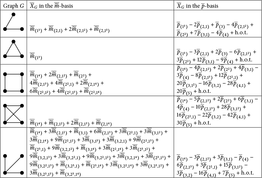


 Open access