


1 Introduction
1.1 Orbifold Donaldson–Thomas theory
Donaldson–Thomas (DT) theory, originally formulated in [Reference Thomas36], studies generating series of the degrees of virtual classes of Hilbert schemes of curves and points on a given Calabi–Yau
 $3$
-fold. Similarly, one can study the same generating series for a Calabi–Yau orbifold
$3$
-fold. Similarly, one can study the same generating series for a Calabi–Yau orbifold
 $\mathcal {X}$
of dimension three. Precise assumptions for the orbifolds we study here are given in Definition 2.1.
$\mathcal {X}$
of dimension three. Precise assumptions for the orbifolds we study here are given in Definition 2.1.
We focus here on the invariants for Hilbert schemes of points. For a given class
 $\alpha $
in the numerical Grothendieck-group
$\alpha $
in the numerical Grothendieck-group
 $\mathrm {N}_0(\mathcal {X})$
of
$\mathrm {N}_0(\mathcal {X})$
of
 $0$
-dimensional sheaves on
$0$
-dimensional sheaves on
 $\mathcal {X}$
, [Reference Olsson and Starr32] define a Hilbert scheme
$\mathcal {X}$
, [Reference Olsson and Starr32] define a Hilbert scheme
 $$ \begin{align*} \mathrm{Hilb}^\alpha(\mathcal{X}) \end{align*} $$
of substacks
 $\mathcal {Z}\subset \mathcal {X}$
of class
$\mathcal {Z}\subset \mathcal {X}$
of class
 $[\mathcal {O}_{\mathcal {Z}}]=\alpha $
. This Hilbert scheme can be equipped with a perfect obstruction theory by describing it as a moduli space of ideal sheaves. Using [Reference Behrend and Fantechi5], this defines a virtual cycle and a virtual structure sheaf
$[\mathcal {O}_{\mathcal {Z}}]=\alpha $
. This Hilbert scheme can be equipped with a perfect obstruction theory by describing it as a moduli space of ideal sheaves. Using [Reference Behrend and Fantechi5], this defines a virtual cycle and a virtual structure sheaf
 $\mathcal {O}^{\mathrm {vir}}_{\mathrm {Hilb}^\alpha (\mathcal {X})}\in K\left(\mathrm {Hilb}^\alpha (\mathcal {X})\right)$
. After twisting by a square root
$\mathcal {O}^{\mathrm {vir}}_{\mathrm {Hilb}^\alpha (\mathcal {X})}\in K\left(\mathrm {Hilb}^\alpha (\mathcal {X})\right)$
. After twisting by a square root
 $\mathcal {K}_{\mathrm {vir}}^{\frac {1}{2}}$
of the virtual canonical bundle, we obtain the twisted virtual structure sheaf
$\mathcal {K}_{\mathrm {vir}}^{\frac {1}{2}}$
of the virtual canonical bundle, we obtain the twisted virtual structure sheaf
This twist was introduced and motivated in [Reference Nekrasov and Okounkov27]. We study DT generating series
 $$ \begin{align} \mathsf{Z}(\mathcal{X}) := \sum_{\alpha \in \mathrm{N}_0(\mathcal{X})} q^{\alpha} \chi\left(\mathrm{Hilb}^\alpha(\mathcal{X}), \widehat{\mathcal{O}}^{\mathrm{vir}}\right). \end{align} $$
Here we take
 $\mathcal {X}$
to be either projective or toric. In the latter case, the Euler characteristic is defined via localization.
$\mathcal {X}$
to be either projective or toric. In the latter case, the Euler characteristic is defined via localization.
1.1.1 Main result
Our main theorem is a computation of the equivariant K-theoretic DT generating series
 $\mathsf {Z}\left([\mathbb {C}^3/\mu _r],q_0,\dots ,q_{r-1}\right)$
, where the variables
$\mathsf {Z}\left([\mathbb {C}^3/\mu _r],q_0,\dots ,q_{r-1}\right)$
, where the variables
 $q_i$
correspond to basis elements of
$q_i$
correspond to basis elements of
 $\mathrm {N}_0\left([\mathbb {C}^3/\mu _r]\right)=\mathbb {Z}^{\oplus r}$
, as explained in Example 2.5.
$\mathrm {N}_0\left([\mathbb {C}^3/\mu _r]\right)=\mathbb {Z}^{\oplus r}$
, as explained in Example 2.5.
Theorem 5.1. Let
 $\mathsf {T}=(\mathbb {C}^*)^3$
, acting on
$\mathsf {T}=(\mathbb {C}^*)^3$
, acting on
 $\mathbb {C}^3$
with weights
$\mathbb {C}^3$
with weights
 $(t_1,t_2,t_3)$
. The
$(t_1,t_2,t_3)$
. The
 $\mathsf {T}$
-equivariant K-theoretic degree
$\mathsf {T}$
-equivariant K-theoretic degree
 $0$
DT generating series for
$0$
DT generating series for
 $[\mathbb {C}^3/\mu _r]$
, with
$[\mathbb {C}^3/\mu _r]$
, with
 $\mu _r$
acting on
$\mu _r$
acting on
 $\mathbb {C}^3$
with weight
$\mathbb {C}^3$
with weight
 $(1,r-1,0)$
, is
$(1,r-1,0)$
, is
 $$ \begin{align*} \mathsf{Z}\left([\mathbb{C}^3/\mu_r],q_0,\dots,q_{r-1}\right) = \mathrm{PExp}\,\left(\mathsf{F}_r(q)+\mathsf{F}_r^{\mathrm{col}}(q_0,\dots,q_{r-1})\right), \end{align*} $$
where

where
 $\kappa =t_1t_2t_3$
,
$\kappa =t_1t_2t_3$
,
 $q=q_0\cdots q_{r-1}$
,
$q=q_0\cdots q_{r-1}$
,
 $q_{[i,j]}=q_i\cdots q_j$
,
$q_{[i,j]}=q_i\cdots q_j$
,
 $[w]=w^{1/2}-w^{-1/2}$
, and
$[w]=w^{1/2}-w^{-1/2}$
, and
 $\mathrm {PExp}\left(-\right)$
denotes the plethystic exponential, whose precise definition we give in Section 3.2.1.
$\mathrm {PExp}\left(-\right)$
denotes the plethystic exponential, whose precise definition we give in Section 3.2.1.
This formula was conjectured in [Reference Cirafici13, Conj. 2]. In [Reference Cao, Kool and Monavari11, Cor. 6.2] it was shown to follow from corresponding conjectural formula for 4-folds. We follow here the notation in [Reference Cao, Kool and Monavari11, Cor. 6.2]. Note that we don’t require a sign in front of our variable
 $q_0$
as our chosen twist for the twisted virtual structure sheaf includes the sign
$q_0$
as our chosen twist for the twisted virtual structure sheaf includes the sign
 $(-1)^{n_0}$
.
$(-1)^{n_0}$
.
1.1.2 Colored plane partitions
The generating series we study are (equivariant) K-theoretic refinements of more classical numerical Donaldson–Thomas invariants
 $$ \begin{align} \mathsf{Z}^{\mathrm{num}}(\mathcal{X}) := \sum_{\alpha \in \mathrm{N}_0(\mathcal{X})} q^{\alpha} \chi\left(\mathrm{Hilb}^\alpha(\mathcal{X}), \nu\right), \end{align} $$
defined using Euler characteristics weighted by the Behrend function
 $\nu $
. If
$\nu $
. If
 $\mathcal {X}=[\mathbb {C}^3/G]$
for some finite abelian subgroup
$\mathcal {X}=[\mathbb {C}^3/G]$
for some finite abelian subgroup
 $G\subset \mathrm {SL}(3)$
, these generating series turn out to be signed counts of colored plane partitions, as seen in [Reference Young39, Appendix A].
$G\subset \mathrm {SL}(3)$
, these generating series turn out to be signed counts of colored plane partitions, as seen in [Reference Young39, Appendix A].
Plane partitions are finite subsets
 $\pi $
of
$\pi $
of
 $\mathbb {Z}_{\geq 0}^3$
, such that if
$\mathbb {Z}_{\geq 0}^3$
, such that if
 $(i+1,j,k)$
,
$(i+1,j,k)$
,
 $(i,j+1,k)$
or
$(i,j+1,k)$
or
 $(i,j,k+1)$
are contained in
$(i,j,k+1)$
are contained in
 $\pi $
, then so is
$\pi $
, then so is
 $(i,j,k)$
. By labeling each box
$(i,j,k)$
. By labeling each box
 $(i,j,k)$
by the monomial
$(i,j,k)$
by the monomial
 $x^iy^jz^k$
, these correspond to
$x^iy^jz^k$
, these correspond to
 $\mathsf {T}$
-fixed
$\mathsf {T}$
-fixed
 $0$
-dimensional subschemes of
$0$
-dimensional subschemes of
 $\mathbb {C}^3$
, which must be cut out by monomial ideals in
$\mathbb {C}^3$
, which must be cut out by monomial ideals in
 $\mathbb {C}[x,y,z]$
. The action of G on
$\mathbb {C}[x,y,z]$
. The action of G on
 $\mathbb {C}^3$
corresponds to an action on
$\mathbb {C}^3$
corresponds to an action on
 $\mathbb {C}[x,y,z]$
whose weight spaces are spanned by
$\mathbb {C}[x,y,z]$
whose weight spaces are spanned by
 $\mathbb {C} x^iy^jz^k$
. The boxes
$\mathbb {C} x^iy^jz^k$
. The boxes
 $(i,j,k)$
of the plane partition are then colored by the characters of G of the corresponding
$(i,j,k)$
of the plane partition are then colored by the characters of G of the corresponding
 $\mathbb {C} x^iy^jz^k$
.
$\mathbb {C} x^iy^jz^k$
.
For
 $G=\mu _r$
acting with weights
$G=\mu _r$
acting with weights
 $(1,-1,0)$
[Reference Young39] computes the generating series to be
$(1,-1,0)$
[Reference Young39] computes the generating series to be
 $$ \begin{align} \mathsf{Z}^{\mathrm{num}}\left([\mathbb{C}^3/\mu_r],-q_0,q_1,\dots,q_{r-1}\right) = \mathrm{PExp}\,\left(\frac{-1}{[q][q^{-1}]}\left(r+\sum_{0<i\leq j<r}\left(q_{[i,j]}+q_{[i,j]}^{-1}\right)\right)\right). \end{align} $$
As explained in [Reference Young39, Appendix A], the sign in front of the formal variable
 $q_0$
comes from relating the combinatorial count of colored plane partitions to the Behrend-function weighted count. Our main computation, Theorem 5.1, refines that result to equivariant K-theoretic DT invariants.
$q_0$
comes from relating the combinatorial count of colored plane partitions to the Behrend-function weighted count. Our main computation, Theorem 5.1, refines that result to equivariant K-theoretic DT invariants.
1.1.3 Orbifold crepant resolution conjecture
An important conjecture in orbifold DT theory is the crepant resolution conjecture [Reference Bryan, Cadman and Young9]. Given a
 $3$
-dimensional Calabi–Yau orbifold
$3$
-dimensional Calabi–Yau orbifold
 $\mathcal {X}$
, take a crepant resolution
$\mathcal {X}$
, take a crepant resolution

This exists using [Reference Bridgeland, King and Reid8], who also give an equivalence between the derived categories of coherent sheaves on
 $\mathcal {X}$
and Y. This lets us identify the numerical Grothendieck groups
$\mathcal {X}$
and Y. This lets us identify the numerical Grothendieck groups
 $\mathrm {N}_c(\mathcal {X})$
and
$\mathrm {N}_c(\mathcal {X})$
and
 $\mathrm {N}_c(Y)$
. However, this identification does not respect the filtration by dimension of supports. For
$\mathrm {N}_c(Y)$
. However, this identification does not respect the filtration by dimension of supports. For
 $\mathcal {X}$
satisfying the Hard Lefschetz condition, the crepant resolution conjecture identifies a version of the DT generating series of
$\mathcal {X}$
satisfying the Hard Lefschetz condition, the crepant resolution conjecture identifies a version of the DT generating series of
 $\mathcal {X}$
with the one of Y. We state here the conjecture for the DT invariants of Hilbert schemes of points on
$\mathcal {X}$
with the one of Y. We state here the conjecture for the DT invariants of Hilbert schemes of points on
 $\mathcal {X}$
.
$\mathcal {X}$
.
Conjecture [Reference Bryan, Cadman and Young9, Conj. 2],[Reference Cao, Kool and Monavari11, Cor. 6.3]
In the above setup, there is an identity
 $$ \begin{align*} \mathsf{Z}^{\mathrm{DT}}_0(\mathcal{X}) = \mathsf{Z}^{\mathrm{DT}}_0(Y)\mathsf{Z}^{\mathrm{PT}}_{\mathrm{exc}}(Y)\widetilde{\mathsf{Z}}^{\mathrm{PT}}_{\mathrm{exc}}(Y). \end{align*} $$
Here
 $\mathsf {Z}^{\mathrm {PT}}_{\mathrm {exc}}(Y)$
is the PT generating series of curves in Y which are contracted to points in the singular locus of X, and
$\mathsf {Z}^{\mathrm {PT}}_{\mathrm {exc}}(Y)$
is the PT generating series of curves in Y which are contracted to points in the singular locus of X, and
 $\widetilde {\mathsf {Z}}^{\mathrm {PT}}_{\mathrm {exc}}(Y)$
is related to it by a change of variables.
$\widetilde {\mathsf {Z}}^{\mathrm {PT}}_{\mathrm {exc}}(Y)$
is related to it by a change of variables.
For numerical DT-invariants the above crepant resolution conjecture has been shown using wall-crossing in [Reference Calabrese10]. The curve-counting version was shown in the case of toric orbifolds with transverse A-singularities in [Reference Ross35], and for general orbifolds using wall-crossing in [Reference Viktor Beentjes, Calabrese and Vold Rennemo4]. The natural equivariant K-theoretically refined versions of this conjecture have been proposed for specific crepant resolutions in [Reference Cao, Kool and Monavari11, Cor. 6.3].
Our main computation gives the equivariant K-theoretic count for the left-hand side in the case
 $\mathcal {X}=[\mathbb {C}^3/\mu _r]$
. Moreover, we introduce a general setup of factorization techniques to study DT invariants of Hilbert schemes of points on orbifolds, which allows us to show in Proposition 4.6 that
$\mathcal {X}=[\mathbb {C}^3/\mu _r]$
. Moreover, we introduce a general setup of factorization techniques to study DT invariants of Hilbert schemes of points on orbifolds, which allows us to show in Proposition 4.6 that
 $\mathsf {Z}^{\mathrm {DT}}_0(Y)$
divides
$\mathsf {Z}^{\mathrm {DT}}_0(Y)$
divides
 $\mathsf {Z}^{\mathrm {DT}}_0(\mathcal {X})$
in a controlled way for any
$\mathsf {Z}^{\mathrm {DT}}_0(\mathcal {X})$
in a controlled way for any
 $\mathcal {X}$
satisfying a technical condition.
$\mathcal {X}$
satisfying a technical condition.
1.2 Strategy
We use two main tools in computing the generating series of our main result: A version for orbifolds of the factorization techniques used in [Reference Okounkov31] to prove Nekrasov’s formula, and a semi-equivariant extension of the argument used in [Reference Young39], which allows us to compute a limit of the generating series in the equivariant parameters. By the rigidity principle, introduced in [Reference Okounkov31], this determines our generating series.
1.2.1 Factorization for orbifolds
In [Reference Okounkov31] and [Reference Kool and Rennemo22], factorization for schemes is used in the following way. Take (twisted) virtual structure sheaves, defined using quiver-theoretic descriptions of Hilbert schemes of points on
 $X=\mathbb {C}^3$
. It is shown that their pushforwards to
$X=\mathbb {C}^3$
. It is shown that their pushforwards to
 $\mathrm {Sym}^n(X)$
along the Hilbert-Chow morphism satisfy a factorization property. That roughly means the following. Take the open locus
$\mathrm {Sym}^n(X)$
along the Hilbert-Chow morphism satisfy a factorization property. That roughly means the following. Take the open locus
where the two collections of points are disjoint from each other. Then on U we have
 $$ \begin{align*} \mathrm{HC}_{n_1 *}\widehat{\mathcal{O}}_{n_1}^{\mathrm{vir}}\boxtimes\mathrm{HC}_{n_2 *}\widehat{\mathcal{O}}_{n_2}^{\mathrm{vir}}\cong \mathrm{HC}_{n_1+n_2 *}\widehat{\mathcal{O}}_{n_1+n_2}^{\mathrm{vir}} \end{align*} $$
with certain compatibilities under consecutive splittings. Here
 $\mathrm {HC}_n: \mathrm {Hilb}^n(X)\to \mathrm {Sym}^n(X)$
denotes the Hilbert-Chow morphism. Under this condition, it can be shown that the generating series of Euler characteristics of the virtual structure sheaves is the plethystic exponential of a generating series of Euler characteristics of certain classes
$\mathrm {HC}_n: \mathrm {Hilb}^n(X)\to \mathrm {Sym}^n(X)$
denotes the Hilbert-Chow morphism. Under this condition, it can be shown that the generating series of Euler characteristics of the virtual structure sheaves is the plethystic exponential of a generating series of Euler characteristics of certain classes
 $\mathcal {G}_n$
on X
$\mathcal {G}_n$
on X
 $$ \begin{align*} \mathsf{Z}(X) = 1+\sum_{n>0} q^{n} \chi\left(\mathrm{Hilb}^{n}(X),\widehat{\mathcal{O}}^{\mathrm{vir}}_{\mathrm{Hilb}^{n}(X)}\right) = \mathrm{PExp}\,\left(\sum_{n>0}q^{n} \chi(X,\mathcal{G}_{n})\right). \end{align*} $$
In Section 3 we develop a generalization of the notion of factorizable systems, which applies in the orbifold setting. One of the difficulties is to figure out a suitable replacement for the number of points and the symmetric product. For orbifolds, we use
 $0$
-dimensional effective numerical K-theory classes
$0$
-dimensional effective numerical K-theory classes
 $\alpha \in \mathrm {N}_0(\mathcal {X})$
instead of
$\alpha \in \mathrm {N}_0(\mathcal {X})$
instead of
 $n\in \mathbb {N}$
. Fixing a coarse moduli space of the orbifold
$n\in \mathbb {N}$
. Fixing a coarse moduli space of the orbifold
 $\pi :\mathcal {X}\to X$
, we use the symmetric product
$\pi :\mathcal {X}\to X$
, we use the symmetric product
 $\mathrm {Sym}^{\pi _*(\alpha )}(X)$
, where
$\mathrm {Sym}^{\pi _*(\alpha )}(X)$
, where
 $\pi _*(\alpha )$
can be identified with an integer. We find a factorization property for virtual structure sheaves pushed forward along the morphisms
$\pi _*(\alpha )$
can be identified with an integer. We find a factorization property for virtual structure sheaves pushed forward along the morphisms
 $$ \begin{align*} \mathrm{Hilb}^{\alpha}(\mathcal{X}) \to \mathrm{Sym}^{\pi_*(\alpha)}(X). \end{align*} $$
Importantly, the factorization property is only satisfied with respect to splittings of the
 $0$
-dimensional K-theory class
$0$
-dimensional K-theory class
 $\alpha $
and not its image
$\alpha $
and not its image
 $\pi _*(\alpha )$
in X.
$\pi _*(\alpha )$
in X.
A K-theory class of a substack of an orbifold can potentially be written as a sum of effective K-theory classes, which are not K-theory classes of substacks. This is also apparent when thinking of colored (plane) partitions, where we may have the following situation. The set of boxes of a colored (plane) partition may potentially be partitioned into two subsets in such a way that the count of colored boxes in (at least) one of the subsets can not itself be obtained from a colored (plane) partition; see, for example Figure 1. So we have to additionally restrict to classes in a factorization index set
 $$ \begin{align*} I := \left\{\alpha\ |\ \mathrm{Hilb}^{\alpha}(\mathcal{X})\neq \emptyset\right\}, \end{align*} $$
so that we only allow splittings of K-theory classes into K-theory classes which also come from the Hilbert scheme of points. Details of this step, which is not necessary in the scheme case, are discussed in Section 3.1.1.
A version of our main theorem about such factorizable system is the following, which allows us to compute generating series of their Euler characteristics in a simple way.
Theorem (Corollary 3.25)
Let I be a factorization index semigroup. For a factorizable system
 $\mathcal {F}_{\alpha }$
on
$\mathcal {F}_{\alpha }$
on
 $\mathrm {Sym}^{b(\alpha )}(X)$
, there exist classes
$\mathrm {Sym}^{b(\alpha )}(X)$
, there exist classes
 $[\mathcal {G}_{\alpha }]$
on X such that
$[\mathcal {G}_{\alpha }]$
on X such that
 $$ \begin{align*} 1 + \sum_{\alpha\in I} q^{\alpha} \chi\left(\mathrm{Sym}^{b(\alpha)}(X),\mathcal{F}_{\alpha}\right) = \mathrm{PExp}\,\left(\sum_{\alpha\in I}q^{\alpha} \chi(X,\mathcal{G}_{\alpha})\right), \end{align*} $$
where
 $b(\alpha )\in \mathbb {Z}$
is defined as the integer corresponding to
$b(\alpha )\in \mathbb {Z}$
is defined as the integer corresponding to
 $\pi _*(\alpha )$
under the isomorphism
$\pi _*(\alpha )$
under the isomorphism
 $\mathrm {N}_0(X)\cong \mathbb {Z}$
.
$\mathrm {N}_0(X)\cong \mathbb {Z}$
.
The construction of the classes
 $\mathcal {G}_\alpha $
involves tracking possible sequences of splittings of
$\mathcal {G}_\alpha $
involves tracking possible sequences of splittings of
 $\alpha $
into various parts. The resulting classes
$\alpha $
into various parts. The resulting classes
 $\mathcal {G}_\alpha $
in the plethystic exponential are classes on X, the coarse space of the orbifold
$\mathcal {G}_\alpha $
in the plethystic exponential are classes on X, the coarse space of the orbifold
 $\mathcal {X}$
. One additional feature in the orbifold case is that the construction of these classes allows us to restrict the support of many of these classes to the complement of the nonstacky locus in X. As this is often much smaller, the possible poles of these functions computed by localization can be restricted.
$\mathcal {X}$
. One additional feature in the orbifold case is that the construction of these classes allows us to restrict the support of many of these classes to the complement of the nonstacky locus in X. As this is often much smaller, the possible poles of these functions computed by localization can be restricted.
In Section 4 we prove that (twisted) virtual structure sheaves are factorizable and obtain a strong result about the generating series of Euler characteristics
 $$ \begin{align*} \mathsf{Z}(\mathcal{X}) = 1+\sum_{\alpha\in I} q^{\alpha} \chi\left(\mathrm{Hilb}^{\alpha}(\mathcal{X}),\widehat{\mathcal{O}}^{\mathrm{vir}}_{\mathrm{Hilb}^{\alpha}(\mathcal{X})}\right) = \mathrm{PExp}\,\left(\sum_{\alpha\in I}q^{\alpha} \chi(X,\mathcal{G}_{\alpha})\right) \end{align*} $$
in Corollary 3.25. Note here a technical requirement that I is closed under addition, which is satisfied in the examples we consider.
Finally, we develop a technique of compatible factorizations, which allows us to compare the classes
 $\mathcal {G}_\alpha $
constructed using different factorizable sequences, which are compatible along an embedding in a suitable sense. This yields relations between the generating series for
$\mathcal {G}_\alpha $
constructed using different factorizable sequences, which are compatible along an embedding in a suitable sense. This yields relations between the generating series for
 $\mathcal {X}$
and its crepant resolution in Proposition 4.6.
$\mathcal {X}$
and its crepant resolution in Proposition 4.6.
Remark. We further explain in Section 3.1.5 how the techniques involved in extending factorization to work in the orbifold setting also apply in a more general “relative” setting with a morphism
 $$ \begin{align*} f:\mathcal{Y} \to X, \end{align*} $$
from an orbifold to a connected scheme. This could potentially be useful for studying crepant resolutions or fibered geometries.
1.2.2 Limit-equivariant slicing
As in [Reference Okounkov31], we use the rigidity principle to show that, except for certain fixed factors, which we compute, the functions in the plethystic exponential depend only on
 $\kappa =t_1t_2t_3$
and not on the individual
$\kappa =t_1t_2t_3$
and not on the individual
 $t_i$
. This means it suffices to compute any limit
$t_i$
. This means it suffices to compute any limit
in the parameters
 $t_i$
that keeps
$t_i$
that keeps
 $\kappa $
fixed. [Reference Okounkov31] suggests a particular limit of this kind
$\kappa $
fixed. [Reference Okounkov31] suggests a particular limit of this kind
 $$ \begin{align} t_1,t_3\to 0,\ \lvert t_1 \rvert\ll\lvert t_3\rvert,\ \kappa\ \mathrm{fixed}, \end{align} $$
which admits a very simple formula in Proposition 5.4 for the limit contributions of each plane partition, computed using [Reference Nekrasov and Okounkov27, Appendix A].
In [Reference Young39], Young uses a slicing argument, where he decomposes a colored plane partition into monochrome slices, which are partitions. Then, working in a vector space ![]() , which has an orthonormal basis given by all partitions
, which has an orthonormal basis given by all partitions ![]() , he uses operators
, he uses operators
 $$ \begin{align*} \Gamma_\pm(x) = \mathrm{exp}\left(\sum_l \frac{x^l}{l}\alpha_{\pm l}\right) \end{align*} $$
which sum over all possible next or previous slices within a plane partition. To compute the desired count of colored plane partitions he introduces weight operators
which multiply by the formal variables
 $q_i$
. Computing commutators of these operators allows the full computation of the generating series
$q_i$
. Computing commutators of these operators allows the full computation of the generating series
where ![]() is the empty partition and
is the empty partition and ![]() .
.
A fully equivariant version of this slicing argument is not known, because it is not clear that the equivariant weight of each colored plane partition in the generating series can be computed from certain weights of each slice. However, using the particular limit (4), we can compute the limit contributions of each colored plane partition from simple weights on each slice in Proposition 5.4. So, we introduce a limit weight operator
into Young’s slicing argument, which allow us to use the argument to compute the desired limit
 $\overrightarrow {\mathsf {Z}}\left([\mathbb {C}^3/\mu _r],\mathbf {q}\right)$
of the generating series in Section 5.2 to complete the proof of our main theorem.
$\overrightarrow {\mathsf {Z}}\left([\mathbb {C}^3/\mu _r],\mathbf {q}\right)$
of the generating series in Section 5.2 to complete the proof of our main theorem.
1.3 Future directions
1.3.1 Extension to
 $\mu _2\times \mu _2$

A formula similar to (3) was proven in the unrefined case for
 $[\mathbb {C}^3/\mu _2\times \mu _2]$
in [Reference Young39], where
$[\mathbb {C}^3/\mu _2\times \mu _2]$
in [Reference Young39], where
 $G=\mu _2\times \mu _2$
acts as the group of diagonal matrices with determinant
$G=\mu _2\times \mu _2$
acts as the group of diagonal matrices with determinant
 $1$
that square to the identity. Refined formulas were computed in [Reference Cao, Kool and Monavari11, Cor. 6.2], again assuming a corresponding conjectural formula for 4-folds. It would be interesting to adapt the techniques of this paper to also compute that case.
$1$
that square to the identity. Refined formulas were computed in [Reference Cao, Kool and Monavari11, Cor. 6.2], again assuming a corresponding conjectural formula for 4-folds. It would be interesting to adapt the techniques of this paper to also compute that case.
1.3.2 Calabi–Yau 4-folds
Donaldson–Thomas invariants for Calabi–Yau 4-folds have recently been introduced by [Reference Borisov and Joyce6] and [Reference Oh and Thomas29]. Factorization techniques have been used by [Reference Kool and Rennemo22] to compute the equivariant K-theoretic DT invariants of Hilbert schemes of points on
 $\mathbb {C}^4$
confirming a conjecture by Nekrasov and Piazzalunga. They use a combination of factorization techniques and localization, and finally relate a specialization of their generating series to the DT generating series of Hilbert schemes of points on
$\mathbb {C}^4$
confirming a conjecture by Nekrasov and Piazzalunga. They use a combination of factorization techniques and localization, and finally relate a specialization of their generating series to the DT generating series of Hilbert schemes of points on
 $\mathbb {C}^3$
, which is given by Nekrasov’s formula, proven in [Reference Okounkov31].
$\mathbb {C}^3$
, which is given by Nekrasov’s formula, proven in [Reference Okounkov31].
We are working on extending the computation here to the case of
 $[\mathbb {C}^4/\mu _r]$
, with
$[\mathbb {C}^4/\mu _r]$
, with
 $\mu _r$
acting on the first two coordinates. In fact, following the argument in [Reference Kool and Rennemo22], our main theorem must be used in place of Nekrasov’s formula for an orbifold computation.
$\mu _r$
acting on the first two coordinates. In fact, following the argument in [Reference Kool and Rennemo22], our main theorem must be used in place of Nekrasov’s formula for an orbifold computation.
2 Setup
2.1 Orbifolds
Definition 2.1. We fix some conventions. Throughout, we write orbifold for a smooth separated finite type DM-stack with generically trivial stabilizers over
 $\mathbb {C}$
. We work with various types of orbifolds. We consider an orbifold
$\mathbb {C}$
. We work with various types of orbifolds. We consider an orbifold
 $\mathcal {X}$
to be
$\mathcal {X}$
to be
-
• (quasi-)projective if it is (quasi-)projective in the sense of [Reference Kresch, Abramovich, Bertram, Katzarkov, Pandharipande and Thaddeus23, Def. 5.5]. In particular, it has a (quasi-)projective coarse moduli space
$\pi :\mathcal {X}\to X$
, -
• equipped with a
$\mathsf {T}$
-action if it comes equipped with an action by a connected reductive algebraic group
$\mathsf {T}$
, which will often be a torus, -
• Calabi–Yau if
$\mathcal {K}_{\mathcal {X}}\cong \mathcal {O}_{\mathcal {X}}$
. In the
$\mathsf {T}$
-equivariant case, we write
$\kappa $
for the
$\mathsf {T}$
-weight of
$\mathcal {K}_{\mathcal {X}}$
, such that
$\mathcal {K}_{\mathcal {X}}\cong \kappa \mathcal {O}_{\mathcal {X}}$
as
$\mathsf {T}$
-equivariant sheaves. -
• toric if
$\mathcal {X}$
is a smooth separated toric DM-stack in the sense of [Reference Borisov, Chen and Smith7, Reference Fantechi, Mann and Nironi16]. In this case, there is a
$\mathsf {T}=(\mathbb {C}^*)^{\dim (\mathcal {X})}$
-action on
$\mathcal {X}$
.


In the
 $\mathsf {T}$
-equivariant and the toric cases, we will always assume that the stack of fixed points
$\mathsf {T}$
-equivariant and the toric cases, we will always assume that the stack of fixed points
 $\mathcal {X}^{\mathsf {T}}$
is nonempty. If
$\mathcal {X}^{\mathsf {T}}$
is nonempty. If
 $\mathcal {X}$
is Calabi–Yau, that makes
$\mathcal {X}$
is Calabi–Yau, that makes
 $\kappa $
uniquely defined.
$\kappa $
uniquely defined.
In the toric case, we have the following well-known local description, which allows us to understand the
 $\mathsf {T}$
-fixed points in the Hilbert scheme of points and simplify computations.
$\mathsf {T}$
-fixed points in the Hilbert scheme of points and simplify computations.
Lemma 2.2. A d-dimensional toric orbifold
 $\mathcal {X}$
with
$\mathcal {X}$
with
 $\mathcal {X}^{\mathsf {T}}\neq \emptyset $
is étale locally isomorphic to
$\mathcal {X}^{\mathsf {T}}\neq \emptyset $
is étale locally isomorphic to
 $[\mathbb {C}^d/G]$
for some finite abelian diagonally embedded subgroup
$[\mathbb {C}^d/G]$
for some finite abelian diagonally embedded subgroup
 $G\subset \mathrm {GL}(d)$
. If
$G\subset \mathrm {GL}(d)$
. If
 $\mathcal {X}$
is Calabi–Yau, then
$\mathcal {X}$
is Calabi–Yau, then
 $G\subset \mathrm {SL}(d)$
.
$G\subset \mathrm {SL}(d)$
.
Proof. Let
 $\mathcal {X}$
be a d-dimensional toric orbifold with associated stacky fan
$\mathcal {X}$
be a d-dimensional toric orbifold with associated stacky fan
 $\Sigma $
. Then
$\Sigma $
. Then
 $$ \begin{align*} \mathcal{X}^{\mathsf{T}}\neq \emptyset\ \Leftrightarrow\ \Sigma\text{ has a }d\text{-dimensional cone}. \end{align*} $$
The
 $\Leftarrow $
direction follows immediately from [Reference Borisov, Chen and Smith7, Prop. 4.3]. For the
$\Leftarrow $
direction follows immediately from [Reference Borisov, Chen and Smith7, Prop. 4.3]. For the
 $\Rightarrow $
direction, if
$\Rightarrow $
direction, if
 $\Sigma $
has no d-dimensional cone, then
$\Sigma $
has no d-dimensional cone, then
 $\mathcal {X}\cong \mathcal {X}'\times (\mathbb {C}^*)^k$
for some
$\mathcal {X}\cong \mathcal {X}'\times (\mathbb {C}^*)^k$
for some
 $k>0$
with
$k>0$
with
 $\mathsf {T}$
acting by
$\mathsf {T}$
acting by
 $(t_{d-k+1},\dots ,t_{d})$
on
$(t_{d-k+1},\dots ,t_{d})$
on
 $(\mathbb {C}^*)^k$
, so
$(\mathbb {C}^*)^k$
, so
 $\mathcal {X}^{\mathsf {T}}=\emptyset $
.
$\mathcal {X}^{\mathsf {T}}=\emptyset $
.
Now the first part of the lemma follows from [Reference Borisov, Chen and Smith7, Prop. 4.3]. If
 $\mathcal {X}$
is Calabi–Yau, then the fiber of the canonical bundle over the fixed point in
$\mathcal {X}$
is Calabi–Yau, then the fiber of the canonical bundle over the fixed point in
 $[\mathbb {C}^d/G]$
has the structure of a G-representation. Viewing G as a subgroup of
$[\mathbb {C}^d/G]$
has the structure of a G-representation. Viewing G as a subgroup of
 $\mathrm {GL}(d)$
, this is the determinant, and triviality of the canonical bundle hence implies
$\mathrm {GL}(d)$
, this is the determinant, and triviality of the canonical bundle hence implies
 $G\subset \mathrm {SL}(d)$
.
$G\subset \mathrm {SL}(d)$
.
Definition 2.3. Because we require an orbifold
 $\mathcal {X}$
to have generically trivial stabilizers, there exists an open dense subscheme U in
$\mathcal {X}$
to have generically trivial stabilizers, there exists an open dense subscheme U in
 $\mathcal {X}$
. We call this the nonstacky locus. The coarse moduli space
$\mathcal {X}$
. We call this the nonstacky locus. The coarse moduli space
 $\pi :\mathcal {X}\to X$
restricts to the identity on U, making U an open subscheme of X. We denote by S its complement with the reduced subscheme structure.
$\pi :\mathcal {X}\to X$
restricts to the identity on U, making U an open subscheme of X. We denote by S its complement with the reduced subscheme structure.
Remark 2.4. While technically there are different choices of U, since one could remove a lower-dimensional closed subset from U, there is always a canonical maximal choice of U, which we consider as given throughout. For example, for any global quotient orbifold
 $[V/G]$
, we take U to be
$[V/G]$
, we take U to be
 $[\tilde {U}/G]$
, where
$[\tilde {U}/G]$
, where
 $\tilde {U}$
is the open subscheme where G acts freely.
$\tilde {U}$
is the open subscheme where G acts freely.
2.2 Moduli spaces on orbifolds
Studying generating series of orbifold DT invariants, we encounter various types of moduli spaces on orbifolds. Let
 $\mathcal {X}$
be an orbifold, possibly equipped with a
$\mathcal {X}$
be an orbifold, possibly equipped with a
 $\mathsf {T}$
-action.
$\mathsf {T}$
-action.
2.2.1 Hilbert schemes of points on orbifolds
Similar to [Reference Bayer, Craw and Zhang3, Section 5.1], we consider the Grothendieck group
 $K_c(\mathcal {X})$
of
$K_c(\mathcal {X})$
of
 $D^b_c(\mathcal {X})$
, the compactly supported objects in the bounded derived category
$D^b_c(\mathcal {X})$
, the compactly supported objects in the bounded derived category
 $D^b(\mathcal {X})$
of coherent sheaves on
$D^b(\mathcal {X})$
of coherent sheaves on
 $\mathcal {X}$
. The numerical Grothendieck group
$\mathcal {X}$
. The numerical Grothendieck group
 $\mathrm {N}_c(\mathcal {X})$
is
$\mathrm {N}_c(\mathcal {X})$
is
 $K_c(\mathcal {X})$
modulo the kernel of the Euler pairing
$K_c(\mathcal {X})$
modulo the kernel of the Euler pairing
 $$ \begin{align*} \chi(-,-) : K(\mathrm{D}^b_{\mathrm{perf}}(\mathcal{X}))\times K_c(\mathcal{X}) \to \mathbb{Z} \end{align*} $$
on
 $K_c(\mathcal {X})$
. We will focus on
$K_c(\mathcal {X})$
. We will focus on
 $\mathrm {N}_0(\mathcal {X})$
, the subgroup generated by 0-dimensional sheaves. For a given class
$\mathrm {N}_0(\mathcal {X})$
, the subgroup generated by 0-dimensional sheaves. For a given class
 $\alpha \in \mathrm {N}_0(\mathcal {X})$
, [Reference Olsson and Starr32] define a Hilbert scheme
$\alpha \in \mathrm {N}_0(\mathcal {X})$
, [Reference Olsson and Starr32] define a Hilbert scheme
 $$ \begin{align*} \mathrm{Hilb}^\alpha(\mathcal{X}) \end{align*} $$
of substacks
 $\mathcal {Z}\subset \mathcal {X}$
of class
$\mathcal {Z}\subset \mathcal {X}$
of class
 $[\mathcal {O}_{\mathcal {Z}}]=\alpha $
. Even though
$[\mathcal {O}_{\mathcal {Z}}]=\alpha $
. Even though
 $\mathcal {X}$
is an orbifold, this turns out to be an algebraic space, as the substacks
$\mathcal {X}$
is an orbifold, this turns out to be an algebraic space, as the substacks
 $\mathcal {Z}$
, which it parametrizes, do not have automorphisms. Although these Hilbert spaces are algebraic spaces and such substacks are more than just collections of points, we will refer to these
$\mathcal {Z}$
, which it parametrizes, do not have automorphisms. Although these Hilbert spaces are algebraic spaces and such substacks are more than just collections of points, we will refer to these
 $\mathrm {Hilb}^\alpha (\mathcal {X})$
as Hilbert schemes of points on
$\mathrm {Hilb}^\alpha (\mathcal {X})$
as Hilbert schemes of points on
 $\mathcal {X}$
, writing
$\mathcal {X}$
, writing ![]() .
.
Consider the subset of effective classes
Note that by definition,
 $\mathrm {Hilb}^0(\mathcal {X})$
is a point, and for
$\mathrm {Hilb}^0(\mathcal {X})$
is a point, and for
 $\alpha \neq 0$
the Hilbert scheme
$\alpha \neq 0$
the Hilbert scheme
 $\mathrm {Hilb}^\alpha (\mathcal {X})$
is only nonempty if
$\mathrm {Hilb}^\alpha (\mathcal {X})$
is only nonempty if
 $\alpha $
is effective.
$\alpha $
is effective.
Example 2.5. Given a finite abelian group G of order r acting on
 $\mathbb {C}^d$
as a diagonally embedded subgroup
$\mathbb {C}^d$
as a diagonally embedded subgroup
 $G\subset \mathrm {SL}(d)$
, we consider the global quotient stack
$G\subset \mathrm {SL}(d)$
, we consider the global quotient stack
 $\mathcal {X}=[\mathbb {C}^d/G]$
. Its numerical Grothendieck group of 0-dimensional sheaves is
$\mathcal {X}=[\mathbb {C}^d/G]$
. Its numerical Grothendieck group of 0-dimensional sheaves is
 $\mathrm {N}_0(\mathcal {X})=\mathbb {Z}^{\oplus r}$
. We see this as follows.
$\mathrm {N}_0(\mathcal {X})=\mathbb {Z}^{\oplus r}$
. We see this as follows.
Take the G-equivariant embedding of the origin into
 $\mathbb {C}^d$
and view it as a closed embedding
$\mathbb {C}^d$
and view it as a closed embedding
 $$ \begin{align*} p:\mathrm{B}{G}\hookrightarrow \mathcal{X}. \end{align*} $$
As
 $K(\mathrm {B}{G})\cong \mathbb {Z}^{\oplus r}$
spanned by the irreducible representations
$K(\mathrm {B}{G})\cong \mathbb {Z}^{\oplus r}$
spanned by the irreducible representations
 $\rho _0,\dots ,\rho _{r-1}$
of G, it suffices to show that
$\rho _0,\dots ,\rho _{r-1}$
of G, it suffices to show that
 $p_*$
is an isomorphism. Here and throughout, we assume that the
$p_*$
is an isomorphism. Here and throughout, we assume that the
 $\rho _i$
are labelled such that
$\rho _i$
are labelled such that
 $\rho _0$
is the trivial character.
$\rho _0$
is the trivial character.
To show that
 $p_*$
is surjective, take the class
$p_*$
is surjective, take the class
 $[\mathcal {F}]$
of a
$[\mathcal {F}]$
of a
 $0$
-dimensional coherent sheaf. Any sheaf can be deformed algebraically to be supported at the fixed point, so we may assume
$0$
-dimensional coherent sheaf. Any sheaf can be deformed algebraically to be supported at the fixed point, so we may assume
 $\mathcal {F}$
is supported at the origin. We show it is in the image of
$\mathcal {F}$
is supported at the origin. We show it is in the image of
 $p_*$
by induction on the length of
$p_*$
by induction on the length of
 $\mathcal {F}$
. This is trivial for length
$\mathcal {F}$
. This is trivial for length
 $0$
. Consider the short exact sequence
$0$
. Consider the short exact sequence
 $$ \begin{align*} 0\to \mathcal{F}' \to \mathcal{F} \to p_*p^*\mathcal{F} \to 0, \end{align*} $$
where
 $\mathcal {F}'$
is the kernel of the adjunction. By induction
$\mathcal {F}'$
is the kernel of the adjunction. By induction
 $[\mathcal {F}']$
is in the image of
$[\mathcal {F}']$
is in the image of
 $p_*$
as a sheaf of lower length than
$p_*$
as a sheaf of lower length than
 $\mathcal {F}$
. Hence,
$\mathcal {F}$
. Hence,
 $[\mathcal {F}]=[\mathcal {F}']+[p_*p^*\mathcal {F}]$
is also in the image of
$[\mathcal {F}]=[\mathcal {F}']+[p_*p^*\mathcal {F}]$
is also in the image of
 $p_*$
.
$p_*$
.
To show that
 $p_*$
is injective, it suffices to show that
$p_*$
is injective, it suffices to show that
 $p_*(\rho _i)\neq 0$
for all i. We take
$p_*(\rho _i)\neq 0$
for all i. We take
 $q:\mathcal {X}\to \mathrm {B}{G}$
given by the G-equivariant morphism to the point. This yields the nonvanishing classes
$q:\mathcal {X}\to \mathrm {B}{G}$
given by the G-equivariant morphism to the point. This yields the nonvanishing classes
 $q^*\rho _j$
. Using
$q^*\rho _j$
. Using
 $p\circ q=\mathrm {id}$
and the projection formula, we get
$p\circ q=\mathrm {id}$
and the projection formula, we get
 $$ \begin{align*} \chi\left(q^*\rho_j,p_*\rho_i\right)=\delta_{ij}, \end{align*} $$
which shows that the class
 $p_*(\rho _i)$
doesn’t vanish for any i.
$p_*(\rho _i)$
doesn’t vanish for any i.
2.2.2 Moduli of 0-dimensional sheaves on orbifolds
We additionally consider moduli of 0-dimensional sheaves on orbifolds. For schemes, [Reference Huybrechts and Lehn21, Ex. 4.3.6] shows that the moduli spaces of 0-dimensional sheaves are exactly the symmetric products of the base scheme. Following this, we use moduli of 0-dimensional sheaves on orbifolds as our analogues of symmetric products. The existence of such a moduli space can be collected as follows from the literature.
Proposition 2.6. Let
 $\mathcal {X}$
be an orbifold. Then there exists an algebraic stack
$\mathcal {X}$
be an orbifold. Then there exists an algebraic stack
 $\mathfrak {M}_0$
of zero-dimensional sheaves on
$\mathfrak {M}_0$
of zero-dimensional sheaves on
 $\mathcal {X}$
, which is locally of finite presentation and has affine diagonal. If
$\mathcal {X}$
, which is locally of finite presentation and has affine diagonal. If
 $\mathcal {X}$
is equipped with a
$\mathcal {X}$
is equipped with a
 $\mathsf {T}$
-action, so is
$\mathsf {T}$
-action, so is
 $\mathfrak {M}_0$
. Moreover, this stack has a good moduli space
$\mathfrak {M}_0$
. Moreover, this stack has a good moduli space
 $$ \begin{align*} \mathfrak{M}_0 \to M_0, \end{align*} $$
which also comes equipped with a
 $\mathsf {T}$
-action, compatible with the good moduli space maps.
$\mathsf {T}$
-action, compatible with the good moduli space maps.
Proof. Note that the
 $\mathsf {T}$
-action on good moduli space is induced by universality of a good moduli space if one exists.
$\mathsf {T}$
-action on good moduli space is induced by universality of a good moduli space if one exists.
Note first that the moduli stack of coherent sheaves on
 $\mathcal {X}$
in [Reference Hall20, Section 8] and the moduli stack
$\mathcal {X}$
in [Reference Hall20, Section 8] and the moduli stack
 $\mathfrak {M}_{QCoh(\mathcal {X})}$
of [Reference Alper, Halpern-Leistner and Heinloth2, Def. 7.8] only differ by the proper support assumption of the former. So, for the substack
$\mathfrak {M}_{QCoh(\mathcal {X})}$
of [Reference Alper, Halpern-Leistner and Heinloth2, Def. 7.8] only differ by the proper support assumption of the former. So, for the substack
 $\mathfrak {M}_0$
of sheaves with zero-dimensional support these stacks agree. Hence,
$\mathfrak {M}_0$
of sheaves with zero-dimensional support these stacks agree. Hence,
 $\mathfrak {M}_0$
is an algebraic stack locally of finite presentation and with affine diagonal by [Reference Hall20, Theorem 8.1].
$\mathfrak {M}_0$
is an algebraic stack locally of finite presentation and with affine diagonal by [Reference Hall20, Theorem 8.1].
To show that
 $\mathfrak {M}_0$
has a good moduli space, we follow the proof of [Reference Alper, Halpern-Leistner and Heinloth2, Theorem 7.23]. As
$\mathfrak {M}_0$
has a good moduli space, we follow the proof of [Reference Alper, Halpern-Leistner and Heinloth2, Theorem 7.23]. As
 $\mathfrak {M}_0$
is only locally of finite presentation, the proof needs to be adapted, so that instead of [Reference Alper, Halpern-Leistner and Heinloth2, Theorem A] we use [Reference Alper, Halpern-Leistner and Heinloth2, Theorem 4.1], which, over
$\mathfrak {M}_0$
is only locally of finite presentation, the proof needs to be adapted, so that instead of [Reference Alper, Halpern-Leistner and Heinloth2, Theorem A] we use [Reference Alper, Halpern-Leistner and Heinloth2, Theorem 4.1], which, over
 $\mathbb {C}$
gives the following conditions for the existence of a good moduli space:
$\mathbb {C}$
gives the following conditions for the existence of a good moduli space:
-
•
$\mathfrak {M}_0$
has affine diagonal, -
• closed points have linearly reductive stabilizers,
-
•
$\mathfrak {M}_0$
is
$\Theta $
-reductive with respect to DVRs essentially of finite type over
$\mathbb {C}$
, and -
•
$\mathfrak {M}_0$
has unpunctured inertia with respect to DVRs essentially of finite type over
$\mathbb {C}$
.


We have already seen that
 $\mathfrak {M}_0$
has affine diagonal. That closed points have linearly reductive stabilizers is implied by [Reference Alper, Halpern-Leistner and Heinloth2, Prop. 3.47] as in the proof of [Reference Alper, Halpern-Leistner and Heinloth2, Theorem 7.23]. By [Reference Alper, Halpern-Leistner and Heinloth2, Lemma 7.16, 7.17]
$\mathfrak {M}_0$
has affine diagonal. That closed points have linearly reductive stabilizers is implied by [Reference Alper, Halpern-Leistner and Heinloth2, Prop. 3.47] as in the proof of [Reference Alper, Halpern-Leistner and Heinloth2, Theorem 7.23]. By [Reference Alper, Halpern-Leistner and Heinloth2, Lemma 7.16, 7.17]
 $\mathfrak {M}_0$
is with
$\mathfrak {M}_0$
is with
 $\Theta $
-reductive and
$\Theta $
-reductive and
 $\mathsf {S}$
-complete with respect to essentially finite type DVRs. The proof of [Reference Alper, Halpern-Leistner and Heinloth2, Theorem 5.3(2)] then shows that
$\mathsf {S}$
-complete with respect to essentially finite type DVRs. The proof of [Reference Alper, Halpern-Leistner and Heinloth2, Theorem 5.3(2)] then shows that
 $\mathfrak {M}_0$
has unpunctured inertia with respect to DVRs essentially of finite type.
$\mathfrak {M}_0$
has unpunctured inertia with respect to DVRs essentially of finite type.
Given a class
 $\alpha \in \mathrm {N}_0(\mathcal {X})$
, we consider the subspace
$\alpha \in \mathrm {N}_0(\mathcal {X})$
, we consider the subspace
 $$ \begin{align*} M_\alpha(\mathcal{X})\subset M_0(\mathcal{X}) \end{align*} $$
of sheaves on
 $\mathcal {X}$
of class
$\mathcal {X}$
of class
 $\alpha $
. This comes with a Hilbert-Chow morphism
$\alpha $
. This comes with a Hilbert-Chow morphism
 $$ \begin{align*} \mathrm{HC}_\alpha :\mathrm{Hilb}^\alpha(\mathcal{X}) \to M_\alpha(\mathcal{X}),\ [\mathcal{Z}]\mapsto [\mathcal{O}_{\mathcal{Z}}], \end{align*} $$
induced by the morphism of fine moduli stacks
 $\mathrm {Hilb}(\mathcal {X})\to \mathfrak {M}_0(\mathcal {X}),\ [\mathcal {Z}]\mapsto [\mathcal {O}_{\mathcal {Z}}]$
, composed by the good moduli space morphism of Proposition 2.6. This process preserves the numerical class
$\mathrm {Hilb}(\mathcal {X})\to \mathfrak {M}_0(\mathcal {X}),\ [\mathcal {Z}]\mapsto [\mathcal {O}_{\mathcal {Z}}]$
, composed by the good moduli space morphism of Proposition 2.6. This process preserves the numerical class
 $\alpha \in \mathrm {N}_0(\mathcal {X})$
.
$\alpha \in \mathrm {N}_0(\mathcal {X})$
.
2.2.3 Coarse spaces
Let
 $\pi :\mathcal {X}\to X$
be a coarse moduli space of
$\pi :\mathcal {X}\to X$
be a coarse moduli space of
 $\mathcal {X}$
. We assume X is connected. Pushforward of sheaves maps
$\mathcal {X}$
. We assume X is connected. Pushforward of sheaves maps
 $\mathrm {N}_0(\mathcal {X})$
into
$\mathrm {N}_0(\mathcal {X})$
into
 $\mathrm {N}_0(X)$
. For a connected X, we have
$\mathrm {N}_0(X)$
. For a connected X, we have
 $\mathrm {N}_0(X)=\mathbb {Z}$
. We write
$\mathrm {N}_0(X)=\mathbb {Z}$
. We write
 $$ \begin{align*} b(\alpha) := \pi_*(\alpha)\in\mathbb{Z} \end{align*} $$
for any
 $\alpha \in \mathrm {N}_0(\mathcal {X})$
. In fact,
$\alpha \in \mathrm {N}_0(\mathcal {X})$
. In fact,
 $\pi _*$
admits a section
$\pi _*$
admits a section
 $\mathrm {N}_0(X)=\mathbb {Z}\to \mathrm {N}_0(\mathcal {X})$
by taking a point p in the nonstacky locus of
$\mathrm {N}_0(X)=\mathbb {Z}\to \mathrm {N}_0(\mathcal {X})$
by taking a point p in the nonstacky locus of
 $\mathcal {X}$
and mapping
$\mathcal {X}$
and mapping
 $1\in \mathbb {Z}$
to
$1\in \mathbb {Z}$
to
 $[p]$
. Hence, we get a splitting
$[p]$
. Hence, we get a splitting
 $$ \begin{align*} \mathrm{N}_0(\mathcal{X})\cong \mathbb{Z}\oplus\widetilde{\mathrm{N}}_0(\mathcal{X}), \end{align*} $$
where the projection to the first component is just
 $b=\pi _*$
. Pushforward of sheaves induces a morphism
$b=\pi _*$
. Pushforward of sheaves induces a morphism
 $$ \begin{align*} \xi_\alpha:M_\alpha(\mathcal{X}) \to \mathrm{Sym}^{b(\alpha)}(X),\ [\mathcal{F}]\mapsto [\pi_*\mathcal{F}], \end{align*} $$
where we use the identification of moduli of 0-dimensional sheaves with symmetric products from [Reference Huybrechts and Lehn21, Ex. 4.3.6].
Example 2.7. In the global quotient setup of Example 2.5,
 $b(\alpha )$
of an integer vector
$b(\alpha )$
of an integer vector
 $\alpha =\mathbf {n}=(n_0,\dots ,n_{r-1})$
is exactly
$\alpha =\mathbf {n}=(n_0,\dots ,n_{r-1})$
is exactly
 $n_0$
.
$n_0$
.
2.3 Virtual structure
We are interested in computing virtual invariants of the above Hilbert schemes of points on orbifolds. These are equipped with an obstruction theory, which yields a (twisted) virtual structure sheaf. Let
 $\mathcal {X}$
be an orbifold, and
$\mathcal {X}$
be an orbifold, and
 $\alpha \in \mathrm {N}_0(\mathcal {X})$
a given class. We assume
$\alpha \in \mathrm {N}_0(\mathcal {X})$
a given class. We assume
 $\mathcal {X}$
is Calabi–Yau of dimension 3.
$\mathcal {X}$
is Calabi–Yau of dimension 3.
2.3.1 Obstruction theory
Definition 2.8. Let M be a Deligne-Mumford stack. An obstruction theory is an object
 $\mathbb {E}\in \mathrm {D}^-_{\mathrm {QCoh}}(M)$
together with a morphisms
$\mathbb {E}\in \mathrm {D}^-_{\mathrm {QCoh}}(M)$
together with a morphisms
 $$ \begin{align*} \phi: \mathbb{E} \to \tau_{\geq -1}\mathbb{L}_{M}, \end{align*} $$
such that
 $h^0(\phi )$
is an isomorphism and
$h^0(\phi )$
is an isomorphism and
 $h^{-1}(\phi )$
is surjective. An obstruction theory is
$h^{-1}(\phi )$
is surjective. An obstruction theory is
-
• perfect if it is a perfect complex of amplitude
$[-1,0]$
, -
• symmetric if
$\mathbb {E}$
is a perfect complex and there is an isomorphism
$\Theta : \mathbb {E} \xrightarrow {\sim } \mathbb {E}^\vee [1]$
(or
$\kappa $
-symmetric if
$\Theta : \mathbb {E} \xrightarrow {\sim } \kappa \otimes \mathbb {E}^\vee [1]$
for some weight
$\kappa $
in the equivariant case) satisfying
$\Theta ^\vee [1]=\Theta $
.


The dual of a perfect obstruction theory is referred to as the virtual tangent sheaf
 $\mathbb {T}^{\mathrm {vir}}$
.
$\mathbb {T}^{\mathrm {vir}}$
.
Identifying the Hilbert schemes of points
 $\mathrm {Hilb}^\alpha (\mathcal {X})$
with a moduli space of ideal sheaves of class
$\mathrm {Hilb}^\alpha (\mathcal {X})$
with a moduli space of ideal sheaves of class
 $[\mathcal {O}_{\mathcal {X}}]-\alpha $
in
$[\mathcal {O}_{\mathcal {X}}]-\alpha $
in
 $\mathcal {X}$
, [Reference Gholampour and Tseng17] gives us a perfect obstruction theory
$\mathcal {X}$
, [Reference Gholampour and Tseng17] gives us a perfect obstruction theory
 $$ \begin{align*} \mathbb{E} = \pi_{\mathrm{Hilb},*}\left(\mathcal{H} om(\mathcal{I},\mathcal{I})_0 \right)[2]\to \tau_{\geq -1}\mathbb{L}_{\mathrm{Hilb}^\alpha(\mathcal{X})}, \end{align*} $$
where
 $\mathcal {I}$
is the universal ideal sheaf and
$\mathcal {I}$
is the universal ideal sheaf and
 $\mathcal {H} om(\mathcal {I},\mathcal {I})_0$
denotes the traceless part. For a CY3 orbifold
$\mathcal {H} om(\mathcal {I},\mathcal {I})_0$
denotes the traceless part. For a CY3 orbifold
 $\mathcal {X}$
, possibly equipped with a
$\mathcal {X}$
, possibly equipped with a
 $\mathsf {T}$
-action, this perfect obstruction theory is (
$\mathsf {T}$
-action, this perfect obstruction theory is (
 $\kappa $
-)symmetric by Grothendieck-Verdier duality.
$\kappa $
-)symmetric by Grothendieck-Verdier duality.
In the case of a global quotient stack
 $\mathcal {X}=[W/G]$
, where G is a finite group, we can describe the obstruction theory for
$\mathcal {X}=[W/G]$
, where G is a finite group, we can describe the obstruction theory for
 $\mathrm {Hilb}(\mathcal {X})$
using the one on
$\mathrm {Hilb}(\mathcal {X})$
using the one on
 $\mathrm {Hilb}(W)$
as follows. First note that ideal sheaves on
$\mathrm {Hilb}(W)$
as follows. First note that ideal sheaves on
 $\mathcal {X}$
are exactly ideal sheaves on W equipped with a G-equivariant structure. These correspond exactly to G-invariant subschemes of W. Hence, we find that
$\mathcal {X}$
are exactly ideal sheaves on W equipped with a G-equivariant structure. These correspond exactly to G-invariant subschemes of W. Hence, we find that
 $\mathrm {Hilb}(\mathcal {X})$
is the G-fixed part of
$\mathrm {Hilb}(\mathcal {X})$
is the G-fixed part of
 $\mathrm {Hilb}(W)$
 $$ \begin{align*} \mathrm{Hilb}(\mathcal{X})=\mathrm{Hilb}(W)^G. \end{align*} $$
The G-action on W equips
 $\mathrm {Hilb}(W)$
with a G-action and the obstruction theory
$\mathrm {Hilb}(W)$
with a G-action and the obstruction theory
 $\mathbb {E}_W$
above naturally comes with a G-equivariant structure [Reference Ricolfi34]. We can naturally identify the obstruction theories
$\mathbb {E}_W$
above naturally comes with a G-equivariant structure [Reference Ricolfi34]. We can naturally identify the obstruction theories
 $$ \begin{align} \mathbb{E}_{\mathcal{X}}\cong \left.{\mathbb{E}_{W}}\right\vert_{\mathrm{Hilb}(\mathcal{X})}^f, \end{align} $$
where
 $\left.{\mathbb {E}_{W}}\right\vert _{\mathrm {Hilb}(\mathcal {X})}^f$
is the G-fixed part of the restriction of
$\left.{\mathbb {E}_{W}}\right\vert _{\mathrm {Hilb}(\mathcal {X})}^f$
is the G-fixed part of the restriction of
 $\mathbb {E}_{W}$
to
$\mathbb {E}_{W}$
to
 $\mathrm {Hilb}(\mathcal {X})$
.
$\mathrm {Hilb}(\mathcal {X})$
.
2.3.2 Virtual structure sheaf
Given a perfect obstruction theory
 $\mathbb {E}$
on a moduli space as above, together with a presentation as a 2-term complex of vector bundles
$\mathbb {E}$
on a moduli space as above, together with a presentation as a 2-term complex of vector bundles
 $\mathbb {E} \cong [E^{-1}\to E^0]$
, [Reference Behrend and Fantechi5] construct a virtual fundamental class and a virtual structure sheaf. This turns out to be independent of the specific chosen presentation
$\mathbb {E} \cong [E^{-1}\to E^0]$
, [Reference Behrend and Fantechi5] construct a virtual fundamental class and a virtual structure sheaf. This turns out to be independent of the specific chosen presentation
 $E^\bullet $
. We are interested in the virtual structure sheaf. Consider the embedding of the intrinsic normal cone
$E^\bullet $
. We are interested in the virtual structure sheaf. Consider the embedding of the intrinsic normal cone
 $\mathfrak {C}\hookrightarrow h^1/h^0(E^{\bullet \vee })$
given by the perfect obstruction theory. Then by existence of the resolution
$\mathfrak {C}\hookrightarrow h^1/h^0(E^{\bullet \vee })$
given by the perfect obstruction theory. Then by existence of the resolution
 $E^\bullet $
, we get an induced cone
$E^\bullet $
, we get an induced cone
 $C\subset E_1$
. The virtual structure sheaf is
$C\subset E_1$
. The virtual structure sheaf is
 $$ \begin{align*} \mathcal{O}^{\mathrm{vir}} = \bigoplus_{i} \mathcal{T} or ^{i}_{E_{1}}\left(\mathcal{O}_{C},\mathcal{O}_{M}\right)[i]\in \mathrm{D}^{b}(M), \end{align*} $$
where
 $\mathcal {O}_M$
becomes a sheaf on
$\mathcal {O}_M$
becomes a sheaf on
 $E_1$
via the
$E_1$
via the
 $0$
-section. Note that [Reference Behrend and Fantechi5, Remark 5.4] define this as a graded commutative sheaf of algebras, whereas we define it as an element in the derived category, which is reflected in our notation as shifts, which are implicit in their notation.
$0$
-section. Note that [Reference Behrend and Fantechi5, Remark 5.4] define this as a graded commutative sheaf of algebras, whereas we define it as an element in the derived category, which is reflected in our notation as shifts, which are implicit in their notation.
2.3.3 Twisted virtual structure sheaf
For computations, it is useful to consider a twisted virtual structure sheaf, that is the virtual structure sheaf tensored by a square root of the determinant of the obstruction theory, so that the K-theory class of the virtual structure sheaf is
 $$ \begin{align*} \left[\widehat{\mathcal{O}}^{\mathrm{vir}}\right] = \left[\mathcal{O}^{\mathrm{vir}}\right] \otimes \pm\det(\mathbb{E})^{1/2}\in K(\mathrm{Hilb}^\alpha(\mathcal{X})). \end{align*} $$
This choice and technique were introduced originally by Okounkov in [Reference Okounkov31] and allows the use of the so-called rigidity principle, which we will recall and use in Section 5. In [Reference Okounkov31], a quiver-theoretic description of the moduli space is used to introduce the K-theory class of the desired twist.
However, to apply the factorization machinery that we develop in Section 3, we require the twisted virtual structure sheaf to be given as an explicit complex of sheaves, rather than just a K-theory class. So, following the discussion in [Reference Levine24], we make the following definition of the twisted virtual structure sheaf of Hilbert schemes of points on orbifolds as a complex. This explicitly enters the proof of the factorization property in Proposition 4.2. The shift makes the resulting sheaves factorizable. Otherwise, the diagrams which are required to commute in the definition of a factorizable system might only commute up to a sign.
Definition 2.9. Let
 $\mathcal {X}$
be a CY3 orbifold, and let
$\mathcal {X}$
be a CY3 orbifold, and let
 $\mathrm {Hilb}(\mathcal {X})$
be its Hilbert scheme of points with universal family
$\mathrm {Hilb}(\mathcal {X})$
be its Hilbert scheme of points with universal family
 $\mathcal {Z}$
. We define the twisted virtual structure sheaf as
$\mathcal {Z}$
. We define the twisted virtual structure sheaf as
 $$ \begin{align*} \widehat{\mathcal{O}}^{\mathrm{vir}} = \mathcal{O}^{\mathrm{vir}} \otimes \det\left(p_{\mathcal{Z} *}(\mathcal{O}_{\mathcal{Z}})\right)^{-1}[b(\alpha)] \in \mathrm{CoCh}_{\mathbb{Z}/2}(\mathrm{Coh}(\mathrm{Hilb}(\mathcal{X}))) \end{align*} $$
in the projective case, and
 $$ \begin{align*} \widehat{\mathcal{O}}^{\mathrm{vir}} = \mathcal{O}^{\mathrm{vir}} \otimes \det\left(\kappa^{\frac{1}{2}}p_{\mathcal{Z} *}(\mathcal{O}_{\mathcal{Z}})\right)^{-1}[b(\alpha)]\in \mathrm{CoCh}_{\mathbb{Z}/2}(\mathrm{Coh}_{\mathsf{T}}(\mathrm{Hilb}(\mathcal{X}))) \end{align*} $$
in the toric case, where
 $\kappa $
is the
$\kappa $
is the
 $\mathsf {T}$
-weight of the canonical bundle of
$\mathsf {T}$
-weight of the canonical bundle of
 $\mathcal {X}$
.
$\mathcal {X}$
.
Remark 2.10. To work with expressions like
 $\kappa ^{\frac {1}{2}}$
, we implicitly work in a cover of the torus
$\kappa ^{\frac {1}{2}}$
, we implicitly work in a cover of the torus
 $\mathsf {T}$
, so that all square roots of
$\mathsf {T}$
, so that all square roots of
 $\mathsf {T}$
-characters exist.
$\mathsf {T}$
-characters exist.
To make the above definition well-defined and for the proof of Lemma 2.12 below, we first need the following relatively standard result.
Lemma 2.11. Let
 $\mathcal {X}$
be a CY3 orbifold, and let
$\mathcal {X}$
be a CY3 orbifold, and let
 $\mathrm {Hilb}(\mathcal {X})$
be its Hilbert scheme of points with universal family
$\mathrm {Hilb}(\mathcal {X})$
be its Hilbert scheme of points with universal family
 $\mathcal {Z}$
. Take
$\mathcal {Z}$
. Take
 $p_{\mathcal {Z}}$
to be the morphism
$p_{\mathcal {Z}}$
to be the morphism
 $\mathcal {Z}\hookrightarrow \mathrm {Hilb}(\mathcal {X})\times \mathcal {X}\to \mathrm {Hilb}(\mathcal {X})$
. Then
$\mathcal {Z}\hookrightarrow \mathrm {Hilb}(\mathcal {X})\times \mathcal {X}\to \mathrm {Hilb}(\mathcal {X})$
. Then
 $$ \begin{align*} p_{\mathcal{Z} *}(\mathcal{O}_{\mathcal{Z}}) \end{align*} $$
is a locally free sheaf of rank
 $b(\alpha )$
on the component
$b(\alpha )$
on the component
 $\mathrm {Hilb}^\alpha (\mathcal {X})$
.
$\mathrm {Hilb}^\alpha (\mathcal {X})$
.
Proof. The proof of this fact is relatively standard using cohomology and base change [Reference Hall19, Theorem A] for the fibers of
 $p_{\mathcal {Z}}$
over arbitrary points of
$p_{\mathcal {Z}}$
over arbitrary points of
 $\mathrm {Hilb}^\alpha (\mathcal {X})$
to show that
$\mathrm {Hilb}^\alpha (\mathcal {X})$
to show that
 $p_{\mathcal {Z} *}(\mathcal {O}_{\mathcal {Z}})$
is locally free of rank
$p_{\mathcal {Z} *}(\mathcal {O}_{\mathcal {Z}})$
is locally free of rank
 $b(\alpha )$
in an open neighborhood of any of these points.
$b(\alpha )$
in an open neighborhood of any of these points.
In the (equivariant) projective case [Reference Levine24] shows that the twist
 $\det \left(p_{\mathcal {Z} *}(\mathcal {O}_{\mathcal {Z}})\right)^{-1}$
in Definition 2.9 above is a square root of the determinant of the obstruction theory. Note that the computations of determinants (but not necessarily the rank computations) in their proof still work for projective DM stacks using [Reference Nironi28, Cor. 2.10] instead of Grothendieck-Serre duality for proper morphisms of schemes. In the case of toric Calabi–Yau orbifolds, we show that the twist defined above is a square root of
$\det \left(p_{\mathcal {Z} *}(\mathcal {O}_{\mathcal {Z}})\right)^{-1}$
in Definition 2.9 above is a square root of the determinant of the obstruction theory. Note that the computations of determinants (but not necessarily the rank computations) in their proof still work for projective DM stacks using [Reference Nironi28, Cor. 2.10] instead of Grothendieck-Serre duality for proper morphisms of schemes. In the case of toric Calabi–Yau orbifolds, we show that the twist defined above is a square root of
 $\det (\mathbb {E})$
at
$\det (\mathbb {E})$
at
 $\mathsf {T}$
-fixed points of the Hilbert scheme of points. As
$\mathsf {T}$
-fixed points of the Hilbert scheme of points. As
 $\mathsf {T}$
-equivariant Euler characteristics are defined via localization, this suffices for computational purposes.
$\mathsf {T}$
-equivariant Euler characteristics are defined via localization, this suffices for computational purposes.
Lemma 2.12. Let
 $\mathcal {X}$
be a toric CY3 orbifold. Consider the Hilbert scheme of points
$\mathcal {X}$
be a toric CY3 orbifold. Consider the Hilbert scheme of points
 $\mathrm {Hilb} (\mathcal {X})$
with its universal family
$\mathrm {Hilb} (\mathcal {X})$
with its universal family
 $\mathcal {Z}$
. Let
$\mathcal {Z}$
. Let
 $\mathbb {E}$
be the
$\mathbb {E}$
be the
 $\mathsf {T}$
-equivariant obstruction theory on
$\mathsf {T}$
-equivariant obstruction theory on
 $\mathrm {Hilb}(\mathcal {X})$
. For any closed point p in the
$\mathrm {Hilb}(\mathcal {X})$
. For any closed point p in the
 $\mathsf {T}$
-fixed locus
$\mathsf {T}$
-fixed locus
 $\mathrm {Hilb} (\mathcal {X})$
, there is a
$\mathrm {Hilb} (\mathcal {X})$
, there is a
 $\mathsf {T}$
-equivariant identification of K-theory classes
$\mathsf {T}$
-equivariant identification of K-theory classes
 $$ \begin{align*} \det([\mathbb{E}|_p]) = \bigg[{\kappa^{-\operatorname{\mathrm{rk}}(p_{\mathcal{Z} *}(\mathcal{O}_{\mathcal{Z}}))}\det\left(p_{\mathcal{Z} *}(\mathcal{O}_{\mathcal{Z}})\right)^{-2}}\bigg\vert_{p}\bigg] = \bigg[{\det\left(\kappa^{\frac{1}{2}}p_{\mathcal{Z} *}(\mathcal{O}_{\mathcal{Z}})\right)^{-2}}\bigg\vert_{p}\bigg]. \end{align*} $$
Proof. The proof is similar to the one of [Reference Levine24, Theorem 5.2], except that we work at a fixed point
 $p=[Z]$
in
$p=[Z]$
in
 $\mathrm {Hilb} (\mathcal {X})$
directly making some computations easier in the toric case. From now on we consider only K-theory classes and all computations are in K-theory, omitting
$\mathrm {Hilb} (\mathcal {X})$
directly making some computations easier in the toric case. From now on we consider only K-theory classes and all computations are in K-theory, omitting
 $[-]$
from the notation. Using the push-pull formula, we get
$[-]$
from the notation. Using the push-pull formula, we get
 $$ \begin{align*} \mathbb{E}|_p &= R\mathrm{Hom} (I_Z,I_Z)_0[2],\\ p_{\mathcal{Z} *}(\mathcal{O}_{\mathcal{Z}})|_{p} &= R\Gamma (\mathcal{O}_Z). \end{align*} $$
We write
 $\chi (-,-)$
for
$\chi (-,-)$
for
 $R\mathrm {Hom} (-,-)$
and
$R\mathrm {Hom} (-,-)$
and
 $\chi (-)$
for
$\chi (-)$
for
 $R\Gamma (-)$
. Then
$R\Gamma (-)$
. Then
 $$ \begin{align*} R\mathrm{Hom} (I_Z,I_Z)_0=\chi(I_Z,I_Z)-\chi(\mathcal{O},\mathcal{O}) = \chi(\mathcal{O}_Z,\mathcal{O}_Z)-\chi(\mathcal{O},\mathcal{O}_Z)-\chi(\mathcal{O}_Z,\mathcal{O}). \end{align*} $$
Using that Z is of codimension
 $\geq 2$
, we get
$\geq 2$
, we get
 $\det (\chi (\mathcal {O}_Z,\mathcal {O}_Z))=\mathcal {O}$
. It remains to check the equivariant weight of this trivial line bundle. This is a local computation at the fixed point, so we may assume
$\det (\chi (\mathcal {O}_Z,\mathcal {O}_Z))=\mathcal {O}$
. It remains to check the equivariant weight of this trivial line bundle. This is a local computation at the fixed point, so we may assume
 $\mathcal {X}=[\mathbb {C}^3/G]$
by Lemma 2.2, and Z corresponds to some colored partition
$\mathcal {X}=[\mathbb {C}^3/G]$
by Lemma 2.2, and Z corresponds to some colored partition
 $\pi $
. We can write the structure sheaf of the fixed point Z as
$\pi $
. We can write the structure sheaf of the fixed point Z as
 $\mathcal {O}_Z=\sum _{\mathbf {n}\in \pi }\mathbf {t}^{\mathbf {n}} \mathcal {O}_0(\rho _{C(\mathbf {n})})$
, where
$\mathcal {O}_Z=\sum _{\mathbf {n}\in \pi }\mathbf {t}^{\mathbf {n}} \mathcal {O}_0(\rho _{C(\mathbf {n})})$
, where
 $\rho _{C(\mathbf {n})}$
is the character determined by the coloring of
$\rho _{C(\mathbf {n})}$
is the character determined by the coloring of
 $\pi $
. Tensoring the standard
$\pi $
. Tensoring the standard
 $\mathsf {T}$
-equivariant resolution of
$\mathsf {T}$
-equivariant resolution of
 $\mathcal {O}_0$
with an irreducible representation
$\mathcal {O}_0$
with an irreducible representation
 $\rho _{j}$
, we compute the character
$\rho _{j}$
, we compute the character
 $$ \begin{align*} \chi_{\mathsf{T}\times G}(\mathcal{O}_0(\rho_i),\mathcal{O}_0(\rho_j)) = \rho_i^{-1}\rho_j\chi_{\mathsf{T}}(\mathcal{O}_0,\mathcal{O}_0) = \rho_i^{-1}\rho_j\prod_{k=1}^3 (1-t_k). \end{align*} $$
Together with the presentation of
 $\mathcal {O}_Z$
, this gives us
$\mathcal {O}_Z$
, this gives us
 $$ \begin{align*} \chi_{\mathsf{T}\times G}(\mathcal{O}_Z,\mathcal{O}_Z) = \chi_{\mathsf{T}\times G}(\mathcal{O}_Z)\chi_{\mathsf{T}\times G}(\mathcal{O}_Z)^\vee\prod_{k=1}^3 (1-t_k), \end{align*} $$
so that
 $\det \left(\chi _{\mathsf {T}\times G}(\mathcal {O}_Z,\mathcal {O}_Z)\right)=1$
. We have
$\det \left(\chi _{\mathsf {T}\times G}(\mathcal {O}_Z,\mathcal {O}_Z)\right)=1$
. We have
 $\chi (\mathcal {O},\mathcal {O}_Z)=\chi (\mathcal {O}_Z)$
and
$\chi (\mathcal {O},\mathcal {O}_Z)=\chi (\mathcal {O}_Z)$
and
 $\chi (\mathcal {O}_Z,\mathcal {O})=\chi (\mathcal {O}_Z^\vee ) = -\kappa ^{-1}\chi (\mathcal {O}_Z)^\vee $
by equivariant Serre duality for compactly supported sheaves. Putting together these identifications to compute determinants, we get the desired
$\chi (\mathcal {O}_Z,\mathcal {O})=\chi (\mathcal {O}_Z^\vee ) = -\kappa ^{-1}\chi (\mathcal {O}_Z)^\vee $
by equivariant Serre duality for compactly supported sheaves. Putting together these identifications to compute determinants, we get the desired
 $\mathsf {T}$
-equivariant identification of K-theory classes
$\mathsf {T}$
-equivariant identification of K-theory classes
 $$ \begin{align*} \det(\mathbb{E}|_p) &= \det(\kappa^{-1}\chi(\mathcal{O}_Z)^\vee-\chi(\mathcal{O}_Z))\\ &= \kappa^{-\operatorname{\mathrm{rk}}(\chi(\mathcal{O}_Z))}\det(\chi(\mathcal{O}_Z))^{-2}\\ &={\kappa^{-\operatorname{\mathrm{rk}}(p_{\mathcal{Z} *}(\mathcal{O}_{\mathcal{Z}}))}\det\left(p_{\mathcal{Z} *}(\mathcal{O}_{\mathcal{Z}})\right)^{-2}}\bigg\vert_{p}\\ &={\det\left(\kappa^{\frac{1}{2}}p_{\mathcal{Z} *}(\mathcal{O}_{\mathcal{Z}})\right)^{-2}}\bigg\vert_{p}.\\[-42pt] \end{align*} $$
2.4 Invariants
2.4.1 Generating series
With the obstruction theory and twisted virtual structure sheaves above, we are interested in computing the generating series of degree
 $0$
DT invariants
$0$
DT invariants
 $$ \begin{align} \mathsf{Z}(\mathcal{X}) := 1+ \sum_{\alpha \in \mathrm{C}_0(\mathcal{X})} q^{\alpha} \chi\left(\mathrm{Hilb}^\alpha(\mathcal{X}), \widehat{\mathcal{O}}^{\mathrm{vir}}\right)\in K_{\mathsf{T}}(\mathrm{pt})[\mathrm{C}_0(\mathcal{X})], \end{align} $$
where
 $q^{\alpha }$
is the standard notation for the semigroup ring element associated to
$q^{\alpha }$
is the standard notation for the semigroup ring element associated to
 $\alpha \in \mathrm {C}_0(\mathcal {X})$
. Here we restricted from
$\alpha \in \mathrm {C}_0(\mathcal {X})$
. Here we restricted from
 $\mathrm {N}_0(\mathcal {X})$
to
$\mathrm {N}_0(\mathcal {X})$
to
 $\mathrm {C}_0(\mathcal {X})$
, because all classes
$\mathrm {C}_0(\mathcal {X})$
, because all classes
 $\alpha $
, where
$\alpha $
, where
 $\chi \left(\mathrm {Hilb}^\alpha (\mathcal {X}), \widehat {\mathcal {O}}^{\mathrm {vir}}\right)$
does not vanish in particular has
$\chi \left(\mathrm {Hilb}^\alpha (\mathcal {X}), \widehat {\mathcal {O}}^{\mathrm {vir}}\right)$
does not vanish in particular has
 $\mathrm {Hilb}^\alpha (\mathcal {X})\neq \emptyset $
, so that
$\mathrm {Hilb}^\alpha (\mathcal {X})\neq \emptyset $
, so that
 $\alpha $
is effective. This definition works as stated only for proper
$\alpha $
is effective. This definition works as stated only for proper
 $\mathcal {X}$
. For a quasi-projective
$\mathcal {X}$
. For a quasi-projective
 $\mathcal {X}$
with an action of a group
$\mathcal {X}$
with an action of a group
 $\mathsf {T}$
, so that the fixed loci of
$\mathsf {T}$
, so that the fixed loci of
 $\mathrm {Hilb}^\alpha (\mathcal {X})$
are proper, we take the equivariant Euler characteristic
$\mathrm {Hilb}^\alpha (\mathcal {X})$
are proper, we take the equivariant Euler characteristic
 $\chi _{\mathsf {T}}$
, which is defined via localization.
$\chi _{\mathsf {T}}$
, which is defined via localization.
Example 2.13. Continuing Example 2.5 of global quotient orbifolds with
 $d=3$
, the sum above simplifies as
$d=3$
, the sum above simplifies as
 $\mathrm {N}_0([\mathbb {C}^3/G])=\mathbb {Z}^r$
and
$\mathrm {N}_0([\mathbb {C}^3/G])=\mathbb {Z}^r$
and
 $\mathrm {C}_0([\mathbb {C}^3/G])=\mathbb {N}^r\setminus \{0\}$
.
$\mathrm {C}_0([\mathbb {C}^3/G])=\mathbb {N}^r\setminus \{0\}$
.
 $$ \begin{align*} \mathsf{Z}(\mathcal{X}) := 1+ \sum_{\mathbf{n}\in\mathbb{N}^r\setminus \{0\}} q_0^{n_0}\cdots q_{r-1}^{n_{r-1}} \chi\left(\mathrm{Hilb}^{\mathbf{n}}([\mathbb{C}^3/G]), \widehat{\mathcal{O}}^{\mathrm{vir}}\right). \end{align*} $$
2.4.2 Localization
In the case of a projective orbifold
 $\mathcal {X}$
, the moduli spaces under consideration will also be projective, making
$\mathcal {X}$
, the moduli spaces under consideration will also be projective, making
 $\chi $
well-defined. If
$\chi $
well-defined. If
 $\mathcal {X}$
is not necessarily projective, but is equipped with a
$\mathcal {X}$
is not necessarily projective, but is equipped with a
 $\mathsf {T}$
-action, the moduli spaces have an induced
$\mathsf {T}$
-action, the moduli spaces have an induced
 $\mathsf {T}$
-action, and we define
$\mathsf {T}$
-action, and we define
 $\chi $
via localization as follows. For a noetherian separated scheme M with a
$\chi $
via localization as follows. For a noetherian separated scheme M with a
 $\mathsf {T}$
-action, the localization theorem [Reference Thomason37, Theorem 2.2] tells us that
$\mathsf {T}$
-action, the localization theorem [Reference Thomason37, Theorem 2.2] tells us that
 $$ \begin{align} i_*:K_{\mathsf{T}}\left(M^{\mathsf{T}}\right)_{\mathrm{loc}} \to K_{\mathsf{T}}\left(M\right)_{\mathrm{loc}} \end{align} $$
is an isomorphism, where
 $i:M^{\mathsf {T}}\hookrightarrow M$
denotes the embedding of the fixed locus, and
$i:M^{\mathsf {T}}\hookrightarrow M$
denotes the embedding of the fixed locus, and
 $K_{\mathsf {T}}(-)_{\mathrm {loc}}$
denotes equivariant K-theory with the equivariant parameters inverted. If the fixed locus
$K_{\mathsf {T}}(-)_{\mathrm {loc}}$
denotes equivariant K-theory with the equivariant parameters inverted. If the fixed locus
 $M^{\mathsf {T}}$
is proper, we define for a K-theory class F on M
$M^{\mathsf {T}}$
is proper, we define for a K-theory class F on M
For a
 $\mathsf {T}$
-equivariant morphism
$\mathsf {T}$
-equivariant morphism
 $\pi :M\to N$
, consider the commutative diagram
$\pi :M\to N$
, consider the commutative diagram

By commutativity, we can check
 $i^N_* \pi ^{\mathsf {T}}_* (i^M_*)^{-1}=\pi _*$
, which implies that
$i^N_* \pi ^{\mathsf {T}}_* (i^M_*)^{-1}=\pi _*$
, which implies that
 $\chi $
defined by localization is still invariant under pushforward if
$\chi $
defined by localization is still invariant under pushforward if
 $M^{\mathsf {T}}$
and
$M^{\mathsf {T}}$
and
 $N^{\mathsf {T}}$
are proper.
$N^{\mathsf {T}}$
are proper.
If M is smooth, then we can find an explicit inverse for
 $i_*$
. This is often also simply referred to as localization. To define this inverse, consider the normal bundle
$i_*$
. This is often also simply referred to as localization. To define this inverse, consider the normal bundle
 $\mathcal {N}_{M^{\mathsf {T}}/M}$
of
$\mathcal {N}_{M^{\mathsf {T}}/M}$
of
 $M^{\mathsf {T}}$
in M. Then
$M^{\mathsf {T}}$
in M. Then
 $$ \begin{align*} i_*^{-1} = \frac{i^*(-)}{\mathsf{e}(\mathcal{N}_{M^{\mathsf{T}}/M})}, \end{align*} $$
where
 $\mathsf {e}(-)$
is the K-theoretic Euler class defined by setting
$\mathsf {e}(-)$
is the K-theoretic Euler class defined by setting ![]() for a locally free sheaf
for a locally free sheaf
 $\mathcal {E}$
of nontrivial
$\mathcal {E}$
of nontrivial
 $\mathsf {T}$
-weight and extending by
$\mathsf {T}$
-weight and extending by ![]() for two such sheaves. Here and in Section 2.4.3 below we require the Euler class of a locally free sheaf
for two such sheaves. Here and in Section 2.4.3 below we require the Euler class of a locally free sheaf
 $\mathcal {E}$
of nontrivial
$\mathcal {E}$
of nontrivial
 $\mathsf {T}$
-weight to be invertible in
$\mathsf {T}$
-weight to be invertible in
 $K_{\mathsf {T}}(M^{\mathsf {T}})_{\mathrm {loc}}$
.
$K_{\mathsf {T}}(M^{\mathsf {T}})_{\mathrm {loc}}$
.
In the course of this paper, we will evaluate Euler characteristics by localization on coarse spaces X of toric orbifolds
 $\mathcal {X}$
, symmetric products thereof, components of moduli spaces of zero-dimensional sheaves on
$\mathcal {X}$
, symmetric products thereof, components of moduli spaces of zero-dimensional sheaves on
 $\mathcal {X}$
, and Hilbert schemes of points on
$\mathcal {X}$
, and Hilbert schemes of points on
 $\mathcal {X}$
. For a toric orbifold
$\mathcal {X}$
. For a toric orbifold
 $\mathcal {X}$
, its coarse space X is a toric variety and hence has isolated fixed points. Consequently, any symmetric product of X also has isolated fixed points. The Hilbert scheme of points on
$\mathcal {X}$
, its coarse space X is a toric variety and hence has isolated fixed points. Consequently, any symmetric product of X also has isolated fixed points. The Hilbert scheme of points on
 $\mathcal {X}$
also has isolated fixed points [Reference Bryan, Cadman and Young9, Lemma 13]. We describe these in the local case more detail in Section 2.4.4 below. Any Euler characteristic on
$\mathcal {X}$
also has isolated fixed points [Reference Bryan, Cadman and Young9, Lemma 13]. We describe these in the local case more detail in Section 2.4.4 below. Any Euler characteristic on
 $M_0(\mathcal {X})$
, which we evaluate will be of a class pushed forward via the Hilbert-Chow morphism making the Euler characteristic well-defined by further pushforward to
$M_0(\mathcal {X})$
, which we evaluate will be of a class pushed forward via the Hilbert-Chow morphism making the Euler characteristic well-defined by further pushforward to
 $\mathrm {Sym}^{b(\alpha )}(X)$
.
$\mathrm {Sym}^{b(\alpha )}(X)$
.
2.4.3 Virtual localization
Another case, in which an explicit inverse to
 $i_*$
is known is virtual localization [Reference Graber and Pandharipande18, Reference Ciocan-Fontanine and Kapranov12]. Given a moduli space M with a
$i_*$
is known is virtual localization [Reference Graber and Pandharipande18, Reference Ciocan-Fontanine and Kapranov12]. Given a moduli space M with a
 $\mathsf {T}$
-action as above, which is additionally equipped with a
$\mathsf {T}$
-action as above, which is additionally equipped with a
 $\mathsf {T}$
-equivariant perfect obstruction theory
$\mathsf {T}$
-equivariant perfect obstruction theory
 $\mathbb {E}$
, we can restrict the perfect obstruction theory to the fixed locus. It splits into a
$\mathbb {E}$
, we can restrict the perfect obstruction theory to the fixed locus. It splits into a
 $\mathsf {T}$
-fixed and a
$\mathsf {T}$
-fixed and a
 $\mathsf {T}$
-moving part
$\mathsf {T}$
-moving part
 $$ \begin{align*} \mathbb{E}|_{M^{\mathsf{T}}} = \mathbb{E}|_{M^{\mathsf{T}}}^f \oplus \mathbb{E}|_{M^{\mathsf{T}}}^m. \end{align*} $$
Then
 $\mathbb {E}|_{M^{\mathsf {T}}}^f$
turns out to be an obstruction theory on
$\mathbb {E}|_{M^{\mathsf {T}}}^f$
turns out to be an obstruction theory on
 $M^{\mathsf {T}}$
and
$M^{\mathsf {T}}$
and ![]() is the virtual normal bundle. The virtual localization formula is then
is the virtual normal bundle. The virtual localization formula is then
 $$ \begin{align*} \widehat{\mathcal{O}}^{\mathrm{vir}}_M = i_*\left(\frac{\widehat{\mathcal{O}}^{\mathrm{vir}}_{M^{\mathsf{T}}}}{\hat{\mathsf{e}}(\mathcal{N}^{\mathrm{vir}})}\right), \end{align*} $$
where ![]() is the symmetrized K-theoretic Euler class.
is the symmetrized K-theoretic Euler class.
2.4.4 Colored vertex
We consider specifically the case
 $\mathcal {X}=[\mathbb {C}^3/G]$
, where G is a finite abelian diagonally embedded subgroup of
$\mathcal {X}=[\mathbb {C}^3/G]$
, where G is a finite abelian diagonally embedded subgroup of
 $\mathrm {SL}(3)$
, following the discussions in [Reference Young39, Reference Cao, Kool and Monavari11]. In this case the action of G on
$\mathrm {SL}(3)$
, following the discussions in [Reference Young39, Reference Cao, Kool and Monavari11]. In this case the action of G on
 $\mathbb {C}^3$
decomposes as a direct sum of three irreducible representations
$\mathbb {C}^3$
decomposes as a direct sum of three irreducible representations
 $\rho _x, \rho _y, \rho _z$
, so that it defines a G
-coloring
$\rho _x, \rho _y, \rho _z$
, so that it defines a G
-coloring
 $$ \begin{align*} K : \left(\mathbb{Z}_{\geq 0}\right)^3 \to G^*,\ (i,j,k) \mapsto \rho_x^{\otimes i}\otimes \rho_y^{\otimes j} \otimes \rho_z^{\otimes k}, \end{align*} $$
where
 $G^*$
is the group formed by the set of irreducible G-representations. We have
$G^*$
is the group formed by the set of irreducible G-representations. We have
 $G^*\cong G$
as G is finite abelian.
$G^*\cong G$
as G is finite abelian.
We consider
 $\mathcal {X}$
equivariantly with the natural action by
$\mathcal {X}$
equivariantly with the natural action by
 $\mathsf {T}=(\mathbb {C}^*)^3$
. In this case, the
$\mathsf {T}=(\mathbb {C}^*)^3$
. In this case, the
 $\mathsf {T}$
-fixed locus of
$\mathsf {T}$
-fixed locus of
 $\mathrm {Hilb}(\mathcal {X})$
consists of isolated fixed points. These are in particular fixed points of
$\mathrm {Hilb}(\mathcal {X})$
consists of isolated fixed points. These are in particular fixed points of
 $\mathrm {Hilb}(\mathbb {C}^3)$
corresponding to plane partitions, but additionally the boxes of these plane partitions are colored by the irreducible representations of G. Here we say for an irreducible G-representation
$\mathrm {Hilb}(\mathbb {C}^3)$
corresponding to plane partitions, but additionally the boxes of these plane partitions are colored by the irreducible representations of G. Here we say for an irreducible G-representation
 $\rho \in G^*$
that a box
$\rho \in G^*$
that a box
 $(i,j,k)$
in a plane partition
$(i,j,k)$
in a plane partition
 $\pi $
is
$\pi $
is
 $\rho $
-colored if
$\rho $
-colored if
 $K(i,j,k)=\rho $
. The number of
$K(i,j,k)=\rho $
. The number of
 $\rho $
-colored boxes of a plane partition by is denoted by
$\rho $
-colored boxes of a plane partition by is denoted by
 $$ \begin{align*} \left| \pi_\rho \right| = \left| \{(i,j,k)\in \pi\ |\ K(i,j,k)=\rho\} \right|. \end{align*} $$
Comparing with Example 2.5, the color vector
 $(\left| \pi _\rho \right|)_{\rho \in G^*}$
corresponds to the K-theory class of the structure sheaf of the corresponding substack. Throughout, when choosing a basis
$(\left| \pi _\rho \right|)_{\rho \in G^*}$
corresponds to the K-theory class of the structure sheaf of the corresponding substack. Throughout, when choosing a basis
 $\left\{\rho _i\right\}$
for
$\left\{\rho _i\right\}$
for
 $G^*$
, we always label so that
$G^*$
, we always label so that
 $\rho _0$
is the trivial character. Hence, we also write
$\rho _0$
is the trivial character. Hence, we also write
 $\pi _0$
as
$\pi _0$
as
 $\pi ^G$
, which is precisely
$\pi ^G$
, which is precisely
 $b(\alpha )$
of the corresponding K-theory class
$b(\alpha )$
of the corresponding K-theory class
 $\alpha $
. With a chosen basis
$\alpha $
. With a chosen basis
 $\left\{\rho _i\right\}$
for
$\left\{\rho _i\right\}$
for
 $G^*$
, comparing to Example 2.13, we have
$G^*$
, comparing to Example 2.13, we have
 $n_i=\left| \pi _i \right|$
.
$n_i=\left| \pi _i \right|$
.
We study the contribution to the generating series
 $\mathsf {Z}(\mathcal {X})$
at each such fixed point.
$\mathsf {Z}(\mathcal {X})$
at each such fixed point.
Proposition 2.14. Let
 $\mathcal {X}=[\mathbb {C}^3/G]$
with G is a finite abelian diagonally embedded subgroup of
$\mathcal {X}=[\mathbb {C}^3/G]$
with G is a finite abelian diagonally embedded subgroup of
 $\mathrm {SL}(3)$
. For each colored plane partition
$\mathrm {SL}(3)$
. For each colored plane partition
 $\pi $
corresponding to a fixed point of the Hilbert scheme of points
$\pi $
corresponding to a fixed point of the Hilbert scheme of points
 $\mathrm {Hilb}(\mathcal {X})$
, there is a subset
$\mathrm {Hilb}(\mathcal {X})$
, there is a subset
 $W(\pi )$
of the
$W(\pi )$
of the
 $\mathsf {T}$
-weights of
$\mathsf {T}$
-weights of
 $\left.{\mathbb {E}_{\mathcal {X}}^\vee }\right\vert _{[I_\pi ]}$
, such that we get the local contributions
$\left.{\mathbb {E}_{\mathcal {X}}^\vee }\right\vert _{[I_\pi ]}$
, such that we get the local contributions
 $$ \begin{align*} \left[\widehat{\mathcal{O}}^{\mathrm{vir}}\right] &= \sum_{\pi} (-1)^{\left| \pi_0 \right|} \left[\mathcal{O}_{[I_\pi]}\right]\hat{a}(\pi)\in K_{\mathsf{T}}(\mathrm{Hilb}(\mathcal{X}))_{\mathrm{loc}},\\ \hat{a}(\pi) &= \prod_{w\in W(\pi)} \frac{(\kappa/w)^{1/2}-(w/\kappa)^{1/2}}{w^{1/2}-w^{-1/2}} = \prod_{w\in W(\pi)} \frac{[\kappa/w]}{[w]}, \end{align*} $$
where
 $\kappa =t_1t_2t_3$
and we write
$\kappa =t_1t_2t_3$
and we write ![]() .
.
Proof. If
 $\pi $
is a colored plane partition corresponding to a fixed point, we let
$\pi $
is a colored plane partition corresponding to a fixed point, we let
 $\mathcal {O}_{[I_\pi ]}$
be the skyscraper sheaf at the corresponding fixed point
$\mathcal {O}_{[I_\pi ]}$
be the skyscraper sheaf at the corresponding fixed point
 $[I_\pi ]$
. Then the virtual localization formula yields
$[I_\pi ]$
. Then the virtual localization formula yields
 $$ \begin{align*} \left[\widehat{\mathcal{O}}^{\mathrm{vir}}\right] = \sum_{\pi} (-1)^{\left| \pi_0 \right|}\left[\mathcal{O}_{[I_\pi]}\right]\frac{1}{\hat{\mathsf{e}}\left(\mathbb{E}_{\mathcal{X}}^\vee|_{[I_\pi]}^m\right)}\in K_{\mathsf{T}}(\mathrm{Hilb}(\mathcal{X}))_{\mathrm{loc}}, \end{align*} $$
where the sign comes from our choice of shift in Definition 2.9 of the twist of the virtual structure sheaf. The local contribution
 $\frac {1}{\hat {\mathsf {e}}\left(\left.{\mathbb {E}_{\mathcal {X}}^\vee }\right\vert _{[I_\pi ]}^m\right)}$
can be understood as follows. First, write
$\frac {1}{\hat {\mathsf {e}}\left(\left.{\mathbb {E}_{\mathcal {X}}^\vee }\right\vert _{[I_\pi ]}^m\right)}$
can be understood as follows. First, write
 $\left.{\mathbb {E}_{\mathcal {X}}^\vee }\right\vert _{[I_\pi ]}$
as a sum of its
$\left.{\mathbb {E}_{\mathcal {X}}^\vee }\right\vert _{[I_\pi ]}$
as a sum of its
 $\mathsf {T}$
-weights as a class in
$\mathsf {T}$
-weights as a class in
 $K_{\mathsf {T}}(\mathrm {pt})$
. Then, as
$K_{\mathsf {T}}(\mathrm {pt})$
. Then, as
 $\mathcal {X}$
is Calabi–Yau, the obstruction theory
$\mathcal {X}$
is Calabi–Yau, the obstruction theory
 $\mathbb {E}_{\mathcal {X}}$
is
$\mathbb {E}_{\mathcal {X}}$
is
 $\kappa $
-symmetric, which means there is a subset
$\kappa $
-symmetric, which means there is a subset
 $W(\pi )$
of the
$W(\pi )$
of the
 $\mathsf {T}$
-weights such that
$\mathsf {T}$
-weights such that
 $$ \begin{align*} {\mathbb{E}_{\mathcal{X}}^\vee}\bigg|_{[I_\pi]} = \sum_{w\in W(\pi)} \bigg(w-\frac{\kappa}{w}\bigg). \end{align*} $$
We have seen in Section 2.3.1 that the obstruction theory on
 $\mathrm {Hilb}(\mathcal {X})$
is the G-fixed part of the obstruction theory on
$\mathrm {Hilb}(\mathcal {X})$
is the G-fixed part of the obstruction theory on
 $\mathrm {Hilb}(\mathbb {C}^3)$
. Then [Reference Maulik, Nekrasov, Okounkov and Pandharipande25, Section 4.5] shows that
$\mathrm {Hilb}(\mathbb {C}^3)$
. Then [Reference Maulik, Nekrasov, Okounkov and Pandharipande25, Section 4.5] shows that
 $\mathbb {E}_{\mathbb {C}^3}^\vee $
has no trivial
$\mathbb {E}_{\mathbb {C}^3}^\vee $
has no trivial
 $\mathsf {T}$
-weights at any fixed point, so
$\mathsf {T}$
-weights at any fixed point, so
 $\left.{\mathbb {E}_{\mathcal {X}}^\vee }\right\vert _{[I_\pi ]}$
does not have any trivial
$\left.{\mathbb {E}_{\mathcal {X}}^\vee }\right\vert _{[I_\pi ]}$
does not have any trivial
 $\mathsf {T}$
-weights either. Inserting the above weight decomposition into the localization formula gives us
$\mathsf {T}$
-weights either. Inserting the above weight decomposition into the localization formula gives us
 $$ \begin{align*} \big[\widehat{\mathcal{O}}^{\mathrm{vir}}\big] = \sum_{\pi} \big[\mathcal{O}_{[I_\pi]}\big]\det\big({\mathbb{E}^\vee_{\mathcal{X}}}\big\vert_{[I_\pi]}\big)^{-1/2}\prod_{w\in W(\pi)}\big(\frac{1-w/\kappa}{1-w^{-1}}\big)\in K_{\mathsf{T}}(\mathrm{Hilb}(\mathcal{X}))_{\mathrm{loc}}. \end{align*} $$
The twist at
 $[I_\pi ]$
can be written in terms of weights as
$[I_\pi ]$
can be written in terms of weights as
 $$ \begin{align*} \det\bigg({\mathbb{E}^\vee_{\mathcal{X}}}\bigg\vert_{[I_\pi]}\bigg)^{-1/2} = \Bigg(\prod_{w\in W(\pi)}\frac{w^2}{\kappa}\Bigg)^{-1/2} = \prod_{w\in W(\pi)}\frac{(\kappa/w)^{1/2}}{w^{1/2}}. \end{align*} $$
Multiplying by this twist yields exactly the desired formula.
3 Factorization
The constructions and proofs in this section follow closely the treatment of factorization for schemes in [Reference Vold Rennemo33], but the theory for orbifolds is more complicated in several ways. We set up a more general framework using
 $0$
-dimensional K-theory classes of an orbifold instead of numbers of points in a scheme. This applies in the orbifold case, but the combinatorics, which are involved in the proof of the main Theorem 3.22 of this section, become more complicated.
$0$
-dimensional K-theory classes of an orbifold instead of numbers of points in a scheme. This applies in the orbifold case, but the combinatorics, which are involved in the proof of the main Theorem 3.22 of this section, become more complicated.
3.1 Factorizable systems
3.1.1 Setup
We develop a theory of factorization for orbifolds. This works equivariantly with respect to a group action on the underlying orbifold, for example, the action of a torus. In the equivariant setting, all Euler characteristics in this section, for example, the ones in Corollary 3.25, are defined by localization as explained in Section 2.4.2.Footnote 1 All morphisms are equivariant and the equivariant structure of the sheaves is preserved by all constructions of this section, so that the proofs in the equivariant setting are the same. So, for clarity, we suppress equivariance from the notation.
Following [Reference Okounkov31, 5.3], factorization for schemes X is a property of systems of sheaves
 $\mathcal {F}_n$
on
$\mathcal {F}_n$
on
 $\mathrm {Sym}^n(X)$
, which allows us to compute
$\mathrm {Sym}^n(X)$
, which allows us to compute
 $1+\sum _{n\geq 1}\chi (\mathrm {Sym}^n(X),\mathcal {F}_n)q^n$
as the plethystic exponential of a series
$1+\sum _{n\geq 1}\chi (\mathrm {Sym}^n(X),\mathcal {F}_n)q^n$
as the plethystic exponential of a series
 $\sum _{n\geq 1}\chi (X,\mathcal {G}_n)q^n$
where
$\sum _{n\geq 1}\chi (X,\mathcal {G}_n)q^n$
where
 $\mathcal {G}_i$
is a sequence of sheaves on X. This simplifies the problem as X is easier to work with than
$\mathcal {G}_i$
is a sequence of sheaves on X. This simplifies the problem as X is easier to work with than
 $\mathrm {Sym}^n(X)$
. Moreover, in the equivariant case,
$\mathrm {Sym}^n(X)$
. Moreover, in the equivariant case,
 $\chi (X,\mathcal {G}_n)$
can be computed as the product of a fixed localization contribution with a Laurent polynomial in the equivariant parameters.
$\chi (X,\mathcal {G}_n)$
can be computed as the product of a fixed localization contribution with a Laurent polynomial in the equivariant parameters.
We will define a notion of a factorizable system in a more general setup, see Definition 3.5. To motivate this, we consider the following morphisms

Recall from Section 2.2.3 that
 $b(\alpha )$
is the pushforward of
$b(\alpha )$
is the pushforward of
 $\alpha $
to X. The vertical map is the quotient morphism. In the cases we are interested in, we will show that the twisted virtual structure sheaves yield a factorizable system of sheaves
$\alpha $
to X. The vertical map is the quotient morphism. In the cases we are interested in, we will show that the twisted virtual structure sheaves yield a factorizable system of sheaves
 $\hat {\mathcal {O}}^{\mathrm {vir}}$
on
$\hat {\mathcal {O}}^{\mathrm {vir}}$
on
 $\mathrm {Hilb}^{\alpha }(\mathcal {X})$
. By then pushing forward, we obtain a factorizable system on
$\mathrm {Hilb}^{\alpha }(\mathcal {X})$
. By then pushing forward, we obtain a factorizable system on
 $\mathrm {Sym}^{b(\alpha )}(X)$
. Finally pulling back to the stack
$\mathrm {Sym}^{b(\alpha )}(X)$
. Finally pulling back to the stack
 $\left[X^{b(\alpha )}/S_{b(\alpha )}\right]$
, we obtain a factorizable system of
$\left[X^{b(\alpha )}/S_{b(\alpha )}\right]$
, we obtain a factorizable system of
 $S_{b(\alpha )}$
-equivariant sheaves on
$S_{b(\alpha )}$
-equivariant sheaves on
 $X^{b(\alpha )}$
. This third factorizable system will be used to prove the main result of this section, Theorem 3.22 about generating series of K-theory classes of factorizable systems of sheaves.
$X^{b(\alpha )}$
. This third factorizable system will be used to prove the main result of this section, Theorem 3.22 about generating series of K-theory classes of factorizable systems of sheaves.
Throughout this section
 $\mathcal {X}$
denotes an orbifold in the sense of Definition 2.1 with coarse moduli space X. Before we formulate our notion of factorization, we define the notion of a factorization index set.
$\mathcal {X}$
denotes an orbifold in the sense of Definition 2.1 with coarse moduli space X. Before we formulate our notion of factorization, we define the notion of a factorization index set.
Definition 3.1. Given a subset I of
 $\mathrm {C}_0(\mathcal {X})$
, an element
$\mathrm {C}_0(\mathcal {X})$
, an element
 $\alpha $
of I is called I
-indecomposable if there are no elements
$\alpha $
of I is called I
-indecomposable if there are no elements
 $\alpha _1,\alpha _2$
in I such that
$\alpha _1,\alpha _2$
in I such that
 $\alpha =\alpha _1+\alpha _2$
.
$\alpha =\alpha _1+\alpha _2$
.
A subset I of
 $\mathrm {C}_0(\mathcal {X})$
is called a factorization index set if
$\mathrm {C}_0(\mathcal {X})$
is called a factorization index set if
-
•
$b(\alpha )>0$
for every
$\alpha \in I$
, and -
• every I-indecomposable element
$\alpha $
has
$b(\alpha )=1$


Note that we don’t require I to be closed under addition. If I is closed under addition, we call I a factorization index semigroup.
Take a point p in the nonstacky locus of
 $\mathcal {X}$
and write
$\mathcal {X}$
and write
 $\Delta _I$
for the subset
$\Delta _I$
for the subset
 $\mathbb {Z}_{>0}[\mathcal {O}_p]$
of
$\mathbb {Z}_{>0}[\mathcal {O}_p]$
of
 $\mathrm {C}_0(\mathcal {X})$
.
$\mathrm {C}_0(\mathcal {X})$
.
Remark 3.2. Let
 $I\subseteq \mathrm {C}_0(\mathcal {X})$
be a factorization index set. By the first condition, any decomposition of some
$I\subseteq \mathrm {C}_0(\mathcal {X})$
be a factorization index set. By the first condition, any decomposition of some
 $\alpha \in I$
into
$\alpha \in I$
into
 $\alpha _1+\alpha _2$
with
$\alpha _1+\alpha _2$
with
 $\alpha _i\in I$
must have
$\alpha _i\in I$
must have
 $b(\alpha _i)<b(\alpha )$
. This in turn implies that for every factorization index set
$b(\alpha _i)<b(\alpha )$
. This in turn implies that for every factorization index set
 $I\subseteq \mathrm {C}_0(\mathcal {X})$
:
$I\subseteq \mathrm {C}_0(\mathcal {X})$
:
-
• Any
$\alpha \in I$
with
$b(\alpha )=1$
must be I-indecomposable, since any decomposition would require a summand with
$b(-)=0$
. -
• Any
$\alpha \in I$
can be written as a finite sum of I-indecomposable elements, because
$b(-)>0$
on I.


The condition for a factorization index set roughly says that an I-indecomposable class can only have one underlying point in the coarse space, possibly together with some stacky contribution. We will use this in the proof of Theorem 3.22 below, to guarantee the existence of splittings of classes
 $\alpha $
in I whenever
$\alpha $
in I whenever
 $b(\alpha )>1$
. The reader should have the following example in mind, which is the example we use in all applications.
$b(\alpha )>1$
. The reader should have the following example in mind, which is the example we use in all applications.
Lemma 3.3. For an orbifold
 $\mathcal {X}$
, set
$\mathcal {X}$
, set
 $$ \begin{align*} I := \{\alpha\in \mathrm{C}_0(\mathcal{X})\ |\ \mathrm{Hilb}^{\alpha}(\mathcal{X})\neq \emptyset\}. \end{align*} $$
This is a factorization index set. If
 $\mathcal {X}=\mathcal {X}'\times \mathbb {C}$
, then I is closed under addition.
$\mathcal {X}=\mathcal {X}'\times \mathbb {C}$
, then I is closed under addition.
Proof. The first condition of a factorization index set holds immediately, because, by definition, all classes
 $\alpha \in I$
can be written as
$\alpha \in I$
can be written as
 $\alpha =[\mathcal {O}_{\mathcal {Z}}]$
, where
$\alpha =[\mathcal {O}_{\mathcal {Z}}]$
, where
 $\mathcal {Z}$
is some substack. Take a class
$\mathcal {Z}$
is some substack. Take a class
 $\alpha =[\mathcal {O}_{\mathcal {Z}}]$
in I, which is I-indecomposable. Any morphism
$\alpha =[\mathcal {O}_{\mathcal {Z}}]$
in I, which is I-indecomposable. Any morphism
 $f:\mathcal {O}_{\mathcal {X}}\to \mathcal {O}_{\mathcal {Z}}$
gives us a splitting
$f:\mathcal {O}_{\mathcal {X}}\to \mathcal {O}_{\mathcal {Z}}$
gives us a splitting
 $$ \begin{align*} \alpha= [\mathcal{O}_{\mathcal{Z}}] = [\mathrm{im}(f)] + [\mathrm{cok}(f)]. \end{align*} $$
Both
 $[\mathrm {im}(f)]$
and
$[\mathrm {im}(f)]$
and
 $[\mathrm {cok}(f)]$
are in I as
$[\mathrm {cok}(f)]$
are in I as
 $\mathrm {im}(f)$
and
$\mathrm {im}(f)$
and
 $\mathrm {cok}(f)$
are sheaves with surjective morphisms from
$\mathrm {cok}(f)$
are sheaves with surjective morphisms from
 $\mathcal {O}_{\mathcal {X}}$
. By I-indecomposability of
$\mathcal {O}_{\mathcal {X}}$
. By I-indecomposability of
 $\alpha $
,
$\alpha $
,
 $\mathrm {im}(f)$
or
$\mathrm {im}(f)$
or
 $\mathrm {cok}(f)$
must vanish. Hence, every nonzero morphism
$\mathrm {cok}(f)$
must vanish. Hence, every nonzero morphism
 $f\in \mathrm {Hom}_{\mathcal {X}}\left(\mathcal {O}_{\mathcal {X}},\mathcal {O}_{\mathcal {Z}}\right)$
must be surjective. By the adjunction of
$f\in \mathrm {Hom}_{\mathcal {X}}\left(\mathcal {O}_{\mathcal {X}},\mathcal {O}_{\mathcal {Z}}\right)$
must be surjective. By the adjunction of
 $i:\mathcal {Z}\hookrightarrow \mathcal {X}$
, which preserves surjections, this means that every nonzero morphism
$i:\mathcal {Z}\hookrightarrow \mathcal {X}$
, which preserves surjections, this means that every nonzero morphism
 $f\in \mathrm {Hom}_{\mathcal {Z}}\left(\mathcal {O}_{\mathcal {Z}},\mathcal {O}_{\mathcal {Z}}\right)$
must be surjective. Using finite length of
$f\in \mathrm {Hom}_{\mathcal {Z}}\left(\mathcal {O}_{\mathcal {Z}},\mathcal {O}_{\mathcal {Z}}\right)$
must be surjective. Using finite length of
 $\mathcal {Z}$
and additivity of the length function on the short exact sequence
$\mathcal {Z}$
and additivity of the length function on the short exact sequence
 $$ \begin{align*} 0\to \ker(f) \to \mathcal{O}_{\mathcal{Z}} \xrightarrow{f} \mathcal{O}_{\mathcal{Z}} \to \mathrm{cok}(f) \to 0 \end{align*} $$
associated to f, we see that f is surjective if and only if it is injective. So, every nonzero morphism
 $f\in \mathrm {Hom}_{\mathcal {Z}}\left(\mathcal {O}_{\mathcal {Z}},\mathcal {O}_{\mathcal {Z}}\right)$
must be an isomorphism, which gives us
$f\in \mathrm {Hom}_{\mathcal {Z}}\left(\mathcal {O}_{\mathcal {Z}},\mathcal {O}_{\mathcal {Z}}\right)$
must be an isomorphism, which gives us
 $\mathrm {Hom}_{\mathcal {Z}}\left(\mathcal {O}_{\mathcal {Z}},\mathcal {O}_{\mathcal {Z}}\right)=\mathbb {C}$
as in [Reference Huybrechts and Lehn21, Cor. 1.2.8]. Therefore,
$\mathrm {Hom}_{\mathcal {Z}}\left(\mathcal {O}_{\mathcal {Z}},\mathcal {O}_{\mathcal {Z}}\right)=\mathbb {C}$
as in [Reference Huybrechts and Lehn21, Cor. 1.2.8]. Therefore,
 $$ \begin{align*} b(\alpha)=h^0(\mathcal{O}_{\mathcal{Z}})=\dim \mathrm{Hom}_{\mathcal{Z}}\left(\mathcal{O}_{\mathcal{Z}},\mathcal{O}_{\mathcal{Z}}\right) =1. \end{align*} $$
To prove the second part, take
 $\alpha _1=[\mathcal {O}_{\mathcal {Z}_1}]$
and
$\alpha _1=[\mathcal {O}_{\mathcal {Z}_1}]$
and
 $\alpha _2=[\mathcal {O}_{\mathcal {Z}_2}]$
in I. As
$\alpha _2=[\mathcal {O}_{\mathcal {Z}_2}]$
in I. As
 $\mathcal {X}$
is
$\mathcal {X}$
is
 $\mathcal {X}'\times \mathbb {C}$
, we may move
$\mathcal {X}'\times \mathbb {C}$
, we may move
 $\mathcal {Z}_1$
and
$\mathcal {Z}_1$
and
 $\mathcal {Z}_2$
apart along the trivial direction without changing the K-theory classes
$\mathcal {Z}_2$
apart along the trivial direction without changing the K-theory classes
 $\alpha _i$
, so that we may assume the
$\alpha _i$
, so that we may assume the
 $\mathcal {Z}_i$
are disjoint. Then
$\mathcal {Z}_i$
are disjoint. Then
 $\left[\mathcal {O}_{\mathcal {Z}_1\sqcup \mathcal {Z}_2}\right]$
has class
$\left[\mathcal {O}_{\mathcal {Z}_1\sqcup \mathcal {Z}_2}\right]$
has class
 $\alpha _1+\alpha _2$
and is contained in I.
$\alpha _1+\alpha _2$
and is contained in I.
Possible splittings of the class
 $(2,1,1)$
in terms of decompositions of colored plane partitions. A splitting into invalid colored plane partitions is not a splitting in I.
$(2,1,1)$
in terms of decompositions of colored plane partitions. A splitting into invalid colored plane partitions is not a splitting in I.

Example 3.4. If we consider colored plane partitions by studying an orbifold
 $[\mathbb {C}^3/G]$
, then color vectors of plane partitions correspond to K-theory classes, and I will contain all color vectors which occur in this setup. For example, the box
$[\mathbb {C}^3/G]$
, then color vectors of plane partitions correspond to K-theory classes, and I will contain all color vectors which occur in this setup. For example, the box
 $(0,0,0)$
is always colored with the color
$(0,0,0)$
is always colored with the color
 $0$
, so the vector
$0$
, so the vector
 $(1,0,0,\dots )$
is in I, but the vector
$(1,0,0,\dots )$
is in I, but the vector
 $(0,1,0,0,\dots )$
is not. The restrictions on splittings of K-theory classes imposed by the factorization index set from Lemma 3.3 are visualized in Figure 1 above. The class
$(0,1,0,0,\dots )$
is not. The restrictions on splittings of K-theory classes imposed by the factorization index set from Lemma 3.3 are visualized in Figure 1 above. The class
 $(1,1,1)$
can not split off a class
$(1,1,1)$
can not split off a class
 $(0,1,0)$
in I, because, while this is the class of a
$(0,1,0)$
in I, because, while this is the class of a
 $0$
-dimensional sheaf on
$0$
-dimensional sheaf on
 $\mathcal {X}=[\mathbb {C}^2/\mu _3]\times \mathbb {C}$
, it is not the structure sheaf of a
$\mathcal {X}=[\mathbb {C}^2/\mu _3]\times \mathbb {C}$
, it is not the structure sheaf of a
 $0$
-dimensional substack. This is reflected by the associated box not being a valid colored plane partition when split off.
$0$
-dimensional substack. This is reflected by the associated box not being a valid colored plane partition when split off.
3.1.2 General factorizable systems
Now we give a general definition of a factorizable system. In practice, we only use this definition in the various ways explained in Section 3.1.3. Factorizable systems in the below definitions consist of (possibly 2-periodic) complexes of coherent sheaves, that is, elements of
 $\mathrm {CoCh}(\mathrm {Coh}(-))$
or
$\mathrm {CoCh}(\mathrm {Coh}(-))$
or
 $\mathrm {CoCh}_{\mathbb {Z}/2}(\mathrm {Coh}(-))$
.
$\mathrm {CoCh}_{\mathbb {Z}/2}(\mathrm {Coh}(-))$
.
Given complexes of sheaves
 $\mathcal {F}_1,\dots ,\mathcal {F}_k$
on any scheme, an operation
$\mathcal {F}_1,\dots ,\mathcal {F}_k$
on any scheme, an operation
 $\odot \in \left\{\otimes ,\oplus \right\}$
, and a permutation
$\odot \in \left\{\otimes ,\oplus \right\}$
, and a permutation
 $\sigma \in S_k$
, we denote by
$\sigma \in S_k$
, we denote by
 $$ \begin{align*} S: \mathcal{F}_1\odot\cdots\odot\mathcal{F}_k \xrightarrow{\sim}\mathcal{F}_{\sigma(1)}\odot\cdots\odot\mathcal{F}_{\sigma(k)} \end{align*} $$
the standard isomorphism.
Definition 3.5. For
 $\mathcal {X}$
an orbifold, consider the following data:
$\mathcal {X}$
an orbifold, consider the following data:
-
• Let I be a factorization index set.
-
• Let
$\mathbf {e}:I\to E$
be an additive morphism to a subset E of a monoid, in the sense that, for any
$\alpha _1+\alpha _2=\alpha $
in I,
$\mathbf {e}(\alpha _1)+\mathbf {e}(\alpha _2)$
equals
$\mathbf {e}(\alpha )$
and is in particular in E. -
• For any
$e\in E$
we have an algebraic space
$M_e(\mathcal {X})$
with an action of a finite group
$G_e$
. -
• For any
$e_1+e_2=e$
in E, we have an embedding
$G_{e_1}\times G_{e_2}\subseteq G_{e}$
. -
• For any
$e_1+e_2=e$
in E, we have
$G_{e_1}\times G_{e_2}$
-equivariant open subschemes
$U_{e_1e_2}\subseteq M_{e_1}(\mathcal {X})\times M_{e_2}(\mathcal {X})$
. Taking
$\sum _{i=1}^r e_i=e$
in E, set
$U_{e_1\dots e_r}\subseteq \prod _i M_{e_i}(\mathcal {X})$
to be the intersection of the pullbacks of all the
$U_{e_ie_j}$
. Then we assume that there are
$G_{e_1}\times \cdots \times G_{e_r}$
-equivariant flat morphisms
$U_{e_1\dots e_r}\to M_{e}(\mathcal {X})$
and for any permutation
$\tau $
natural isomorphisms
$\tau :U_{e_1\dots e_r}\xrightarrow {\sim }U_{e_{\tau _1}\dots e_{\tau _r}}$
making the diagram (9)commute. -
• Fix
$\boxdot $
to be either
$\boxtimes $
or
$\boxplus $
.


With this data, a collection
 $\{\mathcal {F}_{\alpha }\}_{\alpha \in I}$
of (possibly 2-periodic) complexes of sheaves on
$\{\mathcal {F}_{\alpha }\}_{\alpha \in I}$
of (possibly 2-periodic) complexes of sheaves on
 $M_{\mathbf {e}(\alpha )}(\mathcal {X})$
is called factorizable with respect to this data if there exists a collection of morphisms of
$M_{\mathbf {e}(\alpha )}(\mathcal {X})$
is called factorizable with respect to this data if there exists a collection of morphisms of
 $G_{\mathbf {e}(\alpha _1)}\times G_{\mathbf {e}(\alpha _2)}$
-equivariant complexes of sheaves for
$G_{\mathbf {e}(\alpha _1)}\times G_{\mathbf {e}(\alpha _2)}$
-equivariant complexes of sheaves for
 $\alpha _1+\alpha _2=\alpha $
in I
$\alpha _1+\alpha _2=\alpha $
in I
 $$ \begin{align*} \phi_{\alpha_1\alpha_2}:{\big(\mathcal{F}_{\alpha_1}\boxdot \mathcal{F}_{\alpha_2}\big)}\big\vert_{U_{\mathbf{e}(\alpha_1)\mathbf{e}(\alpha_2)}}\rightarrow {\mathcal{F}_{\alpha}}\big\vert_{U_{\mathbf{e}(\alpha_1)\mathbf{e}(\alpha_2)}}, \end{align*} $$
such that for any
 $\alpha \in I$
and
$\alpha \in I$
and
 $e_1,e_2\in E$
with
$e_1,e_2\in E$
with
 $e_1+e_2=\mathbf {e}(\alpha )$
, the morphism
$e_1+e_2=\mathbf {e}(\alpha )$
, the morphism
 $$ \begin{align} \bigoplus_{\substack{\alpha_1+\alpha_2=\alpha\\\mathbf{e}(\alpha_i)=e_i}} \phi_{\alpha_1\alpha_2}: \bigoplus_{\substack{\alpha_1+\alpha_2=\alpha\\\mathbf{e}(\alpha_i)=e_i}} {\big(\mathcal{F}_{\alpha_1}\boxdot \mathcal{F}_{\alpha_2}\big)}\big\vert_{U_{e_1e_2}}\rightarrow {\mathcal{F}_{\alpha}}\big\vert_{U_{e_1e_2}} \end{align} $$
is an isomorphism of
 $G_{e_1}\times G_{e_2}$
-equivariant complexes of sheaves. Moreover, we require the
$G_{e_1}\times G_{e_2}$
-equivariant complexes of sheaves. Moreover, we require the
 $\phi _{\alpha _1\alpha _2}$
to satisfy the following requirements.
$\phi _{\alpha _1\alpha _2}$
to satisfy the following requirements.
-
• Associativity: Given
$\alpha _1,\alpha _2,\alpha _3\in I$
, such that all sums of them are in I, we have as morphisms
$$ \begin{align*} \phi_{\alpha_1+\alpha_2,\alpha_3} \circ \left(\phi_{\alpha_1\alpha_2}\boxdot \mathrm{id}_{\mathcal{F}_{\alpha_3}}\right) = \phi_{\alpha_1,\alpha_2+\alpha_3} \circ \left(\mathrm{id}_{\mathcal{F}_{\alpha_1}}\boxdot \phi_{\alpha_2\alpha_3}\right) \end{align*} $$
$$ \begin{align*} \big(\mathcal{F}_{\alpha_1}\boxdot \mathcal{F}_{\alpha_2}\boxdot \mathcal{F}_{\alpha_3}\big)\big\vert_{U_{\mathbf{e}(\alpha_1)\mathbf{e}(\alpha_2)\mathbf{e}(\alpha_3)}} \rightarrow \mathcal{F}_{\alpha_1+\alpha_2+\alpha_3}\big\vert_{U_{\mathbf{e}(\alpha_1)\mathbf{e}(\alpha_2)\mathbf{e}(\alpha_3)}}. \end{align*} $$
-
• Commutativity: Because the diagram (9) commutes, we get an isomorphism
$v:\tau ^*\left(\left.{(-)}\right\vert _{U_{e_2e_1}}\right)\cong \left.{(-)}\right\vert _{U_{e_1e_2}}$
. We require that the diagram (11)commutes, where the first vertical arrow arises by composition of the natural isomorphisms S and v. Note here that, due to our associativity condition above, we only need to impose commutativity in this case with two “factors”.


3.1.3 Examples
We explain the various examples of Definition 3.5, which we use in this paper. For applications, we consider only the factorization index set given by Lemma 3.3, but for the following examples, the specific choice of factorization index set is unimportant.
Note that virtual structure sheaves, as defined in Section 2.3.2 are elements of
 $\mathrm {D}^b_{\mathbb {Z}/2}(\mathrm {Coh}(-))$
of the form
$\mathrm {D}^b_{\mathbb {Z}/2}(\mathrm {Coh}(-))$
of the form
 $\bigoplus _i \mathcal {H}^i(\mathcal {E})[i]$
for some
$\bigoplus _i \mathcal {H}^i(\mathcal {E})[i]$
for some
 $\mathcal {E}\in \mathrm {D}^b_{\mathbb {Z}/2}(\mathrm {Coh}(-))$
. For the purpose of factorization, we can view them as genuine complexes
$\mathcal {E}\in \mathrm {D}^b_{\mathbb {Z}/2}(\mathrm {Coh}(-))$
. For the purpose of factorization, we can view them as genuine complexes
 $\bigoplus _i \mathcal {H}^i(\mathcal {E})[i]$
with trivial differential and all factorization morphisms from Section 4.1 are well-defined morphisms of complexes.
$\bigoplus _i \mathcal {H}^i(\mathcal {E})[i]$
with trivial differential and all factorization morphisms from Section 4.1 are well-defined morphisms of complexes.
Remark 3.6. More generally, we have a functor
 $$ \begin{align*} \mathrm{D}^b_{\mathbb{Z}/2}(\mathrm{Coh}(-)) \ni \mathcal{E} \mapsto \bigoplus_i \mathcal{H}^i(\mathcal{E})[i] \in \mathrm{CoCh}_{\mathbb{Z}/2}(\mathrm{Coh}(-)), \end{align*} $$
which preserves the class of
 $\mathcal {E}$
in
$\mathcal {E}$
in
 $K(\mathrm {Coh}(-))$
. We can then define factorizable systems of objects in
$K(\mathrm {Coh}(-))$
. We can then define factorizable systems of objects in
 $\mathrm {D}^b_{\mathbb {Z}/2}(\mathrm {Coh}(-))$
in an analogous way and use the above functor to prove the main result for such systems.
$\mathrm {D}^b_{\mathbb {Z}/2}(\mathrm {Coh}(-))$
in an analogous way and use the above functor to prove the main result for such systems.
Example 3.7. We consider factorization for moduli
 $M_\alpha (\mathcal {X})$
of
$M_\alpha (\mathcal {X})$
of
 $0$
-dimensional sheaves from Section 2.2.2. Here, we take
$0$
-dimensional sheaves from Section 2.2.2. Here, we take
 $\mathbf {e}=\mathrm {id}$
,
$\mathbf {e}=\mathrm {id}$
,
 $G_\alpha $
the trivial group, and the operation
$G_\alpha $
the trivial group, and the operation
 $\boxdot =\boxtimes $
. The open subsets
$\boxdot =\boxtimes $
. The open subsets
 $U_{\alpha _1\dots \alpha _r}$
in
$U_{\alpha _1\dots \alpha _r}$
in
 $M_{\alpha _1}(\mathcal {X})\times \cdots \times M_{\alpha _r}(\mathcal {X})$
contain the points
$M_{\alpha _1}(\mathcal {X})\times \cdots \times M_{\alpha _r}(\mathcal {X})$
contain the points
 $\left(\mathcal {F}_1,\dots ,\mathcal {F}_r\right)$
, where the
$\left(\mathcal {F}_1,\dots ,\mathcal {F}_r\right)$
, where the
 $\mathcal {F}_i$
have pairwise disjoint support. The flat morphisms are induced by the natural direct sum morphism
$\mathcal {F}_i$
have pairwise disjoint support. The flat morphisms are induced by the natural direct sum morphism
 $$ \begin{align*} \prod_{i=1}^{k}M_{\alpha_i}(\mathcal{X}) \to M_{\sum_i\alpha_i}(\mathcal{X}). \end{align*} $$
Example 3.8. To examine factorization properties of obstruction theories and virtual structure sheaves, we consider factorization for Hilbert schemes of points
 $\mathrm {Hilb}^\alpha (\mathcal {X})$
. We take
$\mathrm {Hilb}^\alpha (\mathcal {X})$
. We take
 $\mathbf {e}=\mathrm {id}$
,
$\mathbf {e}=\mathrm {id}$
,
 $G_\alpha $
the trivial group, and either operation
$G_\alpha $
the trivial group, and either operation
 $\boxdot \in \{\boxplus ,\boxtimes \}$
. The open subsets and flat morphisms are defined by fiber product, as shown in the commutative diagram
$\boxdot \in \{\boxplus ,\boxtimes \}$
. The open subsets and flat morphisms are defined by fiber product, as shown in the commutative diagram

with cartesian squares.
Passing to the coarse space along
 $\pi :\mathcal {X}\to X$
, we need to take
$\pi :\mathcal {X}\to X$
, we need to take
 $\mathbf {e}=b$
from Section 2.2.3.
$\mathbf {e}=b$
from Section 2.2.3.
Example 3.9. We also consider factorization on
 $\mathrm {Sym}^{b}(X)$
, where we take
$\mathrm {Sym}^{b}(X)$
, where we take
 $\mathbf {e}=b$
,
$\mathbf {e}=b$
,
 $G_b$
the trivial group, and the operation
$G_b$
the trivial group, and the operation
 $\boxdot =\boxtimes $
. Viewing
$\boxdot =\boxtimes $
. Viewing
 $\mathrm {Sym}^{b}(X)$
as a moduli space of
$\mathrm {Sym}^{b}(X)$
as a moduli space of
 $0$
-dimensional sheaves on X, following [Reference Huybrechts and Lehn21, Ex. 4.3.6], the open subsets
$0$
-dimensional sheaves on X, following [Reference Huybrechts and Lehn21, Ex. 4.3.6], the open subsets
 $U_{b_1\dots b_r}$
in
$U_{b_1\dots b_r}$
in
 $\mathrm {Sym}^{b_1}(X)\times \cdot \times \mathrm {Sym}^{b_r}(X)$
contain the points
$\mathrm {Sym}^{b_1}(X)\times \cdot \times \mathrm {Sym}^{b_r}(X)$
contain the points
 $\left(\mathcal {F}_1,\dots ,\mathcal {F}_r\right)$
, where the
$\left(\mathcal {F}_1,\dots ,\mathcal {F}_r\right)$
, where the
 $\mathcal {F}_i$
have pairwise disjoint support. As in Example 3.7, the flat morphisms to
$\mathcal {F}_i$
have pairwise disjoint support. As in Example 3.7, the flat morphisms to
 $\mathrm {Sym}^{b_1+\cdots +b_r}$
come from the direct sum morphism.
$\mathrm {Sym}^{b_1+\cdots +b_r}$
come from the direct sum morphism.
Example 3.10. For the proof of the Theorem 3.22 below,
 $S_b$
-equivariant factorization on
$S_b$
-equivariant factorization on
 $X^b$
plays an important role. Here, we take
$X^b$
plays an important role. Here, we take
 $\mathbf {e}=b$
,
$\mathbf {e}=b$
,
 $G_b=S_b$
the symmetric group. The open subsets
$G_b=S_b$
the symmetric group. The open subsets
 $U_{b_1b_2}$
of
$U_{b_1b_2}$
of
 $X^{b_1}\times X^{b_2}$
exactly contain the points
$X^{b_1}\times X^{b_2}$
exactly contain the points
 $\left(y_1,\dots ,y_{b_1},z_1,\dots ,z_{b_2}\right)$
, where the two subsets of points
$\left(y_1,\dots ,y_{b_1},z_1,\dots ,z_{b_2}\right)$
, where the two subsets of points
 $(y_1,\dots ,y_{b_1})$
and
$(y_1,\dots ,y_{b_1})$
and
 $(z_1,\dots ,z_{b_2})$
are disjoint. The flat morphisms are induced by the identity
$(z_1,\dots ,z_{b_2})$
are disjoint. The flat morphisms are induced by the identity
 $X^{b_1}\times X^{b_2}=X^{b_1+b_2}$
.
$X^{b_1}\times X^{b_2}=X^{b_1+b_2}$
.
3.1.4 Pushforward & pullback compatibility
We establish that, under some hypotheses, factorizable systems are preserved under pushforward and pullback.
Lemma 3.11. Let
 $\mathcal {X}$
be an orbifold and let I be a factorization index set and
$\mathcal {X}$
be an orbifold and let I be a factorization index set and
 $\boxdot \in \{\boxplus ,\boxtimes \}$
. Let
$\boxdot \in \{\boxplus ,\boxtimes \}$
. Let
 $\mathbf {e}:I\to E$
,
$\mathbf {e}:I\to E$
,
 $M_e(\mathcal {X})$
,
$M_e(\mathcal {X})$
,
 $G_e$
,
$G_e$
,
 $U_{e_1e_2}$
and
$U_{e_1e_2}$
and
 $\mathbf {e}':I\to E'$
,
$\mathbf {e}':I\to E'$
,
 $N_{e'}(\mathcal {X})$
,
$N_{e'}(\mathcal {X})$
,
 $G^{\prime }_{e'}$
,
$G^{\prime }_{e'}$
,
 $U_{e^{\prime }_1e^{\prime }_2}$
be two collections of factorization data. Let
$U_{e^{\prime }_1e^{\prime }_2}$
be two collections of factorization data. Let
 $f:E\to E'$
be a surjective additive morphism such that
$f:E\to E'$
be a surjective additive morphism such that
 $f\circ \mathbf {e}=\mathbf {e}'$
. Let
$f\circ \mathbf {e}=\mathbf {e}'$
. Let
 $f^G_e:G_e\to G^{\prime }_{f(e)}$
be a group morphism and
$f^G_e:G_e\to G^{\prime }_{f(e)}$
be a group morphism and
 $f^M_e:M_e(\mathcal {X})\to N_{f(e)}(\mathcal {X})$
be a morphism that is equivariant with respect to
$f^M_e:M_e(\mathcal {X})\to N_{f(e)}(\mathcal {X})$
be a morphism that is equivariant with respect to
 $f^G_e$
. Assume for every sum
$f^G_e$
. Assume for every sum
 $e_1+e_2=e$
in E mapping to
$e_1+e_2=e$
in E mapping to
 $e^{\prime }_i=f(e_i), e'=f(e)=e^{\prime }_1+e^{\prime }_2$
in
$e^{\prime }_i=f(e_i), e'=f(e)=e^{\prime }_1+e^{\prime }_2$
in
 $E'$
under f, the open subschemes and flat morphisms are given by fiber product as follows
$E'$
under f, the open subschemes and flat morphisms are given by fiber product as follows

where
 $\overline {U}_{e^{\prime }_1e^{\prime }_2}$
is defined as the fiber product
$\overline {U}_{e^{\prime }_1e^{\prime }_2}$
is defined as the fiber product
 $U_{e^{\prime }_1e^{\prime }_2}\times _{N_{e'}(\mathcal {X})}M_{e}(\mathcal {X})$
,
$U_{e^{\prime }_1e^{\prime }_2}\times _{N_{e'}(\mathcal {X})}M_{e}(\mathcal {X})$
,
 $U_{e_1 e_2}$
is assumed to be
$U_{e_1 e_2}$
is assumed to be
 $\left(M_{e_1}(\mathcal {X})\times M_{e_2}(\mathcal {X})\right)\times _{N_{e^{\prime }_1}(\mathcal {X})\times N_{e^{\prime }_2}(\mathcal {X})}U_{e^{\prime }_1e^{\prime }_2}$
,
$\left(M_{e_1}(\mathcal {X})\times M_{e_2}(\mathcal {X})\right)\times _{N_{e^{\prime }_1}(\mathcal {X})\times N_{e^{\prime }_2}(\mathcal {X})}U_{e^{\prime }_1e^{\prime }_2}$
,
 $i_{e_1 e_2}$
is an embedding of connected components, and all
$i_{e_1 e_2}$
is an embedding of connected components, and all
 $i_{e_1 e_2}$
jointly cover
$i_{e_1 e_2}$
jointly cover
 $\overline {U}_{e^{\prime }_1e^{\prime }_2}$
. Then
$\overline {U}_{e^{\prime }_1e^{\prime }_2}$
. Then
-
(a) Take
$\boxdot =\boxtimes $
. If
$\left\{\mathcal {F}_\alpha \right\}_{\alpha \in I}$
is a
$G_{\mathbf {e}(\alpha )}$
-equivariant factorizable system of sheaves on
$M_{\mathbf {e}(\alpha )}(\mathcal {X})$
, and all
$\left(f^M_{\mathbf {e}(\alpha )}\right)_*\mathcal {F}_\alpha $
are complexes of coherent sheaves, then
$\left\{\left(f^M_{\mathbf {e}(\alpha )}\right)_*\mathcal {F}_\alpha \right\}_{\alpha \in I}$
is a
$G^{\prime }_{f(\mathbf {e}(\alpha ))}$
-equivariant factorizable system of sheaves on
$N_{f(\mathbf {e}(\alpha ))}(\mathcal {X})$
. -
(b) Take
$f=\mathrm {id}$
, so that
$\mathbf {e}=\mathbf {e}'$
and
$i_{e_1e_2}=\mathrm {id}$
by the condition on
$i_{e_1e_2}$
above. If
$\left\{\mathcal {F}_\alpha \right\}_{\alpha \in I}$
is a
$G^{\prime }_{\mathbf {e}(\alpha )}$
-equivariant factorizable system of sheaves on
$N_{\mathbf {e}(\alpha )}(X)$
, then
$\left\{\left(f^M_{\mathbf {e}(\alpha )}\right)^*\mathcal {F}_\alpha \right\}_{\alpha \in I}$
is a
$G_{\mathbf {e}(\alpha )}$
-equivariant factorizable system of sheaves on
$M_{\mathbf {e}(\alpha )}(\mathcal {X})$
.


Proof. The proofs of both statements are analogous, so here, we only show the more complicated case of pushing forward with
 $\boxdot =\boxtimes $
. For the operation
$\boxdot =\boxtimes $
. For the operation
 $\boxtimes $
, we have
$\boxtimes $
, we have
 $\left(f^M_{e_1}\times f^M_{e_2}\right)_*$
commutes with
$\left(f^M_{e_1}\times f^M_{e_2}\right)_*$
commutes with
 $\boxtimes $
as follows
$\boxtimes $
as follows
 $$ \begin{align} \left(f^M_{e_1}\times f^M_{e_2}\right)_*\left(-\boxtimes -\right) \cong \left(f^M_{e_1}\right)_*(-)\boxtimes\left(f^M_{e_2}\right)_*(-), \end{align} $$
by using the pullbacks in the definition of
 $\boxtimes $
.
$\boxtimes $
.
As pushforward preserves isomorphisms and commutative diagrams, the only statement to check is how pushing forward along
 $f^M_{\mathbf {e}(\alpha )}$
interacts with the direct sum splitting in (10). Consider the base change
$f^M_{\mathbf {e}(\alpha )}$
interacts with the direct sum splitting in (10). Consider the base change
 $f^U_{e_1e_2}$
of the morphism
$f^U_{e_1e_2}$
of the morphism
 $f^M_{e_1}\times f^M_{e_2}$
. We push the factorization morphisms
$f^M_{e_1}\times f^M_{e_2}$
. We push the factorization morphisms
 $\phi _{\alpha _1\alpha _2}$
forward along
$\phi _{\alpha _1\alpha _2}$
forward along
 $f^U_{\mathbf {e}(\alpha _1)\mathbf {e}(\alpha _2)}$
. Take a given
$f^U_{\mathbf {e}(\alpha _1)\mathbf {e}(\alpha _2)}$
. Take a given
 $\alpha $
and
$\alpha $
and
 $e^{\prime }_1+e^{\prime }_2=e'$
in
$e^{\prime }_1+e^{\prime }_2=e'$
in
 $E'$
with
$E'$
with
 $e'=\mathbf {e}'(\alpha )$
. Take
$e'=\mathbf {e}'(\alpha )$
. Take
 $e_i$
such that
$e_i$
such that
 $f(e_i)=e^{\prime }_i$
. By assumption, on the components
$f(e_i)=e^{\prime }_i$
. By assumption, on the components
 $U_{e_1e_2}$
, we have the isomorphisms
$U_{e_1e_2}$
, we have the isomorphisms
 $$ \begin{align*} \bigoplus_{\substack{\alpha_1+\alpha_2=\alpha\\\mathbf{e}(\alpha_i)=e_i}} \phi_{\alpha_1\alpha_2}: \bigoplus_{\substack{\alpha_1+\alpha_2=\alpha\\\mathbf{e}(\alpha_i)=e_i}} {\big(\mathcal{F}_{\alpha_1}\boxtimes \mathcal{F}_{\alpha_2}\big)}\big\vert_{U_{e_1e_2}} \rightarrow {\mathcal{F}_{\alpha}}\big\vert_{U_{e_1e_2}}. \end{align*} $$
Now, by assumption,
 $\overline {U}_{e^{\prime }_1e^{\prime }_2}$
consists of various components
$\overline {U}_{e^{\prime }_1e^{\prime }_2}$
consists of various components
 $U_{e_1 e_2}$
, one for each splitting
$U_{e_1 e_2}$
, one for each splitting
 $e_1+e_2=e$
with
$e_1+e_2=e$
with
 $f(e_i)=e^{\prime }_i$
. So, the above isomorphisms on these components glue to give isomorphisms
$f(e_i)=e^{\prime }_i$
. So, the above isomorphisms on these components glue to give isomorphisms
 $$ \begin{align*} \bigoplus_{\substack{e_1+e_2=e\\ f(e_i)=e^{\prime}_i}}\bigoplus_{\substack{\alpha_1+\alpha_2=\alpha\\\mathbf{e}(\alpha_i)=e_i}} i_{e_1 e_2 *}\phi_{\alpha_1 \alpha_2}: \bigoplus_{\substack{e_1+e_2=e\\ f(e_i)=e^{\prime}_i}}\bigoplus_{\substack{\alpha_1+\alpha_2=\alpha\\\mathbf{e}(\alpha_i)=e_i}} i_{e_1 e_2 *}\bigg({\big(\mathcal{F}_{\alpha_1}\boxtimes \mathcal{F}_{\alpha_2}\big)}\bigg\vert_{U_{e_1 e_2}}\bigg) \rightarrow {\mathcal{F}_{\alpha}}\big\vert_{\overline{U}_{e^{\prime}_1e^{\prime}_2}}. \end{align*} $$
Reorder the double direct sum to a direct sum over
 $\alpha _i$
with
$\alpha _i$
with
 $\mathbf {e}(\alpha _i)=e_i$
, and use the uniquely determined
$\mathbf {e}(\alpha _i)=e_i$
, and use the uniquely determined
 $e_i=\mathbf {e}(\alpha _i)$
. We also push forward along
$e_i=\mathbf {e}(\alpha _i)$
. We also push forward along
 $f^{\overline {U}}_{e^{\prime }_1e^{\prime }_2}$
to obtain isomorphisms
$f^{\overline {U}}_{e^{\prime }_1e^{\prime }_2}$
to obtain isomorphisms
 $$ \begin{align*} \bigoplus_{\substack{\alpha_1+\alpha_2=\alpha\\\mathbf{e}'(\alpha_i)=e^{\prime}_i}} \bigg(f^{U}_{\mathbf{e}(\alpha_1)\mathbf{e}(\alpha_2)}\bigg)_*\phi_{\alpha_1 \alpha_2} \end{align*} $$
between
 $$ \begin{align*} \bigoplus_{\substack{\alpha_1+\alpha_2=\alpha\\\mathbf{e}'(\alpha_i)=e^{\prime}_i}}\bigg( \bigg(f^M_{\mathbf{e}(\alpha_1)}\times f^M_{\mathbf{e}(\alpha_2)}\bigg)_*\bigg(\mathcal{F}_{\alpha_1}\boxtimes \mathcal{F}_{\alpha_2}\bigg)\bigg)\bigg\vert_{U_{e^{\prime}_1 e^{\prime}_2}} \rightarrow {\bigg(\bigg(f^M_{\mathbf{e}(\alpha)}\bigg)_*\mathcal{F}_{\alpha}\bigg)}\bigg\vert_{U_{e^{\prime}_1e^{\prime}_2}}, \end{align*} $$
where we use the push-pull formula along the cartesian squares above. Using the canonical isomorphism (13) on the left-hand side yields the desired factorization isomorphisms.
We use this Lemma for pushing forward and pulling back along the morphisms in the diagram (8) as follows.
Example 3.12. For an orbifold
 $\mathcal {X}$
with coarse moduli space
$\mathcal {X}$
with coarse moduli space
 $\pi :\mathcal {X}\to X$
, we first consider the morphism
$\pi :\mathcal {X}\to X$
, we first consider the morphism
A quasi-projective orbifold (in our sense)
 $\mathcal {X}$
admits an open embedding into a projective finite type DM-stack
$\mathcal {X}$
admits an open embedding into a projective finite type DM-stack
 $\overline {\mathcal {X}}$
by [Reference Kresch, Abramovich, Bertram, Katzarkov, Pandharipande and Thaddeus23, Sec. 5], which in particular has projective coarse moduli space
$\overline {\mathcal {X}}$
by [Reference Kresch, Abramovich, Bertram, Katzarkov, Pandharipande and Thaddeus23, Sec. 5], which in particular has projective coarse moduli space
 $\overline {X}$
. As coarse moduli are Zariski-local, we get a cartesian diagram
$\overline {X}$
. As coarse moduli are Zariski-local, we get a cartesian diagram

which in turn yields the cartesian diagram

By [Reference Olsson and Starr32, Theorem 1.5], the Hilbert scheme of points
 $\mathrm {Hilb}\left(\overline {\mathcal {X}}\right)$
is projective, making
$\mathrm {Hilb}\left(\overline {\mathcal {X}}\right)$
is projective, making
 $\eta $
proper.
$\eta $
proper.
Hence,
 $\eta _\alpha $
preserves coherence and
$\eta _\alpha $
preserves coherence and
 $\mathrm {Hilb}^\alpha (\mathcal {X})$
and
$\mathrm {Hilb}^\alpha (\mathcal {X})$
and
 $\mathrm {Sym}^{b(\alpha )}(X)$
come with factorization data from Examples 3.8 and 3.9 respectively.
$\mathrm {Sym}^{b(\alpha )}(X)$
come with factorization data from Examples 3.8 and 3.9 respectively.
Taking
 $f=b$
, we argue that the conditions of Lemma 3.11 are satisfied, so that we may push forward factorizable systems from
$f=b$
, we argue that the conditions of Lemma 3.11 are satisfied, so that we may push forward factorizable systems from
 $\mathrm {Hilb}^\alpha (\mathcal {X})$
to
$\mathrm {Hilb}^\alpha (\mathcal {X})$
to
 $\mathrm {Sym}^{b(\alpha )}(X)$
. The only thing to check are the conditions on the open subschemes in diagram (12). By Example 3.8 the open subschemes for the Hilbert scheme are defined via pullback from the ones for moduli of
$\mathrm {Sym}^{b(\alpha )}(X)$
. The only thing to check are the conditions on the open subschemes in diagram (12). By Example 3.8 the open subschemes for the Hilbert scheme are defined via pullback from the ones for moduli of
 $0$
-dimensional sheaves in Example 3.7, so we may consider these.
$0$
-dimensional sheaves in Example 3.7, so we may consider these.
Recall the fixed isomorphism
 $\mathrm {N}_0(\mathcal {X})\cong \mathbb {Z}\oplus \widetilde {\mathrm {N}}_0(\mathcal {X})$
from Section 2.2.3. Write
$\mathrm {N}_0(\mathcal {X})\cong \mathbb {Z}\oplus \widetilde {\mathrm {N}}_0(\mathcal {X})$
from Section 2.2.3. Write
 $\alpha =(b(\alpha ),\tilde {\alpha })$
for classes on
$\alpha =(b(\alpha ),\tilde {\alpha })$
for classes on
 $\mathcal {X}$
, and consider factorizable systems on the moduli
$\mathcal {X}$
, and consider factorizable systems on the moduli
 $M_{(b,\tilde {\alpha })}(\mathcal {X})$
as in Examples 3.7. For given
$M_{(b,\tilde {\alpha })}(\mathcal {X})$
as in Examples 3.7. For given
 $\alpha \in I$
and
$\alpha \in I$
and
 $b_1,b_2$
, the loci
$b_1,b_2$
, the loci
 $U_{(b_1,\tilde {\alpha }_1),(b_2,\tilde {\alpha }_2)}$
in
$U_{(b_1,\tilde {\alpha }_1),(b_2,\tilde {\alpha }_2)}$
in
 $M_{(b_1,\tilde {\alpha }_1)}(\mathcal {X})\times M_{(b_2,\tilde {\alpha }_2)}(\mathcal {X})$
are exactly the subschemes of two
$M_{(b_1,\tilde {\alpha }_1)}(\mathcal {X})\times M_{(b_2,\tilde {\alpha }_2)}(\mathcal {X})$
are exactly the subschemes of two
 $0$
-dimensional sheaves with disjoint support of classes
$0$
-dimensional sheaves with disjoint support of classes
 $(b_i,\tilde {\alpha }_i)$
. The coarse moduli space
$(b_i,\tilde {\alpha }_i)$
. The coarse moduli space
 $\pi :\mathcal {X} \to X$
is bijective on geometric points, so the supports of two
$\pi :\mathcal {X} \to X$
is bijective on geometric points, so the supports of two
 $0$
-dimensional sheaves on
$0$
-dimensional sheaves on
 $\mathcal {X}$
are disjoint if and only if the supports of their pushforwards to X are disjoint. Hence,
$\mathcal {X}$
are disjoint if and only if the supports of their pushforwards to X are disjoint. Hence,
 $U_{(b_1,\tilde {\alpha }_1),(b_2,\tilde {\alpha }_2)}$
are exactly the fiber product in the left cartesian square in (12). Analogously, the fiber product in right cartesian square in (12) is the filled in by the disjoint union of the
$U_{(b_1,\tilde {\alpha }_1),(b_2,\tilde {\alpha }_2)}$
are exactly the fiber product in the left cartesian square in (12). Analogously, the fiber product in right cartesian square in (12) is the filled in by the disjoint union of the
 $U_{(b_1,\tilde {\alpha }_1),(b_2,\tilde {\alpha }_2)}$
, varying
$U_{(b_1,\tilde {\alpha }_1),(b_2,\tilde {\alpha }_2)}$
, varying
 $\tilde {\alpha }_1$
and
$\tilde {\alpha }_1$
and
 $\tilde {\alpha }_2$
, as required.
$\tilde {\alpha }_2$
, as required.
Example 3.13. With
 $f=\mathrm {id}$
, the quotient morphism
$f=\mathrm {id}$
, the quotient morphism
 $X^{b(\alpha )}\to \mathrm {Sym}^{b(\alpha )}(X)$
satisfies the conditions of Lemma 3.11(b), so that we may pull back factorizable systems from
$X^{b(\alpha )}\to \mathrm {Sym}^{b(\alpha )}(X)$
satisfies the conditions of Lemma 3.11(b), so that we may pull back factorizable systems from
 $\mathrm {Sym}^{b(\alpha )}(X)$
to
$\mathrm {Sym}^{b(\alpha )}(X)$
to
 $S_{b(\alpha )}$
-equivariant factorizable systems on
$S_{b(\alpha )}$
-equivariant factorizable systems on
 $X^{b(\alpha )}$
.
$X^{b(\alpha )}$
.
3.1.5 Extension to more general morphisms
We note here, that the above theory of factorization extends to the following setting. Take a morphism
 $$ \begin{align*} f:\mathcal{Y} \to X, \end{align*} $$
from an orbifold
 $\mathcal {Y}$
to a connected scheme X. Then
$\mathcal {Y}$
to a connected scheme X. Then
 $\mathrm {N}_0(X)\cong \mathbb {Z}$
. Following the notation of Section 2.2.1, take
$\mathrm {N}_0(X)\cong \mathbb {Z}$
. Following the notation of Section 2.2.1, take
Denote the effective classes in
 $\mathrm {N}_{\mathrm {exc}}(\mathcal {Y})$
by
$\mathrm {N}_{\mathrm {exc}}(\mathcal {Y})$
by
 $\mathrm {C}_{\mathrm {exc}}(\mathcal {Y})$
. We assume there is a splitting of
$\mathrm {C}_{\mathrm {exc}}(\mathcal {Y})$
. We assume there is a splitting of
 $f_*:\mathrm {N}_{\mathrm {exc}}(\mathcal {Y})\to \mathrm {N}_0(X)$
, such that
$f_*:\mathrm {N}_{\mathrm {exc}}(\mathcal {Y})\to \mathrm {N}_0(X)$
, such that
 $$ \begin{align*} \mathrm{N}_{\mathrm{exc}}(\mathcal{Y}) \cong \mathbb{Z}\oplus \widetilde{\mathrm{N}}_{\mathrm{exc}}(\mathcal{Y}), \end{align*} $$
where the first projection is just
 $f_*$
and is denoted by
$f_*$
and is denoted by
 $b(-)$
. Then we can analogously define a factorization index set to be a subset
$b(-)$
. Then we can analogously define a factorization index set to be a subset
 $I\subseteq \mathrm {C}_{\mathrm {exc}}(\mathcal {Y})$
satisfying the same two conditions of Definition 3.1. Similarly, we can define factorizable systems on
$I\subseteq \mathrm {C}_{\mathrm {exc}}(\mathcal {Y})$
satisfying the same two conditions of Definition 3.1. Similarly, we can define factorizable systems on
 $\mathrm {Sym}^{b(\alpha )}(X)$
and on
$\mathrm {Sym}^{b(\alpha )}(X)$
and on
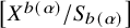 $\left[X^{b(\alpha )}/S_{b(\alpha )}\right]$
as in Examples 3.9 and 3.10.
$\left[X^{b(\alpha )}/S_{b(\alpha )}\right]$
as in Examples 3.9 and 3.10.
As the proof of the main factorization Theorem 3.22 below works entirely on
 $\mathrm {Sym}^{b(\alpha )}(X)$
and on
$\mathrm {Sym}^{b(\alpha )}(X)$
and on
 $\left[X^{b(\alpha )}/S_{b(\alpha )}\right]$
, we get an analogous result in this more general setting. For example, this applies to the following interesting situations:
$\left[X^{b(\alpha )}/S_{b(\alpha )}\right]$
, we get an analogous result in this more general setting. For example, this applies to the following interesting situations:
-
• For f the coarse moduli space of an orbifold, this recovers the above notion of factorization for orbifolds.
-
• For f the crepant resolution of an orbifold, this allows us to factorize generating series indexed by exceptional classes.
-
• For f a fibration, this allows us to factorize generating series indexed by fiber classes.
We plan to explore these applications in future work.
3.2 Plethystic exponentials & generating series
3.2.1 Plethystic exponentials
For an orbifold
 $\mathcal {X}$
with coarse moduli space
$\mathcal {X}$
with coarse moduli space
 $\pi :\mathcal {X}\to X$
, we define two notions of a partition of
$\pi :\mathcal {X}\to X$
, we define two notions of a partition of
 $\alpha $
, which will come up in the statement and proof of Theorem 3.22. One should think of the difference between partitions of an integer n and the set
$\alpha $
, which will come up in the statement and proof of Theorem 3.22. One should think of the difference between partitions of an integer n and the set
 $[n]$
. We denote the set of partitions of the integer n by
$[n]$
. We denote the set of partitions of the integer n by
 $P(n)$
and the set of partitions of the set
$P(n)$
and the set of partitions of the set
 $[n]$
by
$[n]$
by
 $P[n]$
.
$P[n]$
.
Definition 3.14. Given a factorization index set I, an I-partition of
 $\alpha \in I$
is a multiset
$\alpha \in I$
is a multiset
 $\lambda =\{\alpha _1,\dots ,\alpha _k\}\subset I$
, such that
$\lambda =\{\alpha _1,\dots ,\alpha _k\}\subset I$
, such that
 $\sum _i \alpha _i = \alpha $
. We denote the set of I-partitions of
$\sum _i \alpha _i = \alpha $
. We denote the set of I-partitions of
 $\alpha $
by
$\alpha $
by
 $P_I(\alpha )$
or just
$P_I(\alpha )$
or just
 $P(\alpha )$
if the factorization index set is clear. The length of a partition
$P(\alpha )$
if the factorization index set is clear. The length of a partition
 $\lambda =\{\alpha _1,\dots ,\alpha _k\}$
is k. We denote the set of I-partitions of
$\lambda =\{\alpha _1,\dots ,\alpha _k\}$
is k. We denote the set of I-partitions of
 $\alpha $
of length k by
$\alpha $
of length k by
 $P_{I,k}(\alpha )$
.
$P_{I,k}(\alpha )$
.
Definition 3.15. Given
 $\alpha $
, we write
$\alpha $
, we write
 $\alpha =(b(\alpha ),\tilde {\alpha })$
under the splitting
$\alpha =(b(\alpha ),\tilde {\alpha })$
under the splitting
 $\mathrm {N}_0(\mathcal {X})\cong \mathbb {Z}\oplus \widetilde {\mathrm {N}}_0(\mathcal {X})$
from Section 2.2.3. Denote by
$\mathrm {N}_0(\mathcal {X})\cong \mathbb {Z}\oplus \widetilde {\mathrm {N}}_0(\mathcal {X})$
from Section 2.2.3. Denote by
 $[\alpha ]$
the tuple
$[\alpha ]$
the tuple
 $([b(\alpha )],\tilde {\alpha })$
. Given a factorization index set I, an I-partition of
$([b(\alpha )],\tilde {\alpha })$
. Given a factorization index set I, an I-partition of
 $[\alpha ]$
is a collection
$[\alpha ]$
is a collection
 $$ \begin{align*} \{(B_1,\tilde{\alpha}_1), \dots, (B_k,\tilde{\alpha}_k)\}, \end{align*} $$
where
 $B_i\subseteq [b(\alpha )]$
, such that
$B_i\subseteq [b(\alpha )]$
, such that
 $\{B_1,\dots ,B_k\}\in P[b(\alpha )]$
, and
$\{B_1,\dots ,B_k\}\in P[b(\alpha )]$
, and
 $\tilde {\alpha }_i\in \widetilde {\mathrm {N}}_0(\mathcal {X})$
classes such that the collection
$\tilde {\alpha }_i\in \widetilde {\mathrm {N}}_0(\mathcal {X})$
classes such that the collection
 $\{(\left| B_1 \right|,\tilde {\alpha }_1),\dots ,(\left| B_k \right|,\tilde {\alpha }_k)\}$
is an I-partition of
$\{(\left| B_1 \right|,\tilde {\alpha }_1),\dots ,(\left| B_k \right|,\tilde {\alpha }_k)\}$
is an I-partition of
 $\alpha $
in the above sense. Here,
$\alpha $
in the above sense. Here,
 $P[b(\alpha )]$
denotes the set of partitions of the set
$P[b(\alpha )]$
denotes the set of partitions of the set
 $[b(\alpha )]$
.
$[b(\alpha )]$
.
We denote the set of I-partitions of
 $[\alpha ]$
by
$[\alpha ]$
by
 $P_I[\alpha ]$
or just
$P_I[\alpha ]$
or just
 $P[\alpha ]$
if the factorization index set is clear. The length of a partition
$P[\alpha ]$
if the factorization index set is clear. The length of a partition
 $\Xi =\{(B_1,\tilde {\alpha }_1), \dots , (B_k,\tilde {\alpha }_k)\}$
is k.
$\Xi =\{(B_1,\tilde {\alpha }_1), \dots , (B_k,\tilde {\alpha }_k)\}$
is k.
Given an element
 $\Xi =\{(B_1,\tilde {\alpha }_1), \dots , (B_k,\tilde {\alpha }_k)\}$
of
$\Xi =\{(B_1,\tilde {\alpha }_1), \dots , (B_k,\tilde {\alpha }_k)\}$
of
 $P_I[\alpha ]$
, we denote by
$P_I[\alpha ]$
, we denote by
 $B(\Xi )$
the underlying partition
$B(\Xi )$
the underlying partition
 $\{B_1, \dots , B_k\}$
of
$\{B_1, \dots , B_k\}$
of
 $[b(\alpha )]$
.
$[b(\alpha )]$
.
Note that an element
 $\Xi =\{(B_1,\tilde {\alpha }_1), \dots , (B_k,\tilde {\alpha }_k)\}$
of
$\Xi =\{(B_1,\tilde {\alpha }_1), \dots , (B_k,\tilde {\alpha }_k)\}$
of
 $P_I[\alpha ]$
yields an element
$P_I[\alpha ]$
yields an element
 $\left| \Xi \right|=\{(\left| B_1 \right|,\tilde {\alpha }_1),\dots ,(\left| B_k \right|,\tilde {\alpha }_k)\}$
of
$\left| \Xi \right|=\{(\left| B_1 \right|,\tilde {\alpha }_1),\dots ,(\left| B_k \right|,\tilde {\alpha }_k)\}$
of
 $P_I(\alpha )$
by definition. We write
$P_I(\alpha )$
by definition. We write
 $P_I^\lambda [\alpha ]=\{\Xi \in P_I[\alpha ]\ |\ \left| \Xi \right|=\lambda \}$
.
$P_I^\lambda [\alpha ]=\{\Xi \in P_I[\alpha ]\ |\ \left| \Xi \right|=\lambda \}$
.
Now we can define a K-theoretic version of the plethystic exponential. Note that throughout this paper, we consider the K-theory class of a (possibly 2-periodic) complex of sheaves to be the class in
 $K(\mathrm {Coh}(-))$
, rather than one in
$K(\mathrm {Coh}(-))$
, rather than one in
 $K(\mathrm {CoCh}^{(\mathbb {Z}/2)}\mathrm {Coh}(-))$
.
$K(\mathrm {CoCh}^{(\mathbb {Z}/2)}\mathrm {Coh}(-))$
.
Definition 3.16. For
 $\pi :\mathcal {X}\to X$
an orbifold with coarse moduli space and I a factorization index set, let
$\pi :\mathcal {X}\to X$
an orbifold with coarse moduli space and I a factorization index set, let
 $\Xi =\{(B_1,\tilde {\alpha }_1), \dots , (B_k,\tilde {\alpha }_k)\}$
be a partition of
$\Xi =\{(B_1,\tilde {\alpha }_1), \dots , (B_k,\tilde {\alpha }_k)\}$
be a partition of
 $[\alpha ]$
. For each
$[\alpha ]$
. For each
 $\beta \in I$
, let
$\beta \in I$
, let
 $\mathcal {G}_{\beta }$
be an
$\mathcal {G}_{\beta }$
be an
 $S_{b(\beta )}$
-equivariant complex of sheaves on
$S_{b(\beta )}$
-equivariant complex of sheaves on
 $X^{b(\beta )}$
. Assume
$X^{b(\beta )}$
. Assume
 $\Xi $
is ordered such that
$\Xi $
is ordered such that
 $\min (B_1) \leq \dots \leq \min (B_k)$
. We define
$\min (B_1) \leq \dots \leq \min (B_k)$
. We define
 $$ \begin{align*} \mathcal{G}_{\Xi} := \mathcal{G}_{(\left| B_1 \right|,\tilde{\alpha}_1)} \boxtimes \dots \boxtimes \mathcal{G}_{(\left| B_k \right|,\tilde{\alpha}_k)}, \end{align*} $$
as a complex of sheaves on
 $X^{b(\alpha )}$
, where each pullback is along the map
$X^{b(\alpha )}$
, where each pullback is along the map
 $\mathrm {pr}_{b_i^1,\dots ,b_i^{l_i}}:X^{b(\alpha )} \to X^{\left| B_i \right|}$
specified by the subset
$\mathrm {pr}_{b_i^1,\dots ,b_i^{l_i}}:X^{b(\alpha )} \to X^{\left| B_i \right|}$
specified by the subset
 $B_i=\{b_i^1,\dots ,b_i^{l_i}\}$
, where we order
$B_i=\{b_i^1,\dots ,b_i^{l_i}\}$
, where we order
 $B_i$
such that
$B_i$
such that
 $b_i^1<\dots <b_i^{l_i}$
.
$b_i^1<\dots <b_i^{l_i}$
.
For a partition
 $\lambda \in P(\alpha )$
of
$\lambda \in P(\alpha )$
of
 $\alpha $
, we define the complex of sheaves on
$\alpha $
, we define the complex of sheaves on
 $X^{b(\alpha )}$
 $$ \begin{align*} \mathcal{G}_\lambda := \bigoplus_{\Xi\in P^\lambda[\alpha]} \mathcal{G}_{\Xi}, \end{align*} $$
which inherits a natural
 $S_{b(\alpha )}$
-equivariant structure, as
$S_{b(\alpha )}$
-equivariant structure, as
 $S_{b(\alpha )}$
permutes the various projections
$S_{b(\alpha )}$
permutes the various projections
 $X^{b(\alpha )} \to X^{\left| B_i \right|}$
by permuting the partitions
$X^{b(\alpha )} \to X^{\left| B_i \right|}$
by permuting the partitions
 $\{B_i\}_i$
of
$\{B_i\}_i$
of
 $[b(\alpha )]$
realizing the partition
$[b(\alpha )]$
realizing the partition
 $\{\left| B_i \right|\}_i$
of
$\{\left| B_i \right|\}_i$
of
 $b(\alpha )$
. For compatibility with constructions in Section 3.3.3, the equivariant structure involves an additional sign. We will explain this sign and details about the equivariant structure in more generality in Definition 3.31.
$b(\alpha )$
. For compatibility with constructions in Section 3.3.3, the equivariant structure involves an additional sign. We will explain this sign and details about the equivariant structure in more generality in Definition 3.31.
Analogously, we make the following definition on the symmetric product.
Definition 3.17. For each
 $\beta \in I$
, let
$\beta \in I$
, let
 $\mathcal {G}_{\beta }$
be a complex of sheaves on
$\mathcal {G}_{\beta }$
be a complex of sheaves on
 $\mathrm {Sym}^{b(\alpha )}(X)$
. Let
$\mathrm {Sym}^{b(\alpha )}(X)$
. Let
 $\lambda =\{\alpha _1,\dots ,\alpha _k\}$
in
$\lambda =\{\alpha _1,\dots ,\alpha _k\}$
in
 $P(\alpha )$
be a partition of
$P(\alpha )$
be a partition of
 $\alpha $
. Take a partition
$\alpha $
. Take a partition
 $\Xi =\{(B_1,\tilde {\alpha }_1), \dots , (B_k,\tilde {\alpha }_k)\}$
in
$\Xi =\{(B_1,\tilde {\alpha }_1), \dots , (B_k,\tilde {\alpha }_k)\}$
in
 $P^\lambda [\alpha ]$
. Assume
$P^\lambda [\alpha ]$
. Assume
 $\Xi $
is ordered such that
$\Xi $
is ordered such that
 $\min (B_1) \leq \dots \leq \min (B_k)$
. Set
$\min (B_1) \leq \dots \leq \min (B_k)$
. Set
 $$ \begin{align*} \mathcal{G}_{\Xi} := \mathcal{G}_{(\left| B_1 \right|,\tilde{\alpha}_1)} \boxtimes \dots \boxtimes \mathcal{G}_{(\left| B_k \right|,\tilde{\alpha}_k)}, \end{align*} $$
as a complex of sheaves on
 $\prod _{i=1}^k\mathrm {Sym}^{\left| B_i \right|}(X)$
. Take
$\prod _{i=1}^k\mathrm {Sym}^{\left| B_i \right|}(X)$
. Take
 $S^B_\lambda $
to be the group
$S^B_\lambda $
to be the group
 $\prod _i S_{l_i}$
, where
$\prod _i S_{l_i}$
, where
 $l_i$
is the number of occurrences of
$l_i$
is the number of occurrences of
 $\alpha _i$
in
$\alpha _i$
in
 $\lambda $
. It acts on
$\lambda $
. It acts on
 $\prod _{i=1}^k\mathrm {Sym}^{\left| B_i \right|}(X)$
by permuting the blocks
$\prod _{i=1}^k\mathrm {Sym}^{\left| B_i \right|}(X)$
by permuting the blocks
 $\mathrm {Sym}^{\left| B_i \right|}(X)$
with the same
$\mathrm {Sym}^{\left| B_i \right|}(X)$
with the same
 $\alpha _i$
.
$\alpha _i$
.
 $\mathcal {G}_{\Xi }$
carries a natural
$\mathcal {G}_{\Xi }$
carries a natural
 $S^B_\lambda $
-equivariant structure. We have the composition of morphisms
$S^B_\lambda $
-equivariant structure. We have the composition of morphisms
 $$ \begin{align*} \vartheta: \left[\left(\prod_{i=1}^k\mathrm{Sym}^{\left| B_i \right|}(X)\right)/S^B_\lambda\right] \to \prod_{\alpha_i\in \lambda} \mathrm{Sym}^{l_i}\left(\mathrm{Sym}^{b(\alpha_i)}(X)\right) \to \mathrm{Sym}^{b(\alpha)}(X), \end{align*} $$
where the product in the second term goes over every
 $\alpha _i$
in
$\alpha _i$
in
 $\lambda $
viewed as a set instead of a multiset, the first morphism is the coarse space, and the second morphism adds up the different points in X. Set
$\lambda $
viewed as a set instead of a multiset, the first morphism is the coarse space, and the second morphism adds up the different points in X. Set
We will see in Lemma 3.18(b) below that the construction of
 $\mathcal {G}_\lambda $
is independent of the choice of
$\mathcal {G}_\lambda $
is independent of the choice of
 $\Xi $
.
$\Xi $
.
We now show some important compatibilities and properties of the previous two constructions.
Lemma 3.18. For each
 $\beta \in I$
, let
$\beta \in I$
, let
 $\mathcal {G}_{\beta }$
be a complex of sheaves on
$\mathcal {G}_{\beta }$
be a complex of sheaves on
 $\mathrm {Sym}^{b(\alpha )}(X)$
, and let
$\mathrm {Sym}^{b(\alpha )}(X)$
, and let
 $\mathcal {E}_{\beta }$
be an
$\mathcal {E}_{\beta }$
be an
 $S_{b(\beta )}$
-equivariant complex of sheaves on
$S_{b(\beta )}$
-equivariant complex of sheaves on
 $X^{b(\beta )}$
. Let
$X^{b(\beta )}$
. Let
 $\lambda =\{\alpha _1,\dots ,\alpha _k\}$
in
$\lambda =\{\alpha _1,\dots ,\alpha _k\}$
in
 $P(\alpha )$
be a partition of
$P(\alpha )$
be a partition of
 $\alpha $
. By abuse of notation, denote the quotient morphism
$\alpha $
. By abuse of notation, denote the quotient morphism
 $[X^n/S_n]\to \mathrm {Sym}^n(X)$
by p for every n. Then
$[X^n/S_n]\to \mathrm {Sym}^n(X)$
by p for every n. Then
-
(a)
$p_*\left(\mathcal {E}_\lambda \right)\cong \left(p_*\mathcal {E}\right)_\lambda $
, -
(b)
$\mathcal {G}_\lambda \cong p_*\left((p^*\mathcal {G})_\lambda \right)$
, -
(c)
$p_*\left(\mathcal {E}_\lambda \right)\cong p_*\left((p^*p_*\mathcal {E})_\lambda \right)$
, and -
(d) the operation
$\left\{\mathcal {G}_\beta \right\}\mapsto \mathcal {G}_\lambda $
descends to K-theory.


Proof. Note first that the coarse space p satisfies that the adjunction
 $p_*p^*\cong \mathrm {id}$
is a natural isomorphism. Assuming (a), we show (b), (c), and (d). For (b), we see
$p_*p^*\cong \mathrm {id}$
is a natural isomorphism. Assuming (a), we show (b), (c), and (d). For (b), we see
 $$ \begin{align*} p_*\left((p^*\mathcal{G})_\lambda\right) \cong \left(p_*p^*\mathcal{G}\right)_\lambda \cong \mathcal{G}_\lambda, \end{align*} $$
where we first use (a) and then the adjunction isomorphism. For (c), we see
 $$ \begin{align*} p_*\left((p^*p_*\mathcal{E})_\lambda\right) \cong \left(p_*p^*p_*\mathcal{E}\right)_\lambda \cong \left(p_*\mathcal{E}\right)_\lambda \cong p_*\left(\mathcal{E}_\lambda\right), \end{align*} $$
where we first use (a), then the adjunction isomorphism, and then (a) again. For (d), note that the construction of
 $\mathcal {G}_\lambda $
in Definition 3.17 involves only pullbacks along flat morphisms and a pushforward along
$\mathcal {G}_\lambda $
in Definition 3.17 involves only pullbacks along flat morphisms and a pushforward along
 $\vartheta $
, which is the composition of a finite morphism and a proper coarse moduli space, making
$\vartheta $
, which is the composition of a finite morphism and a proper coarse moduli space, making
 $\vartheta _*$
exact. Hence, the operation
$\vartheta _*$
exact. Hence, the operation
 $\left\{\mathcal {G}_\alpha \right\}\mapsto \mathcal {G}_\lambda $
descends to K-theory.
$\left\{\mathcal {G}_\alpha \right\}\mapsto \mathcal {G}_\lambda $
descends to K-theory.
It remains to prove (a). Take
 $\Xi =\{(B_1,\tilde {\alpha }_1), \dots , (B_k,\tilde {\alpha }_k)\}$
in
$\Xi =\{(B_1,\tilde {\alpha }_1), \dots , (B_k,\tilde {\alpha }_k)\}$
in
 $P^\lambda [\alpha ]$
and assume
$P^\lambda [\alpha ]$
and assume
 $\Xi $
is ordered such that
$\Xi $
is ordered such that
 $\min (B_1) \leq \dots \leq \min (B_k)$
. Consider
$\min (B_1) \leq \dots \leq \min (B_k)$
. Consider
 $\mathcal {E}_\Xi $
on
$\mathcal {E}_\Xi $
on
 $X^{b(\alpha )}$
. It comes with a natural
$X^{b(\alpha )}$
. It comes with a natural
 $\prod _i S_{b(\alpha _i)}$
-equivariant structure, where
$\prod _i S_{b(\alpha _i)}$
-equivariant structure, where
 $\prod _i S_{b(\alpha _i)}$
acts on
$\prod _i S_{b(\alpha _i)}$
acts on
 $X^{b(\alpha )}$
by permuting the indices within the blocks indexed by the
$X^{b(\alpha )}$
by permuting the indices within the blocks indexed by the
 $B_i$
. As in Definition 3.17
$B_i$
. As in Definition 3.17
 $S^B_\lambda $
acts on
$S^B_\lambda $
acts on
 $X^{b(\alpha )}$
by permuting entire blocks with indices
$X^{b(\alpha )}$
by permuting entire blocks with indices
 $B_i$
and
$B_i$
and
 $B_j$
with
$B_j$
with
 $\alpha _i=\alpha _j$
. Define the subgroup
$\alpha _i=\alpha _j$
. Define the subgroup
 $$ \begin{align*} S_\Xi \subseteq S_{b(\alpha)} \end{align*} $$
to be the subgroup of
 $S_{b(\alpha )}$
fixing the partition
$S_{b(\alpha )}$
fixing the partition
 $\Xi $
.
$\Xi $
.
 $\mathcal {E}_\Xi $
comes with a natural
$\mathcal {E}_\Xi $
comes with a natural
 $S_\Xi $
-equivariant structure. We can identify this group as
$S_\Xi $
-equivariant structure. We can identify this group as
 $$ \begin{align*} S_\Xi = \left(\textstyle\prod_i S_{b(\alpha_i)}\right)\rtimes S^B_\lambda. \end{align*} $$
By Proposition A.1, the inclusion of
 $S_\Xi $
in
$S_\Xi $
in
 $S_{b(\alpha )}$
gives us a morphism
$S_{b(\alpha )}$
gives us a morphism
 $q_\Xi :\left[X^{b(\alpha )}/S_\Xi \right]\to \left[X^{b(\alpha )}/S_{b(\alpha )}\right]$
. We have a bijection
$q_\Xi :\left[X^{b(\alpha )}/S_\Xi \right]\to \left[X^{b(\alpha )}/S_{b(\alpha )}\right]$
. We have a bijection
 $S_{b(\alpha )}/S_\Xi \xrightarrow {\sim }P^\lambda (\alpha )$
given by
$S_{b(\alpha )}/S_\Xi \xrightarrow {\sim }P^\lambda (\alpha )$
given by
 $[\sigma ]\mapsto \sigma (\Xi )$
, which together with Proposition A.2 gives us an isomorphism
$[\sigma ]\mapsto \sigma (\Xi )$
, which together with Proposition A.2 gives us an isomorphism
 $$ \begin{align} \left(q_\Xi\right)_* \mathcal{E}_\Xi \cong \mathcal{E}_\lambda. \end{align} $$
Details about the equivariant structures are explained in Remark 3.32 after the equivariant structure of
 $\bar {\mathcal {G}}_\lambda $
is introduced in detail in Definition 3.31. Consider the commutative diagram
$\bar {\mathcal {G}}_\lambda $
is introduced in detail in Definition 3.31. Consider the commutative diagram

This gives us
 $$ \begin{align*} p_*\left(\mathcal{E}_\lambda\right) \cong p_*\left(q_\Xi\right)_*\left(\mathcal{E}_\Xi\right)\cong \vartheta_*\left(\textstyle\prod_i p\right)_*\left(\mathcal{E}_\Xi\right). \end{align*} $$
But by construction
 $\left(\textstyle \prod _i p\right)_*\left(\mathcal {E}_\Xi \right)$
is the same as
$\left(\textstyle \prod _i p\right)_*\left(\mathcal {E}_\Xi \right)$
is the same as
 $\left(p_*\mathcal {E}\right)_\Xi $
, finishing the proof of (a).
$\left(p_*\mathcal {E}\right)_\Xi $
, finishing the proof of (a).
Using the pieces in Definitions 3.16 and 3.17, together with Lemma 3.18(d), we can now define plethystic exponentials in K-theory.
Definition 3.19. Given a factorization index set I, for a system
 $\mathcal {G}_{\alpha }$
of
$\mathcal {G}_{\alpha }$
of
 $S_{b(\alpha )}$
-equivariant complexes of sheaves on
$S_{b(\alpha )}$
-equivariant complexes of sheaves on
 $X^{b(\alpha )}$
, we define the plethystic exponential to be
$X^{b(\alpha )}$
, we define the plethystic exponential to be
 $$ \begin{align*} \mathrm{PExp}^I\left(\sum_{\alpha\in I}q^{\alpha} [\mathcal{G}_{\alpha}]\right) := 1+ \sum_{\alpha\in I} q^{\alpha} \sum_{\lambda\in P(\alpha)} [\mathcal{G}_\lambda], \end{align*} $$
where
 $1$
denotes the unit in the K-theory of
$1$
denotes the unit in the K-theory of
 $X^0=\mathrm {pt}$
.
$X^0=\mathrm {pt}$
.
For a system
 $\mathcal {G}_{\alpha }$
of complexes of sheaves on
$\mathcal {G}_{\alpha }$
of complexes of sheaves on
 $\mathrm {Sym}^{b(\alpha )}(X)$
, we define the plethystic exponential to be
$\mathrm {Sym}^{b(\alpha )}(X)$
, we define the plethystic exponential to be
 $$ \begin{align*} \mathrm{PExp}^I\left(\sum_{\alpha\in I}q^{\alpha} [\mathcal{G}_{\alpha}]\right) := p_\ast\mathrm{PExp}^I\left(\sum_{\alpha\in I}q^{\alpha} [p^*\mathcal{G}_{\alpha}]\right), \end{align*} $$
where
 $p:[X^{b(\alpha )}/S_{b(\alpha )}] \to \mathrm {Sym}^{b(\alpha )}(X)$
denotes the quotient morphism. Here we use Lemma 3.18(d) for well-definedness in K-theory.
$p:[X^{b(\alpha )}/S_{b(\alpha )}] \to \mathrm {Sym}^{b(\alpha )}(X)$
denotes the quotient morphism. Here we use Lemma 3.18(d) for well-definedness in K-theory.
For a system
 $\mathcal {G}_{\alpha }$
of complexes of sheaves on X, we define the plethystic exponential to be
$\mathcal {G}_{\alpha }$
of complexes of sheaves on X, we define the plethystic exponential to be
 $$ \begin{align*} \mathrm{PExp}^I\left(\sum_{\alpha\in I}q^{\alpha} [\mathcal{G}_{\alpha}]\right) := \mathrm{PExp}^I\left(\sum_{\alpha\in I}q^{\alpha} [i_\ast\mathcal{G}_{\alpha}]\right), \end{align*} $$
where
 $i:X \to \mathrm {Sym}^{b(\alpha )}(X)$
denotes the diagonal embedding.
$i:X \to \mathrm {Sym}^{b(\alpha )}(X)$
denotes the diagonal embedding.
The plethystic exponential defined above can in general depend on I, which is reflected in the notation
 $\mathrm {PExp}^I$
. Recall that [Reference Okounkov31] defines the plethystic exponential instead using the operation
$\mathrm {PExp}^I$
. Recall that [Reference Okounkov31] defines the plethystic exponential instead using the operation
 $\mathsf {S}^\bullet $
, which is the morphism in K-theory induced by the symmetric product of vector spaces. We will now show the relation between our definition and the one in [Reference Okounkov31]. If the factorization index set I is closed under addition, as is the case for schemes, the definitions agree, and, by abuse of notation, we will sometimes write
$\mathsf {S}^\bullet $
, which is the morphism in K-theory induced by the symmetric product of vector spaces. We will now show the relation between our definition and the one in [Reference Okounkov31]. If the factorization index set I is closed under addition, as is the case for schemes, the definitions agree, and, by abuse of notation, we will sometimes write
 $\mathrm {PExp}$
for the function
$\mathrm {PExp}$
for the function
 $\mathsf {S}^\bullet $
below.
$\mathsf {S}^\bullet $
below.
Lemma 3.20. For a system
 $\mathcal {G}_{\alpha }$
of complexes of sheaves on
$\mathcal {G}_{\alpha }$
of complexes of sheaves on
 $\mathrm {Sym}^{b(\alpha )}(X)$
, we have
$\mathrm {Sym}^{b(\alpha )}(X)$
, we have
 $$ \begin{align*} \chi\left(\mathrm{PExp}^I\left(\sum_{\alpha\in I}q^\alpha [\mathcal{G}_\alpha]\right)\right)= \left.{\mathsf{S}^\bullet\left(\sum_{\alpha\in I}q^\alpha \chi\left([\mathcal{G}_\alpha]\right)\right)}\right\vert_{I}, \end{align*} $$
where
 $\left.{-}\right\vert _{I}$
restricts the right-hand side to all terms
$\left.{-}\right\vert _{I}$
restricts the right-hand side to all terms
 $(\cdots )q^\alpha $
with
$(\cdots )q^\alpha $
with
 $\alpha \in I$
. For I closed under addition, for example, in the scheme case of Lemma 3.3, the restriction
$\alpha \in I$
. For I closed under addition, for example, in the scheme case of Lemma 3.3, the restriction
 $\left.{-}\right\vert _{I}$
is not necessary. In particular, in this case
$\left.{-}\right\vert _{I}$
is not necessary. In particular, in this case
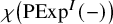 $\chi \left(\mathrm {PExp}^I\left(-\right)\right)$
is multiplicative under addition of the argument.
$\chi \left(\mathrm {PExp}^I\left(-\right)\right)$
is multiplicative under addition of the argument.
Corollary 3.21. In the
 $\mathsf {T}=(\mathbb {C}^*)^3$
-equivariant case, the identification in Lemma 3.20 above gives us the explicit computational formula
$\mathsf {T}=(\mathbb {C}^*)^3$
-equivariant case, the identification in Lemma 3.20 above gives us the explicit computational formula
 $$ \begin{align*} \chi_{\mathsf{T}}\left(\mathrm{PExp}^I\left(\sum_{\alpha\in I}q^\alpha [\mathcal{G}_\alpha]\right)\right)= \left.{\exp\left(\sum_{n>0}\frac{1}{n}\sum_{\alpha\in I}q^{n\alpha}\chi_{\mathsf{T}}([\mathcal{G}_\alpha],t_1^n,t_2^n,t_3^n)\right)}\right\vert_{I}, \end{align*} $$
where
 $t_1,t_2,t_3$
is a basis for the characters of
$t_1,t_2,t_3$
is a basis for the characters of
 $\mathsf {T}$
.
$\mathsf {T}$
.
Proof of Lemma 3.20
Take
 $\alpha \in I$
,
$\alpha \in I$
,
 $\lambda =\{\alpha _1,\dots ,\alpha _k\}$
in
$\lambda =\{\alpha _1,\dots ,\alpha _k\}$
in
 $P(\alpha )$
, and
$P(\alpha )$
, and
 $\Xi \in P^\lambda [\alpha ]$
. By invariance of Euler characteristics under pushforward and Lemma 3.18 (b), we obtain the identity
$\Xi \in P^\lambda [\alpha ]$
. By invariance of Euler characteristics under pushforward and Lemma 3.18 (b), we obtain the identity
 $$ \begin{align} \chi\left(\mathrm{PExp}^I\left(\sum_{\alpha\in I}q^\alpha [\mathcal{G}_\alpha]\right)\right)= 1+ \sum_{\alpha\in I} q^{\alpha} \sum_{\lambda\in P(\alpha)} \chi\left(\left[\left(\textstyle\prod_i \mathrm{Sym}^{b(\alpha_i)}(X)\right)/S^B_\lambda\right],\mathcal{G}_\Xi\right), \end{align} $$
where we have chosen a representative
 $\Xi $
for every
$\Xi $
for every
 $\lambda $
.
$\lambda $
.
The coefficient of
 $q^\alpha $
in
$q^\alpha $
in
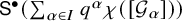 $\mathsf {S}^\bullet \left(\sum _{\alpha \in I}q^\alpha \chi \left([\mathcal {G}_\alpha ]\right)\right)$
is
$\mathsf {S}^\bullet \left(\sum _{\alpha \in I}q^\alpha \chi \left([\mathcal {G}_\alpha ]\right)\right)$
is
 $$ \begin{align*} \sum_{\lambda\in P(\alpha)}\left(\textstyle\prod_i \chi\left(\mathcal{G}_{\alpha_i}\right)\right)^{S_\lambda^B}, \end{align*} $$
where we have again chosen a representative
 $\Xi \in P^\lambda (\alpha )$
which determines the order of the product. As above,
$\Xi \in P^\lambda (\alpha )$
which determines the order of the product. As above,
 $S_\lambda ^B$
acts by permuting the various multiples of the same factors and we take the
$S_\lambda ^B$
acts by permuting the various multiples of the same factors and we take the
 $S_\lambda ^B$
-invariant part. Evaluating the Euler characteristics in the right-hand side of (15) is the same as taking the
$S_\lambda ^B$
-invariant part. Evaluating the Euler characteristics in the right-hand side of (15) is the same as taking the
 $S_\lambda ^B$
-invariant part of the pushforward of the class of
$S_\lambda ^B$
-invariant part of the pushforward of the class of
 $\mathcal {G}_\Xi $
to
$\mathcal {G}_\Xi $
to
 $BS_\lambda ^B$
. Summing over
$BS_\lambda ^B$
. Summing over
 $\lambda \in P(\alpha )$
, this yields exactly the terms of
$\lambda \in P(\alpha )$
, this yields exactly the terms of
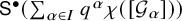 $\mathsf {S}^\bullet \left(\sum _{\alpha \in I}q^\alpha \chi \left([\mathcal {G}_\alpha ]\right)\right)$
above, proving the first identification.
$\mathsf {S}^\bullet \left(\sum _{\alpha \in I}q^\alpha \chi \left([\mathcal {G}_\alpha ]\right)\right)$
above, proving the first identification.
We can now use that both sides behave the same under addition of arguments. So, we may assume all
 $\chi \left([\mathcal {G}_\alpha ]\right)$
are simply characters
$\chi \left([\mathcal {G}_\alpha ]\right)$
are simply characters
 $\mathbf {t}^{\boldsymbol {\mu }_\alpha }$
. Then we have by definition
$\mathbf {t}^{\boldsymbol {\mu }_\alpha }$
. Then we have by definition
 $$ \begin{align*} \chi\left(\mathrm{PExp}^I\left(\sum_{\alpha\in I}q^\alpha [\mathcal{G}_\alpha]\right)\right) = 1+ \sum_{\alpha\in I} q^\alpha \sum_{\lambda\in P(\alpha)} \mathbf{t}^{\sum_{\alpha_i\in \lambda}\boldsymbol{\mu}_{\alpha_i}}. \end{align*} $$
We can rewrite this sum as
 $$ \begin{align*} \left.{\prod_{\alpha\in I} \left(\sum_{k\geq 0} \left(q^\alpha \mathbf{t}^{\boldsymbol{\mu}_{\alpha}}\right)^k\right)}\right\vert_{I} = \left.{\prod_{\alpha\in I} \left(1-q^\alpha \mathbf{t}^{\boldsymbol{\mu}_\alpha}\right)^{-1}}\right\vert_{I}, \end{align*} $$
where we identified the geometric series. The formal power series of the logarithm now allows us to rewrite this in the desired form.
 $$ \begin{align*} \chi\left(\mathrm{PExp}^I\left(\sum_{\alpha\in I}q^\alpha [\mathcal{G}_\alpha]\right)\right) = \left.{\exp\left(\sum_{n>0}\frac{1}{n}\sum_{\alpha\in I}q^{n\alpha} \mathbf{t}^{n \boldsymbol{\mu}_\alpha}\right)}\right\vert_{I}. \end{align*} $$
3.2.2 Factorization theorem
Now we can state the main result of this section.
Theorem 3.22. Let
 $\mathcal {X}$
be an orbifold with coarse moduli space
$\mathcal {X}$
be an orbifold with coarse moduli space
 $\pi :\mathcal {X}\to X$
and let I be a factorization index semigroup. For a factorizable system
$\pi :\mathcal {X}\to X$
and let I be a factorization index semigroup. For a factorizable system
 $\mathcal {F}_{\alpha }$
on
$\mathcal {F}_{\alpha }$
on
 $\mathrm {Sym}^{b(\alpha )}(X)$
, there exist classes
$\mathrm {Sym}^{b(\alpha )}(X)$
, there exist classes
 $[\mathcal {G}_{\alpha }]$
on X such that
$[\mathcal {G}_{\alpha }]$
on X such that
 $$ \begin{align*} 1 + \sum_{\alpha\in I} q^{\alpha} [\mathcal{F}_{\alpha}] = \mathrm{PExp}^I\left(\sum_{\alpha\in I}q^{\alpha} [\mathcal{G}_{\alpha}]\right) \end{align*} $$
in
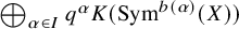 $\bigoplus _{\alpha \in I}q^\alpha K(\mathrm {Sym}^{b(\alpha )}(X))$
.
$\bigoplus _{\alpha \in I}q^\alpha K(\mathrm {Sym}^{b(\alpha )}(X))$
.
Let U be the nonstacky locus, and let S be its complement in X. If the system is given such that for any
 $\alpha \in I\setminus \Delta _I$
,
$\alpha \in I\setminus \Delta _I$
,
 $\left.{\mathcal {F}_{\alpha }}\right\vert _{\mathrm {Sym}^{b(\alpha )}(U)}=0$
, then the classes
$\left.{\mathcal {F}_{\alpha }}\right\vert _{\mathrm {Sym}^{b(\alpha )}(U)}=0$
, then the classes
 $[\mathcal {G}_{\alpha }]$
can be chosen so that they are supported on
$[\mathcal {G}_{\alpha }]$
can be chosen so that they are supported on
 $S\subset X$
for
$S\subset X$
for
 $\alpha \in I\setminus \Delta _I$
.
$\alpha \in I\setminus \Delta _I$
.
The second case of the theorem is fulfilled for pushforwards of virtual structure sheaves from the Hilbert scheme, which is our main application.
Remark 3.23. Note we require I to be closed under addition. The dependence on this condition is subtle, and we plan to study the necessary corrections to the above Theorem to make it work with I that are not closed under addition.
Remark 3.24. The last part of the above theorem would work for any subset that is closed under addition instead of
 $\Delta _I$
and any subscheme of X.
$\Delta _I$
and any subscheme of X.
By applying Euler characteristics on both sides, we obtain the following computational formula, which can be combined with Lemma 3.20 to compute the left-hand side in simpler terms.
Corollary 3.25. In the setting of Theorem 3.22 above, for a factorizable system
 $\mathcal {F}_{\alpha }$
on
$\mathcal {F}_{\alpha }$
on
 $\mathrm {Sym}^{b(\alpha )}(X)$
, there exist classes
$\mathrm {Sym}^{b(\alpha )}(X)$
, there exist classes
 $[\mathcal {G}_{\alpha }]$
on X such that
$[\mathcal {G}_{\alpha }]$
on X such that
 $$ \begin{align*} 1 + \sum_{\alpha\in I} q^{\alpha} \chi\left(\mathrm{Sym}^{b(\alpha)}(X),\mathcal{F}_{\alpha}\right) = \mathrm{PExp}^I\left(\sum_{\alpha\in I}q^{\alpha} \chi(X,\mathcal{G}_{\alpha})\right), \end{align*} $$
where the right-hand side can be computed using Lemma 3.20.
As in Theorem 3.22 above, if the system is given such that for any
 $\alpha \in I\setminus \Delta _I$
,
$\alpha \in I\setminus \Delta _I$
,
 $\left.{\mathcal {F}_{\alpha }}\right\vert _{\mathrm {Sym}^{b(\alpha )}(U)}$
vanishes, then the classes
$\left.{\mathcal {F}_{\alpha }}\right\vert _{\mathrm {Sym}^{b(\alpha )}(U)}$
vanishes, then the classes
 $[\mathcal {G}_{\alpha }]$
can be chosen so that they are supported on
$[\mathcal {G}_{\alpha }]$
can be chosen so that they are supported on
 $S\subset X$
for
$S\subset X$
for
 $\alpha \in I\setminus \Delta _I$
.
$\alpha \in I\setminus \Delta _I$
.
3.3 Proof of Theorem 3.22
The proof will work with an
 $S_{b(\alpha )}$
-equivariant factorizable system on
$S_{b(\alpha )}$
-equivariant factorizable system on
 $X^{b(\alpha )}$
. By Lemma 3.11 and Example 3.13, a factorizable system on
$X^{b(\alpha )}$
. By Lemma 3.11 and Example 3.13, a factorizable system on
 $\mathrm {Sym}^{b(\alpha )}(X)$
gives this by pullback. For the entire proof, we fix an orbifold
$\mathrm {Sym}^{b(\alpha )}(X)$
gives this by pullback. For the entire proof, we fix an orbifold
 $\mathcal {X}$
with coarse space
$\mathcal {X}$
with coarse space
 $\pi :\mathcal {X}\to X$
and a factorization index semigroup I. As the factorization index semigroup is fixed, we suppress it from the notation whenever reasonable.
$\pi :\mathcal {X}\to X$
and a factorization index semigroup I. As the factorization index semigroup is fixed, we suppress it from the notation whenever reasonable.
3.3.1 K-theory class
The (2-periodic) complexes of sheaves of the given factorizable system
 $\mathcal {F}_\alpha $
factor into simpler parts according to partitions of
$\mathcal {F}_\alpha $
factor into simpler parts according to partitions of
 $\alpha $
. Roughly, the
$\alpha $
. Roughly, the
 $\mathcal {G}_\alpha $
are defined as (double) complexes tracking the possible splittings of
$\mathcal {G}_\alpha $
are defined as (double) complexes tracking the possible splittings of
 $\alpha $
into smaller parts by systems of subordinate partitions. For now, we will only define the complexes
$\alpha $
into smaller parts by systems of subordinate partitions. For now, we will only define the complexes
 $\mathcal {G}_\alpha $
with trivial differential and examine their K-theory classes. Later in Section 3.3.3, we will introduce a nontrivial differential and use that K-theory classes are independent of the differential.
$\mathcal {G}_\alpha $
with trivial differential and examine their K-theory classes. Later in Section 3.3.3, we will introduce a nontrivial differential and use that K-theory classes are independent of the differential.
To keep track of the different ways to split
 $[\alpha ]$
into smaller parts by different partitions, we use the following notion of an
$[\alpha ]$
into smaller parts by different partitions, we use the following notion of an
 $\alpha $
-index tree.
$\alpha $
-index tree.
Definition 3.26. With I the fixed factorization index semigroup, and
 $\alpha \in I$
, an
$\alpha \in I$
, an
 $\alpha $
-index tree is a rooted tree, with each nonleaf having at least two children, together with a tuple
$\alpha $
-index tree is a rooted tree, with each nonleaf having at least two children, together with a tuple
 $(B_l,\tilde {\alpha }_l)$
for every leaf l such that
$(B_l,\tilde {\alpha }_l)$
for every leaf l such that
 $\{(B_l,\tilde {\alpha }_l)\ |\ l\ \mathrm {leaf}\}$
is an I-partition of
$\{(B_l,\tilde {\alpha }_l)\ |\ l\ \mathrm {leaf}\}$
is an I-partition of
 $[\alpha ]$
. We denote the set of all
$[\alpha ]$
. We denote the set of all
 $\alpha $
-index trees by
$\alpha $
-index trees by
 $\mathcal {T}(\alpha )$
, and we denote the set of
$\mathcal {T}(\alpha )$
, and we denote the set of
 $\alpha $
-index trees with exactly k nonleaf nodes by
$\alpha $
-index trees with exactly k nonleaf nodes by
 $\mathcal {T}(\alpha ,k)$
.
$\mathcal {T}(\alpha ,k)$
.
For every node v, we set
 $B_v$
to be the union of all
$B_v$
to be the union of all
 $B_l$
with l a leaf descendant of v. Similarly, we set
$B_l$
with l a leaf descendant of v. Similarly, we set
 $\tilde {\alpha }_v$
to be the sum of all
$\tilde {\alpha }_v$
to be the sum of all
 $\tilde {\alpha }_l$
with l a leaf descendant of v.
$\tilde {\alpha }_l$
with l a leaf descendant of v.
Given a partition
 $\Xi =\{(B_1,\tilde {\alpha }_1), \dots , (B_k,\tilde {\alpha }_k)\}$
of
$\Xi =\{(B_1,\tilde {\alpha }_1), \dots , (B_k,\tilde {\alpha }_k)\}$
of
 $[\alpha ]$
, we denote by
$[\alpha ]$
, we denote by
 $\mathcal {T}_\Xi (\alpha )$
the set of
$\mathcal {T}_\Xi (\alpha )$
the set of
 $\alpha $
-index trees with partition
$\alpha $
-index trees with partition
 $\Xi $
at the level of root children.
$\Xi $
at the level of root children.
For several constructions we need a specified ordering on the index tree or on a given partition of
 $[\alpha ]$
.
$[\alpha ]$
.
Definition 3.27. An ordering of an
 $\alpha $
-index tree is a total order on its set of nodes, compatible with the tree structure in the following way. If v is a descendant of w, then we require
$\alpha $
-index tree is a total order on its set of nodes, compatible with the tree structure in the following way. If v is a descendant of w, then we require
 $v \leq w$
, and if
$v \leq w$
, and if
 $v_1$
and
$v_1$
and
 $v_2$
are siblings with
$v_2$
are siblings with
 $v_1 < v_2$
, then we require all descendants of
$v_1 < v_2$
, then we require all descendants of
 $v_1$
to be smaller than all descendants of
$v_1$
to be smaller than all descendants of
 $v_2$
.
$v_2$
.
Definition 3.28. Let
 $\leq _1, \leq _2$
be two orderings on an index tree T. Order the relevant nodes of T such that
$\leq _1, \leq _2$
be two orderings on an index tree T. Order the relevant nodes of T such that
 $v_1 <_1 \cdots <_1 v_k$
. There is a unique
$v_1 <_1 \cdots <_1 v_k$
. There is a unique
 $\sigma \in S_k$
such that
$\sigma \in S_k$
such that
 $v_{\sigma (1)} <_2 \cdots <_2 v_{\sigma (k)}$
(the one defined by exactly this condition). We define
$v_{\sigma (1)} <_2 \cdots <_2 v_{\sigma (k)}$
(the one defined by exactly this condition). We define
 $s(\leq _1,\leq _2)=\mathrm {sgn}(\sigma )$
.
$s(\leq _1,\leq _2)=\mathrm {sgn}(\sigma )$
.
Definition 3.29. The standard ordering of an
 $\alpha $
-index tree T, which we denote by
$\alpha $
-index tree T, which we denote by
 $\leq _T$
, is defined recursively as follows. Take the root and make it the unique maximal node. Order the root children
$\leq _T$
, is defined recursively as follows. Take the root and make it the unique maximal node. Order the root children
 $\{v_1,\dots ,v_k\}$
by
$\{v_1,\dots ,v_k\}$
by
 $$ \begin{align*} v_i \leq_T v_j :\Leftrightarrow \min(B_{v_i}) \leq \min(B_{v_j}). \end{align*} $$
For each root child
 $v_i$
, order all its descendants recursively as above (pretending that
$v_i$
, order all its descendants recursively as above (pretending that
 $v_i$
is the root node). Finally for any pair of root children
$v_i$
is the root node). Finally for any pair of root children
 $v_i \leq _T v_j$
order all descendants of
$v_i \leq _T v_j$
order all descendants of
 $v_i$
to be smaller than all descendants of
$v_i$
to be smaller than all descendants of
 $v_j$
.
$v_j$
.
Example 3.30. Note that given a partition
 $\Xi =\{(B_1,\tilde {\alpha }_1), \dots , (B_k,\tilde {\alpha }_k)\}$
of
$\Xi =\{(B_1,\tilde {\alpha }_1), \dots , (B_k,\tilde {\alpha }_k)\}$
of
 $[\alpha ]$
, the standard ordering on the
$[\alpha ]$
, the standard ordering on the
 $\alpha $
-index tree
$\alpha $
-index tree

defines an ordering of the k subsets of the partition. From now on, when we specify a partition
 $\Xi =\{(B_1,\tilde {\alpha }_1), \dots , (B_k,\tilde {\alpha }_k)\}$
of
$\Xi =\{(B_1,\tilde {\alpha }_1), \dots , (B_k,\tilde {\alpha }_k)\}$
of
 $[\alpha ]$
, we will assume, the
$[\alpha ]$
, we will assume, the
 $(B_i,\tilde {\alpha }_i)$
are ordered by this standard ordering.
$(B_i,\tilde {\alpha }_i)$
are ordered by this standard ordering.
Definition 3.31. Given an ordered index tree
 $(T,\leq )$
with leaf partition
$(T,\leq )$
with leaf partition
 $\Xi =\{(B_1,\tilde {\alpha }_1), \dots , (B_k,\tilde {\alpha }_k)\}$
of
$\Xi =\{(B_1,\tilde {\alpha }_1), \dots , (B_k,\tilde {\alpha }_k)\}$
of
 $[\alpha ]$
ordered by
$[\alpha ]$
ordered by
 $\leq $
, and a system of
$\leq $
, and a system of
 $S_{b(\beta )}$
-equivariant (2-periodic) complexes of sheaves
$S_{b(\beta )}$
-equivariant (2-periodic) complexes of sheaves
 $\mathcal {G}_{\beta }$
on
$\mathcal {G}_{\beta }$
on
 $X^{b(\beta )}$
, we define
$X^{b(\beta )}$
, we define
 $$ \begin{align*} \mathcal{G}_{T,\leq} := \mathcal{G}_{(\left| B_1 \right|,\tilde{\alpha}_1)} \boxtimes \dots \boxtimes \mathcal{G}_{(\left| B_k \right|,\tilde{\alpha}_k)} \end{align*} $$
as a complex of sheaves on
 $X^{b(\alpha )}$
, where each pullback is along the map
$X^{b(\alpha )}$
, where each pullback is along the map
 $\mathrm {pr}_{b_i^1,\dots ,b_i^{l_i}}:X^{b(\alpha )} \to X^{\left| B_i \right|}$
specified by the subset
$\mathrm {pr}_{b_i^1,\dots ,b_i^{l_i}}:X^{b(\alpha )} \to X^{\left| B_i \right|}$
specified by the subset
 $B_i=\{b_i^1,\dots ,b_i^{l_i}\}$
, where we order
$B_i=\{b_i^1,\dots ,b_i^{l_i}\}$
, where we order
 $B_i$
such that
$B_i$
such that
 $b_i^1<\dots <b_i^{l_i}$
.
$b_i^1<\dots <b_i^{l_i}$
.
Given a partition
 $\Xi =\{(B_1,\tilde {\alpha }_1), \dots , (B_k,\tilde {\alpha }_k)\}$
of
$\Xi =\{(B_1,\tilde {\alpha }_1), \dots , (B_k,\tilde {\alpha }_k)\}$
of
 $[\alpha ]$
, and a system of
$[\alpha ]$
, and a system of
 $S_{b(\beta )}$
-equivariant (2-periodic) complexes of sheaves
$S_{b(\beta )}$
-equivariant (2-periodic) complexes of sheaves
 $\mathcal {G}_{\beta }$
on
$\mathcal {G}_{\beta }$
on
 $X^{b(\beta )}$
, we define
$X^{b(\beta )}$
, we define
 $$ \begin{align*} \mathcal{G}_{\Xi} := \mathcal{G}_{T,\leq} \end{align*} $$
as a complex of sheaves on
 $X^{b(\alpha )}$
, where
$X^{b(\alpha )}$
, where
 $(T,\leq )$
is the standard ordered index tree associated to the partition
$(T,\leq )$
is the standard ordered index tree associated to the partition
 $\Xi $
from Example 3.30.
$\Xi $
from Example 3.30.
For a partition
 $\lambda $
of
$\lambda $
of
 $\alpha $
, we define
$\alpha $
, we define
 $$ \begin{align*} \mathcal{G}_\lambda := \bigoplus_{\Xi\in P^\lambda[\alpha]} \mathcal{G}_{\Xi}, \end{align*} $$
which inherits a natural
 $S_{b(\alpha )}$
-equivariant structure as follows. An element
$S_{b(\alpha )}$
-equivariant structure as follows. An element
 $\sigma $
of
$\sigma $
of
 $S_{b(\alpha )}$
permutes the various projections
$S_{b(\alpha )}$
permutes the various projections
 $X^{b(\alpha )} \to X^{\left| B_i \right|}$
by acting on a partition
$X^{b(\alpha )} \to X^{\left| B_i \right|}$
by acting on a partition
 $\Xi =\{(B_1,\tilde {\alpha }_1), \dots , (B_k,\tilde {\alpha }_k)\}$
of
$\Xi =\{(B_1,\tilde {\alpha }_1), \dots , (B_k,\tilde {\alpha }_k)\}$
of
 $[\alpha ]$
by
$[\alpha ]$
by
 $\sigma \left(\Xi \right)= \{(\sigma (B_1),\tilde {\alpha }_1), \dots , (\sigma (B_k),\tilde {\alpha }_k)\}$
. This induces a permutations
$\sigma \left(\Xi \right)= \{(\sigma (B_1),\tilde {\alpha }_1), \dots , (\sigma (B_k),\tilde {\alpha }_k)\}$
. This induces a permutations
 $\sigma (T,\leq )=(\sigma (T),\sigma (\leq ))$
of the standard ordered index trees
$\sigma (T,\leq )=(\sigma (T),\sigma (\leq ))$
of the standard ordered index trees
 $(T,\leq )$
associated to the partitions
$(T,\leq )$
associated to the partitions
 $\Xi $
, which permutes the labels while preserving the ordering. The
$\Xi $
, which permutes the labels while preserving the ordering. The
 $S_{b(\beta )}$
-equivariant structure of the
$S_{b(\beta )}$
-equivariant structure of the
 $\mathcal {G}_{\beta }$
on
$\mathcal {G}_{\beta }$
on
 $X^{b(\beta )}$
then induces canonical isomorphisms
$X^{b(\beta )}$
then induces canonical isomorphisms
 $$ \begin{align} \sigma^*\left(\mathcal{G}_{T,\leq}\right) \xrightarrow{\sim} \mathcal{G}_{\sigma\left(T,\leq\right)}. \end{align} $$
The
 $S_{b(\alpha )}$
-equivariant structure on
$S_{b(\alpha )}$
-equivariant structure on
 $\mathcal {G}_\lambda $
is defined as the sum over
$\mathcal {G}_\lambda $
is defined as the sum over
 $\Xi \in P^\lambda [\alpha ]$
of the compositions
$\Xi \in P^\lambda [\alpha ]$
of the compositions
 $$ \begin{align} \sigma^*\left(\mathcal{G}_{T,\leq}\right) \xrightarrow{\sim} \mathcal{G}_{\sigma(T),\sigma(\leq)} \xrightarrow{s(\sigma(\leq),\leq)\cdot S}\mathcal{G}_{\sigma(T),\leq}, \end{align} $$
where S is the standard reordering isomorphism to obtain the standard ordering
 $\leq $
on
$\leq $
on
 $\sigma (T)$
.
$\sigma (T)$
.
Remark 3.32. We explain the identification of the above equivariant structure with the induced equivariant structure in the proof of Lemma 3.18:
-
• For a given partition
$\Xi =\{(B_1,\tilde {\alpha }_1), \dots , (B_k,\tilde {\alpha }_k)\}$
with associated index tree T, the order on the
$B_i$
in the definition of
$\mathcal {G}_{T,\leq }$
together with the standard order on the index tree T fix a specific choice of
$\mathcal {G}_\Xi $
, which is related to other possible choices by pulling it back along the action morphisms of elements in
$S_\Xi $
. -
• The isomorphisms in (17) correspond to the isomorphisms (42) to pullbacks of the components along the action morphisms of elements in
$S_\Xi $
. The first isomorphism (16) corresponds to the action of
$\prod _i S_{b(\alpha _i)}$
, and the second isomorphism
$s(\sigma (\leq ),\leq )\cdot S$
corresponds to the action of
$S^B_\lambda $
. -
• To match the sign in (17) under the isomorphism (14), we must also introduce the corresponding sign into the
$S_\Xi $
-equivariant structure of
$\mathcal {G}_\Xi $
.


Note that the above definition of
 $\mathcal {G}_{\Xi }$
and
$\mathcal {G}_{\Xi }$
and
 $\mathcal {G}_{\lambda }$
agrees with the one of Definition 3.16. Now we can define the following complex, which is the central object in the proof of Theorem 3.22. While it is defined with trivial differential for the current study of its K-theory class, we will later equip it with a nontrivial differential.
$\mathcal {G}_{\lambda }$
agrees with the one of Definition 3.16. Now we can define the following complex, which is the central object in the proof of Theorem 3.22. While it is defined with trivial differential for the current study of its K-theory class, we will later equip it with a nontrivial differential.
Definition 3.33. Let I be a factorization index semigroup, and let
 $\mathcal {F}_{\beta }$
be a factorizable system of
$\mathcal {F}_{\beta }$
be a factorizable system of
 $S_{b(\beta )}$
-equivariant (2-periodic) complexes of sheaves on
$S_{b(\beta )}$
-equivariant (2-periodic) complexes of sheaves on
 $X^{b(\beta )}$
. For
$X^{b(\beta )}$
. For
 $\alpha \in I$
,
$\alpha \in I$
,
 $k\geq 0$
, we define the complex of sheaves on
$k\geq 0$
, we define the complex of sheaves on
 $X^{b(\alpha )}$
 $$ \begin{align*} \mathcal{G}_{\alpha}^{-k} := \bigoplus_{T\in\mathcal{T}(\alpha,k)} \mathcal{F}_{T,\leq_T}{\color{black} {\in \mathrm{CoCh}_{\mathbb{Z}/2}(\mathrm{Coh}(X^{b(\alpha)}))}}, \end{align*} $$
where we recall that
 $\mathcal {T}(\alpha ,k)$
is the set of
$\mathcal {T}(\alpha ,k)$
is the set of
 $\alpha $
-index trees with exactly k nonleaf nodes, and
$\alpha $
-index trees with exactly k nonleaf nodes, and
 $\leq _T$
is the standard ordering of a given index tree. We define the (double) complex
$\leq _T$
is the standard ordering of a given index tree. We define the (double) complex
 $$ \begin{align*} \mathcal{G}_{\alpha}:=(\mathcal{G}_{\alpha}^\bullet,0) \end{align*} $$
with trivial differential.
We equip this complex with an
 $S_{b(\alpha )}$
-equivariant structure as follows.
$S_{b(\alpha )}$
-equivariant structure as follows.
Definition 3.34. The
 $S_{b(\alpha )}$
-equivariant structure on
$S_{b(\alpha )}$
-equivariant structure on
 $\mathcal {G}_\alpha $
is induced as in Definition 3.31. An element
$\mathcal {G}_\alpha $
is induced as in Definition 3.31. An element
 $\sigma $
of
$\sigma $
of
 $S_{b(\alpha )}$
permutes the partitions
$S_{b(\alpha )}$
permutes the partitions
 $\Xi =\{(B_1,\tilde {\alpha }_1), \dots , (B_k,\tilde {\alpha }_k)\}$
of
$\Xi =\{(B_1,\tilde {\alpha }_1), \dots , (B_k,\tilde {\alpha }_k)\}$
of
 $[\alpha ]$
by
$[\alpha ]$
by
 $\sigma \left(\Xi \right)= \{(\sigma (B_1),\tilde {\alpha }_1), \dots , (\sigma (B_k),\tilde {\alpha }_k)\}$
. This induces permutations
$\sigma \left(\Xi \right)= \{(\sigma (B_1),\tilde {\alpha }_1), \dots , (\sigma (B_k),\tilde {\alpha }_k)\}$
. This induces permutations
 $\sigma (T,\leq )=(\sigma (T),\sigma (\leq ))$
of the index trees
$\sigma (T,\leq )=(\sigma (T),\sigma (\leq ))$
of the index trees
 $(T,\leq )$
by permuting the labels while preserving the ordering. The
$(T,\leq )$
by permuting the labels while preserving the ordering. The
 $S_{b(\alpha )}$
-equivariant structure on
$S_{b(\alpha )}$
-equivariant structure on
 $\mathcal {G}_\alpha $
is defined as the sum over
$\mathcal {G}_\alpha $
is defined as the sum over
 $T\in \mathcal {T}(\alpha ,k)$
of the compositions
$T\in \mathcal {T}(\alpha ,k)$
of the compositions
 $$ \begin{align*} \sigma^*\left(\mathcal{G}_{T,\leq}\right) \xrightarrow{\sim} \mathcal{G}_{\sigma(T),\sigma(\leq)} \xrightarrow{s(\sigma(\leq),\leq)\cdot S}\mathcal{G}_{\sigma(T),\leq}, \end{align*} $$
where the first isomorphism is the canonical isomorphism induced by the
 $S_{b(\beta )}$
-equivariant structure of the
$S_{b(\beta )}$
-equivariant structure of the
 $\mathcal {F}_{\beta }$
on
$\mathcal {F}_{\beta }$
on
 $X^{b(\beta )}$
, and S is the standard reordering isomorphism to obtain the standard ordering
$X^{b(\beta )}$
, and S is the standard reordering isomorphism to obtain the standard ordering
 $\leq $
on
$\leq $
on
 $\sigma (T)$
. The sign
$\sigma (T)$
. The sign
 $s(\sigma (\leq ),\leq )$
makes the complex a complex of
$s(\sigma (\leq ),\leq )$
makes the complex a complex of
 $S_{b(\alpha )}$
-equivariant sheaves.
$S_{b(\alpha )}$
-equivariant sheaves.
For the proof of Theorem 3.22, we need to express the K-theory class of the (2-periodic) complexes of sheaves
 $\mathcal {F}_{\beta }$
of the factorizable system in simpler terms. The next lemma allows us to do exactly that by establishing a relation between the K-theory classes of
$\mathcal {F}_{\beta }$
of the factorizable system in simpler terms. The next lemma allows us to do exactly that by establishing a relation between the K-theory classes of
 $\mathcal {F}_{\beta }$
and the complexes
$\mathcal {F}_{\beta }$
and the complexes
 $\mathcal {G}_{\alpha }$
defined above.
$\mathcal {G}_{\alpha }$
defined above.
Note here, that
 $\mathcal {G}_{\alpha }$
is a double complex. Its K-theory class is the K-theory class of its total complex, which is the same as a signed sum of the classes of the complexes
$\mathcal {G}_{\alpha }$
is a double complex. Its K-theory class is the K-theory class of its total complex, which is the same as a signed sum of the classes of the complexes
 $\mathcal {G}_{\alpha }^k$
.
$\mathcal {G}_{\alpha }^k$
.
Lemma 3.35. In
 $K_{S_{b(\alpha )}}(X^{b(\alpha )})$
we have the identity
$K_{S_{b(\alpha )}}(X^{b(\alpha )})$
we have the identity
 $$ \begin{align*} [\mathcal{G}_{\alpha}] = [\mathcal{F}_{\alpha}] - \sum_{\lambda\in P(\alpha)\ non-trivial} [\mathcal{G}_{\lambda}], \end{align*} $$
where the last term is equipped with its standard equivariant structure, defined as in Definition 3.16.
Example 3.36. Before we prove this Lemma in general, we compute it in a simple setting, which highlights that the complexes
 $\mathcal {G}_\alpha $
were built exactly to satisfy this Lemma. Take
$\mathcal {G}_\alpha $
were built exactly to satisfy this Lemma. Take
 $\mathcal {X}=[\mathbb {C}^2/\mu _2]\times \mathbb {C}$
where
$\mathcal {X}=[\mathbb {C}^2/\mu _2]\times \mathbb {C}$
where
 $\mu _2$
acts diagonally with
$\mu _2$
acts diagonally with
 $\pm 1$
. By Examples 2.5 and 2.7, we have
$\pm 1$
. By Examples 2.5 and 2.7, we have
 $\mathrm {N}_0(\mathcal {X})=\mathbb {Z}^2$
with
$\mathrm {N}_0(\mathcal {X})=\mathbb {Z}^2$
with
 $b(-)$
being the projection to the first coordinate. Take the factorization index semigroup I of Lemma 3.3.
$b(-)$
being the projection to the first coordinate. Take the factorization index semigroup I of Lemma 3.3.
For
 $\alpha =(2,2)$
, we have the partitions
$\alpha =(2,2)$
, we have the partitions
 $$ \begin{align*} P_I(\alpha)=\left\{((2,2)),((1,1),(1,1)),((1,2),(1,0))\right\}. \end{align*} $$
By definition of I, the classes
 $(1,0)$
,
$(1,0)$
,
 $(1,1)$
, and
$(1,1)$
, and
 $(1,2)$
allow no further partitions, so that there are no nontrivial index trees and
$(1,2)$
allow no further partitions, so that there are no nontrivial index trees and
 $$ \begin{align*} \mathcal{G}_{(1,j)}=\mathcal{F}_{(1,j)} \end{align*} $$
for
 $j=0,1,2$
. Hence the RHS of Lemma 3.35 is just
$j=0,1,2$
. Hence the RHS of Lemma 3.35 is just
 $$ \begin{align} [\mathcal{F}_{(2,2)}]- [\mathcal{F}_{(1,1)}^{\boxtimes 2}] - [\mathcal{F}_{(1,0)}\boxtimes \mathcal{F}_{(1,2)}]. \end{align} $$
On the other hand, we have

so that we can compute the complex on the LHS
 $$ \begin{align*} \mathcal{G}_{(2,2)} = \left[\mathcal{F}_{(1,1)}^{\boxtimes 2}\oplus \left(\mathcal{F}_{(1,0)}\boxtimes \mathcal{F}_{(1,2)}\right) \xrightarrow{0} \mathcal{F}_{(2,2)}\right], \end{align*} $$
where the second term is in degree
 $0$
. Its K-theory class exactly matches the desired (18) on the RHS.
$0$
. Its K-theory class exactly matches the desired (18) on the RHS.
Proof of Lemma 3.35
By definition
 $\mathcal {G}_\lambda = \bigoplus _{\Xi \in P^\lambda [\alpha ]} \mathcal {G}_{\Xi }$
, so our strategy will be to find a filtration of
$\mathcal {G}_\lambda = \bigoplus _{\Xi \in P^\lambda [\alpha ]} \mathcal {G}_{\Xi }$
, so our strategy will be to find a filtration of
 $\mathcal {G}_{\alpha }$
that allows us to split its K-theory class into pieces of the form
$\mathcal {G}_{\alpha }$
that allows us to split its K-theory class into pieces of the form
 $-[\mathcal {G}_{\Xi }]$
.
$-[\mathcal {G}_{\Xi }]$
.
Consider the filtration
 $F_l\mathcal {G}_{\alpha }$
of subcomplexes of
$F_l\mathcal {G}_{\alpha }$
of subcomplexes of
 $\mathcal {G}_{\alpha }$
consisting of sums over all trees with
$\mathcal {G}_{\alpha }$
consisting of sums over all trees with
 $\leq l$
root children. Let
$\leq l$
root children. Let
 $Q_l\mathcal {G}_{\alpha }$
be the quotient complexes of the filtration, so the subcomplexes exactly consisting of sums over all trees with exactly l root children. We get
$Q_l\mathcal {G}_{\alpha }$
be the quotient complexes of the filtration, so the subcomplexes exactly consisting of sums over all trees with exactly l root children. We get
 $$ \begin{align*} [\mathcal{G}_{\alpha}] = [\mathcal{F}_{\alpha}] + \sum_{l> 0}[Q_l\mathcal{G}_{\alpha}]. \end{align*} $$
Note that the
 $S_{b(\alpha )}$
-equivariant structure is preserved by the above filtration, so this equality holds in
$S_{b(\alpha )}$
-equivariant structure is preserved by the above filtration, so this equality holds in
 $K_{S_{b(\alpha )}}(X^{b(\alpha )})$
.
$K_{S_{b(\alpha )}}(X^{b(\alpha )})$
.
We can split this further into parts with fixed partition at the level of root children. Given
 $\Xi \in P[\alpha ]$
of length l, we let
$\Xi \in P[\alpha ]$
of length l, we let
 $Q_l^{\Xi }\mathcal {G}_{\alpha }$
be the subcomplex consisting of the sums over all trees with partition
$Q_l^{\Xi }\mathcal {G}_{\alpha }$
be the subcomplex consisting of the sums over all trees with partition
 $\Xi $
at the level of root children. For a partition
$\Xi $
at the level of root children. For a partition
 $\lambda \in P(\alpha )$
, define
$\lambda \in P(\alpha )$
, define
 $$ \begin{align*} Q_l^{\lambda}\mathcal{G}_{\alpha} := \bigoplus_{\Xi\in P^\lambda[\alpha]} Q_l^{\Xi}\mathcal{G}_{\alpha}, \end{align*} $$
with its natural
 $S_{b(\alpha )}$
-equivariant structure defined analogously to Definition 3.31. By definition of the
$S_{b(\alpha )}$
-equivariant structure defined analogously to Definition 3.31. By definition of the
 $S_{b(\alpha )}$
-equivariant structure of
$S_{b(\alpha )}$
-equivariant structure of
 $\mathcal {G}_{\alpha }$
, we get an equality
$\mathcal {G}_{\alpha }$
, we get an equality
 $$\begin{align} [\mathcal{G}_{\alpha}] =& \ [\mathcal{F}_{\alpha}] + \sum_{l> 0}\sum_{\lambda\in P_l(\alpha)} [Q_l^\lambda\mathcal{G}_{\alpha}]\nonumber\\ =& \ [\mathcal{F}_{\alpha}] + \sum_{\lambda\in P(\alpha)\ non-trivial} [Q_{l(\lambda)}^\lambda\mathcal{G}_{\alpha}] \end{align}$$
in
 $K_{S_{b(\alpha )}}\left(X^{b(\alpha )}\right)$
.
$K_{S_{b(\alpha )}}\left(X^{b(\alpha )}\right)$
.
Now we examine the pieces
 $Q_l^{\Xi }\mathcal {G}_{\alpha }$
further. As the differential of
$Q_l^{\Xi }\mathcal {G}_{\alpha }$
further. As the differential of
 $\mathcal {G}_\alpha $
is defined as
$\mathcal {G}_\alpha $
is defined as
 $0$
for now, we can ignore it in this proof. Note that these have no
$0$
for now, we can ignore it in this proof. Note that these have no
 $S_{b(\alpha )}$
-equivariant structure, but the
$S_{b(\alpha )}$
-equivariant structure, but the
 $S_{b(\alpha )}$
-equivariant structure of
$S_{b(\alpha )}$
-equivariant structure of
 $Q_l^{\lambda }\mathcal {G}_{\alpha }$
is induced in the same way as the one of
$Q_l^{\lambda }\mathcal {G}_{\alpha }$
is induced in the same way as the one of
 $\mathcal {G}_{\lambda }$
. We want to show
$\mathcal {G}_{\lambda }$
. We want to show
 $$ \begin{align*} Q_{l(\Xi)}^{\Xi}\mathcal{G}_{\alpha}[1] = \mathcal{G}_{\Xi}. \end{align*} $$
Let
 $l=l(\Xi )$
. The complex
$l=l(\Xi )$
. The complex
 $Q_{l}^{\Xi }\mathcal {G}_{\alpha }$
is given by
$Q_{l}^{\Xi }\mathcal {G}_{\alpha }$
is given by
 $$ \begin{align*} Q_{l}^{\Xi}\mathcal{G}_{\alpha}=\bigoplus_{T\in \mathcal{T}_{\Xi}(\alpha,\bullet)} \mathcal{F}_{T,\leq_T}. \end{align*} $$
Let
 $\Xi =\{(B_1,\tilde {\alpha }_1),\dots ,(B_l,\tilde {\alpha }_l)\}$
be ordered by the standard ordering. Then we have
$\Xi =\{(B_1,\tilde {\alpha }_1),\dots ,(B_l,\tilde {\alpha }_l)\}$
be ordered by the standard ordering. Then we have
 $$ \begin{align*} \bigoplus_{T\in \mathcal{T}_{\Xi}(\alpha,k)} \mathcal{F}_{T,\leq_T} = \bigoplus_{k_1+\cdots+k_l\leq k-1}\bigoplus_{\substack{T_i\in \mathcal{T}((\left| B_i \right|,\tilde{\alpha}_i),k_i)\\1\leq i\leq l}} \mathcal{F}_{T_1,\leq_{T_1}}\boxtimes\cdots\boxtimes \mathcal{F}_{T_l,\leq_{T_l}} \end{align*} $$
Here we take
 $k_1+\cdots +k_l\leq k-1$
as we remove the root node in the process of passing from left to right. As a complex this is the same as shifting, so we obtain
$k_1+\cdots +k_l\leq k-1$
as we remove the root node in the process of passing from left to right. As a complex this is the same as shifting, so we obtain
 $$ \begin{align*} Q_{l}^{\Xi}\mathcal{G}_{\alpha}[1] = \displaystyle\bigoplus_{\substack{k_1+\cdots+k_l\leq\bullet\\T_i\in \mathcal{T}\left(\left(\left| B_i \right|,\tilde{\alpha}_i\right),k_i\right)\\1\leq i\leq l}} \mathcal{F}_{T_1,\leq_{T_1}}\boxtimes\cdots\boxtimes \mathcal{F}_{T_l,\leq_{T_l}} \end{align*} $$
We can distribute to get
 $$ \begin{align*} Q_{l}^{\Xi}\mathcal{G}_{\alpha}[1] = \displaystyle\left(\bigoplus_{\substack{k_1,\ T_1\in \mathcal{T}\left(\left(\left| B_1 \right|,\tilde{\alpha}_1\right),k_1\right)}} \mathcal{F}_{T_1,\leq_{T_1}}\right)\boxtimes\cdots\boxtimes \left(\bigoplus_{\substack{k_l,\ T_l\in \mathcal{T}\left(\left(\left| B_l \right|,\tilde{\alpha}_l\right),k_l\right)}} \mathcal{F}_{T_l,\leq_{T_l}}\right), \end{align*} $$
where the degree k part on the right-hand side is exactly given by the terms where
 $k_1+\cdots +k_l\leq k$
. But this is exactly
$k_1+\cdots +k_l\leq k$
. But this is exactly
 $$ \begin{align*} Q_{l}^{\Xi}\mathcal{G}_{\alpha}[1] = \mathcal{G}_{\left(\left| B_1 \right|,\tilde{\alpha}_1\right)}\boxtimes\cdots\boxtimes \mathcal{G}_{\left(\left| B_l \right|,\tilde{\alpha}_l\right)}= \mathcal{G}_{\Xi} \end{align*} $$
identified as complexes. By summing over partitions
 $\Xi $
with
$\Xi $
with
 $\left| \Xi \right|=\lambda $
we get an
$\left| \Xi \right|=\lambda $
we get an
 $S_{b(\alpha )}$
-equivariant isomorphism of complexes of sheaves
$S_{b(\alpha )}$
-equivariant isomorphism of complexes of sheaves
 $$ \begin{align*} Q_{l}^\lambda\mathcal{G}_{\alpha}[1] = \mathcal{G}_{\lambda}, \end{align*} $$
since the
 $S_{b(\alpha )}$
-equivariant structure is induced in the same way on both sides. In particular, we get
$S_{b(\alpha )}$
-equivariant structure is induced in the same way on both sides. In particular, we get
 $[Q_{l}^\lambda \mathcal {G}_{\alpha }] = -[\mathcal {G}_{\lambda }]$
. Inserting this into (20) gives the desired equality in
$[Q_{l}^\lambda \mathcal {G}_{\alpha }] = -[\mathcal {G}_{\lambda }]$
. Inserting this into (20) gives the desired equality in
 $K_{S_{b(\alpha )}}(X^{b(\alpha )})$
.
$K_{S_{b(\alpha )}}(X^{b(\alpha )})$
.
The previous Lemma 3.35 tells us that in order to understand the generating series of K-theory classes of a factorizable system, we can express this in terms of the K-theory classes of the
 $\mathcal {G}_{\alpha }$
. To prove Theorem 3.22, we equip
$\mathcal {G}_{\alpha }$
. To prove Theorem 3.22, we equip
 $\mathcal {G}_\alpha $
with a differential and study the support of the resulting complex. Note that modifying the differential leaves the K-theory class unchanged, and hence the above Lemma 3.35 still holds for the resulting complex.
$\mathcal {G}_\alpha $
with a differential and study the support of the resulting complex. Note that modifying the differential leaves the K-theory class unchanged, and hence the above Lemma 3.35 still holds for the resulting complex.
3.3.2 Level systems
Recall that we have a fixed orbifold with a coarse moduli space
 $\pi :\mathcal {X}\to X$
and a factorization index semigroup I. In this section, we want to equip the complexes
$\pi :\mathcal {X}\to X$
and a factorization index semigroup I. In this section, we want to equip the complexes
 $\mathcal {G}_\alpha $
of Definition 3.33 with a nontrivial differential. The terms of
$\mathcal {G}_\alpha $
of Definition 3.33 with a nontrivial differential. The terms of
 $\mathcal {G}_\alpha $
are
$\mathcal {G}_\alpha $
are
 $\mathcal {F}_\Xi $
for
$\mathcal {F}_\Xi $
for
 $[\alpha ]$
-partitions
$[\alpha ]$
-partitions
 $\Xi $
associated to leaves of various
$\Xi $
associated to leaves of various
 $\alpha $
-index trees. We want to construct the differential of
$\alpha $
-index trees. We want to construct the differential of
 $\mathcal {G}_\alpha $
from the factorization morphisms
$\mathcal {G}_\alpha $
from the factorization morphisms
 $\phi $
by splitting
$\phi $
by splitting
 $[\alpha ]$
-partitions into smaller parts. To do this, we need to extend our morphisms to be defined over the whole domain. We now make this precise.
$[\alpha ]$
-partitions into smaller parts. To do this, we need to extend our morphisms to be defined over the whole domain. We now make this precise.
Definition 3.37. Let
 $\Xi _1$
be the
$\Xi _1$
be the
 $[\alpha ]$
-partition
$[\alpha ]$
-partition
 $\{(B^1_1,\tilde {\alpha }^1_1), \dots , (B^1_k,\tilde {\alpha }^1_k)\}$
, and let
$\{(B^1_1,\tilde {\alpha }^1_1), \dots , (B^1_k,\tilde {\alpha }^1_k)\}$
, and let
 $\Xi _2$
be the partition
$\Xi _2$
be the partition
 $\{(B^2_1,\tilde {\alpha }^2_1), \dots , (B^2_l,\tilde {\alpha }^2_l)\}$
of
$\{(B^2_1,\tilde {\alpha }^2_1), \dots , (B^2_l,\tilde {\alpha }^2_l)\}$
of
 $[\alpha ]$
. We say
$[\alpha ]$
. We say
 $\Xi _1$
is subordinate to
$\Xi _1$
is subordinate to
 $\Xi _2$
, denoted
$\Xi _2$
, denoted
 $\Xi _1\leq \Xi _2$
, if any
$\Xi _1\leq \Xi _2$
, if any
 $B^1_i$
is contained in some
$B^1_i$
is contained in some
 $B^2_j$
, and additionally for
$B^2_j$
, and additionally for
 $B^2_j=\bigcup _{i\in A} B^1_i$
(such a union must exist by the previous condition) we have
$B^2_j=\bigcup _{i\in A} B^1_i$
(such a union must exist by the previous condition) we have
 $\sum _{i\in A}\tilde {\alpha }^1_i = \tilde {\alpha }^2_j$
.
$\sum _{i\in A}\tilde {\alpha }^1_i = \tilde {\alpha }^2_j$
.
Instead of using the entire factorizable systems, we use a part of it to define a system in the following sense.
Definition 3.38. We consider the scheme
 $X^{b(\alpha )}$
together with its
$X^{b(\alpha )}$
together with its
 $S_{b(\alpha )}$
-action. For each element B of
$S_{b(\alpha )}$
-action. For each element B of
 $P[b(\alpha )]$
, we a get locally closed subset
$P[b(\alpha )]$
, we a get locally closed subset
where
 $i\sim _B j$
denotes that i and j are in the same set of the partition B. We have a partial order on
$i\sim _B j$
denotes that i and j are in the same set of the partition B. We have a partial order on
 $P[b(\alpha )]$
, for which
$P[b(\alpha )]$
, for which
 $B \leq A$
if B is a refinement of A.
$B \leq A$
if B is a refinement of A.
 $P[b(\alpha )]$
carries a natural
$P[b(\alpha )]$
carries a natural
 $S_{b(\alpha )}$
-action with
$S_{b(\alpha )}$
-action with
 $\sigma (X_B)=X_{\sigma (B)}$
. Define
$\sigma (X_B)=X_{\sigma (B)}$
. Define
For use below, for A and B in
 $P[b(\alpha )]$
, we write
$P[b(\alpha )]$
, we write
 $A\cap B\in P[b(\alpha )]$
for the partition obtained by taking all intersections of sets in A and B. For every
$A\cap B\in P[b(\alpha )]$
for the partition obtained by taking all intersections of sets in A and B. For every
 $A\in P[b(\alpha )]$
, we can define an equivalence relation on
$A\in P[b(\alpha )]$
, we can define an equivalence relation on
 $P[b(\alpha )]$
by
$P[b(\alpha )]$
by
 $B_1\sim _A B_2$
if and only if
$B_1\sim _A B_2$
if and only if
 $B_1\cap A$
is the same partition as
$B_1\cap A$
is the same partition as
 $B_2\cap A$
.
$B_2\cap A$
.
Now consider
 $P[\alpha ]$
, which carries a natural
$P[\alpha ]$
, which carries a natural
 $S_{b(\alpha )}$
-action. This also comes with a partial order, for which
$S_{b(\alpha )}$
-action. This also comes with a partial order, for which
 $\Xi _1\leq \Xi _2$
if
$\Xi _1\leq \Xi _2$
if
 $\Xi _1$
is subordinate to
$\Xi _1$
is subordinate to
 $\Xi _2$
. For every
$\Xi _2$
. For every
 $B\in P[b(\alpha )]$
we can define an equivalence relation on
$B\in P[b(\alpha )]$
we can define an equivalence relation on
 $P[\alpha ]$
by
$P[\alpha ]$
by
 $\Xi _1 \sim _B \Xi _2$
if and only if the partitions
$\Xi _1 \sim _B \Xi _2$
if and only if the partitions
 $B(\Xi _1)\cap B$
and
$B(\Xi _1)\cap B$
and
 $B(\Xi _2)\cap B$
agree as partitions of
$B(\Xi _2)\cap B$
agree as partitions of
 $[b(\alpha )]$
. The
$[b(\alpha )]$
. The
 $S_{b(\alpha )}$
-action respects the partial ordering and the equivalence relations. Moreover, we see immediately that for
$S_{b(\alpha )}$
-action respects the partial ordering and the equivalence relations. Moreover, we see immediately that for
 $B{\color {black} {\leq }} A$
in
$B{\color {black} {\leq }} A$
in
 $P[b(\alpha )]$
,
$P[b(\alpha )]$
,
 $\Xi _1 \sim _A \Xi _2$
implies
$\Xi _1 \sim _A \Xi _2$
implies
 $\Xi _1 \sim _B \Xi _2$
, and that for
$\Xi _1 \sim _B \Xi _2$
, and that for
 $\Xi _1\leq \Xi _2\leq \Xi _3$
,
$\Xi _1\leq \Xi _2\leq \Xi _3$
,
 $\Xi _1 \sim _B \Xi _3$
holds if and only if both
$\Xi _1 \sim _B \Xi _3$
holds if and only if both
 $\Xi _1 \sim _B \Xi _2$
and
$\Xi _1 \sim _B \Xi _2$
and
 $\Xi _2 \sim _B \Xi _3$
hold.
$\Xi _2 \sim _B \Xi _3$
hold.
Given the above data, we define an
 $\alpha $
-level system to be a collection of
$\alpha $
-level system to be a collection of
 $S_{b(\alpha )}$
-equivariant complexes of coherent sheaves
$S_{b(\alpha )}$
-equivariant complexes of coherent sheaves
 $\left\{\mathcal {F}_\Xi \right\}_{\Xi \in P[\alpha ]}$
on
$\left\{\mathcal {F}_\Xi \right\}_{\Xi \in P[\alpha ]}$
on
 $X^{b(\alpha )}$
, together with, for each
$X^{b(\alpha )}$
, together with, for each
 $\Xi _1\leq \Xi _2$
in
$\Xi _1\leq \Xi _2$
in
 $P[\alpha ]$
and
$P[\alpha ]$
and
 $B\in P[b(\alpha )]$
such that
$B\in P[b(\alpha )]$
such that
 $\Xi _1 \sim _B \Xi _2$
, a morphism
$\Xi _1 \sim _B \Xi _2$
, a morphism
 $$ \begin{align*} \phi_{\Xi_1 \Xi_2 B}: \left.{\mathcal{F}_{\Xi_1}}\right\vert_{U_B} \to \left.{\mathcal{F}_{\Xi_2}}\right\vert_{U_B} \end{align*} $$
compatible with the
 $S_{b(\alpha )}$
-equivariant structure, such that
$S_{b(\alpha )}$
-equivariant structure, such that
-
(a) For each
$\Xi _1\leq \Xi _2$
in
$P[\alpha ]$
and
$A,B\in P[b(\alpha )]$
, the morphisms
$\phi _{\Xi _1 \Xi _2 A}$
and
$\phi _{\Xi _1 \Xi _2 B}$
agree on
$U_A\cap U_B$
whenever they exist. As a consequence, the morphisms glue to where
$$ \begin{align*} \phi_{\Xi_1 \Xi_2}: \left.{\mathcal{F}_{\Xi_1}}\right\vert_{U_{\Xi_1 \Xi_2}} \to \left.{\mathcal{F}_{\Xi_2}}\right\vert_{U_{\Xi_1 \Xi_2}}, \end{align*} $$
.
-
(b) For any
$\Xi _1\leq \Xi _2\leq \Xi _3$
we have over
$U_{\Xi _1 \Xi _2}\cap U_{\Xi _2 \Xi _3}=U_{\Xi _1 \Xi _3}$
$$ \begin{align*} \phi_{\Xi_2 \Xi_3}\circ \phi_{\Xi_1 \Xi_2} = \phi_{\Xi_1 \Xi_3}. \end{align*} $$
-
(c)
$\phi _{\Xi \Xi }$
is the identity for any
$\Xi $
in
$P[\alpha ]$
.


We additionally assume that given
 $\Xi _2\in P[\alpha ]$
with a refinement B of
$\Xi _2\in P[\alpha ]$
with a refinement B of
 $B(\Xi _2)$
, for every A with
$B(\Xi _2)$
, for every A with
 $B\sim _A B(\Xi _2)$
 $$ \begin{align} \bigoplus_{\Xi_1\leq \Xi_2, B(\Xi_1)=B}\phi_{\Xi_1 \Xi_2 A}: \left.{\left(\bigoplus_{\Xi_1\leq \Xi_2, B(\Xi_1)=B}\mathcal{F}_{\Xi_1}\right)}\right\vert_{U_A} \to \left. \vphantom{\left(\bigoplus_{\Xi_1\leq \Xi_2, B(\Xi_1)=B}\mathcal{F}_{\Xi_1}\right)} {\mathcal{F}_{\Xi_2}}\right\vert_{U_A} \end{align} $$
is an isomorphism.
Morphisms between
 $\alpha $
-level systems
$\alpha $
-level systems
 $\left(\mathcal {F},\phi \right)$
and
$\left(\mathcal {F},\phi \right)$
and
 $\left(\mathcal {F}',\phi '\right)$
are given by morphisms
$\left(\mathcal {F}',\phi '\right)$
are given by morphisms
 $\mathcal {F}_\Xi \to \mathcal {F}^{\prime }_\Xi $
that commute with the
$\mathcal {F}_\Xi \to \mathcal {F}^{\prime }_\Xi $
that commute with the
 $\phi $
and
$\phi $
and
 $\phi '$
in the obvious way on the open subschemes, where they are defined. Denote the abelian category of
$\phi '$
in the obvious way on the open subschemes, where they are defined. Denote the abelian category of
 $\alpha $
-level systems by
$\alpha $
-level systems by
 $\mathbf {Syst}^\alpha $
.
$\mathbf {Syst}^\alpha $
.
Remark 3.39. Note that an
 $\alpha $
-level system is an
$\alpha $
-level system is an
 $S_{b(\alpha )}$
-equivariant system in the sense of [Reference Vold Rennemo33, Def. 4.2, 4.3] with a modified isomorphism requirement (20). In [Reference Vold Rennemo33, Lemma 4.7] it is shown that their isomorphism property is preserved by certain functors. In Lemma 3.43, we analogously show that our modified isomorphism property (20) is preserved by the analogous functors D in Definition 3.42 below.
$S_{b(\alpha )}$
-equivariant system in the sense of [Reference Vold Rennemo33, Def. 4.2, 4.3] with a modified isomorphism requirement (20). In [Reference Vold Rennemo33, Lemma 4.7] it is shown that their isomorphism property is preserved by certain functors. In Lemma 3.43, we analogously show that our modified isomorphism property (20) is preserved by the analogous functors D in Definition 3.42 below.
A factorizable system gives us an
 $\alpha $
-level system for each
$\alpha $
-level system for each
 $\alpha $
in I as follows. The definition of the differentials of
$\alpha $
in I as follows. The definition of the differentials of
 $\mathcal {G}_\alpha $
will only depend on this level system, rather than the entire factorizable system.
$\mathcal {G}_\alpha $
will only depend on this level system, rather than the entire factorizable system.
Example 3.40. Now take the given
 $S_{b(\beta )}$
-equivariant factorizable system
$S_{b(\beta )}$
-equivariant factorizable system
 $\left\{\mathcal {F}_\beta \right\}_{\beta \in I}$
on
$\left\{\mathcal {F}_\beta \right\}_{\beta \in I}$
on
 $X^{b(\beta )}$
with morphisms
$X^{b(\beta )}$
with morphisms
 $\phi _{\beta _1\beta _2}$
for any
$\phi _{\beta _1\beta _2}$
for any
 $\beta _1+\beta _2=\beta $
in I. Consider a fixed
$\beta _1+\beta _2=\beta $
in I. Consider a fixed
 $\alpha $
for which we study
$\alpha $
for which we study
 $\mathcal {G}_\alpha $
. We want to define an
$\mathcal {G}_\alpha $
. We want to define an
 $\alpha $
-level system from the factorizable system
$\alpha $
-level system from the factorizable system
 $\left\{\mathcal {F}_\beta \right\}_{\beta \in I}$
. Given a partition
$\left\{\mathcal {F}_\beta \right\}_{\beta \in I}$
. Given a partition
 $\Xi $
in
$\Xi $
in
 $P[\alpha ]$
, we have the complex of coherent sheaves
$P[\alpha ]$
, we have the complex of coherent sheaves
 $$ \begin{align*} \mathcal{F}_\Xi \end{align*} $$
on
 $X^{b(\alpha )}$
. This defines the complexes of sheaves in our level system. Any pair of subordinate partitions
$X^{b(\alpha )}$
. This defines the complexes of sheaves in our level system. Any pair of subordinate partitions
 $\Xi _1\leq \Xi _2$
in
$\Xi _1\leq \Xi _2$
in
 $P[\alpha ]$
together with
$P[\alpha ]$
together with
 $B\in P[b(\alpha )]$
such that
$B\in P[b(\alpha )]$
such that
 $\Xi _1 \sim _B \Xi _2$
, gives us a morphism
$\Xi _1 \sim _B \Xi _2$
, gives us a morphism
 $$ \begin{align*} \phi_{\Xi_1 \Xi_2 B}: \left.{\mathcal{F}_{\Xi_1}}\right\vert_{U_B} \to \left.{\mathcal{F}_{\Xi_2}}\right\vert_{U_B}. \end{align*} $$
The morphisms
 $\phi _{\Xi _1 \Xi _2 B}$
are constructed by tensor product, so we may assume
$\phi _{\Xi _1 \Xi _2 B}$
are constructed by tensor product, so we may assume
 $\Xi _2$
is just
$\Xi _2$
is just
 $[\alpha ]$
. In this case,
$[\alpha ]$
. In this case,
 $\Xi _1 \sim _B \Xi _2=[\alpha ]$
just means B is a refinement of
$\Xi _1 \sim _B \Xi _2=[\alpha ]$
just means B is a refinement of
 $B(\Xi _1)$
. So, we may assume
$B(\Xi _1)$
. So, we may assume
 $B=B(\Xi _1)$
. But then, using the associativity property of the factorizable system
$B=B(\Xi _1)$
. But then, using the associativity property of the factorizable system
 $\left\{\mathcal {F}_\beta \right\}_{\beta \in I}$
, the morphisms
$\left\{\mathcal {F}_\beta \right\}_{\beta \in I}$
, the morphisms
 $\phi _{\beta _1\beta _2}$
of the factorizable system compose to give the desired morphism
$\phi _{\beta _1\beta _2}$
of the factorizable system compose to give the desired morphism
 $\phi _{\Xi _1 \Xi _2 B}$
.
$\phi _{\Xi _1 \Xi _2 B}$
.
The axioms of a level system follow from the construction of the
 $\phi _{\Xi _1 \Xi _2 B}$
, together with the equivariance requirements and the associativity and commutativity axioms of a factorizable system in Definition 3.5. The isomorphism property (20) follows from the isomorphism property (10) of the factorizable system.
$\phi _{\Xi _1 \Xi _2 B}$
, together with the equivariance requirements and the associativity and commutativity axioms of a factorizable system in Definition 3.5. The isomorphism property (20) follows from the isomorphism property (10) of the factorizable system.
Definition 3.41. We say the
 $\alpha $
-level system is strict if for every
$\alpha $
-level system is strict if for every
 $\Xi _1\leq \Xi _2$
in
$\Xi _1\leq \Xi _2$
in
 $P[\alpha ]$
there exist morphisms
$P[\alpha ]$
there exist morphisms
 $\overline {\phi }_{\Xi _1 \Xi _2}:\mathcal {F}_{\Xi _1}\to \mathcal {F}_{\Xi _2}$
, which restrict to
$\overline {\phi }_{\Xi _1 \Xi _2}:\mathcal {F}_{\Xi _1}\to \mathcal {F}_{\Xi _2}$
, which restrict to
 $\phi _{\Xi _1 \Xi _2}$
on
$\phi _{\Xi _1 \Xi _2}$
on
 $U_{\Xi _1 \Xi _2}$
and such that for any
$U_{\Xi _1 \Xi _2}$
and such that for any
 $\Xi _1\leq \Xi _2\leq \Xi _3$
we have
$\Xi _1\leq \Xi _2\leq \Xi _3$
we have
 $$ \begin{align*} \overline{\phi}_{\Xi_2 \Xi_3}\circ \overline{\phi}_{\Xi_1 \Xi_2} = \overline{\phi}_{\Xi_1 \Xi_3}. \end{align*} $$
We want to find a way to replace the level system of Example 3.40 by a strict one without changing its K-theory class. For this, the following constructions are central.
Definition 3.42. Take a fixed
 $A\in P[b(\alpha )]$
and let
$A\in P[b(\alpha )]$
and let
 $j_A$
be the locally closed embedding of
$j_A$
be the locally closed embedding of
 $X_A$
into
$X_A$
into
 $X^{b(\alpha )}$
. Let
$X^{b(\alpha )}$
. Let
 $(\mathcal {F},\phi )$
be an
$(\mathcal {F},\phi )$
be an
 $\alpha $
-level system. We define a strict
$\alpha $
-level system. We define a strict
 $\alpha $
-level system
$\alpha $
-level system
 $\left(D_A(\mathcal {F}),D_A\phi \right)$
as follows. We show that this is well-defined in Lemma 3.43 below.
$\left(D_A(\mathcal {F}),D_A\phi \right)$
as follows. We show that this is well-defined in Lemma 3.43 below.
For
 $\Xi \in P[\alpha ]$
, set
$\Xi \in P[\alpha ]$
, set

where the first morphism consists of adjunction morphisms and the second one is the sum of all
 $j_{A *}\phi _{\Xi ' \Xi A}$
.
$j_{A *}\phi _{\Xi ' \Xi A}$
.
For
 $\Xi _1\leq \Xi _2$
in
$\Xi _1\leq \Xi _2$
in
 $P[\alpha ]$
and
$P[\alpha ]$
and
 $B\in P[b(\alpha )]$
we define
$B\in P[b(\alpha )]$
we define
 $$ \begin{align*} D_A(\phi)_{\Xi_1\Xi_2 B}: \left.{D_A(\mathcal{F})_{\Xi_1}}\right\vert_{U_B} \to \left.{D_A(\mathcal{F})_{\Xi_2}}\right\vert_{U_B} \end{align*} $$
as follows.
-
• If
$A\not \leq B$
, then
$U_B\cap \overline {X}_A=\emptyset $
, so that
$\left.{D_A(\mathcal {F})_{\Xi _1}}\right\vert _{U_B}$
and
$\left.{D_A(\mathcal {F})_{\Xi _2}}\right\vert _{U_B}$
vanish. Then we set
$D_A(\phi )_{\Xi _1\Xi _2 B}=0$
. -
• If
$A\leq B$
, but
$\Xi _1\not \sim _A \Xi _2$
, then we set
$D_A(\phi )_{\Xi _1\Xi _2 B}=0$
. -
• If
$A\leq B$
and
$\Xi _1\sim _A \Xi _2$
, then the commutative diagram (21)induces a morphism between the images of the morphisms of the top and bottom rows, which we set as the morphism
$D_A(\phi )_{\Xi _1\Xi _2 B}$
.


Note that we put no restriction on
 $B\in P[b(\alpha )]$
, so the morphisms
$B\in P[b(\alpha )]$
, so the morphisms
 $D_A(\phi )_{\Xi _1\Xi _2}$
are defined globally making the level system
$D_A(\phi )_{\Xi _1\Xi _2}$
are defined globally making the level system
 $D_A(\mathcal {F},\phi )$
strict. That the
$D_A(\mathcal {F},\phi )$
strict. That the
 $D_A(\phi )_{\Xi _1\Xi _2 B}$
glue and give well-defined morphisms is shown in [Reference Vold Rennemo33, Section 4.4].
$D_A(\phi )_{\Xi _1\Xi _2 B}$
glue and give well-defined morphisms is shown in [Reference Vold Rennemo33, Section 4.4].
For each
 $\Xi \in P[\alpha ]$
we get a morphism
$\Xi \in P[\alpha ]$
we get a morphism
 $I_{A,\Xi }:\mathcal {F}_\Xi \to D_A(\mathcal {F})_\Xi $
by inclusion of
$I_{A,\Xi }:\mathcal {F}_\Xi \to D_A(\mathcal {F})_\Xi $
by inclusion of
 $\mathcal {F}_\Xi $
in
$\mathcal {F}_\Xi $
in
 $\bigoplus _{\Xi '\sim _A\Xi ,\Xi '\leq \Xi }\mathcal {F}_{\Xi '}$
in the definition of
$\bigoplus _{\Xi '\sim _A\Xi ,\Xi '\leq \Xi }\mathcal {F}_{\Xi '}$
in the definition of
 $D_A(\mathcal {F})_\Xi $
.
$D_A(\mathcal {F})_\Xi $
.
Lemma 3.43.
 $D_A$
gives a well-defined functor
$D_A$
gives a well-defined functor
 $\mathbf {Syst}^\alpha \to \mathbf {Syst}^\alpha $
and
$\mathbf {Syst}^\alpha \to \mathbf {Syst}^\alpha $
and
 $I_A$
defines a morphism of
$I_A$
defines a morphism of
 $\alpha $
-level systems. In particular,
$\alpha $
-level systems. In particular,
 $D_A$
preserves the isomorphism property (20).
$D_A$
preserves the isomorphism property (20).
Proof. As our level systems are special cases of equivariant systems in the sense of [Reference Vold Rennemo33], their proofs apply to show
 $D_A$
is a functor and
$D_A$
is a functor and
 $I_A$
a morphism. The only thing left to check is that our isomorphism property (20) is preserved by
$I_A$
a morphism. The only thing left to check is that our isomorphism property (20) is preserved by
 $D_A$
. Take
$D_A$
. Take
 $\Xi _2\in P[\alpha ]$
with a refinement B of
$\Xi _2\in P[\alpha ]$
with a refinement B of
 $B(\Xi _2)$
and fix
$B(\Xi _2)$
and fix
 $C\in P[b(\alpha )]$
with
$C\in P[b(\alpha )]$
with
 $B\sim _C B(\Xi _2)$
. We want to show that
$B\sim _C B(\Xi _2)$
. We want to show that
 $$ \begin{align} \bigoplus_{\Xi_1\leq \Xi_2, B(\Xi_1)=B}D_A(\phi)_{\Xi_1 \Xi_2 C}: \left.{\left(\bigoplus_{\Xi_1\leq \Xi_2, B(\Xi_1)=B}D_A(\mathcal{F})_{\Xi_1}\right)}\right\vert_{U_C} \to \left. {D_A(\mathcal{F})_{\Xi_2}} \vphantom{\left(\bigoplus_{\Xi_1\leq \Xi_2, B(\Xi_1)=B}D_A(\mathcal{F})_{\Xi_1}\right)} \right \vert_{U_C} \end{align} $$
is an isomorphism. Note that by
 $B\sim _C B(\Xi _2)$
, for all
$B\sim _C B(\Xi _2)$
, for all
 $\Xi _1$
in the sum above, we have
$\Xi _1$
in the sum above, we have
 $\Xi _1\sim _C \Xi _2$
. Hence, in the definition of
$\Xi _1\sim _C \Xi _2$
. Hence, in the definition of
 $D_A(\phi )_{\Xi _1 \Xi _2 C}$
we are either in the first case, where we trivially get an isomorphism as both sides are
$D_A(\phi )_{\Xi _1 \Xi _2 C}$
we are either in the first case, where we trivially get an isomorphism as both sides are
 $0$
, or in the third case, where
$0$
, or in the third case, where
 $A\leq C$
and
$A\leq C$
and
 $\Xi _1\sim _A \Xi _2$
. Let us now consider this third case.
$\Xi _1\sim _A \Xi _2$
. Let us now consider this third case.
We take the direct sum and insert it into the commutative diagram (21) to get on
 $U_C$
$U_C$

Clearly, the image of the morphism in the lower row contains the image of the morphism in the upper row under the isomorphism on the right side. Take
 $\Xi '\sim _A\Xi _2$
with
$\Xi '\sim _A\Xi _2$
with
 $\Xi '\leq \Xi _2$
but
$\Xi '\leq \Xi _2$
but
 $\Xi '\not \leq \Xi _1$
. We want to show that the image of
$\Xi '\not \leq \Xi _1$
. We want to show that the image of
 $\mathcal {F}_{\Xi '}$
under the morphism in the lower row is also contained in the image of the morphism in the upper row. Consider the following part of the direct sum in the upper left corner
$\mathcal {F}_{\Xi '}$
under the morphism in the lower row is also contained in the image of the morphism in the upper row. Consider the following part of the direct sum in the upper left corner
 $$ \begin{align*} \bigoplus_{\substack{\Xi_1\leq \Xi_2, B(\Xi_1)=B\\\Xi"\sim_A\Xi_1,\Xi"\leq \Xi_1\\ B(\Xi")=B\cap B(\Xi')\\\Xi"\leq \Xi'}}\mathcal{F}_{\Xi"}=\bigoplus_{\substack{\Xi"\leq \Xi_2,\Xi"\sim_A\Xi_2\\ B(\Xi")=B\cap B(\Xi')\\\Xi"\leq \Xi'}}\mathcal{F}_{\Xi"}. \end{align*} $$
Here the equality holds, because: we sum over all
 $\Xi _1$
, so that all
$\Xi _1$
, so that all
 $\Xi "$
on the right-hand side are also present on the left-hand side, using that I is closed under addition; the conditions
$\Xi "$
on the right-hand side are also present on the left-hand side, using that I is closed under addition; the conditions
 $B(\Xi _1)=B$
and
$B(\Xi _1)=B$
and
 $\Xi "\leq \Xi _1$
determine
$\Xi "\leq \Xi _1$
determine
 $\Xi _1$
uniquely given
$\Xi _1$
uniquely given
 $\Xi "$
; and we have
$\Xi "$
; and we have
 $\Xi _1\sim _A \Xi _2$
by assumption. Now note that for
$\Xi _1\sim _A \Xi _2$
by assumption. Now note that for
 $\Xi "$
in this direct sum
$\Xi "$
in this direct sum
 $$ \begin{align*} B(\Xi')\cap C=B(\Xi_2)\cap B(\Xi')\cap C=B\cap B(\Xi')\cap C=B(\Xi")\cap C, \end{align*} $$
where the first equation holds because
 $\Xi '$
is subordinate to
$\Xi '$
is subordinate to
 $\Xi _2$
, the second one holds by the assumption
$\Xi _2$
, the second one holds by the assumption
 $B\sim _C B(\Xi _2)$
, and the last one holds by the condition on
$B\sim _C B(\Xi _2)$
, and the last one holds by the condition on
 $\Xi "$
in the above sum. Hence, we have
$\Xi "$
in the above sum. Hence, we have
 $\Xi "\sim _C \Xi '$
. By
$\Xi "\sim _C \Xi '$
. By
 $A\leq C$
and
$A\leq C$
and
 $\Xi '\sim _A \Xi _2$
by assumption, we get
$\Xi '\sim _A \Xi _2$
by assumption, we get
 $\Xi "\sim _A\Xi _2$
automatically. So, the above direct sum is just
$\Xi "\sim _A\Xi _2$
automatically. So, the above direct sum is just
 $$ \begin{align*} \bigoplus_{\Xi"\leq \Xi', B(\Xi")=B\cap B(\Xi')}\mathcal{F}_{\Xi"}. \end{align*} $$
Since we have
 $\Xi "\sim _C \Xi '$
for every summand, the isomorphism property (20) gives us that
$\Xi "\sim _C \Xi '$
for every summand, the isomorphism property (20) gives us that
 $$ \begin{align} \bigoplus_{\Xi"\leq \Xi', B(\Xi")=B\cap B(\Xi')}\phi_{\Xi" \Xi' C}: \left.{\left(\bigoplus_{\Xi"\leq \Xi', B(\Xi")=B\cap B(\Xi')}\mathcal{F}_{\Xi"}\right)}\right\vert_{U_C} \to \left.{\mathcal{F}_{\Xi'}} \vphantom{{\left(\bigoplus_{\Xi"\leq \Xi', B(\Xi")=B\cap B(\Xi')}\mathcal{F}_{\Xi"}\right)}}\right\vert_{U_C} \end{align} $$
is an isomorphism. This commutes with adjunction and by assumptions (a) and (b) of the level system
 $(\mathcal {F},\phi )$
, it commutes with the
$(\mathcal {F},\phi )$
, it commutes with the
 $\phi _A$
in the commutative diagram (23). But that means, using the isomorphism (24), the image of
$\phi _A$
in the commutative diagram (23). But that means, using the isomorphism (24), the image of
 $\mathcal {F}_{\Xi '}$
under the morphism in the lower row of (23) is also contained in the image of the morphism in the upper row of (23). Therefore, the desired isomorphism property (20) holds for
$\mathcal {F}_{\Xi '}$
under the morphism in the lower row of (23) is also contained in the image of the morphism in the upper row of (23). Therefore, the desired isomorphism property (20) holds for
 $\left(D(\mathcal {F}),D(\phi )\right)$
.
$\left(D(\mathcal {F}),D(\phi )\right)$
.
Lemma 3.44. Taking K-theory classes of level systems to be defined as the collection of K-theory classes
 $\left(\left[\mathcal {F}_\Xi \right]\right)_\Xi $
, we have that the K-theory of level systems is generated by strict level systems.
$\left(\left[\mathcal {F}_\Xi \right]\right)_\Xi $
, we have that the K-theory of level systems is generated by strict level systems.
Proof. As our level systems are special cases of equivariant systems in the sense of [Reference Vold Rennemo33], their proof of this generation applies. It remains to check that our modified isomorphism property (20) is preserved by the steps in their proof. Their proof uses the exact sequence
 $$ \begin{align*} 0 \to \ker\left(I_A\right) \to \left(\mathcal{F},\phi\right) \xrightarrow{I_A} D_A\left(\mathcal{F},\phi\right) \to \mathrm{cok}\left(I_A\right)\to 0, \end{align*} $$
which allows us to express the K-theory class
 $\left[\mathcal {F},\phi \right]$
as
$\left[\mathcal {F},\phi \right]$
as
 $$ \begin{align*} \left[\mathcal{F},\phi\right]= \left[D_A\left(\mathcal{F},\phi\right)\right] - \left[\mathrm{cok}\left(I_A\right)\right] + \left[\ker\left(I_A\right)\right]. \end{align*} $$
Now
 $D_A\left(\mathcal {F},\phi \right)$
is strict by definition, and both
$D_A\left(\mathcal {F},\phi \right)$
is strict by definition, and both
 $\mathrm {cok}\left(I_A\right)$
and
$\mathrm {cok}\left(I_A\right)$
and
 $\ker \left(I_A\right)$
are “smaller” in a way [Reference Vold Rennemo33] make precise. Then a Noetherian induction argument finishes the proof.
$\ker \left(I_A\right)$
are “smaller” in a way [Reference Vold Rennemo33] make precise. Then a Noetherian induction argument finishes the proof.
For us, it simply remains to check that
 $D_A\left(\mathcal {F},\phi \right)$
,
$D_A\left(\mathcal {F},\phi \right)$
,
 $\mathrm {cok}\left(I_A\right)$
, and
$\mathrm {cok}\left(I_A\right)$
, and
 $\ker \left(I_A\right)$
all satisfy the modified isomorphism property (20). For
$\ker \left(I_A\right)$
all satisfy the modified isomorphism property (20). For
 $D_A\left(\mathcal {F},\phi \right)$
we already checked this in the previous Lemma 3.43. Since kernels and cokernels are taken for each
$D_A\left(\mathcal {F},\phi \right)$
we already checked this in the previous Lemma 3.43. Since kernels and cokernels are taken for each
 $\Xi $
individually,
$\Xi $
individually,
 $\mathrm {cok}\left(I_A\right)$
and
$\mathrm {cok}\left(I_A\right)$
and
 $\ker \left(I_A\right)$
also satisfy (20).
$\ker \left(I_A\right)$
also satisfy (20).
3.3.3 Acyclicity
Recall that we work with a fixed orbifold
 $\mathcal {X}$
with coarse space
$\mathcal {X}$
with coarse space
 $\pi :\mathcal {X}\to X$
and factorization index semigroup I. We study the complexes
$\pi :\mathcal {X}\to X$
and factorization index semigroup I. We study the complexes
 $\mathcal {G}_\alpha $
of Definition 3.33 for
$\mathcal {G}_\alpha $
of Definition 3.33 for
 $\alpha \in I$
. Note that the complex
$\alpha \in I$
. Note that the complex
 $\mathcal {G}_\alpha $
was defined only using the elements of the
$\mathcal {G}_\alpha $
was defined only using the elements of the
 $\alpha $
-level system defined in Example 3.40, not the entire data of the factorizable system. By Lemma 3.44 we may assume that this
$\alpha $
-level system defined in Example 3.40, not the entire data of the factorizable system. By Lemma 3.44 we may assume that this
 $\alpha $
-level system is strict, while still satisfying the computation of the K-theory class of
$\alpha $
-level system is strict, while still satisfying the computation of the K-theory class of
 $\mathcal {G}_\alpha $
in Lemma 3.35. Note that using Lemma 3.44 means that we may no longer use that the
$\mathcal {G}_\alpha $
in Lemma 3.35. Note that using Lemma 3.44 means that we may no longer use that the
 $\mathcal {F}_\Xi $
were constructed as
$\mathcal {F}_\Xi $
were constructed as
 $\boxtimes $
of pieces
$\boxtimes $
of pieces
 $\mathcal {F}_\beta $
.
$\mathcal {F}_\beta $
.
In the constructions that follow we have to consider the root node, leaves, and the following different types of nodes of an index tree.
Definition 3.45. Given an index tree as in Definition 3.26, nodes in an index tree can be of the following different (but not disjoint) types:
-
• A node is exceptional if it is not a leaf, but all of its children are leaves. Note that the root can be exceptional.
-
• A node is ordinary if it is neither the root, nor a leaf, nor exceptional.
-
• A node is relevant if it is either ordinary, or exceptional, but not a root.
We need to define some signs to keep track of the ordering under tree modifications.
Definition 3.46. Let
 $(T,\leq )$
be an ordered index tree, and let v be a node of T. We set
$(T,\leq )$
be an ordered index tree, and let v be a node of T. We set
 $s_\leq (v)=(-1)^k$
, where k is the number of relevant nodes in T strictly smaller than v.
$s_\leq (v)=(-1)^k$
, where k is the number of relevant nodes in T strictly smaller than v.
We now consider possible contractions of an index tree. When we consider an
 $\alpha $
-index tree as a way to track sequences of subordinate partitions of
$\alpha $
-index tree as a way to track sequences of subordinate partitions of
 $[\alpha ]$
, then the contractions are exactly the operations, which modify one part of this sequence.
$[\alpha ]$
, then the contractions are exactly the operations, which modify one part of this sequence.
Definition 3.47. Let T be an
 $\alpha $
-index tree and let v be a relevant node of T. We define the ordinary contraction
$\alpha $
-index tree and let v be a relevant node of T. We define the ordinary contraction
 $O(T,v)$
to be the
$O(T,v)$
to be the
 $\alpha $
-index tree, which is obtained from T by deleting v and connecting all of its children directly to its parent.
$\alpha $
-index tree, which is obtained from T by deleting v and connecting all of its children directly to its parent.
Let T be an
 $\alpha $
-index tree and let v be an exceptional node of T. Let
$\alpha $
-index tree and let v be an exceptional node of T. Let
 $v_1,\dots ,v_k$
be the children of v with associated labels
$v_1,\dots ,v_k$
be the children of v with associated labels
 $(B_1,\tilde {\alpha }_1),\dots ,(B_k,\tilde {\alpha }_k)$
. We define the exceptional contraction
$(B_1,\tilde {\alpha }_1),\dots ,(B_k,\tilde {\alpha }_k)$
. We define the exceptional contraction
 $E(T,v)$
to be the
$E(T,v)$
to be the
 $\alpha $
-index tree, which is obtained from T by deleting all children of v and labelling v, which is now a leaf, by
$\alpha $
-index tree, which is obtained from T by deleting all children of v and labelling v, which is now a leaf, by
 $(\bigcup _{i=1}^k B_i,\sum _{i=1}^k \tilde {\alpha }_i)$
of all its children’s labels.
$(\bigcup _{i=1}^k B_i,\sum _{i=1}^k \tilde {\alpha }_i)$
of all its children’s labels.
If T has an order
 $\leq $
, denote by
$\leq $
, denote by
 $\leq _v$
the order obtained by restriction to the ordinary or exceptional contraction.
$\leq _v$
the order obtained by restriction to the ordinary or exceptional contraction.
Definition 3.48. Let
 $(\mathcal {F},\phi )$
be a strict
$(\mathcal {F},\phi )$
be a strict
 $\alpha $
-level system and
$\alpha $
-level system and
 $(T,\leq )$
an ordered
$(T,\leq )$
an ordered
 $\alpha $
-index tree.
$\alpha $
-index tree.
Given a relevant node v in T, we define the ordinary contraction homomorphism to be
 $$ \begin{align*} o(T,\leq,v):\mathcal{F}_{T,\leq} \xrightarrow{s_\leq(v)\mathrm{id}} \mathcal{F}_{O(T,v),\leq_v}. \end{align*} $$
Given an exceptional node v in T, let
 $(E(T,v),\leq _v)$
be the exceptional contraction. Let
$(E(T,v),\leq _v)$
be the exceptional contraction. Let
 $\Xi _1$
be the partition of
$\Xi _1$
be the partition of
 $[\alpha ]$
associated to the leaves of the index tree T, and let
$[\alpha ]$
associated to the leaves of the index tree T, and let
 $\Xi _2$
be the partition associated to the leaves of
$\Xi _2$
be the partition associated to the leaves of
 $E(T,v)$
. Note that
$E(T,v)$
. Note that
 $\Xi _1$
is subordinate to
$\Xi _1$
is subordinate to
 $\Xi _2$
by construction, and that
$\Xi _2$
by construction, and that
 $\leq $
and
$\leq $
and
 $\leq _v$
order the partitions in a compatible manner. We define the exceptional contraction homomorphism to be
$\leq _v$
order the partitions in a compatible manner. We define the exceptional contraction homomorphism to be
 $$ \begin{align*} e(T,v): \mathcal{F}_{T,\leq}=\mathcal{F}_{\Xi_1} \xrightarrow{-s_\leq(v)\phi_{\Xi_1\Xi_2}} \mathcal{F}_{\Xi_2}=\mathcal{F}_{E(T,v),\leq_v}. \end{align*} $$
With these contraction homomorphisms we can define the following complex, which we also denote
 $\mathcal {G}_\alpha $
by abuse of notation. Note here that the terms of the complex below are the same as for the complex from Definition 3.33, except that the
$\mathcal {G}_\alpha $
by abuse of notation. Note here that the terms of the complex below are the same as for the complex from Definition 3.33, except that the
 $\mathcal {F}_{T,\leq _T}$
have been replaced using the results of Section 3.3.2 to make
$\mathcal {F}_{T,\leq _T}$
have been replaced using the results of Section 3.3.2 to make
 $(\mathcal {F},\phi )$
a strict
$(\mathcal {F},\phi )$
a strict
 $\alpha $
-level system. So we may no longer assume
$\alpha $
-level system. So we may no longer assume
 $\mathcal {F}_{T,\leq _T}$
to be a tensor product of various
$\mathcal {F}_{T,\leq _T}$
to be a tensor product of various
 $\mathcal {F}_\beta $
, but have to treat them like abstract
$\mathcal {F}_\beta $
, but have to treat them like abstract
 $S_{b(\alpha )}$
-equivariant (2-periodic) complexes of sheaves on
$S_{b(\alpha )}$
-equivariant (2-periodic) complexes of sheaves on
 $X^{b(\alpha )}$
with certain homomorphisms
$X^{b(\alpha )}$
with certain homomorphisms
 $\phi _{\Xi _1\Xi _2}$
, which we can use to define the differential.
$\phi _{\Xi _1\Xi _2}$
, which we can use to define the differential.
Definition 3.49. Let
 $\mathcal {X}$
be the fixed orbifold with coarse space
$\mathcal {X}$
be the fixed orbifold with coarse space
 $\pi :\mathcal {X}\to X$
and factorization index semigroup I. Take
$\pi :\mathcal {X}\to X$
and factorization index semigroup I. Take
 $\alpha \in I$
, and let
$\alpha \in I$
, and let
 $(\mathcal {F},\phi )$
be a strict
$(\mathcal {F},\phi )$
be a strict
 $\alpha $
-level system. For
$\alpha $
-level system. For
 $k\geq 0$
, we define the complex of sheaves on
$k\geq 0$
, we define the complex of sheaves on
 $X^{b(\alpha )}$
 $$ \begin{align*} \mathcal{G}_{\alpha}^{-k} := \bigoplus_{T\in\mathcal{T}(\alpha,k)} \mathcal{F}_{T,\leq_T}, \end{align*} $$
where we recall that
 $\mathcal {T}(\alpha ,k)$
is the set of
$\mathcal {T}(\alpha ,k)$
is the set of
 $\alpha $
-index trees with k nonleaf nodes, and
$\alpha $
-index trees with k nonleaf nodes, and
 $\leq _T$
is the standard ordering of a given index tree. We define the (double) complex
$\leq _T$
is the standard ordering of a given index tree. We define the (double) complex
 $$ \begin{align*} \mathcal{G}_{\alpha}:=(\mathcal{G}_{\alpha}^\bullet,\mathrm{d}), \end{align*} $$
where the differential is given by the sum of all possible ordinary and exceptional contraction homomorphisms.
Lemma 3.50.
 $(\mathcal {G}_{\alpha }^\bullet ,\mathrm {d})$
is a complex, that is,
$(\mathcal {G}_{\alpha }^\bullet ,\mathrm {d})$
is a complex, that is,
 $\mathrm {d}^2=0$
.
$\mathrm {d}^2=0$
.
Proof. The proof relies purely on tree combinatorics and sign computations, so the proof in [Reference Vold Rennemo33] works verbatim.
When modifying the
 $\alpha $
-level system to be strict using Lemma 3.44, we preserved the K-theory class, so Lemma 3.35 still holds for this redefinition of
$\alpha $
-level system to be strict using Lemma 3.44, we preserved the K-theory class, so Lemma 3.35 still holds for this redefinition of
 $\mathcal {G}_\alpha $
. We can now study the support of the complex
$\mathcal {G}_\alpha $
. We can now study the support of the complex
 $\mathcal {G}_\alpha $
with its differentials.
$\mathcal {G}_\alpha $
with its differentials.
Lemma 3.51. Consider our fixed orbifold
 $\mathcal {X}$
with coarse space
$\mathcal {X}$
with coarse space
 $\pi :\mathcal {X}\to X$
, and let U be the nonstacky locus as an open subscheme of X, and let S be its complement. Assume that the factorizable system
$\pi :\mathcal {X}\to X$
, and let U be the nonstacky locus as an open subscheme of X, and let S be its complement. Assume that the factorizable system
 $\mathcal {F}_{\alpha }$
is given such that for any
$\mathcal {F}_{\alpha }$
is given such that for any
 $\alpha \in I\setminus \Delta _I$
,
$\alpha \in I\setminus \Delta _I$
,
 $\left.{\mathcal {F}_{\alpha }}\right\vert _{U^{b(\alpha )}}$
vanishes. Then, for
$\left.{\mathcal {F}_{\alpha }}\right\vert _{U^{b(\alpha )}}$
vanishes. Then, for
 $\alpha \in I\setminus \Delta _I$
, the complex
$\alpha \in I\setminus \Delta _I$
, the complex
 $\mathcal {G}_{\alpha }$
constructed above also vanishes on
$\mathcal {G}_{\alpha }$
constructed above also vanishes on
 $U^{b(\alpha )}$
.
$U^{b(\alpha )}$
.
Proof. Take
 $\alpha \in I\setminus \Delta _I$
. First note that any partition of
$\alpha \in I\setminus \Delta _I$
. First note that any partition of
 $\alpha $
must have at least one element in
$\alpha $
must have at least one element in
 $I\setminus \Delta _I$
, so all elements
$I\setminus \Delta _I$
, so all elements
 $\mathcal {F}_{\Xi }$
of the
$\mathcal {F}_{\Xi }$
of the
 $\alpha $
-level system of Example 3.40 vanish on
$\alpha $
-level system of Example 3.40 vanish on
 $U^{b(\alpha )}$
. The functors
$U^{b(\alpha )}$
. The functors
 $D_A$
and morphisms
$D_A$
and morphisms
 $I_A$
of Definition 3.42 preserve such vanishing on an open subscheme
$I_A$
of Definition 3.42 preserve such vanishing on an open subscheme
 $U^{b(\alpha )}$
of
$U^{b(\alpha )}$
of
 $X^{b(\alpha )}$
. Hence, the procedure in Lemma 3.44 preserves this vanishing, so that the K-theory class of
$X^{b(\alpha )}$
. Hence, the procedure in Lemma 3.44 preserves this vanishing, so that the K-theory class of
 $(\mathcal {F},\phi )$
is a sum of K-theory classes of strict level systems vanishing on
$(\mathcal {F},\phi )$
is a sum of K-theory classes of strict level systems vanishing on
 $U^{b(\alpha )}$
. Therefore, the complex
$U^{b(\alpha )}$
. Therefore, the complex
 $\mathcal {G}_{\alpha }$
also vanishes on
$\mathcal {G}_{\alpha }$
also vanishes on
 $U^{b(\alpha )}$
.
$U^{b(\alpha )}$
.
Lemma 3.52. Away from the small diagonal
 $X\hookrightarrow X^{b(\alpha )}$
, the complex
$X\hookrightarrow X^{b(\alpha )}$
, the complex
 $\mathcal {G}_{\alpha }$
is acyclic.
$\mathcal {G}_{\alpha }$
is acyclic.
Proof. First note that acyclicity is independent of the
 $S_{b(\alpha )}$
-equivariant structure, so we may only work with the underlying complexes of sheaves here. Secondly, there is nothing to show for
$S_{b(\alpha )}$
-equivariant structure, so we may only work with the underlying complexes of sheaves here. Secondly, there is nothing to show for
 $\alpha $
with
$\alpha $
with
 $b(\alpha )=1$
, so we may assume
$b(\alpha )=1$
, so we may assume
 $b(\alpha )>1$
.
$b(\alpha )>1$
.
Now let
 $p\in X^{b(\alpha )}$
be a point away from the small diagonal. That means, there exists a partition
$p\in X^{b(\alpha )}$
be a point away from the small diagonal. That means, there exists a partition
 $\overline {B}=\{\overline {B}_1,\overline {B}_2\}$
of
$\overline {B}=\{\overline {B}_1,\overline {B}_2\}$
of
 $[b(\alpha )]$
(we assume it is standard ordered) such that p is in the open subscheme
$[b(\alpha )]$
(we assume it is standard ordered) such that p is in the open subscheme
 $U_{\overline {B}_1\overline {B}_2} = U_{\overline {B}}$
in
$U_{\overline {B}_1\overline {B}_2} = U_{\overline {B}}$
in
 $X^{b(\alpha )}$
.
$X^{b(\alpha )}$
.
In order to prove acyclicity at p, we want to construct a map
 $$ \begin{align*} \Upsilon:\mathcal{T}(\alpha)\to J \end{align*} $$
from
 $\mathcal {T}(\alpha )$
to a totally ordered set
$\mathcal {T}(\alpha )$
to a totally ordered set
 $(J,\leq )$
, such that for every contraction
$(J,\leq )$
, such that for every contraction
 $T\to T'$
we have
$T\to T'$
we have
 $\Upsilon (T)\geq \Upsilon (T')$
. Such a map gives us a filtration of
$\Upsilon (T)\geq \Upsilon (T')$
. Such a map gives us a filtration of
 $\mathcal {G}_\alpha $
with subquotients of the form, each for some
$\mathcal {G}_\alpha $
with subquotients of the form, each for some
 $j\in J$
,
$j\in J$
,
 $$ \begin{align*} Q_j\mathcal{G}_{\alpha} = \bigoplus_{T\in\Upsilon^{-1}(j)} \mathcal{F}_{T,\leq_T}, \end{align*} $$
with differentials given by the sum of all contractions preserving
 $\Upsilon $
. We want to find such a function
$\Upsilon $
. We want to find such a function
 $\Upsilon $
so that all such subquotients are acyclic. As extensions of acyclic complexes are acyclic, this would imply acyclicity of
$\Upsilon $
so that all such subquotients are acyclic. As extensions of acyclic complexes are acyclic, this would imply acyclicity of
 $\mathcal {G}_\alpha $
at p. Note that the function
$\mathcal {G}_\alpha $
at p. Note that the function
 $\Upsilon $
may depend on p.
$\Upsilon $
may depend on p.
Set
Write
 $(B_2,\tilde {\beta }_2)\subseteq (B_1,\tilde {\beta }_1)$
if
$(B_2,\tilde {\beta }_2)\subseteq (B_1,\tilde {\beta }_1)$
if
 $B_2\subseteq B_1$
and
$B_2\subseteq B_1$
and
 $(B_2,\tilde {\beta }_2)\in 2^{\left[\left(\left| B_1 \right|,\tilde {\beta }_1\right)\right]}_I$
. Choose a total ordering on
$(B_2,\tilde {\beta }_2)\in 2^{\left[\left(\left| B_1 \right|,\tilde {\beta }_1\right)\right]}_I$
. Choose a total ordering on
 $2^{[\alpha ]}_I$
, such that for any
$2^{[\alpha ]}_I$
, such that for any
 $(B_1,\tilde {\beta }_1)\in 2^{[\alpha ]}_I$
and
$(B_1,\tilde {\beta }_1)\in 2^{[\alpha ]}_I$
and
 $(B_2,\tilde {\beta }_2)\subseteq (B_1,\tilde {\beta }_1)$
we have
$(B_2,\tilde {\beta }_2)\subseteq (B_1,\tilde {\beta }_1)$
we have
 $(B_2,\tilde {\beta }_2)\geq (B_1,\tilde {\beta }_1)$
. We take our totally ordered set to be
$(B_2,\tilde {\beta }_2)\geq (B_1,\tilde {\beta }_1)$
. We take our totally ordered set to be
with the lexicographical total order. Now we define the desired function
 $$ \begin{align*} \Upsilon=(\Upsilon_0,\Upsilon_1,\Upsilon_2,\Upsilon_3,\Upsilon_4):\mathcal{T}(\alpha)\to J. \end{align*} $$
Let
 $T\in \mathcal {T}(\alpha )$
be an
$T\in \mathcal {T}(\alpha )$
be an
 $\alpha $
-index tree. Set
$\alpha $
-index tree. Set
and consider the subset
 $R(T)\subseteq B(T)$
where
$R(T)\subseteq B(T)$
where
 $B_v$
is neither contained in
$B_v$
is neither contained in
 $\overline {B}_1$
nor
$\overline {B}_1$
nor
 $\overline {B}_2$
. Take
$\overline {B}_2$
. Take
 $d(T)$
to be the node of T for which
$d(T)$
to be the node of T for which
 $\left(B_{d(T)},\tilde {\alpha }_{d(T)}\right)\in 2^{[\alpha ]}_I$
is in
$\left(B_{d(T)},\tilde {\alpha }_{d(T)}\right)\in 2^{[\alpha ]}_I$
is in
 $R(T)$
and maximal in
$R(T)$
and maximal in
 $R(T)$
with respect to the total order on
$R(T)$
with respect to the total order on
 $2^{[\alpha ]}_I$
. Since the root node is always contained in
$2^{[\alpha ]}_I$
. Since the root node is always contained in
 $R(T)$
, this is well-defined. We set
$R(T)$
, this is well-defined. We set
For two nodes
 $v,v'$
in T, write
$v,v'$
in T, write
 $v\prec v'$
if v is a proper descendant of
$v\prec v'$
if v is a proper descendant of
 $v'$
. To define the other components, note first that for every descendant
$v'$
. To define the other components, note first that for every descendant
 $v\prec d(T)$
, we have
$v\prec d(T)$
, we have
 $\left(B_v,\tilde {\alpha }_v\right)\subsetneq \left(B_{d(T)},\tilde {\alpha }_{d(T)}\right)$
and in particular
$\left(B_v,\tilde {\alpha }_v\right)\subsetneq \left(B_{d(T)},\tilde {\alpha }_{d(T)}\right)$
and in particular
 $\left(B_{v},\tilde {\alpha }_{v}\right)> \left(B_{d(T)},\tilde {\alpha }_{d(T)}\right)$
by our choice of the total order on
$\left(B_{v},\tilde {\alpha }_{v}\right)> \left(B_{d(T)},\tilde {\alpha }_{d(T)}\right)$
by our choice of the total order on
 $2^{[\alpha ]}_I$
. Hence,
$2^{[\alpha ]}_I$
. Hence,
 $\left(B_{v},\tilde {\alpha }_{v}\right)$
cannot be in
$\left(B_{v},\tilde {\alpha }_{v}\right)$
cannot be in
 $R(T)$
by the defining maximality assumption of
$R(T)$
by the defining maximality assumption of
 $d(T)$
. This means, every descendant
$d(T)$
. This means, every descendant
 $v\prec d(T)$
satisfies either
$v\prec d(T)$
satisfies either
 $$ \begin{align} B_v\subseteq \overline{B}_1\cap B_{d(T)}\text{ or }B_v\subseteq \overline{B}_2\cap B_{d(T)}. \end{align} $$
This lets us define

Now we examine this map and its induced filtration on
 $\mathcal {G}_\alpha $
. First, we show that for every contraction
$\mathcal {G}_\alpha $
. First, we show that for every contraction
 $T\to T'$
we have
$T\to T'$
we have
 $\Upsilon (T)\geq \Upsilon (T')$
. Take a contraction
$\Upsilon (T)\geq \Upsilon (T')$
. Take a contraction
 $T\to T'$
. Then we have
$T\to T'$
. Then we have
 $B(T')\subseteq B(T)$
, giving us
$B(T')\subseteq B(T)$
, giving us
 $\Upsilon _0(T)\geq \Upsilon _0(T')$
immediately. Assume
$\Upsilon _0(T)\geq \Upsilon _0(T')$
immediately. Assume
 $\Upsilon _0(T)=\Upsilon _0(T')$
, which just means
$\Upsilon _0(T)=\Upsilon _0(T')$
, which just means
 $\left(B_{d(T)},\tilde {\alpha }_{d(T)}\right)=\left(B_{d(T')},\tilde {\alpha }_{d(T')}\right)$
. Now we consider where the contraction could be. If it contracts a node
$\left(B_{d(T)},\tilde {\alpha }_{d(T)}\right)=\left(B_{d(T')},\tilde {\alpha }_{d(T')}\right)$
. Now we consider where the contraction could be. If it contracts a node
 $v\not \preceq d(T)$
, then
$v\not \preceq d(T)$
, then
 $\Upsilon _1(T)> \Upsilon _1(T')$
directly by definition. If
$\Upsilon _1(T)> \Upsilon _1(T')$
directly by definition. If
 $d(T)$
is contracted, then by
$d(T)$
is contracted, then by
 $\left(B_{d(T)},\tilde {\alpha }_{d(T)}\right)=\left(B_{d(T')},\tilde {\alpha }_{d(T')}\right)$
, the contraction must be exceptional, so
$\left(B_{d(T)},\tilde {\alpha }_{d(T)}\right)=\left(B_{d(T')},\tilde {\alpha }_{d(T')}\right)$
, the contraction must be exceptional, so
 $\Upsilon _1(T)=\Upsilon _1(T')$
. But in this case, we also directly get
$\Upsilon _1(T)=\Upsilon _1(T')$
. But in this case, we also directly get
 $\Upsilon _i(T')=0$
for
$\Upsilon _i(T')=0$
for
 $i=2,3,4$
, which gives
$i=2,3,4$
, which gives
 $\Upsilon (T)\geq \Upsilon (T')$
. Contracting a node
$\Upsilon (T)\geq \Upsilon (T')$
. Contracting a node
 $v\prec d(T)$
also immediately gives
$v\prec d(T)$
also immediately gives
 $\Upsilon _1(T)=\Upsilon _1(T')$
. In this case, we get
$\Upsilon _1(T)=\Upsilon _1(T')$
. In this case, we get
 $$ \begin{align*} \left\{\left(B_{v'},\tilde{\alpha}_{v'}\right)\ |\ v'\prec d(T')\right\}\subsetneq \left\{\left(B_{v},\tilde{\alpha}_{v}\right)\ |\ v\prec d(T)\right\}, \end{align*} $$
which implies
 $\Upsilon _i(T)\geq \Upsilon _i(T')$
for
$\Upsilon _i(T)\geq \Upsilon _i(T')$
for
 $i=2,3,4$
. In particular, we see that for a contraction
$i=2,3,4$
. In particular, we see that for a contraction
 $T\to T'$
with
$T\to T'$
with
 $\Upsilon (T)=\Upsilon (T')$
, the contraction must be either
$\Upsilon (T)=\Upsilon (T')$
, the contraction must be either
 $$ \begin{align} \text{exceptional at }d(T)\text{ or at }v\prec d(T). \end{align} $$
Hence,
 $\Upsilon $
defines a filtration on
$\Upsilon $
defines a filtration on
 $\mathcal {G}_\alpha $
with subquotients of the form, each for some
$\mathcal {G}_\alpha $
with subquotients of the form, each for some
 $j\in J$
,
$j\in J$
,
 $$ \begin{align*} Q_j\mathcal{G}_{\alpha} = \bigoplus_{T\in\Upsilon^{-1}(j)} \mathcal{F}_{T,\leq_T}, \end{align*} $$
with differentials given by the sum of all contractions preserving
 $\Upsilon $
. The following Lemma 3.53 shows that the differential of
$\Upsilon $
. The following Lemma 3.53 shows that the differential of
 $Q_j\mathcal {G}_{\alpha }$
, which is built from the sums of
$Q_j\mathcal {G}_{\alpha }$
, which is built from the sums of
 $\Upsilon $
-preserving contraction homomorphisms, is an isomorphism at p, making the subquotients
$\Upsilon $
-preserving contraction homomorphisms, is an isomorphism at p, making the subquotients
 $Q_j\mathcal {G}_{\alpha }$
acyclic at p. This means
$Q_j\mathcal {G}_{\alpha }$
acyclic at p. This means
 $\mathcal {G}_{\alpha }$
is acyclic at p.
$\mathcal {G}_{\alpha }$
is acyclic at p.
Lemma 3.53. Take notation as in the above proof of Lemma 3.52. The contractions preserving
 $\Upsilon $
come in collections of contractions
$\Upsilon $
come in collections of contractions
 $T_{1,k}\to T_2$
, such that
$T_{1,k}\to T_2$
, such that
-
• no
$T_{1,k}$
has an
$\Upsilon $
-preserving contraction
$T"\to T_{1,k}$
, -
•
$T_{1,k}$
has no other
$\Upsilon $
-preserving contractions
$T_{1,k}\to T'$
, -
•
$T_2$
has no
$\Upsilon $
-preserving contraction
$T_2\to T'$
, and -
•
$T_{1,k}\to T_2$
are all
$\Upsilon $
-preserving contractions into
$T_2$
.


The sum of the associated contraction homomorphisms
 $$ \begin{align*} \bigoplus_k \mathcal{F}_{T_{1,k}} \to \mathcal{F}_{T_2} \end{align*} $$
is an isomorphism at p.
Proof. Take a tree T and study its possible
 $\Upsilon $
-preserving contractions. In the previous proof in (26), we noted that a contraction
$\Upsilon $
-preserving contractions. In the previous proof in (26), we noted that a contraction
 $T\to T'$
preserving
$T\to T'$
preserving
 $\Upsilon $
must be either
$\Upsilon $
must be either
-
(A) exceptional at
$d(T)$
, or -
(B) a contraction at some
$v\prec d(T)$
.


In case (A),
 $d(T')$
is the leaf that
$d(T')$
is the leaf that
 $d(T)$
is contracted to, so that
$d(T)$
is contracted to, so that
 $\Upsilon _i(T')=0$
for
$\Upsilon _i(T')=0$
for
 $i=2,3,4$
. As
$i=2,3,4$
. As
 $\Upsilon $
is preserved, that means
$\Upsilon $
is preserved, that means
 $\Upsilon _i(T)=0$
for
$\Upsilon _i(T)=0$
for
 $i=2,3,4$
. By definition, this means every
$i=2,3,4$
. By definition, this means every
 $v\prec d(T)$
must have
$v\prec d(T)$
must have
 $B_v=\overline {B}_1\cap B_{d(T)}$
or
$B_v=\overline {B}_1\cap B_{d(T)}$
or
 $B_v=\overline {B}_1\cap B_{d(T)}$
. But that means
$B_v=\overline {B}_1\cap B_{d(T)}$
. But that means
 $d(T)$
must have exactly two children
$d(T)$
must have exactly two children
 $v_1$
and
$v_1$
and
 $v_2$
, both leaves, with
$v_2$
, both leaves, with
 $$ \begin{align*} B_{v_i}=\overline{B}_i\cap B_{d(T)}. \end{align*} $$
In case (B),
 $\Upsilon _2(T)=\Upsilon _2(T')$
implies that the contraction is either
$\Upsilon _2(T)=\Upsilon _2(T')$
implies that the contraction is either
-
(B1) ordinary at a node v with
$B_v=\overline {B}_1\cap B_{d(T)}$
, or -
(B2) at a node v with
$B_v\subseteq \overline {B}_2\cap B_{d(T)}$
by (24).

In case (B2), we have
 $$ \begin{align*} \left| \left\{v\prec d(T)\ |\ B_v\subseteq \overline{B}_2\cap B_{d(T)}\right\} \right|>\left| \left\{v\prec d(T')\ |\ B_v\subseteq \overline{B}_2\cap B_{d(T')}\right\} \right|, \end{align*} $$
but this, together with
 $\Upsilon _2(T)=\Upsilon _2(T')$
and
$\Upsilon _2(T)=\Upsilon _2(T')$
and
 $\Upsilon _3(T)=\Upsilon _3(T')$
, by definition of
$\Upsilon _3(T)=\Upsilon _3(T')$
, by definition of
 $\Upsilon _3$
, implies
$\Upsilon _3$
, implies
 $\Upsilon _i(T)=\Upsilon _i(T')=0$
for
$\Upsilon _i(T)=\Upsilon _i(T')=0$
for
 $i=2,3$
. But then
$i=2,3$
. But then
 $\Upsilon _4(T)=\Upsilon _4(T')$
implies that the contraction must be ordinary at a node v with
$\Upsilon _4(T)=\Upsilon _4(T')$
implies that the contraction must be ordinary at a node v with
 $B_v=\overline {B}_2\cap B_{d(T)}$
. We now show that these cases cannot happen at the same time. First, since both (B1) and (B2) are ordinary contractions at proper descendants of
$B_v=\overline {B}_2\cap B_{d(T)}$
. We now show that these cases cannot happen at the same time. First, since both (B1) and (B2) are ordinary contractions at proper descendants of
 $d(T)$
neither of them can occur at the same time as (A). Secondly, if (B1) occurs, then, as the contraction is ordinary at a node
$d(T)$
neither of them can occur at the same time as (A). Secondly, if (B1) occurs, then, as the contraction is ordinary at a node
 $v\prec d(T)$
with
$v\prec d(T)$
with
 $B_v=\overline {B}_1\cap B_{d(T)}$
, it must have descendants
$B_v=\overline {B}_1\cap B_{d(T)}$
, it must have descendants
 $v'$
with
$v'$
with
 $B_{v'}\subsetneq \overline {B}_1\cap B_{d(T)}$
, such that
$B_{v'}\subsetneq \overline {B}_1\cap B_{d(T)}$
, such that
 $\Upsilon _2(T)\neq 0$
, contradicting case (B2). Analogously, if (B2) occurs, then by
$\Upsilon _2(T)\neq 0$
, contradicting case (B2). Analogously, if (B2) occurs, then by
 $\Upsilon _2(T)= 0$
, there must be a leaf
$\Upsilon _2(T)= 0$
, there must be a leaf
 $v_1\prec d(T)$
with
$v_1\prec d(T)$
with
 $B_{v_1}=\overline {B}_1\cap B_{d(T)}$
. In summary, we have three distinct possible cases for contractions preserving
$B_{v_1}=\overline {B}_1\cap B_{d(T)}$
. In summary, we have three distinct possible cases for contractions preserving
 $\Upsilon $
:
$\Upsilon $
:
-
(A) An exceptional contraction at
$d(T)$
if
$d(T)$
is exceptional with two children. -
(B1) An ordinary contraction at a relevant
$v\prec d(T)$
with
$B_v=\overline {B}_1\cap B_{d(T)}$
if one exists. -
(B2) An ordinary contraction at a relevant
$v_2\prec d(T)$
with
$B_{v_2}=\overline {B}_2\cap B_{d(T)}$
if one exists and there is a leaf
$v_1\prec d(T)$
with
$B_{v_1}=\overline {B}_1\cap B_{d(T)}$
.


If a tree T is in any of the above cases, and it admits an
 $\Upsilon $
-preserving contractions from another tree
$\Upsilon $
-preserving contractions from another tree
 $T'$
, the tree
$T'$
, the tree
 $T'$
again has to satisfy one of the above cases. We can check case-wise that this is not possible, so no tree T in the above cases admits an
$T'$
again has to satisfy one of the above cases. We can check case-wise that this is not possible, so no tree T in the above cases admits an
 $\Upsilon $
-preserving contraction
$\Upsilon $
-preserving contraction
 $T'\to T$
. If T falls into neither of these categories, then we have three distinct possibilities
$T'\to T$
. If T falls into neither of these categories, then we have three distinct possibilities
-
(CA)
$d(T)$
is a leaf. -
(CB1)
$d(T)$
is not a leaf, but no
$v\prec d(T)$
has
$B_v=\overline {B}_1\cap B_{d(T)}$
. -
(CB2) There is a leaf
$v_1\prec d(T)$
with
$B_{v_1}=\overline {B}_1\cap B_{d(T)}$
, but no
$v_2\prec d(T)$
with
$B_{v_2}=\overline {B}_2\cap B_{d(T)}$
.


In each of the cases (CB1) and (CB2) there exists a unique tree
 $T'$
that fits into cases (B1) and (B2) respectively, together with a contraction
$T'$
that fits into cases (B1) and (B2) respectively, together with a contraction
 $T'\to T$
. Here we use that I is closed under addition. In case (CA), consider
$T'\to T$
. Here we use that I is closed under addition. In case (CA), consider
 $B_{d(T)}$
and
$B_{d(T)}$
and
 $\tilde {\alpha }_{d(T)}$
. For every splitting
$\tilde {\alpha }_{d(T)}$
. For every splitting
 $\tilde {\alpha }_1+\tilde {\alpha }_2=\tilde {\alpha }_{d(T)}$
, there exists a unique tree
$\tilde {\alpha }_1+\tilde {\alpha }_2=\tilde {\alpha }_{d(T)}$
, there exists a unique tree
 $T'$
of type (A) with a contraction to T. The tree
$T'$
of type (A) with a contraction to T. The tree
 $T'$
is built from T by attaching two children
$T'$
is built from T by attaching two children
 $v_1,v_2$
to the leaf
$v_1,v_2$
to the leaf
 $d(T)$
with
$d(T)$
with
 $B_{v_i}=\overline {B}_i\cap B_{d(T)}$
and
$B_{v_i}=\overline {B}_i\cap B_{d(T)}$
and
 $\tilde {\alpha }_{v_i}=\tilde {\alpha }_i$
. Here we use that, by definition
$\tilde {\alpha }_{v_i}=\tilde {\alpha }_i$
. Here we use that, by definition
 $B_{d(T)}$
contains at least two elements, one in
$B_{d(T)}$
contains at least two elements, one in
 $\overline {B}_1$
and one in
$\overline {B}_1$
and one in
 $\overline {B}_2$
, so that such splittings
$\overline {B}_2$
, so that such splittings
 $\tilde {\alpha }_1+\tilde {\alpha }_2=\tilde {\alpha }_{d(T)}$
exist by I being a factorization index set. These are all possible trees
$\tilde {\alpha }_1+\tilde {\alpha }_2=\tilde {\alpha }_{d(T)}$
exist by I being a factorization index set. These are all possible trees
 $T'$
contracting to T while preserving
$T'$
contracting to T while preserving
 $\Upsilon $
.
$\Upsilon $
.
It remains to check that the associated (sums of) contraction homomorphisms are isomorphisms. Take
 $T\to T'$
an
$T\to T'$
an
 $\Upsilon $
-preserving contraction of case (B1) or (B2). Because the contractions in cases (B1) and (B2) are ordinary, their associated contraction homomorphisms
$\Upsilon $
-preserving contraction of case (B1) or (B2). Because the contractions in cases (B1) and (B2) are ordinary, their associated contraction homomorphisms
 $\mathcal {F}_{T'}\to \mathcal {F}_{T}$
are global isomorphisms.
$\mathcal {F}_{T'}\to \mathcal {F}_{T}$
are global isomorphisms.
Consider a tree
 $T'$
in case (CA), together with all contractions
$T'$
in case (CA), together with all contractions
 $T_{\tilde {\alpha }_1,\tilde {\alpha }_2}\to T'$
in case (A), indexed by splittings
$T_{\tilde {\alpha }_1,\tilde {\alpha }_2}\to T'$
in case (A), indexed by splittings
 $\tilde {\alpha }_1+\tilde {\alpha }_2=\tilde {\alpha }_{d(T')}$
. Take
$\tilde {\alpha }_1+\tilde {\alpha }_2=\tilde {\alpha }_{d(T')}$
. Take
 $\Xi '$
to be the partition of
$\Xi '$
to be the partition of
 $[\alpha ]$
defined by
$[\alpha ]$
defined by
 $T'$
and
$T'$
and
 $\Xi _{\tilde {\alpha }_1,\tilde {\alpha }_2}$
the partition of
$\Xi _{\tilde {\alpha }_1,\tilde {\alpha }_2}$
the partition of
 $[\alpha ]$
defined by
$[\alpha ]$
defined by
 $T_{\tilde {\alpha }_1,\tilde {\alpha }_2}$
. Then by construction
$T_{\tilde {\alpha }_1,\tilde {\alpha }_2}$
. Then by construction
 $B\left(\Xi _{\tilde {\alpha }_1,\tilde {\alpha }_2}\right)=B(\Xi ')\cap \overline {B}$
, so by definition
$B\left(\Xi _{\tilde {\alpha }_1,\tilde {\alpha }_2}\right)=B(\Xi ')\cap \overline {B}$
, so by definition
 $B\left(\Xi _{\tilde {\alpha }_1,\tilde {\alpha }_2}\right)\sim _{\overline {B}}B(\Xi ')$
. Then the sum of contraction homomorphisms
$B\left(\Xi _{\tilde {\alpha }_1,\tilde {\alpha }_2}\right)\sim _{\overline {B}}B(\Xi ')$
. Then the sum of contraction homomorphisms
 $$ \begin{align*} \bigoplus_{\tilde{\alpha}_1+\tilde{\alpha}_2=\tilde{\alpha}_{d(T')}} \mathcal{F}_{T_{\tilde{\alpha}_1,\tilde{\alpha}_2}} \to \mathcal{F}_{T'} \end{align*} $$
is an isomorphism at p by the isomorphism property (20) of the level system, because p is in
 $U_{\overline {B}}$
by assumption.
$U_{\overline {B}}$
by assumption.
Now we can prove Theorem 3.22.
Proof of Theorem 3.22
Given a factorizable system
 $\mathcal {F}_{\alpha }$
on
$\mathcal {F}_{\alpha }$
on
 $\mathrm {Sym}^{b(\alpha )}(X)$
, by Lemma 3.11 and Example 3.13, we can pull back to
$\mathrm {Sym}^{b(\alpha )}(X)$
, by Lemma 3.11 and Example 3.13, we can pull back to
 $[X^{b(\alpha )}/S_{b(\alpha )}]$
to get a factorizable system of
$[X^{b(\alpha )}/S_{b(\alpha )}]$
to get a factorizable system of
 $S_{b(\alpha )}$
-equivariant (2-periodic) complexes of sheaves
$S_{b(\alpha )}$
-equivariant (2-periodic) complexes of sheaves
 $\overline {\mathcal {F}}_{\alpha }$
on
$\overline {\mathcal {F}}_{\alpha }$
on
 $X^{b(\alpha )}$
. Let
$X^{b(\alpha )}$
. Let
 $\overline {\mathcal {G}}_{\alpha }$
be the
$\overline {\mathcal {G}}_{\alpha }$
be the
 $S_{b(\alpha )}$
-equivariant complexes defined from
$S_{b(\alpha )}$
-equivariant complexes defined from
 $\overline {\mathcal {F}}_{\alpha }$
in Definition 3.33. By definition of the plethystic exponential and Lemma 3.35, we have
$\overline {\mathcal {F}}_{\alpha }$
in Definition 3.33. By definition of the plethystic exponential and Lemma 3.35, we have
 $$ \begin{align*} \begin{aligned} \mathrm{PExp}^I\left(\sum_{\alpha\in I}q^{\alpha} [\overline{\mathcal{G}}_{\alpha}]\right) =& \sum_{\alpha\in I} q^{\alpha} \sum_{\lambda\in P(\alpha)} [\overline{\mathcal{G}}_\lambda]\nonumber\\ =& \sum_{\alpha\in I} q^{\alpha} \sum_{\Xi\in P[\alpha]} [\overline{\mathcal{G}}_{\Xi}]\nonumber\\ =& 1 + \sum_{\alpha\in I} q^{\alpha} [\overline{\mathcal{F}}_{\alpha}]. \end{aligned} \end{align*} $$
Now we push forward along
 $p:[X^{b(\alpha )}/S_{b(\alpha )}] \to \mathrm {Sym}^{b(\alpha )}(X)$
again to get
$p:[X^{b(\alpha )}/S_{b(\alpha )}] \to \mathrm {Sym}^{b(\alpha )}(X)$
again to get
 $$ \begin{align} 1 + \sum_{\alpha\in I} q^{\alpha} [p_*p^*\mathcal{F}_{\alpha}] = 1 + \sum_{\alpha\in I} q^{\alpha} p_*[\overline{\mathcal{F}}_{\alpha}] = p_*\mathrm{PExp}^I\left(\sum_{\alpha\in I}q^{\alpha} [\overline{\mathcal{G}}_{\alpha}]\right) \end{align} $$
by Definition 3.19. Now
 $p_*p^*\mathcal {F}_{\alpha }$
is just
$p_*p^*\mathcal {F}_{\alpha }$
is just
 $\mathcal {F}_{\alpha }$
by general properties of the coarse moduli space p.
$\mathcal {F}_{\alpha }$
by general properties of the coarse moduli space p.
Now we want to study the support of the complex
 $\overline {\mathcal {G}}_\alpha $
. We may focus on each
$\overline {\mathcal {G}}_\alpha $
. We may focus on each
 $\alpha $
individually. Each
$\alpha $
individually. Each
 $\overline {\mathcal {G}}_\alpha $
may be constructed from just the
$\overline {\mathcal {G}}_\alpha $
may be constructed from just the
 $\alpha $
-level system of Example 3.40 instead of the entire factorizable system. By Lemma 3.44, we may assume this level system is strict and equip
$\alpha $
-level system of Example 3.40 instead of the entire factorizable system. By Lemma 3.44, we may assume this level system is strict and equip
 $\overline {\mathcal {G}}_\alpha $
with a differential as in Definition 3.49 while preserving the K-theory class identity (27).
$\overline {\mathcal {G}}_\alpha $
with a differential as in Definition 3.49 while preserving the K-theory class identity (27).
By Lemma 3.52,
 $\overline {\mathcal {G}}_{\alpha }$
is supported on the small diagonal. Hence, the pushforwards
$\overline {\mathcal {G}}_{\alpha }$
is supported on the small diagonal. Hence, the pushforwards
 $p_*\overline {\mathcal {G}}_{\alpha }$
are also supported on the small diagonal. So, by dévissage [Reference Weibel38, Appl. 6.4.2], there exist classes
$p_*\overline {\mathcal {G}}_{\alpha }$
are also supported on the small diagonal. So, by dévissage [Reference Weibel38, Appl. 6.4.2], there exist classes
 $[\mathcal {G}_{\alpha }]$
on X such that
$[\mathcal {G}_{\alpha }]$
on X such that
 $$ \begin{align*} i_*[\mathcal{G}_{\alpha}] = p_*[\overline{\mathcal{G}}_{\alpha}], \end{align*} $$
where
 $i:X \to \mathrm {Sym}^{b(\alpha )}(X)$
is the diagonal embedding. This gives us
$i:X \to \mathrm {Sym}^{b(\alpha )}(X)$
is the diagonal embedding. This gives us
 $$ \begin{align*} 1 + \sum_{\alpha\in I} q^{\alpha} [\mathcal{F}_{\alpha}] &= p_*\mathrm{PExp}^I\left(\sum_{\alpha\in I}q^{\alpha} [\overline{\mathcal{G}}_{\alpha}]\right)\\ &= \mathrm{PExp}^I\left(\sum_{\alpha\in I}q^{\alpha} p_*[\overline{\mathcal{G}}_{\alpha}]\right)\\ &= \mathrm{PExp}^I\left(\sum_{\alpha\in I}q^{\alpha} i_*[\mathcal{G}_{\alpha}]\right)\\ &= \mathrm{PExp}^I\left(\sum_{\alpha\in I}q^{\alpha} [\mathcal{G}_{\alpha}]\right), \end{align*} $$
where we used the identity (27) for the first equality, Lemma 3.18(a) for the second equality, dévissage for the third equality, and the definition of the plethystic exponential in Definition 3.19 for the last equality.
Additionally, if the factorizable system
 $\mathcal {F}_{\alpha }$
satisfies that for
$\mathcal {F}_{\alpha }$
satisfies that for
 $\alpha \in I\setminus \Delta _I$
,
$\alpha \in I\setminus \Delta _I$
,
 $\left.{\mathcal {F}_{\alpha }}\right\vert _{\mathrm {Sym}^{b(\alpha )}(U)}$
vanishes, then
$\left.{\mathcal {F}_{\alpha }}\right\vert _{\mathrm {Sym}^{b(\alpha )}(U)}$
vanishes, then
 $\left.{\overline {\mathcal {F}}_{\alpha }}\right\vert _{U^{b(\alpha )}}$
also vanishes and Lemma 3.51 shows that
$\left.{\overline {\mathcal {F}}_{\alpha }}\right\vert _{U^{b(\alpha )}}$
also vanishes and Lemma 3.51 shows that
 $\overline {\mathcal {G}}_\alpha $
vanishes on
$\overline {\mathcal {G}}_\alpha $
vanishes on
 $U^{b(\alpha )}$
for
$U^{b(\alpha )}$
for
 $\alpha \in I\setminus \Delta _I$
. Note that the intersection of the small diagonal with the complement of
$\alpha \in I\setminus \Delta _I$
. Note that the intersection of the small diagonal with the complement of
 $U^{b(\alpha )}$
is just S. So, by dévissage [Reference Weibel38, Appl. 6.4.2] as above, the classes
$U^{b(\alpha )}$
is just S. So, by dévissage [Reference Weibel38, Appl. 6.4.2] as above, the classes
 $[\mathcal {G}_{\alpha }]$
are pushed forward from S in this case.
$[\mathcal {G}_{\alpha }]$
are pushed forward from S in this case.
3.4 Compatible factorization
We now want to compare factorizations of sheaves on different orbifolds in some way. We have the following example in mind.
Example 3.54. We consider
 $\mathcal {X}=[\mathbb {C}^3/\mu _r]$
with
$\mathcal {X}=[\mathbb {C}^3/\mu _r]$
with
 $\mu _r$
acting with weights
$\mu _r$
acting with weights
 $(1,r-1,0)$
. Let Y be a crepant resolution of
$(1,r-1,0)$
. Let Y be a crepant resolution of
 $\mathcal {X}$
. Let U be the nonstacky locus of
$\mathcal {X}$
. Let U be the nonstacky locus of
 $\mathcal {X}$
. It also embeds an open subscheme in Y. This gives us the following commutative diagram
$\mathcal {X}$
. It also embeds an open subscheme in Y. This gives us the following commutative diagram

Here we note that the class of a skyscraper sheaf in U is the class of the regular representation
 $(1,\dots ,1)$
when viewed in
$(1,\dots ,1)$
when viewed in
 $\mathrm {N}_0(\mathcal {X})$
under the identification in Example 2.5. Now the twisted virtual structure sheaves
$\mathrm {N}_0(\mathcal {X})$
under the identification in Example 2.5. Now the twisted virtual structure sheaves
 $\mathrm {Hilb}^n(Y)$
and
$\mathrm {Hilb}^n(Y)$
and
 $\mathrm {Hilb}^{(n,\dots ,n)}(\mathcal {X})$
are compatible under this identification, meaning they pull back to isomorphic sheaves on
$\mathrm {Hilb}^{(n,\dots ,n)}(\mathcal {X})$
are compatible under this identification, meaning they pull back to isomorphic sheaves on
 $\mathrm {Hilb}^n(U)$
. In this section, we develop machinery to compare the classes
$\mathrm {Hilb}^n(U)$
. In this section, we develop machinery to compare the classes
 $\left[\left.{\mathcal {G}^Y_n}\right\vert _{U}\right]$
,
$\left[\left.{\mathcal {G}^Y_n}\right\vert _{U}\right]$
,
 $\left[\mathcal {G}^U_n\right]$
, and
$\left[\mathcal {G}^U_n\right]$
, and
 $\left[\left.{\mathcal {G}^{\mathcal {X}}_{(n,\dots ,n)}}\right\vert _{U}\right]$
of Theorem 3.22.
$\left[\left.{\mathcal {G}^{\mathcal {X}}_{(n,\dots ,n)}}\right\vert _{U}\right]$
of Theorem 3.22.
Consider an open embedding
 $j:\mathcal {Y} \to \mathcal {X}$
of stacks. Take Y and X to be the coarse moduli spaces of
$j:\mathcal {Y} \to \mathcal {X}$
of stacks. Take Y and X to be the coarse moduli spaces of
 $\mathcal {Y}$
and
$\mathcal {Y}$
and
 $\mathcal {X}$
respectively. They come with an open embedding
$\mathcal {X}$
respectively. They come with an open embedding
 $Y\to X$
, which we also denote by j by abuse of notation. Assume that
$Y\to X$
, which we also denote by j by abuse of notation. Assume that
 $j_*$
restricts to an embedding of factorization index semigroups
$j_*$
restricts to an embedding of factorization index semigroups
 $I_j: I_{\mathcal {Y}}\hookrightarrow I=I_{\mathcal {X}}$
, so that
$I_j: I_{\mathcal {Y}}\hookrightarrow I=I_{\mathcal {X}}$
, so that

commutes. We assume that if
 $\alpha _1+\alpha _2$
is in
$\alpha _1+\alpha _2$
is in
 $I_{\mathcal {Y}}$
, then
$I_{\mathcal {Y}}$
, then
 $\alpha _1\in I_{\mathcal {Y}}$
or
$\alpha _1\in I_{\mathcal {Y}}$
or
 $\alpha _2\in I_{\mathcal {Y}}$
implies the other is as well. We assume further that for
$\alpha _2\in I_{\mathcal {Y}}$
implies the other is as well. We assume further that for
 $\alpha \in I_{\mathcal {X}}$
, the pullback of K-theory classes
$\alpha \in I_{\mathcal {X}}$
, the pullback of K-theory classes
 $j^*\alpha $
lands in
$j^*\alpha $
lands in
 $I_{\mathcal {Y}}$
. From now on we identify
$I_{\mathcal {Y}}$
. From now on we identify
 $I_{\mathcal {Y}}$
with a subset of
$I_{\mathcal {Y}}$
with a subset of
 $I=I_{\mathcal {X}}$
via the above embedding.
$I=I_{\mathcal {X}}$
via the above embedding.
We consider factorizable systems in the sense of Example 3.9. We have an open embedding morphism
 $$ \begin{align*} M(j):\mathrm{Sym}(Y) \to \mathrm{Sym}(X), \end{align*} $$
such that, for any
 $b\in \mathbb {Z}$
, the component
$b\in \mathbb {Z}$
, the component
 $\mathrm {Sym}^b(Y)$
gets sent to the component
$\mathrm {Sym}^b(Y)$
gets sent to the component
 $\mathrm {Sym}^b(X)$
.
$\mathrm {Sym}^b(X)$
.
For
 $b_1,b_2\in \mathbb {Z}$
, we naturally get a morphism
$b_1,b_2\in \mathbb {Z}$
, we naturally get a morphism
 $U(j)$
making the diagram
$U(j)$
making the diagram

commute, with both squares cartesian. Recall from Example 3.9 that
 $U_{b_1 b_2}$
is the open subscheme of
$U_{b_1 b_2}$
is the open subscheme of
 $\mathrm {Sym}^{b_1}\times \mathrm {Sym}^{b_2}$
containing two collections of points
$\mathrm {Sym}^{b_1}\times \mathrm {Sym}^{b_2}$
containing two collections of points
 $(Z_1,Z_2)$
, such that
$(Z_1,Z_2)$
, such that
 $Z_1$
is disjoint from
$Z_1$
is disjoint from
 $Z_2$
.
$Z_2$
.
Definition 3.55. In the above setup, given two factorizable systems
 $\{\mathcal {E}_{\alpha }\}_{\alpha \in I_{\mathcal {Y}}}$
on
$\{\mathcal {E}_{\alpha }\}_{\alpha \in I_{\mathcal {Y}}}$
on
 $\mathrm {Sym}^{b(\alpha )}(Y)$
and
$\mathrm {Sym}^{b(\alpha )}(Y)$
and
 $\{\mathcal {F}_{\alpha }\}_{\alpha \in I}$
on
$\{\mathcal {F}_{\alpha }\}_{\alpha \in I}$
on
 $\mathrm {Sym}^{b(\alpha )}(X)$
, we call them compatibly factorizable with respect to j if for any
$\mathrm {Sym}^{b(\alpha )}(X)$
, we call them compatibly factorizable with respect to j if for any
 $\alpha \in I\setminus I_{\mathcal {Y}}$
, we have
$\alpha \in I\setminus I_{\mathcal {Y}}$
, we have
 $M(j)^*\mathcal {F}_{\alpha }=0$
, and for any
$M(j)^*\mathcal {F}_{\alpha }=0$
, and for any
 $\alpha \in I_{\mathcal {Y}}\subseteq I$
, we have an isomorphism
$\alpha \in I_{\mathcal {Y}}\subseteq I$
, we have an isomorphism
 $\delta _\alpha :\mathcal {E}_{\alpha }\xrightarrow {\sim }M(j)^*\mathcal {F}_{\alpha }$
, so that the factorization morphisms
$\delta _\alpha :\mathcal {E}_{\alpha }\xrightarrow {\sim }M(j)^*\mathcal {F}_{\alpha }$
, so that the factorization morphisms
 $\phi $
of Definition 3.5 are compatible with pullback, meaning the following diagram commutes
$\phi $
of Definition 3.5 are compatible with pullback, meaning the following diagram commutes

Remark 3.56. Note, that the condition that for any
 $\alpha \in I\setminus I_{\mathcal {Y}}$
, we have
$\alpha \in I\setminus I_{\mathcal {Y}}$
, we have
 $M(j)^*\mathcal {F}_{\alpha }=0$
is automatically satisfied if the factorization index set is the one from Lemma 3.3 and the factorizable systems are pushed forward from
$M(j)^*\mathcal {F}_{\alpha }=0$
is automatically satisfied if the factorization index set is the one from Lemma 3.3 and the factorizable systems are pushed forward from
 $\mathrm {Hilb}(\mathcal {Y})$
and
$\mathrm {Hilb}(\mathcal {Y})$
and
 $\mathrm {Hilb}(\mathcal {X})$
respectively, because for
$\mathrm {Hilb}(\mathcal {X})$
respectively, because for
 $\alpha \in I\setminus I_{\mathcal {Y}}$
,
$\alpha \in I\setminus I_{\mathcal {Y}}$
,
 $\mathrm {Hilb}^\alpha (\mathcal {Y})$
is the empty set.
$\mathrm {Hilb}^\alpha (\mathcal {Y})$
is the empty set.
For compatible factorizable systems, we can compare the resulting systems from Theorem 3.22.
Theorem 3.57. In the above setup, let
 $\{\mathcal {E}_{\alpha }\}_{\alpha \in I_{\mathcal {Y}}}$
on
$\{\mathcal {E}_{\alpha }\}_{\alpha \in I_{\mathcal {Y}}}$
on
 $\mathrm {Sym}^{b(\alpha )}(Y)$
and
$\mathrm {Sym}^{b(\alpha )}(Y)$
and
 $\{\mathcal {F}_{\alpha }\}_{\alpha \in I}$
on
$\{\mathcal {F}_{\alpha }\}_{\alpha \in I}$
on
 $\mathrm {Sym}^{b(\alpha )}(X)$
be two factorizable systems, which are compatibly factorizable with respect to j. Then the classes
$\mathrm {Sym}^{b(\alpha )}(X)$
be two factorizable systems, which are compatibly factorizable with respect to j. Then the classes
 $\left[\mathcal {G}^{\mathcal {E}}_{\alpha }\right]$
and
$\left[\mathcal {G}^{\mathcal {E}}_{\alpha }\right]$
and
 $\left[\mathcal {G}^{\mathcal {F}}_{\alpha }\right]$
from Theorem 3.22 satisfy
$\left[\mathcal {G}^{\mathcal {F}}_{\alpha }\right]$
from Theorem 3.22 satisfy
 $j^*\left[\mathcal {G}^{\mathcal {F}}_{\alpha }\right]=\left[\mathcal {G}^{\mathcal {E}}_{\alpha }\right]$
for
$j^*\left[\mathcal {G}^{\mathcal {F}}_{\alpha }\right]=\left[\mathcal {G}^{\mathcal {E}}_{\alpha }\right]$
for
 $\alpha $
in
$\alpha $
in
 $I_{\mathcal {Y}}$
.
$I_{\mathcal {Y}}$
.
Proof. The proof of this theorem consists of checking functoriality of the construction of the
 $\left[\mathcal {G}_{\alpha }\right]$
under pullback. The first step in proving Theorem 3.22 was to pull back to
$\left[\mathcal {G}_{\alpha }\right]$
under pullback. The first step in proving Theorem 3.22 was to pull back to
 $[X^{b(\alpha )}/S_{b(\alpha )}]$
to get factorizable systems
$[X^{b(\alpha )}/S_{b(\alpha )}]$
to get factorizable systems
 $\overline {\mathcal {E}}_{\alpha }$
and
$\overline {\mathcal {E}}_{\alpha }$
and
 $\overline {\mathcal {F}}_{\alpha }$
of
$\overline {\mathcal {F}}_{\alpha }$
of
 $S_{b(\alpha )}$
-equivariant (2-periodic) complexes of sheaves on
$S_{b(\alpha )}$
-equivariant (2-periodic) complexes of sheaves on
 $Y^{b(\alpha )}$
and
$Y^{b(\alpha )}$
and
 $X^{b(\alpha )}$
respectively. This step preserves the isomorphisms
$X^{b(\alpha )}$
respectively. This step preserves the isomorphisms
 $\delta _\alpha $
.
$\delta _\alpha $
.
The complexes
 $\overline {\mathcal {G}}^{\overline {\mathcal {E}}}_{\alpha }$
and
$\overline {\mathcal {G}}^{\overline {\mathcal {E}}}_{\alpha }$
and
 $\overline {\mathcal {G}}^{\overline {\mathcal {F}}}_{\alpha }$
are constructed from the
$\overline {\mathcal {G}}^{\overline {\mathcal {F}}}_{\alpha }$
are constructed from the
 $\alpha $
-level systems associated to the factorizable systems in Example 3.40. By (29) the morphisms of the level systems are compatible with the isomorphisms
$\alpha $
-level systems associated to the factorizable systems in Example 3.40. By (29) the morphisms of the level systems are compatible with the isomorphisms
 $\delta _\alpha $
, which hence induce isomorphisms between the level systems on
$\delta _\alpha $
, which hence induce isomorphisms between the level systems on
 $Y^{b(\alpha )}$
for
$Y^{b(\alpha )}$
for
 $\alpha $
in
$\alpha $
in
 $I_{\mathcal {Y}}$
. Note here, that for
$I_{\mathcal {Y}}$
. Note here, that for
 $\alpha \notin I_{\mathcal {Y}}$
, we have
$\alpha \notin I_{\mathcal {Y}}$
, we have
 $M(j)^*\mathcal {F}_{\alpha }=0$
, which ensures that the terms of both systems are nonzero only for the same partitions. By Lemma 3.44, we may assume the level systems are strict. The proof of Lemma 3.44 is a noetherian induction using the functor
$M(j)^*\mathcal {F}_{\alpha }=0$
, which ensures that the terms of both systems are nonzero only for the same partitions. By Lemma 3.44, we may assume the level systems are strict. The proof of Lemma 3.44 is a noetherian induction using the functor
 $D_A$
and morphism
$D_A$
and morphism
 $I_A$
defined in Definition 3.42. Both of these preserve the isomorphisms between the level systems on
$I_A$
defined in Definition 3.42. Both of these preserve the isomorphisms between the level systems on
 $Y^{b(\alpha )}$
for
$Y^{b(\alpha )}$
for
 $\alpha $
in
$\alpha $
in
 $I_{\mathcal {Y}}$
. Hence, for
$I_{\mathcal {Y}}$
. Hence, for
 $\alpha $
in
$\alpha $
in
 $I_{\mathcal {Y}}$
, the resulting complexes
$I_{\mathcal {Y}}$
, the resulting complexes
 $\overline {\mathcal {G}}^{\overline {\mathcal {E}}}_{\alpha }$
and
$\overline {\mathcal {G}}^{\overline {\mathcal {E}}}_{\alpha }$
and
 $\overline {\mathcal {G}}^{\overline {\mathcal {F}}}_{\alpha }$
are isomorphic over
$\overline {\mathcal {G}}^{\overline {\mathcal {F}}}_{\alpha }$
are isomorphic over
 $Y^{b(\alpha )}$
.
$Y^{b(\alpha )}$
.
The final step of the proof of Theorem 3.22 is using dévissage [Reference Weibel38, Appl. 6.4.2] to get the classes
 $\left[\mathcal {G}^{\mathcal {E}}_{\alpha }\right]$
and
$\left[\mathcal {G}^{\mathcal {E}}_{\alpha }\right]$
and
 $\left[\mathcal {G}^{\mathcal {F}}_{\alpha }\right]$
on Y and X respectively. This respects the isomorphisms over
$\left[\mathcal {G}^{\mathcal {F}}_{\alpha }\right]$
on Y and X respectively. This respects the isomorphisms over
 $Y^{b(\alpha )}$
, giving us
$Y^{b(\alpha )}$
, giving us
 $j^*\left[\mathcal {G}^{\mathcal {F}}_{\alpha }\right]=\left[\mathcal {G}^{\mathcal {E}}_{\alpha }\right]$
for
$j^*\left[\mathcal {G}^{\mathcal {F}}_{\alpha }\right]=\left[\mathcal {G}^{\mathcal {E}}_{\alpha }\right]$
for
 $\alpha $
in
$\alpha $
in
 $I_{\mathcal {Y}}$
.
$I_{\mathcal {Y}}$
.
4 Factorization for orbifolds
4.1 Factorizability of virtual structure sheaves
4.1.1 Untwisted virtual structure sheaves
Now that we have developed the necessary factorization machinery for moduli spaces of zero-dimensional sheaves on orbifolds, we show that the (twisted) virtual structure sheaves we consider yield factorizable systems, and hence that Corollary 3.25 lets us simplify our generating series of interest.
As tensor products of factorizable systems are again factorizable, we can deal separately with the virtual structure sheaves
 $\mathcal {O}^{\mathrm {vir}}$
and its twists.
$\mathcal {O}^{\mathrm {vir}}$
and its twists.
Proposition 4.1. Let
 $\mathcal {X}$
be a smooth three-dimensional orbifold. Consider the factorization index set
$\mathcal {X}$
be a smooth three-dimensional orbifold. Consider the factorization index set
 $I\subset \mathrm {N}_0(\mathcal {X})$
of Lemma 3.3. Then
$I\subset \mathrm {N}_0(\mathcal {X})$
of Lemma 3.3. Then
 $$ \begin{align*} \left\{\mathcal{O}^{\mathrm{vir}}_{\mathrm{Hilb}^\alpha(\mathcal{X})}\right\}_{\alpha\in I} \end{align*} $$
is a factorizable system on
 $\mathrm {Hilb}^\alpha (\mathcal {X})$
in the sense of Definition 3.5 and Example 3.8.
$\mathrm {Hilb}^\alpha (\mathcal {X})$
in the sense of Definition 3.5 and Example 3.8.
Proof. By adapting [Reference Behrend and Fantechi5, Prop. 5.7] to virtual sheaves, we see that additivity of obstruction theories results in multiplicativity of virtual structure sheaves, in the sense that the virtual structure sheaf defined by
 $\mathbb {E}_{\alpha _1} \boxplus \mathbb {E}_{\alpha _2}$
on
$\mathbb {E}_{\alpha _1} \boxplus \mathbb {E}_{\alpha _2}$
on
 $\mathrm {Hilb}^{\alpha _1}(\mathcal {X})\times \mathrm {Hilb}^{\alpha _2}(\mathcal {X})$
comes with a natural isomorphism
$\mathrm {Hilb}^{\alpha _1}(\mathcal {X})\times \mathrm {Hilb}^{\alpha _2}(\mathcal {X})$
comes with a natural isomorphism
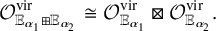 $$ \begin{align*} \mathcal{O}^{\mathrm{vir}}_{\mathbb{E}_{\alpha_1} \boxplus \mathbb{E}_{\alpha_2}} \cong \mathcal{O}^{\mathrm{vir}}_{\mathbb{E}_{\alpha_1}}\boxtimes \mathcal{O}^{\mathrm{vir}}_{\mathbb{E}_{\alpha_2}}. \end{align*} $$
The resulting isomorphisms naturally preserve associativity and commutativity in the sense of Definition 3.5, so that it suffices to show the obstruction theories
 $\mathbb {E}_\alpha $
make a
$\mathbb {E}_\alpha $
make a
 $\boxplus $
-factorizable system. More specifically, we want isomorphisms
$\boxplus $
-factorizable system. More specifically, we want isomorphisms
 $$ \begin{align} \left.{\left(\mathbb{E}_{\alpha_1} \boxplus \mathbb{E}_{\alpha_2}\right)}\right\vert_{U_{\alpha_1 \alpha_2}} \xrightarrow{\sim} \left.{\mathbb{E}_{\alpha_1+\alpha_2}}\right\vert_{U_{\alpha_1 \alpha_2}} \end{align} $$
which are associative and commutative as in Definition 3.5.
Take
 $\alpha _1+\alpha _2=\alpha $
in I and consider the universal family
$\alpha _1+\alpha _2=\alpha $
in I and consider the universal family
 $\mathcal {Z}$
of
$\mathcal {Z}$
of
 $\mathrm {Hilb}^{\alpha }(\mathcal {X})$
, pulled back to
$\mathrm {Hilb}^{\alpha }(\mathcal {X})$
, pulled back to
 $U_{\alpha _1 \alpha _2}\times \mathcal {X}$
. We denote this by
$U_{\alpha _1 \alpha _2}\times \mathcal {X}$
. We denote this by
 $\widetilde {\mathcal {Z}}$
. Over
$\widetilde {\mathcal {Z}}$
. Over
 $U_{\alpha _1 \alpha _2}\times \mathcal {X}$
this splits as
$U_{\alpha _1 \alpha _2}\times \mathcal {X}$
this splits as
 $\widetilde {\mathcal {Z}} = \widetilde {\mathcal {Z}}_1 \sqcup \widetilde {\mathcal {Z}}_2$
, where
$\widetilde {\mathcal {Z}} = \widetilde {\mathcal {Z}}_1 \sqcup \widetilde {\mathcal {Z}}_2$
, where
 $\widetilde {\mathcal {Z}}_i$
are disjoint families of substacks of
$\widetilde {\mathcal {Z}}_i$
are disjoint families of substacks of
 $\mathcal {X}$
of class
$\mathcal {X}$
of class
 $\alpha _i$
. Consider the following commutative diagram.
$\alpha _i$
. Consider the following commutative diagram.

The composition
is just the universal family
 $\mathcal {Z}_i$
restricted to the image of
$\mathcal {Z}_i$
restricted to the image of
 $U_{\alpha _1 \alpha _2}$
in
$U_{\alpha _1 \alpha _2}$
in
 $\mathrm {Hilb}^{\alpha _i}(\mathcal {X})$
. Using this, we obtain a natural isomorphism
$\mathrm {Hilb}^{\alpha _i}(\mathcal {X})$
. Using this, we obtain a natural isomorphism
 $$ \begin{align} j^*p_i^* \mathbb{E}_{\alpha_i} \cong Rp_{U *} R\mathcal{H} om\left(\mathcal{I}_{\tilde{\mathcal{Z}}_i},\mathcal{I}_{\tilde{\mathcal{Z}}_i}\right)_0[2], \end{align} $$
where
 $p_U$
is the projection of
$p_U$
is the projection of
 $U_{\alpha _1 \alpha _2}\times \mathcal {X}$
onto the first factor. We also have a natural isomorphism
$U_{\alpha _1 \alpha _2}\times \mathcal {X}$
onto the first factor. We also have a natural isomorphism
 $$ \begin{align} j^{\prime*} \mathbb{E}_{\alpha_1+\alpha_2} \cong Rp_{U *} R\mathcal{H} om\left(\mathcal{I}_{\tilde{\mathcal{Z}}},\mathcal{I}_{\tilde{\mathcal{Z}}}\right)_0[2]. \end{align} $$
Using disjointness of
 $\widetilde {\mathcal {Z}}_1$
and
$\widetilde {\mathcal {Z}}_1$
and
 $\widetilde {\mathcal {Z}}_2$
, we get a canonical natural isomorphism
$\widetilde {\mathcal {Z}}_2$
, we get a canonical natural isomorphism
 $$ \begin{align*} R\mathcal{H} om\left(\mathcal{I}_{\tilde{\mathcal{Z}}},\mathcal{I}_{\tilde{\mathcal{Z}}}\right)_0 \cong R\mathcal{H} om\left(\mathcal{I}_{\tilde{\mathcal{Z}}_1},\mathcal{I}_{\tilde{\mathcal{Z}}_1}\right)_0\oplus R\mathcal{H} om\left(\mathcal{I}_{\tilde{\mathcal{Z}}_2},\mathcal{I}_{\tilde{\mathcal{Z}}_2}\right)_0, \end{align*} $$
which yields the desired isomorphisms (30) by combining with (32) and (33). Note here, that this isomorphism couldn’t exist without taking the traceless part. Using similar decompositions of the universal family, the required commutativity and associativity properties for these isomorphisms can be shown analogously.
4.1.2 Twisted virtual structure sheaves
Now we see that the twisted virtual structure sheaves of Definition 2.9 make a factorizable system. In contrast to the untwisted virtual structure sheaf, we have to pass to the coarse space X to prove factorizability of the twist.
Proposition 4.2. Let
 $\mathcal {X}$
be a smooth quasi-projective three-dimensional Calabi–Yau orbifold with coarse space X. Consider the factorization index set
$\mathcal {X}$
be a smooth quasi-projective three-dimensional Calabi–Yau orbifold with coarse space X. Consider the factorization index set
 $I\subset \mathrm {N}_0(\mathcal {X})$
of Lemma 3.3. Then
$I\subset \mathrm {N}_0(\mathcal {X})$
of Lemma 3.3. Then
 $$ \begin{align*} \left\{\widehat{\mathcal{O}}^{\mathrm{vir}}_{\mathrm{Hilb}^\alpha(\mathcal{X})}\right\}_{\alpha\in I} \end{align*} $$
is a factorizable system in the sense of Definition 3.5 and Example 3.8.
Proof. Factorization properties are stable under tensor products, and the desired property for
 $\mathcal {O}^{\mathrm {vir}}_{\mathrm {Hilb}^\alpha (\mathcal {X})}$
has already been shown in the proof of Proposition 4.1.
$\mathcal {O}^{\mathrm {vir}}_{\mathrm {Hilb}^\alpha (\mathcal {X})}$
has already been shown in the proof of Proposition 4.1.
Take
 $\alpha _1+\alpha _2=\alpha $
in I and consider the diagram (31) with cartesian squares. We want to compare the sheaves
$\alpha _1+\alpha _2=\alpha $
in I and consider the diagram (31) with cartesian squares. We want to compare the sheaves
 $j^*p_i^* p_{\mathcal {Z}_{i} *}(\mathcal {O}_{\mathcal {Z}_{i}})$
with
$j^*p_i^* p_{\mathcal {Z}_{i} *}(\mathcal {O}_{\mathcal {Z}_{i}})$
with
 $j^* p_{\mathcal {Z} *}(\mathcal {O}_{\mathcal {Z}})$
, where
$j^* p_{\mathcal {Z} *}(\mathcal {O}_{\mathcal {Z}})$
, where
 $\mathcal {Z}_{i}$
are the universal families of
$\mathcal {Z}_{i}$
are the universal families of
 $\mathrm {Hilb}^{\alpha _i}(\mathcal {X})$
and
$\mathrm {Hilb}^{\alpha _i}(\mathcal {X})$
and
 $\mathcal {Z}$
is the universal family of
$\mathcal {Z}$
is the universal family of
 $\mathrm {Hilb}^\alpha (\mathcal {X})$
. Repeatedly applying the push-pull formula yields natural isomorphisms
$\mathrm {Hilb}^\alpha (\mathcal {X})$
. Repeatedly applying the push-pull formula yields natural isomorphisms
 $$ \begin{align*} j^*p_i^* p_{\mathcal{Z}_{i} *}\left(\mathcal{O}_{\mathcal{Z}_{i}}\right) &\cong p_{U_{\alpha_1 \alpha_2} *}\left(\mathcal{O}_{\tilde{\mathcal{Z}}_{i}}\right),\\ j^* p_{\mathcal{Z} *}\left(\mathcal{O}_{\mathcal{Z}}\right) &\cong p_{U_{b_1b_2} *}\left(\mathcal{O}_{\tilde{\mathcal{Z}}}\right). \end{align*} $$
As illustrated in the diagram (31),
 $\widetilde {\mathcal {Z}}$
splits into
$\widetilde {\mathcal {Z}}$
splits into
 $\widetilde {\mathcal {Z}}_{1} \sqcup \widetilde {\mathcal {Z}}_{2}$
. This gives us natural isomorphisms
$\widetilde {\mathcal {Z}}_{1} \sqcup \widetilde {\mathcal {Z}}_{2}$
. This gives us natural isomorphisms
 $$ \begin{align*} p_{U_{b_1b_2} *}\left(\mathcal{O}_{\tilde{\mathcal{Z}}}\right) \cong p_{U_{\alpha_1 \alpha_2} *}\left(\mathcal{O}_{\tilde{\mathcal{Z}}_{1}}\right)\oplus p_{U_{\alpha_1 \alpha_2} *}\left(\mathcal{O}_{\tilde{\mathcal{Z}}_{2}}\right). \end{align*} $$
Because this natural isomorphism is essentially just the splitting of a sheaf into its restriction to connected components of its support, these isomorphisms satisfy the associativity and commutativity assumptions of Definition 3.5 with
 $\boxplus $
. Multiplying by the constant factor
$\boxplus $
. Multiplying by the constant factor
 $\kappa ^{\frac {1}{2}}$
in the equivariant case is compatible with these isomorphisms. Taking determinants preserves these isomorphisms, but the commutativity diagram (11) only commutes up to the sign
$\kappa ^{\frac {1}{2}}$
in the equivariant case is compatible with these isomorphisms. Taking determinants preserves these isomorphisms, but the commutativity diagram (11) only commutes up to the sign
 $(-1)^{\operatorname {\mathrm {rk}} \left(p_{\mathcal {Z}_{1} *}(\mathcal {O}_{\mathcal {Z}_{1}})\right)\operatorname {\mathrm {rk}} \left(p_{\mathcal {Z}_{2} *}(\mathcal {O}_{\mathcal {Z}_{2}})\right)}$
, which by Lemma 2.11 is exactly
$(-1)^{\operatorname {\mathrm {rk}} \left(p_{\mathcal {Z}_{1} *}(\mathcal {O}_{\mathcal {Z}_{1}})\right)\operatorname {\mathrm {rk}} \left(p_{\mathcal {Z}_{2} *}(\mathcal {O}_{\mathcal {Z}_{2}})\right)}$
, which by Lemma 2.11 is exactly
 $(-1)^{b(\alpha _1)b(\alpha _2)}$
. The degree shift of
$(-1)^{b(\alpha _1)b(\alpha _2)}$
. The degree shift of
 $b(\alpha _i)$
of our 2-periodic complexes in Definition 2.9 introduces an additional sign
$b(\alpha _i)$
of our 2-periodic complexes in Definition 2.9 introduces an additional sign
 $(-1)^{b(\alpha _1)b(\alpha _2)}$
in the commutativity of the diagram (11), which exactly cancels the previous sign, and hence makes the twist factorizable.
$(-1)^{b(\alpha _1)b(\alpha _2)}$
in the commutativity of the diagram (11), which exactly cancels the previous sign, and hence makes the twist factorizable.
Remark 4.3. The strategy in the above proof to first show
 $\boxplus $
-factorizability and then taking determinants works more generally and is implicitly already used in [Reference Okounkov31, 5.3.10]. The shifts must be introduced, because taking determinants makes the commutativity diagram only commute up to sign, which can be fixed using these shifts.
$\boxplus $
-factorizability and then taking determinants works more generally and is implicitly already used in [Reference Okounkov31, 5.3.10]. The shifts must be introduced, because taking determinants makes the commutativity diagram only commute up to sign, which can be fixed using these shifts.
Remark 4.4. The shift, which is required to make the diagrams commute, coincides with signs in the literature. For example, in [Reference Cao, Kool and Monavari11, Cor. 6.2], the same sign
 $(-1)^{n_0}$
is introduced as a sign of the formal variable
$(-1)^{n_0}$
is introduced as a sign of the formal variable
 $q_0$
instead of being part of the twisted virtual structure sheaf as in our Definition 2.9. The above lemma shows that this sign is exactly the sign making the system of twisted virtual structure sheaves factorizable.
$q_0$
instead of being part of the twisted virtual structure sheaf as in our Definition 2.9. The above lemma shows that this sign is exactly the sign making the system of twisted virtual structure sheaves factorizable.
Lemma 4.5. Let
 $\mathcal {X}$
be a smooth three-dimensional orbifold, and let U be its nonstacky locus. Consider the factorization index set
$\mathcal {X}$
be a smooth three-dimensional orbifold, and let U be its nonstacky locus. Consider the factorization index set
 $I\subset \mathrm {N}_0(\mathcal {X})$
of Lemma 3.3. By Proposition 4.2, Lemma 3.11 and Example 3.12, we have the factorizable system
$I\subset \mathrm {N}_0(\mathcal {X})$
of Lemma 3.3. By Proposition 4.2, Lemma 3.11 and Example 3.12, we have the factorizable system
It satisfies that for any
 $\alpha \in I\setminus \Delta _I$
,
$\alpha \in I\setminus \Delta _I$
,
 $\mathcal {F}_{\alpha }$
vanishes on
$\mathcal {F}_{\alpha }$
vanishes on
 $\mathrm {Sym}^{b(\alpha )}(U)$
.
$\mathrm {Sym}^{b(\alpha )}(U)$
.
Proof. Set
 $\eta _\alpha = \xi _\alpha \circ \mathrm {HC}_\alpha $
. We have the cartesian diagram
$\eta _\alpha = \xi _\alpha \circ \mathrm {HC}_\alpha $
. We have the cartesian diagram

This gives us
 $$ \begin{align*} \left.{\mathcal{F}_\alpha}\right\vert_{\mathrm{Sym}^{b(\alpha)}(U)} \cong \left(\eta_\alpha^U\right)_*\left(\left.{\widehat{\mathcal{O}}^{\mathrm{vir}}_{\mathrm{Hilb}^\alpha(\mathcal{X})}}\right\vert_{\mathrm{Hilb}^\alpha(U)}\right), \end{align*} $$
but any substack of U has class in
 $\Delta _I$
by definition. So, for a class
$\Delta _I$
by definition. So, for a class
 $\alpha \in I\setminus \Delta _I$
,
$\alpha \in I\setminus \Delta _I$
,
 $\mathrm {Hilb}^\alpha (U)$
is empty, proving
$\mathrm {Hilb}^\alpha (U)$
is empty, proving
 $\left.{\mathcal {F}_\alpha }\right\vert _{\mathrm {Sym}^{b(\alpha )}(U)}$
vanishes.
$\left.{\mathcal {F}_\alpha }\right\vert _{\mathrm {Sym}^{b(\alpha )}(U)}$
vanishes.
4.2 Orbifold generating series
4.2.1 Orbifold generating series
For a given smooth quasi-projective Calabi–Yau orbifold
 $\mathcal {X}$
of dimension three, we apply the factorization theorem to simplify its generating series of (equivariant) Donaldson–Thomas invariants. Let I be the factorization index set of Lemma 3.3. As
$\mathcal {X}$
of dimension three, we apply the factorization theorem to simplify its generating series of (equivariant) Donaldson–Thomas invariants. Let I be the factorization index set of Lemma 3.3. As
 $\mathrm {Hilb}^{\alpha }(\mathcal {X})$
is empty for
$\mathrm {Hilb}^{\alpha }(\mathcal {X})$
is empty for
 $\alpha \notin I$
by definition, it suffices to sum over
$\alpha \notin I$
by definition, it suffices to sum over
 $\alpha \in I$
in the generating series
$\alpha \in I$
in the generating series
 $\mathsf {Z}(\mathcal {X})$
. As seen above, the pushforwards of the twisted virtual structure sheaves
$\mathsf {Z}(\mathcal {X})$
. As seen above, the pushforwards of the twisted virtual structure sheaves
 $\widehat {\mathcal {O}}^{vir}$
on
$\widehat {\mathcal {O}}^{vir}$
on
 $\mathrm {Hilb}^\alpha (\mathcal {X})$
to
$\mathrm {Hilb}^\alpha (\mathcal {X})$
to
 $\mathrm {Sym}^{b(\alpha )}(X)$
yield a factorizable system of sheaves.
$\mathrm {Sym}^{b(\alpha )}(X)$
yield a factorizable system of sheaves.
We assume from now on that I is closed under addition. Note that the factorization index set of Lemma 3.3 is closed under addition for orbifolds of the form
 $\mathcal {X}=\mathcal {X}'\times \mathbb {C}$
, which we are mainly interested in. By Theorem 3.22, there are classes
$\mathcal {X}=\mathcal {X}'\times \mathbb {C}$
, which we are mainly interested in. By Theorem 3.22, there are classes
 $$ \begin{align*} [\mathcal{G}_\alpha]\in K(X)\text{ for }\alpha\in \Delta_I,\quad [\mathcal{G}_\alpha]\in K(S)\text{ for }\alpha\notin \Delta_I, \end{align*} $$
such that the generating series equals
 $$ \begin{align*} \mathsf{Z}(\mathcal{X}) &= 1+\sum_{\alpha\in I} q^{\alpha} \chi\left(\mathrm{Hilb}^{\alpha}(\mathcal{X}),\widehat{\mathcal{O}}^{\mathrm{vir}}_{\mathrm{Hilb}^{\alpha}(\mathcal{X})}\right)\\ &= \mathrm{PExp}\,\left(\sum_{\alpha\in \Delta_I}q^{\alpha} \chi\left(X,\mathcal{G}_{\alpha}\right) + \sum_{\alpha\in I\setminus\Delta_I}q^{\alpha} \chi\left(S,\mathcal{G}_{\alpha}\right)\right). \end{align*} $$
4.2.2 Crepant resolutions and compatible factorization
Recall that we are working with a fixed coarse moduli space
 $\pi :\mathcal {X}\to X$
. Let
$\pi :\mathcal {X}\to X$
. Let
 $\nu :Y\to X$
be a crepant resolution. Let U be the nonstacky locus and let S be its complement in the coarse moduli space. Note that U also openly embeds into Y. Let E be its complement in Y. Take a fixed point p in U to define
$\nu :Y\to X$
be a crepant resolution. Let U be the nonstacky locus and let S be its complement in the coarse moduli space. Note that U also openly embeds into Y. Let E be its complement in Y. Take a fixed point p in U to define
 $\Delta _I=\mathbb {N} [\mathcal {O}_p]$
. We can compute the equivariant K-theoretic generating function for
$\Delta _I=\mathbb {N} [\mathcal {O}_p]$
. We can compute the equivariant K-theoretic generating function for
 $\mathrm {Hilb}^n(Y)$
using Nekrasov’s formula [Reference Okounkov31, Theorem 3.3.6]. We have the following identification
$\mathrm {Hilb}^n(Y)$
using Nekrasov’s formula [Reference Okounkov31, Theorem 3.3.6]. We have the following identification
 $$ \begin{align*} \mathrm{Hilb}^n(Y) \hookleftarrow \mathrm{Hilb}^n(U) \xrightarrow{\sim} \mathrm{Hilb}^{n[\mathcal{O}_p]}(U) \hookrightarrow \mathrm{Hilb}^{n[\mathcal{O}_p]}(\mathcal{X}). \end{align*} $$
The obstruction theories agree under this isomorphism, since the deformation theory of sheaves restricts naturally to open substacks. This gives us the required isomorphisms for compatible factorization, so the twisted virtual structure sheaves are compatibly factorizable along the embeddings
 $U\hookrightarrow Y$
and
$U\hookrightarrow Y$
and
 $U\hookrightarrow \mathcal {X}$
respectively. Pushforward along the open embeddings embeds the factorization index semigroup
$U\hookrightarrow \mathcal {X}$
respectively. Pushforward along the open embeddings embeds the factorization index semigroup
 $I_U=\mathbb {N}$
into
$I_U=\mathbb {N}$
into
 $I_Y=\mathbb {N}$
by the identity and into
$I_Y=\mathbb {N}$
by the identity and into
 $I_{\mathcal {X}}$
by
$I_{\mathcal {X}}$
by
 $n\mapsto n[\mathcal {O}_p]$
.
$n\mapsto n[\mathcal {O}_p]$
.
Again, we assume that
 $I_{\mathcal {X}}$
is closed under addition. Applying Theorem 3.57, we get
$I_{\mathcal {X}}$
is closed under addition. Applying Theorem 3.57, we get
 $$ \begin{align*} \left[\left.{\mathcal{G}_{n[\mathcal{O}_p]}^{\mathcal{X}}}\right\vert_{U}\right] = \left[\left.{\mathcal{G}_{n}^Y}\right\vert_{U}\right]. \end{align*} $$
Hence, the class
 $\left[\mathcal {G}_{n[\mathcal {O}_p]}^{\mathcal {X}}\right] - \left[\nu _*\mathcal {G}_{n}^Y\right]$
is supported on S. By dévissage [Reference Weibel38, Appl. 6.4.2], it must be the pushforward of some class
$\left[\mathcal {G}_{n[\mathcal {O}_p]}^{\mathcal {X}}\right] - \left[\nu _*\mathcal {G}_{n}^Y\right]$
is supported on S. By dévissage [Reference Weibel38, Appl. 6.4.2], it must be the pushforward of some class
 $\left[\mathcal {G}_{n[\mathcal {O}_p]}^S\right]\in K(S)$
. By invariance of
$\left[\mathcal {G}_{n[\mathcal {O}_p]}^S\right]\in K(S)$
. By invariance of
 $\chi $
under pushforwards, we obtain
$\chi $
under pushforwards, we obtain
 $$ \begin{align*} \chi\left(X,\mathcal{G}_{n[\mathcal{O}_p]}^{\mathcal{X}}\right) = \chi\left(Y,\mathcal{G}_{n}^Y\right) + \chi\left(S, \mathcal{G}_{n[\mathcal{O}_p]}^S\right). \end{align*} $$
Putting all these parts together, we obtain the following form.
Proposition 4.6. Let
 $\pi :\mathcal {X}\to X$
be the coarse moduli space, and let
$\pi :\mathcal {X}\to X$
be the coarse moduli space, and let
 $\nu :Y\to X$
be a crepant resolution. Let U be the nonstacky locus and let S be its complement in the coarse moduli space. Assume that the factorization index set
$\nu :Y\to X$
be a crepant resolution. Let U be the nonstacky locus and let S be its complement in the coarse moduli space. Assume that the factorization index set
 $I_{\mathcal {X}}$
of Lemma 3.3 is closed under addition. We have the equation
$I_{\mathcal {X}}$
of Lemma 3.3 is closed under addition. We have the equation
 $$ \begin{align*} \begin{aligned} Z(\mathcal{X}) =&\ \mathrm{PExp}\,\left(\sum_{n>0}q^{n[\mathcal{O}_p]} \left(\chi\left(Y,\mathcal{G}_{n}^Y\right)+\chi\left(S,\mathcal{G}^S_{n[\mathcal{O}_p]}\right)\right) + \sum_{\alpha\in I\setminus \Delta_I} q^{\alpha} \chi\left(S,\mathcal{G}_{\alpha}^{\mathcal{X}}\right)\right)\\ =&\ Z(Y,q^{[\mathcal{O}_p]}) \cdot \mathrm{PExp}\,\left(\sum_{n>0}q^{n[\mathcal{O}_p]} \chi\left(S,\mathcal{G}^S_{n[\mathcal{O}_p]}\right) + \sum_{\alpha\in I\setminus \Delta_I} q^{\alpha} \chi\left(S,\mathcal{G}_{\alpha}^{\mathcal{X}}\right)\right) \end{aligned} \end{align*} $$
where
 $Z(Y,q)$
is the equivariant K-theoretic generating function for the Hilbert schemes of points on Y.
$Z(Y,q)$
is the equivariant K-theoretic generating function for the Hilbert schemes of points on Y.
5 Rigidity
5.1 Orbifold computation
Now we specialize to our specific situation with
 $\mu _r$
acting on
$\mu _r$
acting on
 $\mathbb {C}^3$
with weight
$\mathbb {C}^3$
with weight
 $(1,r-1,0)$
. Let
$(1,r-1,0)$
. Let
 $\mathsf {T}=(\mathbb {C}^*)^3$
act by
$\mathsf {T}=(\mathbb {C}^*)^3$
act by
 $(t_1,t_2,t_3)$
on
$(t_1,t_2,t_3)$
on
 $\mathbb {C}^3$
. In this section, we will prove the following theorem.
$\mathbb {C}^3$
. In this section, we will prove the following theorem.
Theorem 5.1. The
 $\mathsf {T}$
-equivariant K-theoretic degree
$\mathsf {T}$
-equivariant K-theoretic degree
 $0$
DT generating series for
$0$
DT generating series for
 $[\mathbb {C}^3/\mu _r]$
, with
$[\mathbb {C}^3/\mu _r]$
, with
 $\mu _r$
acting on
$\mu _r$
acting on
 $\mathbb {C}^3$
with weight
$\mathbb {C}^3$
with weight
 $(1,r-1,0)$
, is
$(1,r-1,0)$
, is
 $$ \begin{align*} \mathsf{Z}\left([\mathbb{C}^3/\mu_r],q_0,\dots,q_{r-1}\right) = \mathrm{PExp}\,\left(\mathsf{F}_r(q)+\mathsf{F}_r^{\mathrm{col}}(q_0,\dots,q_{r-1})\right), \end{align*} $$
where

where
 $q=q_0\cdots q_{r-1}$
,
$q=q_0\cdots q_{r-1}$
,
 $q_{[i,j]}=q_i\cdots q_j$
,
$q_{[i,j]}=q_i\cdots q_j$
,
 $[w]=w^{1/2}-w^{-1/2}$
, and
$[w]=w^{1/2}-w^{-1/2}$
, and
 $\mathrm {PExp}\left(\cdot \right)$
denotes the plethystic exponential. Note that the factorization index set I of Lemma 3.3 is closed under addition in this case.
$\mathrm {PExp}\left(\cdot \right)$
denotes the plethystic exponential. Note that the factorization index set I of Lemma 3.3 is closed under addition in this case.
The proof occupies the remainder of the section. As
 $\mu _r$
acts trivially on the third coordinate, the crepant resolution of the coarse moduli space of
$\mu _r$
acts trivially on the third coordinate, the crepant resolution of the coarse moduli space of
 $[\mathbb {C}^3/\mu _r]$
is given by
$[\mathbb {C}^3/\mu _r]$
is given by
 $Y=\mathcal {A}_{r-1}\times \mathbb {C}$
, where
$Y=\mathcal {A}_{r-1}\times \mathbb {C}$
, where
 $\mathcal {A}_{r-1}$
is the minimal resolution of
$\mathcal {A}_{r-1}$
is the minimal resolution of
 $[\mathbb {C}^2/\mu _r]$
. A toric description of
$[\mathbb {C}^2/\mu _r]$
. A toric description of
 $\mathcal {A}_{r-1}$
can be found in [Reference Cox, Little and Schenck14, §10.1]. From this description we obtain r charts of Y isomorphic to
$\mathcal {A}_{r-1}$
can be found in [Reference Cox, Little and Schenck14, §10.1]. From this description we obtain r charts of Y isomorphic to
 $\mathbb {C}^3$
with weights
$\mathbb {C}^3$
with weights
 $\left(t_1^{r-k}t_2^{-k},t_1^{-r+k+1}t_2^{k+1},t_3\right)$
, where
$\left(t_1^{r-k}t_2^{-k},t_1^{-r+k+1}t_2^{k+1},t_3\right)$
, where
 $0\leq k\leq r-1$
. Localization together with Nekrasov’s formula [Reference Okounkov31, Theorem 3.3.6] then lets us compute
$0\leq k\leq r-1$
. Localization together with Nekrasov’s formula [Reference Okounkov31, Theorem 3.3.6] then lets us compute
 $$ \begin{align*} \mathsf{Z}(Y,q) = \mathrm{PExp}\,\left(\mathsf{F}_r(q)\right). \end{align*} $$
By computing the Euler characteristics in Proposition 4.6 via localization on S, and by inserting the above formula for
 $\mathsf {Z}(Y,q)$
, we obtain the following.
$\mathsf {Z}(Y,q)$
, we obtain the following.
Proposition 5.2. For
 $\mu _r$
acting on
$\mu _r$
acting on
 $\mathbb {C}^3$
with weight
$\mathbb {C}^3$
with weight
 $(1,r-1,0)$
, we have
$(1,r-1,0)$
, we have
 $$ \begin{align} \mathsf{Z}\left([\mathbb{C}^3/\mu_r],\mathbf{q}\right) = \mathrm{PExp}\,\left(\mathsf{F}_r(q)\right)\cdot \mathrm{PExp}\,\left(\frac{[t_1t_2]}{[t_3]}\sum_{\mathbf{n}\in I} \mathbf{q}^{\mathbf{n}} h_{\mathbf{n}}\right), \end{align} $$
with
 $h_{\mathbf {n}}$
in
$h_{\mathbf {n}}$
in
 $\mathbb {Z}[t_1^{\pm 1/2},t_2^{\pm 1/2},t_3^{\pm 1/2}]$
.
$\mathbb {Z}[t_1^{\pm 1/2},t_2^{\pm 1/2},t_3^{\pm 1/2}]$
.
Proof. We insert the
 $\mathsf {Z}(Y,q)$
of the crepant resolution computed above into Proposition 4.6. Then we note that S is the coarse moduli space of
$\mathsf {Z}(Y,q)$
of the crepant resolution computed above into Proposition 4.6. Then we note that S is the coarse moduli space of
 $[\mathrm {pt}/\mu _r]\times \mathbb {C}$
, which is just
$[\mathrm {pt}/\mu _r]\times \mathbb {C}$
, which is just
 $\mathbb {C}$
, with
$\mathbb {C}$
, with
 $\mathsf {T}$
acting just by
$\mathsf {T}$
acting just by
 $t_3$
. So, localization on S gives us
$t_3$
. So, localization on S gives us
 $$ \begin{align*} \mathsf{Z}\left([\mathbb{C}^3/\mu_r],\mathbf{q}\right) = \mathrm{PExp}\,\left(\mathsf{F}_r(q)\right)\cdot \mathrm{PExp}\,\left(\frac{1}{1-t_3^{-1}}\sum_{\mathbf{n}\in I} \mathbf{q}^{\mathbf{n}} \tilde{h}_{\mathbf{n}}\right), \end{align*} $$
for some
 $\tilde {h}_{\mathbf {n}}$
in
$\tilde {h}_{\mathbf {n}}$
in
 $\mathbb {Z}[t_1^{\pm 1/2},t_2^{\pm 1/2},t_3^{\pm 1/2}]$
. Note here that localization on
$\mathbb {Z}[t_1^{\pm 1/2},t_2^{\pm 1/2},t_3^{\pm 1/2}]$
. Note here that localization on
 $S=\mathbb {C}$
always yields a rational function made up of
$S=\mathbb {C}$
always yields a rational function made up of
 $\frac {1}{1-t_3^{-1}}$
multiplied by a Laurent polynomial in the equivariant parameters.
$\frac {1}{1-t_3^{-1}}$
multiplied by a Laurent polynomial in the equivariant parameters.
To show the proposition, we claim that all
 $\tilde {h}_{(n_0,n_1)}$
are divisible by
$\tilde {h}_{(n_0,n_1)}$
are divisible by
 $t_1t_2-1$
. Then since
$t_1t_2-1$
. Then since
 $\kappa ^{1/2}\frac {[t_1t_2]}{[t_3]}=\frac {t_1t_2-1}{1-t_3^{-1}}$
, we can take
$\kappa ^{1/2}\frac {[t_1t_2]}{[t_3]}=\frac {t_1t_2-1}{1-t_3^{-1}}$
, we can take ![]() . Since the
. Since the
 $\tilde {h}_{\mathbf {n}}$
are Laurent in the equivariant parameters, so are the
$\tilde {h}_{\mathbf {n}}$
are Laurent in the equivariant parameters, so are the
 $h_{\mathbf {n}}$
.
$h_{\mathbf {n}}$
.
By invertibility of the plethystic exponential, it suffices to prove that any localization weight in
 $\mathsf {Z}\left([\mathbb {C}^3/\mu _r],q_0,q_1\right)$
is divisible by
$\mathsf {Z}\left([\mathbb {C}^3/\mu _r],q_0,q_1\right)$
is divisible by
 $t_1t_2-1$
. By the localization weights
$t_1t_2-1$
. By the localization weights
 $\hat {a}(\pi )$
, which we computed in Section 2.4.4, we need to check that
$\hat {a}(\pi )$
, which we computed in Section 2.4.4, we need to check that
 $t_1t_2$
has negative coefficient in the class of the virtual tangent space at
$t_1t_2$
has negative coefficient in the class of the virtual tangent space at
 $\pi $
. By the natural identification (5), the virtual tangent space at
$\pi $
. By the natural identification (5), the virtual tangent space at
 $\pi $
is exactly the
$\pi $
is exactly the
 $\mu _r$
-fixed part of the virtual tangent space of
$\mu _r$
-fixed part of the virtual tangent space of
 $\mathrm {Hilb}(\mathbb {C}^3)$
at the fixed point corresponding to the underlying plane partition of
$\mathrm {Hilb}(\mathbb {C}^3)$
at the fixed point corresponding to the underlying plane partition of
 $\pi $
. Now [Reference Maulik, Nekrasov, Okounkov and Pandharipande26, Lemma 5] shows that the virtual tangent space of
$\pi $
. Now [Reference Maulik, Nekrasov, Okounkov and Pandharipande26, Lemma 5] shows that the virtual tangent space of
 $\mathrm {Hilb}(\mathbb {C}^3)$
at each fixed point has negative coefficient of
$\mathrm {Hilb}(\mathbb {C}^3)$
at each fixed point has negative coefficient of
 $t_1t_2$
. Taking the
$t_1t_2$
. Taking the
 $\mu _r$
-invariant part retains this negative coefficient.
$\mu _r$
-invariant part retains this negative coefficient.
Applying Okounkov’s rigidity principle, we can refine this proposition as follows.
Lemma 5.3. The functions
 $h_{\mathbf {n}}$
in Proposition 5.2 are in
$h_{\mathbf {n}}$
in Proposition 5.2 are in
 $\mathbb {Z}[\kappa ^{\pm 1}]$
, that is, they are only dependent on
$\mathbb {Z}[\kappa ^{\pm 1}]$
, that is, they are only dependent on
 $\kappa $
, not
$\kappa $
, not
 $t_1,t_2,t_3$
.
$t_1,t_2,t_3$
.
Proof. We follow the proof of [Reference Okounkov31, Prop. 3.5.11]. For any
 $\mathsf {T}$
-weight w, the fraction
$\mathsf {T}$
-weight w, the fraction
 $$ \begin{align*} \frac{[\kappa/w]}{[w]} \end{align*} $$
remains bounded for any limit
 $t_i^{\pm 1}\to \infty $
that keeps
$t_i^{\pm 1}\to \infty $
that keeps
 $\kappa $
fixed. That means all terms of the first factor in (34) as well as the local contributions
$\kappa $
fixed. That means all terms of the first factor in (34) as well as the local contributions
 $\hat {a}(\pi )$
to
$\hat {a}(\pi )$
to
 $\mathsf {Z}([\mathbb {C}^3/\mu _r])$
from Section 2.4.4 and
$\mathsf {Z}([\mathbb {C}^3/\mu _r])$
from Section 2.4.4 and
 $\frac {[t_1t_2]}{[t_3]}$
in the second factor of (34) remain bounded under any such limit.
$\frac {[t_1t_2]}{[t_3]}$
in the second factor of (34) remain bounded under any such limit.
If we can prove that all
 $h_{\mathbf {n}}$
from Proposition 5.2 remain bounded under any limit
$h_{\mathbf {n}}$
from Proposition 5.2 remain bounded under any limit
 $t_i^{\pm 1}\to \infty $
that keeps
$t_i^{\pm 1}\to \infty $
that keeps
 $\kappa $
fixed, then as Laurent polynomials, they only depend on
$\kappa $
fixed, then as Laurent polynomials, they only depend on
 $\kappa $
and not on the
$\kappa $
and not on the
 $t_i$
. To show this, we work by induction in I. For any I-indecomposable element
$t_i$
. To show this, we work by induction in I. For any I-indecomposable element
 $\mathbf {n}$
in I, the coefficient of
$\mathbf {n}$
in I, the coefficient of
 $\mathbf {q}^{\mathbf {n}}$
in the right-hand side of (34) is just
$\mathbf {q}^{\mathbf {n}}$
in the right-hand side of (34) is just
 $$ \begin{align*} \frac{[t_1t_2]}{[t_3]}h_{\mathbf{n}}, \end{align*} $$
plus a term coming from the first factor of the right-hand side of (34) if
 $\mathbf {n}\in \Delta _I$
. As the other terms of the equation resulting from taking
$\mathbf {n}\in \Delta _I$
. As the other terms of the equation resulting from taking
 $\mathbf {q}^{\mathbf {n}}$
-coefficients in (34), as well as
$\mathbf {q}^{\mathbf {n}}$
-coefficients in (34), as well as
 $\frac {[t_1t_2]}{[t_3]}$
, are bounded under limits
$\frac {[t_1t_2]}{[t_3]}$
, are bounded under limits
 $t_i^{\pm 1}\to \infty $
keeping
$t_i^{\pm 1}\to \infty $
keeping
 $\kappa $
fixed, so is
$\kappa $
fixed, so is
 $h_{\mathbf {n}}$
. In particular, we have shown this property for
$h_{\mathbf {n}}$
. In particular, we have shown this property for
 $\mathbf {n}$
with
$\mathbf {n}$
with
 $\left| \mathbf {n} \right|=1$
.
$\left| \mathbf {n} \right|=1$
.
Assume the desired limit property is shown for all I-indecomposable
 $\mathbf {n}$
and all
$\mathbf {n}$
and all
 $\mathbf {n}$
with
$\mathbf {n}$
with
 $\left| \mathbf {n} \right|<N$
. If
$\left| \mathbf {n} \right|<N$
. If
 $\mathbf {n}$
in I is not I-indecomposable with
$\mathbf {n}$
in I is not I-indecomposable with
 $\left| \mathbf {n} \right|=N$
, the
$\left| \mathbf {n} \right|=N$
, the
 $\mathbf {q}^{\mathbf {n}}$
-coefficient in the right-hand side of (34) consists of one term
$\mathbf {q}^{\mathbf {n}}$
-coefficient in the right-hand side of (34) consists of one term
 $$ \begin{align*} \frac{[t_1t_2]}{[t_3]}h_{\mathbf{n}}, \end{align*} $$
plus other terms, which are products of
 $\frac {[t_1t_2]}{[t_3]}$
,
$\frac {[t_1t_2]}{[t_3]}$
,
 $h_{\mathbf {n}}$
with
$h_{\mathbf {n}}$
with
 $\left| \mathbf {n} \right|<N$
, and terms from the first factor of (34). All of these other terms,
$\left| \mathbf {n} \right|<N$
, and terms from the first factor of (34). All of these other terms,
 $\mathbf {q}^{\mathbf {n}}$
-coefficient in the left-hand side of (34), as well as
$\mathbf {q}^{\mathbf {n}}$
-coefficient in the left-hand side of (34), as well as
 $\frac {[t_1t_2]}{[t_3]}$
remain bounded under limits
$\frac {[t_1t_2]}{[t_3]}$
remain bounded under limits
 $t_i^{\pm 1}\to \infty $
keeping
$t_i^{\pm 1}\to \infty $
keeping
 $\kappa $
fixed. So, the same holds for
$\kappa $
fixed. So, the same holds for
 $h_{\mathbf {n}}$
.
$h_{\mathbf {n}}$
.
5.2 Equivariant limit computation
We want to compute the equivariant K-theoretic Donaldson–Thomas partition function from the result of Proposition 5.2. To determine the functions
 $h_{\mathbf {n}}$
in Proposition 5.2, using Lemma 5.3, it suffices to compute a limit in the
$h_{\mathbf {n}}$
in Proposition 5.2, using Lemma 5.3, it suffices to compute a limit in the
 $\mathsf {T}$
-parameters which fixes
$\mathsf {T}$
-parameters which fixes
 $\kappa $
. We modify the computation of colored plane partition counts in [Reference Young39] to compute this limit.
$\kappa $
. We modify the computation of colored plane partition counts in [Reference Young39] to compute this limit.
Following the proof of Nekrasov’s formula in [Reference Okounkov31, 3.5.12], we compute the limit in the equivariant parameters
 $t_1,t_2,t_3$
, which sends
$t_1,t_2,t_3$
, which sends
 $$ \begin{align} t_1,t_3\to 0,\ \lvert t_1 \rvert\ll\lvert t_3\rvert,\ \kappa\ \mathrm{fixed}. \end{align} $$
We denote the limit of the generating series under this limit of equivariant parameters by
 $$ \begin{align*} \overrightarrow{\mathsf{Z}}\left([\mathbb{C}^3/\mu_r],\mathbf{q}\right). \end{align*} $$
In order to compute this limit using the argument in [Reference Young39], we need the following analogue of a result from [Reference Okounkov31, 3.5.18].
Proposition 5.4. The contribution of the colored partition
 $\pi $
to the
$\pi $
to the
 $\mathsf {T}$
-equivariant K-theoretic count in the above specified limit of its parameters is
$\mathsf {T}$
-equivariant K-theoretic count in the above specified limit of its parameters is
 $\left(-\kappa ^{1/2}\right)^{\mathsf {index}(\pi )}$
, where
$\left(-\kappa ^{1/2}\right)^{\mathsf {index}(\pi )}$
, where
 $$ \begin{align*} \mathsf{index}(\pi) = \sum_{\Box=(i_1,i_2,i_3)\in\pi^G}\mathrm{sgn}(i_2-i_1), \end{align*} $$
where we recall that
 $\pi ^G$
denotes the
$\pi ^G$
denotes the
 $0$
-colored boxes of
$0$
-colored boxes of
 $\pi $
.
$\pi $
.
Proof. As computed in Section 2.4.4, the contribution of the colored partition
 $\pi $
to the
$\pi $
to the
 $\mathsf {T}$
-equivariant K-theoretic count is
$\mathsf {T}$
-equivariant K-theoretic count is
 $$ \begin{align*} \hat{a}(\pi) = \prod_{w\in W} \frac{[\kappa/w]}{[w]}, \end{align*} $$
where W is a subset of the
 $\mathsf {T}$
-weights of the virtual tangent space at
$\mathsf {T}$
-weights of the virtual tangent space at
 $\pi $
, such that
$\pi $
, such that
 $\mathbb {T}_{\mathcal {X},\pi }^{\mathrm {vir}} = \sum _{w\in W} \left(w-\frac {\kappa }{w}\right)$
. The limits of
$\mathbb {T}_{\mathcal {X},\pi }^{\mathrm {vir}} = \sum _{w\in W} \left(w-\frac {\kappa }{w}\right)$
. The limits of
 $\frac {[\kappa /w]}{[w]}$
can be computed
$\frac {[\kappa /w]}{[w]}$
can be computed
 $$ \begin{align*} \frac{[\kappa/w]}{[w]} \to \begin{cases} -\kappa^{-1/2}, & w\to\infty,\\ -\kappa^{1/2}, & w\to 0. \end{cases} \end{align*} $$
Hence, the limit of
 $\hat {a}(\pi )$
becomes
$\hat {a}(\pi )$
becomes
 $$ \begin{align*} \hat{a}(\pi) \to (-\kappa^{1/2})^{\mathsf{index}(\pi)}, \end{align*} $$
where we set
Now we want to find the above expression of this index. Note first, that, since
 $\kappa $
is fixed by the limit, the weights w and
$\kappa $
is fixed by the limit, the weights w and
 $\frac {\kappa }{w}$
of the virtual tangent space have opposite limits. To compute this limit, we want to use the index computation in [Reference Nekrasov and Okounkov27, Appendix A]. For a
$\frac {\kappa }{w}$
of the virtual tangent space have opposite limits. To compute this limit, we want to use the index computation in [Reference Nekrasov and Okounkov27, Appendix A]. For a
 $\mathsf {T}$
-representation V, given as a linear combination of weights
$\mathsf {T}$
-representation V, given as a linear combination of weights
 $V=\sum _w c_w w$
with
$V=\sum _w c_w w$
with
 $c_w\in \mathbb {C}$
, their index is defined as
$c_w\in \mathbb {C}$
, their index is defined as

Inserting
 $\mathbb {T}_{\mathcal {X},\pi }^{\mathrm {vir}} = \sum _{w\in W} \left(w-\frac {\kappa }{w}\right)$
, we have
$\mathbb {T}_{\mathcal {X},\pi }^{\mathrm {vir}} = \sum _{w\in W} \left(w-\frac {\kappa }{w}\right)$
, we have
 $$ \begin{align*} \mathsf{index}(\pi) = \mathsf{index}\left(\mathbb{T}_{\mathcal{X},\pi}^{\mathrm{vir}}\right). \end{align*} $$
By (5),
 $\mathbb {T}_{\mathcal {X},\pi }^{\mathrm {vir}} $
is the
$\mathbb {T}_{\mathcal {X},\pi }^{\mathrm {vir}} $
is the
 $\mu _r$
-equivariant part of
$\mu _r$
-equivariant part of
 $\mathbb {T}_{\mathbb {C}^3,\pi }^{\mathrm {vir}}$
and [Reference Nekrasov and Okounkov27, Appendix A] show
$\mathbb {T}_{\mathbb {C}^3,\pi }^{\mathrm {vir}}$
and [Reference Nekrasov and Okounkov27, Appendix A] show
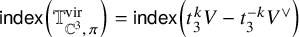 $\mathsf {index}\left(\mathbb {T}_{\mathbb {C}^3,\pi }^{\mathrm {vir}}\right)=\mathsf {index}\left(t_3^kV-t_3^{-k}V^\vee \right)$
for k sufficiently large, but such that still
$\mathsf {index}\left(\mathbb {T}_{\mathbb {C}^3,\pi }^{\mathrm {vir}}\right)=\mathsf {index}\left(t_3^kV-t_3^{-k}V^\vee \right)$
for k sufficiently large, but such that still
 $\left| t_1 \right|\ll \left| t_3 \right|^k$
. Here, V is the character of
$\left| t_1 \right|\ll \left| t_3 \right|^k$
. Here, V is the character of
 $\mathcal {O}_{Z_\pi }$
.
$\mathcal {O}_{Z_\pi }$
.
We want to show a similar identity for the
 $\mu _r$
-invariant parts
$\mu _r$
-invariant parts
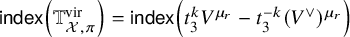 $\mathsf {index}\left(\mathbb {T}_{\mathcal {X},\pi }^{\mathrm {vir}}\right)=\mathsf {index}\left(t_3^kV^{\mu _r}-t_3^{-k}(V^\vee )^{\mu _r}\right)$
. Note that the claim of the proposition follows immediately from such an identity, because
$\mathsf {index}\left(\mathbb {T}_{\mathcal {X},\pi }^{\mathrm {vir}}\right)=\mathsf {index}\left(t_3^kV^{\mu _r}-t_3^{-k}(V^\vee )^{\mu _r}\right)$
. Note that the claim of the proposition follows immediately from such an identity, because
 $$ \begin{align*} V^{\mu_r} = \sum_{\Box=(i_1,i_2,i_3)\in\pi^G} t_1^{-i_1}t_2^{-i_2}t_3^{-i_3}, \end{align*} $$
and
 $$ \begin{align*} t_3^k t_1^{-i_1}t_2^{-i_2}t_3^{-i_3} \to \begin{cases} 0, & , i_2\geq i_1\\ \infty, &, i_2 < i_1, \end{cases} \end{align*} $$
which gives us
 $$ \begin{align*} \mathsf{index}\left(\mathbb{T}_{\mathcal{X},\pi}^{\mathrm{vir}}\right)=\mathsf{index}(t_3^kV^{\mu_r}-t_3^{-k}(V^\vee)^{\mu_r}) = \sum_{\Box=(i_1,i_2,i_3)\in\pi^G}\mathrm{sgn}(i_2-i_1). \end{align*} $$
To prove
 $\mathsf {index}(\mathbb {T}_{\mathcal {X},\pi }^{\mathrm {vir}})=\mathsf {index}(t_3^kV^{\mu _r}-t_3^{-k}(V^\vee )^{\mu _r})$
, we cannot directly use the result of [Reference Nekrasov and Okounkov27, Appendix A], but we will follow their proof. Note first, that since the
$\mathsf {index}(\mathbb {T}_{\mathcal {X},\pi }^{\mathrm {vir}})=\mathsf {index}(t_3^kV^{\mu _r}-t_3^{-k}(V^\vee )^{\mu _r})$
, we cannot directly use the result of [Reference Nekrasov and Okounkov27, Appendix A], but we will follow their proof. Note first, that since the
 $\kappa $
is fixed in the limit, the index is independent of the value of
$\kappa $
is fixed in the limit, the index is independent of the value of
 $\kappa $
, so we may work with the subtorus
$\kappa $
, so we may work with the subtorus
 $\mathsf {A}=\{\kappa =1\}\subset \mathsf {T}$
. In [Reference Nekrasov and Okounkov27, A.1.3], they identify the
$\mathsf {A}=\{\kappa =1\}\subset \mathsf {T}$
. In [Reference Nekrasov and Okounkov27, A.1.3], they identify the
 $\mathsf {A}$
-characters
$\mathsf {A}$
-characters
 $$ \begin{align*} \mathbb{T}_{\mathbb{C}^3,\pi}^{\mathrm{vir}} = (1-t_3)\mathcal{N}_2(Z_\pi) + t_3^kV - t_3^{-k}V^\vee, \end{align*} $$
where
 $\mathcal {N}_2(Z_\pi )$
is the character of the tangent space of a moduli space of framed torsion-free sheaves on
$\mathcal {N}_2(Z_\pi )$
is the character of the tangent space of a moduli space of framed torsion-free sheaves on
 $\mathbb {C}^2$
. There is a symplectic form on this tangent space, which matches weights
$\mathbb {C}^2$
. There is a symplectic form on this tangent space, which matches weights
 $t_1^a t_2^b t_3^c$
with
$t_1^a t_2^b t_3^c$
with
 $t_1^{-a} t_2^{-b} t_3^{-c-1}$
, and hence attracting and repelling weights of its character, except for possibly the matched weights
$t_1^{-a} t_2^{-b} t_3^{-c-1}$
, and hence attracting and repelling weights of its character, except for possibly the matched weights
 $1$
and
$1$
and
 $t_3^{-1}$
. Then [Reference Nekrasov and Okounkov27, Lemma A.1] shows that
$t_3^{-1}$
. Then [Reference Nekrasov and Okounkov27, Lemma A.1] shows that
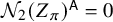 $\mathcal {N}_2(Z_\pi )^{\mathsf {A}}=0$
, and hence neither weight
$\mathcal {N}_2(Z_\pi )^{\mathsf {A}}=0$
, and hence neither weight
 $1$
or
$1$
or
 $t_3$
can come up in the character. The symplectic form is
$t_3$
can come up in the character. The symplectic form is
 $\mu _r$
-invariant, so it matches
$\mu _r$
-invariant, so it matches
 $\mu _r$
-invariant weights with
$\mu _r$
-invariant weights with
 $\mu _r$
-invariant weights. Here, we used that
$\mu _r$
-invariant weights. Here, we used that
 $\mu _r$
only acts on the first two coordinates. Using
$\mu _r$
only acts on the first two coordinates. Using
 $\mathcal {N}_2(Z_\pi )^{\mathsf {A}}=0$
and the matchings of weights by the symplectic form
$\mathcal {N}_2(Z_\pi )^{\mathsf {A}}=0$
and the matchings of weights by the symplectic form
 $\omega $
, we can match weights of
$\omega $
, we can match weights of
 $\mathcal {N}_2(Z_\pi )$
and
$\mathcal {N}_2(Z_\pi )$
and
 $t_3\mathcal {N}_2(Z_\pi )$
as follows
$t_3\mathcal {N}_2(Z_\pi )$
as follows

Since
 $\omega $
matches attracting and repelling weights in
$\omega $
matches attracting and repelling weights in
 $\mathcal {N}_2(Z_\pi )$
, attracting and repelling weights in
$\mathcal {N}_2(Z_\pi )$
, attracting and repelling weights in
 $t_3\mathcal {N}_2(Z_\pi )$
are also matched. This matches
$t_3\mathcal {N}_2(Z_\pi )$
are also matched. This matches
 $\mu _r$
-invariant weights with
$\mu _r$
-invariant weights with
 $\mu _r$
-invariant ones, so
$\mu _r$
-invariant ones, so
 $\mathsf {index}\left(((1-t_3)\mathcal {N}_2(Z_\pi ))^{\mu _r}\right)=0$
.
$\mathsf {index}\left(((1-t_3)\mathcal {N}_2(Z_\pi ))^{\mu _r}\right)=0$
.
The above result allows us to adjust the weight operator in the argument of [Reference Young39] and compute the limit of the generating series to finish the proof of Theorem 5.1. We recall now the setup of [Reference Young39], which is based on the setup in [Reference Okounkov30, Appendix A]. We consider a plane partition as a collection of slices, which are partitions
 $\{(a,b)\in \mathbb {Z}_{\geq 0}^2\ |\ (a+k,a,b)\in \pi \}$
consisting of the boxes with a fixed
$\{(a,b)\in \mathbb {Z}_{\geq 0}^2\ |\ (a+k,a,b)\in \pi \}$
consisting of the boxes with a fixed
 $i_1-i_2=k$
. With our specific
$i_1-i_2=k$
. With our specific
 $\mu _r$
-action a colored plane partition is then sliced into monochrome slices. This is pictured in Figure 2 below.
$\mu _r$
-action a colored plane partition is then sliced into monochrome slices. This is pictured in Figure 2 below.
Slicing of a
 $\mu _3$
-colored plane partition.
$\mu _3$
-colored plane partition.
This slicing can be used for counting by starting with empty partitions on the right and left side and iteratively applying operators, which give weighted sums of possible next slices moving inwards. We explain now how to formally set this up. We work in the charge-zero subspace of the infinite wedge space
 $\big (\bigwedge ^{\infty /2}\big )_0V$
, where V is a vector space with a basis labelled by the elements of
$\big (\bigwedge ^{\infty /2}\big )_0V$
, where V is a vector space with a basis labelled by the elements of
 $\mathbb {Z}+\frac {1}{2}$
. The vector space
$\mathbb {Z}+\frac {1}{2}$
. The vector space
 $\big (\bigwedge ^{\infty /2}\big )_0V$
has an orthonormal basis given by partitions
$\big (\bigwedge ^{\infty /2}\big )_0V$
has an orthonormal basis given by partitions ![]() .Footnote 2
.Footnote 2
There are operators
 $$ \begin{align*} \Gamma_\pm(x) = \mathrm{exp}\left(\sum_l \frac{x^l}{l}\alpha_{\pm l}\right) \end{align*} $$
acting on
 $\big (\bigwedge ^{\infty /2}\big )_0V$
, which act on a partition
$\big (\bigwedge ^{\infty /2}\big )_0V$
, which act on a partition ![]() by giving a weighted sum of possible partitions in the next smaller/bigger slice of a plane partition if the current one is
by giving a weighted sum of possible partitions in the next smaller/bigger slice of a plane partition if the current one is
 $\lambda $
.
$\lambda $
.
To compute the partition function, we consider weight operators
whose role it will be to count the contribution to the partition function of each slice. We now modify the argument as follows. In the limit of the equivariant parameters specified in (35), by Proposition 5.4, each slice
 $\lambda $
has a fixed contribution
$\lambda $
has a fixed contribution
 $1$
if the slice doesn’t have color
$1$
if the slice doesn’t have color
 $0$
, as only the boxes in
$0$
, as only the boxes in
 $\pi ^G$
contribute, and the slices of color
$\pi ^G$
contribute, and the slices of color
 $0$
have a fixed contribution
$0$
have a fixed contribution
 $$ \begin{align*} \begin{aligned} (-1)^{\lvert\lambda\rvert}(-\kappa^{1/2})^{\lvert\lambda\rvert}, &\mathrm{if }i_2\geq i_1,\\ (-1)^{\lvert\lambda\rvert}(-\kappa^{1/2})^{-\lvert\lambda\rvert}, &\mathrm{if }i_2< i_1. \end{aligned} \end{align*} $$
Here multiplied by the additional sign
 $(-1)^{\lvert \lambda \rvert }$
. This comes from the sign
$(-1)^{\lvert \lambda \rvert }$
. This comes from the sign
 $(-1)^{n_0}$
in the contribution of each partition, which comes from our definition of the twisted virtual structure sheaf and is usually manually introduced, as discussed in Remark 4.4. Since we consider slices
$(-1)^{n_0}$
in the contribution of each partition, which comes from our definition of the twisted virtual structure sheaf and is usually manually introduced, as discussed in Remark 4.4. Since we consider slices
 $\lambda $
with fixed
$\lambda $
with fixed
 $i_1-i_2$
this contribution is well-defined for each slice. We use this to define an additional equivariant limit weight operator
$i_1-i_2$
this contribution is well-defined for each slice. We use this to define an additional equivariant limit weight operator
We can now use the operators to define
 $$ \begin{align*} \bar{A}_\pm(x) = \Gamma_\pm(x) Q_{r-1} \cdots \Gamma_\pm(x) Q_1 \Gamma_\pm(x)K_\pm Q_0, \end{align*} $$
so that
computes the desired limit of the partition function, where
 $\phi $
denotes the empty partition. To compute this partition function, we want to compute the commutators of the operators involved and then reorder them.
$\phi $
denotes the empty partition. To compute this partition function, we want to compute the commutators of the operators involved and then reorder them.
Note that we wrote an infinite product of operators, which should be interpreted as follows. For any given finite order, we can make this a finite product of operators, such that (36) computes the limit generating series up to that given finite order. More precisely, if we want to compute all terms of
 $\overrightarrow {\mathsf {Z}}([\mathbb {C}^3/\mu _r],\mathbf {q})$
with
$\overrightarrow {\mathsf {Z}}([\mathbb {C}^3/\mu _r],\mathbf {q})$
with
 $\sum _i n_i\leq N$
for some N, then all colored plane partitions we have to consider have at most N boxes. In terms of the slicing shown in Figure 2, there are hence at most
$\sum _i n_i\leq N$
for some N, then all colored plane partitions we have to consider have at most N boxes. In terms of the slicing shown in Figure 2, there are hence at most
 $\left\lceil \frac {N}{2}\right\rceil +1$
slices on each side of the diagonal. Each operator
$\left\lceil \frac {N}{2}\right\rceil +1$
slices on each side of the diagonal. Each operator
 $\bar {A}_\pm (x)$
adds r slices, so that in (36) we only need to consider
$\bar {A}_\pm (x)$
adds r slices, so that in (36) we only need to consider
 $\left\lceil \frac {1}{r}\left(\left\lceil \frac {N}{2}\right\rceil +1\right)\right\rceil $
factors of
$\left\lceil \frac {1}{r}\left(\left\lceil \frac {N}{2}\right\rceil +1\right)\right\rceil $
factors of
 $\bar {A}_+(1)$
and
$\bar {A}_+(1)$
and
 $\bar {A}_-(1)$
each.
$\bar {A}_-(1)$
each.
Now we compute commutators of the various operators, so that we can reorder them in (36) to compute the generating series. The commutator
 $$ \begin{align} \left[\Gamma_+(a),\Gamma_-(b)\right] = \frac{1}{1-ab} \end{align} $$
was already computed in [Reference Young39, Lemma 3.3]. Moreover, Young computes
 $$ \begin{align*} \Gamma_+(x)Q_i=Q_i\Gamma_+(xq_i),\quad Q_i\Gamma_-(x)=\Gamma_-(xq_i)Q_i. \end{align*} $$
Using the same formula [Reference Young39, (4)], we can similarly compute
 $$ \begin{align*} \Gamma_+(x)K_+=K_+\Gamma_+\left(x\kappa^{1/2}\right),\quad K_-\Gamma_-(x)=\Gamma_-\left(x\kappa^{-1/2}\right)K_-. \end{align*} $$
Finally, by definition, the operators
 $Q_i$
and
$Q_i$
and
 $K_\pm $
commute with each other. Writing
$K_\pm $
commute with each other. Writing
 $q=q_0\cdots q_{r-1}$
and
$q=q_0\cdots q_{r-1}$
and
 $Q=Q_0\cdots Q_{r-1}$
, we can then rewrite
$Q=Q_0\cdots Q_{r-1}$
, we can then rewrite
 $\bar {A}_\pm (x)$
as follows.
$\bar {A}_\pm (x)$
as follows.
 $$ \begin{align*} \bar{A}_+(x) =& QK_+\Gamma_+\left(xq\kappa^{1/2}\right)\Gamma_+\left(xq_{[0,r-2]}\kappa^{1/2}\right)\cdots\Gamma_+\left(xq_0\kappa^{1/2}\right),\\ \bar{A}_-(x) =& \Gamma_-(x)\Gamma_-\left(xq_{r-1}\right)\cdots \Gamma_-\left(xq_{[2,r-1]}\right)\Gamma_-\left(xq_{[1,r-1]}\right)K_-Q. \end{align*} $$
We set
 $$ \begin{align*} A_+(x) :=& \ \Gamma_+\left(xq\kappa^{1/2}\right)\Gamma_+\left(xq_{[0,r-2]}\kappa^{1/2}\right)\cdots\Gamma_+\left(xq_0\kappa^{1/2}\right),\\ A_-(x) :=&\ \Gamma_-(x)\Gamma_-\left(xq_{r-1}\right)\cdots \Gamma_-\left(xq_{[2,r-1]}\right)\Gamma_-\left(xq_{[1,r-1]}\right). \end{align*} $$
Now iteratively using the commutators of
 $\Gamma _\pm $
from (37) we can compute
$\Gamma _\pm $
from (37) we can compute
 $$ \begin{align} A_+(x)A_-(y)=&\ \Gamma_+\left(xq_{[0,r-1]}\kappa^{1/2}\right)\Gamma_+\left(xq_{[0,r-2]}\kappa^{1/2}\right)\cdots\Gamma_+\left(xq_{[0,0]}\kappa^{1/2}\right)\cdot\nonumber\\ &\Gamma_-\left(y\frac{q}{q_{[0,r-1]}}\right)\Gamma_-\left(y\frac{q}{q_{[0,r-2]}}\right)\cdots \Gamma_-\left(y\frac{q}{q_{[0,1]}}\right)\Gamma_-\left(y\frac{q}{q_{[0,0]}}\right)\nonumber\\ =&\ A_-(y)A_+(x) \prod_{i,j=0}^{r-1}\left(1-xyq\frac{q_{[0,i]}}{q_{[0,j]}}\kappa^{1/2}\right)^{-1}. \end{align} $$
To simplify notation, we write
 $$ \begin{align*} C_r(x,y) := \prod_{i,j=0}^{r-1}\left(1-xyq\frac{q_{[0,i]}}{q_{[0,j]}}\kappa^{1/2}\right)^{-1}. \end{align*} $$
Now we can compute the partition function in the same way as [Reference Young39]. Note that as a product of
 $\Gamma _\pm $
, moving Q and
$\Gamma _\pm $
, moving Q and
 $K_\pm $
past the
$K_\pm $
past the
 $A_\pm $
works in the same way as simply for
$A_\pm $
works in the same way as simply for
 $\Gamma _\pm $
. After moving them to the outside, they act trivially on the empty partition.
$\Gamma _\pm $
. After moving them to the outside, they act trivially on the empty partition.

Now we can move the operators
 $A_\pm $
past each other using (38) to get
$A_\pm $
past each other using (38) to get

where we used that the operators
 $A_\pm $
act trivially on the empty partition
$A_\pm $
act trivially on the empty partition ![]() and
and ![]() , as in [Reference Young39, p. 14]. Now we can simplify this expression using standard formulas for the plethystic exponential. These formulas can be derived similar to the proof of Lemma 3.20. They are also discussed in [Reference Davison, Ongaro and Szendrői15, p. 4]. We compute
, as in [Reference Young39, p. 14]. Now we can simplify this expression using standard formulas for the plethystic exponential. These formulas can be derived similar to the proof of Lemma 3.20. They are also discussed in [Reference Davison, Ongaro and Szendrői15, p. 4]. We compute
 $$ \begin{align} \overrightarrow{\mathsf{Z}}\left([\mathbb{C}^3/\mu_r],\mathbf{q}\right) =& \prod_{a,b=0}^{\infty} \prod_{i,j=0}^{r-1}\left(1-q^{a+b+1}\frac{q_{[0,i]}}{q_{[0,j]}}\kappa^{\frac{i-j+1}{2}}\right)^{-1}\nonumber\\ =&\prod_{i,j=0}^{r-1}\mathrm{PExp}\,\left(\frac{\kappa^{1/2}q}{(1-\kappa^{1/2}q)(1-\kappa^{-1/2}q)}\frac{q_{[0,i]}}{q_{[0,j]}}\right)\nonumber\\ =&\ \mathrm{PExp}\,\left(\frac{-\kappa^{1/2}}{[\kappa^{1/2}q][\kappa^{1/2}q^{-1}]}\sum_{i,j=0}^{r-1}\frac{q_{[0,i]}}{q_{[0,j]}}\right). \end{align} $$
By splitting into parts with
 $i=j$
,
$i=j$
,
 $i<j$
, and
$i<j$
, and
 $i>j$
, we see that
$i>j$
, we see that
 $$ \begin{align*} \sum_{i,j=0}^{r-1}\frac{q_{[0,i]}}{q_{[0,j]}}=r+\sum_{0< i \leq j < r} q_{[i,j]}+q_{[i,j]}^{-1}, \end{align*} $$
so that (39) is exactly the desired limit
 $$ \begin{align*} \mathrm{PExp}\,\left(\frac{-\kappa^{1/2}}{[\kappa^{1/2}q][\kappa^{1/2}q^{-1}]}\left(r+\sum_{0< i \leq j < r} q_{[i,j]}+q_{[i,j]}^{-1}\right)\right) \end{align*} $$
of
 $\mathrm {PExp}\left(\mathsf {F}_r(q)+\mathsf {F}_r^{\mathrm {col}}(q_0,\dots ,q_{r-1})\right)$
. This determines the functions
$\mathrm {PExp}\left(\mathsf {F}_r(q)+\mathsf {F}_r^{\mathrm {col}}(q_0,\dots ,q_{r-1})\right)$
. This determines the functions
 $h_{\mathbf {n}}$
in Proposition 5.2 by rigidity, see Lemma 5.3, completing the proof of Theorem 5.1.
$h_{\mathbf {n}}$
in Proposition 5.2 by rigidity, see Lemma 5.3, completing the proof of Theorem 5.1.
A Quotient DM stacks
We state and prove a few simple facts about quotient DM stacks for use in Lemma 3.20. We consider the following setup. Let U be a scheme, and let
 $i:H\hookrightarrow G$
be finite groups acting on U, such that
$i:H\hookrightarrow G$
be finite groups acting on U, such that

commutes. We get the following induced morphism of DM stacks.
Proposition A.1. There is a morphism of DM stacks
 $$ \begin{align*} \eta:[U/H]\to [U/G], \end{align*} $$
induced by the inclusion
 $i:H\hookrightarrow G$
.
$i:H\hookrightarrow G$
.
Proof. An object of
 $[U/G]$
over a scheme T is a principal G-bundle
$[U/G]$
over a scheme T is a principal G-bundle
 $P\to T$
and a G-equivariant morphism
$P\to T$
and a G-equivariant morphism
 $P\to U$
. The morphism
$P\to U$
. The morphism
 $\eta $
is then concretely given by
$\eta $
is then concretely given by
 $$ \begin{align*} \left(T,P\to T,P\xrightarrow[H]{} U\right)\mapsto \left(T, G\times_H P, G\times_H P \xrightarrow[G]{} U\right). \end{align*} $$
Here ![]() with the anti-diagonal H-action
with the anti-diagonal H-action
 $h\cdot (g,p)=(gh,h^{-1}p)$
, and
$h\cdot (g,p)=(gh,h^{-1}p)$
, and
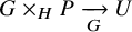 $G\times _H P \xrightarrow [G]{} U$
is the composition
$G\times _H P \xrightarrow [G]{} U$
is the composition
 $\mu _G\circ \left(\mathrm {id}\times (P\xrightarrow [H]{} U)\right)$
, which descends to
$\mu _G\circ \left(\mathrm {id}\times (P\xrightarrow [H]{} U)\right)$
, which descends to
 $G\times _H P$
as it is H-invariant.
$G\times _H P$
as it is H-invariant.
The pushforward along this morphism is just the induced representation construction.
Proposition A.2. Let
 $n=[G:H]$
and take a full set of representatives
$n=[G:H]$
and take a full set of representatives
 $g_1,\dots ,g_n$
of left cosets in
$g_1,\dots ,g_n$
of left cosets in
 $G/H$
. Given an H-equivariant sheaf
$G/H$
. Given an H-equivariant sheaf
 $\mathcal {E}$
on U, we have
$\mathcal {E}$
on U, we have
 $$ \begin{align*} \eta_* \mathcal{E} \cong \bigoplus_{i=1}^n g_i \mathcal{E} \end{align*} $$
as G-equivariant sheaves on U.
Proof. We consider the following cartesian diagram [Reference Alper1, Section 2.3.7]

where
 $\pi _G$
is the quotient morphism
$\pi _G$
is the quotient morphism
 $U\to [U/G]$
. All morphisms are H-equivariant with respect to H acting via
$U\to [U/G]$
. All morphisms are H-equivariant with respect to H acting via
 $\mu _H$
on U on the left side, acting anti-diagonally on
$\mu _H$
on U on the left side, acting anti-diagonally on
 $G\times U$
, and trivially on U and
$G\times U$
, and trivially on U and
 $[U/G]$
on the right side. Quotienting by H then gives us the cartesian diagram
$[U/G]$
on the right side. Quotienting by H then gives us the cartesian diagram

 $\eta _*\mathcal {E}$
as a G-equivariant sheaf on U is just
$\eta _*\mathcal {E}$
as a G-equivariant sheaf on U is just
 $\pi _G^*\eta _*\mathcal {E}$
with its natural G-equivariant structure induced by the cartesian diagram (40). By the cartesian diagram (41), this is isomorphic to
$\pi _G^*\eta _*\mathcal {E}$
with its natural G-equivariant structure induced by the cartesian diagram (40). By the cartesian diagram (41), this is isomorphic to
 $p_2^*\mathcal {E}$
, with its natural G-equivariant structure, pushed forward along the G-equivariant morphism
$p_2^*\mathcal {E}$
, with its natural G-equivariant structure, pushed forward along the G-equivariant morphism
 $\bar {\eta }$
.
$\bar {\eta }$
.
As
 $g_1,\dots ,g_n$
is a full set of representatives, any
$g_1,\dots ,g_n$
is a full set of representatives, any
 $g\in G$
has a presentation as
$g\in G$
has a presentation as
 $g=g_{i(g)}h(g)$
. This gives us a natural isomorphism
$g=g_{i(g)}h(g)$
. This gives us a natural isomorphism
 $$ \begin{align*} G\times_H U \xrightarrow{\sim} \bigsqcup_{i=1}^n g_i U,\ [g,u]\mapsto g_{i(g)} \left(h(g)\cdot u\right). \end{align*} $$
Again using that
 $g_1,\dots ,g_n$
is a full set of representatives, for any
$g_1,\dots ,g_n$
is a full set of representatives, for any
 $g\in G$
and
$g\in G$
and
 $g_i$
, there exists a
$g_i$
, there exists a
 $j(i,g)$
and an
$j(i,g)$
and an
 $h(i,g)\in H$
, such that
$h(i,g)\in H$
, such that
 $gg_i = g_{j(i,g)}h(i,g)$
. The above isomorphism induces the G-action
$gg_i = g_{j(i,g)}h(i,g)$
. The above isomorphism induces the G-action
 $g\cdot g_i u = g_{j(i,g)} (h(i,g)\cdot u)$
on the right-hand side.
$g\cdot g_i u = g_{j(i,g)} (h(i,g)\cdot u)$
on the right-hand side.
Under the above isomorphism,
 $\bar {\eta }$
becomes just the action morphism
$\bar {\eta }$
becomes just the action morphism
 $g_iU \to U, g_iu\mapsto g_i\cdot u$
on each component. Under this isomorphism
$g_iU \to U, g_iu\mapsto g_i\cdot u$
on each component. Under this isomorphism
 $p_2^*\mathcal {E}$
is just a copy of
$p_2^*\mathcal {E}$
is just a copy of
 $\mathcal {E}$
on every component. The natural G-equivariant structure of
$\mathcal {E}$
on every component. The natural G-equivariant structure of
 $p_2^*\mathcal {E}$
under this isomorphism is the following. For every
$p_2^*\mathcal {E}$
under this isomorphism is the following. For every
 $g\in G$
and
$g\in G$
and
 $g_i$
the action
$g_i$
the action
 $g: \bigsqcup _{i=1}^n g_i U \xrightarrow {\sim } \bigsqcup _{i=1}^n g_i U$
restricts to
$g: \bigsqcup _{i=1}^n g_i U \xrightarrow {\sim } \bigsqcup _{i=1}^n g_i U$
restricts to
 $h(i,g):g_i U \xrightarrow {\sim } g_{j(i,g)}U$
. On every component
$h(i,g):g_i U \xrightarrow {\sim } g_{j(i,g)}U$
. On every component
 $g_iU$
the isomorphism
$g_iU$
the isomorphism
 $g^*p_2^*\mathcal {E}\cong p_2^*\mathcal {E}$
is given by the isomorphism
$g^*p_2^*\mathcal {E}\cong p_2^*\mathcal {E}$
is given by the isomorphism
 $$ \begin{align*} h(i,g)^*\mathcal{E} \cong \mathcal{E}, \end{align*} $$
coming from the H-equivariant structure of
 $\mathcal {E}$
on U. Pushing this forward along
$\mathcal {E}$
on U. Pushing this forward along
 $\bar {\eta }$
yields exactly the desired isomorphism
$\bar {\eta }$
yields exactly the desired isomorphism
 $$ \begin{align*} \bar{\eta}_*p_2^* \mathcal{E} \cong \bigoplus_{i=1}^n g_i\mathcal{E}, \end{align*} $$
with the G-equivariant structure given by the isomorphisms
 $$ \begin{align} h(i,g)^*\left(g_{j(i,g)}\mathcal{E}\right) \cong g_i\mathcal{E}. \end{align} $$
Note that the
 $g_i$
in
$g_i$
in
 $\bigoplus _{i=1}^n g_i\mathcal {E}$
are purely formal for tracking the various copies of
$\bigoplus _{i=1}^n g_i\mathcal {E}$
are purely formal for tracking the various copies of
 $\mathcal {E}$
.
$\mathcal {E}$
.
Acknowledgments
I would like to thank my supervisor Jørgen Rennemo for many helpful discussions about this project, and for sharing and explaining an early draft of [Reference Kool and Rennemo22, Reference Vold Rennemo33], which inspired parts of this work. I would also like to thank Martijn Kool, Nick Kuhn, and Reinier Schmiermann for helpful discussions related to this project.
Competing interests
The author has no competing interests to declare.
Funding statement
None.
Data availability statement
There is not data and hence this is not applicable. A statement about how to access data, code and other materials allowing users to understand, verify and replicate findings – for example, Replication data and code can be found in Harvard Dataverse: https://doi.org/link.
Ethical standards
The research meets all ethical guidelines, including adherence to the legal requirements of the study country.


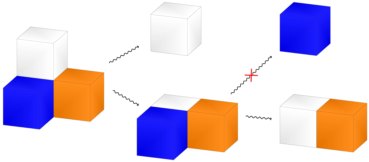

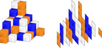


 Open access