


A growing number of social science studies use surveys to analyze the causal effect of major events on respondent beliefs, emotions, attitudes, or preferences. These events include political debates (Brady and Johnston, Reference Brady, Johnston, Brady and Johnston2006), voter outreach campaigns (Kalla and Broockman, Reference Kalla and Broockman2022), protests (Reny and Newman, Reference Reny and Newman2021), terrorist attacks (Breton and Eady, Reference Breton and Eady2022), sports competitions (Gläßel et al., Reference Gläßel, Scharpf and Edwards2025), announcements of pandemic restrictions (Eggers and Harding, Reference Eggers and Harding2022), and high-level state visits (Goldsmith, Horiuchi and Matush, Reference Goldsmith, Horiuchi and Matush2021). Since 2015, the APSR, AJPS, and JOP alone have published more than 30 such studies.Footnote 1 Sometimes researchers intentionally sample respondents before and after an event. Other times they examine events that co-occurred with survey fieldwork, splitting the sample into pre-event and post-event periods post-hoc. Despite the seemingly straightforward nature of these pre/post-event comparisons, various types of bias can weaken causal inference (Muñoz, Falcó-Gimeno and Hernández, Reference Muñoz, Falcó-Gimeno and Hernández2020). For instance, even if respondents are randomly sampled from the population of interest before and after the event, different non-response dynamics in each period can lead to systematic differences between these groups (Muñoz, Falcó-Gimeno and Hernández, Reference Muñoz, Falcó-Gimeno and Hernández2020).
We formalize the pre/post-event survey approach to distinguish biases that can arise in these event-based designs. We develop our analysis using the potential outcomes framework (Rubin, Reference Rubin2005; Hainmueller, Hopkins and Yamamoto, Reference Hainmueller, Hopkins and Yamamoto2014; Keele, Reference Keele2015; Broockman, Kalla and Sekhon, Reference Broockman, Kalla and Sekhon2017; Caughey et al., Reference Caughey, Dafoe, Xinran and Miratrix2023). We begin by considering a general case in which we make no assumption about the demographic comparability of the pre-event and post-event samples. This baseline model offers an initial way to think about many different pre/post-event survey designs, and its flexibility makes it particularly useful for modeling studies with unstructured or highly complex designs. Our formalization shows that bias in this baseline model can arise from four main sources: demographic differences between Wave 1 and 2 respondents, temporal factors, anticipation factors, and differential misreporting. We analyze these sources of bias and discuss steps researchers can take to mitigate them in various contexts.
Next, we extend our analysis to model three methods researchers employ to improve demographic balance between pre-event and post-event samples: quota sampling, rolling cross-sections, and panel designs. Our analysis sheds light on the strengths and weaknesses of each approach. For instance, we derive the conditions under which quota sampling reduces bias, which are not guaranteed to hold. In fact, we show that under certain conditions, quotas may increase bias. Similarly, we show that while rolling cross-sections should reduce imbalances between Wave 1 and 2 respondents, they are unlikely to eliminate these imbalances completely, and they complicate the overall bias term in other ways. Panels keep respondents constant across waves but risk panel conditioning, whereby the act of completing the survey in Wave 1 affects respondents’ answers in Wave 2 (Brady and Johnston, Reference Brady, Johnston, Brady and Johnston2006). This could result in attenuation bias if respondents tend to repeat their Wave 1 answers in Wave 2. To address this risk, we introduce a modified panel design—the dual randomized survey (DRS)—that combines some of the advantages of panels and rolling cross-sections.
Our bias formalization and novel research design complement recent advances in survey methods (e.g., Broockman, Kalla and Sekhon (Reference Broockman, Kalla and Sekhon2017); Morin-Chassé et al. (Reference Morin-Chassé, Bol, Stephenson and Labbé St-Vincent2017); Dafoe, Zhang and Caughey (Reference Dafoe, Zhang and Caughey2018); Donnelly and Pop-Eleches (Reference Donnelly and Pop-Eleches2018); Hanretty, Lauderdale and Vivyan (Reference Hanretty, Lauderdale and Vivyan2018); Miratrix et al. (Reference Miratrix, Sekhon, Theodoridis and Campos2018); Coppock (Reference Coppock2019); Caughey et al. (Reference Caughey, Berinsky, Chatfield, Hartman, Schickler and Sekhon2020); Schaffner (Reference Schaffner2022); Ben-Michael, Feller and Hartman (Reference Ben-Michael, Feller and Hartman2024); Munzert et al. (Reference Munzert, Ramirez-Ruiz, Barberá, Guess and Yang2024)). Most directly, we build on the work of Muñoz, Falcó-Gimeno and Hernández (Reference Muñoz, Falcó-Gimeno and Hernández2020) on unexpected events during surveys by providing a more comprehensive formalization of the pre/post-event survey framework and filling analytical gaps in places where their conclusions are incomplete. In particular, our formalization accounts for anticipation bias around expected events and, by doing so, offers a unified analytical framework for both expected and unexpected events. This advancement matters because many events cannot easily be categorized as expected or unexpected, as we explain in the next section. In addition, our formalized framework allows us to account for bias from measurement error in survey responses. Our contribution is therefore a broadly applicable toolkit for a wide range of political science studies that estimate the causal impact of events through surveys.
1. Can events be categorized as “expected” or “unexpected”?
In their widely cited article on the causal impact of unexpected events on survey responses, Muñoz, Falcó-Gimeno and Hernández (Reference Muñoz, Falcó-Gimeno and Hernández2020, 187) suggest that expected events should not be studied using before/after survey comparisons because event anticipation may affect respondents’ pre-event responses, biasing results. Notably, however, their examples of expected and unexpected events demonstrate the problematic nature of this dichotomy. They suggest that sports results are unexpected and election results are expected (Muñoz, Falcó-Gimeno and Hernández, Reference Muñoz, Falcó-Gimeno and Hernández2020, 186-87). In both cases, event timing is expected, whereas event outcome is largely unknown. In turn, event anticipation may bias the before/after comparison in both contexts. Many events are similar in this feature—their timing is known, but their outcome is uncertain: political debates and speeches, international meetings and summits, major court rulings, and scheduled announcements of important policy decisions. In fact, fully expected events, in which both event timing and outcome are certain to the public beforehand, are quite rare in political science.
Fully unexpected events are also rare. Terror attacks, mass shootings, the onset of war, and political protests constitute cases where respondents likely recognize the possibility that such an event could occur, even if they do not know whether it will nor its precise timing. This general awareness may influence respondents’ political beliefs and attitudes prior to the event. These types of events are still plausibly categorized as unexpected, insofar that they may be significantly lower salience to respondents immediately before the event takes place. That said, it is still more appropriate to conceptualize expected and unexpected events along a broad continuum rather than dichotomous in nature.
If most events are expected in some ways and unexpected in others, the anticipation bias Muñoz, Falcó-Gimeno and Hernández (Reference Muñoz, Falcó-Gimeno and Hernández2020) highlight is important to define precisely and consider carefully in almost all before/after survey contexts. In the next section, we offer a clear mathematical definition of anticipation bias directly connected to the event in question, thereby distinguishing it from background levels of event anticipation. This allows us to develop a unified analytical framework that applies to any event regardless of its degree of unexpectedness. Our framework reveals other novel insights, discussed in subsequent sections.
2. The baseline model: disaggregating potential sources of bias
We model the theoretical framework for our baseline model as follows. Each individual who a researcher (or survey firm) attempts to contact in Wave 2 has some truthful response to question  $k$ of the survey, which we denote as $y_{ikt}$. This $y_{ikt}$ value represents individual $i$’s true and honest response to question $k$ in the world where the event happened. The $t$ in the subscript stands for “treatment,” which we conceptualize as living through the event. Additionally, in theory, all individuals have a truthful response to question $k$ in the counterfactual world where the event did not happen. We will discuss what we mean by this “counterfactual world” in more detail shortly, as there may be multiple possibilities that have different implications for analysis. For example, an event being postponed at the last minute is a different counterfactual than an event never being scheduled. For now, we assume that some well-defined counterfactual exists and denote individual $i$’s hypothetical truthful response in this counterfactual world as $y_{ikc}$.
Therefore, each individual in Wave 2 has an (unobservable) individual-level treatment effect for question  $k$:
$k$:
 \begin{align*}
\tau_{ik} & =y_{ikt}-y_{ikc} \nonumber
\end{align*}
\begin{align*}
\tau_{ik} & =y_{ikt}-y_{ikc} \nonumber
\end{align*}Notably, this conceptualization considers individuals who did not witness the event as “treated.” The event might influence them indirectly (through peers or the news) or not at all.
An alternative conceptualization would consider these individuals untreated, implying a counterfactual in which they had been exposed to the event (Muñoz, Falcó-Gimeno and Hernández, Reference Muñoz, Falcó-Gimeno and Hernández2020). This approach presents conceptual challenges because it necessitates defining what constitutes event exposure—would watching the event on TV for just one minute qualify? Furthermore, this ambiguity makes the treatment non-binary, as individuals can experience the event in various ways and to varying degrees. Therefore, we conceptualize treatment as having lived through the event, which implies null effects for those unaffected (and possibly even unaware) of the event. The alternative approach of counting such individuals as untreated may be appropriate in some contexts, in particular when researchers use difference-in-differences to compare “exposed” to “unexposed” individuals. However, this conceptualization introduces ambiguities that our definitional approach avoids.
Thus, using our framework researchers cannot observe  $y_{ikc}$. They also do not observe $y_{ikt}$ directly but instead measure it as individual $i$’s observed response to question $k$ on the survey, which we denote $y_{ikto}$. The values $y_{ikt}$ and $y_{ikto}$ might be equivalent or might differ due to social desirability bias, self-esteem bias, individual $i$ not reading the survey question carefully, or some other reason that causes misreporting.
Let us denote the number of people in the population of interest by  $N$ and the number who complete the survey in Wave 2 by $n_a$ (where “a” stands for “after”). Furthermore, we denote whether individual $i$ completed the survey in Wave 2 by the variable $r_{ia}\in\{0,1\}$. The first causal parameter we might be interested in is the average treatment effect for the population of interest:
 \begin{align*}
\bar{\tau}_{k}=\tfrac{1}{N}\sum_{i=1}^{N} \left(y_{ikt}-y_{ikc}\right) \nonumber
\end{align*}
\begin{align*}
\bar{\tau}_{k}=\tfrac{1}{N}\sum_{i=1}^{N} \left(y_{ikt}-y_{ikc}\right) \nonumber
\end{align*} We cannot directly compute this quantity, since we only observe the  $y_{ikto}$ values for Wave 2 respondents. Therefore, a second causal parameter we have more information on is the average causal effect of the event for Wave 2 respondents.
 \begin{align*}
\bar{\tau}_{k|r_a=1}=\tfrac{1}{n_a}\sum_{i=1}^{n_a} \left(y_{ikt|r_a=1}-y_{ikc|r_a=1}\right) \nonumber
\end{align*}
\begin{align*}
\bar{\tau}_{k|r_a=1}=\tfrac{1}{n_a}\sum_{i=1}^{n_a} \left(y_{ikt|r_a=1}-y_{ikc|r_a=1}\right) \nonumber
\end{align*} Given the lack of information about  $y_{ikt|r_a=0}$ values, we focus on estimating $\bar{\tau}_{k|r_a=1}$. Since researchers observe all $y_{ikto|r_a=1}$ values, they can use these as a measure of the $y_{ikt|r_a=1}$ values. Without a similar measure for the counterfactual $y_{ikc|r_a=1}$ values, they must estimate the average of $y_{ikc|r_a=1}$. With the exception of panel designs, the standard estimator is the average response to the same question from a survey conducted prior to the event (Wave 1) on a different group of $n_b$ individuals (where “b” stands for “before”). We can denote whether individual $i$ completed the survey in Wave 1 with the variable $r_{ib}\in\{0,1\}$. Furthermore, we can denote individual $i$’s Wave 1 observed response to question $k$ as $y_{ikbo}$. Thus, we have
 \begin{align*}
\hat{\tau}_{k|r_a=1}=\tfrac{1}{n_a}\sum_{i=1}^{n_a} y_{ikto|r_a=1}-\hat{y}_{ikc|r_a=1} \nonumber
\end{align*}
\begin{align*}
\hat{\tau}_{k|r_a=1}=\tfrac{1}{n_a}\sum_{i=1}^{n_a} y_{ikto|r_a=1}-\hat{y}_{ikc|r_a=1} \nonumber
\end{align*}where
 \begin{align*}
\hat{y}_{ikc|r_a=1}=\tfrac{1}{n_b} \sum_{i=1}^{n_b} y_{ikbo|r_b=1} \nonumber
\end{align*}
\begin{align*}
\hat{y}_{ikc|r_a=1}=\tfrac{1}{n_b} \sum_{i=1}^{n_b} y_{ikbo|r_b=1} \nonumber
\end{align*} In this second estimator, note that  $i$ indexes the set of individuals who completed the survey prior to the event (in Wave 1).
We can formally define average measurement error in the two waves as follows:
 \begin{align*}
\bar{\epsilon}_{kt|r_a=1}=\tfrac{1}{n_a}\sum_{i=1}^{n_a} y_{ikto|r_a=1}- \tfrac{1}{n_a}\sum_{i=1}^{n_a} y_{ikt|r_a=1} \nonumber
\end{align*}
\begin{align*}
\bar{\epsilon}_{kt|r_a=1}=\tfrac{1}{n_a}\sum_{i=1}^{n_a} y_{ikto|r_a=1}- \tfrac{1}{n_a}\sum_{i=1}^{n_a} y_{ikt|r_a=1} \nonumber
\end{align*}and
 \begin{align*}
\bar{\epsilon}_{kb|r_b=1}=\tfrac{1}{n_b}\sum_{i=1}^{n_b} y_{ikbo|r_b=1}- \tfrac{1}{n_b}\sum_{i=1}^{n_b} y_{ikb|r_b=1} \nonumber
\end{align*}
\begin{align*}
\bar{\epsilon}_{kb|r_b=1}=\tfrac{1}{n_b}\sum_{i=1}^{n_b} y_{ikbo|r_b=1}- \tfrac{1}{n_b}\sum_{i=1}^{n_b} y_{ikb|r_b=1} \nonumber
\end{align*} Lastly, we can consider one additional potential outcome: individual  $i$’s truthful Wave 1 response in the counterfactual world where the event did not happen.Footnote 2 We can denote this counterfactual outcome by $y_{ikbc}$. As we show in the Online Appendix (Section 2), introducing this potential outcome allows us to disaggregate the overall bias in the baseline model as follows:
Summary of key terms

Proposition 1. Bias in the baseline model can be written as
 \begin{equation}
Bias\left(\hat{\tau}_{k|r_a=1}\right)= Bias_{\mathbf{X}}\left(\hat{\tau}_{k|r_a=1}\right) + Bias_{\mathbf{T}}\left(\hat{\tau}_{k|r_a=1}\right) + Bias_{\mathbf{A}}\left(\hat{\tau}_{k|r_a=1}\right)+ Bias_{\mathbf{M}}\left(\hat{\tau}_{k|r_a=1}\right)
\end{equation}
\begin{equation}
Bias\left(\hat{\tau}_{k|r_a=1}\right)= Bias_{\mathbf{X}}\left(\hat{\tau}_{k|r_a=1}\right) + Bias_{\mathbf{T}}\left(\hat{\tau}_{k|r_a=1}\right) + Bias_{\mathbf{A}}\left(\hat{\tau}_{k|r_a=1}\right)+ Bias_{\mathbf{M}}\left(\hat{\tau}_{k|r_a=1}\right)
\end{equation}where
 \begin{align*}
& Bias_\mathbf{X}\left(\hat{\tau}_{k|r_a=1}\right)=\bar{y}_{ikb|r_a=1}- \bar{y}_{ikb|r_b=1} \text{(Demographic Bias)} \\
& Bias_{\mathbf{T}}\left(\hat{\tau}_{k|r_a=1}\right)=\bar{y}_{ikc|r_a=1}-\bar{y}_{ikbc|r_a=1} \text{(Temporal Bias)} \\
& Bias_{\mathbf{A}}\left(\hat{\tau}_{k|r_a=1}\right)=\bar{y}_{ikbc|r_a=1}-\bar{y}_{ikb|r_a=1} \text{(Anticipation Bias)} \\
& Bias_{\mathbf{M}}\left(\hat{\tau}_{k|r_a=1}\right)=\bar{\epsilon}_{kt|r_a=1}-\bar{\epsilon}_{kb|r_b=1} \text{(Differential Misreporting)}
\end{align*}
\begin{align*}
& Bias_\mathbf{X}\left(\hat{\tau}_{k|r_a=1}\right)=\bar{y}_{ikb|r_a=1}- \bar{y}_{ikb|r_b=1} \text{(Demographic Bias)} \\
& Bias_{\mathbf{T}}\left(\hat{\tau}_{k|r_a=1}\right)=\bar{y}_{ikc|r_a=1}-\bar{y}_{ikbc|r_a=1} \text{(Temporal Bias)} \\
& Bias_{\mathbf{A}}\left(\hat{\tau}_{k|r_a=1}\right)=\bar{y}_{ikbc|r_a=1}-\bar{y}_{ikb|r_a=1} \text{(Anticipation Bias)} \\
& Bias_{\mathbf{M}}\left(\hat{\tau}_{k|r_a=1}\right)=\bar{\epsilon}_{kt|r_a=1}-\bar{\epsilon}_{kb|r_b=1} \text{(Differential Misreporting)}
\end{align*} Researchers are typically interested in the average treatment effect for the broader population ( $\bar{\tau}_{k}$). For this target parameter, we would add one more bias term to Equation 1 to represent the difference between the average treatment effect for Wave 2 respondents and the average treatment effect for the population: $\bar{\tau}_{k|r_a=1}-\bar{\tau}_{k}$. Substantively, this expression would capture the potential bias caused by the average treatment effect for Wave 2 respondents differing from the average treatment effect for the overall population. We will not include this additional term in our baseline model to avoid conflating internal and external validity. However, in our extensions that follow, readers can draw the link to external validity by adding a simple term to the bias equations that accounts for such potential heterogeneous treatment effects. For a formalization of this link to external validity, see the Online Appendix (Section 3).
Returning to internal validity, when estimating  $\bar{\tau}_{k|r_a=1}$, Equation 1 breaks the bias term into four additively separable components: bias from demographic differences between Wave 1 and 2 respondents, bias from temporal differences between Waves 1 and 2, bias from anticipation factors, and bias from differential measurement error in the two waves.
With events that respondents do not know the timing of beforehand, such as earthquakes and political scandals, the anticipation bias term should be negligible. This is because we have defined it formally in reference to the specific event and not merely to capture the possible impact of knowledge that such an event might occur. We do not posit a counterfactual world where such an event was entirely unexpected (e.g., Californians were not aware that an earthquake might happen) because such counterfactuals are often implausible. Therefore, the impact of this more general type of anticipation is commonly baked into pre/post-event survey designs and should be acknowledged by researchers when appropriate.
Researchers should also assess whether privately informed actors may have engaged in behavior that could have contaminated Wave 1 responses. For example, a politician anticipating imminent scandal may issue preemptive, reputational damage-control statements. Such strategic signaling can shift public attitudes before the disclosure, introducing anticipation bias despite respondents’ limited knowledge of the event.
Researchers might also look for evidence that some respondents anticipated the specific event. For example, researchers might check news reports and social media for indications that some people knew the specific event would or might happen. Researchers could also examine the pre-event data for trends that suggest anticipation. However, any observed trends might be driven by other factors, including other events (see also Malani and Reif (Reference Malani and Reif2015)). Therefore, the usefulness of this test would depend on context-specific factors that support the notion that an observed trend in pre-event data is best explained by anticipation.
For events that respondents know will occur at a precise time, whether the anticipation bias term formalized above is concerning depends on how researchers define the counterfactual. When researchers define the counterfactual as the world where the event was rescheduled at the last minute in a manner unlikely to impact respondents’ relevant beliefs and attitudes, the anticipation bias term should drop out because the event lead-up would be equivalent in both the real and counterfactual worlds. However, if researchers define the counterfactual as the world where the event was never scheduled, the lead-up in the counterfactual world could differ, possibly causing anticipation bias.
Ultimately, it is up to researchers to choose which counterfactual is most sensible given their study’s context. Although the “last-minute rescheduling” counterfactual minimizes concerns about anticipation bias, researchers may have substantive reasons for choosing a less neutral counterfactual, such as the event never being scheduled. In such cases, researchers might set the Wave 1 period to end a week or more before the event, which risks bias from temporal factors but could decrease possible bias from anticipation. Regardless of which counterfactual researchers choose, they can clarify their analyses by specifying their exact counterfactual, since this affects their sources of bias. Moreover, specifying the counterfactual helps ensure that study framing, theoretical discussion, and conclusions are consistent with research design and empirical analysis.
Researchers can take steps to minimize anticipation bias, but what about temporal bias? Muñoz, Falcó-Gimeno and Hernández (Reference Muñoz, Falcó-Gimeno and Hernández2020) suggest multiple strategies that could be used to address this type of bias. These include checking online search trends and print media for other salient events that might have co-occurred with the survey, considering whether the event was strategically timed, and inspecting the data for temporal trends. In particular, researchers can check if there were significant weather differences between Wave 1 and 2 that might have influenced respondents’ moods during survey completion. Temporal bias may be further mitigated by design choices, including fielding Wave 1 and 2 at the same time of day and the same day(s) of the week. Because it is impossible to rule out all possible types of temporal bias, researchers should acknowledge its potential impact on their results and advance their conclusions with caution.
Concerning bias from differential misreporting, researchers can consider whether the event itself or some other factor might have affected social desirability bias or another form of misreporting in Wave 2 (see McCauley et al. (Reference McCauley, Finkel, Neureiter and Belasco2022)). For instance, Singh and Tir (Reference Singh and Tir2023) find that threat-inducing violent events increase social desirability bias in survey responses across a range of contexts. Researchers can also consider whether respondents might have been more rushed to complete the survey in one of the two waves, either because of demographic differences between Wave 1 and 2 respondents or due to temporal differences between waves.
Can regression discontinuity (RD) reduce some of the aforementioned sources of bias by adjusting for temporal trends before and after the event? Unfortunately, RD faces several limitations in this setting. First, RD estimators require potential outcomes to be sufficiently smooth on both sides of the cut-point so that they can be modeled accurately with local linear regression or other smoothing techniques (see Calonico, Cattaneo and Titiunik (Reference Calonico, Cattaneo and Titiunik2014); Sekhon and Titiunik (Reference Sekhon and Titiunik2017)). However, demographic differences are likely to lack temporal smoothness. The types of people who complete surveys during the final hours of the workday likely systematically differ from those who answer surveys an hour or two after the workday ends. If researchers aggregate responses at the day level, we should also expect systematic differences between those who complete surveys on weekdays and weekends (also see Hausman and Rapson (Reference Hausman and Rapson2018, 539)). Simultaneous events also pose a threat to the smoothness requirement, possibly causing jumps or drops in the potential outcomes across time.
Furthermore, standard RD designs typically focus on scoring systems in which actors cannot precisely manipulate their scores. In fact, evidence that precise manipulation occurred is considered strong evidence against a regression discontinuity design (Caughey and Sekhon, Reference Caughey and Sekhon2011). In contrast, the timing of survey completion is typically precisely chosen, either by respondents themselves or by survey administrators (see also Hausman and Rapson (Reference Hausman and Rapson2018, 538)). Even in contexts where sorting around the cut-point might be unlikely, precise manipulation can still pose a problem for estimation by threatening smoothness in the potential outcomes on each side of the cut-point. Muñoz, Falcó-Gimeno and Hernández (Reference Muñoz, Falcó-Gimeno and Hernández2020) highlight other concerns with using regression discontinuity to study how events impact survey responses, including that the effects of events can take time to unfold, which differs from well-defined cut-points in standard RDs (see also Hausman and Rapson (Reference Hausman and Rapson2018, 545-46)).
Rather than turning to RD estimation, the strategies discussed in this section can mitigate concerns regarding bias in pre/post-event survey designs. In particular, temporal, anticipation, and differential misreporting biases may be alleviated with appropriate field strategies, design choices, and robustness checks. Demographic bias, on the other hand, presents a distinct set of challenges. In the next section, we analyze three approaches to reduce demographic bias. Our results clarify the extent to which these methods can reliably reduce bias for pre/post-event survey designs.
3. Comparing bias in the baseline model to bias in other designs
To what extent do quota sampling, rolling cross-sections, and panel designs reduce bias compared to our simple baseline model? We begin with the quota sampling method.
3.1. Quotas
Quota sampling can be executed in two ways. In the first, an event occurs during the fieldwork of a quota sample study, and the event is then used to distinguish Waves 1 and 2. In the second, researchers collect two different study waves pre/post-event, maintaining distinct quotas for each wave. The first scenario provides researchers limited leverage to assume comparability of pre/post-event samples. Some demographic quotas will likely fill faster than others due to ease-of-reach and other propensity to respond factors (Muñoz, Falcó-Gimeno and Hernández, Reference Muñoz, Falcó-Gimeno and Hernández2020, 192), meaning that some types of respondents will be concentrated toward the beginning of the fieldwork (in this case, Wave 1).Footnote 3 Therefore, the first scenario should be modeled with the flexible baseline approach, which does not make assumptions about the comparability of Wave 1 and 2 respondents. In contrast, in the second scenario, researchers directly attempt to improve comparability by using separate quotas administered before and after the event.
We now adapt our baseline model to more precisely fit this second quota sampling scenario. We can think of this scenario as similar to our baseline model except that we keep or drop potential respondents based on whether they help meet our demographic quotas in Waves 1 and 2. Let  $g_b$ denote the number of people in our Wave 1 quota group and $g_a$ denote the number of people in our Wave 2 quota group. Likewise, we exclude some people in Waves 1 and 2 based on quota constraints. Let $e_b$ and $e_a$ denote the number of people in Waves 1 and 2, respectively, who would have completed our survey but who we exclude due to quota constraints. In total, we then have $n_b=g_b+e_b$ individuals in Wave 1 and $n_a=g_a+e_a$ individuals in Wave 2 who would complete our survey if asked. We use $q_i\in\{0,1\}$ to denote whether individual $i$ is in our quota sample as opposed to the excluded group.
The causal parameter we estimate is the average treatment effect of the event on the Wave 2 quota group’s truthful responses to survey question  $k$:
$k$:
 \begin{align*}
\bar{\tau}_{k|r_a=1,q=1}=\tfrac{1}{g_a} \sum_{i=1}^{g_a} \left(y_{ikt|r_a=1,q=1}-y_{ikc|r_a=1,q=1}\right) \nonumber
\end{align*}
\begin{align*}
\bar{\tau}_{k|r_a=1,q=1}=\tfrac{1}{g_a} \sum_{i=1}^{g_a} \left(y_{ikt|r_a=1,q=1}-y_{ikc|r_a=1,q=1}\right) \nonumber
\end{align*} The statistic we use to estimate this parameter is the average difference between the reported answers of the  $g_a$ respondents who completed our survey in Wave 2 and the reported answers of the $g_b$ respondents who completed the survey in Wave 1.
 \begin{align*}
\hat{\tau}_{k|r_a=1,q=1}=\tfrac{1}{g_a}\sum_{i=1}^{g_a} y_{ikto|r_a=1,q=1}-\tfrac{1}{g_b}\sum_{i=1}^{g_b} y_{ikbo|r_b=1,q=1} \nonumber
\end{align*}
\begin{align*}
\hat{\tau}_{k|r_a=1,q=1}=\tfrac{1}{g_a}\sum_{i=1}^{g_a} y_{ikto|r_a=1,q=1}-\tfrac{1}{g_b}\sum_{i=1}^{g_b} y_{ikbo|r_b=1,q=1} \nonumber
\end{align*}We provide the full analysis of this design, including proofs of the propositions that follow, in the Online Appendix (Section 4). Proposition 2 establishes that the bias of the quota sampling approach can be written as the sum of biases from the demographic differences between Wave 1 and 2 respondents, temporal factors, anticipation factors, and differential misreporting.
Proposition 2. When researchers use separate quotas in Wave 1 and 2 to try to achieve balance between the pre-event and post-event groups, bias can be written as
 \begin{align*}
Bias\left(\hat{\tau}_{k|r_a=1,q=1}\right)= Bias_{\mathbf{X}}\left(\hat{\tau}_{k|r_a=1,q=1}\right) + Bias_{\mathbf{T}}\left(\hat{\tau}_{k|r_a=1,q=1}\right) + Bias_{\mathbf{A}}\left(\hat{\tau}_{k|r_a=1,q=1}\right) + Bias_{\mathbf{M}}\left(\hat{\tau}_{k|r_a=1,q=1}\right)
\end{align*}
\begin{align*}
Bias\left(\hat{\tau}_{k|r_a=1,q=1}\right)= Bias_{\mathbf{X}}\left(\hat{\tau}_{k|r_a=1,q=1}\right) + Bias_{\mathbf{T}}\left(\hat{\tau}_{k|r_a=1,q=1}\right) + Bias_{\mathbf{A}}\left(\hat{\tau}_{k|r_a=1,q=1}\right) + Bias_{\mathbf{M}}\left(\hat{\tau}_{k|r_a=1,q=1}\right)
\end{align*}where
 \begin{align*}
& Bias_\mathbf{X}\left(\hat{\tau}_{k|r_a=1,q=1}\right)=\bar{y}_{ikb|r_a=1,q=1}- \bar{y}_{ikb|r_b=1,q=1} \\
& Bias_{\mathbf{T}}\left(\hat{\tau}_{k|r_a=1,q=1}\right)=\bar{y}_{ikc|r_a=1,q=1}-\bar{y}_{ikbc|r_a=1,q=1}\\
& Bias_{\mathbf{A}}\left(\hat{\tau}_{k|r_a=1,q=1}\right)=\bar{y}_{ikbc|r_a=1,q=1}-\bar{y}_{ikb|r_a=1,q=1}\\
& Bias_{\mathbf{M}}\left(\hat{\tau}_{k|r_a=1,q=1}\right)=\bar{\epsilon}_{kt|r_a=1,q=1}-\bar{\epsilon}_{kb|r_b=1,q=1}
\end{align*}
\begin{align*}
& Bias_\mathbf{X}\left(\hat{\tau}_{k|r_a=1,q=1}\right)=\bar{y}_{ikb|r_a=1,q=1}- \bar{y}_{ikb|r_b=1,q=1} \\
& Bias_{\mathbf{T}}\left(\hat{\tau}_{k|r_a=1,q=1}\right)=\bar{y}_{ikc|r_a=1,q=1}-\bar{y}_{ikbc|r_a=1,q=1}\\
& Bias_{\mathbf{A}}\left(\hat{\tau}_{k|r_a=1,q=1}\right)=\bar{y}_{ikbc|r_a=1,q=1}-\bar{y}_{ikb|r_a=1,q=1}\\
& Bias_{\mathbf{M}}\left(\hat{\tau}_{k|r_a=1,q=1}\right)=\bar{\epsilon}_{kt|r_a=1,q=1}-\bar{\epsilon}_{kb|r_b=1,q=1}
\end{align*} This overall bias term is similar to the  $Bias(\hat{\tau}_{k|r_a=1})$ term in Section 2, except that it restricts the focus to our quota sample.
Does quota sampling reduce bias? Proposition 3 shows the conditions under which quotas reduce or amplify bias.
Proposition 3. Research designs using separate quotas in Waves 1 and 2 to try to improve balance reduce bias if and only if
 \begin{align*}
\bigg|Bias\left(\hat{\tau}_{k|r_a=1,q=1}\right)\bigg|& \lt \bigg|\left(\tfrac{g_a}{n_a}\right)Bias\left(\hat{\tau}_{k|r_a=1,q=1}\right) + \left(\tfrac{e_a}{n_a}\right)Bias\left(\hat{\tau}_{k|r_a=1,q=0}\right)+ \nonumber
\\ & \left(\tfrac{g_a}{n_a}-\tfrac{g_b}{n_b}\right)\left(\bar{y}_{ikbo|r_b=1,q=1}-\bar{y}_{ikbo|r_b=1,q=0}\right)\bigg| \nonumber
\end{align*}
\begin{align*}
\bigg|Bias\left(\hat{\tau}_{k|r_a=1,q=1}\right)\bigg|& \lt \bigg|\left(\tfrac{g_a}{n_a}\right)Bias\left(\hat{\tau}_{k|r_a=1,q=1}\right) + \left(\tfrac{e_a}{n_a}\right)Bias\left(\hat{\tau}_{k|r_a=1,q=0}\right)+ \nonumber
\\ & \left(\tfrac{g_a}{n_a}-\tfrac{g_b}{n_b}\right)\left(\bar{y}_{ikbo|r_b=1,q=1}-\bar{y}_{ikbo|r_b=1,q=0}\right)\bigg| \nonumber
\end{align*}When the inequality is flipped, quota sampling amplifies bias.
The first two expressions to the right of the inequality are the weighted average of the biases in the quota sample and the excluded group. The intuition is that we should expect quota sampling to increase bias when the bias in the excluded group is smaller than the bias in the quota group or when the bias terms for the two groups point in opposite directions and thus partially cancel each other out.
The final expression is a residual term that arises when  $Bias\left(\hat{\tau}_{k|r_a=1}\right)$ is separated into a weighted average of $Bias\left(\hat{\tau}_{k|r_a=1,q=1}\right)$ and $Bias\left(\hat{\tau}_{k|r_a=1,q=0}\right)$. This residual term can grow large when there is a notable difference between the proportion of Wave 1 and 2 individuals who are in the quota groups (rather than the excluded groups). In particular, this can happen when it is easier to find respondents to satisfy quotas in Wave 1 than in Wave 2. In such cases, quota sampling may increase bias if the weighted average and residual term point in opposite directions.
Canvassers having more trouble meeting quotas in Wave 2 than in Wave 1 is a plausible concern in some contexts. For example, the European Social Survey (ESS) allows discretionary subgroup-targeted survey enhancement, meaning that “[s]everal countries specifically target subgroups which are less cooperative, by restricting incentives to particular areas (e.g., the Russian Federation), allowing the interviewers to offer an (additional) incentive at the doorstep (e.g., Poland) and/or increasing incentives with re-issues (e.g., the Netherlands)” (Wuyts and Loosveldt, Reference Wuyts and Loosveldt2019, 79). The need for these targeted, discretionary survey enhancements suggests that certain quotas are significantly harder to fill and that if ESS conducted a second wave just days to weeks later, this need for enumerator discretion in subgroup recontacts and incentives may exacerbate bias on unobservables, even while demographic quotas appear balanced.
For general population surveys, discretionary incentive measures are typically not due to the absolute availability of subgroup respondents, but rather the additional effort required to convert non-respondents to respondents (Singer and Ye, Reference Singer and Cong2013, 116). This means that these efforts are likely to remain constant across waves. However, time-variant recontact measures and incentives remain an important consideration for researchers when surveying specific subpopulations or facing other sampling constraints. We discuss additional examples of how quota sampling can amplify bias in the Online Appendix (Section 4) that involve door-to-door, phone, and internet surveys. Given the potential of quota sampling to exacerbate bias, we consider it suboptimal to estimate the causal effects of events through surveys. This conclusion accords with the conventional view in statistics that quota sampling, despite its convenience, is unreliable for obtaining representative samples (e.g., see Bowling and Ebrahim (Reference Bowling and Ebrahim2005, 199); Freedman, Pisani and Purves (Reference Freedman, Pisani and Purves2007, 334-38); Yang and Banamah (Reference Yang and Banamah2014)).
3.2. Rolling cross-sections
Next, we examine the rolling cross-section design. Our analysis here can also be used to think about other similar designs, such as random-digit dialing or selecting a specific set of individuals and randomizing whether they are asked to complete the survey in Wave 1 or 2.
Researchers studying the impact of events using rolling cross-section data often take existing survey data from a lengthy rolling cross-section project lasting months and compare the responses just before and after a certain event (see Brady and Johnston (Reference Brady, Johnston, Brady and Johnston2006, 166)). For such cases, we will restrict our attention to the individuals surveyed in these two periods, labeling the period just before the event as Wave 1 and the period just after as Wave 2.
We conceptualize this design as beginning with an initial sample that includes a group of “always-responders” who would complete the survey in either wave, a group of “sometimes-responders” who would complete the survey only in Wave 1 or Wave 2 but not both, and a group of “never-responders” who would not complete the survey in either wave. We focus on the always-responders and sometimes-responders since never-responders are inaccessible to us.Footnote 4
Let  $n_w$ denote the total number of always-responders and sometimes-responders who could initially be asked to complete the survey in Waves 1 or 2. We again denote the number who complete the survey in each wave by $n_a$ (Wave 2) and $n_b$ (Wave 1). We can also denote the total number of always-responders in the sample by $n^*$. Furthermore, let $m_a$ represent the number of sometimes-responders who would only complete the survey in Wave 2 and $m_b$ represent the number of sometimes-responders who would only complete the survey in Wave 1. Note that $n^*+m_a+m_b=n_w$.
We let  $u_i\in\{0,1\}$ denote whether individual $i$ is an always-responder. We will also let $s_{i1}\in\{0,1\}$ denote whether individual $i$ would only complete the survey if assigned to Wave 1 and $s_{i2}\in\{0,1\}$ denote whether individual $i$ would only complete the survey if assigned to Wave 2. Furthermore, let $w_{i}\in\{0,1\}$ denote whether individual $i$ would complete the survey in at least one of the two waves. Similarly, let $w_{i1}\in\{0,1\}$ denote whether individual $i$ would complete the survey if assigned to Wave 1 and $w_{i2}\in\{0,1\}$ denote whether individual $i$ would complete the survey if assigned to Wave 2.
Lastly, we can denote the number of individuals who would complete the survey if assigned to Wave 1 as  $w_{b}=n^*+m_b=\sum_i^N w_{i1}$ and the number who would complete the survey if assigned to Wave 2 as $w_{a}=n^*+m_a=\sum_i^N w_{i2}$. Note that $n^*$, $m_a$, $m_b$, $w_{a}$, $w_{b}$, and $n_w$ are all parameters that do not depend on the randomization. Meanwhile, $n_a$ and $n_b$ are random variables, since they can change based on the numbers of always-responders and sometimes-responders randomized to Waves 1 or 2.
There are two causal parameters we might want to estimate in a rolling cross-section design. The first is the average treatment effect on the always-responders:
 \begin{align*}
\bar{\tau}_{k|u=1}=\tfrac{1}{n^*} \sum_{i=1}^{n^*} \left(y_{ikt|u=1}-y_{ikc|u=1}\right) \nonumber
\end{align*}
\begin{align*}
\bar{\tau}_{k|u=1}=\tfrac{1}{n^*} \sum_{i=1}^{n^*} \left(y_{ikt|u=1}-y_{ikc|u=1}\right) \nonumber
\end{align*}The second is the average treatment effect for the combined group of always-responders, sometimes-responders who completed the survey, and sometimes-responders who might have completed the survey but did not due to the randomization:
 \begin{align*}
\bar{\tau}_{k|w=1}=\tfrac{1}{n_w} \sum_{i=1}^{n_w} \left(y_{ikt|w=1}-y_{ikc|w=1}\right) \nonumber
\end{align*}
\begin{align*}
\bar{\tau}_{k|w=1}=\tfrac{1}{n_w} \sum_{i=1}^{n_w} \left(y_{ikt|w=1}-y_{ikc|w=1}\right) \nonumber
\end{align*} Because we cannot distinguish between the always-responders and sometimes-responders in the sample, the statistic we would use to estimate these two parameters is the same. It is the average difference in reported answers between the  $n_a$ respondents who complete the survey in Wave 2 and the $n_b$ respondents who complete it in Wave 1:
 \begin{align*}
\hat{\tau}_{k|u=1}=\hat{\tau}_{k|w=1}=\tfrac{1}{n_a}\sum_{i=1}^{n_a} y_{ikto|r_a=1}-\tfrac{1}{n_b}\sum_{i=1}^{n_b} y_{ikbo|r_b=1} \nonumber
\end{align*}
\begin{align*}
\hat{\tau}_{k|u=1}=\hat{\tau}_{k|w=1}=\tfrac{1}{n_a}\sum_{i=1}^{n_a} y_{ikto|r_a=1}-\tfrac{1}{n_b}\sum_{i=1}^{n_b} y_{ikbo|r_b=1} \nonumber
\end{align*} For now, we will focus on the bias when estimating  $\bar{\tau}_{k|u=1}$. The overall bias when estimating $\bar{\tau}_{k|w=1}$ looks similar and can be found in the Online Appendix (Section 5).
Proposition 4. When estimating  $\bar{\tau}_{k|u=1}$, the bias in $\hat{\tau}_{k|u=1}$ can be written as
 \begin{align*}
Bias\left(\hat{\tau}_{k|u=1}\right) = Bias_{\mathbf{S}}\left(\hat{\tau}_{k|u=1}\right) + Bias_{\mathbf{T}}\left(\hat{\tau}_{k|u=1}\right) + Bias_{\mathbf{A}}\left(\hat{\tau}_{k|u=1}\right) + Bias_{\mathbf{M}}\left(\hat{\tau}_{k|u=1}\right)
\end{align*}
\begin{align*}
Bias\left(\hat{\tau}_{k|u=1}\right) = Bias_{\mathbf{S}}\left(\hat{\tau}_{k|u=1}\right) + Bias_{\mathbf{T}}\left(\hat{\tau}_{k|u=1}\right) + Bias_{\mathbf{A}}\left(\hat{\tau}_{k|u=1}\right) + Bias_{\mathbf{M}}\left(\hat{\tau}_{k|u=1}\right)
\end{align*}where
 \begin{align*}
& Bias_{\mathbf{S}}\left(\hat{\tau}_{k|u=1}\right)=\tfrac{m_a}{w_{a}}\left(\bar{y}_{ikt|s_2=1} -\bar{y}_{ikt|u=1}\right) + \tfrac{m_b}{w_{b}}\left(\bar{y}_{ikb|u=1}-\bar{y}_{ikb|s_1=1}\right) \\
& Bias_{\mathbf{T}}\left(\hat{\tau}_{k|u=1}\right)=\bar{y}_{ikc|u=1}-\bar{y}_{ikbc|u=1}\\
& Bias_{\mathbf{A}}\left(\hat{\tau}_{k|u=1}\right)=\bar{y}_{ikbc|u=1}-\bar{y}_{ikb|u=1} \\
& Bias_{\mathbf{M}}\left(\hat{\tau}_{k|u=1}\right)=\bar{\epsilon}_{ikt|w_2=1}-\bar{\epsilon}_{ikb|w_1=1} \nonumber
\end{align*}
\begin{align*}
& Bias_{\mathbf{S}}\left(\hat{\tau}_{k|u=1}\right)=\tfrac{m_a}{w_{a}}\left(\bar{y}_{ikt|s_2=1} -\bar{y}_{ikt|u=1}\right) + \tfrac{m_b}{w_{b}}\left(\bar{y}_{ikb|u=1}-\bar{y}_{ikb|s_1=1}\right) \\
& Bias_{\mathbf{T}}\left(\hat{\tau}_{k|u=1}\right)=\bar{y}_{ikc|u=1}-\bar{y}_{ikbc|u=1}\\
& Bias_{\mathbf{A}}\left(\hat{\tau}_{k|u=1}\right)=\bar{y}_{ikbc|u=1}-\bar{y}_{ikb|u=1} \\
& Bias_{\mathbf{M}}\left(\hat{\tau}_{k|u=1}\right)=\bar{\epsilon}_{ikt|w_2=1}-\bar{\epsilon}_{ikb|w_1=1} \nonumber
\end{align*} The first term in  $Bias_{\mathbf{S}}\left(\hat{\tau}_{k|u=1}\right)$ is the proportion of the possible Wave 2 respondents who are sometimes-responders ( $s_{i2}=1$) multiplied by the average difference between these sometimes-responders’ $y_{ikt}$ values and the always-responders’ $y_{ikt}$ values. The second expression is the proportion of the possible Wave 1 respondents who are sometimes-responders ( $s_{i1}=1$) multiplied by the average difference between the always-responders’ $y_{ikb}$ values and these Wave 1 sometimes-responders’ $y_{ikb}$ values. Therefore, we can think of the sum of these two expressions as the bias caused by having sometimes-responders in the Wave 1 and 2 samples when our parameter of interest is the average treatment effect for always-responders. The $Bias_{\mathbf{S}}\left(\hat{\tau}_{k|u=1}\right)$ term disappears if the number of sometimes-responders is zero or if the average differences in $y_{ikt}$ and $y_{ikb}$ values between the always-responders and sometimes-responders are zero.
How does the overall bias term in Proposition 4 compare to the bias in the baseline model, formalized in Proposition 1? The rolling cross-section design narrows the bias in demographic differences between Wave 1 and 2 respondents to just the bias caused by sometimes-responders. Focusing first on  $Bias_{\mathbf{S}}\left(\hat{\tau}_{k|u=1}\right)$, we can better understand this term by considering the special case where the initial numbers of sometimes-responders in Wave 1 and 2 are the same ( $m_a=m_b$). In that case, $\tfrac{m_a}{w_{a}}=\tfrac{m_b}{w_{b}}$. We will denote these proportions as $\alpha\le 1$. As we show in the Online Appendix (Section 5), this symmetry allows us to write the overall bias in $\hat{\tau}_{k|u=1}$ as
 \begin{align*}
Bias\left(\hat{\tau}_{k|u=1}|m_a=m_b\right) & = \alpha Bias_{\mathbf{X}}\left(\hat{\tau}_{k|s_2=1}\right)+\bigg(\alpha Bias_{\mathbf{T}}\left(\hat{\tau}_{k|s_2=1}\right)+\left(1-\alpha\right) Bias_{\mathbf{T}}\left(\hat{\tau}_{k|u=1}\right)\bigg)+ \\
& \bigg(\alpha Bias_{\mathbf{A}}\left(\hat{\tau}_{k|s_2=1}\right)+\left(1-\alpha\right) Bias_{\mathbf{A}}\left(\hat{\tau}_{k|u=1}\right)\bigg) + Bias_{\mathbf{M}}\left(\hat{\tau}_{k|u=1}\right) + \nonumber \\
& \alpha\left(\bar{\tau}_{k|s_2=1}-\bar{\tau}_{k|u=1}\right) \nonumber
\end{align*}
\begin{align*}
Bias\left(\hat{\tau}_{k|u=1}|m_a=m_b\right) & = \alpha Bias_{\mathbf{X}}\left(\hat{\tau}_{k|s_2=1}\right)+\bigg(\alpha Bias_{\mathbf{T}}\left(\hat{\tau}_{k|s_2=1}\right)+\left(1-\alpha\right) Bias_{\mathbf{T}}\left(\hat{\tau}_{k|u=1}\right)\bigg)+ \\
& \bigg(\alpha Bias_{\mathbf{A}}\left(\hat{\tau}_{k|s_2=1}\right)+\left(1-\alpha\right) Bias_{\mathbf{A}}\left(\hat{\tau}_{k|u=1}\right)\bigg) + Bias_{\mathbf{M}}\left(\hat{\tau}_{k|u=1}\right) + \nonumber \\
& \alpha\left(\bar{\tau}_{k|s_2=1}-\bar{\tau}_{k|u=1}\right) \nonumber
\end{align*}The expression involving demographic differences between Wave 1 and 2 respondents is now limited to sometimes-responders. The bias from temporal factors is just a weighted average of the temporal bias for potential Wave 2 sometimes-responders and the temporal bias for always-responders. The same logic holds for bias in anticipation factors. Meanwhile, the term for bias caused by differential misreporting does not change. We also add a new bias term involving the difference in average treatment effect between potential Wave 2 sometimes-responders and always-responders.
In sum, the rolling cross-section estimator may reduce bias caused by demographic differences between Wave 1 and 2 respondents, but it is unlikely to completely eliminate it because of the sometimes-responders. This result accords with the empirical finding by Muñoz, Falcó-Gimeno and Hernández (Reference Muñoz, Falcó-Gimeno and Hernández2020, 193) of detectable relationships between demographic characteristics and the timing of interviews in two widely used rolling cross-section datasets. Moreover, our analysis shows that the rolling cross-section design complicates the rest of the overall bias term in ways that could either decrease or amplify total bias.
3.3. Panels
Panels begin with a group of individuals who are given the opportunity to complete the same survey before and after the event. Researchers might conduct their own two-wave panel around the event or alternatively examine existing survey data from a multi-wave panel study, focusing on the waves before and after the event. For this discussion, we label these Wave 1 and 2. We will call the individuals who complete the survey in both waves “always-responders.” We denote whether individual  $i$ is an always-responder by $u_i\in\{0,1\}$ and the total number of always-responders by $n^*$. The causal parameter we estimate is the average treatment effect of the event on the $n^*$ always-responders’ truthful answers to question $k$ of the survey:
 \begin{align*}
\bar{\tau}_{k|u=1}=\tfrac{1}{n^*} \sum_{i=1}^{n^*} \left(y_{ikt|u=1}-y_{ikc|u=1}\right) \nonumber
\end{align*}
\begin{align*}
\bar{\tau}_{k|u=1}=\tfrac{1}{n^*} \sum_{i=1}^{n^*} \left(y_{ikt|u=1}-y_{ikc|u=1}\right) \nonumber
\end{align*} In the above line, we consider  $y_{ikt|u=1}$ to be individual $i$’s truthful answer in the world where individual $i$ did not complete the survey in Wave 1.
The statistic we use to estimate  $\bar{\tau}_{k|u=1}$ is
 \begin{align*}
\hat{\tau}_{k|u=1}=\tfrac{1}{n^*}\sum_{i=1}^{n^*} y_{ikao|u=1}-\tfrac{1}{n^*}\sum_{i=1}^{n^*} y_{ikbo|u=1} \nonumber
\end{align*}
\begin{align*}
\hat{\tau}_{k|u=1}=\tfrac{1}{n^*}\sum_{i=1}^{n^*} y_{ikao|u=1}-\tfrac{1}{n^*}\sum_{i=1}^{n^*} y_{ikbo|u=1} \nonumber
\end{align*} In this line, we use  $y_{ikao}$ to denote individual $i$’s reported answer in Wave 2 after having already completed the survey in Wave 1.
Proposition 5. Bias in the panel design can be written as
 \begin{align*}
Bias\left(\hat{\tau}_{k|u=1}\right)=Bias_\mathbf{C}\left(\hat{\tau}_{k|u=1}\right)+Bias_{\mathbf{T}}\left(\hat{\tau}_{k|u=1}\right) + Bias_{\mathbf{A}}\left(\hat{\tau}_{k|u=1}\right)+Bias_{\mathbf{M}}\left(\hat{\tau}_{k|u=1}\right)
\end{align*}
\begin{align*}
Bias\left(\hat{\tau}_{k|u=1}\right)=Bias_\mathbf{C}\left(\hat{\tau}_{k|u=1}\right)+Bias_{\mathbf{T}}\left(\hat{\tau}_{k|u=1}\right) + Bias_{\mathbf{A}}\left(\hat{\tau}_{k|u=1}\right)+Bias_{\mathbf{M}}\left(\hat{\tau}_{k|u=1}\right)
\end{align*}where
 \begin{align*}
& Bias_\mathbf{C}\left(\hat{\tau}_{k|u=1}\right)=\bar{y}_{ika|u=1}-\bar{y}_{ikt|u=1} \\
& Bias_{\mathbf{T}}\left(\hat{\tau}_{k|u=1}\right)=\bar{y}_{ikc|u=1}-\bar{y}_{ikbc|u=1}\\
& Bias_{\mathbf{A}}\left(\hat{\tau}_{k|u=1}\right)=\bar{y}_{ikbc|u=1}-\bar{y}_{ikb|u=1}\\
& Bias_{\mathbf{M}}\left(\hat{\tau}_{k|u=1}\right)=\bar{\epsilon}_{ka|u=1}-\bar{\epsilon}_{kb|u=1}
\end{align*}
\begin{align*}
& Bias_\mathbf{C}\left(\hat{\tau}_{k|u=1}\right)=\bar{y}_{ika|u=1}-\bar{y}_{ikt|u=1} \\
& Bias_{\mathbf{T}}\left(\hat{\tau}_{k|u=1}\right)=\bar{y}_{ikc|u=1}-\bar{y}_{ikbc|u=1}\\
& Bias_{\mathbf{A}}\left(\hat{\tau}_{k|u=1}\right)=\bar{y}_{ikbc|u=1}-\bar{y}_{ikb|u=1}\\
& Bias_{\mathbf{M}}\left(\hat{\tau}_{k|u=1}\right)=\bar{\epsilon}_{ka|u=1}-\bar{\epsilon}_{kb|u=1}
\end{align*} The  $Bias_\mathbf{C}\left(\hat{\tau}_{k|u=1}\right)$ term is conceptualized as the average difference between the $n^*$ respondents’ Wave 2 truthful answers in the world where they completed the survey in Wave 1 and the world where they did not. In other words, it is the average causal effect of completing the survey in Wave 1 on respondents’ truthful answers in Wave 2, which can be conceptualized as a type of conditioning effect (Brady and Johnston, Reference Brady, Johnston, Brady and Johnston2006, 164). Panel conditioning might also impact measurement error in Wave 2 ( $\bar{\epsilon}_{ka|u=1}$), as we will discuss shortly.
The panel design resembles the baseline model except that it exchanges bias in demographic differences between Wave 1 and 2 respondents for potential conditioning effects. If the two waves are spaced weeks or months apart, conditioning effects may be minimal, but temporal bias may be large. If the two waves are spaced closer together, temporal bias may be minimal, but the risk of conditioning effects increases. In part, this is because the desire for internal consistency in a panel response is stronger on a condensed survey timeline than on quarterly, annual, or biannual panels. If panel respondents are inclined to repeat their Wave 1 answers in Wave 2, this could lead to attenuation bias.Footnote 5
Panel participation might lead respondents to update issue positions or attitudes when the topic is initially low salience and thus less crystallized (Bach, Reference Bach, Cernat and Sakshaug2021). Specifically, the panel design may initiate a cognitive process that crystallizes or updates the attitude or issue position of interest by Wave 2, making some portion of the observed treatment effect a function of the survey stimulus rather than the event stimulus (Amaya et al., Reference Amaya, Hatley and Lau2021; Bach, Reference Bach, Cernat and Sakshaug2021). Research suggests that conditioning effects are exacerbated by short duration between survey waves (Halpern-Manners, Warren and Torche, Reference Halpern-Manners, Warren and Torche2014).
Speeding and inattention are additional concerns. On a short time horizon, respondents may be particularly likely to recall survey structure and resort to shortcuts (Bach, Reference Bach, Cernat and Sakshaug2021). Illustratively, Schonlau and Toepoel (Reference Schonlau and Toepoel2015) find that straightlining increases with repeated exposure to survey elements through panels. In this case, the panel structure could lead to higher levels of misreporting in Wave 2 than in Wave 1, which could amplify the overall bias through the  $Bias_{\mathbf{M}}\left(\hat{\tau}_{k|u=1}\right)$ term.
The panel design may also be impractical when researchers wish to include an experimental survey component. For ethics and transparency, researchers sometimes need to debrief survey participants about the experimental manipulation and full study objectives at the end of each survey wave. However, the debrief that accompanies experimental treatments could bias measures of treatment effect across panels, especially with short time duration between waves.
4. Survey modalities and bias in practice
The complexity of sampling methods in practice can add nuance to the models developed in the previous section. The operational details of fieldwork can shed additional light on (1) the threats and opportunities to the identification of causal parameters and (2) the relevance of different biases. This section considers some common operational details relevant to our models.
To maintain data quality when conducting in-person field surveys, the organization of fieldwork across geographical clusters is crucial. For instance, the Pew Research Center employs a multistage, cluster sampling design beginning with large geographic units and progressively selecting smaller areas (e.g., city blocks or villages) (Pew Research Center, 2026). Enumerators then visit randomly selected addresses or employ a random walk method that follows a predetermined protocol to visit residences, selecting addresses at regular intervals along their route (Pew Research Center, 2026). This can minimize biases associated with geographic variability.
Similarly, the ESS employs a probability sampling strategy wherein primary sampling units (PSUs)—typically geographical clusters such as districts or municipalities—are selected using a probability proportional to size (ESS Sampling Expert Panel, 2016). Addresses or households are then selected from PSUs. In some cases, registries or census lists are used for address selection. Substitutions are prohibited to decrease biases associated with fieldwork practices that might prioritize easier-to-reach respondents. To ensure high response rates, interviewers are required to make multiple contact attempts, varying the timing and days of visits (e.g., evenings, weekends) (Stoop et al., Reference Stoop, Koch, Loosveldt and Kappelhof2018). Such an approach is likely to reduce demographic bias, in particular when underlying non-response dynamics differ between Wave 1 and 2. Researchers might also examine the distribution of non-respondents and substitutions in each wave, although such survey paradata is often unavailable.
In recent years, online surveys have increased in prevalence due to their efficiency and cost-effectiveness. The two main online sampling strategies are probability-based sampling and non-probability (opt-in) sampling. Probability-based sampling is the “gold standard” and involves recruiting participants using random sampling methods, such as address-based sampling (ABS) to ensure that members of the target population have a known, non-zero chance of selection. Opt-in samples consist of volunteers who join survey panels or respond to open invitations, often recruited through online advertisements or email campaigns (Malhotra and Krosnick, Reference Malhotra and Krosnick2007).
While more cost-effective and efficient, opt-in sampling is more vulnerable to bias in the pre/post-event survey context. Since panel participants typically choose when (and if) to respond after a survey link is distributed, reachability and availability differences arise between those who respond earlier and later. Along the lines of our discussion at the beginning of Section 3.1, this scenario can lead to Wave 2 comprising harder-to-reach respondents. One common way survey firms attempt to reduce biases from reachability and availability is by sending invitations in daily batches. A key issue here is that researchers often do not have, or do not request, control over who is invited to participate and when. Researchers can follow a few best practices to reduce opt-in sampling biases. First, whenever possible, researchers should request that batches are not created based on group characteristics (for example, by prioritizing harder-to-reach respondents in earlier batches). Second, the order in which invitations are sent to these batches should be randomized. Third, researchers should request firm monitoring and enforcement of demographic quotas within each day or batch to avoid front-loading quotas, wherein early batches fill certain quotas and bias results toward these respondent characteristics. This mitigates non-random exclusions, wherein later invitees are excluded due to full quotas, even if they represent less-engaged or harder-to-reach populations (see also Stevens (Reference Stevens2020); Binder (Reference Binder2022)). If full enforcement per batch is impractical, researchers can request “soft quotas”—that is, minimum targets that help ensure temporal pacing and consistency across each batch.
Here, too, survey paradata availability can be useful. In some cases, researchers might be able to access paradata about time-to-completion from the initial recruitment communication as well as paradata on the number of contact attempts before successful survey participation. To mitigate risks arising from time-variant responses, researchers can also take advantage of daily logs of survey invitations, including key demographic variables for each batch to further evaluate whether certain groups are underrepresented due to timing. Researchers can then use post-field weighting strategies to attempt to account for response timing and batch composition.
5. The dual randomized survey design
In our discussion of panel designs, we noted several issues that arise when respondents are asked to complete the same survey twice in a relatively short time period. In this section, we propose a modified panel design that avoids this issue. The DRS design involves giving respondents two different surveys and randomizing the order in which they take them. The goal is to identify respondents who would complete surveys in both waves but not have any of them fill out the same survey twice. When planned carefully, DRS can ensure that the pre-event group is similar to the post-event group on demographic characteristics while eliminating potential conditioning effects.Footnote 6
The DRS design implementation strategy is as follows. The first step is to identify a group of people from the overall population who seem likely to complete a survey in both the pre-event and post-event periods. We call these “likely-responders.” An attempt should be made to contact each likely-responder in the pre-event period (Wave 1). Those successfully contacted should be asked to fill out one of two surveys—either Survey A or Survey B. We will consider Survey A to be the main survey of interest. Survey B could be a different survey that forms the basis of a separate study.
Which of the two surveys respondents are asked to complete in Wave 1 should be randomized, either beforehand or at the time of contact. Those who complete the survey they are randomly assigned in Wave 1 comprise the Wave 1 respondents. Likely-responders who do not complete a survey in Wave 1 are dropped from the sample. In the post-event period (Wave 2), each Wave 1 respondent is recontacted, this time to complete whichever survey they did not take in Wave 1. Those who complete both surveys will constitute the main sample. Wave 1 respondents who do not complete their allocated Wave 2 survey are dropped from the analysis.
We formalize this design as follows. We denote the number of individuals who complete a survey in both Waves 1 and 2 by  $n$. These $n$ individuals constitute our sample. We focus on estimating the causal effect of the event on question $k$ of Survey A. Our conclusions apply to Survey B without loss of generality.
We conceptualize each individual as having a truthful Wave 1 response ( $y_{ikb}$), a truthful Wave 2 response after having completed Survey B in Wave 1 ( $y_{ika}$), a truthful Wave 2 response in the counterfactual world where individual $i$ did not complete Survey B in Wave 1 ( $y_{ikt}$), and a truthful Wave 2 response in the counterfactual world where the event did not occur ( $y_{ikc}$). The difference between $y_{ika}$ and $y_{ikt}$ helps formalize the causal impact of completing Survey B in Wave 1 on individual $i$’s response to question $k$ of Survey A in Wave 2. Each individual also has an observed Wave 1 response ( $y_{ikbo}$) and an observed Wave 2 response ( $y_{ikao}$), only one of which we observe. Consistent with our previous analyses, we use $r_{ia}\in\{0,1\}$ to denote whether individual $i$ completed Survey A after the event and $r_{ib}\in\{0,1\}$ to denote whether individual $i$ completed Survey A before the event.
We cannot observe any individual’s  $y_{ikt}$ or $y_{ikc}$, as we only observe $y_{ikao}$ or $y_{ikbo}$. Therefore, we use the average response of individuals in our sample who completed Survey A in Wave 1 to estimate $\bar{y}_{ikc}$ and the average response of individuals in our sample who completed Survey A in Wave 2 to estimate $\bar{y}_{ikt}$. We denote the number of individuals in our sample who completed Survey A in Wave 1 by $n_b$ and the number who completed Survey A in Wave 2 by $n_a$. Note that $n_a+n_b=n$, as we drop anyone from our sample who did not complete both surveys.
An initial complication is that whether respondents are assigned to complete Survey A or Survey B in Wave 1 might impact whether they participate in Wave 2 (Frankel and Hillygus, Reference Frankel and Hillygus2014). This issue might occur if one survey is much longer than the other or if either survey asks certain sensitive questions that might discourage participation in another survey a short time later. Therefore, we denote whether individual  $i$ would only complete both surveys if randomized to take Survey A in Wave 1 by $s_{i1}\in\{0,1\}$, and we denote the number of such individuals by $m_b$. Similarly, we denote whether individual $i$ would only complete both surveys if randomized to take Survey A in Wave 2 by $s_{i2}\in\{0,1\}$ and the number of such individuals by $m_a$. Meanwhile, let $u_i\in\{0,1\}$ denote whether individual $i$ would complete both surveys regardless of which survey they were assigned to take first, and denote the number of such individuals by $n^*$.
We can also denote whether individual  $i$ would complete both surveys if randomized to take Survey A in Wave 1 by $w_{i1}\in\{0,1\}$ and whether individual $i$ would complete both surveys if randomized to take Survey A in Wave 2 by $w_{i2}\in\{0,1\}$. In total, we have $w_{a}=m_a+n^*$ possible respondents who might be in our sample as someone who completed Survey A in Wave 2 and $w_{b}=m_b+n^*$ possible respondents who might be in our sample as someone who completed Survey A in Wave 1.
The ideal scenario is that which survey respondents are asked to complete in Wave 1 has no impact on their decision to complete both surveys. In this case,  $m_a=0$, $m_b=0$, and $n^*=n$. However, to derive conclusions that are as general as possible, we allow for both $m_a$ and $m_b$ to be greater than 0.
The causal parameter we estimate is the average treatment effect of the event on the truthful responses of the  $n^*$ individuals who would complete both surveys regardless of which one they were assigned to do first:
 \begin{align*}
\bar{\tau}_{k|u=1}=\tfrac{1}{n^*} \sum_{i=1}^{n^*} \left(y_{ikt|u=1}-y_{ikc|u=1}\right) \nonumber
\end{align*}
\begin{align*}
\bar{\tau}_{k|u=1}=\tfrac{1}{n^*} \sum_{i=1}^{n^*} \left(y_{ikt|u=1}-y_{ikc|u=1}\right) \nonumber
\end{align*}The statistic we use to estimate this parameter is simply the average difference in the outcomes of the respondents in our sample who completed Survey A in Wave 2 and those who completed Survey A in Wave 1:
 \begin{align*}
\hat{\tau}_{k|u=1}=\tfrac{1}{n_a}\sum_{i=1}^{n_a} y_{ikao|r_a=1}-\tfrac{1}{n_b}\sum_{i=1}^{n_b} y_{ikbo|r_b=1} \nonumber
\end{align*}
\begin{align*}
\hat{\tau}_{k|u=1}=\tfrac{1}{n_a}\sum_{i=1}^{n_a} y_{ikao|r_a=1}-\tfrac{1}{n_b}\sum_{i=1}^{n_b} y_{ikbo|r_b=1} \nonumber
\end{align*}Proposition 6. Bias in the DRS design can be written as
 \begin{align*}
Bias\left(\hat{\tau}_{k|u=1}\right) & =
Bias_{\mathbf{D}}\left(\hat{\tau}_{k|u=1}\right) + Bias_\mathbf{P}\left(\hat{\tau}_{k|u=1}\right)+Bias_{\mathbf{T}}\left(\hat{\tau}_{k|u=1}\right) +
Bias_{\mathbf{A}}\left(\hat{\tau}_{k|u=1}\right) + Bias_{\mathbf{M}}\left(\hat{\tau}_{k|u=1}\right)
\end{align*}
\begin{align*}
Bias\left(\hat{\tau}_{k|u=1}\right) & =
Bias_{\mathbf{D}}\left(\hat{\tau}_{k|u=1}\right) + Bias_\mathbf{P}\left(\hat{\tau}_{k|u=1}\right)+Bias_{\mathbf{T}}\left(\hat{\tau}_{k|u=1}\right) +
Bias_{\mathbf{A}}\left(\hat{\tau}_{k|u=1}\right) + Bias_{\mathbf{M}}\left(\hat{\tau}_{k|u=1}\right)
\end{align*}where
 \begin{align*}
& Bias_{\mathbf{D}}\left(\hat{\tau}_{k|u=1}\right)=\tfrac{m_a}{w_{a}}\left(\bar{y}_{ika|s_2=1}-\bar{y}_{ika|u=1}\right) + \tfrac{m_b}{w_{b}}\left(\bar{y}_{ikb|u=1}-\bar{y}_{ikb|s_1=1}\right) \\
& Bias_\mathbf{P}\left(\hat{\tau}_{k|u=1}\right)= \bar{y}_{ika|u=1}-\bar{y}_{ikt|u=1} \\
& Bias_{\mathbf{T}}\left(\hat{\tau}_{k|u=1}\right)=\bar{y}_{ikc|u=1}-\bar{y}_{ikbc|u=1}\\
& Bias_{\mathbf{A}}\left(\hat{\tau}_{k|u=1}\right)=\bar{y}_{ikbc|u=1}-\bar{y}_{ikb|u=1} \\
& Bias_{\mathbf{M}}\left(\hat{\tau}_{k|u=1}\right)=\bar{\epsilon}_{ika|w_2=1}-\bar{\epsilon}_{ikb|w_1=1}
\end{align*}
\begin{align*}
& Bias_{\mathbf{D}}\left(\hat{\tau}_{k|u=1}\right)=\tfrac{m_a}{w_{a}}\left(\bar{y}_{ika|s_2=1}-\bar{y}_{ika|u=1}\right) + \tfrac{m_b}{w_{b}}\left(\bar{y}_{ikb|u=1}-\bar{y}_{ikb|s_1=1}\right) \\
& Bias_\mathbf{P}\left(\hat{\tau}_{k|u=1}\right)= \bar{y}_{ika|u=1}-\bar{y}_{ikt|u=1} \\
& Bias_{\mathbf{T}}\left(\hat{\tau}_{k|u=1}\right)=\bar{y}_{ikc|u=1}-\bar{y}_{ikbc|u=1}\\
& Bias_{\mathbf{A}}\left(\hat{\tau}_{k|u=1}\right)=\bar{y}_{ikbc|u=1}-\bar{y}_{ikb|u=1} \\
& Bias_{\mathbf{M}}\left(\hat{\tau}_{k|u=1}\right)=\bar{\epsilon}_{ika|w_2=1}-\bar{\epsilon}_{ikb|w_1=1}
\end{align*} The  $Bias_{\mathbf{D}}(\hat{\tau}_{k|u=1})$ term captures the bias induced by differential dropout based on which survey individuals completed in Wave 1. Ideally, this bias is 0 because researchers carefully designed both surveys to be similar in factors such as length and sensitivity to avoid differential attrition. The $Bias_\mathbf{P}(\hat{\tau}_{k|u=1})$ term captures the average causal effect of completing Survey B in Wave 1 on respondents’ answers to question $k$ of Survey A in Wave 2, which can be conceptualized as a possible undesired priming effect. Here, too, this bias is ideally 0 because the researcher thoughtfully constructed Survey B so that completing it in Wave 1 would be highly unlikely to impact respondents’ answers to questions on Survey A in Wave 2. Even if completing Survey B might impact some individuals’ answers on Survey A, we just need the average effect to be 0 (or close to it) for the $Bias_\mathbf{P}(\hat{\tau}_{k|u=1})$ term to be negligible.
Thus, the DRS design trades bias from demographic differences between Wave 1 and 2 respondents for potential bias from differential attrition and the possibility of Survey B affecting individuals’ responses on Survey A. There is also still the potential for bias from temporal factors, anticipation factors, and differential misreporting. As we discussed in Section 2, researchers can take steps to address concerns regarding these potential sources of bias.
Researchers using the DRS design can test for differential attrition by checking the proportion of respondents who completed Survey A in Wave 1 (compared to Wave 2). If no differential attrition occurred, then this proportion should be similar to a draw from a binomial distribution with size  $n$ and probability 0.5. However, if the observed proportion differs significantly from a 50/50 split, then it would suggest that differential attrition occurred. Likewise, researchers can use balance tests to assess whether the group that completed Survey A in Wave 1 is similar on average to the group that completed Survey A in Wave 2. Larger-than-expected imbalances would indicate differential attrition.
The DRS design also allows researchers to embed survey experiments to examine if the treatment effect measured by the experiment changed following the event. This option is less feasible in traditional panels, wherein debriefing may be required after Wave 1. Embedded survey experiments would also be less straightforward with designs like quota sampling or rolling cross-sections due to demographic imbalances between Wave 1 and 2 respondents.
There are several weaknesses of the DRS design compared to the standard panel. First, in situations where the bias from completing the same survey twice is minimal, the panel design provides more statistical power because Wave 1 and 2 responses come from the same respondents. In comparison, the DRS design should feature small demographic differences between respondents who complete Survey A in Wave 1 and 2 (simply due to chance variation), which can decrease statistical power. Second, the standard panel design allows researchers to compute changes for specific individuals, which may be of substantive interest (Brady and Johnston, Reference Brady, Johnston, Brady and Johnston2006). These individual-level differences cannot be interpreted as “individual-level treatment effects” because they can be influenced by temporal factors, anticipation factors, and differential misreporting. However, they may still be of interest to researchers in certain contexts. Of course, along with these two limitations, researchers can only use DRS for events that they know will happen at a certain time.
6. Comparing the DRS design to panels with simulations
Simulations can shed light on how the DRS design compares to a standard panel in terms of bias and statistical power. For our first set of simulations, we imagine a scenario in which each respondent’s true pre-event response is drawn randomly from a uniform discrete distribution ranging from  $\{1,2,...,100\}$ (imagine a scale from 1-100 on respondent confidence in the economy). Each respondent’s treatment effect is then randomly drawn from $\{-2,-1,...,12\}$, making the average treatment effect equal to $5$ in expectation. For simplicity, we assume that temporal bias for each individual is randomly drawn from $\{-3,-2,...,3\}$, and anticipation bias for each respondent is randomly drawn from $\{-1,0,1\}$. Thus, temporal and anticipation bias both equal 0 in expectation. We also assume that the extent of misreporting both before and after the event is drawn from a $Poisson(1)$ distribution, meaning that the misreporting dynamics are the same in both waves. This assumption makes the differential misreporting bias equal to 0 in expectation. However, we also assume that in the panel design, 20% of respondents repeat their Wave 1 answers in Wave 2, creating attenuation bias.Footnote 7
Figure 1 tracks the results as the sample size increases from 1,000 to 10,000. We define sample size as the total number of respondents who completed surveys in both waves. The confidence intervals show the ranges where 95% of the estimates fell (out of 10,000 simulations). As the figure illustrates, when the sample size is 1,000, panels have substantially more statistical power than DRS, making panels the preferable approach despite attenuation bias. However, as the sample size increases to about 3,500, the DRS design provides more reliable estimates (in terms of mean squared error). Notably, the small magnitude of the average treatment effect in this simulation ( $\approx$17% of the standard deviation of the outcome variable) favors the panel design by making statistical power a more pressing issue. With a larger treatment effect, the DRS design could provide more reliable estimates than a standard panel for smaller sample sizes.
Examining bias and statistical power through simulations with different sample sizes and with 20% of panel respondents repeating their Wave 1 answers in Wave 2.

Figure 2 compares the DRS and panel designs in terms of mean squared error (MSE). When the repeated response rate is low ( $ \lt 10\%$), the panel outperforms DRS even for sample sizes as large as 10,000 respondents. However, when the repeated response rate is larger ( $ \gt 30\%$), for instance, because Wave 2 occurs shortly after Wave 1, the DRS outperforms the panel for sample sizes as small as 2,000 respondents. In sum, the bias/variance trade-off in these simulations favors the DRS except for small or medium sample sizes or in cases where panel conditioning is low.
Comparing mean squared error (MSE) for different sample sizes and rates of repeated responses. The line of equivalence is approximate.

Beyond sample size and panel conditioning, the DRS design allows researchers to run two different surveys (instead of one survey twice), and it also makes conducting certain types of survey experiments more feasible. These features of DRS might encourage researchers to choose it even in cases where the panel design would likely have a smaller mean squared error. Since DRS assumes no bias from priming effects or differential attrition, before running DRS researchers should carefully consider if completing either survey in Wave 1 might skew respondents’ answers on the other survey in Wave 2, as well as whether respondents might decide not to participate in Wave 2 based on which survey they complete in Wave 1.
7. Conclusion
Using the potential outcomes framework, this study disaggregated and formalized four primary sources of bias in the pre/post-event survey design, namely bias from (1) demographic differences between Wave 1 and 2 respondents, (2) temporal factors, (3) anticipation factors, and (4) differential misreporting. It also clarified the strengths and weaknesses of approaches that try to reduce bias through quota sampling, rolling cross-sections, and panels. In addition, we propose a new approach that can increase internal validity in contexts where asking respondents to complete the same survey twice may affect their Wave 2 responses in a variety of unobserved and underspecified ways. At a time when scholarly interest in the causal effects of real-world events is growing, our DRS design provides a novel contribution to the social scientist’s methodological toolkit.
Future research could extend our proposed framework to other contexts. For example, our approach could be adapted to computational social scientists’ measurement of public sentiment using social media data before and after important events. Researchers often want to understand how specific events influence a variety of important political, social, and economic outcomes, making the framework introduced in this article potentially valuable in a wide range of social science contexts.
Supplementary Material
The supplementary material for this article can be found at https://doi.org/10.1017/psrm.2026.10088. To obtain replication material for this article, https://doi.org/10.7910/DVN/XEKGAK.
Acknowledgement
The authors would like to thank Vincent Pons, Chad Hazlett, Daniel Kselman, Michael Becher, Nikitas Konstantinidis, Molly Offer-Westort, David Doyle, Benny Geys, Onyebuchi Arah, Jason Klocek, Trent Ollerenshaw, Dehua Sun, and Ryan Baxter-King for their helpful feedback. In addition, they thank the editors and the two anonymous reviewers for their insightful comments and recommendations. The authors also thank all participants at UCLA’s Practical Causal Inference Lab and at the Society for Political Methodology Annual Conference.
Competing Interests
The authors declare none.
Funding Statement
This study was partially funded by MCIN /AEI /10.13039/501100011033 / FEDER, UE Grant No PID2022-139998NB-I00. The funding organization played no role in the design, execution, analysis, or interpretation of the data, nor in the writing of the study.

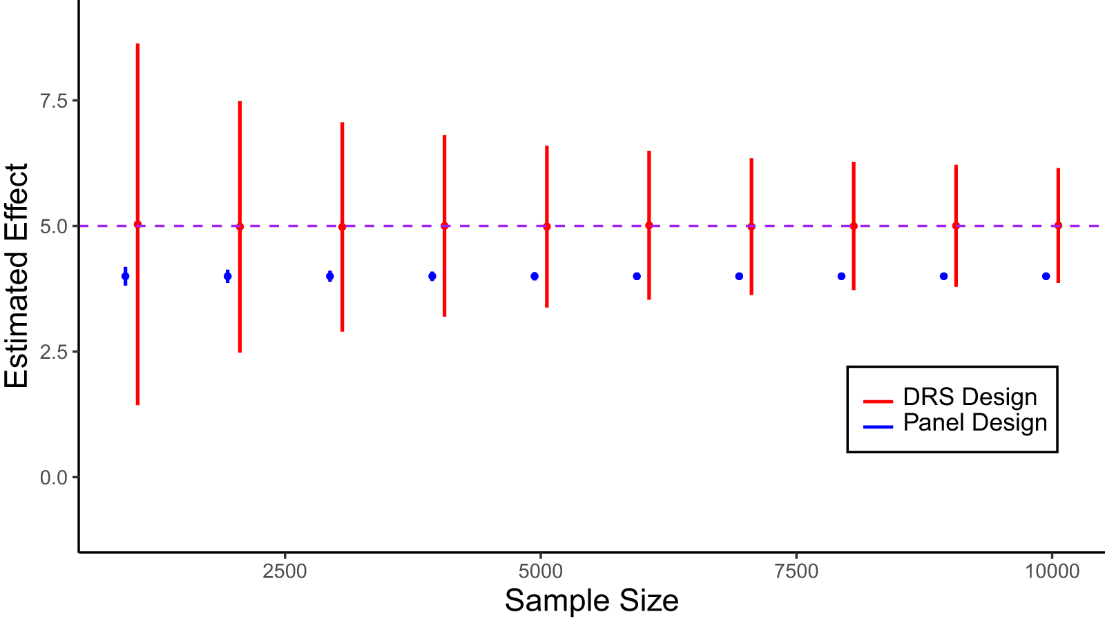
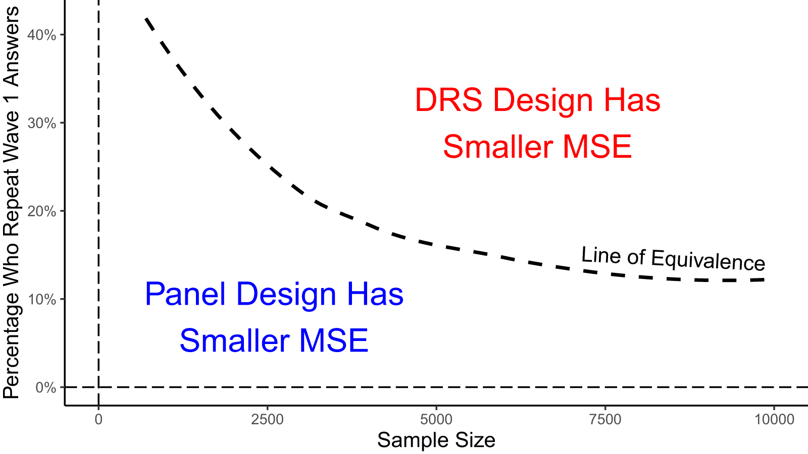


 Open access