2. Solvency II 1-Year Risk Horizon and the Economic Balance Sheet

There are three basic elements to the Solvency II directives issued by the European Commission (2010) in respect to Risk Capital:

• ∙ For the purpose of calculating the risk margin (RM) and understanding the hypothetical flow of capital, it is assumed that Risk Capital is raised at the beginning of each year and any unused capital is returned to the capital provider at the end of the year;

• ∙ the analyses are conditional on the first (next) calendar year being in distress (99.5%);

• ∙ at the end of the first year in distress, the balance sheet can be restored in such a way that the company has sufficient Technical Provisions (TPs) (equivalently the Fair Value of Liabilities) to continue business or to transfer the liabilities to another risk bearing entity.

The Cost of Capital approach is used to calculate the RM for non-hedgeable risks. The RM represents the premium paid to the notional risk capital providers for providing Risk Capital.

As an insurer must be able to withstand a 1 in 200 year loss and still have sufficient capital for risk to be fairly transferred to a third party (European Commission, 2007, 2009b), it follows that the Best Estimate of Liabilities (BEL) and RM, collectively known as the TP, are the cornerstone of the Solvency II 1-year risk horizon.

(1) $${\rm TP}\, {\equals}\, {\rm BEL}{\plus}{\rm RM}$$

The regulation includes provision to discount TP by the risk-free rate. However, for simplicity the risk-free rate (the present value discount) is omitted from all calculations in this paper.

3. SCR: A Naïve Definition

In order to demonstrate that the company has sufficient capital to sustain losses at the 99.5^th percentile in the first calendar year the effect of a 1 in 200 year loss in the next calendar year is to be estimated.

The BEL covers the loss up to the best estimate. Only the excess loss, the loss above the mean, is required as risk capital to sustain losses at the 99.5^th percentile.

Let Y denote a random variable representing the loss (the reserve).

In the reserving context, the Value-at-Risk (V@R) is the capital at risk for a quantile, α∈(0, 1), given the distribution of losses, Y, and the expected loss, $\bar{Y}$ .

(2) $$V\,@\,R_{\alpha } (Y)\, {\equals}\, F_{Y}^{{\, {\minus}\, 1}} (1\, {\minus}\, \alpha )\, {\minus}\, \bar{Y}$$

where F is the cumulative distribution function.

Consider a loss reserve distribution as displayed in Figure 1. The vertical bar displays the mean, 699M, of the distribution. The 75^th percentile of the distribution is 725M. The difference between the 75^th percentile and the mean, 27M (rounding), is the capital that would be lost if the mean reserve was booked and the losses actually came in at the 75^th percentile of the loss distribution. That is, the V@R is 27M. The probability of losing at least 27M is (1–α), which is 25%.

Figure 1

Value-at-risk at 75^th percentile for an example distribution.

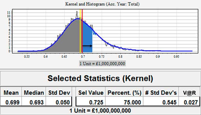
There are other measures of V@R such as Tail — V@R which calculates the average loss should the loss exceed the percentile, α. These alternatives are not considered in the Solvency II context, however they may be used in other solvency regulation (for instance, Swiss Solvency Test Swiss Federal Office of Private Insurance, 2004).

This simple definition of SCR is

(3) $$SCR^{1} \, {\equals}\, V\,@\,R_{{99.5\,\%\,}} (L_{1} )$$

where L ₁ is a random variable representing the first future calendar year loss and V@R _99.5% is the 99.5^th percentile of the V@R.

In this case, the Economic Balance Sheet for 1-year run-off is depicted in Figure 2.

Here, BEL ₁ is the BEL for year 1, that is

(4) $$BEL_{1} \, {\equals}\, E(L_{1} )$$

Figure 2

One-year run-off. TP, Technical Provision; SCR, Solvency II Capital Requirement

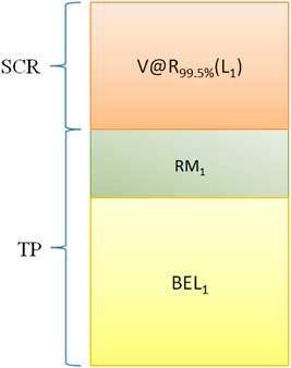
RM ₁ is the RM allocated for year 1, that is

(5) $$RM_{1} \, {\equals}\, s \cdot V\,@\,R_{{99.5\,\%\,}} (L_{1} )$$

where s is the spread — the return required above the risk free rate as specified in the regulation (European Commission, 2009a), and

(6) $$TP_{1} \, {\equals}\, BEL_{1} {\plus}RM_{1} $$

where TP ₁ is the TP (Fair Value) for year 1 (TP=TP ₁).

In the block diagram above, SCR is the Risk Capital raised from the (hypothetical) risk capital providers and RM ₁ is the cost to the insurer for access to this capital.

If the loss exceeds the BEL ₁ the Risk Capital (in this case SCR ¹) is drawn on. At the end of the year, the risk capital providers receive the SCR ¹ less the drawn capital.

RM ₁ is paid to the risk capital providers at the end of the year irrespective of the value of the loss.

4. SCR: Including Change in BEL

Incorporating calendar year correlation leads to an updated definition of SCR. If the first calendar year is in distress, the conditional loss distributions for subsequent years will have higher mean losses.

If the first year is in distress, the adjustments in the mean losses for subsequent years should be part of the Risk Capital raised. This way the BEL can be restored to Fair Value at the beginning of the second calendar year. The business can then continue to operate or the liabilities can be transferred to another risk bearing entity.

We denote the measure including these increments as SCR ². This definition is closely related to the definition of the CDR — see section 7. The change in the mean is equivalent to change in own funds when a distress event occurs.

That is

(7) $$SCR^{2} \, {\equals}\, SCR^{1} {\plus}\mathop{\sum}\limits_{i\, {\equals}\, 2}^n \Delta BEL_{i} $$

where

(8) $$\Delta BEL_{i} \, {\equals}\, BEL_{i} \mid(L_{1} \, {\equals}\, \lambda )\, {\minus}\, BEL_{i} $$

BEL _i denotes E(L _i ), and BELi|(L ₁=λ) is the mean of the conditional distribution of L _i (loss in calendar year i) given that the first year is in distress, that is (L ₁=λ), where

(9) $$\lambda \, {\equals}\, E(L_{1} ){\plus}V\,@\,R_{{99.5\,\%\,}} (L_{1} )$$

and n is the number of future calendar years in the calendar year liability stream.

The 2 years in run-off case is illustrated in Figure 3. The event that L ₁=λ is designated by ξ.

Figure 3

Two-year run-off. TP, Technical Provision; SCR, Solvency II Capital Requirement

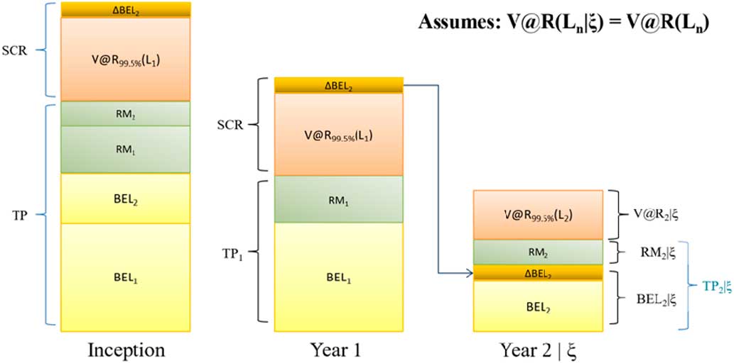
Consider the block diagram in Figure 3.

Given year 1 is in distress, we study year two first.

For the conditional distribution L ₂|ξ the increment in mean (above the unconditional distribution of L ₂) is ΔBEL ₂.

The event ξ results in (1) drawing on the risk capital for year 1 and (2) re-estimation of BEL at year 2 and hence SCR ² is the sum of the V@R plus the ΔBEL ₂.

The RM, RM ₁, is now based on an SCR that includes ΔBEL ₂.

The balance sheet at inception contains the sum of the BELs, the sum of the RMs, and the SCR ².

The flow of capital should the first year be in distress is as follows:

• ∙ BEL ₁ and V@R _99.5%(L ₁) are consumed;

• ∙ BEL ₂+ΔBEL ₂ is allocated to year 2 to restore the mean loss to conditional mean;

• ∙ RM ₂ is allocated to the RM for year 2;

• ∙ RM ₁ is returned to the risk capital provider;

• ∙ RM ₂ is left unchanged.

However, should the first year be in distress, it is likely that the V@R _99.5%(L ₂|ξ) will be larger than V@R _99.5%(L ₂). Let ΔRM ₂ be the difference between the RM RM ₂ and the RM RM ₂|ξ. Additional capital is needed to restore the Economic Balance Sheet to its Fair Value. This is necessary to satisfy the Solvency II objective that the liability risk can be fairly transferred to a third party (European Commission, 2007, 2009b).

SCR ² acknowledges the need for recalculation of future years after a distress year but fails to carry it through to every component of the TP. This leads to SCR ³.

5. SCR: Including Change in TP

Figure 4 includes the increment in RM in year 2 assuming the first year is in distress.

Figure 4

Two-year run-off including ΔTP. TP, Technical Provision; SCR, Solvency II Capital Requirement

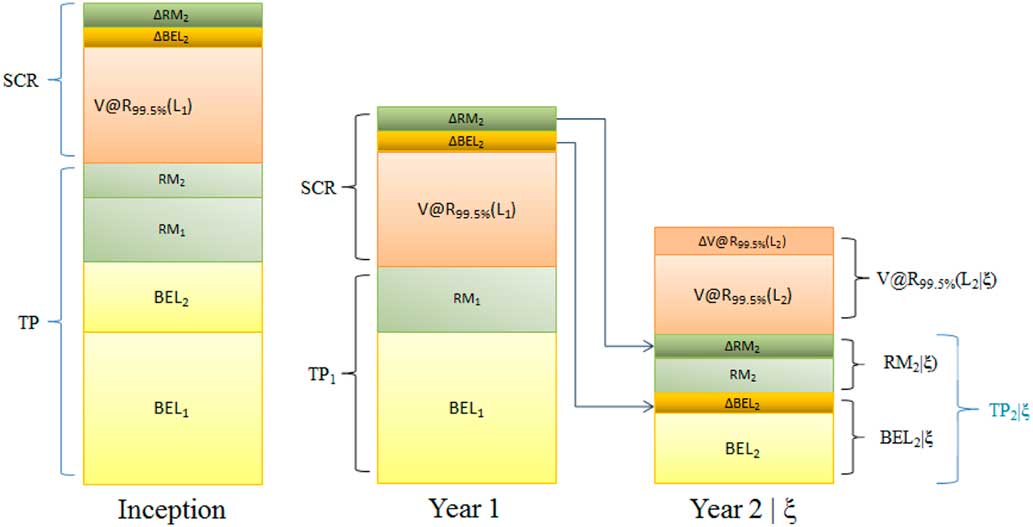
Given year 1 is in distress, the increase in V@R _99.5%(L ₂) is denoted by ΔV@R _99.5%(L ₂). This leads to an increase in the RM for year 2, ΔRM ₂. The ΔRM ₂ and ΔBEL ₂ are both incorporated in the SCR for year 1 allowing the Economic Balance Sheet to be fully restored to its Fair Value at the beginning of year 2 in the event of distress. The cost of capital for holding SCR, RM ₁, is adjusted to include the cost of also holding ΔRM ₂ and ΔBEL ₂.

The flow of capital should the first year be in distress is as follows:

• BEL ₁ and V@R _99.5%(L ₁) are consumed;

• BEL ₂+ΔBEL ₂ is allocated to year two to restore the mean loss to conditional mean;

• RM ₂+ΔRM ₂ is allocated to the RM for year 2;

• RM ₁ is returned to the risk capital provider.

At inception the two Δ’s are part of the risk capital in year 1 but they are allocated to the TP in year 2 in the distress event.

The definition of SCR ³ can be appropriately extended to a multiple year run-off as follows:

(10) $$SCR^{3} \, {\equals}\, SCR^{2} {\plus}\mathop{\sum}\limits_{i\, {\equals}\, 2}^n \Delta RM_{i} $$

If spread is 0%, then SCR ³=SCR ². However, the Economic Balance Sheet would then be different as the TP is different.

6. Variation in the Mean Ultimate Loss 1 Year Hence and the Claims Development Result

Let’s decompose the ultimate loss, L _Ult , as the sum of the first future year calendar year loss and the sum of subsequent calendar year losses:

(11) $$L_{{Ult}} \, {\equals}\, L_{1} {\plus}\Sigma _{{i\, {\equals}\, 2}}^{n} L_{i} $$

Then the expectation of ultimate loss conditional on the first future year loss E(L _Ult |L ₁) is

(12) $$E(L_{{Ult}} \! \mid \! L_{1} )\, {\equals}\, L_{1} {\plus}\Sigma _{{i\, {\equals}\, 2}}^{n} E(L_{i} \! \mid\! L_{1} )$$

The quantity

(13) $$\Delta _{1} L_{{Ult}} \, {\equals}\, E(L_{{Ult}} \!\mid\!L_{1} )\, {\minus}\, E(L_{{Ult}} )$$

is a random variable dependent on L ₁ that represents the variation in the mean ultimate loss. We denote it by VMU(L ₁) or simply VMU. In the Solvency II literature, −Δ₁ L _Ult is commonly referred to as the CDR (Merz & Wüthrich, Reference Merz and Wüthrich2008; England, Reference England2011). The VMU, is a more informative descriptor and under a distress scenario it is positive. (See discussion.)

The expected value of the VMU is 0. That is

(14) $$E(\Delta _{1} L_{{Ult}} )\, {\equals}\, E(E(L_{{Ult}} \!\mid\!L_{1} ))\, {\minus}\, E(L_{{Ult}} )\, {\equals}\, 0$$

Taking the variance of the VMU produces the following:

(15) $$Var(VMU)\, {\equals}\, Var(E(L_{{Ult}} \!\mid\!L_{1} ))$$

which is the same as the variance of the CDR.

This quantity represents the variance of the conditional mean ultimate 1 year hence.

This metric is important for senior management as it contextualises year to year changes in the estimate of mean ultimate. For a model and forecast scenario that are consistent there is statistical variation in the mean ultimate 1 year hence. That is, when a model and forecast scenario are updated with 1 year of new data, forecast scenario assumptions remaining consistent, variation in the mean ultimate is expected. See the example in section 8.

Indeed, by the law of total variance, Var(L _Ult ) can be decomposed as follows:

(16) $$Var(L_{{Ult}} )\, {\equals}\, E(Var(L_{{Ult}} \!\mid\!L_{1} )){\plus}Var(E(L_{{Ult}} \!\mid\!L_{1} ))$$

The variance of the ultimate is decomposed into two parts. E(Var(L|L ₁)) and the change in the mean ultimate, Var(E(L|L ₁)). Substituting using equation 15 gives:

(17) $$Var(L_{{Ult}} )\, {\equals}\, E(Var(L_{{Ult}} \!\mid\!L_{1} )){\plus}Var(VMU)$$

(18) $$Var(VMU)\, {\equals}\, E(Var(L_{{Ult}} )\, {\minus}\, Var(L_{{Ult}} \!\mid\!L_{1} ))$$

The information acquired when the next year’s results are known will reduce the variance of the ultimate. The variation contributed by the first future calendar year is removed (the losses are known), the subsequent parameter uncertainty is lower, and the forecast horizon is shorter. The mean reduction is: E(Var(L _Ult )–Var(L _Ult |L ₁)). By (18) this is the Variance of the VMU.

The proportion of the VMU component is indicative of the sensitivity to the next calendar year’s losses. If Var(VMU) takes a large proportion of the total variance, then the expected ultimate is very sensitive to the losses in the next year. Conversely, if Var(VMU) takes a low proportion of the total variance then the effects of re-parameterisation after year 1 are swamped by the process volatility. The impact of correlations on the VMU are discussed in section 9.

7. The Relationship Between the VMU and SCR ²

In this section, we show that VMU(L ₁=λ)=SCR ². Where:

(19) $$\hskip -50pt\lambda \, {\equals}\, E(L_{1} ){\plus}V\,@\,R_{{99.5\,\%\,}} (L_{1} )$$

Now:

(20) $$\hskip -80pt VMU\, {\equals}\, E(L_{{Ult}} \! \mid\! L_{1} )\, {\minus}\, E(L_{{Ult}} )$$

(21) $$\qquad {\equals}\, L_{1} {\plus}\mathop{\sum}\limits_{i\, {\equals}\, 2}^n E(L_{i} \! \mid\! L_{1} )\, {\minus}\, E(L_{1} )\, {\minus}\, \mathop{\sum}\limits_{i\, {\equals}\, 2}^n E(L_{i} )$$

(22) $$\ \, {\equals}\, L_{1} \, {\minus}\, E(L_{1} ){\plus}\mathop{\sum}\limits_{i\, {\equals}\, 2}^n [E(L_{i} \! \mid\! L_{1} )\, {\minus}\, E(L_{i} )]$$

Consider VMU when L ₁ is in distress. We can then write:

(23) $$VMU(L_{1} \, {\equals}\, \lambda )\, {\equals}\, V\,@\,R_{{99.5\%\,}} (L_{1} ){\plus}\mathop{\sum}\limits_{i\, {\equals}\, 2}^n [E(L_{i} \! \mid\! L_{1} \, {\equals}\, \lambda )\, {\minus}\, E(L_{i} )]$$

(24) $$\, {\equals}\, V\,@\,R_{{99.5\%\,}} (L_{1} ){\plus}\mathop{\sum}\limits_{i\, {\equals}\, 2}^n \Delta BEL_{i} $$

Given that calendar year loss correlations are positive, the ΔBEL _i are typically positive:

(25) $$VMU(L_{1} \, {\equals}\, \lambda )\, {\equals}\, \, {\minus}CDR(L_{1} \, {\equals}\, \lambda )\, {\equals}\, SCR^{2} $$

In the standard formula, one method to calculate the SCR is to calculate the V@R _99.5%(VMU).

Calculating the 99.5^th percentile of VMU is not equivalent to the realisation of VMU(L ₁=λ).

8. The Distribution of VMU (-CDR)

In order to find the theoretical distribution of VMU it is necessary to have loss distributions projected by calendar year and their correlations because the measure is inherently linked with calendar time.

The distributions going forward will depend on the future process volatility, the parameter estimates and their associated uncertainties. Correlations between the calendar year loss distributions are driven by parameter uncertainty. The magnitude of the correlations will also depend on process volatility.

The distribution of VMU is the sum of the conditional means (conditional on the first calendar year) minus the unconditional means: $$\Sigma _{{i\, {\equals}\, 2}}^{n} (E(L_{i} \!\mid\!L_{1} )\, {\minus}\, E(L_{i} ))$$ .

The unconditional means, E(L _i ), are the mean losses based on the original model. In order to estimate the distribution of VMU, the following steps apply:

1. 1. Use the model to simulate the next calendar year (L ₁).

2. 2. Re-estimate the same model, including the data for L ₁, to obtain conditional means (E(L _i |L ₁):i>1).

For the first calendar year, the difference between the simulated values and the unconditional mean of this year is (L ₁–E(L ₁)). For subsequent years, i=2 to n, the ith difference between the conditional means and the unconditional means is (E(L _i |L ₁)−E(L _i )).

The sums of these differences are realisations of VMU.

To illustrate, assume a model specifies the loss distributions by calendar year as in Table 1. The total mean outstanding is 7, 138, 147 total losses paid to date of 10, 221, 194. The corresponding mean ultimate is 17, 138, 147.

Table 1

Example future calendar year distributions.

If we simulate the next calendar year using the model, the distribution of the simulations for that year will have a mean of 1, 864, 457 and a SD of 75, 213. For each simulation, the model parameters are updated and used to obtain mean projections of the years E(L _i |L₁) where i>1.

This leads to a distribution for the VMU, $$\Sigma _{{i\, {\equals}\, 2}}^{n} (E(L_{i} \! \mid\!L_{1} )\, {\minus}\, E(L_{i} ))$$ . One such simulation is shown in Figure 5.

Figure 5

Distribution of Variation in Mean Ultimate

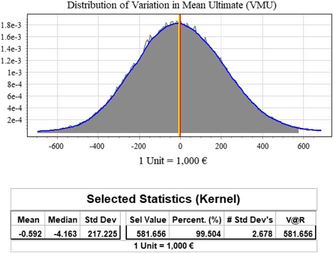
The 99.5^th percentile of the VMU, 581, 656, is highlighted. The distribution of the VMU shows that there is a 1 in 200 probability the current estimate of the mean ultimate, 17, 138, 147, will be increased by at least 581, 656, after next year’s losses are realised. See section 10 for the relationship between the VMU at the 99.5^th percentile and SCR ².

9. Decomposing the Total Variation of L _Ult into L ₁ and L _{2 …} L _n Given L ₁

Consider two hypothetical cases where we assess the value of information about the next calendar year’s losses. This is discussed in the context of the VMU.

High correlations imply a lot of value in knowing the next calendar year’s loss. Low correlations imply knowledge of the next calendar year does not result in knowledge about future calendar years.

(26) $$Var(E[L_{{Ult}} \! \mid\! L_{1} ])\, {\equals}\, Var(L_{1} {\plus}\mathop{\sum}\limits_{i\, {\equals}\, 2}^n E(L_{i} \,\mid\,L_{1} ))$$

9.1. Case 1: Low Correlation Between Future Calendar Years

Assume there is very little correlation in the calendar year loss distributions (Table 2).

Table 2

Case 1: low future calendar year correlations

Since the correlation between L _i and L ₁ is close to 0 (Table 2), then E(L _i |L ₁) ≈ E(L _i ). It therefore follows that:

(27) $$Var(E[L_{{ULt}} \! \mid \! L_{1} ])\,\approx\,Var(L_{1} )$$

The forecast table with means, standard deviations, and expected variation conditional on the next calendar year’s data are shown in Table 3.

In Table 3, the variation in the next calendar year’s loss, 796, 830, is close to the total variation in the expected ultimate, conditional on the next calendar year’s data, 807, 822.

Table 3

Case 1: forecast table and contribution to variation in mean ultimate (VMU)

When the correlation between calendar years is close to 0, the variance of the sum of the conditional expectations, $$Var(\mathop{\sum}\nolimits_{(i\, {\equals}\, 2)}^n E(L_{i} \! \mid\! L_{1} ))$$ , is close to 0.

The contribution of the variation in the mean losses, L ₂ … L _n conditional on L ₁, to the VMU is negligible compared to the variation in L ₁ (Table 3).

9.2. Case 2: High Correlation Between Future Calendar Years

Consider high positive correlation between calendar year loss distributions (Table 4).

Table 4

Case 2: high future calendar year correlations

The importance of the covariance terms as contributors to the total variation increases as the correlation increases.

(28) $$Var(E[L\!\mid\!L_{1} ])\, {\equals}\, Var(L_{1} {\plus}\mathop{\sum}\limits_{i\, {\equals}\, 2}^n E(L_{i} \,\mid\,L_{1} ))$$

(29) $$\, {\equals}\, Var(L_{1} ){\plus}2 \cdot cov(L_{1} ,\mathop{\sum}\limits_{i\, {\equals}\, 2}^n E(L_{i} \!\mid\!L_{1} )){\plus}Var(\mathop{\sum}\limits_{i\, {\equals}\, 2}^n E(L_{i} \!\mid\!L_{1} ))$$

In this case, the contribution of $$2 \cdot cov(L_{1} ,\mathop{\sum}\nolimits_{i\, {\equals}\, 2}^n E(L_{i} \!\mid\!L_{1} ))$$ and $$Var(\mathop{\sum}\nolimits_{i\, {\equals}\, 2}^n E(L_{i} \!\mid\!L_{1} ))$$ dominate the contribution of Var(L ₁) (Table 5) to the VMU.

Table 5

Case 2: forecast table and contribution to variation in mean ultimate (VMU)

In Table 5, the variation in the next calendar year’s loss, 110, 997, is a small fraction of the total variation in the expected ultimate conditional on the next calendar year’s data, 1, 308, 787. Taking into consideration the correlation between the distributions, the losses in L ₁ contribute to about 15% of the variation in the VMU compared to 99.99% of the variation in Case 1.

10. VMU _99.5% Versus SCR ²

The 99.5^th percentile of the VMU is usually not the same as the value of SCR ². These measures will only be similar if the correlations between future calendar year loss distributions approach 1 (see section 9.2).

If the correlations between future calendar years are close to one, then:

(30) $$SCR^{2} \,\approx\,VMU_{{99.5}} $$

SCR ² and VMU _99.5 are approximately the same.

When the correlations are high, looking at the percentile (99.5) of the sum of the changes is close to taking the sum of the 99.5^th percentiles for each year. That is, it is closer to taking the V@R _99.5 of L _Ult .

If there is no parameter uncertainty then the correlation between calendar periods is 0. That is, E[L _i |L ₁]=E[L _i ] and:

(31) $$SCR^{2} \,\lt\,\!\lt\,VMU_{{99.5}} $$

In the case of SCR ², only the first year is in distress and subsequent ΔBELs are not likely to be at the same percentile at the same time.

11. Solvency II Standard Formula and SCR

In the Solvency II context, the QIS5 SCR standard formula is based on E(L) and Var(CDR) (=Var(VMU)) (European Commission, 2010).

The V@R _99.5%(VMU) is one of the approximations for SCR based on the standard formula (European Commission, 2010). We denote this SCR as SCR ⁴. Since the distress in the next calendar year is not explicitly calculated, it is effectively assumed that V@R _99.5%(VMU) corresponds to being in distress in the first year and having sufficient capital to restore the means of the Economic Balance Sheet (RMs are ignored).

However, the recommended approach in the standard formula is to fit a log-normal to the mean (Provision of Claims Outstanding=E(L)) and Variance (Var(CDR)). The log-normal distribution is not necessarily a good proxy for the distribution of VMU. (See QIS5 technical specifications European Commission (2010), paragraph SCR.9.18.) This approximation to SCR ⁴ we denote SCR ⁴*.

SCR ⁴* is not related to SCR ¹, SCR ², SCR ³ nor even to the distribution of VMU and therefore to SCR ⁴. The differences between SCR ⁴ and any of the other SCR calculations are model dependent (and data dependent).

Consider the two cases from section 9. In the situation where future calendar year correlations are close to 0 (Case 1), SCR ¹, SCR ², SCR ³, and SCR ⁴ are about the same (Table 6) — they are within expected statistical variation. The lognormal distribution approximation, SCR ⁴*, produces a much lower estimate — in fact lower than the 99.5^th percentile of the first calendar year (SCR ¹). The company would not even be able to pay for the losses up to the 99.5^th percentile even if the model was completely correct.

Table 6

SCR comparison for Cases 1 and 2

However, when the parameter uncertainty and correlations between the loss distributions by calendar year are high (Case 2), SCR ⁴* well exceeds SCR ⁴>SCR ²>SCR ³>>SCR ¹ (Table 6).

Note that in the second example, SCR ²>SCR ³ as the V@R _99.5 requirements decrease, even in the case of distress, as improved knowledge of the parameter actually reduces the V@R in subsequent calendar years. The calculation of SCR ³ takes advantage of this knowledge whereas SCR ² is oblivious.

12. Summary

Four methods of estimating the appropriate SCR were compared along with an approximation. The calculation method most consistent with the Solvency II directives is the SCR ³ estimate as presented in Munroe et al. (Reference Munroe, Odell, Sandler and Zehnwirth2015). This calculation is consistent with the Solvency II directives and also ties in with the way one would calculate RMs.

The simpler calculations, SCR ¹ and SCR ², usually do not provide sufficient capital to restore the Economic Balance Sheet should a distress event occur. Estimation of required risk capital is reasonable only in very particular conditions.

All measures of SCR in Table 7 assume the model used to estimate the loss distributions is correct.

Table 7

Solvency II Capital Requirement (SCR) comparison for Cases 1 and 2

The standard formula calculation for SCR based on the distribution of the VMU, SCR ⁴, is too conservative when correlations are high. The approximation to the distribution of VMU using a lognormal distribution assumption to E(L) and Var(VMU) was shown to be too conservative (section 11) when correlations were high, and far too optimistic when correlations were low. The lognormal distribution approximation for SCR ⁴, SCR ^4*, is a very poor estimator of SCR ⁴.