


1. Introduction
The massive international reserve accumulation of Emerging Market Economies (EMEs) from the late 1990s has provoked active discussion on its motivation. There are widely accepted explanations in the literature: The precautionary view argues that reserves are accumulated as a buffer against sudden stops, and the mercantilist view considers reserves as byproducts of the intervention policy that promotes export competitiveness. However, EME policymakers have more often argued that they had to accumulate reserves to counter excessive capital inflows.Footnote 1 According to them, large capital inflows cause many problems, such as credit expansion and asset price inflation, and reserve accumulation is inevitable to maintain macroeconomic stability.
In this study, we present empirical evidence and a theoretical model of reserve accumulation that corroborate the arguments of EME policymakers. Our analysis is based on three observations about reserve accumulation and capital flows in EMEs. First, gross capital inflows (foreign investors’ purchases of EME assets) are positively correlated with reserve accumulation. This relationship is illustrated in Panel (a) of Figure 1 (gray dots), which presents a scatter plot of gross capital inflows against reserve accumulation across sample EMEs. The positive correlation between gross inflows and reserve outflows is in line with the well-known fact in the literature that international reserve holdings are positively correlated with external liabilities (e.g. Alfaro and Kanczuk, Reference Alfaro and Kanczuk2009). The second observation, which has not been extensively documented or analyzed in prior research, is the positive association between direct investment inflows and reserve outflows. This relationship is also illustrated in Panel (a) with red squares.Footnote 2 The final observation is that reserve accumulation is more active when the country has more restrictions on gross capital outflows (domestic investors’ purchases of foreign assets). Panel (b) of Figure 1 provides suggestive evidence that the magnitude of reserve accumulation per gross direct inflow is greater in countries with more restrictions on capital outflows (red circles).
Capital inflows and reserve accumulation.Notes: This figure shows the relationship between reserve flows and gross capital inflows for the sample of empirical analysis in this study: 34 EMEs over the 1999–2019 period in quarterly frequency. Panel (a) shows each country’s average total gross capital inflows and direct inflows against reserve accumulation. Panel (b) shows each country’s average gross direct inflows and reserve accumulation over the same period. Countries with the above-median Overall Outflow Restrictions Index (kao) of Fernández et al. (Reference Fernández, Klein, Rebucci, Schindler and Uribe2016) are plotted with red circles. Two countries are omitted from the figure to enhance visibility (Ecuador and Iceland). All the data are sourced from the IMF International Financial Statistics.

Based on these observations, we formulate a new theory that views reserve accumulation as an optimal response to large capital inflows. A sudden surge in direct investment (FDI) inflows to EMEs causes imbalances in the current account. If there is no friction, corresponding gross capital outflows should occur from the private sector (Ricardian equivalence). However, in EMEs, the private sector cannot invest abroad sufficiently due to various frictions such as financial repression (legal restrictions)Footnote 3 and underdevelopment of financial institutions (lack of knowledge and skills regarding overseas investment). As the country needs to make capital outflows to restore macroeconomic balance (i.e., to smooth consumption over time), the public sector may instead invest abroad in the form of international reserves.
While it is common in the literature and policy discussions to associate capital flow surges primarily with portfolio and banking inflows, there is empirical evidence that surges are more prevalent with FDI flows and that FDI inflows are also affected by global factors. Forbes and Warnock (Reference Forbes and Warnock2021) document that, over the period 1985–2020, 17.6% of EMEs experienced surges in FDI—by their rigorous definition—surpassing the frequency of surges in portfolio debt (11.4%), equity (12.0%), or banking (11.0%) flows. Furthermore, Albuquerque et al. (Reference Albuquerque, Loayza and Servén2005) show that global factors play a significant role in driving FDI flows. They show that FDI flows are sensitive to variables related to global investors’ discount factors and opportunity cost of capital. Based on these findings, our analysis treats FDI as responsive to shifts in global financial conditions.
We begin our analysis by establishing empirical findings from EME panel data. We aim to understand whether EMEs build reserves in response to exogenous capital inflows. If that is the case, we want to know which countries are more active in those responses and, finally, what asset types of capital inflows they are sensitive to. We examine these three questions based on panel data of 34 EMEs over 20 years from 1999 to 2019. We investigate the differences among countries with varying levels of external investment capacity and different types of capital inflows. Specifically, we assess financial frictions that hinder external investment in two dimensions: government restrictions and underdeveloped financial institutions. We confirm a positive association between gross capital inflows, particularly direct investment inflows, and reserve accumulation. The relationship is more pronounced in countries with a higher level of financial friction. In addition, we apply a two-stage regression approach to represent exogenous capital inflows. In the first stage, we estimate push factor-driven capital inflows by projecting each country’s capital inflows onto the global push factors of capital flows. In the second stage, we examine the reserve responses to these estimated inflows. We find that the initial results hold true even when considering push factor-driven capital inflows.
We provide a theoretical model for reserve accumulation in this context. It is a three-period model of Fisherian deflation (à la Bianchi, Reference Bianchi2011; Korinek, Reference Korinek2018; Jeanne and Korinek, Reference Jeanne and Korinek2019). We add two ingredients to the existing model: 1) frictions on capital outflows and 2) global push factor-driven capital inflows in the form of direct investment. First, we assume that poor financial development hinders residents’ investment abroad. This assumption on private outflows creates a type of imperfect capital mobility akin to Fanelli and Straub (Reference Fanelli and Straub2021), but specifically for capital outflows. Second, we assume that a global investor purchases the country’s capital (direct investment). This captures large direct investment inflows to an EME, driven by global push factors. As the investor pays for the capital, EME residents earn a large current income while they lose claims to future output generated by the sold-out capital. These model setups are designed to rationalize our empirical findings.
Our parsimonious model explains why EMEs facing large capital inflows have incentives to accumulate reserves. In this model, direct investment inflows make the EMEs less prone to sudden stops represented by an occasionally binding borrowing constraint in the second period. However, beyond a certain level, direct investment inflows necessitate savings abroad for consumption smoothing over time. This is because larger direct investments result in a greater portion of future output being allocated to foreign investors. A problem occurs when the private sector cannot make sufficient investments abroad and when the investments are socially inefficient due to friction. In this scenario, significant capital inflows lead to appreciation of the domestic currency and consumption booms. Therefore, the government is incentivized to accumulate reserves to generate capital outflows and help smooth household consumption. In our model, reserve accumulation supplements the private sector’s insufficient capital outflows and replaces the socially inefficient private outflows.
The mechanism by which reserve accumulation proves to be effective in this paper fundamentally differs from previous studies. Existing studies assume constraints on foreign borrowing or frictions on capital inflows to make reserve accumulation effective (See, for example, Gabaix and Maggiori, Reference Gabaix and Maggiori2015; Arce et al. Reference Arce, Bengui and Bianchi2019; Fanelli and Straub, Reference Fanelli and Straub2021). In contrast, the effectiveness of reserve accumulation in our model arises from frictions on capital outflow. As marginal inefficiencies or social costs of private outflows are proportional to the size of the outflows, reserve accumulation becomes an efficient policy tool when the EME faces excessive capital inflows. Furthermore, in this study, the role of reserve accumulation is not entirely replaceable by capital controls, contrasting with previous studies like Davis et al. (Reference Davis, Fujiwara, Huang and Wang2021). In fact, we formally show that the optimal policy in response to excessive direct investment inflows is to accumulate reserves while taxing private capital outflows, which is consistent with our empirical findings.
Our model, combined with empirical findings, helps us to understand the rapid increases in reserve holdings of EMEs beginning from the late 1990s. After opening up the financial accounts in the 1990s, many EMEs had to deal with surges in gross capital inflows, particularly in the form of FDI. We explain why some countries hoard more reserves than others. In countries with underdeveloped financial sectors or financial repression, the role of the official sector in stabilizing net flows is greater. Additionally, our model provides important implications for the debate on currency manipulation: Do EMEs depreciate their currencies to boost their exports? We argue that the size of reserves is not a good litmus test for exchange rate manipulation. As discussed above, reserve accumulation might be a passive reaction to the excessive capital inflows caused by global push factors.
Related literature This study is related to several strands of literature in international macroeconomics. First, our study belongs to the literature on why EMEs hold large foreign reserves. The existing literature broadly adheres to two different views: the mercantilist and precautionary viewpoints. The mercantilist view argues that foreign exchange reserves are byproducts of exchange rate policies aiming to boost exports via currency depreciation.Footnote 4 On the other hand, the precautionary view highlights the historical fact that most EMEs began building their reserves stocks after experiencing financial crises, in particular the East Asian crisis of 1997.Footnote 5 Studies in this group argue that EMEs accumulate reserves to protect themselves against sudden stops. The most recent works in this line of research include Jeanne and Sandri (Reference Jeanne and Sandri2023).Footnote 6 They introduce a model wherein EMEs accumulate and decumulate reserves to counter global financial cycle. We contribute to the literature by suggesting a different view on reserve accumulation by EMEs. In our theory, EMEs accumulate reserves to prevent consumption booms caused by capital inflows. This accumulation of reserves serves as an optimal form of savings in response to these inflows. The purpose of this saving is to transfer the income generated during capital inflow bonanzas to the future.
Our study also connects to prior studies that examine the positive relationships between FDI liabilities and reserve assets. This positive correlation is first documented by Dooley et al. (Reference Dooley, Folkerts-Landau and Garber2003). They argue that EMEs depreciate their currencies to attract direct investments to utilize otherwise wasteful resources in the economy, such as labor. Matsumoto (Reference Matsumoto2022) and Wang (Reference Wang2019) share similar ideas. They introduce a small open economy model in which EMEs accumulate reserves to attract more FDI. While these studies interpret the observed correlations based on the mercantilist view, we provide alternative explanations for the same fact. In our view, reserve accumulation is a response to direct investment inflows; capital inflows cause reserve accumulation. We provide evidence that reserve accumulation increases when direct investment inflows occur due to global push factors, and this finding cannot be explained by existing models.Footnote 7
Finally, this study adds to the existing literature on the effectiveness of FX market interventions under imperfect capital mobility. Gabaix and Maggiori (Reference Gabaix and Maggiori2015) show how the limitations in arbitrage capacity within global asset markets explain important puzzles in the exchange rate literature. Fanelli and Straub (Reference Fanelli and Straub2021) derive the general principles of FX market interventions from a slightly different micro-foundation. Davis et al. (Reference Davis, Devereux and Yu2023) incorporate the imperfect capital mobility of Gabaix and Maggiori (Reference Gabaix and Maggiori2015) into a sudden stop model to study the role of the FX market intervention in preventing sudden stops. In modeling frictions in international capital flows, we mainly follow Fanelli and Straub (Reference Fanelli and Straub2021); however, we extend their modeling technique to EMEs’ private capital outflows. Our new insight is that EME policy authorities intervene not only to manage spreads on borrowing rates but also to respond to excessive capital inflows. Our study is similar to Davis et al. (Reference Davis, Devereux and Yu2023) as we incorporate the idea of imperfect capital mobility into a sudden stop model. However, our study stands apart by offering distinct contributions. While Davis et al. (Reference Davis, Devereux and Yu2023) focus on economies where private agents borrow abroad and face a sudden stop triggered by rising global interest rates, our model considers the opposite case in which the private sector saves abroad. In our environment, reserve holding generates benefit even in the absence of a sudden stop.Footnote 8
Layout The subsequent sections of this paper are structured as follows. Section 2 conducts a formal exploration of empirical regularities that serve as the foundation for our model. Section 3 introduces the novel model that provides new insights into reserve accumulation. Finally, in Section 4, we conclude and discuss the implications of the findings.
2. Empirical analysis
This section examines the empirical observations that underpin our theory. Our goal is to investigate whether EMEs indeed amass reserves in response to gross capital inflows, as they claim. In addition, we seek to identify the types of countries that are more inclined to exhibit such responses and specify the types of capital inflows to which they are particularly sensitive. To achieve this, we analyze a panel of EMEs and explore the relationship between gross capital inflows and reserve accumulation. We compare countries with varying levels of friction that deter residents from making overseas investments and analyze various types of asset flows. In addition, we employ two-stage regressions. In the first stage, we extract the exogenous component of gross capital inflows using the global push factors of capital flows. Then, we examine how EMEs respond to these exogenous parts of inflows with reserve accumulation.
2.1. Data and sample
The main data for the analysis are sourced from the IMF International Financial Statistics (IFS). We obtain quarterly capital flows documented in the official balance-of-payment statistics from the IFS. Reserve accumulation was popularized after many EMEs opened their financial accounts in the 1990s. Hence, we choose the sample period 1999–2019.Footnote 9
The sample countries are not chosen arbitrarily. Starting from the full sample of countries in the IFS, we exclude advanced economies and Eurozone countries. Among the remainders, countries with less than 12 quarterly observations of regression variables are excluded. This is necessary because we perform two-step regressions, wherein the first step is a country-by-country time series regression. This sample definition provides us with a total of 34 countries.Footnote 10
Table 1 provides the summary statistics for our sample. We adjust the nominal value with the US CPI to measure it in the 2010 US dollar value. Reserve accumulation is our dependent variable. The data is obtained from the balance-of-payment statistics; hence, they contain only the transaction component of the international reserve fluctuations. The mean reserve-accumulation-to-GDP ratio recorded in our sample was 0.51% per quarter, showing significant variation across different countries and time periods (standard deviation: 1.68).
Descriptive statistics

Notes: This table presents the descriptive statistics for the variables included in the regressions. The sample period is from 1999q1 to 2019q4. A total of 34 emerging economies are included in the sample. See footnote 10 for the full list of countries. Reserve accumulation and other capital flow data are obtained from the IMF International Financial Statistics. Gross capital outflow openness is calculated based on Fernández et al. (Reference Fernández, Klein, Rebucci, Schindler and Uribe2016). It is defined as “1-average of indicators for capital controls on residents’ capital flows.”.
For a shock that induces reserve accumulation, we consider gross capital inflows (non-resident investors’ acquisition of EME assets). We analyze different asset types of gross inflows: direct, equity, bond, and other (banking) investment flows. We normalize the variable using GDP by dividing quarter $t$
capital inflows by the sum of the quarters
$t$
capital inflows by the sum of the quarters $t-1$
to
$t-1$
to $t-4$
GDP. Descriptive statistics show that our sample countries experienced moderate capital inflows during the sample period. An average country received capital inflows amounting to 1.9% of its GDP every quarter. More than half of the inflows were in the form of direct investment (1.0% of the GDP).
$t-4$
GDP. Descriptive statistics show that our sample countries experienced moderate capital inflows during the sample period. An average country received capital inflows amounting to 1.9% of its GDP every quarter. More than half of the inflows were in the form of direct investment (1.0% of the GDP).
We investigate whether there are variations in reserve accumulation responses among countries with different levels of friction that impede residents’ ability to save abroad. We assess these frictions in two dimensions: government restrictions and the underdevelopment of financial institutions.
First, we examine restrictions on gross capital outflows. In many EMEs, financial repression hinders gross capital outflows. To expedite domestic capital accumulation and industrialization, EM governments often want to retain precious capital within their borders. As such, foreign exchange systems in many EMEs are devised to restrict capital outflows. Fernández et al. (Reference Fernández, Klein, Rebucci, Schindler and Uribe2016) note that there is a higher prevalence of outflow controls than of inflow controls, especially for middle- and low-income countries.
In order to assess this friction, we utilize the data on capital controls provided by Fernández et al. (Reference Fernández, Klein, Rebucci, Schindler and Uribe2016). They process the information in the IMF’s Annual Report on Exchange Rate Arrangements and Exchange Restrictions (AREAER) to derive qualitative indicators denoting the presence of capital controls for specific asset classes, distinguishing the residency of the buyer/seller. In our theory, the type of financial friction that necessitates reserve accumulation is that on gross capital outflows (capital flows by residents). Hence, we utilize their indicators on residents. By averaging all the indicators related to residents’ capital flows and subtracting the result from 1, we obtain the index “gross capital outflow openness” (GCO).Footnote 11 This index ranges from 0 to 1, with a value of 0 indicating the lowest level of openness in gross capital outflows, while a value of 1 signifies no restrictions on gross capital outflows. In our sample, the mean of GCO is 0.54, with a standard deviation of 0.39, enabling us to compare between countries with different levels of openness.
Secondly, we examine the underdevelopment of financial institutions. Developed financial institutions are essential for EME residents to invest abroad efficiently. We employ the index of financial institution development from the Global Financial Development Database (GFD) by Čihák et al. (Reference Čihák, Demirgüç-Kunt, Feyen and Levine2012). The GFD index on financial institutions assesses the level of financial institution development based on institutional size, accessibility, efficiency, and stability. This index (FII) also ranges from 0 to 1, with a higher value indicating a greater development. In our sample, the mean is 0.45 with standard deviation 0.17. Both GCO and FII indices are measured on an annual basis. To avoid simultaneity, we use the indices from the preceding year in our investigation of reserve accumulation.
2.2. Empirical strategy
We begin our empirical analysis with a simple two-way fixed effects model. Reserve accumulation is the regressand and gross capital inflows serve as the main regressor. To examine whether the reserve response is stronger for countries with more frictions on gross capital outflows, we interact the capital inflows with the gross capital outflow openness index (GCO) or the financial institution index (FII). This gives us the following specification:
 \begin{equation} \texttt {RA/GDP}_{i,t} = \delta _i + \delta _t + \gamma \; \texttt {K/GDP}_{i,t} + \theta \; \texttt {GCO}_{i,t-4} + \phi \; \texttt {GCO}_{i,t-4} \times \texttt {K/GDP}_{i,t} + \varepsilon _{i,t} \end{equation}
where $\delta _i$
and
$\delta _i$
and $\delta _t$
are country and quarter fixed effects, respectively. Both reserve accumulation (RA) and gross capital inflows (K) are normalized using GDP to make the results more comprehensible. Considering the potential correlation caused by GDP in both the regressand and regressor, we also examine reserve accumulation per capita as a robustness check. For the types of gross capital inflows, we examine the following categories: direct inflows, equity inflows, bond inflows, and other inflows (bank loans). We also consider total gross capital inflows, which include all these categories as well as financial derivatives inflows.
$\delta _t$
are country and quarter fixed effects, respectively. Both reserve accumulation (RA) and gross capital inflows (K) are normalized using GDP to make the results more comprehensible. Considering the potential correlation caused by GDP in both the regressand and regressor, we also examine reserve accumulation per capita as a robustness check. For the types of gross capital inflows, we examine the following categories: direct inflows, equity inflows, bond inflows, and other inflows (bank loans). We also consider total gross capital inflows, which include all these categories as well as financial derivatives inflows.
With the interaction term in Equation (1), we compare the reserve accumulation responses of countries with varying levels of friction. Our conjecture is that reserve accumulation would be more pronounced in countries with more frictions in residents’ investment abroad. In these countries, the private sector cannot channel funds abroad sufficiently in response to massive gross capital inflows, and thus have consumption booms which are not desirable from the social planner’s perspective. In this case, reserve accumulation can help smooth the consumption. Hence, we expect a larger accumulation of reserves for countries with more restrictions on gross capital outflows or with underdeveloped financial institutions. This corresponds to a positive $\gamma$
and a negative
$\gamma$
and a negative $\phi$
coefficient. The friction measures (GCO or FII) are lagged by one year relative to the capital flow variables. In the regression implementation, we winsorize the regressand and regressor to have reasonable value for their kurtosis (below 10). We cluster the standard error at the country level to adjust the error for possible auto-correlation within each country.
$\phi$
coefficient. The friction measures (GCO or FII) are lagged by one year relative to the capital flow variables. In the regression implementation, we winsorize the regressand and regressor to have reasonable value for their kurtosis (below 10). We cluster the standard error at the country level to adjust the error for possible auto-correlation within each country.
In further detail on our hypothesis, capital inflows are the cause, and reserve accumulation is the effect. While the effects can be analyzed by introducing exogenous capital inflows in a theoretical model, it is obviously difficult to address the endogeneity in empirical investigations. From the data, a positive association is expected between gross capital inflows and reserve accumulation. However, it could result from a reverse causality or a third factor affecting both. Reserve accumulation may also influence other private capital flows. Furthermore, many factors considered in international reserve management are correlated with capital flows.
We tackle the identification challenge by employing a two-stage regression method. Using global push factors of capital inflows, we isolate the exogenous parts of gross capital inflows to each country. As our sample consists of only small open economies, we can safely assume that the global push factors are exogenous to domestic fundamentals. For the push factors, we consider two variables: VIX and a US dollar index. The VIX reflects the risk appetites of international investors and is widely used as a representative indicator of the Global Financial Cycle in the literature (Rey, Reference Rey2015). The VIX is highly correlated with portfolio and banking flows. On the other hand, the exchange rate has important influences on direct investment flows and equity flows. Many studies report a close relationship between the exchange rate and FDI (e.g. Matsumoto, Reference Matsumoto2022). Thus, we use changes in the US dollar’s value as the second push factor. Specifically, we measure the value of the dollar using the Real Major Dollar Index (TWEXMPA) offered by the Federal Reserve. This index measures the US real effective exchange rate against major advanced economies (Euro Area, Canada, Japan, U.K., Switzerland, Australia, and Sweden). Notably, the US and these countries are not included in our sample. And we safely assume that the individual EM countries in our sample cannot influence this dollar index.
Specifically, in the first stage, we regress gross capital inflows on VIX and the US dollar index. We conduct the regression country-by-country and obtain the predicted capital inflow series for each country. The first stage regression equation is as follows:
 \begin{equation} \texttt {K/GDP} _{i,t} = \alpha _i + \beta _{1,i} \ln \texttt {VIX}_{t-1} + \beta _{2,i}\Delta \texttt {USD}_{t-1} + \gamma _i X_{i,t-4}+\varepsilon _{i,t}\quad \text{for each } i \end{equation}
where $X$
is the covariate (either GCO or FII), and is also included in the second stage regression, identical to Equation (1). The predicted value of regression (2) contains push factor-driven capital inflows. Note that estimating Equation (2) country-wise is the same as estimating the following single panel regression.
$X$
is the covariate (either GCO or FII), and is also included in the second stage regression, identical to Equation (1). The predicted value of regression (2) contains push factor-driven capital inflows. Note that estimating Equation (2) country-wise is the same as estimating the following single panel regression.
 \begin{equation} \texttt {K/GDP} _{i,t} = \sum _i \beta _{1,i} \;d_i + \sum _i \beta _{2,i} \;d_i \times \ln \texttt {VIX}_{t-1} + \sum _i \beta _{3,i} \;d_i \times \Delta \texttt {USD}_{t-1} + \sum _i \gamma _i d_i \times X_{i,t-4} +\varepsilon _{i,t} \end{equation}
where $d_i$
is a dummy variable for country
$d_i$
is a dummy variable for country $i$
. Therefore, we employ 102 instrumental variables: 34 country dummies and 68 interactions between those country dummies and the VIX and the dollar index. In the actual regression, we perform the above panel regression and obtain the F-statistics that are used to judge the fitness of the first stage. Then, for the second stage, we replace
$i$
. Therefore, we employ 102 instrumental variables: 34 country dummies and 68 interactions between those country dummies and the VIX and the dollar index. In the actual regression, we perform the above panel regression and obtain the F-statistics that are used to judge the fitness of the first stage. Then, for the second stage, we replace $\texttt {K/GDP}_{i,t}$
in regression (1) with the predicted capital inflow series (push factor-driven capital inflows). Because our regressor is a variable generated by regressions, we calculate the standard error using the bootstrapping method that encompasses both the first and the second stages.
$\texttt {K/GDP}_{i,t}$
in regression (1) with the predicted capital inflow series (push factor-driven capital inflows). Because our regressor is a variable generated by regressions, we calculate the standard error using the bootstrapping method that encompasses both the first and the second stages.
2.3. Results and interpretation
We first present the results of the total gross capital inflows, followed by a discussion of the different asset types of these inflows. See Table 2 for detailed results on total capital flows. Columns (1)–(3) show the standard ordinary least squares (OLS) regression result. As expected, reserve accumulation and gross capital inflows are strongly and positively correlated (Column 1). Furthermore, the positive correlation is stronger for countries with more limitations in residents’ investment abroad (low financial institution development in Column 2 and more restrictions on gross capital outflows in Column 3).
Baseline results on total gross capital inflows

Notes: The variable INDEX refers to either the Financial Institution Index (FII) or the Gross Capital Outflow Openness Index (GCO). They are lagged by one year. The sample period is from 1999q1 to 2019q4. The top and bottom 1% of the dependent variables and the top and bottom 3% of the capital flow variable are winsorized. Reported in brackets are the bootstrapped standard errors. Standard errors are clustered at the country level. *, * *, and * * * indicate statistical significance at the 10%, 5%, and 1% levels, respectively.
Starting from Column (4), we conduct the two-stage regression process: We first isolate the part of the capital inflows explained by the global push factors and then regress reserve accumulation on it. Since the first stage includes 34 regressions (country-by-country), we report only the F-statistics obtained from the combined regression (3) for the first stage. In Column (4) we find that the positive relationship between reserve and gross capital inflows arises from push factor-driven capital inflows and policy responses to it.
Columns (5) and (6) interact the predicted gross capital inflows with the financial institution index and the gross capital outflow openness measure, respectively. We find that reserve accumulation is positively associated with exogenous capital inflows (positive coefficients to K/GDP) but less so for countries with more developed financial institutions or higher levels of gross capital outflow openness (negative coefficients to the interaction terms). Numerically, the results indicate that when countries receive a 1% of GDP capital inflows driven by global factors, a country with the least developed financial institutions ( $\texttt {FII} = 0$
) or the strictest controls on capital outflows (
$\texttt {FII} = 0$
) or the strictest controls on capital outflows ( $\texttt {GCO}= 0$
) increases its reserves by 0.75% or 0.86% of GDP, respectively. In contrast, a country with the most developed financial institutions (
$\texttt {GCO}= 0$
) increases its reserves by 0.75% or 0.86% of GDP, respectively. In contrast, a country with the most developed financial institutions ( $\texttt {FII} = 1$
) or no capital outflow restrictions (
$\texttt {FII} = 1$
) or no capital outflow restrictions ( $\texttt {GCO} = 1$
) generally does not increase its reserves.
$\texttt {GCO} = 1$
) generally does not increase its reserves.
Column (7) does the same regression as in Column (6), but we normalize the reserve accumulation by population instead of GDP, transforming it into a per capita variable. We continue to normalize other capital inflow data using GDP. This approach is adopted to prevent the potential correlation that arises from normalizing both dependent and independent variables using GDP. The population is a relatively stable variable compared to GDP and is less endogenous to business cycles. Hence, many previous studies on economic growth and public debt utilize population normalization for either the dependent variable, the independent variable, or both. See Panizza and Presbitero (Reference Panizza and Presbitero2014) and Eberhardt and Presbitero (Reference Eberhardt and Presbitero2015). We find that our findings are robust to this change.
Next, in Table 3, we investigate different asset types of gross capital inflows. Columns (1)–(4) replicate the regression of Column (5) of Table 2 but examine direct, equity, bond, and other investment inflows, respectively. Likewise, Columns (5)–(8) reproduce the analysis of Column (6) from Table 2, but with different asset types of capital flows. Upon examining various types of gross capital inflows in relation to financial institution development (FII) in Columns (1)–(4), we observe that the coefficients for push factor-driven capital flows are positive, while those for the interaction between capital inflows and FII are negative across all regressions. However, statistical significance is achieved only for direct investment inflows and other inflows.
2SLS results on different types of flows

Notes: The variable INDEX refers to either the Financial Institution Index (FII) or the Gross Capital Outflow Openness Index (GCO). They are lagged by one year. The sample period is from 1999q1 to 2019q4. The top and bottom 1% of the dependent variables and the top and bottom 3% of the capital flow variables are winsorized. Standard errors are clustered at the country level. In Columns (5)–(10), they are obtained by the bootstrapping method. +, *, * *, and * * * indicate statistical significance at the 15%, 10%, 5%, and 1% levels, respectively.
The subsequent Columns (5)–(8) use gross capital outflow openness index (GCO). The baseline result from Column (6) in Table 2 remains robust across all capital flow types. To identify which inflow type most significantly triggers a reserve accumulation response, we include all four types of gross capital inflows together in one regression in Column (9). We find that countries tend to accumulate reserves when gross capital inflows occur through direct and equity investments, particularly when there are more restrictions on residents’ outward investments. Capital inflows in other asset types are not significant. Column (10) provides a robustness exercise for Column (9) regression. We change the regressand to reserve accumulation per capita to avoid the correlation caused by GDP. While direct investment inflows still remain strongly significant, other types of capital inflows lose significance.
In summary, our empirical findings provide compelling support for the observations that motivate our study. First, we observe that EMEs accumulate reserves in response to capital inflows generated by global push factors. Second, countries with more obstacles in gross capital outflows tend to accumulate larger reserves in response to the same magnitude of capital inflows. This suggests that limitations on residents’ ability to save abroad play a crucial role in shaping the reserve accumulation responses to gross capital inflows. Lastly, these findings are most evident in direct investment inflows, which consistently remain significant while other capital flows provide varying results according to regression specifications. This underscores the nature of direct investment inflows as temporary income shocks, which, in turn, intensifies the need for external savings and strengthens the incentive to accumulate reserves.Footnote 12
3. Model
In this section, we present our model. The model is designed to explain the following facts uncovered in the previous section.
-
1. EMEs accumulate international reserves in response to exogenous capital inflows, especially to direct investment inflows.
-
2. The capital inflows induce more reserve accumulation when the EMEs have stronger limitations on outflows by residents.
To explain these, we adopt a minimum ingredients strategy, which allows us to derive a few pen and paper analytical results. The minimum ingredients are 1) global push factor-driven capital inflows in the form of direct investment and 2) imperfect capital mobility. We incorporate these two into the framework of the small economy version of the Fisherian deflation model, which was developed to describe currency crises in the context of pecuniary externality.Footnote 13
3.1. Model setup
We consider a small open economy that lasts three periods, t = 0, 1, 2. There are two domestic agents in our model: households and the government. The model also includes two types of international investors: an international financial intermediary who invests in debts issued by residents in the small open economy and direct investors who purchase the capital in this economy. The small open economy faces a credit constraint only in period 1,Footnote 14 which may or may not bind depending on the states. Therefore, for precautionary purposes, the government accumulates reserves in period 0 when there is no concern over the binding credit constraint. One period in our model corresponds to several years in reality. Period 0 in our model may represent the 2000s when EMEs were receiving massive direct investment inflows, as illustrated in Lane and Milesi-Ferretti (Reference Lane and Milesi-Ferretti2007).
Production The economy has two sectors, the tradable ( $T$
) and the non-tradable (
$T$
) and the non-tradable ( $N$
) sectors. We denote the output of sector
$N$
) sectors. We denote the output of sector $j$
at time
$j$
at time $t$
as
$t$
as $Y_t^j$
. Non-tradable goods are endowed, and we assume that they are in the same quantity every period:
$Y_t^j$
. Non-tradable goods are endowed, and we assume that they are in the same quantity every period: $y_{0}^{N}=y_{1}^{N}=y_{2}^{N}$
. On the other hand, to introduce direct investment inflows, we consider that tradable goods are produced by AK technology:
$y_{0}^{N}=y_{1}^{N}=y_{2}^{N}$
. On the other hand, to introduce direct investment inflows, we consider that tradable goods are produced by AK technology: $y_{t}^{T}=A_{t}K$
. We abstract from capital accumulation or depreciation. Hence, the size of
$y_{t}^{T}=A_{t}K$
. We abstract from capital accumulation or depreciation. Hence, the size of $K$
remains constant while its ownership changes due to direct investment inflows. We assume that
$K$
remains constant while its ownership changes due to direct investment inflows. We assume that $A_{0} \lt A_{1} \lt A_{2}$
, which implies
$A_{0} \lt A_{1} \lt A_{2}$
, which implies $y_{0}^{T} \lt y_{1}^{T} \lt y_{2}^{T}$
. Therefore, the households need to borrow anticipating higher outputs in the future. This setup allows us to explore how reserve accumulation is linked with the precautionary motive in our model, although reserve accumulation can still occur without this assumption.
$y_{0}^{T} \lt y_{1}^{T} \lt y_{2}^{T}$
. Therefore, the households need to borrow anticipating higher outputs in the future. This setup allows us to explore how reserve accumulation is linked with the precautionary motive in our model, although reserve accumulation can still occur without this assumption.
Households The overall utility of the representative household is as follows:
 \begin{equation*} U=u(c_{0}^{T},c_{0}^{N})+\mathbb{E}_{0}\left [\beta u(c_{1}^{T},c_{1}^{N})+\beta ^{2}u(c_{2}^{T},c_{2}^{N})\right ]. \end{equation*}
The utility function is given as $u(c_{t}^{T},\:c_{t}^{N})=ln\left (\left (c_{t}^{T}\right )^{\alpha }\left (c_{t}^{N}\right )^{1-\alpha }\right )$
, where
$u(c_{t}^{T},\:c_{t}^{N})=ln\left (\left (c_{t}^{T}\right )^{\alpha }\left (c_{t}^{N}\right )^{1-\alpha }\right )$
, where $\alpha$
is the share of tradable goods.
$\alpha$
is the share of tradable goods. $\beta$
is the discount rate. Given the output streams and direct investment inflows, households determine their borrowing or saving of tradable goods.
$\beta$
is the discount rate. Given the output streams and direct investment inflows, households determine their borrowing or saving of tradable goods.
Direct investments A direct investor is interested in the capital of this economy. One can imagine direct investments in our model as a merger and acquisition (M&A) process. At the beginning of period 0, the direct investor decides how much capital to purchase depending on the technological features from which we abstract.Footnote 15 By purchasing capital, direct investors earn claims on the returns generated by that capital, similar to how equities function in reality.Footnote 16
We assume that the price of capital is determined through a bargaining process similar to M&As. Furthermore, we posit that direct investors value capital more than households do. Therefore, as long as households have some bargaining power, the equilibrium price of capital becomes higher than the valuation of households. Once we denote the price of capital by $Q_{0}$
, then it implies
$Q_{0}$
, then it implies
 \begin{equation*} Q_{0}\gt {\sum _{t=0}^{2}}M_{0,t}^{h}A_{t} \end{equation*}
where $M_{0,t}^{h}$
is the stochastic discount factor of households; hence
$M_{0,t}^{h}$
is the stochastic discount factor of households; hence $M_{0,t}^{h}=\beta ^{t}E\frac {u_{t}^{T}}{u_{0}^{T}}$
.
$M_{0,t}^{h}=\beta ^{t}E\frac {u_{t}^{T}}{u_{0}^{T}}$
. $u_{t}^{T}$
is the marginal utility of tradable goods consumption in period
$u_{t}^{T}$
is the marginal utility of tradable goods consumption in period $t$
.
$t$
.
Let $\theta$
be the share of capital sold to the direct investor. Then, direct investors obtain
$\theta$
be the share of capital sold to the direct investor. Then, direct investors obtain $\theta A_{t}K$
from the total returns
$\theta A_{t}K$
from the total returns $A_{t}K$
, while households receive the remaining portion. With the determined price, the direct investment inflows in period 0 are measured as
$A_{t}K$
, while households receive the remaining portion. With the determined price, the direct investment inflows in period 0 are measured as $Q_{0}\;\theta K$
.Footnote
17
$Q_{0}\;\theta K$
.Footnote
17
International financial intermediary and household overseas investment We have not explicitly solved the model yet, but we can easily envision that large direct investment inflows induce households to save. As there is no domestic saving technology, households must invest abroad to save. We denote the borrowing (saving) of households at time $t$
by
$t$
by $b_{t+1}$
;
$b_{t+1}$
; $b_{t+1}\lt 0$
(
$b_{t+1}\lt 0$
( $b_{t+1}\gt 0$
) indicates borrowing (saving). There are foreign assets paying
$b_{t+1}\gt 0$
) indicates borrowing (saving). There are foreign assets paying $r^{*}$
unit of net return in the next period. However, households in the EME face lower returns due to frictions regarding overseas investment.
$r^{*}$
unit of net return in the next period. However, households in the EME face lower returns due to frictions regarding overseas investment.
We model the frictions in two dimensions that correspond to those examined in the empirical analysis. The baseline model here captures the underdevelopment of financial institutions by introducing intermediation costs that hinder households from saving abroad. This corresponds to the analysis of the financial institution index (FII) in the empirical section. Detailed micro-foundations are provided in Appendix A.1 In Appendix A.2, we extend the model to include costs incurred by the government in auditing external investment. These costs are ultimately borne by the private sector and serve as the theoretical counterpart to legal restrictions in the empirical analysis.
Low financial development EMEs usually have poor financial development compared to advanced economies. The low financial development should make it more costly to invest abroad as more overseas investments require more financial experts or other costly resources. Thus, we assume that overseas investments incur the intermediation costs increasing in the amount of overseas investments, and furthermore, the marginal cost increases in the investment as well. These give us a quadratic function of the investment cost. That is,
 \begin{equation*} C^{0}_{t} = \frac {\Gamma _{s}}{2} b_{t+1}^{2} \:\:\:\:\: ( b_{t+1}\gt 0,\:\: \gamma _{0}\gt 0 ) \end{equation*}
where $C^{0}_{t}$
is the intermediation cost and
$C^{0}_{t}$
is the intermediation cost and $\Gamma _{s}$
captures frictions associated with the intermediation of capital outflows. Detailed mircofoundation for this cost is discussed in Appendix A. Please note the return to the investment facing the households is the return minus the marginal intermediation cost. That is,
$\Gamma _{s}$
captures frictions associated with the intermediation of capital outflows. Detailed mircofoundation for this cost is discussed in Appendix A. Please note the return to the investment facing the households is the return minus the marginal intermediation cost. That is,
 \begin{equation} r_{t+1} = r^{*} - \Gamma _{s}b_{t+1}\:\:\:\:\:\; ( b_{t+1}\gt 0) \end{equation}
Then, the gross return from the overseas investment, $b_{t+1}\left (1+r^{*}\right )$
is larger than the return to the households and the intermediation cost,
$b_{t+1}\left (1+r^{*}\right )$
is larger than the return to the households and the intermediation cost, $b_{t+1}\left (1+r_{t+1}\right ) + \frac {\Gamma _{s}}{2}b_{t+1}^{2}$
. That is, the overseas investments result in the rents of
$b_{t+1}\left (1+r_{t+1}\right ) + \frac {\Gamma _{s}}{2}b_{t+1}^{2}$
. That is, the overseas investments result in the rents of $\frac {\Gamma _{s}}{2}b_{t+1}^{2}$
. More precisely,
$\frac {\Gamma _{s}}{2}b_{t+1}^{2}$
. More precisely,
 \begin{equation} b_{t+1}\left (1+r^{*}\right )=\underset {\text{returns to households}}{\underbrace {\phantom {\frac {!}{!}}b_{t+1}\left (1+r_{t+1}\right )}}+\underset {\text{rents}} {\underbrace {\frac {1}{2}\Gamma _{s}b_{t+1}^{2}}}+\underset {\text{intermediation costs}}{\underbrace {\frac {1}{2}\Gamma _{s}b_{t+1}^{2}}} \end{equation}
Note that the rents belong to the households as the financial experts are also members of the big family of the households. Nonetheless, we can regard the rents as social cost of overseas investments as the rents matter for income inequality or other various social aspects. Appendix A also discusses the case in which the investment is intermediated by foreign financial intermediaries and the rents belong to the foreign intermediaries.
International financial intermediation and household borrowing We impose imperfect capital mobility on household borrowing as well. For the borrowing of households, we borrow the results in Fanelli and Straub (Reference Fanelli and Straub2021). Assume that there is a continuum of international financial intermediaries with different fixed costs for operation, and also, the individual intermediary’s capacity is limited. If an EME borrows more, the EME needs to attract more international financial intermediaries to the bond market by paying higher rates; international financial intermediaries with higher fixed costs need to join the market. This implies,
 \begin{equation} -b_{t+1}=\frac {1}{\Gamma _{b}}\left (r_{t+1}-r^{*}\right )\!. \end{equation}
Hence, the spread $r_{t+1}-r^{*}$
increases with the amount of borrowing (
$r_{t+1}-r^{*}$
increases with the amount of borrowing ( $-b_{t+1}$
). Rearranging this yields Equation (7).
$-b_{t+1}$
). Rearranging this yields Equation (7).
 \begin{equation} r_{t+1}=r^{*}-\Gamma _{b}b_{t+1}\:\:\:\:\:\; ( b_{t+1}\lt 0) \end{equation}
Credit constraint Households face a credit constraint in period 1.Footnote 18 That is,
 \begin{equation} -b_{2} \leq \phi \left ( y_{1}^{T} (1-\theta )+ p_{1} y_{1}^{N} \right ) \end{equation}
The collateral is GDP in the credit constraint as in the recent capital control literature (e.g. Bianchi, Reference Bianchi2011; Korinek, Reference Korinek2018). $\phi$
is stochastic.Footnote
19
More formally,
$\phi$
is stochastic.Footnote
19
More formally, $\phi \left (\omega \right )$
depends on the realized state
$\phi \left (\omega \right )$
depends on the realized state $\omega$
. We assume
$\omega$
. We assume $\phi$
has the support of an interval and that its CDF and PDF are both continuous.
$\phi$
has the support of an interval and that its CDF and PDF are both continuous.
Government Government accumulates international reserves in period 0. To finance reserve accumulation, government imposes lump-sum taxes $T$
in units of tradable goods. With revenue from the tax, government purchases foreign bonds in period 0, which will earn
$T$
in units of tradable goods. With revenue from the tax, government purchases foreign bonds in period 0, which will earn $1+\overline {r}$
units of tradable goods in period 1 per unit of the bond. Accordingly, the dynamics of international reserves are:
$1+\overline {r}$
units of tradable goods in period 1 per unit of the bond. Accordingly, the dynamics of international reserves are:
 \begin{equation*} T\left (1+\overline {r}\right )=R \end{equation*}
We assume that the return to reserves is lower than that to private foreign assets (i.e., $\overline {r}\lt r^{*}$
) reflecting the empirical reality that international reserves are typically invested in low-yield, safe assets.Footnote
20
In addition, we assume that reserve accumulation is not subject to any frictions related to overseas investments.Footnote
21
$\overline {r}\lt r^{*}$
) reflecting the empirical reality that international reserves are typically invested in low-yield, safe assets.Footnote
20
In addition, we assume that reserve accumulation is not subject to any frictions related to overseas investments.Footnote
21
3.1.1. Discussion of assumptions
Domestic saving technology One of the counterfactual but necessary assumptions to retain the simplicity of the model is the absence of domestic saving technology. The deliberate abstraction from domestic savings or investment is for a clear presentation of the mechanism. The presence of domestic investment does not alter the qualitative outcomes as long as the exogenous direct investment inflows are substantial.
Although EMEs do have domestic investment opportunities in reality, they experience “domestic credit booms” when they receive large capital inflows, as discussed in Blanchard et al. (Reference Blanchard, Ostry, Ghosh and Chamon2016) and evidenced by many historical examples. In our view, this is because they have limited ability to make private overseas investments. The domestic credit booms may stimulate more domestic investment, resulting in increased tradable goods in the future. However, the investment booms must accompany currency appreciation and a contemporaneous consumption boom, as will be illustrated later in Lemma 1.
In addition, the impact of capital inflow-induced investment booms on future tradable goods production remains uncertain. The domestic currency appreciation caused by capital inflows may lead to investment booms toward non-tradable goods sectors. In many EMEs, inferior technologies or institutional barriers hinder investment in tradable sectors. Consequently, non-tradable goods sectors, such as real estate or services, often reap greater benefits from the credit booms. Preceding studies such as Benigno et al. (Reference Benigno, Converse and Fornaro2015) document that large capital inflows often result in labor reallocation from manufacturing to service sectors. Müller & Verner, Reference Müller and Verner2024) also documents that credit booms tend to lead to inefficient investment booms in non-tradable goods sectors.Footnote 22
Overseas investment Our model accounts for gross capital flows, with outflows conducted by both the public and private sectors. This is in line with recent literature that focuses on gross capital flows rather than net capital flows (e.g. Forbes and Warnock, Reference Forbes and Warnock2012, Reference Forbes and Warnock2021; Avdjiev et al. Reference Avdjiev, Hardy, Kalemli-Özcan and Servén2022). However, to our knowledge, in the international reserve literature, Jeanne and Sandri (Reference Jeanne and Sandri2023) is the only prior study that includes private sector capital outflows.
Furthermore, our study focuses on the frictions inherent in gross capital outflows. In our view, it is crucial to consider public gross outflows together with the frictions in private outflows. Many EMEs have a poorly developed financial sector that cannot make investments abroad efficiently. As discussed in Appendix A, the prevalence of capital flight and migration (tax evasion and asset concealment) has led many financial systems to curb residents’ capital outflows. We reflect these frictions in our model as social costs associated with private external investments. These modeling approaches accurately describe the conditions in EMEs, especially during the late 1990s to the mid-2000s, and are supported by the empirical evidence of the previous section.
3.2. Model equilibrium
3.2.1. Equilibrium without reserve accumulation
We first illustrate the equilibrium without reserve accumulation. We start with household decisions and subsequently introduce our first analytical result showing the existence of a pecuniary externality related to capital outflow frictions.
Utility maximization of households The utility maximization is formally defined below.
 \begin{eqnarray*} & \underset {c_{t}^{T},\:c_{t}^{N},\:b_{t}}{\max } &u\left (c_{0}^{T},\:c_{0}^{N}\right )+\mathbb{E}\left [\beta u\left (c_{1}^{T},\:c_{1}^{N}\right )+\beta ^{2}u\left (c_{2}^{T},\:c_{2}^{N}\right )\right ] \\[5pt] & s.t. & \; c_{0}^{T} = \left (1-\theta \right )y_{0}^{T}+p_{0}y_{0}^{N}-p_{0}c_{0}^{N}-b_{1}-T+Q_{0}\theta k\\[5pt] && \; c_{1}^{T} = \left (1-\theta \right )y_{1}^{T}+p_{1}y_{1}^{N}+b_{1}(1+r_{1})+R-p_{1}c_{1}^{N}-b_{2}\\[5pt] && \; c_{2}^{T} = \left (1-\theta \right )y_{2}^{T}+p_{2}y_{2}^{N}+b_{2}(1+r_{2})-p_{2}c_{2}^{N}\\[5pt] && -b_{2} \leq \phi (y_{1}^{T}\left (1-\theta \right )+p_{1}y_{1}^{N}) \end{eqnarray*}
where $u(c_{t}^{T},\:c_{t}^{N})=ln\left (\left (c_{t}^{T}\right )^{\alpha }\left (c_{t}^{N}\right )^{1-\alpha }\right )$
and
$u(c_{t}^{T},\:c_{t}^{N})=ln\left (\left (c_{t}^{T}\right )^{\alpha }\left (c_{t}^{N}\right )^{1-\alpha }\right )$
and $R=T(1+\bar {r})$
.
$R=T(1+\bar {r})$
.
We derive the solution for households via backward induction. There is no dynamic decision of households in the last period. Households consume all available tradable and non-tradable goods after paying back all debts and receiving the remaining reserves from government. As explained later, the government depletes all reserves in period 1, regardless of the realization of $\phi$
. Therefore, household consumption is as follows:
$\phi$
. Therefore, household consumption is as follows:
 \begin{equation*} c_{2}^{T}=\left (1-\theta \right )y_{2}^{T}+b_{2}\left (1+r_{2}\right ),\;\; c_{2}^{N}=y_{2}^{N} \end{equation*}
In period 1, the households take the states of the economy as given and solve the utility maximization problem. These states include $\phi$
, a random variable whose value is determined at the beginning of period 1.
$\phi$
, a random variable whose value is determined at the beginning of period 1.
Market clearing conditions will be given by the pricing functions.
 \begin{equation*} p_{t}=\left (\frac {1-\alpha }{\alpha }\right )\left (\frac {c_{t}^{T}}{c_{t}^{N}}\right )\;\;\text{and}\;\;r_{t}=-\Gamma _{j}b_{t}+r^{*}\;\;\text{where}\;j=b,s \end{equation*}
If the credit constraint does not bind, that is, if the realized $\phi$
is sufficiently high, then the household determines its tradable goods consumption according to her Euler equation. The amount of borrowing in period 1 is determined as
$\phi$
is sufficiently high, then the household determines its tradable goods consumption according to her Euler equation. The amount of borrowing in period 1 is determined as
 \begin{equation} -b_{2}=\frac {-\zeta {}_{1}+\sqrt {\zeta _{1}^{2}-4\left (1+\beta \right )\Gamma \left (\beta \left (1+r^{*}\right )\left (\left (1-\theta \right )y_{1}^{T}+b_{1}\left (1+r_{1}\right )+R\right )-\left (1-\theta \right )y_{2}^{T}\right )}}{2\left (1+\beta \right )\Gamma } \end{equation}
where $\zeta _{1}=\left (1+r^{*}\right )\left (1+\beta \right )\text{+}\beta \Gamma \left (\left (1-\theta \right )y_{1}^{T}+b_{1}\left (1+r_{1}\right )+R\right )$
. The interest rate
$\zeta _{1}=\left (1+r^{*}\right )\left (1+\beta \right )\text{+}\beta \Gamma \left (\left (1-\theta \right )y_{1}^{T}+b_{1}\left (1+r_{1}\right )+R\right )$
. The interest rate $r_{2}$
is accordingly determined by
$r_{2}$
is accordingly determined by $r_{2}=-\Gamma _{b} b_{2}+r^{*}$
.
$r_{2}=-\Gamma _{b} b_{2}+r^{*}$
.
If the credit constraint binds, the tradable good consumption will be determined by the constraint.Footnote 23 Plugging in the budget constraint into the credit constraint equation, we haveFootnote 24
 \begin{equation} -b_{2}=\left(\frac {1}{1-\,\phi (\frac {1-\alpha }{\alpha })}\right)\phi \Big((1-\theta)y_{1}^{T}+\frac {1-\alpha }{\alpha }\Big((1-\theta)y_{1}^{T}+b_{1}\big(1+r_{1}\big)+R\Big)\Big) \end{equation}
We now turn to the period 0 optimization problem. Since there is no credit constraint, the solution is the Euler equation. By denoting the marginal utility of good $x$
in period
$x$
in period $t$
as
$t$
as $u_{t}^{x}$
,
$u_{t}^{x}$
,
 \begin{equation} u_{0}^{T}=\beta (1+r_{1})\mathbb{E} \big[u_{1}^{T} \big] \end{equation}
Pecuniary externalities We present our first analytical result. We observe that the level of borrowing and saving determined by the Euler equation (11) is not necessarily socially optimal. Externalities arise because agents do not account for the impact of their actions on prices. Such externalities are commonly referred to as pecuniary externality (see Dávila and Korinek, Reference Dávila and Korinek2018).
In our model, two distinct sources of pecuniary externalities are identified: one through the real exchange rate in period 1 ( $p_{1}$
), and the other through interest rates in period 0, 1 (
$p_{1}$
), and the other through interest rates in period 0, 1 ( $r_{1}$
,
$r_{1}$
, $r_{2}$
). Interestingly, the direction of the externalities in shaping households’ suboptimal decision depends on whether the households borrow or save. When households borrow, the real exchange rate and the interest rate externalities align and act in the same direction. Conversely, when households save, the two externalities diverge and act in opposite directions.
$r_{2}$
). Interestingly, the direction of the externalities in shaping households’ suboptimal decision depends on whether the households borrow or save. When households borrow, the real exchange rate and the interest rate externalities align and act in the same direction. Conversely, when households save, the two externalities diverge and act in opposite directions.
When households borrow, they do not consider that their additional borrowing makes tradables more valuable relative to non-tradables in the next period (i.e. alters the real exchange rate), making it more probable for the credit constraint to bind, thus they overborrow (as in Bianchi, Reference Bianchi2011). At the same time, more borrowing pushes up the interest rate, but it as well is not accounted for by the households, resulting in overborrowing. Therefore, decentralized borrowing by households is always overborrowing in the eye of the social planner.
Conversely, when households save, they do not consider that their additional savings reduce the probability of a sudden stop in the next period by affecting the real exchange rate. Hence, they undersave. At the same time, when they save, their additional savings push down the yields on the savings. Since this is also not considered in household decisions, they oversave. As a result, whether the savings decision of households will be undersaving or oversaving in the eyes of the social planner is indeterministic and depends on the realized state and the values of key parameters; the distribution of $\phi$
and
$\phi$
and $\Gamma _{s}$
. We formally state these results in the following lemma.
$\Gamma _{s}$
. We formally state these results in the following lemma.
Lemma 1.
Assume $ \phi ^{c}\gt \underline {\phi }$
and
$ \phi ^{c}\gt \underline {\phi }$
and $\Gamma _{s}, \Gamma _{b} \geq 0$
.
$\Gamma _{s}, \Gamma _{b} \geq 0$
. $b_{1}^{h}$
be the solution of the households (
11
), and
$b_{1}^{h}$
be the solution of the households (
11
), and $\;b_{1}^{sp}$
be the solution of the social planner.
$\;b_{1}^{sp}$
be the solution of the social planner.
-
1) With $\Gamma _{s}=\Gamma _{b}=0$
, we have
$b_{1}^{h}\lt b_{1}^{sp}$
.
$\Gamma _{s}=\Gamma _{b}=0$
, we have
$b_{1}^{h}\lt b_{1}^{sp}$
. -
2) If
$b_{1}^{h}\lt 0$
, then
$b_{1}^{h}\lt b_{1}^{sp}$
. -
3) If
$b_{1}^{h}\gt 0$
, then there exists
$\gamma _{0}\in \left (0,\infty \right ]$
such that for
$\Gamma _{s}\in \left (0,\,\gamma _{0}\right )$
,
$b_{1}^{h}\lt b_{1}^{sp}$
. Moreover, if
$\gamma _{0}\in \left (0,\,\infty \right )$
, then we can have
$\gamma _{1}\in \left (\gamma _{0},\,\infty \right )$
such that for
$\Gamma _{s}\in \left (\gamma _{0},\;\gamma _{1}\right )$
,
$b_{1}^{h}\gt b_{1}^{sp}$
.


Proof) See Online Appendix B.
Lemma 1 illustrates how the two different externalities induce households’ undersaving or oversaving. First, as long as $\textit {prob}\left (\phi \lt \phi ^{c}\right )\gt 0$
,Footnote
25
any borrowing (or less savings) by households has the externality of tightening the credit constraint in period 1. Household borrowing reduces tradable goods consumption in period 1, resulting in lower real exchange rates (
$\textit {prob}\left (\phi \lt \phi ^{c}\right )\gt 0$
,Footnote
25
any borrowing (or less savings) by households has the externality of tightening the credit constraint in period 1. Household borrowing reduces tradable goods consumption in period 1, resulting in lower real exchange rates ( $p_{1}$
). The low exchange rate tightens the credit constraint (see Equation 8). Hence, if there is no friction in capital flows (
$p_{1}$
). The low exchange rate tightens the credit constraint (see Equation 8). Hence, if there is no friction in capital flows ( $\Gamma _{s}=\Gamma _{b}=0$
), the economy always suffers from overborrowing or undersaving.
$\Gamma _{s}=\Gamma _{b}=0$
), the economy always suffers from overborrowing or undersaving.
Second, any borrowing or lending abroad results in extra costs of capital flows, which households do not internalize. One unit of borrowing or lending yields $b_{1}\left (1+r_{1}\right )$
in period 1, and
$b_{1}\left (1+r_{1}\right )$
in period 1, and $r_1$
is determined by
$r_1$
is determined by $b_1$
(recall
$b_1$
(recall $r_{t}=r^*-\Gamma _{j}b_{t}$
). Differentiating
$r_{t}=r^*-\Gamma _{j}b_{t}$
). Differentiating $b_{1}\left (1+r_{1}\left (b_{1}\right )\right )$
with respect to
$b_{1}\left (1+r_{1}\left (b_{1}\right )\right )$
with respect to $b_{1}$
yields
$b_{1}$
yields
 \begin{equation*} \frac {d\left (b_{1}(1+r_{1} (b_{1}))\right )}{db_{1}} \; =\; 1+r^{*}-2\Gamma _{j}b_{1} \; = \; 1+r_{1}\left (b_{1}\right )-\Gamma _{j}b_{1} \end{equation*}
where $j=b,s$
. Households are price takers, and hence, they only consider
$j=b,s$
. Households are price takers, and hence, they only consider $1+r_{1}$
as a cost (return) to their borrowing (lending). Thus, any borrowing or lending by households leaves the last term (
$1+r_{1}$
as a cost (return) to their borrowing (lending). Thus, any borrowing or lending by households leaves the last term ( $-\Gamma _j b_1$
) not considered: the second externality through interest rates. An important observation is that the term
$-\Gamma _j b_1$
) not considered: the second externality through interest rates. An important observation is that the term $-\Gamma _{j}b_{1}$
is positive for
$-\Gamma _{j}b_{1}$
is positive for $b$
$b$ $_{1}\lt 0$
while it is negative for
$_{1}\lt 0$
while it is negative for $b$
$b$ $_{1}\gt 0$
. These different signs explain reasons why we always have
$_{1}\gt 0$
. These different signs explain reasons why we always have $b_{1}^{h}\lt b_{1}^{sp}$
for
$b_{1}^{h}\lt b_{1}^{sp}$
for $b_{1}^{h}\lt 0$
, but
$b_{1}^{h}\lt 0$
, but $b_{1}^{h}\gt b_{1}^{sp}$
for
$b_{1}^{h}\gt b_{1}^{sp}$
for $b_{1}^{h}\gt 0$
given a large enough
$b_{1}^{h}\gt 0$
given a large enough $\Gamma _{s}$
,Footnote
26
as stated in the second and third statements of the lemma.
$\Gamma _{s}$
,Footnote
26
as stated in the second and third statements of the lemma.
Direct investment inflows and equilibrium dynamics As we assumed $y_{0}^{T}\lt y_{1}^{T}\lt y_{2}^{T}$
, the optimum for households is to borrow against larger outputs in the future. However, borrowing creates two externalities, as previously discussed. Direct investment inflows provide a better way of external financing without these externalities since they do not involve costly borrowing or debt repayment.
$y_{0}^{T}\lt y_{1}^{T}\lt y_{2}^{T}$
, the optimum for households is to borrow against larger outputs in the future. However, borrowing creates two externalities, as previously discussed. Direct investment inflows provide a better way of external financing without these externalities since they do not involve costly borrowing or debt repayment.
However, for direct investment inflows above a certain level, households need to save abroad. Then, the friction imposed on capital outflows, $\Gamma _{s}$
, creates a new challenge for households. When
$\Gamma _{s}$
, creates a new challenge for households. When $\Gamma _{s}$
is non-negligible, more saving by households leads to lower returns, which in turn leads to insufficient saving (compared to frictionless case) and a consumption boom.Footnote
27
$\Gamma _{s}$
is non-negligible, more saving by households leads to lower returns, which in turn leads to insufficient saving (compared to frictionless case) and a consumption boom.Footnote
27
Figure 2 illustrates how the equilibrium changes as direct investment inflows $(\theta )$
vary. In the figure, more capital inflows evidently cause a higher consumption of tradable goods in period 0 and higher real exchange rates. Despite inefficient consumption booms in period 0, direct investment inflows enhance the economy’s resilience to sudden stops: the lower probability of binding credit constraints and the less tight constraint for a given
$(\theta )$
vary. In the figure, more capital inflows evidently cause a higher consumption of tradable goods in period 0 and higher real exchange rates. Despite inefficient consumption booms in period 0, direct investment inflows enhance the economy’s resilience to sudden stops: the lower probability of binding credit constraints and the less tight constraint for a given $\phi$
. Hence, as commonly argued, external financing in the form of direct investments is better in terms of macro-prudence. However, the gain strictly diminishes as friction on capital outflows increases. Figure 2 demonstrates that the decline in the probability of sudden stops, denoted as prob (
$\phi$
. Hence, as commonly argued, external financing in the form of direct investments is better in terms of macro-prudence. However, the gain strictly diminishes as friction on capital outflows increases. Figure 2 demonstrates that the decline in the probability of sudden stops, denoted as prob ( $\phi \lt \phi ^{c}$
), decreases rapidly with
$\phi \lt \phi ^{c}$
), decreases rapidly with $\Gamma _{s}$
. For a large enough
$\Gamma _{s}$
. For a large enough $\Gamma _{s}$
, an interesting observation is the emergence of a “U-shaped” curve in the sudden stop probability against direct investment inflows. Beyond a certain threshold of direct investment flows, the economy becomes more vulnerable to sudden stops.Footnote
28
$\Gamma _{s}$
, an interesting observation is the emergence of a “U-shaped” curve in the sudden stop probability against direct investment inflows. Beyond a certain threshold of direct investment flows, the economy becomes more vulnerable to sudden stops.Footnote
28
Equilibrium without reserve accumulation. Notes: The figure illustrates how the equilibrium without reserve accumulation varies with direct investment inflows $(\theta )$
and different levels of frictions on capital outflows
$(\theta )$
and different levels of frictions on capital outflows $(\Gamma _s)$
. The parameter values used are as follows: the lower bound of the borrowing rate
$(\Gamma _s)$
. The parameter values used are as follows: the lower bound of the borrowing rate $r^{*} = 0.05$
; the interest rate on reserves
$r^{*} = 0.05$
; the interest rate on reserves $\bar {r} = 0.01$
; the weight on tradable goods
$\bar {r} = 0.01$
; the weight on tradable goods $\alpha = 0.35$
; the discount factor
$\alpha = 0.35$
; the discount factor $\beta = 0.94$
; the distribution of credit constraint coefficient is modeled as a Beta distribution with parameters
$\beta = 0.94$
; the distribution of credit constraint coefficient is modeled as a Beta distribution with parameters $(1.2, 5)$
; and the endowment stream is given by
$(1.2, 5)$
; and the endowment stream is given by $y_0^T = 0.8$
,
$y_0^T = 0.8$
, $y_1^T = 1$
,
$y_1^T = 1$
, $y_2^T = 1.5$
, and
$y_2^T = 1.5$
, and $y^{NT} = 1$
.
$y^{NT} = 1$
.

3.2.2. Equilibrium with reserve accumulation
We then describe the equilibrium with government’s reserve accumulation. Please note that reserve accumulation is the only available policy tool for the government. As such, the equilibrium conditions except for the reserve accumulation, i.e., the household optimality conditions, are identical to the equilibrium without reserve accumulation.
Optimal reserve accumulation To solve for reserve accumulation in period 0, we first need to solve for reserve accumulation (or depletion) in period 1. As expected, the government depletes all reserves regardless of whether or not the credit constraint binds.Footnote 29 Given that the government will deplete all reserves in period 1, we formulate the optimal reserve accumulation as follows:

where $u(c_{t}^{T},\:c_{t}^{N})=ln\left (\left (c_{t}^{T}\right )^{\alpha }\left (c_{t}^{N}\right )^{1-\alpha }\right )$
and
$u(c_{t}^{T},\:c_{t}^{N})=ln\left (\left (c_{t}^{T}\right )^{\alpha }\left (c_{t}^{N}\right )^{1-\alpha }\right )$
and $R=T(1+\bar {r}).$
Subsequently, we derive the first-order condition and rearrange the equation, thus yielding Proposition 1.
$R=T(1+\bar {r}).$
Subsequently, we derive the first-order condition and rearrange the equation, thus yielding Proposition 1.
Proposition 1. The optimal reserve accumulation at t = 0 is characterized by
If $b_{1}^{h}\lt 0$
,
$b_{1}^{h}\lt 0$
,
 \begin{align} & \underset {\text{Higher }r_{1}}{\underbrace {{\beta \Gamma _{b}\mathbb{E}\left [u_{1}^{T}\right ]b_{1}\frac {db_{1}}{dR^{*}}}}}+\underset {\text{Consumption Wedge at }\overline {r}}{\underbrace {\left [u_{0}^{T}-\beta \left (1+\overline {r}\right )\mathbb{E}\left [u_{1}^{T}\right ]\right ]}}\nonumber\\& \mathbb{\;\;\;=\;\;} \beta \frac {dw_{1}}{dR^{*}}\Bigg[\underset {\text{Marginal Value of Borrowing}}{\underbrace {\int _{\underline {\phi }}^{\phi ^{c}}\frac {d\left (-b_{2}\right )}{dw_{1}}\left (u_{1}^{T}-\beta\! \left (1+r_{2}\right )u_{2}^{T}\right )d\mathcal{F_{\phi }}}}-\underset {\text{Lower }r_{2}}{\underbrace {\beta \Gamma _{b}\mathbb{E}\left [u_{2}^{T}b_{2}\frac {db_{2}}{dw_{1}}\right ]}}\Bigg] \end{align}
If $b_{1}^{h}\gt 0$
,
$b_{1}^{h}\gt 0$
,
 \begin{align} &\underset {\text{Consumption Wedge at }\overline {r}}{\underbrace {\left [u_{0}^{T}-\beta \left (1+\overline {r}\right )\mathbb{E}\left [u_{1}^{T}\right ]\right ]}}\nonumber\\&\mathbb{\;\;=\;\;} \beta \frac {dw_{1}}{dR^{*}}\Bigg[\underset {{\text{Marginal Value of Borrowing}}}{\underbrace {\int _{\underline {\phi }}^{\phi ^{c}}\frac {d\left (-b_{2}\right )}{dw_{1}}\left (u_{1}^{T}-\beta \left (1+r_{2}\right )u_{2}^{T}\right )d\mathcal{F_{\phi }}}}-\underset {\text{Lower }r_{2}}{\underbrace {\beta \Gamma _{b}\mathbb{E}\left [u_{2}^{T}b_{2}\frac {db_{2}}{dw_{1}}\right ]}}\Bigg]-\underset {\text{Higher }r_{1}}{\underbrace {{{\beta \Gamma _{s}\mathbb{E}\left [u_{1}^{T}\right ]b_{1}\frac {db_{1}^{s}}{dR^{*}}}}}} \end{align}
where $w_{1}=R^{*}+b_{1}\left (1+r_{1}\right )$
and
$w_{1}=R^{*}+b_{1}\left (1+r_{1}\right )$
and $\frac {dw_{1}}{dR^{*}}=\frac {\partial w_{1}}{\partial R}+\frac {\partial w_{1}}{\partial b{}_{1}}\frac {db}{dR}=1+\left (1+r^{*}-2\Gamma _{j}b_{1}\right )\frac {db_{1}}{dR}$
.
$\frac {dw_{1}}{dR^{*}}=\frac {\partial w_{1}}{\partial R}+\frac {\partial w_{1}}{\partial b{}_{1}}\frac {db}{dR}=1+\left (1+r^{*}-2\Gamma _{j}b_{1}\right )\frac {db_{1}}{dR}$
.
Proof) See Online Appendix B.
The proposition above illustrates the underlying considerations for optimal reserve accumulation. The terms in the LHS are the marginal costs of reserve accumulation, and the terms in the RHS are the benefits. The term $u_{0}^{T}-\beta \left (1+\overline {r}\right )\mathbb{E}\left [u_{1}^{T}\right ]$
in the LHS indicates the cost of reserve accumulation due to low returns to reserve in terms of utility.Footnote
30
The two terms in the RHS are the benefits from higher wealth in period 1.Footnote
31
Because of the imperfect capital mobility in both capital inflows and outflows, reserve accumulation raises the wealth in the future, which in turn helps with sudden stops and lowers expected borrowing rates in period 1.Footnote
32
$u_{0}^{T}-\beta \left (1+\overline {r}\right )\mathbb{E}\left [u_{1}^{T}\right ]$
in the LHS indicates the cost of reserve accumulation due to low returns to reserve in terms of utility.Footnote
30
The two terms in the RHS are the benefits from higher wealth in period 1.Footnote
31
Because of the imperfect capital mobility in both capital inflows and outflows, reserve accumulation raises the wealth in the future, which in turn helps with sudden stops and lowers expected borrowing rates in period 1.Footnote
32
An interesting term is $\beta \Gamma _{j}\mathbb{E}\left [u_{1}^{T}\right ]b_{1}\frac {db_{1}}{dR^{*}}$
. The term is in LHS in Equation (12) whereas it is in RHS in Equation (13): The term is a marginal cost when
$\beta \Gamma _{j}\mathbb{E}\left [u_{1}^{T}\right ]b_{1}\frac {db_{1}}{dR^{*}}$
. The term is in LHS in Equation (12) whereas it is in RHS in Equation (13): The term is a marginal cost when $b_{1}\lt 0,$
whereas it is a marginal benefit when
$b_{1}\lt 0,$
whereas it is a marginal benefit when $b_{1}\gt 0$
. This contrast reflects the reserve accumulation’s effects on the interest rates. As explained already, reserve accumulation increases both the borrowing rates and lending rates. The former—higher borrowing rate—represents the costs, but higher lending rates are benefits. This implies that an interior solution—positive reserve accumulation—is more likely when households save rather than borrow.
$b_{1}\gt 0$
. This contrast reflects the reserve accumulation’s effects on the interest rates. As explained already, reserve accumulation increases both the borrowing rates and lending rates. The former—higher borrowing rate—represents the costs, but higher lending rates are benefits. This implies that an interior solution—positive reserve accumulation—is more likely when households save rather than borrow.
We further elaborate on the different efficacy of reserve accumulation, depending on whether households borrow or save. In Figure 3, for $\theta$
such that
$\theta$
such that $b_{1}\lt 0$
, the optimal reserve accumulation is zero. Although our model is too stylized to draw quantitative implications, the results of no reserve accumulation when
$b_{1}\lt 0$
, the optimal reserve accumulation is zero. Although our model is too stylized to draw quantitative implications, the results of no reserve accumulation when $b_{1}\lt 0$
in Figure 3 highlight the deficiencies of reserve accumulation in an environment where agents borrow from outside the economy.
$b_{1}\lt 0$
in Figure 3 highlight the deficiencies of reserve accumulation in an environment where agents borrow from outside the economy.
Optimal reserve accumulation. Notes: The figure shows how the effectiveness of reserve accumulation varies depending on whether households are borrowers or savers. All parameter values are held constant, except for the wedges in the uncovered interest parity (UIP) condition: $\Gamma _{s} = 0.2$
and
$\Gamma _{s} = 0.2$
and $0.5$
, and
$0.5$
, and $\Gamma _{b} = 0.25$
.
$\Gamma _{b} = 0.25$
.

Inspecting the mechanism To better understand the mechanism behind Proposition 1 and the numerical results, let us recall Lemma 1, illustrating the inefficiencies facing the small open economy. First, occasionally binding credit constraints induce the overborrowing or undersaving. This calls for the necessity of reserve accumulation by the government, but Ricardian equivalence forces nullify the effects of reserve accumulation. That is, households regard international reserves as their assets and, accordingly, increase (reduce) their borrowing (saving), responding to the reserve accumulation.
The frictions on capital flows, positive $\Gamma _{s}$
and
$\Gamma _{s}$
and $\Gamma _{b}$
, help the government overcome the Ricardian equivalence problem. Figure 4 well illustrates the difference. When households borrow, households borrow more following the reserve accumulation (shift-left of the foreign borrowing demand curve). The reserve accumulation can increase the net foreign assets because more borrowing following reserve accumulation raises the borrowing rates, discouraging borrowing. However, although higher borrowing rates lead to higher net foreign assets, as borrowing increases less than reserve accumulation, the economy suffers from higher borrowing rates.Footnote
33
$\Gamma _{b}$
, help the government overcome the Ricardian equivalence problem. Figure 4 well illustrates the difference. When households borrow, households borrow more following the reserve accumulation (shift-left of the foreign borrowing demand curve). The reserve accumulation can increase the net foreign assets because more borrowing following reserve accumulation raises the borrowing rates, discouraging borrowing. However, although higher borrowing rates lead to higher net foreign assets, as borrowing increases less than reserve accumulation, the economy suffers from higher borrowing rates.Footnote
33
On the contrary, when households save, the fewer private savings due to reserve accumulation raise the returns. Similar shift-left of saving demand curve raises the return to the investment return, as in Figure 4. The higher returns result in more savings, and consequently, the falls in household savings are less than in reserve accumulation. Therefore, the reserve accumulation improves the net foreign asset positions and also reduces the negative externality of lower returns to saving.
Comparative statics of the households decision. Notes: The shift to the left of the curves indicates changes in household borrowing/saving due to reserve accumulation. Reserve accumulation induces more borrowing and less savings for households. More borrowing raises the borrowing rate facing households, whereas less saving raises the return rates facing households.

3.3. Further characterization of the optimal reserve accumulation
In this subsection, we characterize the optimal reserve accumulation from a different angle, highlighting how large direct investment inflows lead to seemingly excessive reserve accumulation. The analytical results establish a clear connection between our model and empirical observations. Furthermore, we provide implications for the ongoing policy debate on currency manipulation with a new proposition.
As a first step, we denote $b_{1}=b_{1}\left (\theta ,R\right )$
. In other words,
$b_{1}=b_{1}\left (\theta ,R\right )$
. In other words, $b_{1}$
is a function of
$b_{1}$
is a function of $\theta$
and
$\theta$
and $R$
. We also know
$R$
. We also know $\frac {\partial b_{1}}{\partial \theta }\gt 0$
and
$\frac {\partial b_{1}}{\partial \theta }\gt 0$
and $\frac {\partial b_{1}}{\partial R}\lt 0$
. Rearranging the FOC of reserve accumulation and using
$\frac {\partial b_{1}}{\partial R}\lt 0$
. Rearranging the FOC of reserve accumulation and using $u_{0}^{T}-\beta \left (1+r_{1}\right )\mathbb{E}\left [u_{1}^{T}\right ]=0$
gives us
$u_{0}^{T}-\beta \left (1+r_{1}\right )\mathbb{E}\left [u_{1}^{T}\right ]=0$
gives us
 \begin{align} & \left [r^{*}-\overline {r}-\Gamma _{s}b_{1}\left (\theta \right )\left (1-\frac {db_{1}\left (\theta \right )}{dR}\right )\right ]\mathbb{E}\left [u_{1}^{T}\right ]\nonumber \\ &\quad \mathbb{\;\;=\;\;} \frac {dw_{1}}{dR^{*}}\left [\int _{\underline {\phi }}^{\phi ^{c}}\frac {d\left (-b_{2}\right )}{dw_{1}}\left (u_{1}^{T}-\beta \left (1+r_{2}\right )u_{2}^{T}\right )d\mathcal{F_{\phi }}-\beta \Gamma _{b}\mathbb{E}\left [u_{2}^{T}b_{2}\frac {db_{2}}{dw_{1}}\right ]\right ] \end{align}
The LHS in Equation (14) decreases in $\theta$
. However, the RHS is always positive as long as
$\theta$
. However, the RHS is always positive as long as $b_{2}\lt 0$
. We can think of the LHS as adjusted marginal costs and RHS as adjusted marginal benefits accordingly. Now define
$b_{2}\lt 0$
. We can think of the LHS as adjusted marginal costs and RHS as adjusted marginal benefits accordingly. Now define $\theta ^{c}$
such that the LHS in Equation (14) is zero. That is,
$\theta ^{c}$
such that the LHS in Equation (14) is zero. That is,
 \begin{equation} r^{*}-\overline {r}-\Gamma _{s}b_{1}(\theta ^{c})\Big(1-\frac {db_{1}(\theta ^{c})}{dR}\Big)=0 \end{equation}
At $\theta =\theta ^{c}$
, government must accumulate reserves because the marginal cost is zero while the marginal benefit is positive. Thus,
$\theta =\theta ^{c}$
, government must accumulate reserves because the marginal cost is zero while the marginal benefit is positive. Thus, $\theta ^{c}$
is the cut-off of direct investment above which the government accumulates reserves. We introduce our second proposition to highlight this finding.
$\theta ^{c}$
is the cut-off of direct investment above which the government accumulates reserves. We introduce our second proposition to highlight this finding.
Proposition 2.
(Passive Reserve Accumulation) Let $Q_{0}=\overline {Q}$
and define
$Q_{0}=\overline {Q}$
and define $\theta ^{c}$
such that
$\theta ^{c}$
such that $r^{*}-\overline {r}=\Gamma _{s}b_{1}\left (\theta ^{c}\right )\big(1-\frac {db_{1}(\theta ^{c})}{dR}\big)$
. Then, we have
$r^{*}-\overline {r}=\Gamma _{s}b_{1}\left (\theta ^{c}\right )\big(1-\frac {db_{1}(\theta ^{c})}{dR}\big)$
. Then, we have
-
1) There exists
$\delta _{0}$
such that for
$\theta \gt \theta ^{c}-\delta _{0}, \phantom {a} R^{*}\gt 0$
. -
2) There exists
$\delta _{1}$
such that for
$\theta \in \left (\theta ^{c},\theta ^{c}+\delta _{1}\right )$
,
$R^{*}\gt \left (Q_{0}-A_{0}\right )\left (\theta -\theta ^{c}\right )K$
. -
3) Let
$\Gamma _{s}b_{1}(\theta)\big(1-\frac {db_{1}(\theta)}{dR}\big) = h\left (\theta ,\Gamma _{s}\right )$
. Suppose
$\frac {\partial h}{\partial \theta }\gt 0$
and
$\frac {\partial h}{\partial \Gamma _{s}}\lt 0$
. Then,
$\theta ^{c}$
decrease in
$\Gamma _{s}$
.


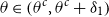

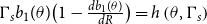


Proof) See Online Appendix B.
The first statement in the proposition shows the existence of the cut-off, above which government accumulates positive reserves. The second statement shows that the optimal reserve accumulation increases in the measure of direct investment inflows, $\theta$
.Footnote
34
Lastly, the third statement shows that the cut-off decreases in the measure of outflow friction
$\theta$
.Footnote
34
Lastly, the third statement shows that the cut-off decreases in the measure of outflow friction $\Gamma _{s}$
.Footnote
35
$\Gamma _{s}$
.Footnote
35
The second statement shows that the sizes of reserve accumulation are bounded below, and the bound increases linearly in $\theta$
. We confirm through various numerical experiments that
$\theta$
. We confirm through various numerical experiments that $\delta _{1}$
is large, and the reserve accumulation is close enough to the lower bound.Footnote
36
That is,
$\delta _{1}$
is large, and the reserve accumulation is close enough to the lower bound.Footnote
36
That is,
 \begin{equation} R^{*}\simeq \left (Q_{0}-A_{0}\right )\left (\theta -\theta ^{c}(\Gamma _{s})\right )K \end{equation}
Equation (16) is the theoretical counterpart to the empirical regularity. From the equation, we can see two comparative statics corresponding to our empirical findings in Section 2. First, the optimal reserve accumulation increases linearly in direct investment inflows once the inflows are beyond the threshold $\theta ^{c}$
. Second, the threshold does depend on the measure of outflow frictions,
$\theta ^{c}$
. Second, the threshold does depend on the measure of outflow frictions, $\Gamma _{s}$
. Therefore, more severe outflow frictions induce more reserve accumulation, given the amounts of direct investment inflows.
$\Gamma _{s}$
. Therefore, more severe outflow frictions induce more reserve accumulation, given the amounts of direct investment inflows.
In our model, the variable $\Gamma _{s}$
is based on two micro-frictions: underdeveloped financial sector and tax evasion through overseas investment (Appendix A). These correspond to our examinations of the financial institution index and the gross capital outflow openness index in the empirical analysis. We view these two frictions as interconnected in practice. Underdeveloped financial sector may be a reason why EMEs impose capital outflow restrictions. Due to their underdeveloped financial sectors, EMEs incur high costs when interacting with international intermediaries to invest abroad. Recognizing this, EM governments implement outflow restrictions to prevent their valuable resources from turning into rents for international intermediaries and to retain beneficial capital within their own borders. Furthermore, overseas investment facilitates tax evasion in underdeveloped countries, raising enforcement costs for the government. This is modeled explicitly in Appendix A. Both these channels provide theoretical underpinnings for why gross capital outflow openness remains limited in many EMEs.
$\Gamma _{s}$
is based on two micro-frictions: underdeveloped financial sector and tax evasion through overseas investment (Appendix A). These correspond to our examinations of the financial institution index and the gross capital outflow openness index in the empirical analysis. We view these two frictions as interconnected in practice. Underdeveloped financial sector may be a reason why EMEs impose capital outflow restrictions. Due to their underdeveloped financial sectors, EMEs incur high costs when interacting with international intermediaries to invest abroad. Recognizing this, EM governments implement outflow restrictions to prevent their valuable resources from turning into rents for international intermediaries and to retain beneficial capital within their own borders. Furthermore, overseas investment facilitates tax evasion in underdeveloped countries, raising enforcement costs for the government. This is modeled explicitly in Appendix A. Both these channels provide theoretical underpinnings for why gross capital outflow openness remains limited in many EMEs.
Overall, once we view direct investment capital flows as exogenous, we can explain the evolution of international reserves of EMEs over the last two decades. That is, as EMEs receive more direct investment flows, many EMEs absorb capital inflows by accumulating reserves.Footnote 37 We summarize the analytical results and the following discussions in the remark below.Footnote 38
Remark 1.
For direct investment inflows beyond a certain level, 1) the government absorbs the extra inflows by accumulating reserves. 2) More outflow friction (higher $\Gamma _{s}$
) induces more reserve accumulation given the amounts of direct investment inflows, as they lower the threshold of direct investment inflows.
$\Gamma _{s}$
) induces more reserve accumulation given the amounts of direct investment inflows, as they lower the threshold of direct investment inflows.
Discussion of currency manipulation Another finding from Proposition 2 is that the real exchange rates in period 0 become insensitive to $\theta$
as the government amasses reserves.
$\theta$
as the government amasses reserves.
 \begin{eqnarray}p_{0} &=& \Big(\frac {1-\alpha }{\alpha }\Big)\frac {y_{0}^{T}+(Q_{0}-A_{0})\theta K+b_{1}(\theta)-R (\theta)}{y_{0}^{N}}\nonumber\\[2pt]&\simeq& \Big(\frac {1-\alpha }{\alpha }\Big)\frac {y_{0}^{T}+(Q_{0}-A_{0})\theta ^{c}(\Gamma _{s})K+b_{1}(\theta ^{c}(\Gamma _{s}))}{y_{0}^{N}} \end{eqnarray}
The expression for $p_{0}$
indicates that it is almost invariant to
$p_{0}$
indicates that it is almost invariant to $\theta \in (\theta ^{c},\;1)$
. When confronted with direct investment flows exceeding a certain threshold, the government “passively” absorbs the additional inflows. Consequently, the real exchange rate appears “invariant” to the inflows from direct investments.
$\theta \in (\theta ^{c},\;1)$
. When confronted with direct investment flows exceeding a certain threshold, the government “passively” absorbs the additional inflows. Consequently, the real exchange rate appears “invariant” to the inflows from direct investments.
Accumulated reserves are often viewed as evidence of currency manipulation intended to gain export competitiveness. For example, one of the criteria that the US Treasury uses to judge whether an EME is manipulating its currency value is the amount of reserve accumulation.Footnote 39 In the literature, it has often been argued that the precautionary view cannot justify international reserve holdings of extraordinarily large sizes, and therefore, large sizes of reserves must be byproducts of the export-oriented growth strategy (i.e., currency manipulationFootnote 40 ).
In contrast, we argue that the simple reserve-to-GDP ratio is not a good measure for identifying a currency manipulation. If excessive reserve accumulation occurs when there are large and exogenous capital inflows, then the purpose of reserve accumulation may not be currency manipulation but consumption smoothing. Our theory explains why the sizes of accumulated reserves are not good “litmus” to test currency manipulation. Proposition 2 implies that EMEs facing massive capital inflows make corresponding capital outflows in the form of reserves to maintain a macroeconomic balance. The purpose of reserve accumulation is to reallocate resources from capital inflows to the future. The government in our model does not have mercantilist motives as we do not include any ingredients related to mercantilism, such as positive externalities from exports.
Figure 5 well illustrates this point. First, in the absence of reserve accumulation, direct investment flows generate consumption booms and appreciate the real exchange rate, similar to Figure 2. Therefore, although direct investments lower the probability of a sudden stop, the probability falls slowly as households cannot invest abroad enough. In contrast, once the planner accumulates reserves in response to the inflows, capital outflows are generated enough by the planner, keeping tradable goods consumption almost constant. Consequently, the real exchange rate is almost constant as well. More importantly, the sudden stop probability decreases much faster. As a result, the equilibrium with reserve accumulation is similar to little or no friction on capital outflows (very small $\Gamma _{s}$
).
$\Gamma _{s}$
).
Reserve accumulation and currency manipulation. Notes: The figure illustrates how reserve accumulation helps replicate the macroeconomic balance that would be achieved under frictionless capital outflows. Parameter values are the same as in the benchmark case. CE and SP refer to the competitive equilibrium without reserve accumulation and the equilibrium with optimal reserve accumulation, respectively.

In this regard, reserve accumulation is a way to “restore” the macroeconomic balance under frictionless capital outflows. The real exchange rate may be an intermediate target for the planner as it measures over-consumption in the present, but the purpose of the intervention is to prevent “appreciation” of the currency, not to “depreciate” the currency. The current account ( $y_{0}^{T}-c_{0}^{T}$
) under reserve accumulation (SP) also resembles that under no reserve accumulation but with little friction (CE,
$y_{0}^{T}-c_{0}^{T}$
) under reserve accumulation (SP) also resembles that under no reserve accumulation but with little friction (CE, $\Gamma =0.01$
).Footnote
41
$\Gamma =0.01$
).Footnote
41
3.4. Reserve accumulation with capital controls
Now, we analyze reserve accumulation in an environment where government has control over capital flows.Footnote 42 The analysis here further elucidates the relationship between capital outflow restrictions and reserve accumulation, presented in Section 2. We only consider capital controls on debt flows. The analysis of the relationship between capital controls on direct investment flows and reserve accumulation is introduced in Online Appendix F.
Suppose government can tax or subsidize (negative tax) debt instrument-type capital flows. As well-known in the literature, the optimal tax can achieve the same equilibrium where government directly chooses the capital flow. The optimal tax is characterized as follows.
 \begin{align} \tau _{b} & =\frac {1}{\mathbb{E}\left [u_{1}^{T}\right ]}\left [\int _{\underline {\phi }}^{\phi ^{c}}-\frac {db_{2}}{db_{1}}u_{1}^{T}{-{\beta }}\Gamma _{j} b_{2}\frac {db_{2}}{db_{1}}u_{2}^{T}d\mathcal{F}_{\phi }\right ] \end{align}
Thus, the optimal tax increases in the externalities from borrowing or saving of households.Footnote 43
Now, we present two equations characterizing the equilibrium where the government optimally accumulates reserves and taxes (or chooses to borrow or save). Assuming an interior solution, the equilibrium is characterized by the following two equations.
 \begin{equation} -u_{0}^{T}+\beta u_{1}^{T}\big(1+r^{*}-2\Gamma _{s}b_{1}^{sp}\big)+\beta \int _{\underline {\phi }}^{\phi ^{c}}(\!-u_{1}^{T}+\beta u_{2}^{T}(1+r_{2}))\frac {db_{2}}{dw_{1}}(1+r^{*}-2\Gamma _{s}b_{1}^{sp})=0 \end{equation}
 \begin{equation} -u_{0}^{T}+\beta u_{1}^{T}(1+\overline {r})+\beta \int _{\underline {\phi }}^{\phi ^{c}}(\!-u_{1}^{T}+\beta u_{2}^{T}(1+r_{2}))\frac {db_{2}}{dw_{1}}\left (1+\overline {r}\right )=0 \end{equation}
where $w_{1}=b_{1}\left (1+r_{1}\right )+R$
and
$w_{1}=b_{1}\left (1+r_{1}\right )+R$
and $b_{2}$
is characterized in Equations (10) and (11). It is straightforward to solve for
$b_{2}$
is characterized in Equations (10) and (11). It is straightforward to solve for $b_{1}^{sp}$
assuming an interior solution for both
$b_{1}^{sp}$
assuming an interior solution for both $b_{1}^{sp}$
and
$b_{1}^{sp}$
and $R$
. Equations (19) and (20) give us
$R$
. Equations (19) and (20) give us
 \begin{align} b_{1}^{sp} & =\frac {r^{*}-\overline {r}}{2\Gamma _{s}} \end{align}
Equation (21) is an interior solution and $b_{1}^{sp}\gt 0$
. This implies that the government does not accumulate reserves if borrowing is the optimal choice. This is because capital control is a superior substitute for reserve accumulation when the optimal decision is to borrow abroad.Footnote
44
$b_{1}^{sp}\gt 0$
. This implies that the government does not accumulate reserves if borrowing is the optimal choice. This is because capital control is a superior substitute for reserve accumulation when the optimal decision is to borrow abroad.Footnote
44
Even when the government chooses to save, if the saving is less than $\frac {r^{*}-\overline {r}}{2\Gamma _{s}}$
, the government does not accumulate reserves as reserve accumulation is still an inferior saving technology than debt instruments. However, if the required saving exceeds
$\frac {r^{*}-\overline {r}}{2\Gamma _{s}}$
, the government does not accumulate reserves as reserve accumulation is still an inferior saving technology than debt instruments. However, if the required saving exceeds $\frac {r^{*}-\overline {r}}{2\Gamma _{s}}$
, then the government does not expand its debt instrument holdings beyond that level. Instead, the government relies on reserve accumulation. This is because the marginal return to debt instruments, after accounting for intermediation costs, decreases with investment. These are summarized below.Footnote
45
$\frac {r^{*}-\overline {r}}{2\Gamma _{s}}$
, then the government does not expand its debt instrument holdings beyond that level. Instead, the government relies on reserve accumulation. This is because the marginal return to debt instruments, after accounting for intermediation costs, decreases with investment. These are summarized below.Footnote
45
Proposition 3.
Suppose the government optimally taxes or subsidizes debt capital flows and let $\hat {b}_{1}$
be the solution of Equation (
19
) without Equation (
20
). Then, we have
$\hat {b}_{1}$
be the solution of Equation (
19
) without Equation (
20
). Then, we have
-
1.
$\hat {b}_{1}=b_{1}\left (\tau _{b}\right )$
-
2. If
$\hat {b}_{1}\lt \frac {r^{*}-\overline {r}}{2\Gamma _{s}}$
, then
$R^{*}=0$
-
3. If
$\hat {b}_{1}\gt \frac {r^{*}-\overline {r}}{2\Gamma _{s}}$
, then
$b_{1}^{sp}=\frac {r^{*}-\overline {r}}{2\Gamma _{s}}$
and
$R^{*}\gt 0$


Proof) See Online Appendix B.
We can formulate this proposition differently with a corollary. It restates that capital control on debt flows always dominates reserve accumulation for the case of borrowing, while reserve accumulation can be more efficient for saving (See Corollary A.1 in Online Appendix B).Footnote 46
An important observation is that the threshold, $\frac {r^{*}-\overline {r}}{2\Gamma _{s}}$
, is inversely related to the outflow friction measure,
$\frac {r^{*}-\overline {r}}{2\Gamma _{s}}$
, is inversely related to the outflow friction measure, $\Gamma _{s}$
. If
$\Gamma _{s}$
. If $\Gamma _{s}$
is large, the marginal benefit of overseas investment falls rapidly and it is more likely that the government accumulates reserves. Another significant observation is that if saving by decentralized households is larger than the threshold, then the optimal policy is a mix of taxation (outflow restriction) and reserve accumulation. We make it clear with the following corollary.
$\Gamma _{s}$
is large, the marginal benefit of overseas investment falls rapidly and it is more likely that the government accumulates reserves. Another significant observation is that if saving by decentralized households is larger than the threshold, then the optimal policy is a mix of taxation (outflow restriction) and reserve accumulation. We make it clear with the following corollary.
Corollary 1.
Suppose government optimally taxes or subsidies debt capital flows and let $b_{1}^{h}$
be the overseas investments by decentralized households. If
$b_{1}^{h}$
be the overseas investments by decentralized households. If $b_{1}^{h}\gt \frac {r^{*}-\overline {r}}{2\Gamma _{s}}$
, then
$b_{1}^{h}\gt \frac {r^{*}-\overline {r}}{2\Gamma _{s}}$
, then $\tau _{b}\gt 0$
and
$\tau _{b}\gt 0$
and $R\gt 0$
. That is, the optimal policy is to accumulate reserves while taxing capital outflows. Proof) It is trivial.
$R\gt 0$
. That is, the optimal policy is to accumulate reserves while taxing capital outflows. Proof) It is trivial.
This analytical result corresponds well with our empirical findings. Proposition 3 and Corollary 1 imply that reserve management policy has a unique role, which capital controls cannot substitute. This contrasts with earlier studies on reserve accumulation such as Arce et al. (Reference Arce, Bengui and Bianchi2019) and Davis et al. (Reference Davis, Fujiwara, Huang and Wang2021) in which the prudential role of reserves can be fully replaced by capital controls. As IMF (2012) documents, however, reserve accumulation is often used with capital controls in many EMEs.Footnote 47 Our theoretical findings suggest that EMEs receiving large direct investment flows driven by global factors may choose to accumulate reserves while restricting private outflows, especially when policymakers are concerned about their low financial development.Footnote 48 Proposition 3 and Corollary 1 show that this policy combination can be optimal when direct investment inflows are large or when outflow frictions are more severe.Footnote 49
4. Conclusion
Policymakers in emerging economies have long been arguing that they have to accumulate reserves in response to capital inflows caused by global factors. Contrary to the prediction of the classical international economic theory, many believe that capital inflows are expansionary.Footnote 50 In their view, capital inflows inflate asset prices, increase credit and consumption, and may contribute to future financial instability. The most favored policy instrument against unwelcome capital inflows has been the FX intervention and reserve accumulation. The policy takes effect by moving resources from the current capital inflow bonanza to the future (hence, inter-temporal consumption smoothing).Footnote 51
We present a novel reserve accumulation theory that elucidates EME policymakers’ claims. In our model, EME policy authorities absorb the pressures from exogenous capital inflows by accumulating international reserves. The small open economy faces massive direct investment inflows and needs to make corresponding capital outflows for consumption smoothing. However, the private sector cannot invest abroad efficiently due to frictions in their overseas investments. These frictions reflect stringent restrictions on residents’ overseas investments and the EMEs’ underdeveloped financial sector. In this context, we show that a central bank can intervene to generate public capital outflows (reserve accumulation), restore macroeconomic balance, and improve inter-temporal resource allocation to mimic a frictionless equilibrium.
Importantly, our theory is grounded in empirical regularities we establish through an investigation of 34 EMEs from 1999 to 2019. Consistent with our theory, we find that EMEs accumulate reserves when they receive exogenous capital inflows: countries with more obstacles in gross capital outflows accumulate higher levels of reserves; direct investment flows are most significant in inducing EMEs to accumulate reserves. These findings suggest that many EME policymakers have already been acting in accordance with the mechanism of our theory, underscoring the importance of understanding reserve accumulation as an effective stabilization policy.
Supplementary material
The supplementary material for this article can be found at https://doi.org/10.1017/S136510052610087X.
Acknowledgements
We appreciate anonymous reviewers for their constructive comments. We thank Joshua Aizenman, Caroline Betts, Sangyup Choi, Olivier Jeanne, Ahrang Lee, Sungwook Park, Romain Ranciere, Inhwan So, Jongchil Son, and Steve Wu for their valuable comments. We would also like to extend our appreciation to the seminar participants at the University of Southern California, the Bank of Korea, the Korea International Finance Research Group, the 2022 Annual Conference of the Korea Money and Finance Association, the National Dong Hwa University, and the 2023 KER International Conference. Youngjin Yun acknowledges that this work was supported by the Ministry of Education of the Republic of Korea and the National Research Foundation of Korea (NRF-2023S1A5A8078470). The views expressed herein are those of the authors and do not necessarily reflect the views of the IMF or Bank of Korea.
Appendix A. Micro-foundation for social cost of overseas investment
This appendix provides micro-foundations for the two types of overseas investment frictions featured in the model. Section A.1 derives the baseline specification with intermediation costs stemming from underdeveloped financial institutions. Section A.2 introduces enforcement costs associated with government audits of external investment, which are abstracted from the baseline model. These two frictions correspond to the empirical proxies used in the analysis in Section 2.
A.1 Cost of overseas investment due to low financial development
There is a limited pool of financial experts who belong to the family of the representative household. The experts have a heterogeneous operation cost to intermediate. Following Fanelli and Straub (Reference Fanelli and Straub2021), let the fixed cost be uniformly distributed among experts; There exists a continuum of experts, labeled by $j\in [0,\infty )$
, and expert
$j\in [0,\infty )$
, and expert $j$
pay a cost of
$j$
pay a cost of $j$
. Furthermore, we assume that the experts of measure
$j$
. Furthermore, we assume that the experts of measure $\chi$
can manage assets by the amount of
$\chi$
can manage assets by the amount of $\xi \chi$
. Then, it implies:
$\xi \chi$
. Then, it implies:
 \begin{equation} \xi \chi =b_{1} \end{equation}
If the equilibrium intermediation fee is determined by the marginal cost of the intermediation, then the return facing households $r_{t+1}$
is
$r_{t+1}$
is
 \begin{equation} r_{t+1}=r^{*}-\Gamma _{s}b_{t+1} \end{equation}
where $\Gamma _{s}=\xi ^{-1}$
and
$\Gamma _{s}=\xi ^{-1}$
and $r^{*}$
is the direct return on overseas investment before paying the intermediation fee.Footnote
52
As a result,
$r^{*}$
is the direct return on overseas investment before paying the intermediation fee.Footnote
52
As a result, $r_{t+1}\lt r^{*}$
if
$r_{t+1}\lt r^{*}$
if $b_{t+1}\gt 0$
. Furthermore, the total operation cost is
$b_{t+1}\gt 0$
. Furthermore, the total operation cost is $\frac {1}{2}\Gamma _{s}b_{t+1}^{2}$
. Since the total return from the overseas investment is
$\frac {1}{2}\Gamma _{s}b_{t+1}^{2}$
. Since the total return from the overseas investment is $b_{t+1}\left (1+r^{*}\right )$
, we end up with Equation (5).
$b_{t+1}\left (1+r^{*}\right )$
, we end up with Equation (5).
The resulting rent of $\frac {1}{2}\Gamma _{s}b_{t+1}^{2}$
belongs to the households, as the financial experts are also members of the representative household. However, in a more realistic heterogeneous agent environment, the rent extraction to the experts probably increases income inequality, which shall be socially undesirable. In another case where foreign financial experts do the intermediation, the rent is just a social cost, which is not considered by decentralized households.
$\frac {1}{2}\Gamma _{s}b_{t+1}^{2}$
belongs to the households, as the financial experts are also members of the representative household. However, in a more realistic heterogeneous agent environment, the rent extraction to the experts probably increases income inequality, which shall be socially undesirable. In another case where foreign financial experts do the intermediation, the rent is just a social cost, which is not considered by decentralized households.
A.2 Tax evasion using overseas investment
Another important cost associated with capital outflows is tax evasion or improper asset concealment through these outflows. This type of cost is especially relevant in EMEs with low-quality institutions. Various studies, such as Perez et al. (Reference Perez, Brada and Drabek2012) and Jansk $\grave{y}$
and Palanskỳ (Reference Janskỳ and Palanskỳ2019), document that the major corporations in the EMEs used FDIs for tax evasion. Fear of such capital migration is a reason for strict capital control measures on outflows, as documented in Fernández et al. (Reference Fernández, Klein, Rebucci, Schindler and Uribe2016).
$\grave{y}$
and Palanskỳ (Reference Janskỳ and Palanskỳ2019), document that the major corporations in the EMEs used FDIs for tax evasion. Fear of such capital migration is a reason for strict capital control measures on outflows, as documented in Fernández et al. (Reference Fernández, Klein, Rebucci, Schindler and Uribe2016).
To reflect such features in EMEs, we model the social costs of overseas investment due to tax evasion using the investments. Following Aizenman and Marion (Reference Aizenman and Marion2004), we posit that there is a cost of collecting taxes. However, we assume that this cost only exists for overseas investments. Let $C_{t}^{1}$
be the cost of collecting tax as follows. In addition, we assume that the cost to audit is realized in the next period.Footnote
53
$C_{t}^{1}$
be the cost of collecting tax as follows. In addition, we assume that the cost to audit is realized in the next period.Footnote
53
 \begin{equation} C_{t}^{1}=\frac {\gamma }{2}b_{t+1}^{2} \:\:\:\:\: ( b_{t+1}\gt 0,\:\: \gamma \gt 0 ). \end{equation}
Hence, the tax collection cost is a quadratic function of overseas investments. There is a cost of auditing the incomes and assets of entities and training officials to equip them with adequate expertise. Such cost is increasing in overseas investments as it is increasingly difficult to audit incomes and assets abroad. One important note regarding the cost is that government expenditures are financed through the lump-sum tax, and thus, decentralized agents do not take account of the costs as they take the amounts of tax as given.Footnote 54
Please note that we model the cost of capital migration or asset concealment as the cost to audit. This approach enables us to derive nice solutions without giving up any relevant insights. We will discuss a micro-foundation for this below. We illustrate how overseas investments give rise to negative externality by reducing government expenditures.Footnote 55
To present our model consistently with this friction, we let $\gamma = \Gamma _{s}$
. This allows us for a nice presentation of “Gamma” model in the spirit of Gabaix and Maggiori (Reference Gabaix and Maggiori2015). Then, Equation (5) can alter to
$\gamma = \Gamma _{s}$
. This allows us for a nice presentation of “Gamma” model in the spirit of Gabaix and Maggiori (Reference Gabaix and Maggiori2015). Then, Equation (5) can alter to
 \begin{equation} b_{t+1}\left (1+r^{*}\right )=\underset {\text{returns to households}}{\underbrace {\phantom {\frac {!}{!}}b_{t+1}\left (1+r_{t+1}\right )}}+\underset {{\text{tax collection cost}}} {\underbrace {\frac {1}{2}\Gamma _{s}b_{t+1}^{2}}}+\underset {\text{intermediation costs}}{\underbrace {\frac {1}{2}\Gamma _{s}b_{t+1}^{2}}} \end{equation}
The return to financial experts in Equation (5) is replaced with the tax collection cost.
Micro-foundation We simplify the model used in Section 3 by removing the credit constraint in Period 1. This allows us to focus on public expenditure, tax collection and what the model in this subsection describes.
The government, or social planner, must finance public expenditure in period 2, requiring tax collection in period 1, which brings the utility from public goods. The tax rate applies to all tradable goods streams, including tradable goods output and gross returns on overseas investments in period 1. Let us assume that the tax rate on tradable goods streams is $t$
. A critical assumption is that public expenditure in period 2 is determined by the amount of taxes collected in period 1. This assumption is realistic for EME governments unable to raise tax rates substantially or borrow from domestic or foreign investors. Households can conceal a portion of their income from overseas investments, and the proportion they conceal is proportional to the size of those investments. If
$t$
. A critical assumption is that public expenditure in period 2 is determined by the amount of taxes collected in period 1. This assumption is realistic for EME governments unable to raise tax rates substantially or borrow from domestic or foreign investors. Households can conceal a portion of their income from overseas investments, and the proportion they conceal is proportional to the size of those investments. If $\mathit{l}$
represents the fraction households can conceal, then
$\mathit{l}$
represents the fraction households can conceal, then
 \begin{equation*} \mathit{l} = \frac {1}{2}\gamma a \end{equation*}
where $a$
is the overseas investments. The government expenditures are as follows.
$a$
is the overseas investments. The government expenditures are as follows.
 \begin{equation*} \ G = \left [y_{1}^{T} + a\left (1 + r_{1} - \mathit{l} \right ) \right ]t \end{equation*}
Subsequently, the marginal decrease of government expenditures in overseas investments is $\gamma a$
, which is not taken into account by the households, as the households take the total tax collections and government expenditures as given.
$\gamma a$
, which is not taken into account by the households, as the households take the total tax collections and government expenditures as given.
To see it more formally, assume the credit constraint in Equation (8) never binds. Then, if the utility from public goods is $u_{G}$
,
$u_{G}$
,
 \begin{equation*} \frac {\partial V}{\partial a} = -u^{\prime }_{G}\gamma a \lt 0 \end{equation*}
where $V$
is the lifetime utility of the households.Footnote
56
Therefore, overseas investments induce social costs that are overlooked by households. If the utility from public goods is a linear function, then resulted specification of overseas investment cost is identical to equation (25).
$V$
is the lifetime utility of the households.Footnote
56
Therefore, overseas investments induce social costs that are overlooked by households. If the utility from public goods is a linear function, then resulted specification of overseas investment cost is identical to equation (25).
In reality, governments in EMEs might replenish the reduced tax revenues by imposing more taxes on domestic consumption and income. Of course, this should create more distortions, which are another form of social costs that are also overlooked by households.


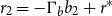


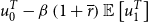


 Open access