

1 INTRODUCTION
There is ample empirical evidence of time-varying parameters in many econometric models (see, e.g., Ghysels and Hall, Reference Ghysels and Hall1990; Inoue and Rossi, Reference Inoue and Rossi2011; Caldara et al., Reference Caldara, Fernández-Villaverde, Rubio-Ramírez and Yao2012; Christoffersen, Jacobs, and Ornthanalai, Reference Christoffersen, Jacobs and Ornthanalai2012; Giacomini and Rossi, Reference Giacomini and Rossi2016). Most studies aiming at accommodating this feature assume a fully parametric model for this time variation; one example of this is structural break models. This has the advantage that the time-varying version of a given model stays parametric and can be estimated using existing methods. The disadvantage is that the researcher runs the risk of choosing a misspecified model for the time variation.
To reduce this risk, methods that treat the problem of time-varying parameters as a structured nonparametric one have been developed: They assume that the sequence of time-varying parameters arise as values of an underlying function which is then estimated nonparametrically; one popular class of estimators that falls in this category are local estimators which includes the so-called rolling-window estimator. However, the existing literature has mostly focused on local constant (Nadaraya–Watson) kernel estimators of the time-varying parameters (see, e.g., Dahlhaus, Richter, and Wu, Reference Dahlhaus, Richter and Wu2019; Bardet, Doukhan, and Wintenberger, Reference Bardet, Doukhan and Wintenberger2022).
We here propose to estimate the time-varying parameters using local polynomial estimators since these are known to have a number of attractive properties compared to the local constant one (see, e.g., Fan, Heckman, and Wand, Reference Fan, Heckman and Wand1995). Under very weak restrictions on the model being estimated and the time-series data being used, we develop an asymptotic theory for the estimators. Specifically, we show that they are normally distributed in large samples and provide a complete characterization of the leading variance and bias components.
The class of estimators includes as special cases the local constant estimator and the local linear estimator. We find that the local constant estimator requires stronger regularity conditions to be well-behaved in large samples and will generally suffer from additional biases in the interior of the domain compared to the local linear estimator. These additional biases involve the so-called time derivative process of the stationary approximation to data which is not present in the biases of the local linear one. Moreover, the local linear estimator enjoys the well-known automatic boundary adjustment property: At the beginning and end of the sample, it will perform better than the local constant one. This feature is important since often the main interest is on the values that the time-varying parameters take at the end of the sample.
The two most closely related papers to ours are Dahlhaus et al. (Reference Dahlhaus, Richter and Wu2019) and Bardet et al. (Reference Bardet, Doukhan and Wintenberger2022) who develop a general theory for local constant estimators of time-varying parameters in Markov models and infinite memory models, respectively. Our general framework encompasses theirs as special cases and we consider a broader class of estimators than they do. Moreover, our proof techniques are different and, when specializing to local constant estimators, allow us to arrive at the same results as they do under weaker conditions: First, our theory imposes minimum requirements on the data-generating process (DGP) with the main assumption being that it is locally stationary. Second, it imposes weaker restrictions on the bandwidth used in the estimation; in particular, we can allow for the bandwidth being chosen using standard bandwidth selection rules, such as cross-validation, which is not the case in Dahlhaus et al. (Reference Dahlhaus, Richter and Wu2019) and Bardet et al. (Reference Bardet, Doukhan and Wintenberger2022). Second, we characterize the leading bias term of the estimators, which is in contrast to Dahlhaus et al. (Reference Dahlhaus, Richter and Wu2019) and Bardet et al. (Reference Bardet, Doukhan and Wintenberger2022). To demonstrate these attractive features of our general theory, we apply it to a class of Markov models with exogenous covariates.
Another important feature of our theory is that it also applies to discrete-valued time-series models, such as Poisson autoregressions. Such models are not covered by the theories of Dahlhaus et al. (Reference Dahlhaus, Richter and Wu2019) and Bardet et al. (Reference Bardet, Doukhan and Wintenberger2022) since these require the DGP to be smooth w.r.t. time which is violated when the time series is discrete-valued. In contrast, our theory for local linear estimators impose very weak smoothness conditions on the DGP due to our new proof techniques and so applies to discrete-valued time-series models without any modifications. For the local constant estimator, we combine the ideas and techniques of Truquet (Reference Truquet2019) with our main result to obtain a complete analysis of this estimator.
We also contribute to the literature on asymptotic analysis of local polynomial estimators of varying-coefficient models by extending existing results (see, e.g., Fan et al., Reference Fan, Heckman and Wand1995; Loader, Reference Loader2006) to cover situations where the objective functions are non-concave. This proves to be a non-trivial extension, but at the same time an important one since the log-likelihood functions of many non-linear models are non-concave.
As an empirical application, we revisit the empirical study of Agosto et al. (Reference Agosto, Cavaliere, Kristensen and Rahbek2016), where a Poisson autoregressive model with additional covariates was used to model and analyze U.S. defaults. Using the proposed methodology, we find substantial time variation in the model parameters that the original study was unable to capture. In particular, we find that the ability of macroeconomic and financial variables to predict defaults have varied substantially over time. A battery of informal tests of the time-varying model against the time-invariant version finds strong support for the former.
The remainder of the article is organized as follows. Framework and estimators are introduced in Section 2. Section 3 presents the asymptotic theory of the estimators. Section 4 provides examples of the theory when applied to particular models. We present the results of two simulation studies and the empirical application in Sections 5 and 6, respectively. We conclude in Section 7, where we discuss how our results potentially could be applied to time-varying infinite-memory models. All proofs have been relegated to the Appendix.
2 FRAMEWORK
We are given n observations,
$Z_{n,t}\in \left ( \mathcal {Z},\left \Vert \cdot \right \Vert \right ) $
 ,
$t=1,\ldots ,n$
,
$t=1,\ldots ,n$
 , where
$\left ( \mathcal {Z} ,\left \Vert \cdot \right \Vert \right ) $
, where
$\left ( \mathcal {Z} ,\left \Vert \cdot \right \Vert \right ) $
 is a Banach space, from a time-series model characterized by a finite-dimensional vector of unknown parameters
$\theta \in \Theta \subset \mathbb {R}^{d_{\theta }}$
is a Banach space, from a time-series model characterized by a finite-dimensional vector of unknown parameters
$\theta \in \Theta \subset \mathbb {R}^{d_{\theta }}$
 to be estimated. In most applications,
$Z_{n,t}$
to be estimated. In most applications,
$Z_{n,t}$
 will also be finite-dimensional but our theory allows for, for example, functional data as well. We take as given an objective function
$\ell _{n,t}\left ( \theta \right ) =\ell \left ( \mathcal {Z}_{n,t};\theta \right ) \in \mathbb {R}$
will also be finite-dimensional but our theory allows for, for example, functional data as well. We take as given an objective function
$\ell _{n,t}\left ( \theta \right ) =\ell \left ( \mathcal {Z}_{n,t};\theta \right ) \in \mathbb {R}$
 , where
$\mathcal {Z} _{n,t}=\left ( Z_{n,t},\dots Z_{n,0},Z_{n,-1},\dots \right ) $
, where
$\mathcal {Z} _{n,t}=\left ( Z_{n,t},\dots Z_{n,0},Z_{n,-1},\dots \right ) $
 . Since we do not observe the process before
$t=1$
. Since we do not observe the process before
$t=1$
 , we here initialize the process at deterministic values chosen by us,
$Z_{n,-t}=z_{-t}$
, we here initialize the process at deterministic values chosen by us,
$Z_{n,-t}=z_{-t}$
 ,
$t\geq 1$
,
$t\geq 1$
 . Under regularity conditions stated below, the effect of the initial values will vanish asymptotically.
The objective function is assumed to identify the data-generating parameter as its maximizer,
$\theta =\arg \max _{\theta ^{\prime }\in \Theta }\mathbb {E} \left [ \ell _{n,t}\left ( \theta ^{\prime }\right ) \right ] $
 , if
$\theta $
, if
$\theta $
 indeed was time-invariant, and
$\ell _{n,t}\left ( \theta ^{\prime }\right ) $
indeed was time-invariant, and
$\ell _{n,t}\left ( \theta ^{\prime }\right ) $
 was stationary and ergodic. In this case, the natural estimator is to replace population expectations by sample ones and estimate
$\theta $
was stationary and ergodic. In this case, the natural estimator is to replace population expectations by sample ones and estimate
$\theta $
 by
$ \hat {\theta }=\arg \max _{\theta ^{\prime }\in \Theta }\frac {1}{n} \sum _{t=1}^{n}\ell _{n,t}\left ( \theta ^{\prime }\right ) $
by
$ \hat {\theta }=\arg \max _{\theta ^{\prime }\in \Theta }\frac {1}{n} \sum _{t=1}^{n}\ell _{n,t}\left ( \theta ^{\prime }\right ) $
 .
.
Suppose now that in fact
$\theta $
 is varying over time so that
$\mathcal {Z} _{n,t}$
is varying over time so that
$\mathcal {Z} _{n,t}$
 is generated by
$\theta _{n,t}=\theta (t/n)$
is generated by
$\theta _{n,t}=\theta (t/n)$
 ,
$t=1,\ldots ,n$
,
$t=1,\ldots ,n$
 , where
$ \theta :\left [ 0,1\right ] \mapsto \Theta $
, where
$ \theta :\left [ 0,1\right ] \mapsto \Theta $
 is an unknown function that characterizes the time variation in the parameters.Footnote
1
At the same time, the objective function is still assumed to identify the parameter in the sense that
$\theta \left ( t/n\right ) =\arg \max _{\theta ^{\prime }\in \Theta }\mathbb {E}\left [ \ell _{n,t}\left ( \theta ^{\prime }\right ) \right ] $
is an unknown function that characterizes the time variation in the parameters.Footnote
1
At the same time, the objective function is still assumed to identify the parameter in the sense that
$\theta \left ( t/n\right ) =\arg \max _{\theta ^{\prime }\in \Theta }\mathbb {E}\left [ \ell _{n,t}\left ( \theta ^{\prime }\right ) \right ] $
 . We then propose to estimate
$\theta \left ( u\right ) $
. We then propose to estimate
$\theta \left ( u\right ) $
 at any given value
$u\in \left [ 0,1\right ] $
at any given value
$u\in \left [ 0,1\right ] $
 using local polynomial estimators: First, for
$t/n$
using local polynomial estimators: First, for
$t/n$
 in a neighborhood of u, we approximate
$\theta \left ( t/n\right ) $
in a neighborhood of u, we approximate
$\theta \left ( t/n\right ) $
 by the following polynomial of order
$m\geq 0$
by the following polynomial of order
$m\geq 0$
 :
:

where
$\beta =\left ( \beta _{1}^{\prime },\ldots ,\beta _{m+1}^{\prime }\right ) ^{\prime }\in \mathbb {R}^{\left ( m+1\right ) d_{\theta }}$
 with
$\beta _{i+1}=\theta ^{\left ( i\right ) }\left ( u\right ) =\partial ^{i}\theta \left ( u\right ) /\partial u^{i}\in \mathbb {R}^{d_{\theta }}$
with
$\beta _{i+1}=\theta ^{\left ( i\right ) }\left ( u\right ) =\partial ^{i}\theta \left ( u\right ) /\partial u^{i}\in \mathbb {R}^{d_{\theta }}$
 and
and

Next, to control the approximation error,
$\theta \left ( t/n\right ) -\theta _{u,\beta }^{\ast }\left ( t/n\right ) $
 , we introduce a kernel weighted version of the “global” objective function evaluated at the polynomial approximation:

where
$K_{b}\left ( \cdot \right ) =K\left ( \cdot /b\right ) /b$
 ,
$K:\mathbb {R} \mapsto \mathbb {R}$
,
$K:\mathbb {R} \mapsto \mathbb {R}$
 is a kernel function, and
$b=b_{n}>0$
is a kernel function, and
$b=b_{n}>0$
 is a bandwidth. The kernel weights ensure that when
$t/n-u$
is a bandwidth. The kernel weights ensure that when
$t/n-u$
 is “large,” the corresponding observations are down weighted in the estimation, thereby controlling for the aforementioned approximation error. We then estimate the polynomial coefficients by

where

The estimated
$\beta $
 coefficients are used as estimates of
$\theta \left ( u\right ) $
coefficients are used as estimates of
$\theta \left ( u\right ) $
 and its first m derivatives,
$\hat {\theta }^{\left ( i\right ) }\left ( u\right ) =\hat {\beta }_{i+1}\left ( u\right ) $
and its first m derivatives,
$\hat {\theta }^{\left ( i\right ) }\left ( u\right ) =\hat {\beta }_{i+1}\left ( u\right ) $
 ,
$i=0,\ldots ,m$
,
$i=0,\ldots ,m$
 . When
$m=0$
. When
$m=0$
 , we recover the standard local-constant estimator. The above class of estimators is similar to the ones considered in Fan et al. (Reference Fan, Heckman and Wand1995) for so-called varying-coefficient models, except that we consider time-series models with the “regressor” that we smooth over being normalized time,
$t/n$
, we recover the standard local-constant estimator. The above class of estimators is similar to the ones considered in Fan et al. (Reference Fan, Heckman and Wand1995) for so-called varying-coefficient models, except that we consider time-series models with the “regressor” that we smooth over being normalized time,
$t/n$
 , and do not restrict
$\theta \mapsto \ell _{n,t}\left ( \theta \right ) $
, and do not restrict
$\theta \mapsto \ell _{n,t}\left ( \theta \right ) $
 to be convex.
The choice of the order of the polynomial, m, should reflect the degree of smoothness that we are willing to assume
$u\mapsto \theta \left ( u\right ) $
 has. If
$\theta \left ( u\right ) $
has. If
$\theta \left ( u\right ) $
 is m times differentiable, then we should use this m in the estimation for optimal control of the bias in the nonparametric estimation. On the other hand, increasing the order of the polynomial tends to increase the variability of the resulting estimator, since more local parameters are introduced in the estimation. For a further discussion of this issue, we refer the reader to Section 3.3 of Fan and Gijbels (Reference Fan and Gijbels2018).
Our framework includes Markov processes and stochastic processes with infinite memory (see, e.g., Doukhan and Wintenberger, Reference Doukhan and Wintenberger2008; Bardet et al., Reference Bardet, Doukhan and Wintenberger2022) as special cases. In Section 4, we apply our general theory to the following class of Markov models with exogenous covariates:

where
$G:\mathcal {Y}^{q}\times \mathcal {X}\times \mathcal {E}\times \Theta $
 is a known function,
$X_{n,t-1}$
is a known function,
$X_{n,t-1}$
 is a Markov process of exogenous covariates, and
$ \varepsilon _{t}$
is a Markov process of exogenous covariates, and
$ \varepsilon _{t}$
 is a sequence of errors. For a given specification of G and the distribution of
$\varepsilon _{t}$
is a sequence of errors. For a given specification of G and the distribution of
$\varepsilon _{t}$
 , we can then derive the corresponding log-likelihood for the model with time-invariant parameters,
$\ell _{n,t}\left ( \theta \right ) =\ell \left ( Z_{n,t},X_{n,t-1};\theta \right ) $
, we can then derive the corresponding log-likelihood for the model with time-invariant parameters,
$\ell _{n,t}\left ( \theta \right ) =\ell \left ( Z_{n,t},X_{n,t-1};\theta \right ) $
 , where
$Z_{n,t}=\left ( Y_{n,t},X_{n,t}\right ) $
, where
$Z_{n,t}=\left ( Y_{n,t},X_{n,t}\right ) $
 . Below, we provide three examples of models that our theory applies to.
Example 1. Time-varying threshold autoregressive with exogenous covariates (tv-TAR-X) model with two regimes:

where
$y^{+}:=\max \left \{ y,0\right \} $
 and
$y^{-}:=\min \left \{ y,0\right \} $
and
$y^{-}:=\min \left \{ y,0\right \} $
 . Here,
$X_{n,t-1}$
. Here,
$X_{n,t-1}$
 contains additional predictors, and
$ \varepsilon _{t}$
contains additional predictors, and
$ \varepsilon _{t}$
 is i.i.d. with
$\mathbb {E}\left [ \varepsilon _{t}\right ] =0 $
is i.i.d. with
$\mathbb {E}\left [ \varepsilon _{t}\right ] =0 $
 and
$\mathbb {E}\left [ \varepsilon _{t}^{2}\right ] <\infty $
and
$\mathbb {E}\left [ \varepsilon _{t}^{2}\right ] <\infty $
 . A natural estimator of
$\theta =\left ( \omega ,\alpha _{1}^{\prime },\alpha _{2}^{\prime },\gamma ^{\prime }\right ) ^{\prime }$
. A natural estimator of
$\theta =\left ( \omega ,\alpha _{1}^{\prime },\alpha _{2}^{\prime },\gamma ^{\prime }\right ) ^{\prime }$
 is the least-squares one so that
$\ell _{n,t}\left ( \theta \right ) =-\left ( Y_{n,t}-\omega -\sum _{i=1}^{q}\alpha _{1,i}Y_{n,t-1}^{+}-\sum _{i=1}^{q}\alpha _{2,i}Y_{n,t-1}^{-}-\gamma ^{\prime }X_{n,t-1}^{-}\right ) ^{2}$
is the least-squares one so that
$\ell _{n,t}\left ( \theta \right ) =-\left ( Y_{n,t}-\omega -\sum _{i=1}^{q}\alpha _{1,i}Y_{n,t-1}^{+}-\sum _{i=1}^{q}\alpha _{2,i}Y_{n,t-1}^{-}-\gamma ^{\prime }X_{n,t-1}^{-}\right ) ^{2}$
 .
.
Example 2. Time-varying ARCH model with covariates (tv-ARCH-X):

where
$\theta =\left ( \omega ,\alpha ^{\prime },\gamma ^{\prime }\right ) ^{\prime }$
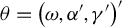 ,
$\varepsilon _{t}$
,
$\varepsilon _{t}$
 is i.i.d. with
$\mathbb {E}\left [ \varepsilon _{t}^{2}\right ] =1,$
is i.i.d. with
$\mathbb {E}\left [ \varepsilon _{t}^{2}\right ] =1,$
 and
$X_{n,t-1}$
and
$X_{n,t-1}$
 contains additional predictors. The Gaussian log-likelihood function takes the form
$\ell _{n,t}\left ( \theta \right ) =-Y_{n,t}/\lambda _{n,t}\left ( \theta \right ) -\log \left ( \lambda _{n,t}\left ( \theta \right ) \right ) $
contains additional predictors. The Gaussian log-likelihood function takes the form
$\ell _{n,t}\left ( \theta \right ) =-Y_{n,t}/\lambda _{n,t}\left ( \theta \right ) -\log \left ( \lambda _{n,t}\left ( \theta \right ) \right ) $
 , where
$\theta =\left ( \omega ,\alpha ^{\prime },\gamma ^{\prime }\right ) ^{\prime }$
, where
$\theta =\left ( \omega ,\alpha ^{\prime },\gamma ^{\prime }\right ) ^{\prime }$
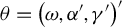 .
.
Example 3. Time-varying Poisson autoregression with exogenous covariates (tv-PARX):

where
$\mathrm {Poisson}\left ( \lambda \right ) $
 denotes the Poisson distribution with intensity parameter
$\lambda $
denotes the Poisson distribution with intensity parameter
$\lambda $
 ,
$\theta =\left ( \omega ,\alpha ^{\prime },\gamma ^{\prime }\right ) ^{\prime }$
,
$\theta =\left ( \omega ,\alpha ^{\prime },\gamma ^{\prime }\right ) ^{\prime }$
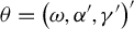 , and
$X_{n,t-1}$
, and
$X_{n,t-1}$
 contains additional predictors. The log-likelihood function takes the form
$ \ell _{n,t}\left ( \theta \right ) =Y_{n,t}\log \left ( \lambda _{n,t}\left ( \theta \right ) \right ) -\lambda _{n,t}\left ( \theta \right ) $
contains additional predictors. The log-likelihood function takes the form
$ \ell _{n,t}\left ( \theta \right ) =Y_{n,t}\log \left ( \lambda _{n,t}\left ( \theta \right ) \right ) -\lambda _{n,t}\left ( \theta \right ) $
 .
.
3 ASYMPTOTIC THEORY
We here provide an asymptotic theory for
$\hat {\beta }$
 . One complication of this analysis is that the components of
$\hat {\beta }$
. One complication of this analysis is that the components of
$\hat {\beta }$
 converge with different rates. We follow the existing literature and handle this issue by introducing a re-scaled version of
$\hat {\beta }$
converge with different rates. We follow the existing literature and handle this issue by introducing a re-scaled version of
$\hat {\beta }$
 (see, e.g., Han and Kristensen, Reference Han and Kristensen2014, for a similar approach): Define
$\hat {\alpha }=U_{n}\hat {\beta }=(\hat {\theta } \left ( u\right ) ^{\prime },b\hat {\theta }^{\left ( 1\right ) }\left ( u\right ) ^{\prime },\ldots ,b^{m}\hat {\theta }^{\left ( m\right ) }\left ( u\right ) ^{\prime })^{\prime }$
(see, e.g., Han and Kristensen, Reference Han and Kristensen2014, for a similar approach): Define
$\hat {\alpha }=U_{n}\hat {\beta }=(\hat {\theta } \left ( u\right ) ^{\prime },b\hat {\theta }^{\left ( 1\right ) }\left ( u\right ) ^{\prime },\ldots ,b^{m}\hat {\theta }^{\left ( m\right ) }\left ( u\right ) ^{\prime })^{\prime }$
 , where

is a weighting matrix containing their relative convergence rates, Given that
$U_{n}$
 is non-singular, the estimation problem (2) is equivalent to solving

where
$D_{m,b}\left ( u\right ) =D_{m}\left ( u/b\right ) $
 and
and

with
$\mathcal {K}$
 denoting the support of K. We will then analyze the properties of
$\hat {\alpha }$
denoting the support of K. We will then analyze the properties of
$\hat {\alpha }$
 .
.
Due to the time-varying parameters,
$Z_{n,t}$
 will generally be non-stationary. To develop an asymptotic theory that allows for this feature, we will rely on the concept of local stationarity as introduced by Dahlhaus (Reference Dahlhaus1997); see also Dahlhaus and Subba Rao (Reference Dahlhaus and Subba Rao2006) and Dahlhaus et al. (Reference Dahlhaus, Richter and Wu2019). We first generalize this concept to sequences of random functions.
Definition 1. A triangular family of random sequences
$W_{n,t}\left ( \theta \right ) $
 ,
$\theta \in \Theta $
,
$\theta \in \Theta $
 ,
$t=1,2,\ldots ,n$
,
$t=1,2,\ldots ,n$
 and
$n\geq 1$
and
$n\geq 1$
 , is uniformly locally stationary on
$\Theta $
, is uniformly locally stationary on
$\Theta $
 (ULS
$\left (p,r,\Theta \right ) $
(ULS
$\left (p,r,\Theta \right ) $
 ) for some
$ p,r>0$
) for some
$ p,r>0$
 if there exists a family of processes
$W_{t}^{\ast }\left ( \theta |u\right ) $
if there exists a family of processes
$W_{t}^{\ast }\left ( \theta |u\right ) $
 ,
$u\in \left [ 0,1\right ] $
,
$u\in \left [ 0,1\right ] $
 , such that: (i) the process
$\left \{ W_{t}^{\ast }\left ( \theta |u\right ) \right \} $
, such that: (i) the process
$\left \{ W_{t}^{\ast }\left ( \theta |u\right ) \right \} $
 is stationary and ergodic for all
$\left ( \theta ,u\right ) \in \Theta \times \left [ 0,1\right ] $
is stationary and ergodic for all
$\left ( \theta ,u\right ) \in \Theta \times \left [ 0,1\right ] $
 and (ii) for some
$C<\infty $
and (ii) for some
$C<\infty $
 and
$\rho <1$
and
$\rho <1$
 ,
,

If
$W_{n,t}\left ( \theta \right ) =W_{n,t}$
 does not depend on any parameters, we write LS
$\left ( p,r\right ) $
does not depend on any parameters, we write LS
$\left ( p,r\right ) $
 . The above condition states that
$W_{n,t}\left ( \theta \right ) $
. The above condition states that
$W_{n,t}\left ( \theta \right ) $
 may be non-stationary, but it is locally in time well-approximated by a stationary version
$W_{t}^{\ast }\left ( \theta |u\right ) $
may be non-stationary, but it is locally in time well-approximated by a stationary version
$W_{t}^{\ast }\left ( \theta |u\right ) $
 . Compared to existing definitions of local stationarity, we allow for an additional term
$\rho ^{t}$
. Compared to existing definitions of local stationarity, we allow for an additional term
$\rho ^{t}$
 to appear in the approximation error. This is needed in order to allow for the initial value of
$ W_{n,t}\left ( \theta \right ) $
to appear in the approximation error. This is needed in order to allow for the initial value of
$ W_{n,t}\left ( \theta \right ) $
 to be chosen arbitrarily. In contrast, by not including
$\rho ^{t}$
to be chosen arbitrarily. In contrast, by not including
$\rho ^{t}$
 in their definitions, most of the existing literature implicitly assumes that
$W_{n,t}\left ( \theta \right ) $
in their definitions, most of the existing literature implicitly assumes that
$W_{n,t}\left ( \theta \right ) $
 has been initialized at
$W_{n,0}\left ( \theta \right ) =W_{0}^{\ast }\left ( \theta |u\right ) $
has been initialized at
$W_{n,0}\left ( \theta \right ) =W_{0}^{\ast }\left ( \theta |u\right ) $
 . When used in the analysis of local estimators, this latter definition implicitly requires that the DGP changes as the researcher varies u in the local log-likelihood which is a rather peculiar assumption. In contrast, the above definition allows for
$W_{n,0}\left ( \theta \right ) $
. When used in the analysis of local estimators, this latter definition implicitly requires that the DGP changes as the researcher varies u in the local log-likelihood which is a rather peculiar assumption. In contrast, the above definition allows for
$W_{n,0}\left ( \theta \right ) $
 to be initialized at a given fixed value—as long as the impact of this dies out with rate
$\rho $
to be initialized at a given fixed value—as long as the impact of this dies out with rate
$\rho $
 .
.
For an example of how the additional error term appears in autoregressive models, we refer the reader to the proof of Lemma 3 in Section 4 which allows for arbitrary initialization of the DGP. The additional error term due to different initializations is here assumed to decay geometrically and so our definition rules out long-memory-type processes. This is mostly for simplicity and we expect that most of our results can be generalized to allow for slower decay rates.
We will then require that
$\ell _{n,t}\left ( \theta \right ) $
 is ULS
$\left ( p,r,\Theta \right ) $
is ULS
$\left ( p,r,\Theta \right ) $
 with stationary approximation
$\ell _{t}^{\ast }\left ( \theta |u\right ) =\ell \left ( \mathcal {Z}_{t}^{\ast }\left ( u\right ) ,\theta \right ) $
with stationary approximation
$\ell _{t}^{\ast }\left ( \theta |u\right ) =\ell \left ( \mathcal {Z}_{t}^{\ast }\left ( u\right ) ,\theta \right ) $
 , where
$\mathcal {Z}_{t}^{\ast }\left ( u\right ) =\left ( Z_{t}^{\ast }\left ( u\right ) ,\ Z_{t-1}^{\ast }\left ( u\right ),\dots \right ) $
, where
$\mathcal {Z}_{t}^{\ast }\left ( u\right ) =\left ( Z_{t}^{\ast }\left ( u\right ) ,\ Z_{t-1}^{\ast }\left ( u\right ),\dots \right ) $
 is the stationary solution to the model being estimated when
$\theta _{n,t}=\theta \left ( u\right ) $
is the stationary solution to the model being estimated when
$\theta _{n,t}=\theta \left ( u\right ) $
 is constant. To illustrate, consider again (3). Under regularity conditions on G and
$\varepsilon _{t}$
is constant. To illustrate, consider again (3). Under regularity conditions on G and
$\varepsilon _{t}$
 (see Section 4 for details), the stationary solution will in this case take the form

where we impose the high-level condition that the exogenous covariates are locally stationary. If the DGP is locally stationary, it follows under great generality that the likelihood and its derivatives are also locally stationary (cf. Section 4).
The next step in our proof is to establish a uniform law of large numbers (ULLN) for the stationary approximation of
$Q_{n}\left ( \alpha |u\right ) $
 ,
$ Q_{n}^{\ast }\left ( \alpha |u\right ) =\frac {1}{n}\sum _{t=1}^{n}K_{b}\left ( t/n-u\right ) \ell _{t}^{\ast }\left ( D_{b}\left ( t/n-u\right ) \alpha |u\right ) $
,
$ Q_{n}^{\ast }\left ( \alpha |u\right ) =\frac {1}{n}\sum _{t=1}^{n}K_{b}\left ( t/n-u\right ) \ell _{t}^{\ast }\left ( D_{b}\left ( t/n-u\right ) \alpha |u\right ) $
 . A sufficient condition for a ULLN to hold is that
$\theta \mapsto \ell _{n,t}^{\ast }\left ( \theta |u\right ) $
. A sufficient condition for a ULLN to hold is that
$\theta \mapsto \ell _{n,t}^{\ast }\left ( \theta |u\right ) $
 is
$L_{p}$
is
$L_{p}$
 -continuous.
Definition 2. A stationary process
$W_{t}^{\ast }\left ( \theta |u\right ) $
 is said to be
$L_{p}$
is said to be
$L_{p}$
 -continuous w.r.t.
$\theta $
-continuous w.r.t.
$\theta $
 if
$ \mathbb {E}\left [ \left \Vert W_{t}^{\ast }\left ( \theta |u\right ) \right \Vert ^{p}\right ] <\infty $
if
$ \mathbb {E}\left [ \left \Vert W_{t}^{\ast }\left ( \theta |u\right ) \right \Vert ^{p}\right ] <\infty $
 for all
$\theta \in \Theta $
for all
$\theta \in \Theta $
 and
and

Imposing
$L_{p}$
 -continuity w.r.t.
$\theta $
-continuity w.r.t.
$\theta $
 is weaker than almost surely continuity: If
$\theta \mapsto W_{t}^{\ast }\left ( \theta |u\right ) $
is weaker than almost surely continuity: If
$\theta \mapsto W_{t}^{\ast }\left ( \theta |u\right ) $
 is almost surely continuous with
$\mathbb {E}\left [ \sup _{\theta \in \Theta }\left \Vert W_{t}^{\ast }\left ( \theta |u\right ) \right \Vert ^{p}\right ] <\infty , $
is almost surely continuous with
$\mathbb {E}\left [ \sup _{\theta \in \Theta }\left \Vert W_{t}^{\ast }\left ( \theta |u\right ) \right \Vert ^{p}\right ] <\infty , $
 the process is also
$L_{p}$
the process is also
$L_{p}$
 -continuous since
$DW_{t}(\delta )=\sup _{\Vert \theta -\theta ^{\prime }\Vert \leq \delta }\left \Vert W_{t}^{\ast }\left ( \theta |u\right ) -W_{t}^{\ast }\left ( \theta ^{\prime }|u\right ) \right \Vert ^{p}$
-continuous since
$DW_{t}(\delta )=\sup _{\Vert \theta -\theta ^{\prime }\Vert \leq \delta }\left \Vert W_{t}^{\ast }\left ( \theta |u\right ) -W_{t}^{\ast }\left ( \theta ^{\prime }|u\right ) \right \Vert ^{p}$
 ,
$\delta>0$
,
$\delta>0$
 , will then satisfy
$\lim _{\delta \rightarrow 0}DW_{t}(\delta )=0$
, will then satisfy
$\lim _{\delta \rightarrow 0}DW_{t}(\delta )=0$
 almost surely and so, by dominated convergence,
$\lim _{\delta \rightarrow 0}\mathbb {E}[DW_{t}(\delta )]=0$
almost surely and so, by dominated convergence,
$\lim _{\delta \rightarrow 0}\mathbb {E}[DW_{t}(\delta )]=0$
 . It is easily verified that
$L_{p}$
. It is easily verified that
$L_{p}$
 -continuity w.r.t.
$\theta $
-continuity w.r.t.
$\theta $
 implies stochastic equicontinuity of
$Q_{n}^{\ast }\left ( \alpha |u\right ) $
implies stochastic equicontinuity of
$Q_{n}^{\ast }\left ( \alpha |u\right ) $
 and so a ULLN holds (cf. Lemma A(i) in Appendix A.1).
We are now ready to state the regularity conditions used to show consistency.
Assumption 1. (i)
$K\left ( \cdot \right ) \geq 0$
 has compact support
$ \mathcal {K}$
has compact support
$ \mathcal {K}$
 and
$\int _{-\infty }^{+\infty }K\left ( v\right ) dv=1$
and
$\int _{-\infty }^{+\infty }K\left ( v\right ) dv=1$
 ; (ii) for some
$\Lambda <\infty $
; (ii) for some
$\Lambda <\infty $
 ,
$\left \vert K(v)-K(\tilde {v})\right \vert \leq \Lambda \left \vert v-\tilde {v}\right \vert $
,
$\left \vert K(v)-K(\tilde {v})\right \vert \leq \Lambda \left \vert v-\tilde {v}\right \vert $
 ,
$v,\tilde {v}\in \mathbb {R}$
,
$v,\tilde {v}\in \mathbb {R}$
 ; and (iii)
$v\mapsto \theta \left ( v\right ) $
; and (iii)
$v\mapsto \theta \left ( v\right ) $
 is continuous at u.
Assumption 2. (i)
$\Theta $
 is compact and the true value
$ \theta \left ( u\right ) \in \Theta $
is compact and the true value
$ \theta \left ( u\right ) \in \Theta $
 ; (ii)
$\theta \mapsto \ell _{t}^{\ast }\left ( \theta |u\right ) $
; (ii)
$\theta \mapsto \ell _{t}^{\ast }\left ( \theta |u\right ) $
 is
$L_{1}$
is
$L_{1}$
 -continuous; and (iii)
$\theta \mapsto \mathbb {E}\left [ \ell _{t}^{\ast }\left ( \theta |u\right ) \right ] $
-continuous; and (iii)
$\theta \mapsto \mathbb {E}\left [ \ell _{t}^{\ast }\left ( \theta |u\right ) \right ] $
 has a unique maximum at
$\theta \left ( u\right ) \in \Theta $
has a unique maximum at
$\theta \left ( u\right ) \in \Theta $
 .
.
Assumption 3.
$\ell _{n,t}\left ( \theta \right ) $
 is ULS
$\left ( 1,r,\Theta \right ) $
is ULS
$\left ( 1,r,\Theta \right ) $
 for some
$r>0$
for some
$r>0$
 with stationary approximation
$\ell _{t}^{\ast }\left ( \theta |u\right ) $
with stationary approximation
$\ell _{t}^{\ast }\left ( \theta |u\right ) $
 .
.
Assumption 1(i) imposes stronger than usual assumptions on
$ K$
 and excludes, among others, the Gaussian kernel and higher-order kernels. It includes, on the other hand, the Epanechnikov and the triangular kernel. The restriction that
$K\left ( \cdot \right ) \geq 0$
and excludes, among others, the Gaussian kernel and higher-order kernels. It includes, on the other hand, the Epanechnikov and the triangular kernel. The restriction that
$K\left ( \cdot \right ) \geq 0$
 is used to ensure the identification of the parameters when
$m>0$
is used to ensure the identification of the parameters when
$m>0$
 ; without this, identification is not necessarily guaranteed; see below for further discussion. For the analysis of the local constant estimator (
$m=0$
; without this, identification is not necessarily guaranteed; see below for further discussion. For the analysis of the local constant estimator (
$m=0$
 ), all subsequent results will go through with K having full support and taking negative values.
The compact support assumption greatly simplifies our analysis of local polynomial estimation of non-concave models: In order to establish uniform convergence of the likelihood, we require
$\Theta $
 to be compact as is standard in the literature. But under this restriction, it is easily checked that
$D_{m,b}\left ( v\right ) \alpha \notin \Theta $
to be compact as is standard in the literature. But under this restriction, it is easily checked that
$D_{m,b}\left ( v\right ) \alpha \notin \Theta $
 as
$b\rightarrow 0$
as
$b\rightarrow 0$
 for any given
$\alpha =\left ( \alpha _{1},\ldots ,\alpha _{m+1}\right ) $
for any given
$\alpha =\left ( \alpha _{1},\ldots ,\alpha _{m+1}\right ) $
 with
$ \alpha _{i}\neq 0$
with
$ \alpha _{i}\neq 0$
 for some
$i\geq 1$
for some
$i\geq 1$
 and any
$v\neq 0$
and any
$v\neq 0$
 . Thus, to allow for kernels with unbounded support, we would generally need the parameter space
$ \mathcal {A}$
. Thus, to allow for kernels with unbounded support, we would generally need the parameter space
$ \mathcal {A}$
 , as defined in (8), to collapse at
$\left \{ \left ( \alpha _{1},0,\ldots ,0\right ) :\alpha _{1}\in \Theta \right \} $
, as defined in (8), to collapse at
$\left \{ \left ( \alpha _{1},0,\ldots ,0\right ) :\alpha _{1}\in \Theta \right \} $
 as
$ b\rightarrow 0$
as
$ b\rightarrow 0$
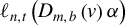
 . Such shrinking behavior in turn means that a formal Taylor expansion of
$\ell _{n,t}\left ( D_{m,b}\left ( v\right ) \alpha \right ) $
. Such shrinking behavior in turn means that a formal Taylor expansion of
$\ell _{n,t}\left ( D_{m,b}\left ( v\right ) \alpha \right ) $
 w.r.t.
$\alpha $
w.r.t.
$\alpha $
 is difficult to obtain and so standard arguments to establish asymptotic normality of
$\hat {\alpha }$
is difficult to obtain and so standard arguments to establish asymptotic normality of
$\hat {\alpha }$
 cannot be applied. On the other hand, by restricting the support
$\mathcal {K}$
cannot be applied. On the other hand, by restricting the support
$\mathcal {K}$
 to be compact,
$ K_{b}\left ( v\right ) \ell _{n,t}\left ( D_{m,b}\left ( v\right ) \alpha \right ) $
to be compact,
$ K_{b}\left ( v\right ) \ell _{n,t}\left ( D_{m,b}\left ( v\right ) \alpha \right ) $
 is well-defined for all
$\alpha \in \mathcal {A}$
is well-defined for all
$\alpha \in \mathcal {A}$
 and
$v\in \mathbb {R}$
and
$v\in \mathbb {R}$
 (where we set
$K_{b}\left ( v\right ) \ell _{n,t}\left ( D_{m,b}\left ( v\right ) \alpha \right ) =0$
(where we set
$K_{b}\left ( v\right ) \ell _{n,t}\left ( D_{m,b}\left ( v\right ) \alpha \right ) =0$
 for
$v/b\notin \mathcal {K}$
for
$v/b\notin \mathcal {K}$
 ). Moreover,
$\left ( \alpha _{1},0,\ldots ,0\right ) $
). Moreover,
$\left ( \alpha _{1},0,\ldots ,0\right ) $
 is an interior point of
$\mathcal {A,}$
is an interior point of
$\mathcal {A,}$
 and so in our analysis of
$\hat {\alpha ,}$
and so in our analysis of
$\hat {\alpha ,}$
 we can employ standard arguments involving a Taylor expansion of the score function around this point.
Assumption 2 is standard in the analysis of “global” extremum estimators of stationary models on the form
$\tilde {\theta }\left ( u\right ) =\arg \max _{\theta \in \Theta }\sum _{t=1}^{n}\ell _{t}^{\ast }\left ( \theta |u\right ) /n$
 . In particular, for a given time-series model, we can import existing results for verification of Assumption 2 (ii) and (iii); see Section 4 for more details. Assumption 2 in conjunction with
$K\left ( \cdot \right ) \geq 0$
. In particular, for a given time-series model, we can import existing results for verification of Assumption 2 (ii) and (iii); see Section 4 for more details. Assumption 2 in conjunction with
$K\left ( \cdot \right ) \geq 0$
 ensures that the local polynomial estimator identifies
$\theta \left ( u\right ) $
ensures that the local polynomial estimator identifies
$\theta \left ( u\right ) $
 . If we allow for kernels that take negative values, we have to replace Assumption 2(iii) with the following more abstract identification condition: The function
$Q^{\ast }\left ( \alpha |u\right ) =\int K\left ( v\right ) \mathbb {E}\left [ \ell _{t}^{\ast }\left ( D_{m}\left ( v\right ) \alpha |u\right ) \right ] dv$
. If we allow for kernels that take negative values, we have to replace Assumption 2(iii) with the following more abstract identification condition: The function
$Q^{\ast }\left ( \alpha |u\right ) =\int K\left ( v\right ) \mathbb {E}\left [ \ell _{t}^{\ast }\left ( D_{m}\left ( v\right ) \alpha |u\right ) \right ] dv$
 satisfies
$Q^{\ast }\left ( \alpha |u\right ) <Q^{\ast }\left ( \left ( \theta \left ( u\right ) ,0,\ldots ,0\right ) |u\right ) $
satisfies
$Q^{\ast }\left ( \alpha |u\right ) <Q^{\ast }\left ( \left ( \theta \left ( u\right ) ,0,\ldots ,0\right ) |u\right ) $
 for any
$\alpha \neq \left ( \theta \left ( u\right ) ,0,\ldots ,0\right ) $
for any
$\alpha \neq \left ( \theta \left ( u\right ) ,0,\ldots ,0\right ) $
 . We have not been able to provide primitive conditions for this to hold when K can take negative values and so instead impose the positivity constraint on K.
If the objective function
$\theta \mapsto \ell _{n,t}\left ( \theta \right ) $
 is concave and
$\Theta $
is concave and
$\Theta $
 is convex, we can replace Assumption 3 with the following pointwise versions: For any
$\theta \in \Theta $
is convex, we can replace Assumption 3 with the following pointwise versions: For any
$\theta \in \Theta $
 ,
$\ell _{n,t}\left ( \theta \right ) $
,
$\ell _{n,t}\left ( \theta \right ) $
 is locally stationary and
$\mathbb {E}\left [ |\ell _{t}^{\ast }\left ( \theta |u\right ) |\right ] <\infty $
is locally stationary and
$\mathbb {E}\left [ |\ell _{t}^{\ast }\left ( \theta |u\right ) |\right ] <\infty $
 (see Theorem 2.7 in Newey and McFadden, Reference Newey and McFadden1994). Under the above assumptions, the following consistency result holds.
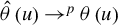
Theorem 1. Let Assumptions 1–3 hold. Then, as
$b\rightarrow 0$
 and
$nb\rightarrow \infty ,\, \hat {\alpha } \rightarrow ^{p}\left ( \theta \left ( u\right ) ,0,\dots ,0\right ) ^{\prime }$
and
$nb\rightarrow \infty ,\, \hat {\alpha } \rightarrow ^{p}\left ( \theta \left ( u\right ) ,0,\dots ,0\right ) ^{\prime }$
 . In particular,
$\hat {\theta }\left ( u\right ) \rightarrow ^{p}\theta \left ( u\right ) $
. In particular,
$\hat {\theta }\left ( u\right ) \rightarrow ^{p}\theta \left ( u\right ) $
 .
.
Note that the above theorem only shows the consistency of
$\hat {\theta }\left ( u\right ) $
 , and so, at this stage, we cannot make any statements regarding
$ \hat {\theta }^{\left ( i\right ) }\left ( u\right ) $
, and so, at this stage, we cannot make any statements regarding
$ \hat {\theta }^{\left ( i\right ) }\left ( u\right ) $
 ,
$i=1,\ldots ,m$
,
$i=1,\ldots ,m$
 . This is similar to other results for nonlinear extremum estimators that converge with different rates (see, e.g., Theorem 9 in Han and Kristensen, Reference Han and Kristensen2014, where a global consistency result is only provided for the component with the fastest rate).
However, under additional regularity conditions on the quasi-likelihood function, we can provide a more precise analysis of the estimators, including local consistency of
$\hat {\theta }^{\left ( k\right ) }\left ( u\right ) $
 ,
$1\leq k\leq m$
,
$1\leq k\leq m$
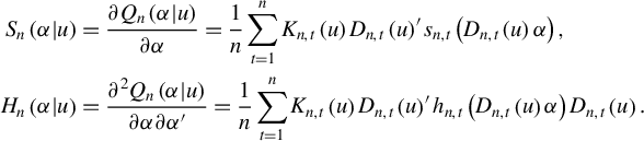
 . With
$s_{n,t}\left ( \theta \right ) =\partial \ell _{n,t}\left ( \theta \right ) /\left ( \partial \theta \right ) \in \mathbb { R}^{d_{\theta }}$
. With
$s_{n,t}\left ( \theta \right ) =\partial \ell _{n,t}\left ( \theta \right ) /\left ( \partial \theta \right ) \in \mathbb { R}^{d_{\theta }}$
 and
$h_{n,t}\left ( \theta \right ) =\partial ^{2}\ell _{n,t}\left ( \theta \right ) /(\partial \theta \partial \theta ^{^{\prime }})\in \mathbb {R}^{d_{\theta }\times d_{\theta }}$
and
$h_{n,t}\left ( \theta \right ) =\partial ^{2}\ell _{n,t}\left ( \theta \right ) /(\partial \theta \partial \theta ^{^{\prime }})\in \mathbb {R}^{d_{\theta }\times d_{\theta }}$
 ,
$D_{n,t}\left ( u\right ) =D_{m,b}\left ( t/n-u\right ) $
,
$D_{n,t}\left ( u\right ) =D_{m,b}\left ( t/n-u\right ) $
 and
$K_{n,t}\left ( u\right ) =K_{b}(t/n-u)$
and
$K_{n,t}\left ( u\right ) =K_{b}(t/n-u)$
 , the score and Hessian of
$Q_{n}\left ( \alpha |u\right ) $
, the score and Hessian of
$Q_{n}\left ( \alpha |u\right ) $
 are given by
It is easily checked that
$\alpha _{0}:=U_{n}\beta _{0}$
 , where
$\beta _{0}=(\theta \left ( u\right ) ^{\prime },\theta ^{\left ( 1\right ) }\left ( u\right ) ^{\prime },\ldots ,\theta ^{\left ( m\right ) }\left ( u\right ) ^{\prime })^{\prime }$
, where
$\beta _{0}=(\theta \left ( u\right ) ^{\prime },\theta ^{\left ( 1\right ) }\left ( u\right ) ^{\prime },\ldots ,\theta ^{\left ( m\right ) }\left ( u\right ) ^{\prime })^{\prime }$
 , belongs to the interior of
$\mathcal {A}$
, belongs to the interior of
$\mathcal {A}$
 for all n large enough due to Assumption 4(ii) below in conjunction with Assumption 2. Due to the consistency result, so will
$\hat {\alpha }$
for all n large enough due to Assumption 4(ii) below in conjunction with Assumption 2. Due to the consistency result, so will
$\hat {\alpha }$
 w.p.a. 1. Thus,
$\hat {\alpha }$
w.p.a. 1. Thus,
$\hat {\alpha }$
 will satisfy the first-order condition of (7) which combined with the mean-value theorem yields

where
$\bar {\alpha }$
 is situated on the line segment connecting
$\hat {\alpha } $
is situated on the line segment connecting
$\hat {\alpha } $
 and
$\alpha _{0}$
and
$\alpha _{0}$
 . We then decompose the score function into a bias and variance component,
$S_{n}\left ( \alpha _{0}|u\right ) =B_{n}\left ( u\right ) +S_{n}\left ( u\right ) $
. We then decompose the score function into a bias and variance component,
$S_{n}\left ( \alpha _{0}|u\right ) =B_{n}\left ( u\right ) +S_{n}\left ( u\right ) $
 , where


and
$\theta _{u}^{\ast }\left ( t/n\right ) $
 was defined in eq. (1). This decomposition is different from the one usually employed in the analysis of kernel estimators of time-varying coefficients, where
$ s_{n,t}$
was defined in eq. (1). This decomposition is different from the one usually employed in the analysis of kernel estimators of time-varying coefficients, where
$ s_{n,t}$
 is replaced by the stationary version of the score function evaluated at
$\theta \left ( u\right ) $
is replaced by the stationary version of the score function evaluated at
$\theta \left ( u\right ) $
 ,
$s_{t}^{\ast }\left ( \theta \left ( u\right ) |u\right ) $
,
$s_{t}^{\ast }\left ( \theta \left ( u\right ) |u\right ) $
 (see, e.g., Dahlhaus and Subba Rao, Reference Dahlhaus and Subba Rao2006; Dahlhaus et al., Reference Dahlhaus, Richter and Wu2019). This “usual” choice has the consequence that the corresponding bias term generally involves the time derivative process of the score function and so the resulting analysis tends to impose stronger regularity conditions on the model being estimated. By instead centering the analysis around
$s_{n,t}$
(see, e.g., Dahlhaus and Subba Rao, Reference Dahlhaus and Subba Rao2006; Dahlhaus et al., Reference Dahlhaus, Richter and Wu2019). This “usual” choice has the consequence that the corresponding bias term generally involves the time derivative process of the score function and so the resulting analysis tends to impose stronger regularity conditions on the model being estimated. By instead centering the analysis around
$s_{n,t}$
 , we can obtain the leading term of the bias
$ B_{n}\left ( u\right ) $
, we can obtain the leading term of the bias
$ B_{n}\left ( u\right ) $
 through a standard Taylor expansion w.r.t.
$\theta $
through a standard Taylor expansion w.r.t.
$\theta $
 :
:

Thus, our approach allows for a simpler derivation of the leading bias and variance terms under the following weak regularity conditions.
Assumption 4. (i)
$\theta \mapsto \ell _{n,t}\left ( \theta \right ) $
 is twice continuously differentiable; (ii)
$\theta \left ( u\right ) $
is twice continuously differentiable; (ii)
$\theta \left ( u\right ) $
 lies in the interior of
$\Theta $
lies in the interior of
$\Theta $
 and is
$m+1$
and is
$m+1$
 times continuously differentiable; and (iii)
$s_{n,t}$
times continuously differentiable; and (iii)
$s_{n,t}$
 is a martingale difference (MGD) array w.r.t.
$\mathcal {F} _{n,t}=\mathcal {F}\left \{ Z_{n,t},Z_{n,t-1},\ldots \right \} $
is a martingale difference (MGD) array w.r.t.
$\mathcal {F} _{n,t}=\mathcal {F}\left \{ Z_{n,t},Z_{n,t-1},\ldots \right \} $
 and LS
$\left ( 2,r\right ) $
and LS
$\left ( 2,r\right ) $
 with stationary approximation
$s_{t}^{\ast }\left ( \theta \left ( u\right ) |u\right ) $
with stationary approximation
$s_{t}^{\ast }\left ( \theta \left ( u\right ) |u\right ) $
 for some
$r>0$
for some
$r>0$
 .
.
Assumption 5. (i)
$h_{n,t}\left ( \theta \right ) $
 is ULS
$\left ( 1,r, \mathcal {N}\left ( u,\epsilon \right ) \right ) $
is ULS
$\left ( 1,r, \mathcal {N}\left ( u,\epsilon \right ) \right ) $
 with continuous stationary approximation
$h_{t}^{\ast }\left ( \theta \left ( u\right ) \right ) $
with continuous stationary approximation
$h_{t}^{\ast }\left ( \theta \left ( u\right ) \right ) $
 for some
$r>0$
for some
$r>0$
 , where
$\mathcal {N}\left ( u,\epsilon \right ) :=\left \{ \theta\hspace{-0.5pt} \in\hspace{-0.5pt} \Theta :\left \Vert \theta\hspace{-0.5pt} -\hspace{-0.5pt}\theta \left ( u\right ) \right \Vert\hspace{-0.5pt} <\hspace{-0.5pt}\epsilon \right \} $
, where
$\mathcal {N}\left ( u,\epsilon \right ) :=\left \{ \theta\hspace{-0.5pt} \in\hspace{-0.5pt} \Theta :\left \Vert \theta\hspace{-0.5pt} -\hspace{-0.5pt}\theta \left ( u\right ) \right \Vert\hspace{-0.5pt} <\hspace{-0.5pt}\epsilon \right \} $
 for some arbitrarily small
$\epsilon>0$
for some arbitrarily small
$\epsilon>0$
 and (ii)
$H\left ( u\right ) \equiv \mathbb {E}\left [ h_{t}^{\ast }\left ( \theta (u)|u\right ) \right ] $
and (ii)
$H\left ( u\right ) \equiv \mathbb {E}\left [ h_{t}^{\ast }\left ( \theta (u)|u\right ) \right ] $
 is non-singular.
Similar to Assumption 2, Assumption 4 contains standard regularity conditions used in the analysis of regular parametric estimators on the form
$\tilde {\theta }\left ( u\right ) =\arg \max _{\theta \in \Theta }\sum _{t=1}^{n}\ell _{t}^{\ast }\left ( \theta |u\right ) $
 . At the same time, Assumption 4(iii) is non-standard compared to the existing literature (as discussed above) and allows us to apply a novel martingale central limit theorem for locally stationary sequences to
$S_{n}\left ( u\right ) $
. At the same time, Assumption 4(iii) is non-standard compared to the existing literature (as discussed above) and allows us to apply a novel martingale central limit theorem for locally stationary sequences to
$S_{n}\left ( u\right ) $
 :
:

(see Lemma A(iii) in Appendix A.1). This result can be seen as a generalization of the standard CLT for stationary and ergodic MGDs that allows for locally stationary processes. The MGD assumption amounts to assuming that the time-varying model is correctly specified and has to be verified on a case-by-case basis (see Section 4.2 for examples of this).
Finally, Assumption 5 together with the expansion in eq. ( 12) is used to derive the limits of
$B_{n}\left ( u\right ) $
 and
$H_{n}\left ( \bar {\alpha }|u\right ) $
and
$H_{n}\left ( \bar {\alpha }|u\right ) $
 :
:

where
$\mu _{i}=\int _{\mathbb {R}}K\left ( v\right ) v^{m+i}D_{m}\left ( v\right ) dv$
 and
$\mathbb {K}_{i}=\int _{\mathbb {R}}K^{i}\left ( v\right ) D_{m}\left ( v\right ) D_{m}\left ( v\right ) ^{\prime }dv$
and
$\mathbb {K}_{i}=\int _{\mathbb {R}}K^{i}\left ( v\right ) D_{m}\left ( v\right ) D_{m}\left ( v\right ) ^{\prime }dv$
 ,
$i\geq 1$
,
$i\geq 1$
 . Combining (9), (13), and (14), we obtain the following theorem.
Theorem 2. Suppose that Assumptions 1–5 hold. Then, as
$b\rightarrow 0$
 and
$nb\rightarrow \infty $
and
$nb\rightarrow \infty $
 ,
,

where
$R_{n}=diag\left \{ b^{m+1},b^{m},\ldots ,b\right \} \otimes I_{d_{\theta }}$
 ,
$V(u)=H\left ( u\right ) ^{-1}\Omega \left ( u\right ) H\left ( u\right ) ^{-1}$
,
$V(u)=H\left ( u\right ) ^{-1}\Omega \left ( u\right ) H\left ( u\right ) ^{-1}$
 , and
$Bias\left ( u\right ) =\mathbb {K}_{1}^{-1}\mu _{1}\otimes \frac {\theta ^{\left ( m+1\right ) }\left ( u\right ) }{\left ( m+1\right ) !}$
, and
$Bias\left ( u\right ) =\mathbb {K}_{1}^{-1}\mu _{1}\otimes \frac {\theta ^{\left ( m+1\right ) }\left ( u\right ) }{\left ( m+1\right ) !}$
 .
.
In particular, for
$i=0,1,\ldots ,m$
 ,
,

where
$Bias_{i}\left ( u\right ) =\kappa _{1,i}\frac {\theta ^{\left ( m+1\right ) }\left ( u\right ) }{\left ( m+1\right ) !}$
 and
$\kappa _{1,i}$
and
$\kappa _{1,i}$
 and
$ \kappa _{2,i}$
and
$ \kappa _{2,i}$
 denote the ith element of
$\mathbb {K}_{1}^{-1}\mu _{1}$
denote the ith element of
$\mathbb {K}_{1}^{-1}\mu _{1}$
 and
$\left ( i,i\right ) $
and
$\left ( i,i\right ) $
 th element of
$\mathbb {K}_{1}^{-1}\mathbb {K}_{2}\mathbb {K }_{1}^{-1}$
th element of
$\mathbb {K}_{1}^{-1}\mathbb {K}_{2}\mathbb {K }_{1}^{-1}$
 , respectively.
Similar to existing results for local polynomial estimators in a cross-sectional setting, the leading bias term in (15) only depends on
$\theta ^{\left ( m+1\right ) }\left ( u\right ) $
 and so the estimators adapt to the curvature of
$\theta \left ( u\right ) $
and so the estimators adapt to the curvature of
$\theta \left ( u\right ) $
 . The asymptotic variance in Theorem 2 can be estimated using plug-in methods: It follows from the proof of Theorem 2 that
$ H_{n}\left ( \hat {\alpha }|u\right ) \rightarrow ^{p}\mathbb {K}_{1}\otimes H\left ( u\right ) $
. The asymptotic variance in Theorem 2 can be estimated using plug-in methods: It follows from the proof of Theorem 2 that
$ H_{n}\left ( \hat {\alpha }|u\right ) \rightarrow ^{p}\mathbb {K}_{1}\otimes H\left ( u\right ) $
 and
and

Compared to most existing asymptotic results for the local constant estimator, such as Dahlhaus et al. (Reference Dahlhaus, Richter and Wu2019), the above result with
$m\geq 1$
 imposes much weaker restrictions on the bandwidth. In particular, standard bandwidth selection rules can be employed here but not under most of the existing theories since their conditions require undersmoothing (i.e.,
$ b\rightarrow 0$
imposes much weaker restrictions on the bandwidth. In particular, standard bandwidth selection rules can be employed here but not under most of the existing theories since their conditions require undersmoothing (i.e.,
$ b\rightarrow 0$
 at a faster rate than the optimal one). This is due to the fact that these theories do not provide a complete characterization of the leading bias term. The few papers that do characterize the leading bias term, such as Dahlhaus and Subba Rao (Reference Dahlhaus and Subba Rao2006), require the so-called time derivatives of the stationary score function to exist and be well-behaved since these enter their bias expressions. Our conditions and results, on the other hand, do not require these and are analogous to the ones found in the literature on local polynomial likelihood estimators (see, e.g., Theorem 1b of Fan et al., Reference Fan, Heckman and Wand1995).
Equation (15) holds for any value of
$m\geq 0$
 and
$ i=0,\ldots ,m$
and
$ i=0,\ldots ,m$
 . However, if K is symmetric, then
$\kappa _{1,i}=0$
. However, if K is symmetric, then
$\kappa _{1,i}=0$
 when
$m-i$
when
$m-i$
 is even. In particular, for the local constant estimator (
$m=i=0$
is even. In particular, for the local constant estimator (
$m=i=0$
 ), Theorem 2 only informs us that the bias component of
$\hat {\theta } \left ( u\right ) $
), Theorem 2 only informs us that the bias component of
$\hat {\theta } \left ( u\right ) $
 is
$o_{p}\left ( b\right ) $
is
$o_{p}\left ( b\right ) $
 which is not a sharp rate. To obtain the leading bias term in the cases where
$m-i$
which is not a sharp rate. To obtain the leading bias term in the cases where
$m-i$
 is even, a higher-order expansion of
$b_{n,t}$
is even, a higher-order expansion of
$b_{n,t}$
 in eq. (10) is necessary. This expansion requires additional assumptions involving aforementioned time derivatives and standard derivatives w.r.t.
$\theta $
in eq. (10) is necessary. This expansion requires additional assumptions involving aforementioned time derivatives and standard derivatives w.r.t.
$\theta $
 of
$h_{t}^{\ast }\left ( \theta \left ( u\right ) |u\right ) $
of
$h_{t}^{\ast }\left ( \theta \left ( u\right ) |u\right ) $
 . To present these, we need the following additional concept.
Definition 3. A stationary process
$W_{t}^{\ast }\left ( \theta |u\right ) $
 is said to be
$ L_{p}$
is said to be
$ L_{p}$
 -differentiable w.r.t. u if there exists a stationary and ergodic process
$\partial _{u}W_{t}^{\ast }\left ( \theta |u\right ) $
-differentiable w.r.t. u if there exists a stationary and ergodic process
$\partial _{u}W_{t}^{\ast }\left ( \theta |u\right ) $
 with
$ \mathbb {E}\left [ \left \Vert \partial _{u}W_{t}^{\ast }\left ( \theta |u\right ) \right \Vert ^{p}\right ] <\infty $
with
$ \mathbb {E}\left [ \left \Vert \partial _{u}W_{t}^{\ast }\left ( \theta |u\right ) \right \Vert ^{p}\right ] <\infty $
 such that

Our definition of time differentiability is slightly weaker compared to the one found in Dahlhaus et al. (Reference Dahlhaus, Richter and Wu2019) and other papers where differentiability w.r.t. u has to hold almost surely. With this definition in hand, we are ready to introduce the following additional regularity conditions in order to derive the leading bias term when
$m-i$
 is even.
Assumption 6.
$\partial h_{n,t}\left ( \theta \right ) /\left ( \partial \theta _{i}\right ) $
 exists and is ULS
$\left ( 1,r,\mathcal {N} (u,\epsilon )\right ) $
exists and is ULS
$\left ( 1,r,\mathcal {N} (u,\epsilon )\right ) $
 with
$L_{1}$
with
$L_{1}$
 -continuous stationary approximation
$ \partial h_{t}^{\ast }\left ( \theta |u\right ) /\left ( \partial \theta _{i}\right ) $
-continuous stationary approximation
$ \partial h_{t}^{\ast }\left ( \theta |u\right ) /\left ( \partial \theta _{i}\right ) $
 ,
$i=1,\ldots ,d_{\theta }$
,
$i=1,\ldots ,d_{\theta }$
 .
.
Assumption 7.
$h_{t}^{\ast }\left ( \theta |u\right ) $
 is
$L_{1}$
is
$L_{1}$
 -differentiable w.r.t. u at
$\theta =\theta \left ( u\right ) $
-differentiable w.r.t. u at
$\theta =\theta \left ( u\right ) $
 with time-derivative
$\partial _{u}h_{t}^{\ast }\left ( \theta \left ( u\right ) |u\right ) =\partial h_{t}^{\ast }\left ( \theta |u\right ) /\left ( \partial u\right ) |_{\theta =\theta \left ( u\right ) }\in \mathbb {R}^{d_{\theta }\times d_{\theta }}$
with time-derivative
$\partial _{u}h_{t}^{\ast }\left ( \theta \left ( u\right ) |u\right ) =\partial h_{t}^{\ast }\left ( \theta |u\right ) /\left ( \partial u\right ) |_{\theta =\theta \left ( u\right ) }\in \mathbb {R}^{d_{\theta }\times d_{\theta }}$
 .
.
Assumption 8.
$\sum _{t=1}^{\infty }\left \vert \mathrm {Cov} \left ( h_{ij,0}^{\ast }\left ( \theta \left ( u\right ) |u\right ) ,h_{ij,t}^{\ast }\left ( \theta \left ( u\right ) |u\right ) \right ) \right \vert <\infty $
 ,
$i,j=1,\ldots ,d_{\theta }.$
,
$i,j=1,\ldots ,d_{\theta }.$

The time-derivative
$\partial _{u}h_{t}^{\ast }\left ( \theta |u\right ) $
 will generally involve time derivatives of the underlying stationary approximation of data: If
$h_{t}^{\ast }\left ( \theta |u\right ) =h\left ( \mathcal {Z}_{t}^{\ast }\left ( u\right ) ;\theta \right ) $
will generally involve time derivatives of the underlying stationary approximation of data: If
$h_{t}^{\ast }\left ( \theta |u\right ) =h\left ( \mathcal {Z}_{t}^{\ast }\left ( u\right ) ;\theta \right ) $
 for some function
$ h $
for some function
$ h $
 which is differentiable w.r.t.
$\mathcal {Z}_{t}^{\ast }\left ( u\right ) $
which is differentiable w.r.t.
$\mathcal {Z}_{t}^{\ast }\left ( u\right ) $
 , then it takes the form
$\partial _{u}h_{t}^{\ast }\left ( \theta |u\right ) =\sum _{i=0}^{\infty }\partial h\left ( z_{0},z_{1},z_{2},\dots ;\theta \right ) /\left ( \partial z_{i}\right ) |_{z=\mathcal {Z}_{t}^{\ast }\left ( u\right ) }\times \partial _{u}Z_{t-i}^{\ast }\left ( u\right ) $
, then it takes the form
$\partial _{u}h_{t}^{\ast }\left ( \theta |u\right ) =\sum _{i=0}^{\infty }\partial h\left ( z_{0},z_{1},z_{2},\dots ;\theta \right ) /\left ( \partial z_{i}\right ) |_{z=\mathcal {Z}_{t}^{\ast }\left ( u\right ) }\times \partial _{u}Z_{t-i}^{\ast }\left ( u\right ) $
 , where
$\partial _{u}Z_{i,t}^{\ast }\left ( u\right ) $
, where
$\partial _{u}Z_{i,t}^{\ast }\left ( u\right ) $
 is the time derivative of
$Z_{t}^{\ast }\left ( u\right ) $
is the time derivative of
$Z_{t}^{\ast }\left ( u\right ) $
 . The short memory condition imposed in Assumption 8 is used to control the variance component of the first-order bias term derived in Theorem 2. In Section 4, we use the concept of
$\tau $
. The short memory condition imposed in Assumption 8 is used to control the variance component of the first-order bias term derived in Theorem 2. In Section 4, we use the concept of
$\tau $
 —weak dependence (Doukhan and Wintenberger, Reference Doukhan and Wintenberger2008) to verify Assumption 8.
Under the above additional assumptions, we obtain the following higher-order expansion of the bias component.
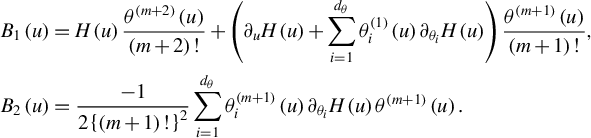
Theorem 3. Suppose Assumptions 1–8 hold and
$\theta \left ( \cdot \right ) $
 is
$m+2$
is
$m+2$
 times continuously differentiable. Then, as
$b\rightarrow 0$
times continuously differentiable. Then, as
$b\rightarrow 0$
 and
$nb\rightarrow \infty $
and
$nb\rightarrow \infty $
 , the bias
$B_{n}\left ( u\right ) $
, the bias
$B_{n}\left ( u\right ) $
 defined in (10) satisfies, with r given in Assumption 6,

where, with
$\partial _{u}H\left ( u\right ) =\mathbb {E}\left [ \partial _{u}h_{t}^{\ast }\left ( \theta |u\right ) \right ] _{\theta =\theta \left ( u\right ) }$
 and
$\partial _{\theta _{i}}H\left ( u\right ) =\mathbb {E}\left [ \partial h_{t}^{\ast }\left ( \theta |u\right ) /\left ( \partial \theta _{i}\right ) \right ] _{\theta =\theta \left ( u\right ) }$
and
$\partial _{\theta _{i}}H\left ( u\right ) =\mathbb {E}\left [ \partial h_{t}^{\ast }\left ( \theta |u\right ) /\left ( \partial \theta _{i}\right ) \right ] _{\theta =\theta \left ( u\right ) }$
 ,
,
As a special case, we obtain the following result for the local constant estimator.
Corollary 1. Under the assumptions of Theorem 3 with
$ m=0$
 together with
$\int _{\mathbb {R}}K\left ( v\right ) vdv=0$
together with
$\int _{\mathbb {R}}K\left ( v\right ) vdv=0$
 , the local constant estimator satisfies, as
$b\rightarrow 0$
, the local constant estimator satisfies, as
$b\rightarrow 0$
 ,
$nb^{3}\rightarrow \infty , $
,
$nb^{3}\rightarrow \infty , $
 and
$n^{\min \left \{ r,1\right \} }b\rightarrow \infty $
and
$n^{\min \left \{ r,1\right \} }b\rightarrow \infty $
 ,
,

where
$Bias_{0}\left ( u\right ) =H^{-1}\left ( u\right ) \left [ B_{1}(u)+B_{2}\left ( u\right ) \right ] $
 and
$B_{1}(u)$
and
$B_{1}(u)$
 and
$B_{2}(u)$
and
$B_{2}(u)$
 are given in Theorem 3.
Two equivalent representations of
$B_{1}(u)+B_{2}\left ( u\right ) $
 are, with
$s_{t}^{\ast }\left ( \theta |u\right ) $
are, with
$s_{t}^{\ast }\left ( \theta |u\right ) $
 denoting the stationary approximation of
$s_{n,t}\left ( \theta \right ) $
denoting the stationary approximation of
$s_{n,t}\left ( \theta \right ) $
 ,
,

where the second representation is only well-defined if
$s_{t}^{\ast }\left ( \theta |u\right ) $
 is twice
$L_{1}$
is twice
$L_{1}$
 -differentiable w.r.t. u.
To our knowledge, this is the first complete characterization of the leading bias term of local constant estimators in general time-varying parameter models. The final characterization of the bias,
$B_{1}(u)+B_{2}\left ( u\right ) =-\frac {1}{2}\partial _{u}^{2}\mathbb {E}\left [ s_{t}^{\ast }\left ( \theta \left ( v\right ) |u\right ) \right ] _{v=u}$
 , corresponds to the one obtained in Dahlhaus and Subba Rao (Reference Dahlhaus and Subba Rao2006) for the time-varying ARCH model. This characterization, however, requires
$s_{t}^{\ast }\left ( \theta |u\right ) $
, corresponds to the one obtained in Dahlhaus and Subba Rao (Reference Dahlhaus and Subba Rao2006) for the time-varying ARCH model. This characterization, however, requires
$s_{t}^{\ast }\left ( \theta |u\right ) $
 to be twice differentiable w.r.t. u, while our characterization only requires
$h_{t}^{\ast }\left ( \theta |u\right ) $
to be twice differentiable w.r.t. u, while our characterization only requires
$h_{t}^{\ast }\left ( \theta |u\right ) $
 to be once differentiable w.r.t. u.
Comparing Theorems 2 and 3, we see that the local linear and local constant estimators share convergence rate and asymptotic variance, but that the latter suffers from additional biases. This is consistent with the theory found for local constant and local linear estimators in a cross-sectional setting (see, e.g., Fan et al., Reference Fan, Heckman and Wand1995).
3.1 Discrete-Valued Time Series
The above theory for the local constant estimator does not cover discrete-valued time-series models. Specifically, Theorem 3 requires
$h_{t}^{\ast }\left ( \theta |u\right ) $
 to be differentiable w.r.t. u (cf. Assumption 7). This property rarely holds when
$h_{t}^{\ast }\left ( \theta |u\right ) $
to be differentiable w.r.t. u (cf. Assumption 7). This property rarely holds when
$h_{t}^{\ast }\left ( \theta |u\right ) $
 is a function of discrete-valued random variables since these are generally not smooth functions of the underlying parameters of the model (see Truquet, Reference Truquet2019 for more details). Thus, Theorem 3 does not apply to, for example, the Poisson autoregressive model.
But Theorem 2 still applies. We therefore combine the ideas of Truquet (Reference Truquet2019, Reference Truquet2020) with Theorem 2 to obtain a theory for the local constant estimator that also covers models with discrete-valued outcomes. This is achieved by replacing Assumptions 7 and 8 with the following ones.
Assumption 9.
$v\mapsto \mathbb {E}\left [ h_{t}^{\ast }\left ( \theta \left ( u\right ) |v\right ) \right ] $
 is continuously differentiable at u.
Assumption 10. (i)
$\bar {V}_{ijkl}\left ( v_{1},v_{2}\right ) :=\sum _{t=1}^{\infty }\mathrm {Cov}\left ( h_{ij,0}^{\ast }\left ( \theta \left ( u\right ) |v_{1}\right ) ,h_{kl,t}^{\ast }\left ( \theta \left ( u\right ) |v_{2}\right ) \right ) $
 exists for all
$\left ( v_{1},v_{2}\right ) $
exists for all
$\left ( v_{1},v_{2}\right ) $
 in a neighborhood of
$\left ( u,u\right ) $
in a neighborhood of
$\left ( u,u\right ) $
 and all
$ \left ( i,j,k,l\right ) $
and all
$ \left ( i,j,k,l\right ) $
 and (ii)
$\bar {V}_{ijkl}\left ( v_{1},v_{2}\right ) $
and (ii)
$\bar {V}_{ijkl}\left ( v_{1},v_{2}\right ) $
 is continuously differentiable at
$\left ( v_{1},v_{2}\right ) =\left ( u,u\right ) $
is continuously differentiable at
$\left ( v_{1},v_{2}\right ) =\left ( u,u\right ) $
 .
.
If
$v\mapsto h_{t}^{\ast }\left ( \theta \left ( u\right ) |v\right ) $
 is
$ L_{1} $
is
$ L_{1} $
 -differentiable w.r.t. v at u, then
$\partial _{v}\mathbb {E}\left [ h_{t}^{\ast }\left ( \theta \left ( u\right ) |v\right ) \right ] _{v=u}=\mathbb {E }\left [ \partial _{v}h_{t}^{\ast }\left ( \theta \left ( u\right ) |v\right ) \right ] _{v=u}$
-differentiable w.r.t. v at u, then
$\partial _{v}\mathbb {E}\left [ h_{t}^{\ast }\left ( \theta \left ( u\right ) |v\right ) \right ] _{v=u}=\mathbb {E }\left [ \partial _{v}h_{t}^{\ast }\left ( \theta \left ( u\right ) |v\right ) \right ] _{v=u}$
 . Thus, Assumption 9 is weaker than Assumption 7 and is satisfied as long as the cumulative distribution function of
$h_{t}^{\ast }\left ( \theta \left ( u\right ) |v\right ) $
. Thus, Assumption 9 is weaker than Assumption 7 and is satisfied as long as the cumulative distribution function of
$h_{t}^{\ast }\left ( \theta \left ( u\right ) |v\right ) $
 is differentiable w.r.t. v (cf. Lemma 2 below). This property holds for many discrete-valued models, including Poisson autoregressions and dynamic discrete choice models (cf. Truquet, Reference Truquet2019, Reference Truquet2020).
Assumption 10, on the other hand, is stronger than Assumption 8. However, similar to Assumption 8, part (i) is satisfied if
$h_{t}^{\ast }\left ( \theta \left ( u\right ) |v\right ) $
 is
$\tau $
is
$\tau $
 -weakly dependent for v in a neighborhood of u since this in turn implies that the joint process
$ \left ( h_{t}^{\ast }\left ( \theta \left ( u\right ) |v_{1}\right ) ,h_{t}^{\ast }\left ( \theta \left ( u\right ) |v_{2}\right ) \right ) $
-weakly dependent for v in a neighborhood of u since this in turn implies that the joint process
$ \left ( h_{t}^{\ast }\left ( \theta \left ( u\right ) |v_{1}\right ) ,h_{t}^{\ast }\left ( \theta \left ( u\right ) |v_{2}\right ) \right ) $
 is weakly dependent for
$\left ( v_{1},v_{2}\right ) $
is weakly dependent for
$\left ( v_{1},v_{2}\right ) $
 in a neighborhood of
$\left ( u,u\right ) $
in a neighborhood of
$\left ( u,u\right ) $
 . Moreover, part (ii) will hold under the same conditions that ensure Assumption 9 holds, namely, that the joint distribution function of
$\left ( h_{0}^{\ast }\left ( \theta \left ( u\right ) |v_{1}\right ) ,h_{t}^{\ast }\left ( \theta \left ( u\right ) |v_{2}\right ) \right ) $
. Moreover, part (ii) will hold under the same conditions that ensure Assumption 9 holds, namely, that the joint distribution function of
$\left ( h_{0}^{\ast }\left ( \theta \left ( u\right ) |v_{1}\right ) ,h_{t}^{\ast }\left ( \theta \left ( u\right ) |v_{2}\right ) \right ) $
 is differentiable.
The following result shows that the results for the local constant estimator remain essentially the same under Assumptions 9 and 10 in place of Assumptions 7 and 8.
Theorem 4. Suppose Assumptions 1–6, 9, and 10 hold and
$ \theta \left ( \cdot \right ) $
 is
$m+2$
is
$m+2$
 times continuously differentiable. Then the conclusions of Theorem 3 and Corollary 1 still hold, except that
$\partial _{u}H\left ( u\right ) $
times continuously differentiable. Then the conclusions of Theorem 3 and Corollary 1 still hold, except that
$\partial _{u}H\left ( u\right ) $
 in the expression of
$B_{1}\left ( u\right ) $
in the expression of
$B_{1}\left ( u\right ) $
 is now defined as
$\partial _{u}H\left ( u\right ) =\partial _{v}E\left [ h_{t}^{\ast }\left ( \theta \left ( u\right ) |v\right ) \right ] _{v=u}$
is now defined as
$\partial _{u}H\left ( u\right ) =\partial _{v}E\left [ h_{t}^{\ast }\left ( \theta \left ( u\right ) |v\right ) \right ] _{v=u}$
 .
.
3.2 Behavior at Boundary
We have already seen that the local linear estimator has smaller biases than the local constant one in the interior of its domain,
$u\in \left ( 0,1\right ) $
 . Another well-known advantage of the local linear estimators in a cross-sectional setting is that they exhibit automatic boundary carpentering. This property also holds in our setting where the boundaries are
$u=0$
. Another well-known advantage of the local linear estimators in a cross-sectional setting is that they exhibit automatic boundary carpentering. This property also holds in our setting where the boundaries are
$u=0$
 and
$u=1$
and
$u=1$
 . Since the results for
$u=1$
. Since the results for
$u=1$
 are similar, we here only analyze the properties of the local constant (
$m=0$
are similar, we here only analyze the properties of the local constant (
$m=0$
 ) and the local linear (
$ m=1$
) and the local linear (
$ m=1$
 ) estimators at
$u=cb$
) estimators at
$u=cb$
 for some constant
$c>0$
for some constant
$c>0$
 . Combining the intermediate bias–variance analysis carried out in the proofs of Theorem 2 and 3 with the arguments of Fan et al. (Reference Fan, Heckman and Wand1995), we find that the two estimators remain asymptotically normally distributed but their asymptotic biases and variances take different forms.
Corollary 2. Let
$\hat {\theta }_{0}\left ( u\right ) $
 and
$\hat {\theta } _{1}\left ( u\right ) $
and
$\hat {\theta } _{1}\left ( u\right ) $
 be the local constant and local linear estimators, respectively, of
$\theta \left ( u\right ) $
be the local constant and local linear estimators, respectively, of
$\theta \left ( u\right ) $
 . Under the assumptions of Theorem 3 with
$m=1$
. Under the assumptions of Theorem 3 with
$m=1$
 together with
$\mu _{1}=\int _{\mathbb {R}}K\left ( v\right ) vdv=0$
together with
$\mu _{1}=\int _{\mathbb {R}}K\left ( v\right ) vdv=0$
 , as
$b\rightarrow 0$
, as
$b\rightarrow 0$
 ,
$nb^{3}\rightarrow \infty , $
,
$nb^{3}\rightarrow \infty , $
 and
$ n^{\min \left \{ r,1\right \} }b\rightarrow \infty $
and
$ n^{\min \left \{ r,1\right \} }b\rightarrow \infty $
 , and for
$m\in \{0,1\}$
, and for
$m\in \{0,1\}$
 ,
,

where
$V\left ( 0_{+}\right ) =\lim _{u\downarrow 0}V\left ( u\right ) $
 and
and
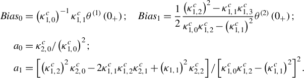
We refer to Fan et al. (Reference Fan, Heckman and Wand1995) for the precise expressions of the constants
$\kappa _{i,j}^{c}$
 ,
$i=1,2$
,
$i=1,2$
 and
$j=0,1,2$
and
$j=0,1,2$
 . At the boundary, both the biases and variances of the local constant and local linear estimators are now different. While the difference between two asymptotic variances is a constant scale, compare
$a_{0}$
. At the boundary, both the biases and variances of the local constant and local linear estimators are now different. While the difference between two asymptotic variances is a constant scale, compare
$a_{0}$
 and
$a_{1}$
and
$a_{1}$
 above, the biases are now of a different order: The local linear estimator still enjoys a bias of order
$ O\left ( b^{2}\right ) $
above, the biases are now of a different order: The local linear estimator still enjoys a bias of order
$ O\left ( b^{2}\right ) $
 while the bias of the local constant one blows up and becomes of order
$O\left ( b\right ) $
while the bias of the local constant one blows up and becomes of order
$O\left ( b\right ) $
 . Thus, the local constant estimator will generally suffer from significantly larger biases at the boundary compared to the local linear one.
4 APPLICATIONS
In this section, we illustrate how our general results can be verified for a class of Markov models with exogenous covariates and provide concrete examples within this framework. Application to infinite-memory models, as considered in Bardet et al. (Reference Bardet, Doukhan and Wintenberger2022), is discussed in Section 7 as a direction for future work.
By inspection of our Assumptions 1–5, we observe that, for a given parametric model and estimator, most of the assumptions are easily verifiable using standard arguments known from the literature on regular parametric estimators. The only ones that are non-standard are Assumptions 3 and 5, which require the researcher to show that
$\ell _{n,t}\left ( \theta \right ) $
 and its first two derivatives are ULS. Similarly, Assumption 6 is also a ULS requirement, while Assumption 8 and/or 10 will hold if
$h_{t}^{\ast }\left ( \theta \left ( u\right ) |u\right ) $
and its first two derivatives are ULS. Similarly, Assumption 6 is also a ULS requirement, while Assumption 8 and/or 10 will hold if
$h_{t}^{\ast }\left ( \theta \left ( u\right ) |u\right ) $
 is weakly dependent.
The following lemma provides sufficient conditions for a given transformation of a time series to be ULS if the underlying time series is ULS. It also shows that if the stationary version is
$\tau $
 -weakly dependent (see Doukhan and Wintenberger, Reference Doukhan and Wintenberger2008 for the definition), then so is the transformation.
Lemma 1. Let
$\left ( \mathcal {Z},\left \Vert \cdot \right \Vert \right ) $
 be a Banach space and
$f:\left ( \mathcal {Z},\left \Vert \cdot \right \Vert \right ) ^{\infty }\times \Theta \mapsto \mathbb {R}^{d}$
be a Banach space and
$f:\left ( \mathcal {Z},\left \Vert \cdot \right \Vert \right ) ^{\infty }\times \Theta \mapsto \mathbb {R}^{d}$
 ,
$ d<\infty $
,
$ d<\infty $
 , be a given mapping. Then the following hold, where
$\mathcal {Z} _{n,t}\left ( \theta \right ) :=\left ( Z_{n,t}\left ( \theta \right ) ,Z_{n,t-1}\left ( \theta \right ) ,\dots \right ) $
, be a given mapping. Then the following hold, where
$\mathcal {Z} _{n,t}\left ( \theta \right ) :=\left ( Z_{n,t}\left ( \theta \right ) ,Z_{n,t-1}\left ( \theta \right ) ,\dots \right ) $
 and
$\mathcal {Z}_{t}^{\ast }\left ( \theta |u\right ) :=\left ( Z_{t}^{\ast }\left ( \theta |u\right ) ,Z_{t-1}^{\ast }\left ( \theta |u\right ) ,\dots \right ) $
and
$\mathcal {Z}_{t}^{\ast }\left ( \theta |u\right ) :=\left ( Z_{t}^{\ast }\left ( \theta |u\right ) ,Z_{t-1}^{\ast }\left ( \theta |u\right ) ,\dots \right ) $
 is its stationary approximation:
-
1. Suppose that (i) for some $g:\left ( \mathcal {Z},\left \Vert \cdot \right \Vert \right ) ^{\infty }\times \Theta \mapsto \mathbb {R}_{+}$
 and
$ \left \{ a_{i}\right \} _{i=0}^{\infty }$
with
$\sum _{i=0}^{\infty }a_{i}<\infty $
so that (17) $$ \begin{align} \left\Vert f(z_{1};\theta )-f(z_{2};\theta )\right\Vert \leq \left\{ \sum_{k=1}^{2}g\left( z_{k}\right) \right\} \sum_{i=0}^{\infty }a_{i}\left\Vert z_{1,i}-z_{2,i}\right\Vert, \end{align} $$
and
$ \left \{ a_{i}\right \} _{i=0}^{\infty }$
with
$\sum _{i=0}^{\infty }a_{i}<\infty $
so that (17) $$ \begin{align} \left\Vert f(z_{1};\theta )-f(z_{2};\theta )\right\Vert \leq \left\{ \sum_{k=1}^{2}g\left( z_{k}\right) \right\} \sum_{i=0}^{\infty }a_{i}\left\Vert z_{1,i}-z_{2,i}\right\Vert, \end{align} $$
for all $\theta \in \Theta $
and
$z_{k}=\left ( z_{k,0},z_{k,1},\ldots \right ) \in \mathcal {Z}^{\infty }$
,
$k=1,2$
and (ii) for some
$p_{1},p_{2}\geq 1$
and
$ r>0$
,
$Z_{n,t}\left ( \theta \right ) \in \mathcal {Z}$
is ULS
$\left ( p_{1},r,\Theta \right ) $
with
$\mathbb {E}\left [ \sup _{\theta \in \Theta }\left \Vert Z_{n,t}\left ( \theta \right ) \right \Vert ^{p_{1}}\right ] <\infty $
,
$\mathbb {E}\left [ \sup _{\theta \in \Theta }g\left ( \mathcal {Z}_{t}^{\ast }\left ( \theta |u\right ) \right ) ^{p_{2}}\right ] <\infty $
and
$\mathbb {E} \left [ \sup _{\theta \in \Theta }g\left ( \mathcal {Z}_{n,t}\left ( \theta \right ) \right ) ^{p_{2}}\right ] <\infty $
. Then
$f\left ( \mathcal {Z} _{n,t}\left ( \theta \right ) ;\theta \right ) $
is ULS
$\left ( p,r,\Theta \right ) $
, where
$p=\left ( 1/p_{1}+1/p_{2}\right ) ^{-1}$
, and
$\mathbb {E} \left [ \sup _{\theta \in \Theta }\left \Vert f\left ( \mathcal {Z}_{t}^{\ast }\left ( \theta \right ) ;\theta \right ) \right \Vert ^{p}\right ] <\infty $
-
2. Suppose that: (i) in part 1. of the lemma holds with (ii’) $g\left ( z\right ) \leq C ( 1+\sum _{i=0}^{\infty } b_{i}\left \Vert z_{i}\right \Vert ^{s} ) $
for some
$s\geq 0$
and
$\left \{ b_{i}\right \} _{i=0}^{\infty }$
with
$\sum _{i=0}^{\infty }b_{i}<\infty $
,
$k=1,2$
; (iii’)
$Z_{n,t}\left ( \theta \right ) \in \mathcal {Z}$
is ULS
$\left ( p_{1},r,\Theta \right ) $
with
$ \mathbb {E}\left [ \sup _{\theta \in \Theta }\left \Vert Z_{n,t}\left ( \theta \right ) \right \Vert ^{p_{1}}\right ] <\infty $
and
$\mathbb {E}\left [ \sup _{\theta \in \Theta }\left \Vert Z_{t}^{\ast }\left ( \theta |u\right ) \right \Vert ^{p_{1}}\right ] <\infty $
, for some
$p_{1}\geq s$
. Then
$f\left ( \mathcal {Z}_{n,t}\left ( \theta \right ) ;\theta \right ) $
is ULS
$\left ( p,r,\Theta \right ) $
with
$\mathbb {E}\left [ \sup _{\theta \in \Theta }\left \Vert f\left ( \mathcal {Z}_{t}^{\ast }\left ( \theta |u\right ) ;\theta \right ) \right \Vert ^{p}\right ] <\infty $
and
$p=p_{1}/\left ( s+1\right ) $
. -
3. Suppose furthermore that $Z_{t}^{\ast }\left ( \theta |u\right ) $
is
$ \tau $
-weakly dependent with weak dependence coefficients
$\tau _{Z}\left ( k\right ) $
. Then
$f\left ( \mathcal {Z}_{t}^{\ast }\left ( \theta |u\right ) ;\theta \right ) $
is also
$\tau $
-weakly dependent with
$\mathbb {E}\left [ \left \Vert f\left ( \mathcal {Z}_{t}^{\ast }\left ( \theta |u\right ) ;\theta \right ) \right \Vert ^{p}\right ] $
whose weak dependence coefficients vanish at the same rate as
$\tau _{Z}\left ( k\right ) $
. In particular, if
$p>2$
and
$\tau _{Z}\left ( k\right ) $
vanish at geometric rate then
$ \sum _{t=1}^{\infty }\left \vert \mathrm {Cov}\left ( f\left ( \mathcal {Z} _{0}^{\ast }\left ( \theta |u\right ) ;\theta \right ) ,f\left ( \mathcal {Z} _{t}^{\ast }\left ( \theta |u\right ) ;\theta \right ) \right ) \right \vert <\infty $
.


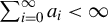








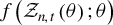






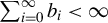





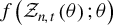





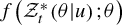





Next, we here provide more primitive conditions for Assumption 9 that can be applied to discrete-valued random variables.
Lemma 2. Suppose that the distribution function
$ F_{Z}\left ( z;u\right ) $
 of
$Z_{t}^{\ast }\left ( u\right ) $
of
$Z_{t}^{\ast }\left ( u\right ) $
 satisfies
$ dF_{Z}\left ( z;u\right ) =p\left ( z;u\right ) d\mu \left ( z\right ) $
satisfies
$ dF_{Z}\left ( z;u\right ) =p\left ( z;u\right ) d\mu \left ( z\right ) $
 for some measure
$\mu $
for some measure
$\mu $
 , where
$u\mapsto p\left ( z;u\right ) $
, where
$u\mapsto p\left ( z;u\right ) $
 is differentiable w.r.t.
$\mu $
is differentiable w.r.t.
$\mu $
 -a.s. Then for any function
$f\left ( z\right ) $
-a.s. Then for any function
$f\left ( z\right ) $
 with
$\mathbb {E }\left [ \left \Vert f\left ( Z_{t}^{\ast }\left (u\right ) ;u\right ) \right \Vert \right ] <\infty $
with
$\mathbb {E }\left [ \left \Vert f\left ( Z_{t}^{\ast }\left (u\right ) ;u\right ) \right \Vert \right ] <\infty $
 ,
$\partial _{u}\mathbb {E}\left [ f\left ( Z_{t}^{\ast }\left (u\right ) \right ) \right ] =\int f\left ( z\right ) \partial _{u}p\left ( z;u\right ) d\mu \left (z\right ) $
,
$\partial _{u}\mathbb {E}\left [ f\left ( Z_{t}^{\ast }\left (u\right ) \right ) \right ] =\int f\left ( z\right ) \partial _{u}p\left ( z;u\right ) d\mu \left (z\right ) $
 assuming the integral is well defined.
A sufficient condition for
$\int \left \vert f\left ( z\right ) \partial _{u}p\left ( zu\right ) \right \vert d\mu \left ( z\right ) <\infty $
 is
$\mathbb { E} [ \left \vert f\left ( Z_{t}^{\ast }\left (u\right ) \right )\right \vert \left \vert s\left ( Z_{t}^{\ast }\left (u\right )\right ) \right \vert ] <\infty $
is
$\mathbb { E} [ \left \vert f\left ( Z_{t}^{\ast }\left (u\right ) \right )\right \vert \left \vert s\left ( Z_{t}^{\ast }\left (u\right )\right ) \right \vert ] <\infty $
 , where
$s = \partial _{u}p/p$
, where
$s = \partial _{u}p/p$
 is the score function. For example, if
$\left \vert s\left ( z;u\right ) \right \vert \leq C\left ( 1+\left \Vert z\right \Vert ^{\delta }\right ) $
is the score function. For example, if
$\left \vert s\left ( z;u\right ) \right \vert \leq C\left ( 1+\left \Vert z\right \Vert ^{\delta }\right ) $
 ,
$\delta \geq 0$
,
$\delta \geq 0$
 , then the result will hold under
$E\left [ \left \Vert Z_{t}^{\ast }\left ( \theta |u\right ) \right \Vert ^{\delta }\left \Vert f\left ( Z_{t}^{\ast }\left ( \theta |u\right ) ;u\right ) \right \Vert \right ] <\infty $
, then the result will hold under
$E\left [ \left \Vert Z_{t}^{\ast }\left ( \theta |u\right ) \right \Vert ^{\delta }\left \Vert f\left ( Z_{t}^{\ast }\left ( \theta |u\right ) ;u\right ) \right \Vert \right ] <\infty $
 . For Markov models, the conditions of Lemma 2 can be verified by importing results from Truquet (Reference Truquet2020) and Vazquez-Abad and Kushner (Reference Vazquez-Abad and Kushner1992); see proof of Corollary 6 for an example of this.
We summarize our findings in the following corollary.
Corollary 3. Suppose that (i) K satisfies Assumption 1; (ii) the stationary version of the model, as summarized by
$\theta \mapsto \ell _{t}^{\ast }\left ( \theta |u\right ) $
 , satisfies Assumptions 2 and 5(ii); (iii)
$s_{n,t}$
, satisfies Assumptions 2 and 5(ii); (iii)
$s_{n,t}$
 is an MGD; (iv)
$\ell _{n,t}\left ( \theta \right )$
is an MGD; (iv)
$\ell _{n,t}\left ( \theta \right )$
 ,
$s_{n,t}$
,
$s_{n,t}$
 , and
$h_n,t(\theta )$
, and
$h_n,t(\theta )$
 satisfy the conditions imposed on f in Lemma 1; (v)
$Z_{n,t}$
satisfy the conditions imposed on f in Lemma 1; (v)
$Z_{n,t}$
 is LS
$\left ( p,r\right ) $
is LS
$\left ( p,r\right ) $
 and
$\mathbb {E}\left [ \left \Vert Z_{t}^{\ast }\left ( u\right ) \right \Vert ^{p}\right ] <\infty $
and
$\mathbb {E}\left [ \left \Vert Z_{t}^{\ast }\left ( u\right ) \right \Vert ^{p}\right ] <\infty $
 . Then, the conclusions of Theorem 2 hold.
Suppose that, in addition, (vi) the stationary distribution satisfies either Assumption 7 or 9; (vii)
$ Z_{t}^{\ast }\left ( u\right ) $
 is
$\tau $
is
$\tau $
 -weakly dependent with
$\tau _{Z}\left ( k\right ) $
-weakly dependent with
$\tau _{Z}\left ( k\right ) $
 vanishing at geometric rate; and (viii)
$h_{t}^{\ast }\left ( \theta |u\right ) $
vanishing at geometric rate; and (viii)
$h_{t}^{\ast }\left ( \theta |u\right ) $
 satisfies (17) with
$\delta \geq 0$
satisfies (17) with
$\delta \geq 0$
 so that
$p/\left ( \delta +1\right )>2$
so that
$p/\left ( \delta +1\right )>2$
 and the conditions of Lemma 2. Then, the conclusions of Theorem 4 hold.
If the model and estimator of interest are regular in the sense that its stationary version satisfies the above assumptions, then all that remains to be shown is that
$Z_{n,t}$
 is locally stationary with
$Z_{t}^{\ast }\left ( u\right ) $
is locally stationary with
$Z_{t}^{\ast }\left ( u\right ) $
 being weakly dependent. The next section provides primitive conditions for this to hold for Markov models with exogenous covariates, while the second section revisits the examples of Section 2 and provides primitive conditions under which our main results apply to these.
4.1 Markov Models with Exogenous Covariates
Consider the following class of q-Markov models with exogenous covariates:


We here restrict
$X_{n,t}$
 to be a Markov process. We could allow for
$ X_{n,t}$
to be a Markov process. We could allow for
$ X_{n,t}$
 to exhibit richer dynamics, for example, allow for
$X_{n,t}$
to exhibit richer dynamics, for example, allow for
$X_{n,t}$
 to depend on lags of
$Y_{n,t}$
to depend on lags of
$Y_{n,t}$
 . However, this would lead to more complicated assumptions and so we here maintain (19) for simplicity. We impose the following assumptions on (18) and (19).
Assumption 11. (i)
$\left ( \varepsilon _{t},\eta _{t}\right ) $
 is i.i.d. over time; (ii) for some
$\rho _{x}<1$
is i.i.d. over time; (ii) for some
$\rho _{x}<1$
 ,
$p\geq 1,$
,
$p\geq 1,$
 and
$x_{0}\in \mathcal {X}^{q}$
and
$x_{0}\in \mathcal {X}^{q}$
 ,
$\mathbb {E}\left [ \left \Vert H\left ( x;\eta _{t},u\right ) -H\left ( \tilde {x};\eta _{t},u\right ) \right \Vert ^{p}\right ] \leq \rho _{x}\left \Vert x-\tilde {x}\right \Vert ^{p}$
,
$\mathbb {E}\left [ \left \Vert H\left ( x;\eta _{t},u\right ) -H\left ( \tilde {x};\eta _{t},u\right ) \right \Vert ^{p}\right ] \leq \rho _{x}\left \Vert x-\tilde {x}\right \Vert ^{p}$
 and
$\mathbb {E}\left [ \left \Vert H\left ( x_{0};\eta _{t},u\right ) \right \Vert ^{p}\right ] <\infty $
and
$\mathbb {E}\left [ \left \Vert H\left ( x_{0};\eta _{t},u\right ) \right \Vert ^{p}\right ] <\infty $
 for all
$ x,x^{\prime }\in \mathcal {X}^{q}$
for all
$ x,x^{\prime }\in \mathcal {X}^{q}$
 and
$u\in \left [ 0,1\right ] $
and
$u\in \left [ 0,1\right ] $
 ; (iii) for some
$\left ( x_{0},y_{0}\right ) \in \mathcal {X}^{q}\times \mathcal {Y}^{q}$
; (iii) for some
$\left ( x_{0},y_{0}\right ) \in \mathcal {X}^{q}\times \mathcal {Y}^{q}$
 ,
$ L<\infty $
,
$ L<\infty $
 and
$\rho _{y}<1$
and
$\rho _{y}<1$
 ,
$\sup _{\theta \in \Theta }\mathbb {E}\left [ \lVert G\left ( y_{0},x_{0},\varepsilon _{t};\theta \right ) \rVert ^{p}\right ] <\infty $
,
$\sup _{\theta \in \Theta }\mathbb {E}\left [ \lVert G\left ( y_{0},x_{0},\varepsilon _{t};\theta \right ) \rVert ^{p}\right ] <\infty $
 and
and

for all
$\left ( x,y\right ) ,\left ( x^{\prime },y^{\prime }\right ) \in \mathcal {X}^{q}\times \mathcal {Y}^{q}$
 ; (iv) for some
$\tilde {p}\geq 1$
; (iv) for some
$\tilde {p}\geq 1$
 ,
$ r>0, $
,
$ r>0, $
 and
$\delta \geq 0$
and
$\delta \geq 0$
 and all
$\theta ,\theta ^{\prime }\in \Theta $
and all
$\theta ,\theta ^{\prime }\in \Theta $
 ,
,


(v)
$\mathbb {E}\left [ \lVert Y_{n,0}\rVert ^{\tilde {p}}\right ] <\infty $
 and
$\mathbb {E}\left [ \lVert X_{n,0}\rVert ^{\tilde {p}}\right ] <\infty $
and
$\mathbb {E}\left [ \lVert X_{n,0}\rVert ^{\tilde {p}}\right ] <\infty $
 .
.
This assumption is similar to the one found in Dahlhaus et al. (Reference Dahlhaus, Richter and Wu2019). However, in contrast to this article, we do not require the process to be initialized at the stationary distribution,
$(Y_{n,0},X_{n,0})=(Y_{0}^{* }\left ( u\right ),X_{0}^{*}\left (u\right ))$
 , and instead allow it to be initialized at any given value or distribution.
Lemma 3. Under Assumption 11(i)–(iii), for any
$u\in \left [ 0,1\right ] $
 , there exists a stationary and
$\tau $
, there exists a stationary and
$\tau $
 -weakly dependent solution
$\left \{ Y_{t}^{\ast }\left ( u\right ) ,X_{t}^{\ast }\left ( u\right ) \right \} $
-weakly dependent solution
$\left \{ Y_{t}^{\ast }\left ( u\right ) ,X_{t}^{\ast }\left ( u\right ) \right \} $
 to
to


with
$\tau _{Y,X}\left ( k\right ) \leq O\left ( \rho ^{k}\right ) $
 . If furthermore Assumption 11(iv) and (v) hold,
$\sup _{u\in \left [ 0,1 \right ] }\mathbb {E}\left [ \lVert X_{t}^{\ast }\left ( u\right ) \rVert ^{ \tilde {p}\delta }\right ] $
. If furthermore Assumption 11(iv) and (v) hold,
$\sup _{u\in \left [ 0,1 \right ] }\mathbb {E}\left [ \lVert X_{t}^{\ast }\left ( u\right ) \rVert ^{ \tilde {p}\delta }\right ] $
 ,
$\sup _{u\in \left [ 0,1\right ] }\mathbb {E}\left [ \lVert Y_{t}^{\ast }\left ( u\right ) \rVert ^{\tilde {p}\delta }\right ] <\infty $
,
$\sup _{u\in \left [ 0,1\right ] }\mathbb {E}\left [ \lVert Y_{t}^{\ast }\left ( u\right ) \rVert ^{\tilde {p}\delta }\right ] <\infty $
 and
$u\mapsto \theta \left ( u\right ) $
and
$u\mapsto \theta \left ( u\right ) $
 and
$u\mapsto H\left ( x,\eta _{t},u\right ) $
and
$u\mapsto H\left ( x,\eta _{t},u\right ) $
 is continuously differentiable, then
$\left ( Y_{n,t},X_{n,t}\right ) $
is continuously differentiable, then
$\left ( Y_{n,t},X_{n,t}\right ) $
 is LS
$\left ( \tilde {p},r\right ) $
is LS
$\left ( \tilde {p},r\right ) $
 with
$\sup _{n,t} \mathbb {E}\left [ \lVert Y_{n,t}\rVert ^{\tilde {p}}\right ] <\infty $
with
$\sup _{n,t} \mathbb {E}\left [ \lVert Y_{n,t}\rVert ^{\tilde {p}}\right ] <\infty $
 and
$ \sup _{n,t}\mathbb {E}\left [ \lVert X_{n,t}\rVert ^{\tilde {p}}\right ] <\infty $
and
$ \sup _{n,t}\mathbb {E}\left [ \lVert X_{n,t}\rVert ^{\tilde {p}}\right ] <\infty $
 for any given initial values
$\left ( Y_{n,0},X_{n,0}\right ) $
for any given initial values
$\left ( Y_{n,0},X_{n,0}\right ) $
 with
$\mathbb {E }\left [ \lVert Y_{n,0}\rVert ^{p}\right ] <\infty $
with
$\mathbb {E }\left [ \lVert Y_{n,0}\rVert ^{p}\right ] <\infty $
 and
$\mathbb {E}\left [ \lVert X_{n,0}\rVert ^{p}\right ] <\infty $
and
$\mathbb {E}\left [ \lVert X_{n,0}\rVert ^{p}\right ] <\infty $
 .
.
Combining Corollary 3 with Lemma 3, we obtain a set of easily verifiable primitive conditions for local M-estimators of time-varying parameters in Markov models to satisfy Theorems 2 and 4 (see Section 4.2 for examples of the verification procedure).
4.2 Specific Examples
We here apply Corollary 3 and Lemma 3 to Examples 1–3. Note here that the first and third examples cannot be analyzed using some of the existing theories since these rely on differentiability of the DGP. Moreover, none of the existing theories allow for covariates to be included in the model. As such, the results below are new to the literature.
Throughout this section, the following assumption is maintained where
$\theta \left ( u\right ) $
 and
$\Theta $
and
$\Theta $
 are specified in each of the following examples.
Assumption 12. (i) The kernel K satisfies Assumption 1; (ii)
$\theta \left ( u\right ) \in \text {Int}\left ( \Theta \right ) $
 and
$\theta \left ( \cdot \right ) $
and
$\theta \left ( \cdot \right ) $
 is twice continuously differentiable; (iii) the additional predictors
$X_{n,t}$
is twice continuously differentiable; (iii) the additional predictors
$X_{n,t}$
 of the model solve (19), where
$H\left ( x,\eta _{\tau };u\right ) $
of the model solve (19), where
$H\left ( x,\eta _{\tau };u\right ) $
 satisfies the conditions in Assumption 11 with
$p=\tilde {p}=2$
satisfies the conditions in Assumption 11 with
$p=\tilde {p}=2$
 ; and (iv)
$\varepsilon _{t}$
; and (iv)
$\varepsilon _{t}$
 is i.i.d.
For the time-varying TAR-X model in Example 1, we obtain the following result.
Corollary 4. Let
$\Theta =\mathbb {R}^{2q+d_{X}+1}$
 and suppose that Assumption 12 holds with
$\mathbb {E}\left [ \varepsilon _{t}^{2}\right ] <\infty $
and suppose that Assumption 12 holds with
$\mathbb {E}\left [ \varepsilon _{t}^{2}\right ] <\infty $
 and
and

Then, the results of Theorem 2 apply to the local linear estimators of the tv-TAR
$(1)$
 model (4) with
$H\left ( u\right ) =\mathbb {E}\left [ \tilde {X}_{t}^{\ast }\left ( u\right ) \tilde {X} _{t}^{\ast }\left ( u\right ) ^{\prime }\right ] $
model (4) with
$H\left ( u\right ) =\mathbb {E}\left [ \tilde {X}_{t}^{\ast }\left ( u\right ) \tilde {X} _{t}^{\ast }\left ( u\right ) ^{\prime }\right ] $
 ,
$\Omega \left ( u\right ) = \mathbb {E}\left [ \varepsilon _{t}^{2}\right ] H\left ( u\right )$
,
$\Omega \left ( u\right ) = \mathbb {E}\left [ \varepsilon _{t}^{2}\right ] H\left ( u\right )$
 , and
, and

If, in addition,
$\mathbb {E}\left [ \varepsilon _{t}^{4}\right ] <\infty $
 ,
$ \varepsilon _{t}$
,
$ \varepsilon _{t}$
 has a differentiable density and
$H\left ( x,\eta _{t},u\right ) $
has a differentiable density and
$H\left ( x,\eta _{t},u\right ) $
 satisfies Assumption 4.1(L3) and (L4) in Dahlhaus et al. (Reference Dahlhaus, Richter and Wu2019), then the results of Theorem 3 hold for the local constant estimators with
$\partial _{\theta }H\left ( u\right ) =0$
satisfies Assumption 4.1(L3) and (L4) in Dahlhaus et al. (Reference Dahlhaus, Richter and Wu2019), then the results of Theorem 3 hold for the local constant estimators with
$\partial _{\theta }H\left ( u\right ) =0$
 and
$\partial _{u}H\left ( u\right ) =\partial H\left ( \theta |u\right ) /\left ( \partial u\right ) |_{\theta =\theta \left ( u\right ) }$
and
$\partial _{u}H\left ( u\right ) =\partial H\left ( \theta |u\right ) /\left ( \partial u\right ) |_{\theta =\theta \left ( u\right ) }$
 .
.
Note here that we do not need to restrict
$\Theta $
 to be compact since here
$\ell _{n,t}\left ( \theta \right ) $
to be compact since here
$\ell _{n,t}\left ( \theta \right ) $
 is concave. Equation (22) ensures that the model indeed has a locally stationary solution and is
$\tau $
is concave. Equation (22) ensures that the model indeed has a locally stationary solution and is
$\tau $
 -weakly dependent. The additional restrictions imposed in the second part of the corollary are used to show that the time derivative of
$\left ( Y_{t}^{\ast }\left ( u\right ) ,X_{t}^{\ast }\left ( u\right ) \right ) $
-weakly dependent. The additional restrictions imposed in the second part of the corollary are used to show that the time derivative of
$\left ( Y_{t}^{\ast }\left ( u\right ) ,X_{t}^{\ast }\left ( u\right ) \right ) $
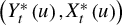 exists so that Assumption 7 holds.
Next, consider the local Gaussian QMLE of the tv-ARCH-X model given in Example 2. Under eq. (23) below, there exists a locally stationary solution to the model which takes the form

where
$\tilde {X}_{t}^{\ast }(u)=\left ( 1,Y_{t-1}^{\ast }(u),\ldots ,Y_{t-q}^{\ast }(u),X_{t-1}^{\ast }\left ( u\right ) ^{\prime }\right ) ^{\prime }$
 .
.
Corollary 5. Assume that Assumption 12 holds,
$\Theta \subseteq \mathbb {R}_{+}^{1+q+d_{X}}$
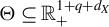 is compact with
$\omega \geq \underline {\omega }>0$
is compact with
$\omega \geq \underline {\omega }>0$
 for all
$\theta \in \Theta $
for all
$\theta \in \Theta $
 ,
$X_{n,t-1}\in \mathbb {R} _{+}^{d_{X}}$
,
$X_{n,t-1}\in \mathbb {R} _{+}^{d_{X}}$
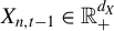 ,
$\mathbb {E}\left [ \varepsilon _{t}^{4}\right ] <\infty $
,
$\mathbb {E}\left [ \varepsilon _{t}^{4}\right ] <\infty $
 ,
$ \inf _{u\in \left [ 0,1\right ] }\omega \left ( u\right )>0,$
,
$ \inf _{u\in \left [ 0,1\right ] }\omega \left ( u\right )>0,$
 and
and
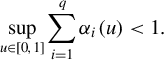
Then, the results of Theorem 2 apply to the local linear estimators of the tv-ARCH-X model (5) with

If, in addition,
$\mathbb {E}\left [ \varepsilon _{t}^{4+\delta }\right ] <\infty $
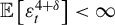 , for some
$\delta>0$
, for some
$\delta>0$
 , and
$H\left ( x,\eta _{t},u\right ) $
, and
$H\left ( x,\eta _{t},u\right ) $
 satisfies Assumption 4.1(L3) and (L4) in Dahlhaus et al. (Reference Dahlhaus, Richter and Wu2019), then the results of Theorem 3 apply to the local constant estimators of the tv-ARCH-X model with
$\partial _{u}H\left ( u\right ) =\partial H\left ( \theta |u\right ) /\left ( \partial u\right ) |_{\theta =\theta \left ( u\right ) }$
satisfies Assumption 4.1(L3) and (L4) in Dahlhaus et al. (Reference Dahlhaus, Richter and Wu2019), then the results of Theorem 3 apply to the local constant estimators of the tv-ARCH-X model with
$\partial _{u}H\left ( u\right ) =\partial H\left ( \theta |u\right ) /\left ( \partial u\right ) |_{\theta =\theta \left ( u\right ) }$
 and
and

Our conditions on the model are more or less identical to Bardet et al. (Reference Bardet, Doukhan and Wintenberger2022) but allows for exogenous regressors to be included. Our conditions are substantially weaker compared to Dahlhaus and Subba Rao (Reference Dahlhaus and Subba Rao2006) and Inoue, Jin, and Pelletier (Reference Inoue, Jin and Pelletier2019) who impose much stronger moment conditions.
Finally, we apply our results to the local MLE of the tv-PARX model in Example 3. Under (24) below, the tv-PARX process is locally stationary with stationary solution
$Y_{t}^{\ast }(u)| \mathcal {F}_{t-1}^{\ast }(u) \sim \mathrm {Poisson}\left ( \lambda _{t}^{\ast }\left ( u\right ) \right ) $
 , where
$\lambda _{t}^{\ast }\left ( u\right ) =\theta \left ( u\right ) ^{\prime }\tilde {X}_{t}^{\ast }\left ( u\right ) $
, where
$\lambda _{t}^{\ast }\left ( u\right ) =\theta \left ( u\right ) ^{\prime }\tilde {X}_{t}^{\ast }\left ( u\right ) $
 and
$\tilde {X}_{t}^{\ast }(u)=\left ( 1,Y_{t-1}^{\ast }(u),\ldots ,Y_{t-q}^{\ast }(u),X_{t-1}^{\ast }\left ( u\right ) ^{\prime }\right ) ^{\prime }$
and
$\tilde {X}_{t}^{\ast }(u)=\left ( 1,Y_{t-1}^{\ast }(u),\ldots ,Y_{t-q}^{\ast }(u),X_{t-1}^{\ast }\left ( u\right ) ^{\prime }\right ) ^{\prime }$
 .
.
Corollary 6. Suppose that Assumption 12 holds,
$\Theta \subseteq \mathbb {R}_{+}^{1+q+d_{X}}$
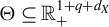 is compact with
$\omega \geq \underline {\omega }>0$
is compact with
$\omega \geq \underline {\omega }>0$
 for all
$\theta \in \Theta $
for all
$\theta \in \Theta $
 ,
$X_{n,t-1}\in \mathbb {R} _{+}^{d_{X}}$
,
$X_{n,t-1}\in \mathbb {R} _{+}^{d_{X}}$
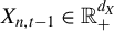 ,
$\inf _{u\in \left [ 0,1\right ] }\omega \left ( u\right )>0,$
,
$\inf _{u\in \left [ 0,1\right ] }\omega \left ( u\right )>0,$
 and
and
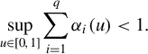
Then, the results of Theorems 2 apply to the local linear estimators of the tv-PARX model (6) with

Suppose furthermore that
$X_{t}^{\ast }\left ( u\right ) $
 satisfies the following: Its Markov transition kernel is continuous w.r.t. the Lebesgue measure with density
$p_{X}\left ( x|x_{0};u\right )>0$
satisfies the following: Its Markov transition kernel is continuous w.r.t. the Lebesgue measure with density
$p_{X}\left ( x|x_{0};u\right )>0$
 which is differentiable w.r.t. u for all
$\left ( x,x_{0}\right ) $
which is differentiable w.r.t. u for all
$\left ( x,x_{0}\right ) $
 ;
$\left \vert \partial _{u}p_{X}\left ( x|x_{0};u\right ) \right \vert /p_{X}\left ( x|x_{0};u\right ) \leq C\left ( 1+\left \Vert x\right \Vert +\left \Vert x_{0}\right \Vert \right ) $
;
$\left \vert \partial _{u}p_{X}\left ( x|x_{0};u\right ) \right \vert /p_{X}\left ( x|x_{0};u\right ) \leq C\left ( 1+\left \Vert x\right \Vert +\left \Vert x_{0}\right \Vert \right ) $
 ;
$p_{X}\left ( x|x_{0};u\right ) \leq \bar {p} _{X}^{\left ( 0\right ) }\left ( x|x_{0};u\right ) $
;
$p_{X}\left ( x|x_{0};u\right ) \leq \bar {p} _{X}^{\left ( 0\right ) }\left ( x|x_{0};u\right ) $
 and
$\left \vert \partial _{u}p_{X}\left ( x|x_{0};u\right ) \right \vert \leq \left \vert \bar {p} _{X}^{\left ( 1\right ) }\left ( x|x_{0}\right ) \right \vert $
and
$\left \vert \partial _{u}p_{X}\left ( x|x_{0};u\right ) \right \vert \leq \left \vert \bar {p} _{X}^{\left ( 1\right ) }\left ( x|x_{0}\right ) \right \vert $
 , where
$\int \left \Vert x\right \Vert ^{2}\bar {p}_{X}^{\left ( k\right ) }\left ( x|x_{0};u\right ) dx<\infty $
, where
$\int \left \Vert x\right \Vert ^{2}\bar {p}_{X}^{\left ( k\right ) }\left ( x|x_{0};u\right ) dx<\infty $
 ,
$k=0,1$
,
$k=0,1$
 . Moreover,
$\mathbb {E}\left [ 1+X_{t}^{\ast }\left ( u\right ) ^{2}|X_{t-1}^{\ast }\left ( u\right ) =x\right ] \leq \rho \left ( u\right ) \left ( 1+\left \Vert x\right \Vert ^{2}\right ) +b\left ( u\right ) $
. Moreover,
$\mathbb {E}\left [ 1+X_{t}^{\ast }\left ( u\right ) ^{2}|X_{t-1}^{\ast }\left ( u\right ) =x\right ] \leq \rho \left ( u\right ) \left ( 1+\left \Vert x\right \Vert ^{2}\right ) +b\left ( u\right ) $
 for some
$\rho \left ( u\right ) <1$
for some
$\rho \left ( u\right ) <1$
 and
$b\left ( u\right ) <\infty $
and
$b\left ( u\right ) <\infty $
 . Then the local constant estimator satisfies Theorem 3 with

5 SIMULATION STUDY
In this section, we examine the finite-sample performances of the local constant and local linear estimators. All reported results are based on 1,000 simulated data sets. The overall performance of the estimators is evaluated using the mean absolute deviation error (MADE),
$MADE_{i}:=\frac {1 }{n}\sum _{t=1}^{n}\mathbb {E}\left [ |\hat {\theta }_{i}\left ( t/n\right ) -\theta _{i}\left ( t/n\right ) |\right ] $
 , as well as their integrated bias, variance, and mean squared error. All results are based on the Epanechnikov kernel and with the bandwidth chosen using the cross-validation method proposed in Richter and Dahlhaus (Reference Richter and Dahlhaus2019).
5.1 Time-Varying ARCH
We first consider the time-varying ARCH(1) in eq. (5), where
$ \varepsilon \sim i.i.d.N\left ( 0,1\right ) $
 ,
$\omega \left ( u\right ) =0.7-0.5\sin \left ( 4\pi u\right ) $
,
$\omega \left ( u\right ) =0.7-0.5\sin \left ( 4\pi u\right ) $
 , and
$\alpha \left ( u\right ) =0.45+0.4\sin \left ( 4\pi u\right ) $
, and
$\alpha \left ( u\right ) =0.45+0.4\sin \left ( 4\pi u\right ) $
 . We estimate
$\omega \left ( u\right ) $
. We estimate
$\omega \left ( u\right ) $
 and
$\alpha \left ( u\right ) $
and
$\alpha \left ( u\right ) $
 using both Gaussian log-likelihood and the WLS method of Fryzlewicz, Sapatinas, and Subba Rao (Reference Fryzlewicz, Sapatinas and Subba Rao2008). Table 1 reports the performance of the estimators. For all sample sizes, the local MLEs perform better than the local WLS estimators. For sample sizes of
$n=250$
using both Gaussian log-likelihood and the WLS method of Fryzlewicz, Sapatinas, and Subba Rao (Reference Fryzlewicz, Sapatinas and Subba Rao2008). Table 1 reports the performance of the estimators. For all sample sizes, the local MLEs perform better than the local WLS estimators. For sample sizes of
$n=250$
 and
$n=500$
and
$n=500$
 , the local constant MLE performs as well as the local linear MLE in terms of the global measures, but the latter performs best in terms of IMSE and MADE for
$n=1,000$
, the local constant MLE performs as well as the local linear MLE in terms of the global measures, but the latter performs best in terms of IMSE and MADE for
$n=1,000$
 . Thus, the overall superiority of the local linear estimator indicated by the theory appears to be a large-sample property.
Performance of the local constant (LC) and local linear (LL) estimators for tvARCH model: Integrated squared bias (IBias2), integrated variance (IVar), integrated mean squared errors (IMSE), and MADE.
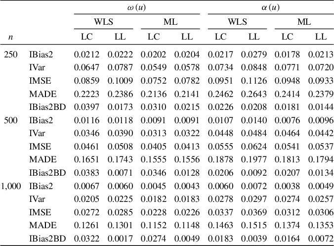
Table 1 Long description
The table is structured with two main parameter columns: omega of u and alpha of u. Under each parameter, there are two estimation methods: W L S and M L. Each method is further divided into L C (Local Constant) and L L (Local Linear) estimators.
Data is organized by sample size n:
* For n = 250:
- omega of u: I Bias 2 ranges from 0.0202 to 0.0222; I Var from 0.0549 to 0.0787; I M S E from 0.0752 to 0.1009; M A D E from 0.2136 to 0.2386.
- alpha of u: I Bias 2 ranges from 0.0178 to 0.0279; I Var from 0.0720 to 0.0848; I M S E from 0.0933 to 0.1126; M A D E from 0.2379 to 0.2643.
* For n = 500:
- omega of u: I Bias 2 ranges from 0.0091 to 0.0118; I Var from 0.0313 to 0.0390; I M S E from 0.0405 to 0.0508; M A D E from 0.1555 to 0.1743.
- alpha of u: I Bias 2 ranges from 0.0076 to 0.0140; I Var from 0.0442 to 0.0484; I M S E from 0.0537 to 0.0624; M A D E from 0.1794 to 0.1977.
* For n = 1,000:
- omega of u: I Bias 2 ranges from 0.0043 to 0.0067; I Var from 0.0182 to 0.0225; I M S E from 0.0226 to 0.0285; M A D E from 0.1148 to 0.1301.
- alpha of u: I Bias 2 ranges from 0.0038 to 0.0072; I Var from 0.0257 to 0.0297; I M S E from 0.0306 to 0.0369; M A D E from 0.1353 to 0.1515.
An additional metric, I Bias 2 B D, consistently shows lower values for L L compared to L C across all sample sizes and parameters.
To compare the performance of the estimators near the end of the sample, we also evaluate the bias of the estimators for the first and last 2.5% of time periods corresponding to
$u\in \left [ 0,0.025\right ] \cup \left [ 0.975,1 \right ] $
 . This is reported as IBias2BD in Table 1. As predicted by the theory, we find that, relative to the local constant versions, the local linear WLS and ML estimators enjoy significantly smaller biases near the boundaries of
$\left [ 0,1\right ] $
. This is reported as IBias2BD in Table 1. As predicted by the theory, we find that, relative to the local constant versions, the local linear WLS and ML estimators enjoy significantly smaller biases near the boundaries of
$\left [ 0,1\right ] $
 for all sample sizes.
5.2 Time-Varying Poisson Autoregression with Exogenous Covariates (PARX)
We here report simulation results for the local linear MLE of the following PARX(1) model with an additional exogenous regressor
$X_{n,t}$
 :
:

where
$\omega \left (u\right )=0.6-0.3u+0.3\sin \left (2\pi u\right )$
 ,
$ \alpha \left (u\right )=0.3+0.3u-0.3\sin \left (2\pi u\right )$
,
$ \alpha \left (u\right )=0.3+0.3u-0.3\sin \left (2\pi u\right )$
 , and
$ \gamma \left (u\right )=1-0.5\cos \left (\pi u\right )$
, and
$ \gamma \left (u\right )=1-0.5\cos \left (\pi u\right )$
 . The dynamics of the exogenous regressor was chosen as

where either
-
• DGP1: $\sigma \left (u\right )=0.8$
and
$\beta \left (u\right )=0.4$
so that
$X_{n,t}=X_{t}$
is strictly stationary. -
• DGP2: $\sigma \left (u\right )=0.8+0.4\cos \left (2\pi u\right )$
and
$ \beta \left (u\right )=0.4-0.2\sin \left (2\pi u\right )$
so
$X_{n,t}$
is locally stationary.





Table 2 reports the overall performance of the estimators in terms of integrated squared bias, variance, MSE, and MADE. The table shows that, in all sample sizes, the local linear estimator behaves well for both DGP1 and DGP2. All bias, variance, and MADE decrease as the sample size increases. Finally, similar to the case of the tvARCH model, the local linear estimator performs well near the boundaries; we leave out these results since they are similar to the ones reported for the tv-ARCH model above.
Performance of the local linear estimators for tvPARX models: Integrated squared bias (IBias2), integrated variance (IVar), integrated mean squared errors (IMSE), and median of MADE.
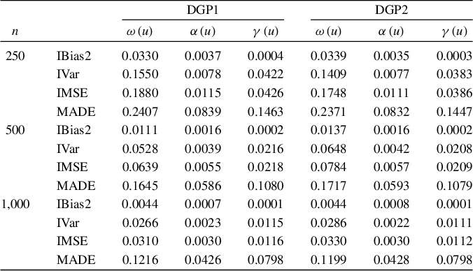
Table 2 Long description
The table compares performance metrics for parameters omega of u, alpha of u, and gamma of u across two data generating processes, D G P 1 and D G P 2. The metrics include I Bias 2, I Var, I M S E, and M A D E.
* For n = 250:
- D G P 1: omega of u has an I M S E of 0.1880; alpha of u is 0.0115; gamma of u is 0.0426.
- D G P 2: omega of u has an I M S E of 0.1748; alpha of u is 0.0111; gamma of u is 0.0386.
* For n = 500:
- D G P 1: omega of u has an I M S E of 0.0639; alpha of u is 0.0055; gamma of u is 0.0218.
- D G P 2: omega of u has an I M S E of 0.0784; alpha of u is 0.0057; gamma of u is 0.0209.
* For n = 1,000:
- D G P 1: omega of u has an I M S E of 0.0310; alpha of u is 0.0030; gamma of u is 0.0116.
- D G P 2: omega of u has an I M S E of 0.0330; alpha of u is 0.0030; gamma of u is 0.0112.
Across all parameters and both D G P s, I Bias 2, I Var, I M S E, and M A D E consistently decrease as the sample size n increases from 250 to 1,000.
6 EMPIRICAL APPLICATION
We here revisit the empirical analysis of U.S. corporate defaults carried out in Agosto et al. (Reference Agosto, Cavaliere, Kristensen and Rahbek2016) with the aim of examining whether there is evidence of structural instability in the time series. The data set consists of monthly number of bankruptcies among Moody’s rated industrial firms in the United States for the period 1982–2011 (
$n=360$
 observations), collected from Moody’s Credit Risk Calculator (CRC). Figure 1 shows the time series of default counts together with its sample autocorrelation function, which reveals high temporal dependence in default counts and existence of default clusters over time.
Left: Number of defaults per month among Moody’s rated U.S. industrial firms in the period 1982–2011; Right: autocorrelation function of defaults.
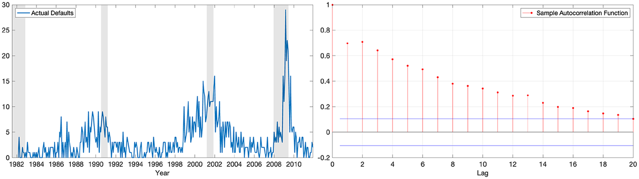
Figure 1 Long description
The left panel is a line graph titled Actual Defaults. The horizontal x-axis represents Year from 1982 to 2011. The vertical y-axis ranges from 0 to 30. The blue line shows fluctuating default counts with significant peaks around 1990, 2001, and a major spike reaching nearly 30 around 2009. Four vertical gray shaded regions highlight specific periods of high default activity.
The right panel is a stem plot titled Sample Autocorrelation Function. The horizontal x-axis represents Lag from 0 to 20. The vertical y-axis ranges from -0.2 to 1. Red dots on vertical stems show the correlation values. At lag 0, the value is 1. The correlation decreases steadily in a non-linear decay as the lag increases, reaching approximately 0.1 at lag 20. Two horizontal blue lines indicate the significance thresholds around the 0.1 and -0.1 marks on the y-axis.
With
$Y_{n,t}\in \left \{ 0,1,2,\ldots \right \} $
 ,
$t\geq 1$
,
$t\geq 1$
 denoting the number of defaults in a given month, we use a log-PARX model to gain better understanding of the dynamics of
$Y_{n,t}$
denoting the number of defaults in a given month, we use a log-PARX model to gain better understanding of the dynamics of
$Y_{n,t}$
 as a function of its own past,
$ Y_{n,t-m}$
as a function of its own past,
$ Y_{n,t-m}$
 ,
$m\geq 1$
,
$m\geq 1$
 , but also in terms of additional covariates
$ X_{n,t}\in \mathbb {R}^{d_{x}}$
, but also in terms of additional covariates
$ X_{n,t}\in \mathbb {R}^{d_{x}}$
 , which include relevant macroeconomic and financial factors as considered in Agosto et al. (Reference Agosto, Cavaliere, Kristensen and Rahbek2016). We model
$Y_{n,t}$
, which include relevant macroeconomic and financial factors as considered in Agosto et al. (Reference Agosto, Cavaliere, Kristensen and Rahbek2016). We model
$Y_{n,t}$
 as a conditional Poisson distribution
$Y_{n,t}|\mathcal {F}_{n,t-1}\sim \mathrm { Poisson}\left ( \lambda _{n,t}\left ( \theta \left ( t/n\right ) \right ) \right ) $
as a conditional Poisson distribution
$Y_{n,t}|\mathcal {F}_{n,t-1}\sim \mathrm { Poisson}\left ( \lambda _{n,t}\left ( \theta \left ( t/n\right ) \right ) \right ) $
 ,
$t=1,2,\ldots ,n$
,
$t=1,2,\ldots ,n$
 , where the intensity
$\lambda _{n,t}\left ( \theta \left ( t/n\right ) \right ) $
, where the intensity
$\lambda _{n,t}\left ( \theta \left ( t/n\right ) \right ) $
 depends on past counts, covariates
$X_{n,t-1}$
depends on past counts, covariates
$X_{n,t-1}$
 . and a vector of time-varying parameters
$\theta \left ( t/n\right ) $
. and a vector of time-varying parameters
$\theta \left ( t/n\right ) $
 . Our favored specification of
$\lambda _{n,t}\left ( \theta \right ) $
. Our favored specification of
$\lambda _{n,t}\left ( \theta \right ) $
 is the log-PARX model of Fokianos and Tjøstheim (Reference Fokianos and Tjøstheim2011), which is here augmented by the chosen set of exogenous variables,
$X_{n,t-1}$
is the log-PARX model of Fokianos and Tjøstheim (Reference Fokianos and Tjøstheim2011), which is here augmented by the chosen set of exogenous variables,
$X_{n,t-1}$
 ,
,

so that
$\theta =\left ( \omega ,\alpha _{1},\ldots ,\alpha _{p},\gamma ^{\prime }\right ) ^{\prime }$
 .
.
We here deviate from Agosto et al. (Reference Agosto, Cavaliere, Kristensen and Rahbek2016) that specifies
$\lambda _{n,t}$
 to be a linear function of past counts and factors. The reasons for us favoring the above log-specification over the linear one are three-fold: First, (25) do not impose positivity constraints on the parameters which facilitates the numerical computation of the estimators; second, it allows us to include any predictors we wish without the need of first transforming them to ensure that each component of the resulting
$X_{n,t-1}$
to be a linear function of past counts and factors. The reasons for us favoring the above log-specification over the linear one are three-fold: First, (25) do not impose positivity constraints on the parameters which facilitates the numerical computation of the estimators; second, it allows us to include any predictors we wish without the need of first transforming them to ensure that each component of the resulting
$X_{n,t-1}$
 is positive; third, when we estimate both models using the U.S. default data, we found that the log-specification delivers a better fit.
Similar to Agosto et al. (Reference Agosto, Cavaliere, Kristensen and Rahbek2016), we use
$\sum _{i=1}^{p}\alpha _{i}\left ( t/n\right ) $
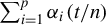 as a measure of contagion in the financial markets: If
$ \sum _{i=1}^{p}\alpha _{i}\left ( t/n\right ) $
as a measure of contagion in the financial markets: If
$ \sum _{i=1}^{p}\alpha _{i}\left ( t/n\right ) $
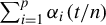 is large, then firms defaulting today will lead to a large increase in the risk of other firms defaulting next period everything else equal.
As exogenous covariates, we consider the same financial, credit market, and macroeconomic variables as in Agosto et al. (Reference Agosto, Cavaliere, Kristensen and Rahbek2016): Realized volatility (
$RV$
 ) computed using daily squared return on the S&P 500 index, the Leading Index released by the Federal Reserve (
$LI$
) computed using daily squared return on the S&P 500 index, the Leading Index released by the Federal Reserve (
$LI$
 ), year-to-year change in Industrial Production Index (
$IP$
), year-to-year change in Industrial Production Index (
$IP$
 ), one-year return on the S&P 500 index (
$SPX$
), one-year return on the S&P 500 index (
$SPX$
 ), the three-month Treasury bill rate (
$TB3$
), the three-month Treasury bill rate (
$TB3$
 ), and BAA Moody’s rated to 10-year Treasury spread (
$SP$
), and BAA Moody’s rated to 10-year Treasury spread (
$SP$
 ).Footnote
2
Agosto et al. (Reference Agosto, Cavaliere, Kristensen and Rahbek2016) decompose
$LI$
).Footnote
2
Agosto et al. (Reference Agosto, Cavaliere, Kristensen and Rahbek2016) decompose
$LI$
 and
$IP$
and
$IP$
 into their positive and negative parts to deal with above-mentioned issue of
$X_{n,t-1}$
into their positive and negative parts to deal with above-mentioned issue of
$X_{n,t-1}$
 having to be positive in the linear specification. In contrast, no such transformations are needed for our log-specification. Moreover, as well as
$RV$
having to be positive in the linear specification. In contrast, no such transformations are needed for our log-specification. Moreover, as well as
$RV$
 , we also consider the logarithm of
$RV$
, we also consider the logarithm of
$RV$
 ,
$\log \left ( RV\right ) $
,
$\log \left ( RV\right ) $
 , to evaluate if the latter is a better predictor; again, this would not be possible in the linear specification of Agosto et al. (Reference Agosto, Cavaliere, Kristensen and Rahbek2016).
The lag length p is chosen using BIC where, for a given model, the log-likelihood is evaluated at the estimated time-varying parameters.Footnote
3
According to this version of BIC, the preferred specification is
$p=2$
 . Importantly, by allowing for the parameters to be time-varying, a much more parsimonious model is selected by BIC: If we do model selection where for each model we restrict the estimated parameters to be constant over time, the preferred model is
$p=6$
. Importantly, by allowing for the parameters to be time-varying, a much more parsimonious model is selected by BIC: If we do model selection where for each model we restrict the estimated parameters to be constant over time, the preferred model is
$p=6$
 . Moreover, the persistence, or contagion, of the estimated time-invariant version, as measured by
$\sum _{i=1}^{p}\hat {\alpha }_{i}$
. Moreover, the persistence, or contagion, of the estimated time-invariant version, as measured by
$\sum _{i=1}^{p}\hat {\alpha }_{i}$
 , is substantially higher than for the time-varying version, as measured by
$\sum _{i=1}^{p}\hat {\alpha } _{i}\left ( u\right ) $
, is substantially higher than for the time-varying version, as measured by
$\sum _{i=1}^{p}\hat {\alpha } _{i}\left ( u\right ) $
 ,
$u\in \left [ 0,1\right ] $
,
$u\in \left [ 0,1\right ] $
 . This is consistent with the findings reported in Hillebrand (Reference Hillebrand2005) for GARCH models: Neglecting structural changes in parameters causes the estimates of these to be suffering from a strong upward bias which in turn leads BIC to selecting a bigger model.
As benchmark, we first estimate the time-invariant version of (25) with
$p=2$
 . Table 3 shows the estimation results for four different specifications of the time-invariant LLPARX(2) model: Column (1) contains the results when only
$\left ( RV,LI\right ) $
. Table 3 shows the estimation results for four different specifications of the time-invariant LLPARX(2) model: Column (1) contains the results when only
$\left ( RV,LI\right ) $
 are included; column (2) when only
$\left ( \log RV,LI\right ) $
are included; column (2) when only
$\left ( \log RV,LI\right ) $
 are included; column (3) when all covariates are included except for
$\log \left ( RV\right ) $
are included; column (3) when all covariates are included except for
$\log \left ( RV\right ) $
 ; and column (4) when all covariates except
$RV$
; and column (4) when all covariates except
$RV$
 are included. As in Agosto et al. (Reference Agosto, Cavaliere, Kristensen and Rahbek2016), once we control for the information contained in
$RV$
are included. As in Agosto et al. (Reference Agosto, Cavaliere, Kristensen and Rahbek2016), once we control for the information contained in
$RV$
 and
$LI$
and
$LI$
 , none of the other four covariates are found to be relevant in predicting future defaults. We also observe that the two specifications using
$\log \left ( RV\right ) $
, none of the other four covariates are found to be relevant in predicting future defaults. We also observe that the two specifications using
$\log \left ( RV\right ) $
 appear to perform better than the ones using
$RV$
appear to perform better than the ones using
$RV$
 . Based on these results, our favored specification of the time-varying version is to use
$LI$
. Based on these results, our favored specification of the time-varying version is to use
$LI$
 and
$\log \left ( RV\right ) $
and
$\log \left ( RV\right ) $
 as exogenous variables:

Estimation results of different LLPARX models.
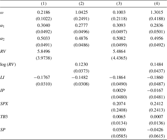
Table 3 Long description
The table consists of 5 columns (Parameter, Model 1, Model 2, Model 3, Model 4) and 10 parameter rows. Standard errors are provided in parentheses below each estimate.
* omega: Model 1 is 0.2186 (0.1022); Model 2 is 1.0425 (0.2491); Model 3 is 0.1003 (0.2118); Model 4 is 1.3015 (0.4188).
* alpha sub 1: Model 1 is 0.3040 (0.0492); Model 2 is 0.2777 (0.0496); Model 3 is 0.3093 (0.0497); Model 4 is 0.2836 (0.0501).
* alpha sub 2: Model 1 is 0.5033 (0.0491); Model 2 is 0.4876 (0.0486); Model 3 is 0.5082 (0.0499); Model 4 is 0.4956 (0.0492).
* R V: Model 1 is 5.8496 (3.9738); Model 3 is 5.4864 (4.4365). Models 2 and 4 are blank.
* log (R V): Model 2 is 0.1230 (0.0373); Model 4 is 0.1484 (0.0437). Models 1 and 3 are blank.
* L I: Model 1 is minus 0.1767 (0.0310); Model 2 is minus 0.1482 (0.0308); Model 3 is minus 0.1864 (0.0490); Model 4 is minus 0.1860 (0.0487).
* I P: Model 3 is 0.0029 (0.0480); Model 4 is minus 0.0167 (0.0481).
* S P W: Model 3 is 0.2074 (0.2408); Model 4 is 0.2412 (0.2413).
* R C 3: Model 3 is 0.0065 (0.0134); Model 4 is 0.0007 (0.0136).
* S Q: Model 3 is 0.0300 (0.0585); Model 4 is minus 0.0426 (0.0615).
Note: Standard errors are in parentheses.
Figure 2 shows the time series of the local linear estimates of the time-varying parameters of (26) together with the time-invariant estimates reported in column (2) of Table 3. Pointwise confidence bands are computed based on the asymptotic distribution derived in Theorem 3. The Leading Index is pointwise significant for most of the sample period which highlights the link between macroeconomic activity and corporate defaults also found in Agosto et al. (Reference Agosto, Cavaliere, Kristensen and Rahbek2016). At the same time, this link exhibits substantial time variation, in particular at the end of the sample during the Great Recession. The link between realized volatility and defaults of industrial firms is less significant but also appears to be changing over time. Similar to Agosto et al. (Reference Agosto, Cavaliere, Kristensen and Rahbek2016), the realized volatility and the Leading Index are strong explanatory variables during the Great Recession (2007–2011). However, differently, both of them are still relevant in the late 1980s and early 1990s. Especially, the effect of
$\log \left ( RV\right ) $
 tends to be negative in this period which cannot be captured by the aforementioned linear version of the PARX model.
Local linear estimate of time-varying parameter in eq. (26): Shaded areas are the 95% confidence intervals.
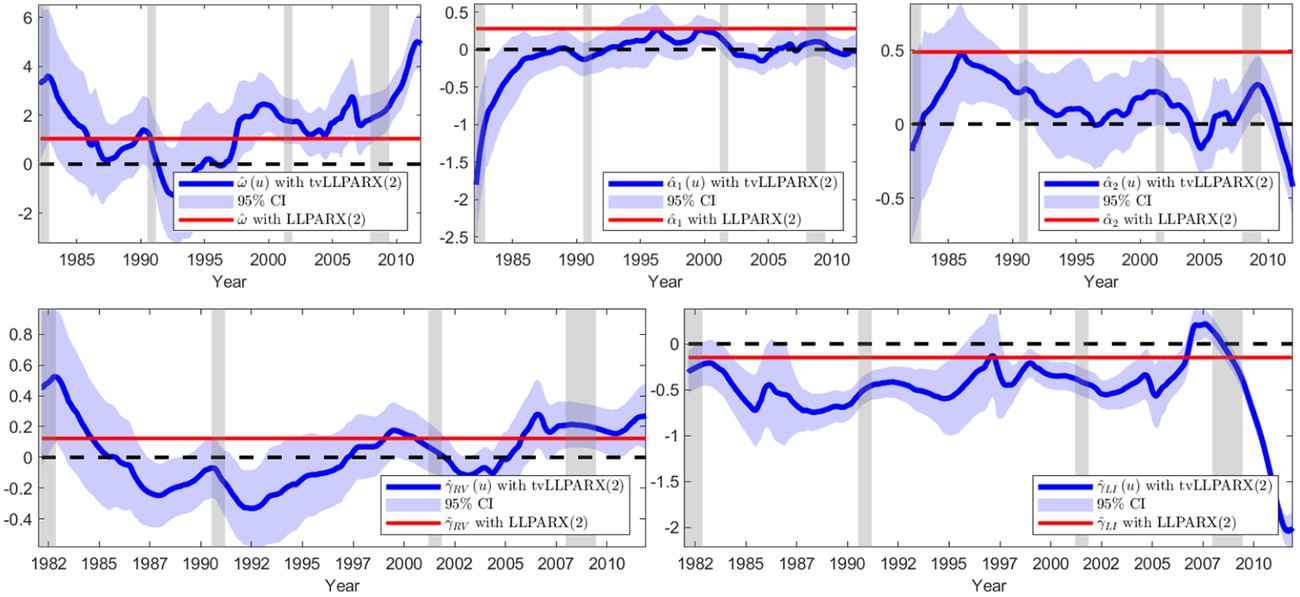
Figure 2 Long description
The figure consists of five panels arranged in two rows. Each panel plots a specific parameter estimate against the Year on the x-axis.
* Top-Left Panel: Plots omega hat (u) with tv L L P A R X (2). The y-axis ranges from minus 2 to 6. A blue line fluctuates significantly, starting near 4, dipping below 0 around 1992, and rising to 5 by 2012. A light blue shaded area represents the 95% C I. A horizontal red line sits at approximately 1.0.
* Top-Middle Panel: Plots alpha hat sub 1 (u). The y-axis ranges from minus 2.5 to 0.5. The blue line starts at minus 1.8 in 1982, rises to near 0 by 1990, and fluctuates slightly below the 0 dashed line until 2012. The red line is constant at 0.3.
* Top-Right Panel: Plots alpha hat sub 2 (u). The y-axis ranges from minus 0.5 to 0.5. The blue line peaks at 0.5 around 1986 and then trends downward with fluctuations toward minus 0.3. The red line is constant at 0.5.
* Bottom-Left Panel: Plots gamma hat sub R V (u). The y-axis ranges from minus 0.4 to 0.8. The blue line shows a wave-like pattern, dipping to minus 0.2 in 1992 and rising to 0.3 by 2012. The red line is constant at 0.1.
* Bottom-Right Panel: Plots gamma hat sub L I (u). The y-axis ranges from minus 2 to 0. The blue line stays between minus 0.5 and 0 until 2007, where it peaks slightly above 0 before sharply dropping to minus 2.0 by 2012. The red line is constant at minus 0.2.
All panels feature vertical grey shaded bars indicating specific time intervals and a dashed black horizontal line at y equals 0.
Finally, judging from
$\hat {\alpha }_{1}\left ( t/n\right ) +\hat {\alpha } _{2}\left ( t/n\right ) $
 , there is very little contagion in the financial markets from the 1990s onward, which is somewhat consistent with the findings in Agosto et al. (Reference Agosto, Cavaliere, Kristensen and Rahbek2016). However, at the end of the sample, we actually find a negative effect of today’s log-defaults on tomorrow’s default risk. Also note that the time-varying estimates,
$\hat {\alpha } _{1}\left ( t/n\right ) $
, there is very little contagion in the financial markets from the 1990s onward, which is somewhat consistent with the findings in Agosto et al. (Reference Agosto, Cavaliere, Kristensen and Rahbek2016). However, at the end of the sample, we actually find a negative effect of today’s log-defaults on tomorrow’s default risk. Also note that the time-varying estimates,
$\hat {\alpha } _{1}\left ( t/n\right ) $
 and
$\hat {\alpha }_{2}\left ( t/n\right ) $
and
$\hat {\alpha }_{2}\left ( t/n\right ) $
 , remain below the corresponding time-invariant ones,
$\hat {\alpha }_{1}$
, remain below the corresponding time-invariant ones,
$\hat {\alpha }_{1}$
 and
$\hat { \alpha }_{2}$
and
$\hat { \alpha }_{2}$
 as marked by the horizontal red lines, throughout the sample period. Again, this seems to indicate that ignoring time variation in the parameters of PARX models lead to over estimation of the level of persistence/contagion.
To assess in-sample fit and whether the reported time variation in the parameters is statistically significant, we carry out an array of graphical and quantitative diagnostic tools for time series. First, we plot in the left panel of Figure 3 the actual default counts together with the predicted defaults
$\hat {Y}_{n,t}:=\hat {\lambda } _{n,t}=\lambda _{n,t}\left ( \hat {\theta }\left ( t/n\right ) \right ) $
 . As can be seen from this plot, the time-varying LLPARX model captures the default counts dynamics well. In the right panel of Figure 3, the sample autocorrelation function of the standardized Pearson residuals
$ \hat {e}_{n,t}=\hat {\lambda }_{n,t}^{-1/2}\left ( Y_{n,t}-\hat {\lambda } _{n,t}\right ) $
. As can be seen from this plot, the time-varying LLPARX model captures the default counts dynamics well. In the right panel of Figure 3, the sample autocorrelation function of the standardized Pearson residuals
$ \hat {e}_{n,t}=\hat {\lambda }_{n,t}^{-1/2}\left ( Y_{n,t}-\hat {\lambda } _{n,t}\right ) $
 is plotted. Under correct specification,
$e_{n,t}$
is plotted. Under correct specification,
$e_{n,t}$
 should be white noise—the plotted sample autocorrelation function supports this.
Left: Actual number of defaults (blue) and estimated intensity (red); Right: Sample autocorrelation function of Pearson residuals.
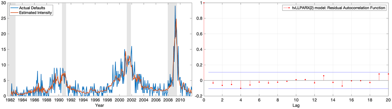
Figure 3 Long description
The figure consists of two panels arranged horizontally.
Left Panel: A line graph showing the time series of defaults from 1982 to 2012.
* The X axis is labeled Year, ranging from 1982 to 2012.
* The Y axis represents the count, ranging from 0 to 30.
* A blue line represents Actual Defaults, showing a highly volatile path with major peaks around 1991, 2002, and a primary spike exceeding 25 in 2009.
* A red line represents Estimated Intensity, which follows the blue line closely but with a smoother, less volatile trajectory.
* Four vertical grey shaded regions highlight specific periods of high default activity around 1982, 1991, 2001 to 2002, and 2008 to 2009.
Right Panel: A stem plot showing the sample A C F of Pearson residuals.
* The X axis is labeled Lag, ranging from 0 to 20.
* The Y axis ranges from minus 0.2 to 1.0.
* A legend at the top right identifies the data as t v L L P A R X 2 model Residual Autocorrelation Function.
* At Lag 0, the autocorrelation is exactly 1.0.
* For Lags 1 through 20, the red dots (stems) fluctuate near the zero line, almost entirely contained within the blue horizontal significance bounds located at approximately plus or minus 0.1.
We also evaluate the adequacy of fit using the probability integral transform (PIT). We follow Davis and Liu (Reference Davis and Liu2016) and compute the PITs by

where
$\left \{ \nu _{t}\right \} $
 is a sequence of i.i.d. random variables from a standard uniform distribution, and
$F_{n,t}$
is a sequence of i.i.d. random variables from a standard uniform distribution, and
$F_{n,t}$
 is the CDF of a Poisson(
$ \hat {\lambda }_{n,t})$
is the CDF of a Poisson(
$ \hat {\lambda }_{n,t})$
 distribution. Under correct model specification,
$\hat { u}_{n,t}$
distribution. Under correct model specification,
$\hat { u}_{n,t}$
 is a sequence of i.i.d. random variables from the standard uniform distribution. Figure 4 depicts the histogram of PIT which show that the tvLLPARX(2) model provides a better in-sample fit than the corresponding time-invariant model.
Left: Histograms of randomized PITs for log-linear PARX(2) and time-varying log-linear PARX(2) models fitted to the U.S. default data; Right: QQ-plots of the randomized PIT against standard uniform distribution for the corresponding models.
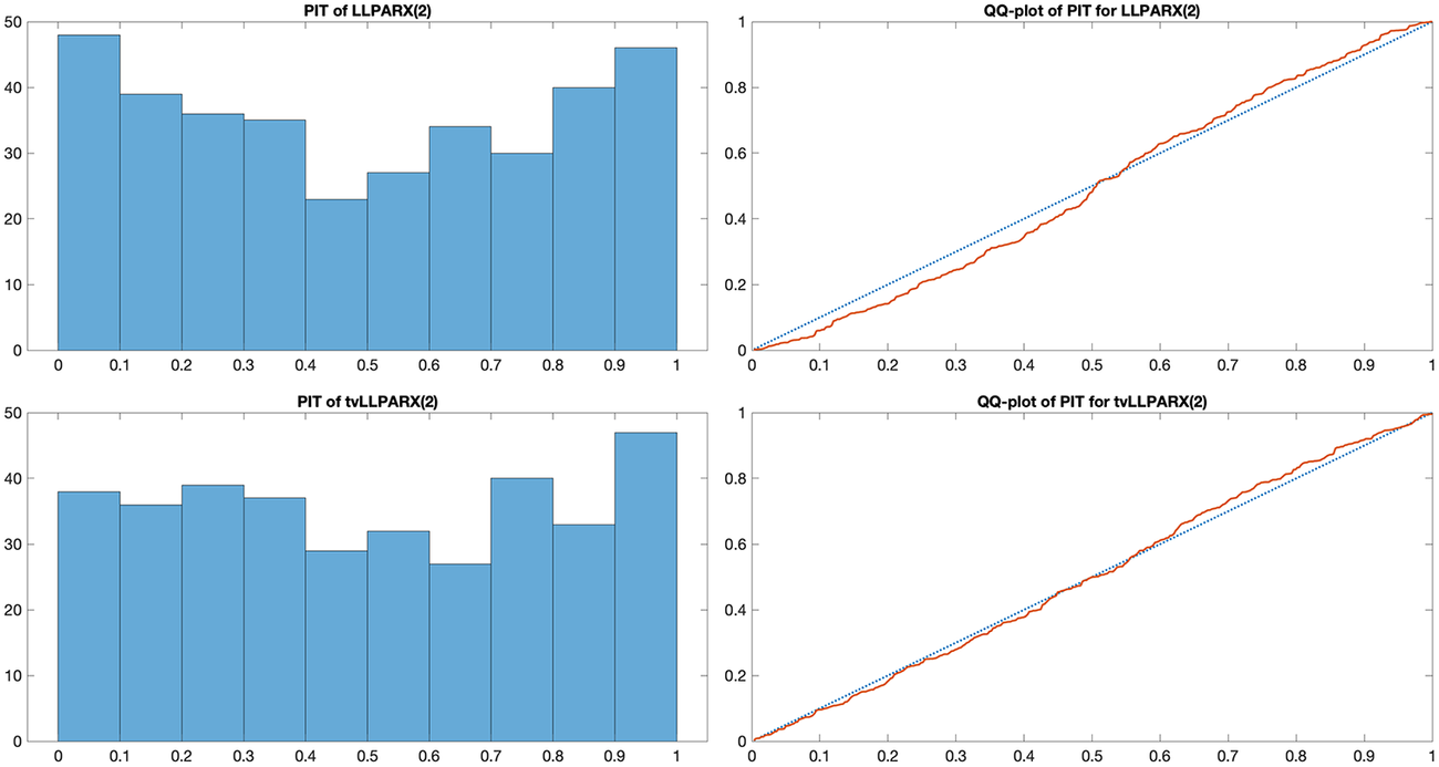
Figure 4 Long description
The figure consists of four panels arranged in a two-by-two grid.
Top-Left Panel: A histogram titled P I T of L L P A R X (2). The x-axis ranges from 0 to 1 in increments of 0.1, and the y-axis represents frequency from 0 to 50. The distribution is U-shaped, with the highest bars at the 0 to 0.1 and 0.9 to 1 intervals, and a trough in the center around 0.4 to 0.5.
Top-Right Panel: A Q Q plot titled Q Q-plot of P I T for L L P A R X (2). The x-axis and y-axis both range from 0 to 1. A blue dotted diagonal reference line represents a standard uniform distribution. An orange solid line representing the model data follows the diagonal but shows a slight S-shaped deviation, dipping below the line in the lower half and rising above it in the upper half.
Bottom-Left Panel: A histogram titled P I T of t v L L P A R X (2). The axes are identical to the top-left panel. The distribution is more uniform than the top-left, though it still shows a slight peak at the 0.9 to 1 interval and a minor dip between 0.4 and 0.7.
Bottom-Right Panel: A Q Q plot titled Q Q-plot of P I T for t v L L P A R X (2). The orange solid line follows the blue dotted diagonal reference line much more closely than the top-right plot, indicating a better fit to the standard uniform distribution.
Finally, in Table 4, we report the log-likelihood, AIC, and BIC values and the p-value from a Kolmogorov–Smirnov test of the PITs being uniformly distributed of each of four specifications in columns (1)–(4) of Table 3 together with the time-varying versions of (2) and (4), labeled tv (2) and tv(4), respectively. From these, we see that allowing for time-varying parameters increase the in-sample fit dramatically. While this is not a formal statistical test of time variation, it provides strong informal evidence of such. As mentioned earlier, we also see that specification (2) is favored over (1), (3), and (4) in the time-invariant case, and that (2) is favored over (4) in the time-varying case.
In-sample fit of time-invariant and time-varying LLPARX models.
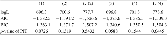
Table 4 Long description
The table consists of seven columns. The first column lists the metrics, while columns two through seven are labeled (1), (2), tv (2), (3), (4), and tv (4).
* Row 1, log L: (1) 696.3, (2) 700.6, tv (2) 777.7, (3) 696.8, (4) 701.8, tv (4) 778.6.
* Row 2, A I C: (1) minus 1,382.5, (2) minus 1,391.2, tv (2) minus 1,526.6, (3) minus 1,375.6, (4) minus 1,385.5, tv (4) minus 1,539.3.
* Row 3, B I C: (1) minus 1,363.1, (2) minus 1,371.7, tv (2) minus 1,507.2, (3) minus 1,340.6, (4) minus 1,350.5, tv (4) minus 1,504.3.
* Row 4, p-value of P I T: (1) 0.0726, (2) 0.1319, tv (2) 0.5432, (3) 0.0588, (4) 0.1544, tv (4) 0.6445.
We complete the analysis by conducting a final sensitivity analysis of (26). This is done by including the remaining exogenous covariates in addition to realized volatility and Leading Index in the time-varying version of the model:

The estimation results are provided in Figure 5. The estimates, except for the realized volatility, are consistent with our baseline findings. The Leading Index remains highly significant, which shows that macroeconomic factors are relevant in predicting future defaults. The link between short-term interest rates and defaults of industrial firms changes over time. During the late 1980s and the Great Recession (2007–2011), interest rates play a role in determining the interest expense of firms. In the 1990s, similar to the finding in Duffie et al. (Reference Duffie, Saita and Wang2007), the sign of the coefficient for the short-term rate is consistent with the fact that the U.S. Federal Reserve often increases the short-term rates to control business expansions. Controlling for
$LI$
 and
$TB3$
and
$TB3$
 , other covariates are estimated to be insignificant for most of the sample period except for the period of the Great Recession (2007–2011), in which financial, credit market, and macroeconomic variables are significant explanators of the default intensity. These are novel findings that the original analysis of Agosto et al. (Reference Agosto, Cavaliere, Kristensen and Rahbek2016) did not reveal.
Local linear estimate of time-varying parameter in eq. (27): Shaded areas are the 95% confidence intervals.
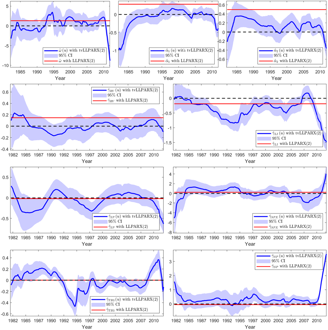
Figure 5 Long description
The figure consists of nine panels arranged in three rows and three columns. Each panel features a horizontal x-axis representing Year, ranging from approximately 1982 to 2010. The y-axis represents various parameter estimates. Each graph contains three main elements: a fluctuating blue line representing the time-varying local linear estimate (t v L L P A R X 2), a light blue shaded region representing the 95 percent confidence interval (C I), and a solid horizontal red line representing the constant estimate (L L P A R X 2). A dashed black line at zero serves as a baseline.
* Top-left panel: Parameter omega hat (u). The blue line fluctuates around the red line, which is set near 2.
* Top-center panel: Parameter alpha hat sub 1 (u). The blue line starts low at -1 and rises toward the red line at 0.3.
* Top-right panel: Parameter alpha hat sub 2 (u). The blue line fluctuates between 0 and 0.4, while the red line is at 0.5.
* Middle-left panel: Parameter gamma hat sub R V (u). The blue line shows a downward trend from 0.2 to -0.1, while the red line is constant at 0.15.
* Middle-center panel: Parameter gamma hat sub L I (u). The blue line shows a significant decline from 0 to -1.5 after 2007, while the red line is at -0.2.
* Middle-right panel: Parameter gamma hat sub S P X (u). The blue line is relatively stable near 0 until a sharp spike to 4 in 2010, while the red line is at 0.2.
* Bottom-left panel: Parameter gamma hat sub I P (u). The blue line oscillates around the red line and zero baseline.
* Bottom-center panel: Parameter gamma hat sub T B 3 (u). The blue line shows high volatility with a sharp dip in 1995 and a spike in 2010.
* Bottom-right panel: Parameter gamma hat sub S P (u). The blue line remains near 0 for most of the period before a vertical spike to 3.5 at the end of the timeline.
7 CONCLUSION AND FUTURE WORK
We have here developed a general theory for kernel regression-type estimators of time-varying parameters and used this to provide primitive conditions for the estimators in Markov models. Another interesting application would be infinite memory models of the form

The local constant estimator of
$\theta \left ( u\right ) $
 was analyzed in Bardet et al. (Reference Bardet, Doukhan and Wintenberger2022) using techniques different from ours. Specifically, they provide primitive conditions under which
$Y_{n,t}$
was analyzed in Bardet et al. (Reference Bardet, Doukhan and Wintenberger2022) using techniques different from ours. Specifically, they provide primitive conditions under which
$Y_{n,t}$
 satisfies

where
$Y_{t}^{\ast }\left ( u\right ) $
 is the stationary solution to
$ Y_{t}^{\ast }\left ( u\right ) =G\left ( Y_{t-1}^{\ast }\left ( u\right ) ,Y_{t-2}^{\ast }\left ( u\right ) ,\dots ,\varepsilon _{t};]\right.\left. \theta \left ( u\right ) \right ) $
is the stationary solution to
$ Y_{t}^{\ast }\left ( u\right ) =G\left ( Y_{t-1}^{\ast }\left ( u\right ) ,Y_{t-2}^{\ast }\left ( u\right ) ,\dots ,\varepsilon _{t};]\right.\left. \theta \left ( u\right ) \right ) $
 . But this result unfortunately does not suffice for our theory since this requires
$Y_{n,t}$
. But this result unfortunately does not suffice for our theory since this requires
$Y_{n,t}$
 to satisfy our version of local stationarity as given in Definition 1. At the same time, Bardet et al. (Reference Bardet, Doukhan and Wintenberger2022) do provide primitive conditions for the assumptions on the stationary version of Corollary 3 to hold. Thus, under the high-level assumption that
$Y_{n,t}$
to satisfy our version of local stationarity as given in Definition 1. At the same time, Bardet et al. (Reference Bardet, Doukhan and Wintenberger2022) do provide primitive conditions for the assumptions on the stationary version of Corollary 3 to hold. Thus, under the high-level assumption that
$Y_{n,t}$
 satisfies our version of local stationarity, we can combine the results of Bardet et al. (Reference Bardet, Doukhan and Wintenberger2022) with our Corollary 3 to obtain a theory for local polynomial estimators of infinite memory models. Under this high-level condition, we are also able to provide a precise characterization of the leading bias term of their estimator, something which was missing in the analysis of Bardet et al. (Reference Bardet, Doukhan and Wintenberger2022). We leave it to future research to establish primitive conditions under which infinite memory models satisfy our Definition 1.
A Appendix
A.1 Auxiliary Results
In the following, assume that L satisfies: (i)
$L\left ( \cdot \right ) $
 has a compact support and (ii) for some
$\Lambda <\infty $
has a compact support and (ii) for some
$\Lambda <\infty $
 ,
$\left \vert L(v)-L(v^{\prime })\right \vert \leq \Lambda \left \vert v-v^{\prime }\right \vert $
,
$\left \vert L(v)-L(v^{\prime })\right \vert \leq \Lambda \left \vert v-v^{\prime }\right \vert $
 ,
$v,v^{\prime }\in \mathbb {R}$
,
$v,v^{\prime }\in \mathbb {R}$
 . We denote
$L_{b}\left ( \cdot \right ) :=L\left ( \cdot /b\right ) /b$
. We denote
$L_{b}\left ( \cdot \right ) :=L\left ( \cdot /b\right ) /b$
 .
.
Lemma A1. The following hold as
$b\rightarrow 0$
 and
$ nb\rightarrow \infty $
and
$ nb\rightarrow \infty $
 :
:
(i) Suppose
$\left \{ W_{n,t}\left ( \theta \right ) \right \} $
 is ULS
$\left ( p,r,\Theta \right ) $
is ULS
$\left ( p,r,\Theta \right ) $
 with its stationary approximation
$\left \{ W_{t}^{\ast }\left ( \theta |u\right ) \right \} $
with its stationary approximation
$\left \{ W_{t}^{\ast }\left ( \theta |u\right ) \right \} $
 being
$L_{p}$
being
$L_{p}$
 continuous for some
$p\geq 1,r>0,$
continuous for some
$p\geq 1,r>0,$
 and
$\Theta $
and
$\Theta $
 is compact. Then, with
$\mathcal {A}$
is compact. Then, with
$\mathcal {A}$
 defined in Assumption 2 and for any
$u\in (0,1)$
defined in Assumption 2 and for any
$u\in (0,1)$
 ,
,

(ii) Suppose
$\left \{ W_{n,t},\mathcal {F}_{n,t}\right \} $
 is an MGD array and LS
$\left ( p,r\right ) $
is an MGD array and LS
$\left ( p,r\right ) $
 for some
$p\geq 2$
for some
$p\geq 2$
 and
$r>0$
and
$r>0$
 with its stationary approximation
$W_{t}^{\ast }\left ( u\right ) $
with its stationary approximation
$W_{t}^{\ast }\left ( u\right ) $
 being
$L_{p}$
being
$L_{p}$
 -continuous. Then, for any
$u\in (0,1)$
-continuous. Then, for any
$u\in (0,1)$
 ,
,
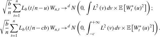
(iii) Suppose
$W_{t}^{\ast }\left ( u\right ) $
 is stationary and ergodic with
$\sum _{s=0}^{\infty }\left \vert \mathrm {Cov}\left ( W_{t}^{\ast }\left ( u\right ) ,W_{t+s}^{\ast }\left ( u\right ) \right ) \right \vert <\infty $
is stationary and ergodic with
$\sum _{s=0}^{\infty }\left \vert \mathrm {Cov}\left ( W_{t}^{\ast }\left ( u\right ) ,W_{t+s}^{\ast }\left ( u\right ) \right ) \right \vert <\infty $
 . Then,

Proof of (i)
We first show that for all
$\theta \in \Theta $
 ,
,

Note that
$L(v)=0$
 for
$\left \vert v\right \vert \geq \bar {v}$
for
$\left \vert v\right \vert \geq \bar {v}$
 for some
$\bar { v}>0$
for some
$\bar { v}>0$
 . Then, Minkowski’s inequality implies that
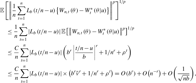
where we have used that

Next, with
$\bar {W}_{t}=W_{t}^{\ast }\left ( \theta |u\right ) -\mathbb {E} \left [ W_{t}^{\ast }\left ( \theta |u\right ) \right ] $
 ,
$\frac {1}{n} \sum _{t=1}^{n}L_{b}\left ( t/n-u\right ) \bar {W}_{t}=\frac {1}{nb}\sum _{t= \underline {t}}^{\bar {t}}L_{b}\left ( t/n-u\right ) \bar {W}_{t}$
,
$\frac {1}{n} \sum _{t=1}^{n}L_{b}\left ( t/n-u\right ) \bar {W}_{t}=\frac {1}{nb}\sum _{t= \underline {t}}^{\bar {t}}L_{b}\left ( t/n-u\right ) \bar {W}_{t}$
 for sufficiently large n, where
$\bar {t}=\left [ n\left ( u+\bar {v}b\right ) \right ] $
for sufficiently large n, where
$\bar {t}=\left [ n\left ( u+\bar {v}b\right ) \right ] $
 and
$\underline {t}=\left [ n\left ( u-\bar {v}b\right ) \right ] $
and
$\underline {t}=\left [ n\left ( u-\bar {v}b\right ) \right ] $
 . Here,
$\left [ x\right ] $
. Here,
$\left [ x\right ] $
 denotes the integer part of any real number x. By summation by parts, we have, with
$S_{n,t}=\sum _{j=\underline {t}}^{t}\bar { W_{j}}$
denotes the integer part of any real number x. By summation by parts, we have, with
$S_{n,t}=\sum _{j=\underline {t}}^{t}\bar { W_{j}}$
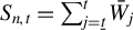 ,
,

Since
$\left \{ \bar {W}_{t}\right \} $
 is stationary,
$S_{n,t}$
is stationary,
$S_{n,t}$
 has the same distribution as
$\tilde {S}_{n,t}=\sum _{j=1}^{t-\underline {t}+1}\bar {W}_{j}$
has the same distribution as
$\tilde {S}_{n,t}=\sum _{j=1}^{t-\underline {t}+1}\bar {W}_{j}$
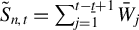 . Thus, for some constant M,
$\left \vert \frac {1}{n}\sum _{t=1}^{n}L_{b} \left ( t/n-u\right ) \bar {W}_{t}\right \vert \leq \frac {M}{nb}\sup _{t\leq \bar { t}-\underline {t}+1}\left \vert \tilde {S}_{n,t}\right \vert $
. Thus, for some constant M,
$\left \vert \frac {1}{n}\sum _{t=1}^{n}L_{b} \left ( t/n-u\right ) \bar {W}_{t}\right \vert \leq \frac {M}{nb}\sup _{t\leq \bar { t}-\underline {t}+1}\left \vert \tilde {S}_{n,t}\right \vert $
 . The ergodic theorem yields
$\tilde {S}_{n,t}/t\rightarrow 0$
. The ergodic theorem yields
$\tilde {S}_{n,t}/t\rightarrow 0$
 which in turn implies that
$ \frac {1}{n}\sum _{t=1}^{n}L_{b}\left ( t/n-u\right ) \bar {W}_{t}$
which in turn implies that
$ \frac {1}{n}\sum _{t=1}^{n}L_{b}\left ( t/n-u\right ) \bar {W}_{t}$
 tends to zero almost surely. Finally, using the mean-value theorem, there exists
$ v_{n,t}\in \left [ \frac {t-1}{n},\frac {t}{n}\right ] $
tends to zero almost surely. Finally, using the mean-value theorem, there exists
$ v_{n,t}\in \left [ \frac {t-1}{n},\frac {t}{n}\right ] $
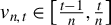 so that with
$\bar {L} =\sup _{v}\ L\left ( v\right ) $
so that with
$\bar {L} =\sup _{v}\ L\left ( v\right ) $
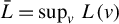 ,
,
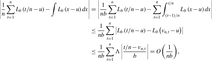
which shows that
$\frac {1}{n}\sum _{t=1}^{n}L_{b}\left ( t/n-u\right ) \mathbb {E }\left [ W_{t}^{\ast }\left ( \theta |u\right ) \right ] =\int L_{b}\left ( x-u\right ) dx\mathbb {E}\left [ W_{t}^{\ast }\left ( \theta |u\right ) \right ] +O\left ( 1/\left ( nb\right ) \right ) $
 .
.
For the uniform convergence, we note that by definition of
$\mathcal {A}$
 ,
$ D_{b}\left ( v-u\right ) \alpha \in \Theta $
,
$ D_{b}\left ( v-u\right ) \alpha \in \Theta $
 for all
$v\in \mathrm {supp}\left ( L\right ) $
for all
$v\in \mathrm {supp}\left ( L\right ) $
 and
$\alpha \in \mathcal {A}$
and
$\alpha \in \mathcal {A}$
 . Thus,
$\frac {1}{n} \sum _{t=1}^{n}K_{b}\left ( t/n-u\right ) W_{n,t}\left ( D_{n,t}\left ( u\right ) \alpha \right ) $
. Thus,
$\frac {1}{n} \sum _{t=1}^{n}K_{b}\left ( t/n-u\right ) W_{n,t}\left ( D_{n,t}\left ( u\right ) \alpha \right ) $
 , where
$D_{n,t}\left ( u\right ) =D_{b}\left ( t/n-u\right ) $
, where
$D_{n,t}\left ( u\right ) =D_{b}\left ( t/n-u\right ) $
 , is well-defined for
$\alpha \in \mathcal {A}$
, is well-defined for
$\alpha \in \mathcal {A}$
 , and
, and

Using Hölder’s and Minkowski’s inequalities,
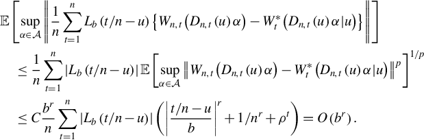
Next,
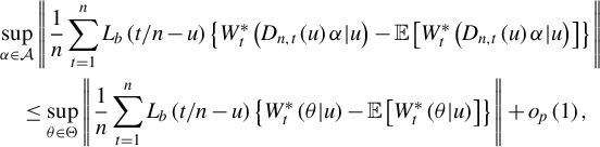
where
$\frac {1}{n}\sum _{t=1}^{n}L_{b}\left ( t/n-u\right ) \left \{ W_{t}^{\ast }\left ( \theta |u\right ) -\mathbb {E}\left [ W_{t}^{\ast }\left ( \theta |u\right ) \right ] \right \} =o_{P}\left ( 1\right ) $
 for all
$\theta \in \Theta $
for all
$\theta \in \Theta $
 . Thus, the result will follow if we can show stochastic equicontinuity of
$\theta \mapsto \frac {1}{n}\sum _{t=1}^{n}L_{b}\left ( t/n-u\right ) W_{t}^{\ast }\left ( \theta |u\right ) $
. Thus, the result will follow if we can show stochastic equicontinuity of
$\theta \mapsto \frac {1}{n}\sum _{t=1}^{n}L_{b}\left ( t/n-u\right ) W_{t}^{\ast }\left ( \theta |u\right ) $
 but this follows from the assumption of
$\theta \mapsto W_{t}^{\ast }\left ( \theta |u\right ) $
but this follows from the assumption of
$\theta \mapsto W_{t}^{\ast }\left ( \theta |u\right ) $
 being
$L_{p}$
being
$L_{p}$
 continuous: For a given
$\theta \in \Theta $
continuous: For a given
$\theta \in \Theta $
 and
$\epsilon>0,$
and
$\epsilon>0,$
 there exists
$\delta>0$
there exists
$\delta>0$
 so that
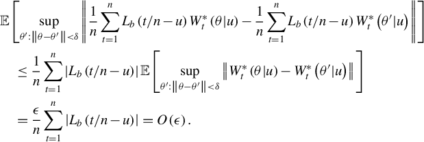
Proof of (ii). Observe that
$\sqrt {b/n}\sum _{t=1}^{n}L_{b}\left ( t/n-u\right ) W_{n,t}$
 is a martingale with quadratic variation
$Q_{n}=\frac {b }{n}\sum _{t=1}^{n}L_{b}^{2}\left ( t/n-u\right ) W_{n,t}^{2}$
is a martingale with quadratic variation
$Q_{n}=\frac {b }{n}\sum _{t=1}^{n}L_{b}^{2}\left ( t/n-u\right ) W_{n,t}^{2}$
 . Since
$W_{n,t}$
. Since
$W_{n,t}$
 is LS
$\left ( 2,r\right ) $
is LS
$\left ( 2,r\right ) $
 , it follows from part (i) that
$Q_{n}\rightarrow ^{p}\int L^{2}\left ( x\right ) dx\mathbb {E}\left [ W_{t}^{\ast }\left ( u\right ) ^{2}\right ] $
, it follows from part (i) that
$Q_{n}\rightarrow ^{p}\int L^{2}\left ( x\right ) dx\mathbb {E}\left [ W_{t}^{\ast }\left ( u\right ) ^{2}\right ] $
 . The result will then follow if the Lindeberg condition is satisfied (cf. Brown, Reference Brown1971). With
$m_{n,t}=\sqrt {b/n} L_{b}\left ( t/n-u\right ) W_{n,t}$
. The result will then follow if the Lindeberg condition is satisfied (cf. Brown, Reference Brown1971). With
$m_{n,t}=\sqrt {b/n} L_{b}\left ( t/n-u\right ) W_{n,t}$
 and
$m_{t}^{\ast }\left ( u\right ) =\sqrt { b/n}L_{b}\left ( t/n-u\right ) W_{t}^{\ast }\left ( u\right ) $
and
$m_{t}^{\ast }\left ( u\right ) =\sqrt { b/n}L_{b}\left ( t/n-u\right ) W_{t}^{\ast }\left ( u\right ) $
 ,
,
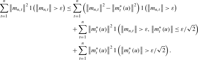
Recycling the arguments used in the proof of part (i), the first and third terms are
$o_{p}\left ( 1\right ) $
 . For the second term, employ the following inequality and Markov’s inequality:
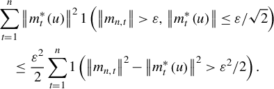
Proof of (iii). Assuming w.l.o.g. that
$\mathbb {E}\left [ W_{t}^{\ast }\right ] =0$
 ,
,

A.2 Proofs of Results in Section 3
Proof of Theorem 1
By Lemma A(i),
$\sup _{\alpha \in \mathcal {A}}\left \vert Q_{n}\left ( \alpha |u\right ) -Q^{\ast }\left ( \alpha |u\right ) \right \vert =o_{P}\left ( 1\right ) $
 , where
$Q^{\ast }\left ( \alpha |u\right ) =\int _{ \mathbb {R}}K\left ( v\right ) \mathbb {E}\left [ \ell _{t}^{\ast }\left ( D_{m}\left ( v\right ) \alpha |u\right ) \right ] dv$
, where
$Q^{\ast }\left ( \alpha |u\right ) =\int _{ \mathbb {R}}K\left ( v\right ) \mathbb {E}\left [ \ell _{t}^{\ast }\left ( D_{m}\left ( v\right ) \alpha |u\right ) \right ] dv$
 . Now, observe that for any
$\alpha =\left ( \alpha _{1},\ldots ,\alpha _{m+1}\right ) $
. Now, observe that for any
$\alpha =\left ( \alpha _{1},\ldots ,\alpha _{m+1}\right ) $
 with
$\alpha _{i}\neq 0$
with
$\alpha _{i}\neq 0$
 for some
$i\geq 2$
for some
$i\geq 2$
 , the polynomial
$v\mapsto D_{m}\left ( v\right ) \alpha $
, the polynomial
$v\mapsto D_{m}\left ( v\right ) \alpha $
 is non-constant almost everywhere. Thus, for any
$\alpha \neq \alpha ^{\ast }=\left ( \theta \left ( u\right ) ,0,\ldots ,0\right ) $
is non-constant almost everywhere. Thus, for any
$\alpha \neq \alpha ^{\ast }=\left ( \theta \left ( u\right ) ,0,\ldots ,0\right ) $
 ,
$D_{m}\left ( v\right ) \alpha \neq \theta \left ( u\right ) =D_{m}\left ( v\right ) \alpha ^{\ast }$
,
$D_{m}\left ( v\right ) \alpha \neq \theta \left ( u\right ) =D_{m}\left ( v\right ) \alpha ^{\ast }$
 for almost all
$v\in \left [ 0,1\right ] $
for almost all
$v\in \left [ 0,1\right ] $
 and so by Assumption 2(iii)
$\mathbb {E}\left [ \ell _{t}^{\ast }\left ( D_{m}\left ( v\right ) \alpha |u\right ) \right ] <\mathbb {E}\left [ \ell _{t}^{\ast }\left ( \theta \left ( u\right ) |u\right ) \right ] =\mathbb {E}\left [ \ell _{t}^{\ast }\left ( D_{m}\left ( v\right ) \alpha ^{\ast }|u\right ) \right ] $
and so by Assumption 2(iii)
$\mathbb {E}\left [ \ell _{t}^{\ast }\left ( D_{m}\left ( v\right ) \alpha |u\right ) \right ] <\mathbb {E}\left [ \ell _{t}^{\ast }\left ( \theta \left ( u\right ) |u\right ) \right ] =\mathbb {E}\left [ \ell _{t}^{\ast }\left ( D_{m}\left ( v\right ) \alpha ^{\ast }|u\right ) \right ] $
 for almost every v. Since
$K\left ( \cdot \right ) \geq 0,$
for almost every v. Since
$K\left ( \cdot \right ) \geq 0,$
 this in turn implies that
$ Q^{\ast }\left ( \alpha |u\right ) \leq Q^{\ast }\left ( \alpha ^{\ast }|u\right ) $
this in turn implies that
$ Q^{\ast }\left ( \alpha |u\right ) \leq Q^{\ast }\left ( \alpha ^{\ast }|u\right ) $
 . Finally, by the dominated convergence theorem together with Assumption 2(ii),
$\alpha \mapsto Q^{\ast }\left ( \alpha |u\right ) $
. Finally, by the dominated convergence theorem together with Assumption 2(ii),
$\alpha \mapsto Q^{\ast }\left ( \alpha |u\right ) $
 is continuous. This proves
$\hat {\alpha }\rightarrow ^{p}\alpha ^{\ast }$
is continuous. This proves
$\hat {\alpha }\rightarrow ^{p}\alpha ^{\ast }$
 (cf. Theorem 2.1 in Newey and McFadden, Reference Newey and McFadden1994).
Proof of Theorem 2
From Theorem 1, we know that
$\hat {\alpha }\rightarrow ^{p}\alpha ^{\ast }:=\left ( \theta \left ( u\right ) ,0,\dots ,0\right ) $
 . It is easily checked that the limit is situated in the interior of
$\mathcal {A}$
. It is easily checked that the limit is situated in the interior of
$\mathcal {A}$
 and so w.p.a.1. so will
$\hat {\alpha }$
and so w.p.a.1. so will
$\hat {\alpha }$
 . As a consequence,
$\hat {\alpha }$
. As a consequence,
$\hat {\alpha }$
 will satisfy (9) w.p.a.1. Adding and subtracting
$S_{n}\left ( u\right ) $
will satisfy (9) w.p.a.1. Adding and subtracting
$S_{n}\left ( u\right ) $
 and then rearranging yields

Here,
$H_{n}^{-1}\left ( \bar {\alpha }|u\right ) $
 is well-defined w.p.a.1 since, as shown below, it converges toward an invertible matrix. The claimed asymptotic result now follows if we can verify the claims of eqs. ( 13) and (14).
Proof of eq. (13). With
$L(u)=K(u)D_{m}\left ( u\right ) $
 ,
$\sqrt {nb}S_{n}\left ( u\right ) =\sqrt {\frac {b}{n}} \sum _{t=1}^{n}L_{b}(t/n-u)\otimes s_{n,t}$
,
$\sqrt {nb}S_{n}\left ( u\right ) =\sqrt {\frac {b}{n}} \sum _{t=1}^{n}L_{b}(t/n-u)\otimes s_{n,t}$
 . The result now follows from Lemma A(ii) under Assumption 4.
Proof of first claim of eq. (14). With
$ L(u)=K(u)D_{m}\left ( u\right ) D_{m}\left ( u\right ) ^{\prime }$
 , we can write
$H_{n}\left ( \beta |u\right ) =\frac {1}{n}\sum _{t=1}^{n}L_{b}(t/n-u)\otimes h_{n,t}\left ( D_{n,t}\left ( u\right ) \beta \right ) $
, we can write
$H_{n}\left ( \beta |u\right ) =\frac {1}{n}\sum _{t=1}^{n}L_{b}(t/n-u)\otimes h_{n,t}\left ( D_{n,t}\left ( u\right ) \beta \right ) $
 . It follows from Lemma A(i) and Assumption 5 that

where
$H\left (\theta |u\right )=\mathbb {E}\left [h_{t}^{*}\left (\theta |u\right ) \right ]$
 is continuous in
$\theta $
is continuous in
$\theta $
 and
$\mathcal {B}(\epsilon )=\{\alpha :\| \alpha -\alpha ^{*}\|<\epsilon \}$
and
$\mathcal {B}(\epsilon )=\{\alpha :\| \alpha -\alpha ^{*}\|<\epsilon \}$
 . Since
$\bar {\alpha }\to _p\alpha ^{*}$
. Since
$\bar {\alpha }\to _p\alpha ^{*}$
 and
$ D_m\left (v\right )\alpha ^{*}=\theta \left (u\right )$
and
$ D_m\left (v\right )\alpha ^{*}=\theta \left (u\right )$
 for all v, continuity of
$H(\cdot \mid u)$
for all v, continuity of
$H(\cdot \mid u)$
 yields

Finally,
$\mathbb {K}_{1}=\int K\left (v\right )D_{m}\left (v\right )D_{m}\left (v\right )^{\prime }dv$
 is positive definite under standard kernel conditions, and
$H(u)$
is positive definite under standard kernel conditions, and
$H(u)$
 is invertible by assumption.
Proof of second claim of eq. (14). First observe that
$D_{n,t}\left ( u\right ) \alpha ^{\ast }=\theta _{u}^{\ast }\left ( t/n\right ) $
 , where
$\theta _{u}^{\ast }\left ( t/n\right ) $
, where
$\theta _{u}^{\ast }\left ( t/n\right ) $
 was defined in eq. (1). Now, employ the mean-value theorem to obtain that, for some
$\bar {\theta }_{n,t}$
was defined in eq. (1). Now, employ the mean-value theorem to obtain that, for some
$\bar {\theta }_{n,t}$
 lying between
$\theta _{u}^{\ast }\left ( t/n\right ) $
lying between
$\theta _{u}^{\ast }\left ( t/n\right ) $
 and
$\theta \left ( t/n\right ) $
and
$\theta \left ( t/n\right ) $
 and some
$u_{n,t}\in \left [ t/n,u\right ] $
and some
$u_{n,t}\in \left [ t/n,u\right ] $
 ,
,
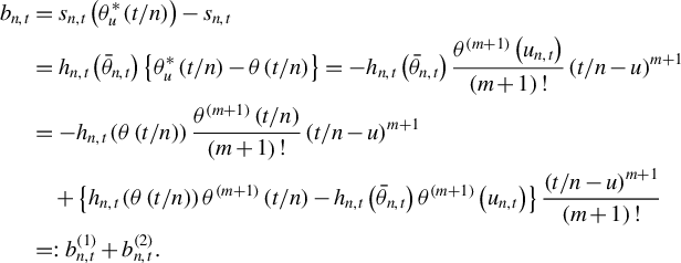
The first term is locally stationary and so by the same arguments as in the proof of Lemma A(ii):
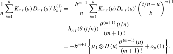
For the second term, observe that for
$\left \vert t/n-u\right \vert \leq Cb$
 ,
$\lVert \bar {\theta }_{n,t}-\theta \left ( t/n\right ) \rVert \leq \lVert \theta _{u}^{\ast }\left ( t/n\right ) -\theta \left ( t/n\right ) \rVert \leq \tilde {C}b^{m+1}$
,
$\lVert \bar {\theta }_{n,t}-\theta \left ( t/n\right ) \rVert \leq \lVert \theta _{u}^{\ast }\left ( t/n\right ) -\theta \left ( t/n\right ) \rVert \leq \tilde {C}b^{m+1}$
 , and so, using the ULS property of
$h_{n,t}\left ( \theta \right ) $
, and so, using the ULS property of
$h_{n,t}\left ( \theta \right ) $
 ,
,

as
$n\rightarrow \infty $
 and
$b\rightarrow 0$
and
$b\rightarrow 0$
 . Similarly,
$\sup _{n,t}\lVert \theta ^{\left ( m+1\right ) }\left ( t/n\right ) -\theta ^{\left ( m+1\right ) }\left ( u_{n,t}\right ) \rVert \rightarrow 0$
. Similarly,
$\sup _{n,t}\lVert \theta ^{\left ( m+1\right ) }\left ( t/n\right ) -\theta ^{\left ( m+1\right ) }\left ( u_{n,t}\right ) \rVert \rightarrow 0$
 as
$n\rightarrow \infty $
as
$n\rightarrow \infty $
 . These two results combined show that the
$\frac {b^{m+1}}{n} \sum _{t=1}^{n}K_{n,t}\left ( u\right ) D_{n,t}\left ( u\right ) ^{\prime }\left ( \frac {t/n-u}{b}\right ) ^{m+1}b_{n,t}^{\left ( 2\right ) }=o_{p}\left ( 1\right ) $
. These two results combined show that the
$\frac {b^{m+1}}{n} \sum _{t=1}^{n}K_{n,t}\left ( u\right ) D_{n,t}\left ( u\right ) ^{\prime }\left ( \frac {t/n-u}{b}\right ) ^{m+1}b_{n,t}^{\left ( 2\right ) }=o_{p}\left ( 1\right ) $
 .
.
Proof of Theorem 3
Write

The proof proceeds exactly as the one of Theorem 2 except that the first-order expansion of
$b_{n,t}$
 is replaced by a second-order expansion of
$s_{n,t}\left ( \theta \right ) $
is replaced by a second-order expansion of
$s_{n,t}\left ( \theta \right ) $
 w.r.t.
$\theta $
w.r.t.
$\theta $
 combined with

where
$u_{n,t}$
 lies between u and
$t/n$
lies between u and
$t/n$
 . This yields
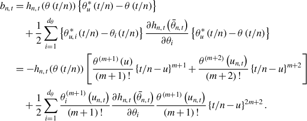
Thus, with
$L_{n,t}^{(m)}(u)=K_{n,t}\left ( u\right ) D_{n,t}\left ( u\right ) ^{\prime }\left ( \frac {t/n-u}{b}\right ) ^{m}$
 ,
,
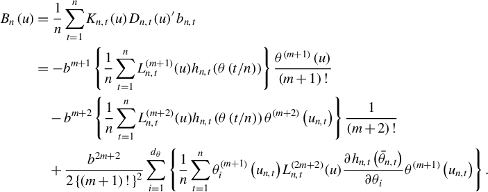
We now analyze the three bracketed terms. First,
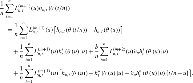
By Lemma A(iii) together with Assumption 8 and Lemma A(i),
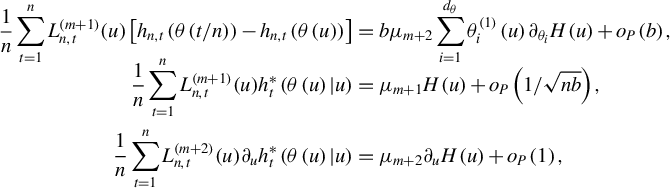
while, using Assumption 7, with
$h_{n,t}\left ( u\right ) =h_{n,t}\left ( \theta \left ( u\right ) \right ) $
 and
$h_{t}^{\ast }\left ( u\right ) =h_{t}^{\ast }\left ( \theta \left ( u\right ) |u\right ) $
and
$h_{t}^{\ast }\left ( u\right ) =h_{t}^{\ast }\left ( \theta \left ( u\right ) |u\right ) $
 ,
,
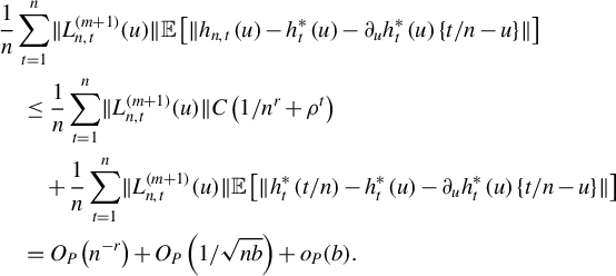
For the second and third terms, similar to the proof of eq. (14) and using Assumption 6,

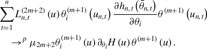
Collecting terms now yields the claimed result.
Proof of Corollary 1
The first part is a direct consequence of Theorem 3. To show the second part, first observe that

Next, using that
$\mathbb {E}\left [ s_{t}^{\ast }\left ( \theta \left ( v\right ) |v\right ) \right ] =0$
 for all v,

where it is easily checked that

Proof of Theorem 4
Inspecting the proof of Theorem 3, we observe that Assumptions 7 and 8 are only invoked in the analysis of
$\frac {1}{n} \sum _{t=1}^{n}L_{n,t}^{(m+1)}(u)h_{n,t}\left ( \theta \left ( t/n\right ) \right ) $
 . We here re-analyze this term under Assumptions 9 and 10: Write
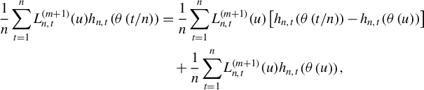
where the first term satisfies eq. (A.1). Now, with
$ h_{n,t}:=h_{n,t}\left ( \theta \left ( u\right ) \right ) $
 and
$h_{t}^{\ast }\left ( v\right ) :=h_{t}^{\ast }\left ( \theta \left ( u\right ) |v\right ) $
and
$h_{t}^{\ast }\left ( v\right ) :=h_{t}^{\ast }\left ( \theta \left ( u\right ) |v\right ) $
 ,
,
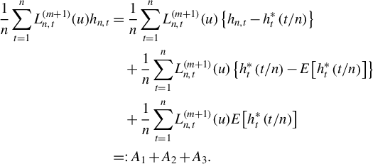
By Assumption 5(ii),

for any element
$A_{2,i,j}$
 of
$A_{2}$
of
$A_{2}$
 , by Assumption 10 and with
$V_{\left \vert t_{1}-t_{2}\right \vert }^{\left ( i,j\right ) }\left ( v_{1},v_{2}\right ) =$
, by Assumption 10 and with
$V_{\left \vert t_{1}-t_{2}\right \vert }^{\left ( i,j\right ) }\left ( v_{1},v_{2}\right ) =$
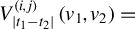 Cov
$\left ( h_{t_{1},i,j}^{\ast }\left ( v_{1}\right ) ,h_{t_{2},i,j}^{\ast }\left ( \theta \left ( v_{2}\right ) |u\right ) \right ) $
Cov
$\left ( h_{t_{1},i,j}^{\ast }\left ( v_{1}\right ) ,h_{t_{2},i,j}^{\ast }\left ( \theta \left ( v_{2}\right ) |u\right ) \right ) $
 ,
,
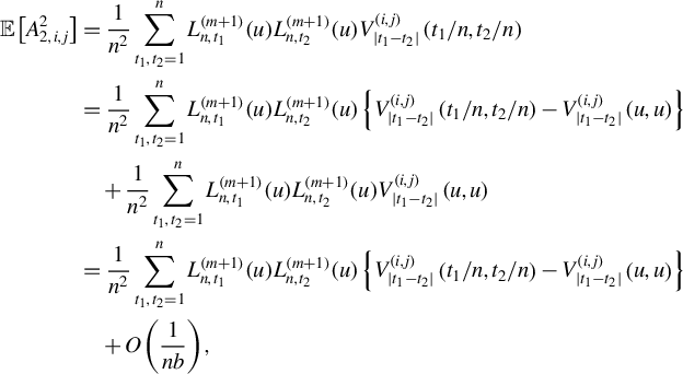
where, with

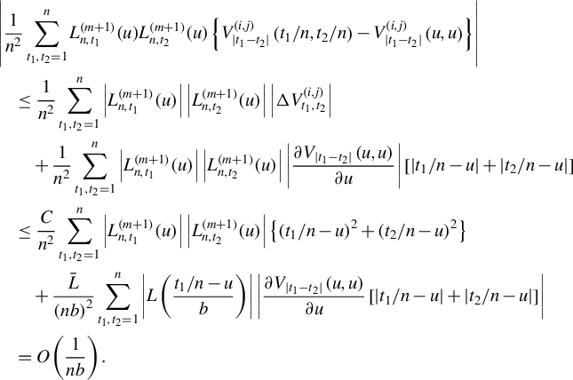
Finally, by Assumption 9,
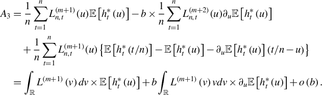
A.3 Proofs of Results in Section 4
Proof of Lemma 1
First, for any
$p>0$
 , with
$\lVert \mathcal {Z}_{n,t}\left ( \theta \right ) \rVert _{a,p}:=\left ( \sum _{i=1}^{\infty }a_{i}\lVert Z_{n,t+1-i}\left ( \theta \right ) \rVert ^{p}\right ) ^{1/p}$
, with
$\lVert \mathcal {Z}_{n,t}\left ( \theta \right ) \rVert _{a,p}:=\left ( \sum _{i=1}^{\infty }a_{i}\lVert Z_{n,t+1-i}\left ( \theta \right ) \rVert ^{p}\right ) ^{1/p}$
 ,
,
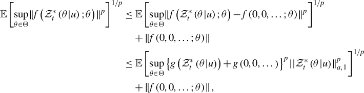
where, for any
$q_{1},q_{2}$
 satisfying
$1/q_{1}+1/q_{2}=1$
satisfying
$1/q_{1}+1/q_{2}=1$
 ,
,
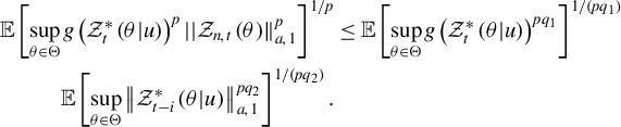
For the right-hand side to be finite, we need
$pq_{1}=p_{2}$
 ,
$pq_{2}=p_{1}$
,
$pq_{2}=p_{1}$
 and
$1/q_{1}+1/q_{2}=1$
and
$1/q_{1}+1/q_{2}=1$
 ; that is,
$q_{1}=p_{2}/p$
; that is,
$q_{1}=p_{2}/p$
 and
$q_{2}=p_{1}/p$
and
$q_{2}=p_{1}/p$
 and
$ 1/q_{1}+1/q_{2}=p\left \{ 1/p_{1}+1/p_{2}\right \} =1\Leftrightarrow p=\left \{ 1/p_{1}+1/p_{2}\right \} ^{-1}$
and
$ 1/q_{1}+1/q_{2}=p\left \{ 1/p_{1}+1/p_{2}\right \} =1\Leftrightarrow p=\left \{ 1/p_{1}+1/p_{2}\right \} ^{-1}$
 . Thus,
$f\left ( \mathcal {Z}_{t}^{\ast }\left ( \theta |u\right ) ;\theta \right ) $
. Thus,
$f\left ( \mathcal {Z}_{t}^{\ast }\left ( \theta |u\right ) ;\theta \right ) $
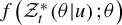 is well-defined in the
$L_{p}$
is well-defined in the
$L_{p}$
 -sense. With our choices of
$q_{1}$
-sense. With our choices of
$q_{1}$
 ,
$q_{2}$
,
$q_{2}$
 , and p,
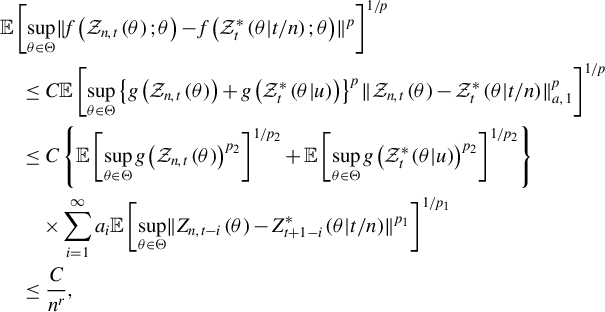
and, similarly,
$\mathbb {E}\left [ \sup _{\theta \in \Theta }\lVert f\left ( \mathcal {Z}_{t}^{\ast }\left ( \theta |u\right ) ;\theta \right ) -f\left ( \mathcal {Z}_{t}^{\ast }\left ( \theta |v\right ) ;\theta \right ) \rVert ^{p} \right ] ^{1/p}\leq C\left \vert u-v\right \vert {}^{r} $
 .
.
Under (ii’) and (iii’), condition (ii) of the first part of the lemma is satisfied with
$p_{2}=p_{1}/s\geq 1$
 :
:
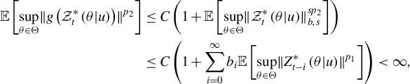
and similarly for
$\mathbb {E}\left [ \sup _{\theta \in \Theta }\lVert g\left ( \mathcal {Z}_{n,t}\left ( \theta \right ) \right ) \rVert ^{p_{2}}\right ] $
 . Thus, the conclusions of the first part hold with
$p=\left ( 1/p_{1}+1/\left ( p_{1}/s\right ) \right ) ^{-1}=p_{1}/\left ( s+1\right ) $
. Thus, the conclusions of the first part hold with
$p=\left ( 1/p_{1}+1/\left ( p_{1}/s\right ) \right ) ^{-1}=p_{1}/\left ( s+1\right ) $
 .
.
To show the third part, let
$\tilde {Z}_{t}^{\ast }\left ( \theta |u\right ) $
 be an independent copy of
$Z_{t}^{\ast }\left ( \theta |u\right ) $
be an independent copy of
$Z_{t}^{\ast }\left ( \theta |u\right ) $
 . Applying the same inequalities as in the first part,

The claimed result now follows from the definition of
$\tau $
 -weak dependence (cf. p. 1999 of Doukhan and Wintenberger, Reference Doukhan and Wintenberger2008). This in turn implies that the short-memory condition is satisfied (cf. Doukhan and Wintenberger, Reference Doukhan and Wintenberger2008).
Before proving Lemma 3, first consider q-Markov models without covariates on the form

where
$G:\mathcal {Y}^{q}\times \mathcal {E}\times \Theta \mapsto \mathcal {Y}$
 is some known mapping,
$\varepsilon _{t}\in \mathcal {E}\subseteq \mathbb {R} ^{d_{\varepsilon }}$
is some known mapping,
$\varepsilon _{t}\in \mathcal {E}\subseteq \mathbb {R} ^{d_{\varepsilon }}$
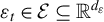 is a sequence of i.i.d. errors, and
$\theta \left ( \cdot \right ) \in \Theta $
is a sequence of i.i.d. errors, and
$\theta \left ( \cdot \right ) \in \Theta $
 . Importantly, the initial value
$Y_{n,0}$
. Importantly, the initial value
$Y_{n,0}$
 can be arbitrarily chosen which is in contrast to most of the existing literature. Under regularity conditions, its corresponding stationary approximation
$ Y_{t}^{\ast }\left ( u\right ) $
can be arbitrarily chosen which is in contrast to most of the existing literature. Under regularity conditions, its corresponding stationary approximation
$ Y_{t}^{\ast }\left ( u\right ) $
 will solve

We impose the following assumptions.
Assumption 13. (i)
$\sup _{\theta \in \Theta }\mathbb {E}\left [ \lVert G\left ( y_{0},\varepsilon _{t};\theta \right ) \rVert ^{p}\right ] <\infty $
 for some
$y_{0}\in \mathcal {Y}^{q}$
for some
$y_{0}\in \mathcal {Y}^{q}$
 and
$p>0$
and
$p>0$
 ; (ii) there exists
$\rho <1$
; (ii) there exists
$\rho <1$
 so that for all
$y,y^{\prime }\in \mathcal {Y}^{q}$
so that for all
$y,y^{\prime }\in \mathcal {Y}^{q}$
 ,
$\mathbb {E}\left [ \lVert G\left ( y,\varepsilon _{t};\theta \right ) -G\left ( y^{\prime },\varepsilon _{t};\theta \right ) \rVert ^{p}\right ] ^{1/p}\leq \rho \lVert y-y^{\prime }\rVert $
,
$\mathbb {E}\left [ \lVert G\left ( y,\varepsilon _{t};\theta \right ) -G\left ( y^{\prime },\varepsilon _{t};\theta \right ) \rVert ^{p}\right ] ^{1/p}\leq \rho \lVert y-y^{\prime }\rVert $
 ; (iii) there exist
$\tilde {p}\geq 1$
; (iii) there exist
$\tilde {p}\geq 1$
 ,
$r>0,$
,
$r>0,$
 and
$\delta \geq 0$
and
$\delta \geq 0$
 so that for all
$\theta ,\theta ^{\prime }\in \Theta $
so that for all
$\theta ,\theta ^{\prime }\in \Theta $
 ,
$\mathbb {E}\left [ \lVert G\left ( y,\varepsilon _{t};\theta \right ) -G\left ( y,\varepsilon _{t};\theta ^{\prime }\right ) \rVert ^{\tilde {p}}\right ] ^{1/\tilde {p}}\leq C\left ( 1+\lVert y\rVert ^{\delta }\right ) \lVert \theta -\theta ^{\prime }||^{r}$
,
$\mathbb {E}\left [ \lVert G\left ( y,\varepsilon _{t};\theta \right ) -G\left ( y,\varepsilon _{t};\theta ^{\prime }\right ) \rVert ^{\tilde {p}}\right ] ^{1/\tilde {p}}\leq C\left ( 1+\lVert y\rVert ^{\delta }\right ) \lVert \theta -\theta ^{\prime }||^{r}$
 ; and (iv)
$\mathbb {E}\left [ \lVert Y_{n,0}\rVert ^{\tilde {p}}\right ] <\infty $
; and (iv)
$\mathbb {E}\left [ \lVert Y_{n,0}\rVert ^{\tilde {p}}\right ] <\infty $
 and
$\mathbb {E}\left [ \lVert G\left ( y,\varepsilon _{t};\theta \right ) -G\left ( y,\varepsilon _{t};\theta ^{\prime }\right ) \rVert ^{\tilde { p}}\right ] ^{1/\tilde {p}}\leq C\left ( 1+\lVert y\rVert ^{\delta }\right ) \lVert \theta -\theta ^{\prime }||^{r}.$
and
$\mathbb {E}\left [ \lVert G\left ( y,\varepsilon _{t};\theta \right ) -G\left ( y,\varepsilon _{t};\theta ^{\prime }\right ) \rVert ^{\tilde { p}}\right ] ^{1/\tilde {p}}\leq C\left ( 1+\lVert y\rVert ^{\delta }\right ) \lVert \theta -\theta ^{\prime }||^{r}.$

Lemma 5. Under Assumption 13(i) and (ii), there exists a stationary and
$\tau $
 -weakly dependent solution,
$\left \{ Y_{t}^{\ast }\left ( u\right ) \right \} $
-weakly dependent solution,
$\left \{ Y_{t}^{\ast }\left ( u\right ) \right \} $
 to (A.2) with
$ \sup _{u\in \left [ 0,1\right ] }\mathbb {E}\left [ \lVert Y_{t}^{\ast }\left ( u\right ) \rVert ^{p}\right ] <\infty $
to (A.2) with
$ \sup _{u\in \left [ 0,1\right ] }\mathbb {E}\left [ \lVert Y_{t}^{\ast }\left ( u\right ) \rVert ^{p}\right ] <\infty $
 with
$\tau _{Y}\left ( k\right ) \leq O\left ( \rho ^{k}\right ) $
with
$\tau _{Y}\left ( k\right ) \leq O\left ( \rho ^{k}\right ) $
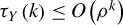 . If furthermore Assumption 13 (iii) and (iv) holds,
$\sup _{u\in \left [ 0,1\right ] }\mathbb {E}\left [ \lVert Y_{t}^{\ast }\left ( u\right ) \rVert ^{\tilde {p}\delta }\right ] <\infty $
. If furthermore Assumption 13 (iii) and (iv) holds,
$\sup _{u\in \left [ 0,1\right ] }\mathbb {E}\left [ \lVert Y_{t}^{\ast }\left ( u\right ) \rVert ^{\tilde {p}\delta }\right ] <\infty $
 and
$\theta \left ( \cdot \right ) \in \Theta $
and
$\theta \left ( \cdot \right ) \in \Theta $
 is continuously differentiable, then
$Y_{n,t}$
is continuously differentiable, then
$Y_{n,t}$
 is LS
$\left ( \tilde {p},r\right ) $
is LS
$\left ( \tilde {p},r\right ) $
 with
$\sup _{n,t}\mathbb {E} \left [ \lVert Y_{n,t}\rVert ^{\tilde {p}}\right ] <\infty $
with
$\sup _{n,t}\mathbb {E} \left [ \lVert Y_{n,t}\rVert ^{\tilde {p}}\right ] <\infty $
 for any given initial value
$Y_{n,0}$
for any given initial value
$Y_{n,0}$
 with
$\mathbb {E}\left [ \lVert Y_{n,0}\rVert ^{p}\right ] <\infty $
with
$\mathbb {E}\left [ \lVert Y_{n,0}\rVert ^{p}\right ] <\infty $
 .
.
Proof of Lemma 5
The first part of the result follows from Corollary 3.1 of Doukhan and Wintenberger (Reference Doukhan and Wintenberger2008).
For the second part, define the stacked state vectors

and define the associated Markov(1) update map
$F:\mathcal {Y}^{q}\times \mathcal {E}\times \Theta \to \mathcal {Y}^{q}$
 by
by

Then the q-Markov recursion is equivalent to the Markov(1) recursion on the enlarged state space:

Therefore, it suffices to prove the desired bounds for the Markov(1) process
$\{\mathbf {Y}_{n,t}\}$
 ; the corresponding bounds for
$Y_{n,t}$
; the corresponding bounds for
$Y_{n,t}$
 follow immediately since
$Y_{n,t}$
follow immediately since
$Y_{n,t}$
 is the first coordinate of
$\mathbf {Y}_{n,t}$
is the first coordinate of
$\mathbf {Y}_{n,t}$
 (and similarly for
$Y_t^*(u)$
(and similarly for
$Y_t^*(u)$
 ). In what follows, we write the argument for the Markov(1) recursion and apply it to
$\mathbf {Y}$
). In what follows, we write the argument for the Markov(1) recursion and apply it to
$\mathbf {Y}$
 .
.
For
$u,v\in [0,1]$
 , using the Markov(1) recursion and the triangle inequality,
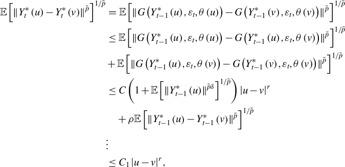
where
$C_{1}=C\left ( 1+\sup _{u\in \left [ 0,1\right ] }\mathbb {E}\left [ \lVert Y_{t-1}^{\ast }\left ( u\right ) \rVert ^{\delta \tilde {p}}\right ] ^{1/\tilde {p} }\right ) /\left ( 1-\rho \right ) $
 . By setting
$v=t/n$
. By setting
$v=t/n$
 , we have that

In addition,
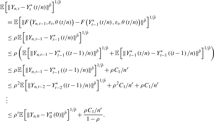
Applying the above Markov(1) argument to the stacked process
$\{\mathbf {Y} _{n,t}\}$
 gives the same bounds for
$\mathbf {Y}_{n,t}-\mathbf {Y}_t^*(t/n)$
gives the same bounds for
$\mathbf {Y}_{n,t}-\mathbf {Y}_t^*(t/n)$
 and
$\mathbf {Y}_t^*(u)-\mathbf {Y}_t^*(v)$
and
$\mathbf {Y}_t^*(u)-\mathbf {Y}_t^*(v)$
 . Since
$Y_{n,t}$
. Since
$Y_{n,t}$
 and
$Y_t^*(\cdot )$
and
$Y_t^*(\cdot )$
 are the first coordinates of
$\mathbf {Y}_{n,t}$
are the first coordinates of
$\mathbf {Y}_{n,t}$
 and
$\mathbf {Y}_t^*(\cdot )$
and
$\mathbf {Y}_t^*(\cdot )$
 , the same bounds hold for the original q-Markov process
$\{Y_{n,t}\}$
, the same bounds hold for the original q-Markov process
$\{Y_{n,t}\}$
 . Continuing the above two recursions yields the desired results.
Proof of Lemma 3
With
$\xi _{t}=\left ( \varepsilon _{t},\eta _{t}\right ) $
 and
$F\left ( y,x,\xi _{t},t/n\right ) =\left [ G\left ( y,x,\varepsilon _{t};\theta \left ( t/n\right ) \right ) ,\right.\left. H\left ( x,\eta _{t};t/n\right ) \right ] $
and
$F\left ( y,x,\xi _{t},t/n\right ) =\left [ G\left ( y,x,\varepsilon _{t};\theta \left ( t/n\right ) \right ) ,\right.\left. H\left ( x,\eta _{t};t/n\right ) \right ] $
 , the Markov process
$Z_{n,t}=\left ( Y_{n,t},X_{n,t}\right ) $
, the Markov process
$Z_{n,t}=\left ( Y_{n,t},X_{n,t}\right ) $
 satisfies
$Z_{n,t}=F\left ( Z_{n,t-1},\xi _{t},t/n\right ) $
satisfies
$Z_{n,t}=F\left ( Z_{n,t-1},\xi _{t},t/n\right ) $
 . To show existence of a stationary and
$\tau $
. To show existence of a stationary and
$\tau $
 -weakly dependent solution
$Z_{t}^{*}\left (u\right ) =\left ( Y_{t}^{*}\left ( u\right ) ,X_{t}^{*}\left ( u\right ) \right ) $
-weakly dependent solution
$Z_{t}^{*}\left (u\right ) =\left ( Y_{t}^{*}\left ( u\right ) ,X_{t}^{*}\left ( u\right ) \right ) $
 to
$Z_{t}^{*}\left ( u\right ) =F\left ( Z_{t-1}^{*}\left ( u\right ) ,\xi _{t},u\right ) $
to
$Z_{t}^{*}\left ( u\right ) =F\left ( Z_{t-1}^{*}\left ( u\right ) ,\xi _{t},u\right ) $
 , define
$\ \left \Vert z\right \Vert _{w}=\left \Vert \left ( y,x\right ) \right \Vert _{w}=\left ( \left \Vert y\right \Vert ^{p}+w\left \Vert x\right \Vert ^{p}\right ) ^{1/p}$
, define
$\ \left \Vert z\right \Vert _{w}=\left \Vert \left ( y,x\right ) \right \Vert _{w}=\left ( \left \Vert y\right \Vert ^{p}+w\left \Vert x\right \Vert ^{p}\right ) ^{1/p}$
 for some
$w>0$
for some
$w>0$
 which will be chosen below. For
$z=(y,x)$
which will be chosen below. For
$z=(y,x)$
 and
$z^{\prime }=(y^{\prime },x^{\prime })$
and
$z^{\prime }=(y^{\prime },x^{\prime })$
 , we have

Assumption 11(ii) and (iii) and Minkowski’s inequality imply that
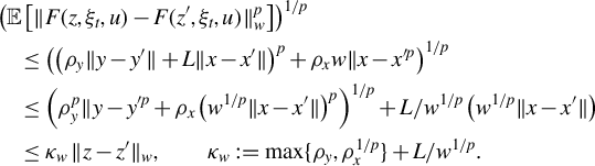
Since
$\rho _y<1$
 and
$\rho _x^{1/p}<1$
and
$\rho _x^{1/p}<1$
 , we can choose w large enough so that
$L/w^{1/p}<1-\max \{\rho _y,\rho _x^{1/p}\}$
, we can choose w large enough so that
$L/w^{1/p}<1-\max \{\rho _y,\rho _x^{1/p}\}$
 . Hence,
$F(\cdot ,\xi _t,u)$
. Hence,
$F(\cdot ,\xi _t,u)$
 is a contraction in
$L^p$
is a contraction in
$L^p$
 under
$\|\cdot \|_w$
under
$\|\cdot \|_w$
 . The existence and uniqueness of the stationary solution
$Z_t^*(u)$
. The existence and uniqueness of the stationary solution
$Z_t^*(u)$
 and geometric
$\tau $
and geometric
$\tau $
 -weak dependence then follow from Corollary 3.1 of Doukhan and Wintenberger (Reference Doukhan and Wintenberger2008), implying
$\tau _{Y,X}(k)\le C\kappa _w^k$
-weak dependence then follow from Corollary 3.1 of Doukhan and Wintenberger (Reference Doukhan and Wintenberger2008), implying
$\tau _{Y,X}(k)\le C\kappa _w^k$
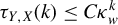 .
.
For the LS(
$\tilde {p},r$
 ) claim, combine the above contraction bound with the parameter-smoothness conditions in Assumption 11 (iv) and (v) and follow the same approximation argument as in the proof of Lemma 5.
Proof of Corollary 4
We can here apply our theory with
$\Theta =\mathbb {R}^{1+2q+d_{X}}$
 since the least-squares criterion used for estimation is concave in
$\theta $
since the least-squares criterion used for estimation is concave in
$\theta $
 (cf. the comments following Assumptions 1–3). We first show that
$Y_{n,t}$
(cf. the comments following Assumptions 1–3). We first show that
$Y_{n,t}$
 is locally stationary with
$p\geq 2$
is locally stationary with
$p\geq 2$
 moments when
$\mathbb {E}\left [ \left \Vert \varepsilon _{t}\right \Vert ^{2}\right ] <\infty $
moments when
$\mathbb {E}\left [ \left \Vert \varepsilon _{t}\right \Vert ^{2}\right ] <\infty $
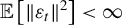 by verifying the conditions of Lemma 3 for
$ G\left ( y,x,e,\theta \right ) :=\omega +\sum _{i=1}^{q}\alpha _{1,i}y_{i}^{+}+\sum _{i=1}^{q}\alpha _{2,i}y_{i}^{-}+\gamma ^{\prime }x+e$
by verifying the conditions of Lemma 3 for
$ G\left ( y,x,e,\theta \right ) :=\omega +\sum _{i=1}^{q}\alpha _{1,i}y_{i}^{+}+\sum _{i=1}^{q}\alpha _{2,i}y_{i}^{-}+\gamma ^{\prime }x+e$
 : First,
$\mathbb {E}\left [ G\left ( 0,0,\varepsilon _{t};\theta \right ) ^{2} \right ] =\mathbb {E}\left [ \varepsilon _{t}^{2}\right ] <\infty $
: First,
$\mathbb {E}\left [ G\left ( 0,0,\varepsilon _{t};\theta \right ) ^{2} \right ] =\mathbb {E}\left [ \varepsilon _{t}^{2}\right ] <\infty $
 ; second, for all
$y,y\in \mathcal {\mathbb {R}}^{q}$
; second, for all
$y,y\in \mathcal {\mathbb {R}}^{q}$
 and
$x,x^{\prime }\in \mathcal {\mathbb { R}}^{d_{X}}$
and
$x,x^{\prime }\in \mathcal {\mathbb { R}}^{d_{X}}$
 ,
,

third, for all
$\theta ,\theta ^{\prime }\in \Theta $
 ,
,

Thus, under (22),
$\left ( Y_{n,t},X_{n,t}\right ) $
 is locally stationary with
$\left ( Y_{t}^{\ast }\left ( u\right ) ,X_{t}^{\ast }\left ( u\right ) \right ) $
is locally stationary with
$\left ( Y_{t}^{\ast }\left ( u\right ) ,X_{t}^{\ast }\left ( u\right ) \right ) $
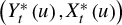 being
$\tau $
being
$\tau $
 -weakly dependent,
$\mathbb {E}\left [ Y_{t}^{\ast }\left ( u\right ) ^{2}\right ] <\infty $
-weakly dependent,
$\mathbb {E}\left [ Y_{t}^{\ast }\left ( u\right ) ^{2}\right ] <\infty $
 and
$\mathbb {E}\left [ \left \Vert X_{t}^{\ast }\left ( u\right ) \right \Vert ^{2}\right ] <\infty $
and
$\mathbb {E}\left [ \left \Vert X_{t}^{\ast }\left ( u\right ) \right \Vert ^{2}\right ] <\infty $
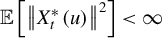 . Next, write
$\ell _{n,t}\left ( \theta \right ) =-\left ( Y_{n,t}-\theta ^{\prime }\tilde {X}_{n,t}\right ) ^{2}$
. Next, write
$\ell _{n,t}\left ( \theta \right ) =-\left ( Y_{n,t}-\theta ^{\prime }\tilde {X}_{n,t}\right ) ^{2}$
 , where
$\tilde {X}_{n,t}=\left ( 1,Y_{n,t-1}^{+},\dots ,Y_{n,t-q}^{+},Y_{n,t-1}^{-},\dots ,Y_{n,t-q}^{-},X_{n,t-1}^{\prime }\right ) ^{\prime } $
, where
$\tilde {X}_{n,t}=\left ( 1,Y_{n,t-1}^{+},\dots ,Y_{n,t-q}^{+},Y_{n,t-1}^{-},\dots ,Y_{n,t-q}^{-},X_{n,t-1}^{\prime }\right ) ^{\prime } $
 , so that
$s_{n,t}=\varepsilon _{t}\tilde {X}_{n,t}$
, so that
$s_{n,t}=\varepsilon _{t}\tilde {X}_{n,t}$
 and
$h_{n,t}\left ( \theta \right ) =\tilde {X}_{n,t}\tilde {X}_{n,t}^{\prime }$
and
$h_{n,t}\left ( \theta \right ) =\tilde {X}_{n,t}\tilde {X}_{n,t}^{\prime }$
 . It is easily seen that
$\ell _{n,t}\left ( \theta \right ) $
. It is easily seen that
$\ell _{n,t}\left ( \theta \right ) $
 ,
$s_{n,t}s_{n,t}^{\prime }$
,
$s_{n,t}s_{n,t}^{\prime }$
 , and
$ h_{n,t}\left ( \theta \right ) $
, and
$ h_{n,t}\left ( \theta \right ) $
 satisfy the second part of Lemma 1 with
$s=1$
satisfy the second part of Lemma 1 with
$s=1$
 and
$p_{1}=2$
and
$p_{1}=2$
 so that they are all ULS
$\left ( 1,1,\Theta \right ) $
so that they are all ULS
$\left ( 1,1,\Theta \right ) $
 . It now follows from the first part of Corollary 3 that Theorem 2 applies to the local linear estimator.
Next, we verify the conditions of the second part of Corollary 3. First, note that Lemma 3 implies that if
$ \mathbb {E}\left [ \varepsilon _{t}^{4}\right ] <\infty , $
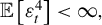 then
$\mathbb {E[} Y_{t}^{\ast }\left ( u\right ) ^{4}]<\infty $
then
$\mathbb {E[} Y_{t}^{\ast }\left ( u\right ) ^{4}]<\infty $
 and so
$h_{t}^{\ast }\left ( \theta \left ( u\right ) |u\right ) =\tilde {X}_{t}^{\ast }\left ( u\right ) \tilde {X}_{t}^{\ast }\left ( u\right ) ^{\prime }$
and so
$h_{t}^{\ast }\left ( \theta \left ( u\right ) |u\right ) =\tilde {X}_{t}^{\ast }\left ( u\right ) \tilde {X}_{t}^{\ast }\left ( u\right ) ^{\prime }$
 is
$\tau $
is
$\tau $
 -weakly dependent with
$\mathbb {E}\left [ \left \Vert h_{t}^{\ast }\left ( \theta \left ( u\right ) |u\right ) \right \Vert ^{2}\right ] <\infty $
-weakly dependent with
$\mathbb {E}\left [ \left \Vert h_{t}^{\ast }\left ( \theta \left ( u\right ) |u\right ) \right \Vert ^{2}\right ] <\infty $
 , and hence Assumption 10 is satisfied. Finally, to verify Assumption 7, we show that
$\partial _{u}h_{t}^{\ast }\left ( \theta \left ( u\right ) |u\right ) =2\tilde {X}_{t}^{\ast }\left ( u\right ) \partial _{u}\tilde {X}_{t}^{\ast }\left ( u\right ) ^{\prime }$
, and hence Assumption 10 is satisfied. Finally, to verify Assumption 7, we show that
$\partial _{u}h_{t}^{\ast }\left ( \theta \left ( u\right ) |u\right ) =2\tilde {X}_{t}^{\ast }\left ( u\right ) \partial _{u}\tilde {X}_{t}^{\ast }\left ( u\right ) ^{\prime }$
 is well-defined almost surely and has first moments. This will hold if
$ \partial _{u}\left ( Y_{t}^{\ast }\left ( u\right ) ,X_{t}^{\ast }\left ( u\right ) \right ) $
is well-defined almost surely and has first moments. This will hold if
$ \partial _{u}\left ( Y_{t}^{\ast }\left ( u\right ) ,X_{t}^{\ast }\left ( u\right ) \right ) $
 exists almost surely and has second moments. We show this by applying Theorem 4.8 of Dahlhaus et al. (Reference Dahlhaus, Richter and Wu2019). This theorem requires
$ G\left ( y,x,\varepsilon _{t};\theta \right ) $
exists almost surely and has second moments. We show this by applying Theorem 4.8 of Dahlhaus et al. (Reference Dahlhaus, Richter and Wu2019). This theorem requires
$ G\left ( y,x,\varepsilon _{t};\theta \right ) $
 to be differentiable w.r.t.
$ \left ( y,x,\theta \right ) $
to be differentiable w.r.t.
$ \left ( y,x,\theta \right ) $
 for all values of
$\left ( y,x,\theta \right ) $
for all values of
$\left ( y,x,\theta \right ) $
 which fails to hold at
$y=0$
which fails to hold at
$y=0$
 . However, since
$\varepsilon _{t}$
. However, since
$\varepsilon _{t}$
 is assumed to have a continuous distribution then
$Y_{t}^{\ast }\left ( u\right ) | \mathcal {F}_{t-1}^{\ast }\left ( u\right ) $
is assumed to have a continuous distribution then
$Y_{t}^{\ast }\left ( u\right ) | \mathcal {F}_{t-1}^{\ast }\left ( u\right ) $
 will also have a continuous distribution and so
$\Pr \left ( Y_{t}^{\ast }\left ( u\right ) =0|\mathcal {F} _{t-1}^{\ast }\left ( u\right ) \right ) =0$
will also have a continuous distribution and so
$\Pr \left ( Y_{t}^{\ast }\left ( u\right ) =0|\mathcal {F} _{t-1}^{\ast }\left ( u\right ) \right ) =0$
 . Thus,
$G\left ( Y_{t-1}^{\ast }\left ( u\right ) ,\dots ,Y_{t-q}^{\ast }\left ( u\right ) ,X_{t-1}^{\ast }\left ( u\right ) .\varepsilon _{t};\theta \right ) $
. Thus,
$G\left ( Y_{t-1}^{\ast }\left ( u\right ) ,\dots ,Y_{t-q}^{\ast }\left ( u\right ) ,X_{t-1}^{\ast }\left ( u\right ) .\varepsilon _{t};\theta \right ) $
 is differentiable w.r.t.
$\left ( Y_{t-1}^{\ast }\left ( u\right ) ,\dots ,Y_{t-q}^{\ast }\left ( u\right ) ,X_{t-1}^{\ast }\left ( u\right ) ,\theta \right ) $
is differentiable w.r.t.
$\left ( Y_{t-1}^{\ast }\left ( u\right ) ,\dots ,Y_{t-q}^{\ast }\left ( u\right ) ,X_{t-1}^{\ast }\left ( u\right ) ,\theta \right ) $
 almost surely. By inspection of the proof of Theorem 4.8, this suffices for the result to hold.
Proof of Corollary 5
We verify the conditions of Corollary 3. Verification of the conditions for the stationary version, including identification and existence of relevant moments, follows from Kristensen and Rahbek (Reference Kristensen and Rahbek2005). For the analysis of the local linear estimator, what remains to be shown is uniform local stationarity of
$\ell _{n,t}\left ( \theta \right ) $
 ,
$ s_{n,t}s_{n,t}^{\prime }$
,
$ s_{n,t}s_{n,t}^{\prime }$
 , and
$h_{n,t}\left ( \theta \right ) $
, and
$h_{n,t}\left ( \theta \right ) $
 . First, by Lemma 3 with
$G\left ( y,x,\varepsilon ,\theta \right ) =\left ( \omega +\sum _{i=1}^{q}\alpha _{i}y_{i}+\gamma ^{\prime }x\right ) \varepsilon ^{2}$
. First, by Lemma 3 with
$G\left ( y,x,\varepsilon ,\theta \right ) =\left ( \omega +\sum _{i=1}^{q}\alpha _{i}y_{i}+\gamma ^{\prime }x\right ) \varepsilon ^{2}$
 , where
$\sum _{i=1}^{q}\alpha _{i}<1$
, where
$\sum _{i=1}^{q}\alpha _{i}<1$
 , it follows that
$ \left ( Y_{n,t},X_{n,t}\right ) $
, it follows that
$ \left ( Y_{n,t},X_{n,t}\right ) $
 is locally stationary with
$\sup _{n,t} \mathbb {E}\left [ Y_{n,t}^{2}\right ] <\infty $
is locally stationary with
$\sup _{n,t} \mathbb {E}\left [ Y_{n,t}^{2}\right ] <\infty $
 and
$\mathbb {E}\left [ Y_{t}^{\ast }\left ( u\right ) ^{2}\right ] <\infty $
and
$\mathbb {E}\left [ Y_{t}^{\ast }\left ( u\right ) ^{2}\right ] <\infty $
 . Next, we verify that
$ \ell _{n,t}\left ( \theta \right ) $
. Next, we verify that
$ \ell _{n,t}\left ( \theta \right ) $
 and its first two derivatives satisfy the conditions of Lemma 1.
Recall that
$\ell _{n,t}\left ( \theta \right ) =\log \left ( \lambda _{n,t}\left ( \theta \right ) \right ) +Y_{n,t}/\lambda _{n,t}\left ( \theta \right ) $
 with
$\tilde {X}_{n,t}=\left ( 1,Y_{n,t-1},\ldots ,\right.\left. Y_{n,t-q},X_{n,t-1}^{\prime }\right ) ^{\prime }$
with
$\tilde {X}_{n,t}=\left ( 1,Y_{n,t-1},\ldots ,\right.\left. Y_{n,t-q},X_{n,t-1}^{\prime }\right ) ^{\prime }$
 and
$ \lambda _{n,t}\left ( \theta \right ) =\theta ^{\prime }\tilde {X}_{n,t}$
and
$ \lambda _{n,t}\left ( \theta \right ) =\theta ^{\prime }\tilde {X}_{n,t}$
 . It satisfies

where

Since
$\varepsilon _{t}^{2}=Y_{n,t}/\lambda _{n,t}\left ( \theta \right ) $
 ,
$ \ell _{n,t}\left ( \theta \right ) $
,
$ \ell _{n,t}\left ( \theta \right ) $
 satisfies the second part of Lemma 1 with
$g\left ( Z_{n,t}\right ) =C\left ( 1+Y_{n,t}/\lambda _{n,t}\left ( \theta (t/n)\right ) \right ) =C\left ( 1+\varepsilon _{t}^{2}\right ) $
satisfies the second part of Lemma 1 with
$g\left ( Z_{n,t}\right ) =C\left ( 1+Y_{n,t}/\lambda _{n,t}\left ( \theta (t/n)\right ) \right ) =C\left ( 1+\varepsilon _{t}^{2}\right ) $
 , which has second moment by assumption. Thus, Lemma 1 implies that
$\ell _{n,t}\left ( \theta \right ) $
, which has second moment by assumption. Thus, Lemma 1 implies that
$\ell _{n,t}\left ( \theta \right ) $
 is ULS
$\left ( 1,1,\Theta \right ) $
is ULS
$\left ( 1,1,\Theta \right ) $
 .
.
Next, we analyze the score function

Since
$\mathbb {E}\left [ \varepsilon _{t}^{2}|\mathcal {F}_{n,t-1}\right ] = \mathbb {E}\left [ \varepsilon _{t}^{2}\right ] =1$
 ,
$s_{n,t}\left ( \theta \left ( t/n\right ) \right ) $
,
$s_{n,t}\left ( \theta \left ( t/n\right ) \right ) $
 is an MGD. Moreover,
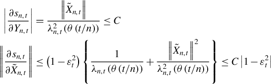
and so
$s_{n,t}$
 satisfies the conditions of Lemma 1 with
$g\left ( Z_{n,t}\right ) =C\left ( 1+\varepsilon _{t}^{2}\right ) $
satisfies the conditions of Lemma 1 with
$g\left ( Z_{n,t}\right ) =C\left ( 1+\varepsilon _{t}^{2}\right ) $
 .
.
The Hessian takes the form

and recycling the inequalities established above it follows that the Hessian is also ULS(1,1,
$\Theta $
 ). This verifies the conditions for Theorem 2.
For the analysis of the local constant estimator, observe that
$ h_{ij,t}^{\ast }\left ( \theta \left ( u\right ) |u\right ) $
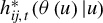 is
$\tau $
is
$\tau $
 -weakly dependent by Lemma 1; moreover, if
$\mathbb {E}\left [ \lVert \varepsilon _{t}\rVert ^{4+\gamma }\right ] <\infty , $
-weakly dependent by Lemma 1; moreover, if
$\mathbb {E}\left [ \lVert \varepsilon _{t}\rVert ^{4+\gamma }\right ] <\infty , $
 then
$\mathbb {E} \left [ \lVert h_{ij,t}^{\ast }\left ( \theta \left ( u\right ) |u\right ) \rVert |^{2+\gamma /2}\right ] <\infty $
then
$\mathbb {E} \left [ \lVert h_{ij,t}^{\ast }\left ( \theta \left ( u\right ) |u\right ) \rVert |^{2+\gamma /2}\right ] <\infty $
 . Thus, Assumption 10 holds. To verify Assumption 9, first note that
$\partial _{u}X_{t}^{\ast }\left ( u\right ) $
. Thus, Assumption 10 holds. To verify Assumption 9, first note that
$\partial _{u}X_{t}^{\ast }\left ( u\right ) $
 exists under the assumptions of the theorem. We then follow the same arguments as in Example 5.5 of Dahlhaus et al. (Reference Dahlhaus, Richter and Wu2019) to show that
$ \partial _{u}h_{ij,t}^{\ast }\left ( \theta |u\right ) $
exists under the assumptions of the theorem. We then follow the same arguments as in Example 5.5 of Dahlhaus et al. (Reference Dahlhaus, Richter and Wu2019) to show that
$ \partial _{u}h_{ij,t}^{\ast }\left ( \theta |u\right ) $
 exists.
Proof of Corollary 6
We first show that the
$\left ( Y_{n,t},X_{n,t}\right ) $
 is locally stationary by verifying the conditions of Lemma 3 with
$ G\left ( y,x,\varepsilon _{t};\theta \right ) :=N_{t}\left ( \omega +\sum _{i=1}^{q}\alpha _{i}y_{i}+\gamma ^{\prime }x\right ) $
is locally stationary by verifying the conditions of Lemma 3 with
$ G\left ( y,x,\varepsilon _{t};\theta \right ) :=N_{t}\left ( \omega +\sum _{i=1}^{q}\alpha _{i}y_{i}+\gamma ^{\prime }x\right ) $
 , where
$ \varepsilon _{t}:=N_{t}\left ( \cdot \right ) $
, where
$ \varepsilon _{t}:=N_{t}\left ( \cdot \right ) $
 ,
$t=1,2,\ldots $
,
$t=1,2,\ldots $
 , are i.i.d. copies of a Poisson process (see Agosto et al., Reference Agosto, Cavaliere, Kristensen and Rahbek2016 for details): First,
$ \mathbb {E}\left [ \left \vert G\left ( 0,0,\varepsilon _{t};\theta \left ( u\right ) \right ) \right \vert \right ] \leq \mathbb {E}\left [ N_{t}\left ( \omega \left ( u\right ) \right ) \right ] =\omega \left (u\right ) <\infty $
, are i.i.d. copies of a Poisson process (see Agosto et al., Reference Agosto, Cavaliere, Kristensen and Rahbek2016 for details): First,
$ \mathbb {E}\left [ \left \vert G\left ( 0,0,\varepsilon _{t};\theta \left ( u\right ) \right ) \right \vert \right ] \leq \mathbb {E}\left [ N_{t}\left ( \omega \left ( u\right ) \right ) \right ] =\omega \left (u\right ) <\infty $
 ; second, for all
$x,y,x^{\prime },y^{\prime }$
; second, for all
$x,y,x^{\prime },y^{\prime }$
 ,
,
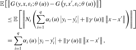
where
$\sum _{i=1}^{q}\alpha _{i}\left ( u\right ) <1$
 . Finally, for any
$ \theta ,\theta ^{\prime }$
. Finally, for any
$ \theta ,\theta ^{\prime }$
 ,
,

Thus,
$\lambda _{n,t}\left ( \theta \right ) $
 and
$Y_{n,t}$
and
$Y_{n,t}$
 are ULS
$\left ( 1,1,\Theta \right ) $
are ULS
$\left ( 1,1,\Theta \right ) $
 . From Agosto et al. (Reference Agosto, Cavaliere, Kristensen and Rahbek2016), we also know that
$\mathbb {E} \left [ \lambda _{t}^{\ast }\left (u\right ) ^{2}\right ] <\infty $
. From Agosto et al. (Reference Agosto, Cavaliere, Kristensen and Rahbek2016), we also know that
$\mathbb {E} \left [ \lambda _{t}^{\ast }\left (u\right ) ^{2}\right ] <\infty $
 , and hence
$ \mathbb {E}[Y_{t}^{\ast }\left ( u\right )^{2} ]<\infty $
, and hence
$ \mathbb {E}[Y_{t}^{\ast }\left ( u\right )^{2} ]<\infty $
 too.
too.
Next, we observe that
$\lambda _{n,t}\left ( \theta \right ) $
 ,
$\partial _{\theta }\lambda _{n,t}\left ( \theta \right ) $
,
$\partial _{\theta }\lambda _{n,t}\left ( \theta \right ) $
 , and
$\partial _{\theta \theta }^{2}\lambda _{n,t}\left ( \theta \right ) $
, and
$\partial _{\theta \theta }^{2}\lambda _{n,t}\left ( \theta \right ) $
 are on the same form as in the GARCH model. In particular, it is easily checked that
$\lambda _{n,t}\left ( \theta \right ) ,\, \partial _{\theta }\lambda _{n,t}\left ( \theta \right ) $
are on the same form as in the GARCH model. In particular, it is easily checked that
$\lambda _{n,t}\left ( \theta \right ) ,\, \partial _{\theta }\lambda _{n,t}\left ( \theta \right ) $
 , and
$\partial _{\theta \theta }^{2}\lambda _{n,t}\left ( \theta \right ) $
, and
$\partial _{\theta \theta }^{2}\lambda _{n,t}\left ( \theta \right ) $
 are ULS
$\left ( 1,1,\Theta \right ) $
are ULS
$\left ( 1,1,\Theta \right ) $
 and with their stationary versions having second moments. This in turn implies that the log-likelihood and its first two derivatives w.r.t.
$\theta $
and with their stationary versions having second moments. This in turn implies that the log-likelihood and its first two derivatives w.r.t.
$\theta $
 satisfy the conditions of Lemma 1. First,

where
$\lambda _{n,t}\left ( \theta \right ) $
 has second moment. Second,

where again the right-hand side has second moment. The score function takes the form
$s_{n,t}=\left ( Y_{n,t}/\lambda _{n,t}\left ( \theta \left ( t/n\right ) \right ) -1\right ) \partial _{\theta }\lambda _{n,t}\left ( \theta \left ( t/n\right ) \right ) $
 which satisfies the MGD condition. It is easily checked that
$s_{n,t}$
which satisfies the MGD condition. It is easily checked that
$s_{n,t}$
 is LS
$\left ( 2,1\right ) $
is LS
$\left ( 2,1\right ) $
 . Similarly,

is ULS
$\left ( 1,1,\Theta \right ) $

Finally, for the local constant estimator, we need to show that
$\partial _{u}H\left ( u\right ) $
 exists. We do this for the case of
$q=1$
exists. We do this for the case of
$q=1$
 to keep notation simple; the general case follows by the same arguments. We show existence by verifying the conditions SC1–SC3 of Truquet (Reference Truquet2020) under which the result will follow (cf. Proposition 2 of the same paper). First observe that the transition kernel of the Markov chain
$\left ( Y_{t}^{\ast },X_{t}^{\ast }\right ) \left ( u\right ) |\left ( Y_{t-1}^{\ast },X_{t-1}^{\ast }\right ) \left ( u\right ) $
to keep notation simple; the general case follows by the same arguments. We show existence by verifying the conditions SC1–SC3 of Truquet (Reference Truquet2020) under which the result will follow (cf. Proposition 2 of the same paper). First observe that the transition kernel of the Markov chain
$\left ( Y_{t}^{\ast },X_{t}^{\ast }\right ) \left ( u\right ) |\left ( Y_{t-1}^{\ast },X_{t-1}^{\ast }\right ) \left ( u\right ) $
 takes the form

where
$\lambda \left ( y_{0},x_{0};u\right ) =\omega \left ( u\right ) +\alpha \left ( u\right ) y_{0}+\gamma \left ( u\right ) ^{\prime }x_{0}$
 . It satisfies
$ q\left ( y,x|y_{0},x_{0};u\right )>0$
. It satisfies
$ q\left ( y,x|y_{0},x_{0};u\right )>0$
 for all
$\left ( y,x,y_{0},x_{0},u\right ) $
for all
$\left ( y,x,y_{0},x_{0},u\right ) $
 under the assumptions of the corollary. Moreover, by the same arguments as in the proof of Proposition 4 of Truquet (Reference Truquet2020),

for some
$b<\infty $
 with
$d_{0}=2$
with
$d_{0}=2$
 . This combined with the drift criterion imposed on
$X_{t}^{\ast }\left ( u\right ) $
. This combined with the drift criterion imposed on
$X_{t}^{\ast }\left ( u\right ) $
 implies that SC1 is satisfied with
$\phi \left ( y,x\right ) =1+\left \vert y\right \vert +\left \Vert x\right \Vert $
implies that SC1 is satisfied with
$\phi \left ( y,x\right ) =1+\left \vert y\right \vert +\left \Vert x\right \Vert $
 and
$d_{0}=1$
and
$d_{0}=1$
 . The transition kernel is differentiable under the assumptions of the corollary and so SC2 is satisfied with
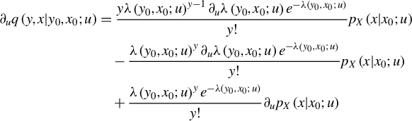
so that, applying the restrictions on
$p_{X}\left ( x|x_{0};u\right ) $
 ,
,

Thus, by the same arguments as in the proof of Proposition 4 of Truquet (Reference Truquet2020),
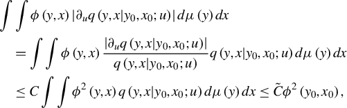
where
$\mu \left ( y\right ) $
 denotes the counting measure. Finally,
$q\left ( y,x|y_{0},x_{0};u\right ) \leq \bar {q}\left ( y,x|y_{0},x_{0}\right ) $
denotes the counting measure. Finally,
$q\left ( y,x|y_{0},x_{0};u\right ) \leq \bar {q}\left ( y,x|y_{0},x_{0}\right ) $
 where, with
$\bar {p}_{X}^{\left ( 0\right ) }\left ( x|x_{0}\right ) $
where, with
$\bar {p}_{X}^{\left ( 0\right ) }\left ( x|x_{0}\right ) $
 defined in the corollary,

here,
$\bar {\lambda }\left ( y_{0},x_{0}\right ) =\bar {\omega }+\bar {\alpha } y_{0}+\bar {\gamma }^{\prime }x_{0}$
 ,
$\underline {\lambda }\left ( y_{0},x_{0};u\right ) =\underline {\omega }+\underline {\alpha }y_{0}+ \underline {\gamma }^{\prime }x_{0}$
,
$\underline {\lambda }\left ( y_{0},x_{0};u\right ) =\underline {\omega }+\underline {\alpha }y_{0}+ \underline {\gamma }^{\prime }x_{0}$
 with
$\bar {\omega }=\max _{v\in \left [ u-\epsilon ,u+\epsilon \right ] }\omega \left ( u\right ) $
with
$\bar {\omega }=\max _{v\in \left [ u-\epsilon ,u+\epsilon \right ] }\omega \left ( u\right ) $
 ,
$\underline {\omega }=\min _{v\in \left [ u-\epsilon ,u+\epsilon \right ] }\omega \left ( u\right ) $
,
$\underline {\omega }=\min _{v\in \left [ u-\epsilon ,u+\epsilon \right ] }\omega \left ( u\right ) $
 and similarly for the other constants. Since
$\int \int \phi ^{2}\left ( y,x\right ) \bar {q}\left ( y,x|y_{0},x_{0}\right ) d\mu \left ( y\right ) dx<\infty $
and similarly for the other constants. Since
$\int \int \phi ^{2}\left ( y,x\right ) \bar {q}\left ( y,x|y_{0},x_{0}\right ) d\mu \left ( y\right ) dx<\infty $
 , it follows by dominated convergence that

A similar bound can be obtained for
$\left \vert \partial _{u}q\left ( y,x|y_{0},x_{0};u\right ) \right \vert $
 so that

This completes the proof.
FUNDING STATEMENT
The authors declare that no specific funding has been received for this article.
COMPETING INTEREST
The authors declare that no competing interests exist.


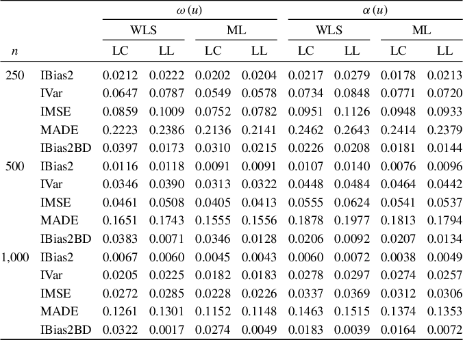
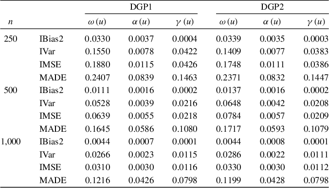
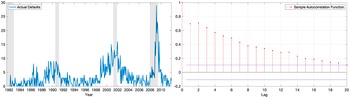
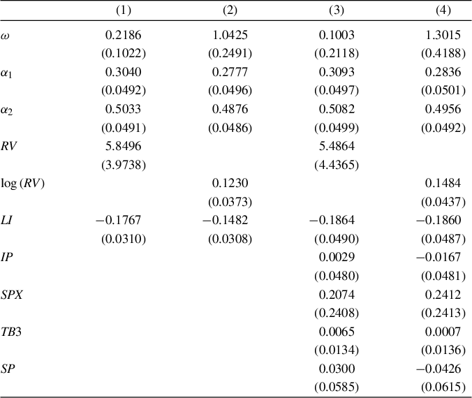
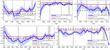
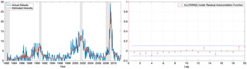
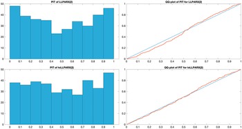
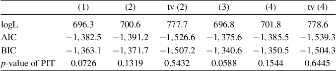
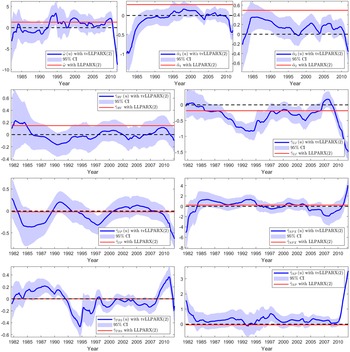

 Open access

