


1. Introduction
As Arctic sea ice has declined in extent and volume in recent decades (Serreze and Meier, Reference Serreze and Meier2019; Walsh and others, Reference Walsh, Eicken, Redilla and Johnson2022), several human activities, such as shipping and tourism, have become more common in the Arctic (Pizzolato and others, Reference Pizzolato, Howell, Dawson, Laliberté and Copland2016; Wagner, Reference Wagner2020; Gunnarsson, Reference Gunnarsson2021). This has inspired investigation into seasonal forecasting of Arctic sea-ice conditions (Boisvert and others, Reference Boisvert, Petty and Stroeve2016; Horvath and others, Reference Horvath, Stroeve, Rajagopalan and Kleiber2020; Blanchard‐Wrigglesworth, Reference Blanchard‐Wrigglesworth2023), as well as sub-seasonal (daily to weekly) forecasting (Liu and others, Reference Liu, Wang and Kumar2018; Wayand and others, Reference Wayand, Bitz and Blanchard‐Wrigglesworth2019; McGraw and others, Reference McGraw, Blanchard-Wrigglesworth, Clancy and Bitz2022). Of particular interest on the sub-seasonal scale are rapid ice loss events (RILEs) over 5–7 days, which can occur regionally throughout the year but are strictly summer phenomena if looking Arctic-wide (Stroeve and Notz, Reference Stroeve and Notz2018; Wang and others, Reference Wang, Walsh, Szymborski and Peng2020; McGraw and others, Reference McGraw, Blanchard-Wrigglesworth, Clancy and Bitz2022). Dynamical forecasting models have shown less skill in predicting sea-ice extent (SIE) during such events (McGraw and others, Reference McGraw, Blanchard-Wrigglesworth, Clancy and Bitz2022). Although RILEs have received the most attention, other large anomalies in SIE tendency include rapid sea-ice growth events (Stroeve and Notz, Reference Stroeve and Notz2018) or, looking seasonally, pauses in SIE expansion during autumn/winter and pauses in SIE contraction during summer. Better understanding of the frequency, drivers and trends in such extreme events in SIE tendency will be an asset to sub-seasonal sea-ice prediction.
In this study, we focus on pauses in SIE expansion during autumn (i.e. when the 6 day change in SIE < 0 km2). Similar to RILEs, pauses in SIE expansion represent a negative anomaly for SIE tendency, so the drivers of each event type are likely similar. Several regional RILEs have been linked to severe extratropical cyclones (Zhang and others, Reference Zhang, Lindsay, Schweiger and Steele2013; Boisvert and others, Reference Boisvert, Petty and Stroeve2016). However, because extratropical cyclone impacts on sea ice are dependent on storm intensity (Kriegsmann and Brümmer, Reference Kriegsmann and Brümmer2014; Aue and others, Reference Aue, Vihma, Uotila and Rinke2022), location relative to the sea-ice edge and coastline (Lukovich, Reference Lukovich2021; Clancy and others, Reference Clancy, Bitz, Blanchard-Wrigglesworth, McGraw and Cavallo2022; Aue and Rinke, Reference Aue and Rinke2023), the season of occurrence (Schreiber and Serreze, Reference Schreiber and Serreze2020; Finocchio and Doyle, Reference Finocchio and Doyle2021; Clancy and others, Reference Clancy, Bitz, Blanchard-Wrigglesworth, McGraw and Cavallo2022) and the interplay of direct and indirect impacts from radiation, wind forcing and snowfall (Graham, Reference Graham2019; Schreiber and Serreze, Reference Schreiber and Serreze2020; Peng, Reference Peng2021; Dethloff, Reference Dethloff2022), the presence of a strong extratropical cyclone alone is insufficient to predict how the sea-ice cover will respond.
In their assessment of atmospheric drivers of regional summer RILEs, Wang and others (Reference Wang, Walsh, Szymborski and Peng2020) found that southerly wind anomalies and enhanced water vapor transport over the region experiencing the RILE were associated with a dipole pattern in the 500 hPa geopotential height with an anomalous high and low to the east and west, respectively. These events were also frequently linked to anticyclonic Rossby wave breaking (Wang and others, Reference Wang, Walsh, Szymborski and Peng2020). However, they also found that enhanced poleward transport of heat and moisture in one Arctic region was typically mirrored by equatorward anomalies elsewhere, making it likely that counteracting anomalies in atmospheric variables or SIE tendency may cancel each other out if considering an Arctic-wide scale. Therefore, an Arctic-wide pause in autumn SIE expansion may require more specific conditions.
The long-term decline in Arctic sea-ice thickness and extent has several implications for how SIE tendency extremes like RILEs or pauses in autumn SIE expansion respond to atmospheric anomalies. Several studies note the importance of sea-ice properties, especially thickness, to how sea ice responds to atmospheric variability, with thinner ice being more susceptible to atmospheric forcing (Holland and others, Reference Holland, Bitz and Tremblay2006; Ricker, Reference Ricker2017; Aue and others, Reference Aue, Vihma, Uotila and Rinke2022). This suggests that the long-term thinning of sea ice ought to make for greater synoptic-scale variability in the rate of Arctic sea-ice growth in autumn. Rapid sea-ice growth events, sometimes exceeding 1 million km2 over 7 days, have become more frequent starting in 2005, especially later in the year (Stroeve and Notz, Reference Stroeve and Notz2018). Perhaps the opposite extreme anomaly, a pause in sea-ice growth, has also become more frequent. Or perhaps the increase in rapid ice-growth events simply reflects a negative feedback toward stronger autumn SIE growth in response to summer SIE loss.
This paper presents a close examination of pauses in autumn SIE expansion. After describing data and methods (Section 2), we catalog sub-seasonal pauses in autumn SIE expansion (Section 3.1), describe their regional characteristics (Section 3.2), investigate their atmospheric drivers with several case studies (Section 3.3) and evaluate the impact of long-term Arctic climate change on their occurrence (Section 3.4). Discussion and conclusions follow in Section 4.
2. Data and methods
2.1. Sea-ice extent
Arctic-wide SIE is defined as the sum of the area of ocean grid cells for which sea-ice concentration (SIC) > 15% in one of three SIC products from the National Snow and Ice Data Center (NSIDC). These products are
1) Version 4 of the NOAA/NSIDC Climate Data Record (NSIDC ID: G02202; Meier and others, Reference Meier, Fetterer, Windnagel and Stewart2021), hereafter ‘CDR’
2) Version 4 of Bootstrap SIC (NSIDC ID: 0079; Comiso, Reference Comiso2023)
3) Version 2 of NASA Team SIC (NSIDC ID: 0051; DiGirolamo and others, Reference DiGirolamo, Parkinson, Cavalieri, Gloersen and Zwally2022)
All utilize the combined passive microwave record (1979–2022) from the Scanning Multichannel Microwave Radiometer (SMMR) instrument on the Nimbus-7 satellite and the Special Sensor Microwave/Imager (SSM/I) and Special Sensor Microwave Imager/Sounder (SSMIS) instruments aboard the F-series satellites. This record has a 25 km spatial resolution on a north polar stereographic grid and Arctic-wide coverage every 2 days before 20 August 1987 and daily thereafter; however, a sizeable data gap between 3 December 1987 and 13 January 1988 limits analysis for that year. Some spatial data gaps also exist in these records, with the pole hole being spatially interpolated.
The Bootstrap and NASA Team products are derived from algorithms that utilize different combinations of microwave frequencies and polarizations. Among other differences, the Bootstrap algorithm uses daily tie-points, whereas the NASA Team algorithm uses fixed tie points and incorporates higher-frequency channels (e.g. 85–89 GHz) (Comiso and others, Reference Comiso, Cavalieri, Parkinson and Gloersen1997). Because of under-estimation of SIC under certain conditions (e.g. ice without snow cover in autumn, melt-ponding in summer), the CDR takes the maximum SIC as determined by the NASA Team and Bootstrap algorithms (Meier and others, Reference Meier, Peng, Scott and Savoie2014). One of the benefits of the CDR that makes it more appropriate for climate change analysis is that its quality control steps are all automated and homogeneous through time. However, this means that the applications of the NASA Team and Bootstrap algorithms used for the CDR (NSIDC ID: G02202) do not produce results identical to Version 4 of the Bootstrap SIC product (NSIDC ID: 0079) or Version 2 of the NASA Team SIC product (NSIDC ID: 0051), both of which involve manual quality control. All three products are used to define SIE expansion pauses, but the CDR is used to show SIC or SIE in figures unless specified.
Changes in SIE are examined using a discrete 6 day difference in Arctic-wide SIE (∆SIE). For example, if SIE on 1 December is 10.5 million km2 and SIE on 6 December is 10.4 million km2, then ∆SIE = −0.1 million km2. Using a 6 day timescale reduces sensitivity to retrieval errors and spatial interpolation of missing pixels. For this paper, a ‘pause’ in autumn (October–December) Arctic-wide SIE expansion is identified when three criteria are met:
1. ∆SIE < 0 km2 for at least one of the three SIE records (CDR, NASA Team or Bootstrap).
2. ∆SIE < 0.1 million km2 for all three SIE records.
3. At least 3 of the 6 days in the 6 day pause are in October–December.
Identification of pause events exhibits some sensitivity to the product used (Supplementary Fig. S1), and combining products ensures we examine only pause events robust to that sensitivity. Hereafter, all pauses are referred to using the date at the start of the 6 day period. If multiple 6 day pauses overlap each other, they are consolidated into a single event, and the start date of the minimum 6 day ∆SIE in the CDR is used as the reference date.
2.2. Sea-ice thickness, motion and age
Several altimetry-based gridded ice thickness products are considered, including
1. October–November ice thickness from the Glacier Laser Altimeter System aboard the ICESat satellite (NSIDC ID: ISSITGR4; Petty and Kurtz, Reference Petty and Kurtz2023) available for 2003–07.
2. October–December ice thickness from ICESat2 (NSIDC ID: IS2SITMOGR4 version 3; Petty et al.., Reference Petty and Kurtz2023) for 2018–22.
3. October–December ice thickness from CyroSat-2 synthetic aperture radar from NSIDC (ID: RDEFT4; Kurtz and Harbeck, Reference Kurtz and Harbeck2017) for 2010–22 (hereafter CS2-NSIDC).
4. October–December ice thickness from a combination of CyroSat-2 and the Soil Moisture and Ocean Salinity (CS2MOS), provided by the Alfred Wegener Institute (European Space Agency (ESA), 2023) for 2010–22.
However, a longer homogeneous record is necessary to identify regime shifts, so we also use monthly sea-ice thickness retrieved from brightness temperatures acquired by the SSM/I and SSMIS passive microwave radiometers over October–December for 1992–2023. This dataset is a statistical inversion from the ICESat-2 sea-ice thickness product (Soriot and others, Reference Soriot, Prigent, Jimenez and Frappart2023) and has shown good agreement (r = 0.88, rmsd = 0.58 m) with the CS2SMOS sea-ice thickness product over the 2018–19 winter, and strong correlation over the time series (1992–2024) with sea-ice thickness from the Pan-Arctic Ice Ocean Modeling and Assimilation System (PIOMAS; r = 0.79, bias = 0.53 m).
Finally, monthly distributions of thickness with bin intervals of 0.1 m derived from upward looking sonar in Fram Strait are acquired from the Norwegian Polar Data Centre (Sumata, Reference Sumata2022). A typical distribution has two modes in frequency: one near 0 m (often the 0–0.1 m bin) that is assumed to represent sea ice formed locally, and a second mode that better represents the thickness of level sea ice being exported from the central Arctic Ocean (Sumata and others, Reference Sumata, de, Divine, Granskog and Gerland2023). A five-bin window is used to scan for local minima in bin frequency, and the lowest-thickness minimum is considered the saddle between the two modes. After excluding thickness bins thinner than this first local minimum, the second mode is defined by fitting a log-normal function to the distribution, following Sumata and others (Reference Sumata, de, Divine, Granskog and Gerland2023). If multiple distributions are available from multiple moorings for a given month, the average of their fitted modes is used. This dataset spans 1990–2018.
We also use version 4 of the Polar Pathfinder 25 km EASE Grid Sea Ice Motion Vectors (NSIDC ID: 0116; Tschudi and others, Reference Tschudi, Meier, Stewart, Fowler and Maslanik2019b). This dataset combines visible and passive microwave satellite imagery with drifting buoys and NCEP-NCAR reanalysis wind fields to make a combined estimate of sea-ice motion and is available at a daily temporal resolution from 1982–2023. Sea-ice area convergence is calculated using MetPy (May, Reference May2022).
Version 4 of the NSIDC sea-ice age product (ID: 0611; Tschudi and others, Reference Tschudi, Meier, Stewart, Fowler and Maslanik2019a) comprises weekly fields for the period 1984–2022 on a 12.5 km EASE2 grid. It is derived by weekly parcel tracking using ice motion vectors, and parcels that remain above 15% SIC through the summer melt season (which ends mid-late September) are increased in age by one year (Tschudi and others, Reference Tschudi, Meier and Stewart2020). This method is conservative in that any ice parcel is assigned the oldest ice age even if the fraction of that age is small within that parcel.
2.3. Atmospheric and ocean variables
Hourly fields of air temperature at 925 hPa, wind velocity at 10 m, net shortwave and longwave radiation and turbulent heat fluxes at the surface, sea-level pressure and 500 hPa geopotential are acquired from the ECMWF’s fifth-generation atmospheric reanalysis (ERA5; Hersbach, Reference Hersbach2018, Reference Hersbach2020) for the period 1979–2023. ERA5 data are provided on a 0.25° by 0.25° latitude/longitude grid. The net surface energy balance is calculated by adding net longwave radiation, net shortwave radiation, turbulent sensible heat and turbulent latent heat fluxes at the surface, with all fluxes being positive downward. Version 2.1 of the Daily Optimum Interpolation Sea Surface Temperature (OISST) is acquired for September 1981 to December 2023 from the NOAA Physical Sciences Laboratory (Huang, Reference Huang2021).
Atmospheric blocking is defined as areas of at least 2 million km2 for which the daily anomaly of 500 hPa geopotential height (with respect to 1979–2014) in all grid cells exceeds the 90th percentile of all geopotential height anomalies 50°–80°N from 1979–2014 (Woollings, Reference Woollings2018; Schiemann, Reference Schiemann2020). Blocking ‘events’ are further restricted by requiring that blocking areas persist for at least 5 days with at least 50% area overlap with blocking between subsequent days. Several mothly climate indices, including the Arctic Oscillation, North Atlantic Oscillation and Pacific multi-Decadal Oscillation, are downloaded from NOAA.
Finally, this research uses the ERA5 extratropical cyclone database available from the Centre for Earth Observation Science (Crawford and others, Reference Crawford, Barber, Dahl-Jensen, Stroeve, Serreze and Sommer2020). This database includes extratropical cyclone tracks for the Northern Hemisphere from 1940–2023 and is produced using the CEOS/NSIDC Extratropical Cyclone Tracking (CNECT) algorithm (Crawford and Serreze, Reference Crawford and Serreze2016; Crawford and others, Reference Crawford, Schreiber, Sommer, Serreze, Stroeve and Barber2021). This algorithm identifies cyclone centers as minima in sea-level pressure that meet a set of intensity criteria and includes a decision tree for combining nearby centers into multicenter cyclones. Tracking is conducted in a two-stage process, with past propagation of a cyclone providing an initial guess at future propagation. The nearest cyclone center in the subsequent observation time to that predicted location is considered the continuation of the given cyclone so long as matching the two would not create an unrealistic propagation speed (over 150 km h−1). The final database only includes cyclones that travel at least 1000 km, last more than 24 h, and are observed at least once over an elevation less than 500 m. See Crawford and others (Reference Crawford, Schreiber, Sommer, Serreze, Stroeve and Barber2021) for details.
2.4. Statistical methods
The sequential algorithm developed by Rodionov (Reference Rodionov2004) is used for detecting regime shifts in time series. This algorithm is ideal for time series with limited observations because it is better able to capture shifts that occur near the ends of the time series. The minimum period for a regime is set to 10 years and the significance threshold is set to p < 0.01. A Mann–Whitney test is used to compare the medians of values on either side of a regime shift (Mann and Whitney, Reference Mann and Whitney1947). The Spearman rank correlation test (Spearman, Reference Spearman1904) is used to assess the relationship between two variables, and the Mann–Kendall test (Mann, Reference Mann1945; Kendall, Reference Kendall1975) with a Theil–Sen slope estimator (Theil, Reference Theil1950; Sen, Reference Sen1968) is used to evaluate the presence of trends in the data. Because of the likely underestimation of pause events in the period 1979–87 due to data gaps, all trend and regime analysis of the number of events is performed after normalizing the number of events to a standard period (94 days).
For each autumn SIE pause event, we compare spatially averaged 925 hPa temperature, surface energy balance, sea-level pressure and 10 m wind velocity for each region to the spatiotemporal averages (see Supplementary Table S1 for precise region definitions) for the same 6 day period 1979–2023 as well as the two 6 day periods before and after the SIE expansion pause (i.e. five 6 day periods spanning about a month). We then compute the percentile for these atmospheric parameters during the SIE expansion pauses. Additionally, we count the number of 6 day extremes (below the 10th percentile or above the 90th percentile) that occur in autumn before 2005 (57.8% of record) and after 2004 (42.2%). (See Section 3.4 for why this breakpoint is chosen.) To determine whether the number of extremes is significantly more or less frequent in the post-2004 period, we randomly sample (without replacement) 190 (i.e. 42.2%) of the 450 values 1000 times and count the extremes. If the number of historical extremes post-2004 is greater than in 950 of the 1000 samples or less than 50 of the 1000 samples (i.e. p < 0.05 in a one-sided bootstrapping experiment), we consider the deviation from a proportional distribution significant.
3. Results
3.1. Pauses in seasonal Arctic sea-ice growth
Of 4007 days with SIE data in autumn 1979–2022, 24 days (0.6%) in 13 distinct events exhibited a pause in SIE growth (Fig. 1). Before 20 August 1987, the passive microwave record had a 2 day resolution. There also is a prolonged data gap in December 1987 to January 1988. Therefore, counts prior to October 1988 are likely underestimated.
Time series of 6 day pauses in Arctic SIE expansion, including (a) the total days per autumn for which SIE is lower than SIE 6 days prior and (b) the timing of each event in autumn, as well as January and February. Dotted black lines indicate notable transitions described in the text. Numbers on the right side of (b) indicate the total number of pause days in each month (1979–2022). (c) Time series of SIE during October–February in 12 years that experience pauses of SIE growth in autumn (pauses in bold). Black line indicates the median value for each day, dark grey shading indicates the interquartile range, and light grey shading extends to the 10th and 90th percentiles. (d,e) Probability of SIC > 15% on (d) the last day of a pause in autumn SIE growth and (e) on 1 January (the end of autumn—with a blue contour to indicate the 50% probability of SIC > 15% for 1 October).
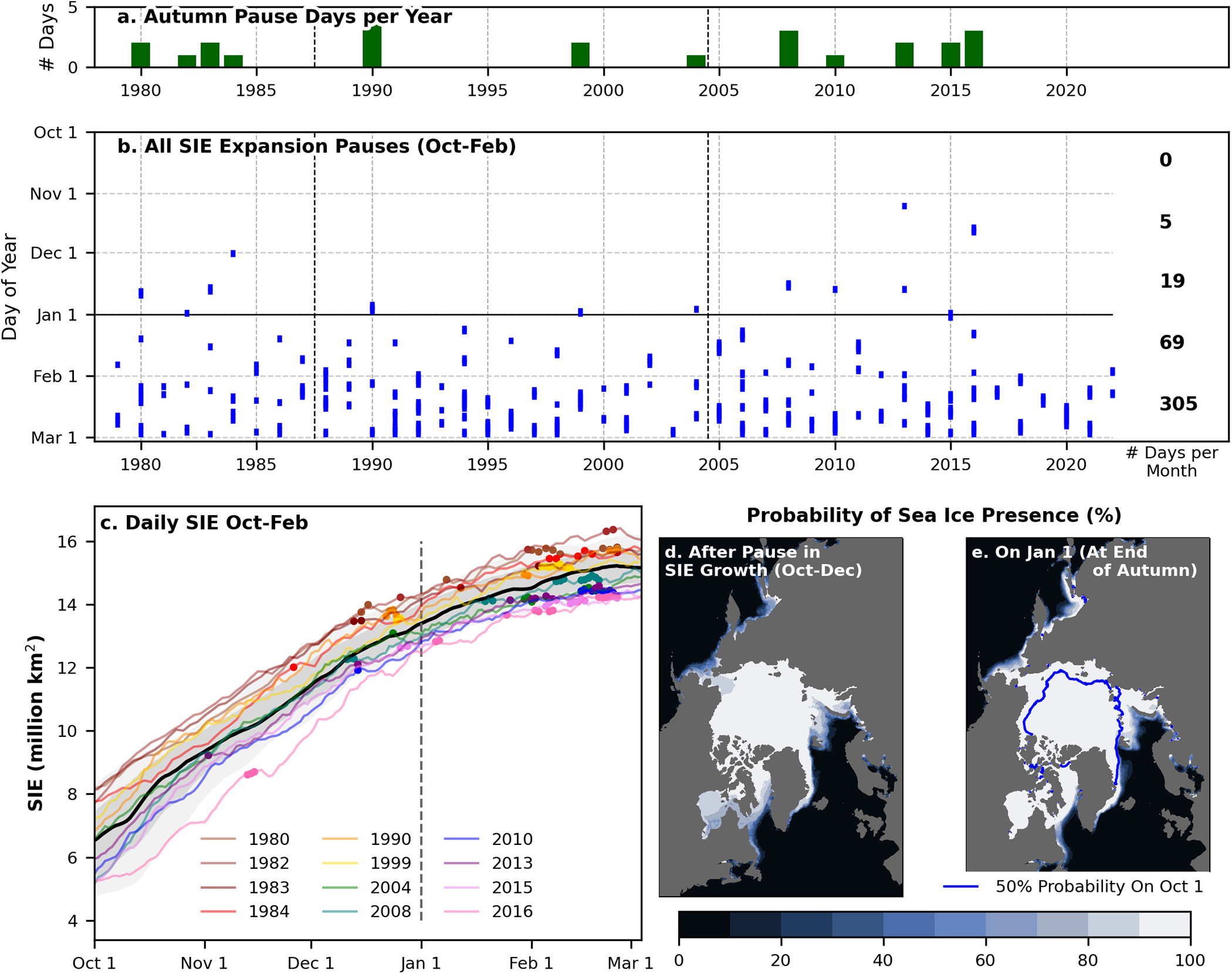
Pauses become more common as autumn progresses, with none occurring in October, 5 days (three events) occurring in November and 19 days (10 events) occurring in December. For comparison, 67 pause days (30 events) have occurred in January and 305 pause days (80 events) have occurred in February. This progression follows from the deceleration of SIE expansion that occurs throughout the growth season (Fig. 1c). As the expansion of SIE slows, pauses become more common, until the annual maximum SIE in late February or March. However, only 27% of years experience at least one pause event in autumn. Because of their greater rarity, SIE expansion pauses that occur in autumn (October–December) are the focus of this study.
3.2. Regional contributions
When pauses occur, the primary edge of Arctic sea ice typically lies in three main sectors (Fig. 1d, e): (1) the Nordic sector, comprising the Barents Sea, western Kara Sea and East Greenland Sea; (2) the Eastern Canada sector, comprising Hudson Bay, Baffin Bay and the Labrador Sea; and (3) the Pacific sector, comprising the southern Chukchi Sea, northern Bering Sea and coastal Sea of Okhotsk. The sea ice may also reside elsewhere, but it is consistently present in these three sectors (Fig. 2).
Regional characteristics of autumn Arctic SIE expansion pauses (1979–2022). (a) The 6 day change in SIE (∆SIE) for three key sectors during SIE expansion pauses. (b) Distribution of sectoral ∆SIE during autumn (box is the interquartile range, whiskers extend to 5th and 95th percentiles). (c) Relative frequency of autumn pauses in sectoral SIE expansion. (d) Sector definitions.
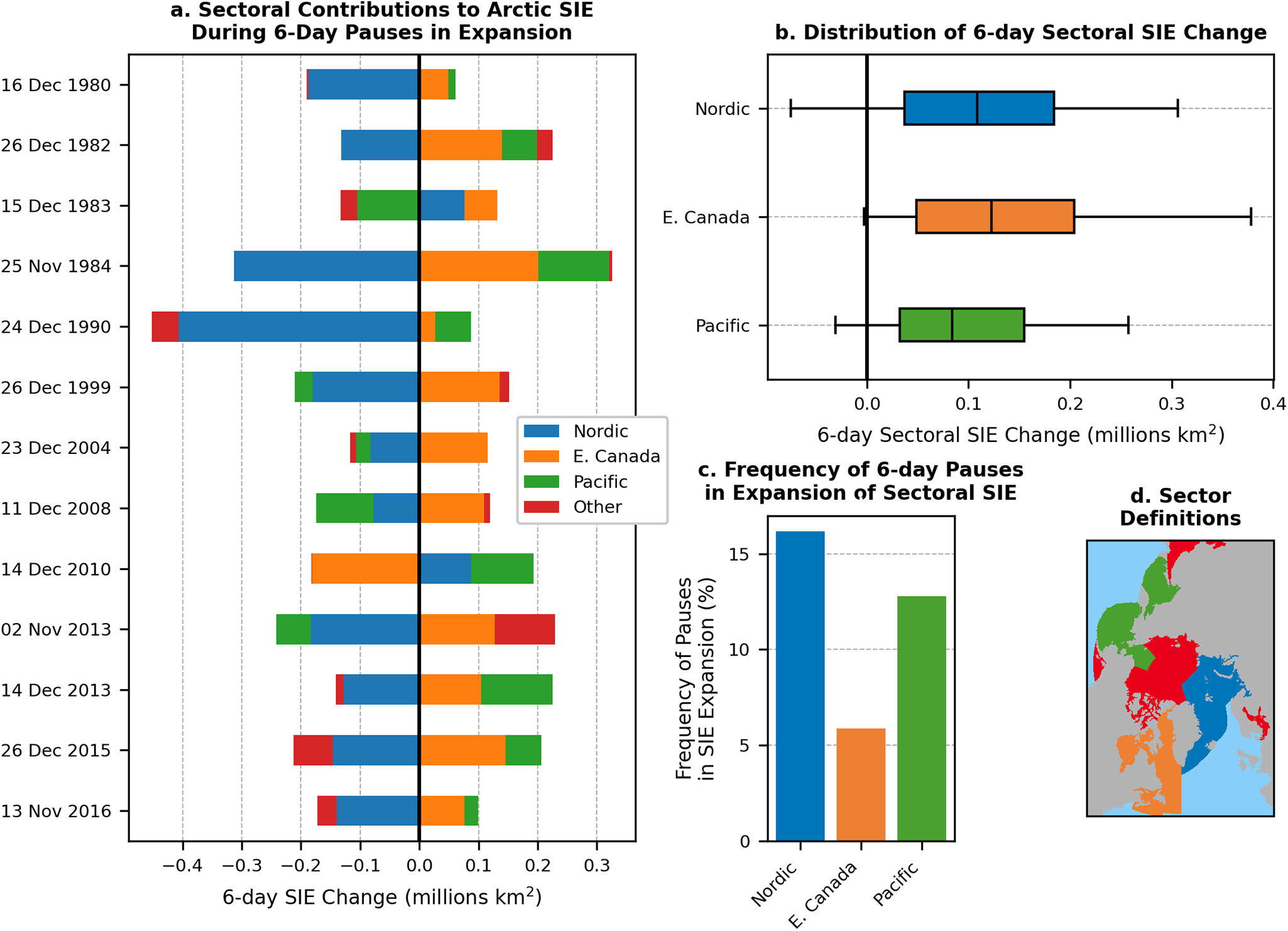
The Nordic sector is the most likely to experience a regional 6 day pause in autumn SIE growth (16% of autumn days); the Pacific sector is next most likely (12%); and the Eastern Canada sector is least likely (5%) (Fig. 2c). Of the 13 Arctic-wide SIE expansion pauses, 11 (85%) involved net sea-ice loss in the Nordic sector (Fig. 2a). This typically manifests as northward and/or westward retreat of the ice edge in the Barents and East Greenland Seas (Supplementary Fig. S2). Five SIE expansion pauses (38%) included net SIE loss in the Pacific sector, most notably 15 December 1983 and 11 December 2008 (Fig. 2a; Section 3.3.2). In another two Arctic-wide pause events, net SIE growth occurred in the Pacific sector, but much more slowly than average (Fig. 2b). During most pause events, the sea-ice edge sat in the Bering Sea and Sea of Okhotsk; however, the 2 November 2013 and 13 November 2016 events included retreat of the sea-ice edge in the southern Chukchi Sea (Supplementary Fig. S2).
In sharp contrast to the Nordic sector, the Eastern Canada sector exhibits net SIE growth during almost all Arctic-wide SIE expansion pauses (Fig. 2a). In fact, only the 14 December 2010 event involves net loss. During this event, the eastward advance of sea ice across Hudson Bay was stalled and reversed (Section 3.3.3). The December 2010 event is also notable as one of two that did not involve net sea-ice loss in the Nordic sector. Finally, other regions, like the central Arctic Ocean, have contributed only minorly to changes in SIE growth pauses in autumn (Fig. 1b). The most notable contribution from any of these ‘other’ regions was during the 2 November 2013 event (Fig. 1a), when a gap in sea-ice cover in the Amundsen Gulf of the Canadian Arctic Archipelago filled in, counteracting the pause (Supplementary Fig. S1).
3.3. Drivers of SIE expansion pauses
3.3.1. December 1990 and the primacy of the Nordic Seas
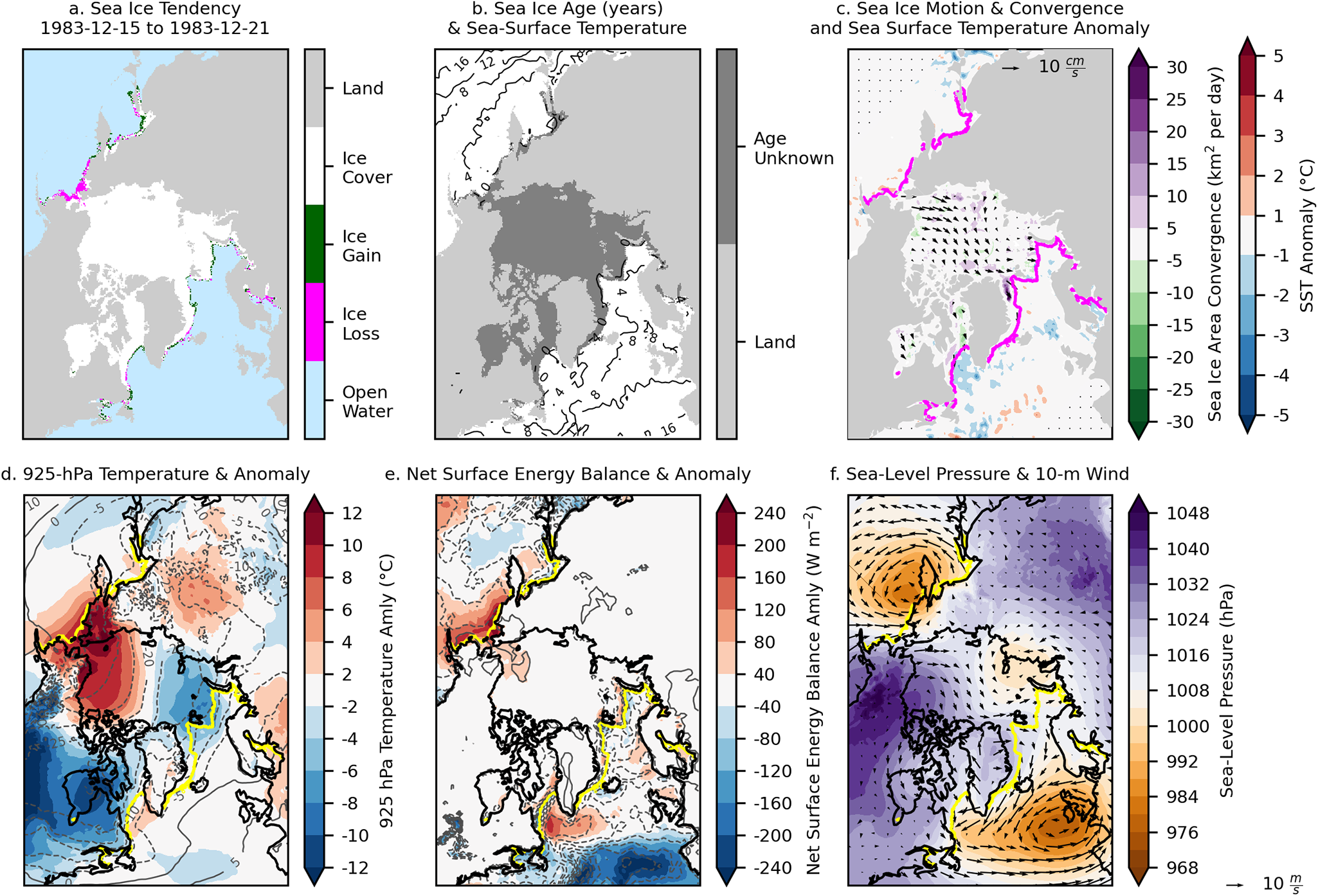
The greatest recorded 6 day decline in autumn SIE in the CDR occurred from 24 to 30 December 1990. SIE declined by 0.37 million km2 in the CDR, by 0.35 million km2 in the Bootstrap record (also the greatest decline), and by 0.20 million km2 in the NASA Team record (fourth greatest decline; Supplementary Fig. S3). The ∆SIE in the East Canada sector was positive, but well below average. In the Pacific sector, the ∆SIE was positive and only slightly below average. Therefore, this decline in SIE was primarily driven by exceptional loss in the Nordic sector (Fig. 2a). More specifically, loss occurred within a swath of first-year ice south and east of Svalbard and a swath of mixed first-year and multi-year ice in the East Greenland Sea and just north of Svalbard (Fig. 3a, b). The ice edge was pushed back 100–300 km in these regions.
The December 1990 SIE expansion pause. (a) Difference in SIE between 24 December 1990 and 30 December 1990. (b) Sea-ice age (shading; week 52) and sea surface temperature (contours with 4°C interval). (c) Sea-ice motion (vectors), sea-ice area convergence/divergence (purple/green shading), and sea surface temperature anomaly (red/blue shading). (d) 925 hPa air temperature (contours at 5°C interval) and anomaly (shading). (e) Surface energy balance anomaly (positive downward). (f) Mean sea-level pressure (shading) and 10 m wind (vectors). Anomalies are calculated with respect to the 35 day average centered on 24–30 December for the range of years 1981–2010.
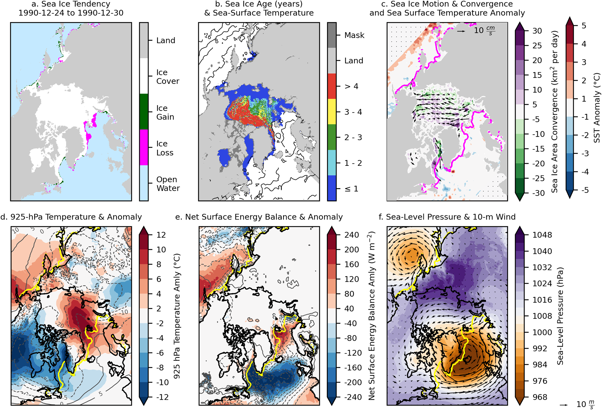
Sea-surface temperature was average for the time of year in the Nordic seas, but the atmosphere (at 925 hPa) was over 10°C warmer than average in a zone extending from Svalbard at the sea-ice edge all the way to the East Siberian Sea (Fig. 3c, d). The atmosphere was also warmer than average over the Sea of Okhotsk and the Bering Sea, and the surface energy balance exhibited positive anomalies as high as 200 W m−2 near Svalbard. However, the temperature was still sub-freezing, and surface energy balance was still upward (dashed contours in Fig. 3d and e, respectively) in all these regions. Therefore, the atmosphere was probably not inducing sea-ice melt.
Abnormal warmth was caused by southeasterly winds on the eastward flank of synoptic-scale cyclones, which were persistent enough to appear clearly in the 6 day average of mean sea-level pressure (Fig. 3f). In the Pacific sector, the winds were more easterly, running parallel to the sea-ice edge. However, in the Nordic sector, the winds blew perpendicular to the sea-ice edge, pushing it away from the Nordic Seas and causing convergence north of Greenland (Fig. 3c). In other words, the SIE expansion pause was primarily dynamical.
Extratropical cyclones are common in the Nordic Seas (Whittaker and Horn, Reference Whittaker and Horn1984; Gulev and others, Reference Gulev, Zolina and Grigoriev2001; Crawford and others, Reference Crawford, Schreiber, Sommer, Serreze, Stroeve and Barber2021), but late December 1990 stood out in two ways. First, four cyclones entered the East Greenland Sea over these six days (Supplementary Fig. S4). Second, three of the four cyclones were abnormally intense (Table 1). Compared to the maximum intensity for each autumn storm over the East Greenland/Barents Seas 1979–2023 (n = 1738), the first storm was below the 1st percentile of central sea-level pressure (933.4 hPa) and above the 99th percentile of pressure gradient (measured as the discrete difference of pressure at the center from the average pressure 1000 km away). Both lower central pressure and higher pressure gradient indicate a stronger storm. The second storm, a multicentered system, was at the 2nd percentile for central pressure and the 86th percentile for pressure gradient. The third storm, also a multicenter cyclone, was below the 1st percentile for pressure and at the 89th percentile for pressure gradient, which was strongest on its northeastern flank. The combination of three high-intensity storms taking similar tracks with tight temporal clustering led to the persistent cyclonic circulation that drove large and prolonged anomalies in temperature and wind.
Characteristics of extratropical cyclones associated with autumn SIE expansion pauses, including temporal clustering (multiple distinct storms following a very similar track) and the percentiles of the central pressure and pressure gradient (between center and a radius of 1000 km) for each storm, relative to other autumn storms in the given sector (October–December 1979–2023)
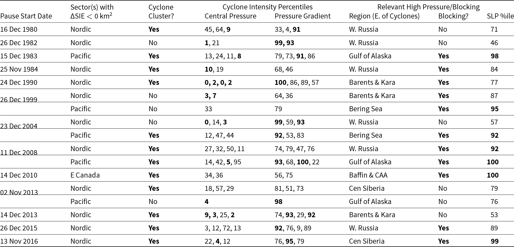
Also shown are the SLP percentile and presence of atmospheric blocking east of the extratropical cyclones (except north for 2010). Bold highlights extremes (above the 90th or below the 10th percentile).
When a strong pressure gradient exists, an extratropical cyclone may be just one half of the story. At the same time that the first and most intense of the cyclones passed through the East Greenland Sea, high pressure dominated over the Kara Sea, with average sea-level pressure at the 77th percentile. This high pressure coincided with a blocking event, as measured with 500 hPa geopotential height anomalies, that extended from Scandinavia and western Russia over the Barents and Kara Seas (Supplementary Fig. S4). The blocking helped keep the cyclones in East Greenland Sea, and therefore kept the Barents Sea on the receiving end of strong southeasterly winds.
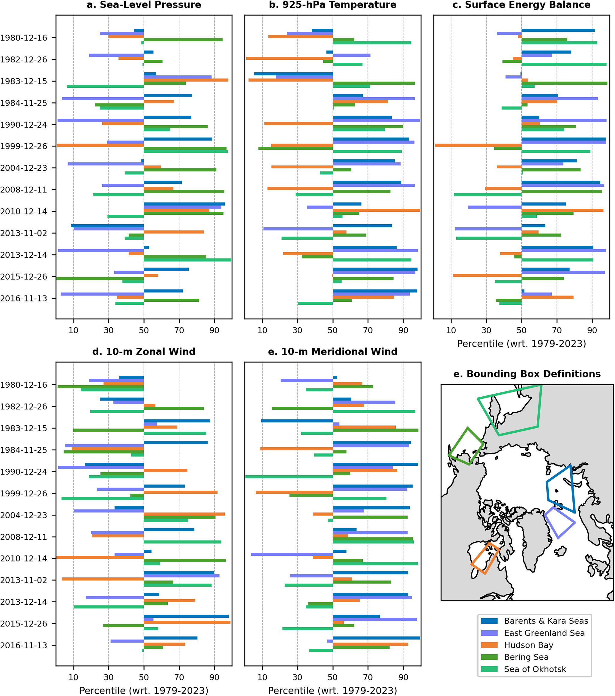
The example from December 1990 is the most extreme, but the atmospheric setup it exhibited is common to most SIE expansion pauses (Fig. 4; Supplementary Fig. S5). Those common characteristics include a series of abnormally strong extratropical cyclones passing through the East Greenland Sea (Table 1) that bring southerly winds to Svalbard and the Barents and Kara Seas, pushing the sea-ice edge poleward and inhibiting sea-ice growth by warming the atmosphere (although the 925 hPa temperature is still typically sub-freezing). Eleven out of 13 events in autumn involved below-median sea-level pressure over the East Greenland Sea. For six events, the sea-level pressure was below the tenth percentile. Ten out of 13 involved above-median 925 hPa air temperature over the Barents and Kara Seas, 12 of 13 involved above-median surface energy balance, and 12 of 13 involved southerly wind anomalies. Atmospheric blocking and anomalously high sea-level pressure to the east (over the Barents and Kara Seas or the adjacent continent), is also common, though not as common as anomalously intense extratropical cyclones in the East Greenland Sea (Table 1). Because of the connection to abnormal cyclone activity and blocking, we examined whether SIE expansion pauses are more likely during different phases of several seasonal (October–December) climate indices, including the Arctic Oscillation, North Atlantic Oscillation and Scandinavian Pattern, but no significant differences were found (Supplementary Table S2; p > 0.05 for a G-ratio test in all cases).
Percentiles from ERA5 for (a) sea-level pressure, (b) 925 hPa air temperature, (c) net surface energy balance and (d–e) 10 m wind velocity during the 13 pauses of at least 6 days in SIE expansion (ending on the listed dates) that occurred October–December. Parameters are spatially averaged for each region (e) and compared to the spatiotemporal averages for the same 6 day period 1979–2023 (1981–2023 for SST) as well as the two 6 day periods immediately before and after the event (meaning n ≥ 215 for percentile calculations). Bars pointing to the right indicate values above the median, and bars pointing to the left indicate values below the median.
3.3.2. December 1983: A Pacific Sector Event
A few exceptions to the typical Nordic-driven pattern exist. In two cases (15–21 December 1983 and 11–17 December 2008), sea-ice retreat in the Pacific sector—especially the Bering Sea—was a key reason for the Arctic-wide SIE expansion pause. During both the December 1983 and December 2008 events, the meridional wind anomaly and surface energy balance were over the 90th percentile in the Bering Sea—neither of which occurred during any other event (Fig. 4).
The 15–21 December 1983 event is the most interesting since it is one of only two pause events for which the Nordic sector experienced an increase in SIE (Fig. 2a). In fact, air temperature over the Barents and Kara Seas was ∼6–8°C below average, facilitating faster sea-ice growth than normal (Fig. 5d). Therefore, to pause Arctic-wide SIE growth, the Pacific sector needed an exceptional retreat. This event occurred in part because four separate intense extratropical cyclones migrated northeastward over the western Bering Sea over the course of 6 days (Supplementary Fig. S6). Using central pressure, they were the 13th, 24th, 11th and 8th percentiles (compared to other autumn storms in the Bering Sea or Sea of Okhotsk 1979–2023; Table 1). Similarly, using the pressure gradient, they were the 79th, 73rd, 91st and 86th percentiles—stronger than average, but not necessarily extreme. Their temporal clustering (likely encouraged by blocking in the Gulf of Alaska) and juxtaposition with extremely high sea-level pressure in the Gulf of Alaska (98th percentile; Table 1) maintained a targeted southerly atmospheric flow (Fig. 5f). This southerly flow, in turn, led to 925 hPa temperature anomalies exceeding 12°C (Fig. 5d). The 925 hPa temperature rose above 0°C as far north as 75°N in the Chukchi Sea on December 21 (not shown), and the surface energy balance reversed direction, suggesting that the sea ice in the northern Bering Sea was not just pushed poleward—it melted.
As in Figure 3, but for the December 1983 event (meaning week 50 for sea-ice age and 15–21 December 1983 for the temporal averaging). Note that no sea-ice age data are available for this event as the data product requires 5 consecutive years before producing a data product.
3.3.3. December 2010: An anticyclone and Hudson Bay
The final case study is the only Arctic-wide SIE expansion pause involving a regional decline of SIE in the Eastern Canada sector (Fig. 2a). The greatest sea-ice loss was within Hudson Bay, with notable loss in Baffin Bay as well (Fig. 6). The Pacific and Nordic sectors both experienced net gains in SIE.
As in Figure 3, but for the December 2010 event (meaning week 51 for sea-ice age and 14–20 December 2010 for the temporal averaging).
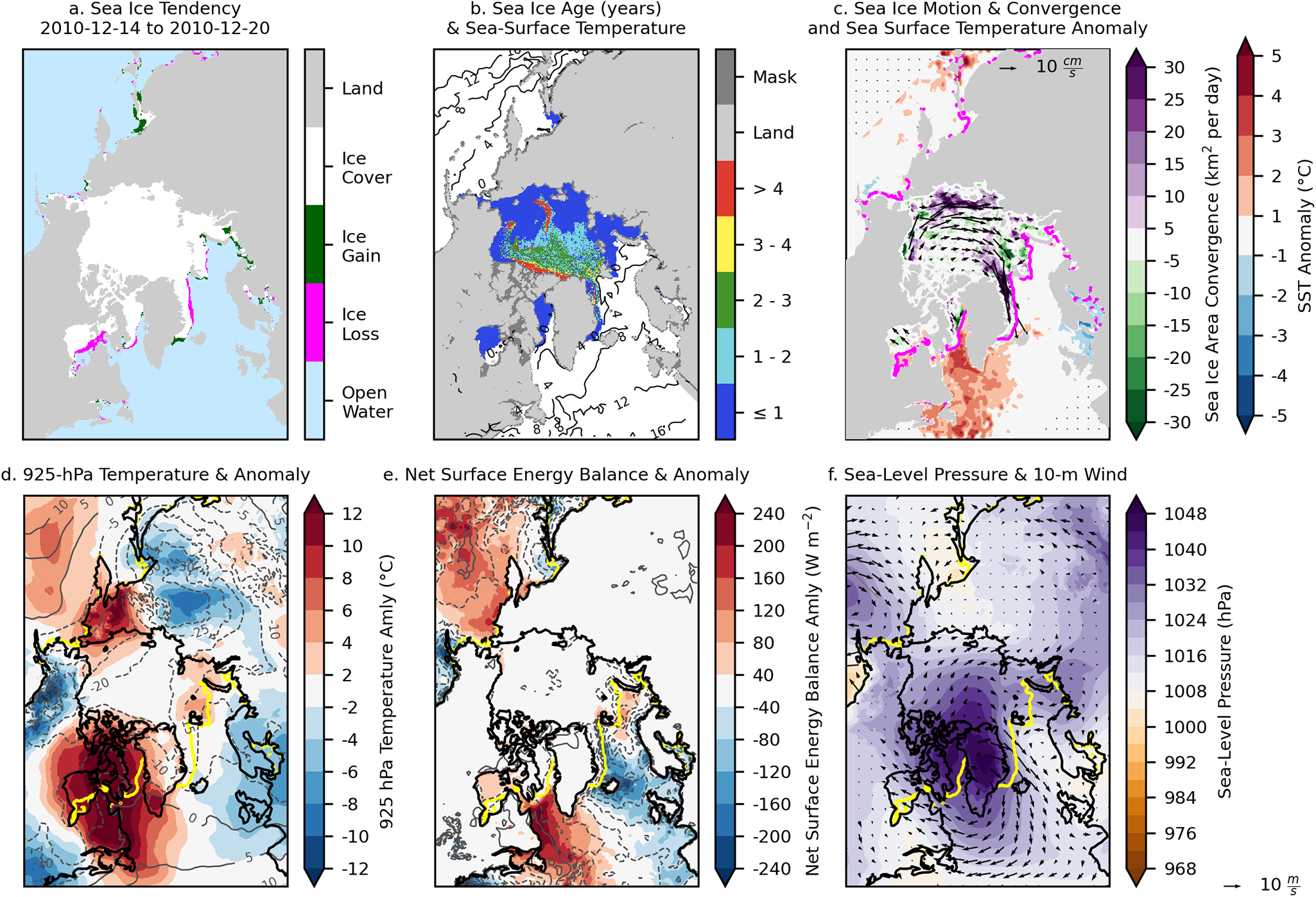
Most SIE expansion pauses can be attributed to a series of abnormally strong extratropical cyclones, but the December 2010 case relied instead on the strongest autumn anticyclone to ever occur over Baffin Bay region (65–80° N, 50–90° W) 1979–2023. The 6 day average sea-level pressure over the Baffin Bay region was a record 1043.0 hPa (Table 1). In the 500 hPa height, this feature appeared as a ridge that folded over the Canadian Arctic on 17 December and then was cut off by 20 December (Supplementary Fig. S7). Steering-level winds were therefore easterly (a reversal of the typical direction), and two extratropical cyclones moved east to west over southern Hudson Bay on 17 and 19 December. The storms were not exceptionally intense: 34th and 36th percentile by central pressure and 56th and 75th percentile by pressure gradient. Therefore, it was only when combined with the record-setting high to the north that these storms facilitated a unique circulation pattern for Hudson Bay: record-strength easterly 10 m winds, record-high 925 hPa temperatures, and a surface energy balance over the 95th percentile (Figs 4 and 6). Despite the temperature anomalies exceeding 12°C in places, the atmosphere was still below the melting point, and the surface energy balance was still negative, so as with most SIE expansion pauses, the sea-ice edge was not melting—it was being pushed back. In this case, that meant pushing the sea-ice edge westward.
Besides involving record high pressure, this event also involved notable timing. After sea-ice growth begins in northwestern Hudson Bay (usually in early November), it takes on average 20 days for sea ice to advance southeastward and cover the eastern side of the Bay (Crawford and others, Reference Crawford, Rosenblum, Lukovich and Stroeve2023). The record-strong easterly winds coincided with that 20 day window, so the ice in Hudson Bay was easier to break up and push back than if the ice were already piling against the islands and shoreline in eastern Hudson Bay. Sea ice advance into the eastern third of Hudson Bay did not occur until 2 January 2011—a record 4 weeks later than average (1979–2023).
3.4. SIE expansion pauses in a changing climate
3.4.1. Regimes shifts in Arctic sea ice
Pauses in autumn SIE expansion occur throughout the record, with no significant trend in frequency (p = 0.51 using Mann–Kendall test). The standard deviation of ∆SIE each autumn increased from 0.22 million km2 [6 days]−1 (1979–2004) to 0.26 million km2 [6 days]−1 (2005–22). Therefore, sea-ice growth is becoming more variable, but the change is best described as a regime shift from 2004 to 2005, not a steady trend (Fig. 7a).
SIE time series: (a) variability of SIE growth rate (within each autumn), (b) SIE on 1 October, (c) total autumn SIE growth, and (d) SIE on 1 January. Colored dots indicate the 12 years with an autumn SIE growth pause and horizontal dashed lines show average values for regimes detected using a Rodionov change-point analysis.

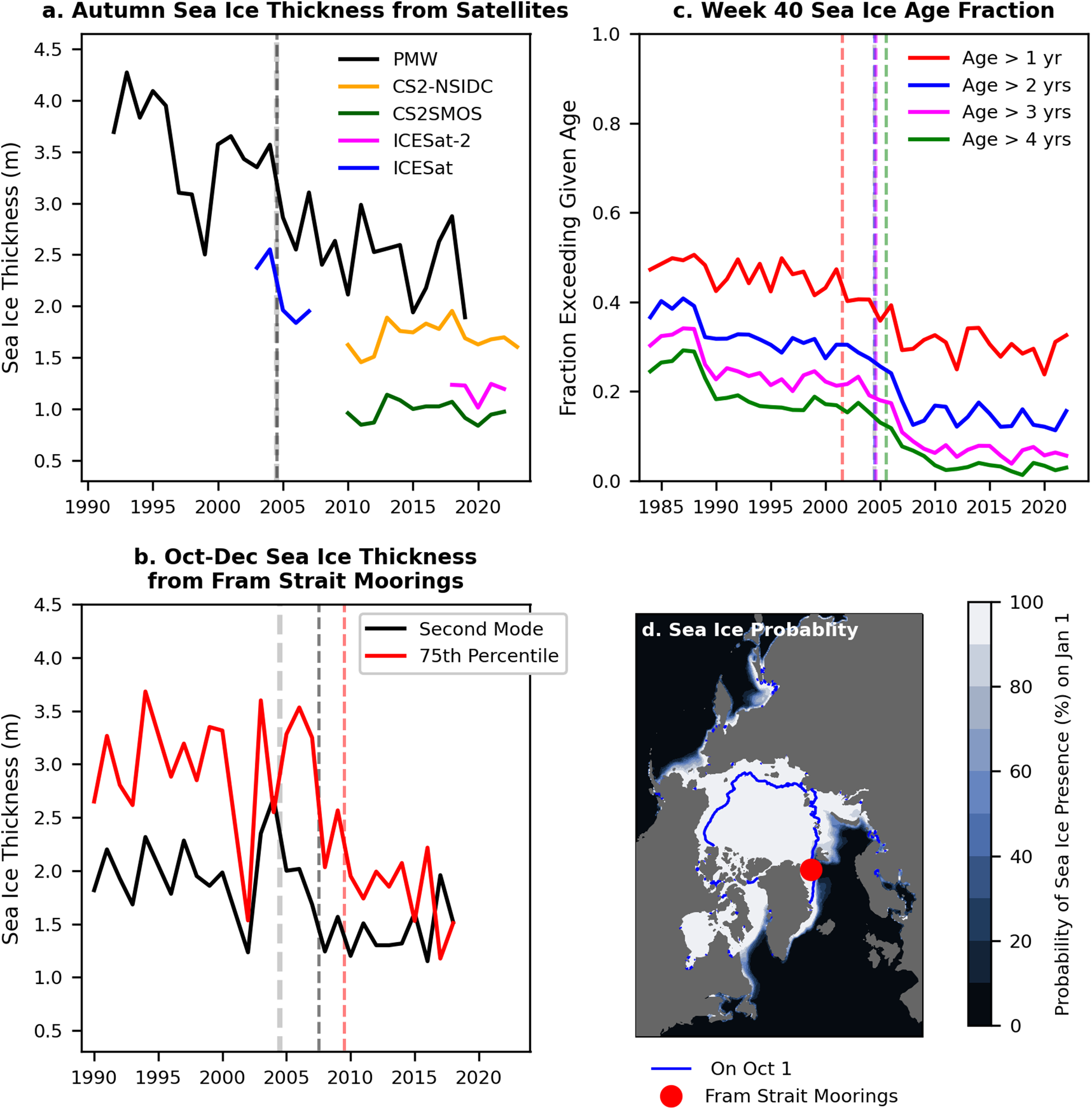
If we focus on sea ice in the area that is typically ice-covered on October 1, we find a decline in passive microwave-derived October–December ice thickness with a significant regime shift from 2004 to 2005 (p < 0.01 for Rodionov test; Fig. 8a). The IceSat thickness record also indicates a sharp drop from 2004 to 2005, and the later CryoSat-2 records shows no comparable drop 2010–22. The 2004–05 regime shift in ice thickness coincides with the significant regime shift for variability in ∆SIE, as well as a regime shift toward a lower fraction of sea ice aged over 2 years or over 3 years (p < 0.01 for Rodionov test; Fig. 8c). In other words, strong evidence exists that a regime shift toward thinner, younger sea ice starting in 2005 caused the regime shift in ∆SIE variability.
Annual time series of sea-ice thickness and age. (a) Satellite observations of average sea-ice thickness during October–December using passive microwave (PMW), CryoSat-2 (from NSIDC), CyroSat-2 + SMOS (from the Alfred Wegener Institute), and ICESat-2 or October–November using ICESat. (b) The second mode and 75th percentile of the thickness distribution measured by upward-looking sonar in Fram Strait during October-December. (c) Fraction in week 40 of each year (mid-October) that exceeds a given age (red line represents all multi-year ice). Averaging for (a) and (c) is conducted from grid cells that have at least a 50% probability of SIC > 15% on 1 October (blue outline in (d)). A wide, gray, vertical line between 2004 and 2005 indicates the regime shift for sea-ice total October–December growth and October–December ∆SIE.
If SIE expansion has become more variable, we would expect pauses in that expansion to become more common. This has not occurred, however, because the average autumn growth rate has also increased. SIE on 1 October has declined from ∼7.8 million km2 in 1979–98 to ∼5.4 million km2 2007–22 (Fig. 7b). SIE on 1 January has declined more modestly: from 14.3 million km2 1979–94 to 13.0 km2 2004–22 (Fig. 7d). Because the SIE on 1 October has declined by almost twice as much, the total growth of SIE from 1 October to 1 January each year has increased, with a marked shift from 2004 to 2005 (Fig. 7c). Therefore, the average ∆SIE has also increased (from 0.43 million km2 per 6 day period 1979–2004 to 0.50 million km2 per 6 day period 2005–22; p < 0.01). Since a pause in SIE expansion is defined as ∆SIE < 0 million km2, this change (in isolation) would make pauses in SIE expansion less common in the later period. When combined with a more variable growth rate resulting from thinner sea ice, the two effects cancel out, and pause events are about as common today as in the 1980s.
3.4.2. A minor role for changing weather extremes
Another factor that could impact ∆SIE variability and the occurrence of pauses in SIE expansion is change in its thermodynamic and dynamic drivers. One way to assess this is by examining the frequency of high and low extremes in atmospheric parameters before and after the 2004–05 regime shift. Since the Nordic sector is most important for driving pauses in seasonal SIE expansion (Section 3.2), the Barents/Kara and East Greenland Sea regions are of greatest interest.
The post-2004 period accounts for 42.2% of the record, so if extremes were evenly distributed through time, we would expect a similar fraction of both high extremes (above the 90th percentile) and low extremes (below the 10th percentile) to occur after 2004. Considering thermodynamics, extreme downward anomalies in surface energy balance became less common after 2004 in the Barents/Kara, East Greenland and Bering Sea regions (Fig. 9a), and upward extremes did not significantly change. If anything, this suggests the Nordic sector should be less susceptible to pauses in SIE expansion.
Percentage of 6 day atmospheric extremes occurring after 2004 by region in autumn. (a) Downward surface energy balance, (c) high sea-level pressure, (d) westerly wind and (g) southerly wind extreme anomalies are defined as the 90th percentiles, whereas (b) upward surface energy balance, (e) easterly wind, (f) low sea-level pressure and (h) northerly wind extremes are defined as the 10th percentiles. If extremes are equally likely before 2005 and after 2004, then 42.2% of all extremes are expected after 2004, so bars pointing to the right indicate more extremes in the later period than expected. Bootstrapping (with 1000 random selections) is used to calculate p-values (an x indicates a significantly disproportionate number of events after 2004).
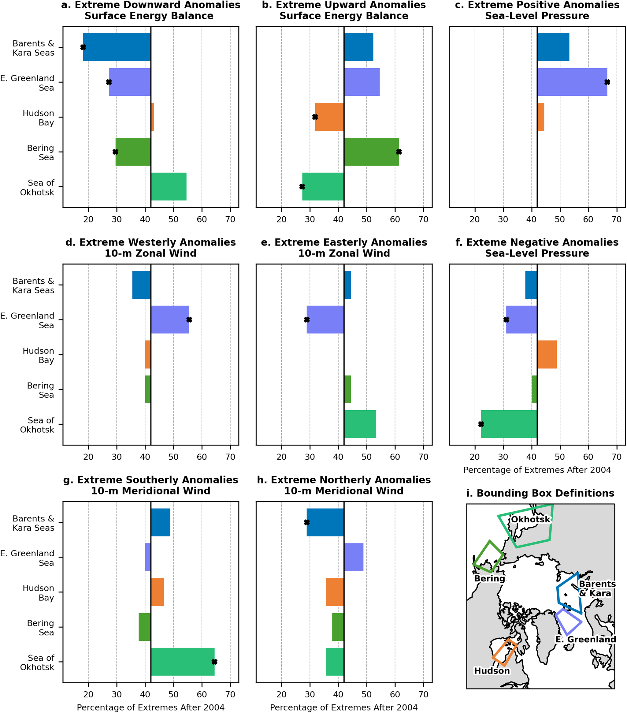
Considering dynamics, pauses in SIE expansion typically involve strong southerly and easterly wind anomalies in the Barents and Kara Seas, often driven by exceptional low pressure in the adjacent East Greenland Sea. Such extremes have not become more common, although extreme northerly wind anomalies in the Barents and Kara Seas have become less common. For the East Greenland Sea, extreme positive sea-level pressure and westerly wind anomalies have become more common. Such trends seem more likely to depress SIE expansion pauses than encourage them. However, there is no significant difference in the number of times ∆SIE < 0 km2 between 1979–2004 and 2005–22 in the Barents Sea (p = 0.17), Kara Sea (p = 0.36) or East Greenland Sea (p = 0.49).
The one region that does show signs of being more susceptible to pauses in SIE is the Sea of Okhotsk, with extreme upward surface energy balance anomalies becoming less common and extreme southerly wind anomalies becoming more common. Note that the Pacific Decadal Oscillation has also been more negative in October–December during the later period (median values of 0.22 for 1979–2004 and −1.02 for 2005–22; p = 0.01). A negative phase is correlated with southerly wind anomalies over the Sea of Okhotsk (Mantua and others, (Reference Mantua, Hare, Zhang, Wallace and Francis1997)). Accordingly, regional losses of SIE during October–December are more common since 2004 in the Sea of Okhotsk, with a median of 23.5 pause days per season 1979–2004 and 29 pause days per season 2005–22 (p < 0.01 from Mann–Whitney test). The Sea of Okhotsk differs from the Nordic Seas by its isolation from the central Arctic Ocean sea-ice pack, making changes to 1 October SIE, age or thickness in the central Arctic Ocean (Fig. 8) unimportant. In other words, it can operate independently.
4. Discussion and conclusions
4.1. Regional patterns and physical drivers
In a typical year, Arctic SIE exhibits uninterrupted growth in autumn (October–December). Pauses in growth (spanning at least 6 days) become more frequent in January and February as the average rate of SIE expansion slows and SIE nears its annual maximum. In autumn, however, only 13 pauses in SIE expansion occurred 1979–2022 (Fig. 1). We examined these 13 events, describing their regional patterns, physical drivers and response to climate change.
Pauses in autumn expansion of Arctic-wide SIE usually result from sea-ice loss in the Barents, Kara and East Greenland Seas (Fig 2). A common driver of these pauses is a series of extratropical cyclones moving into the East Greenland Sea, which produce a persistent low pressure anomaly and therefore southerly or southeasterly winds. These on-ice winds push the sea-ice edge backward to the north and west, temporarily stalling the seasonal expansion of SIE. They also bring warm, moist air poleward, weakening the upward transfer of energy from the surface to the atmosphere (Figs 3 and 4). Notably, though, the surface energy balance typically remains upward, suggesting that pauses in autumn SIE growth are primarily driven by dynamic loss, not melt.
One of these events (27 December 2015–1 January 2016) has was evaluated in detail using a combination of reanalysis and satellite data by Boisvert and others (Reference Boisvert, Petty and Stroeve2016). In addition to identifying that event as part of an Arctic-wide pause in SIE expansion, we also show that this atmospheric set-up is common to nearly all autumn pauses (Fig. 4). Ocean heat transport is also important to interannual variability of sea ice in the Barents Sea (Francis and Hunter, Reference Francis and Hunter2007; Koenigk and others, Reference Koenigk, Mikolajewicz, Jungclaus and Kroll2008; Efstathiou and others, Reference Efstathiou, Eldevik, Årthun and Lind2022), but we did not find consistent sea surface temperature anomalies during SIE expansion pauses, which are defined here as synoptic-scale events (e.g. Figs 3, 5 and 6). We focused on the direct impact of wind pushing sea ice in this paper, but the indirect impact of wind-driven waves that might break up the icepack (Asplin and others, Reference Asplin, Galley, Barber and Prinsenberg2012; Squire, Reference Squire2019) is also worth further consideration.
Another sector that is sometimes important for SIE expansion pauses is the Pacific, especially the southern Chukchi Sea, Bering Sea and Sea of Okhotsk. Previous work has noted how the winter ice edge in the Bering Sea is controlled by the location of the storm track associated with the Aleutian Low: SIE is lower when the storm track and Low are stronger and/or shifted to the west (Overland and Pease, (Reference Overland and Pease1982); Francis and Hunter, Reference Francis and Hunter2007). Again, ocean heat transport is also essential to understanding long-term trends (Zhang and others, Reference Zhang, Woodgate and Moritz2010; Wang and others, Reference Wang, Su, Jing and Guo2022). Best exemplified by the December 1983 event, we identified a persistent area of low pressure in the western Bering Sea and blocking and high pressure in the eastern Bering Sea or Gulf of Alaska as common drivers of Bering Sea-ice loss in autumn (Figs 4 and 5).
Our findings for atmospheric drivers of SIE pauses also share some properties with RILEs. Wang and others (Reference Wang, Walsh, Szymborski and Peng2020) describe a dipole pattern in geopotential height that induces a southerly flow of warm, moist air over regions that then experience rapid ice loss. We describe a similar pattern for pause events (Supplementary Figs 4–7), although our results emphasize the importance of not just one extremely strong cyclone, but often a series of cyclones of above-average strength clustered in time along a similar track, with the clustering often induced by blocking at the 500 hPa level (Table 1).
4.2. Explaining the lack of trends
We found no clear trend in the frequency of autumn SIE expansion pauses. If our definition of ‘pause’ were loosened to be ∆SIE < 0 km2 in any of the three products SIC products considered, 36 days in 21 events would qualify for inclusion instead of 24 days in 13 events. However, these extra days would be proportionally distributed in time, so there would still be no significant trend (p = 0.53).
The frequency of autumn sea-ice expansion pauses is affected by two compensatory trends: faster average growth discourages pauses, but more variable growth encourages pauses, leading to no trend in pause frequency. The negative feedback between larger ice-free areas in September and faster subsequent ice growth has been especially noticeable in the Kara and Laptev Seas (Zhang and others, Reference Zhang, Yi and Fan2024) and has led to an increase in rapid ice-growth events since 2005 (Stroeve and Notz, Reference Stroeve and Notz2018). This phenomenon is largely related to dynamic sea-ice growth, with the progressively thinning sea-ice pack (Fig. 8; Kwok, Reference Kwok2018; Babb, Reference Babb2023) being more mobile and moveable by winds and ocean currents (Ricker, Reference Ricker2017; Tandon and others, Reference Tandon, Kushner, Docquier, Wettstein and Li2018), including from extratropical cyclones (Schreiber and Serreze, Reference Schreiber and Serreze2020; Finocchio and others, Reference Finocchio, Doyle and Stern2022; Aue and Rinke, Reference Aue and Rinke2023). However, this added susceptibility to wind forcing also makes sea-ice growth more susceptible to the synoptic-scale variability in wind forcing.
Another sign that the increased variability in SIE growth rate stems from more mobile sea ice is that only in the Sea of Okhotsk is there a discernible increase in autumn atmospheric extremes likely to encourage sea-ice loss. In fact, in the Nordic sector, such extremes may be becoming less common (Fig. 9). Additionally, it may be notable that since the last autumn SIE expansion pause in 2016, sea-ice thickness in the Barents Sea has increased slightly, though not back to pre-2005 levels (Onarheim and others, Reference Onarheim, Årthun, Teigen, Eik and Steele2024). This may be making autumn pauses marginally less likely in the most recent years.
The regime shift in ∆SIE variability that occurred between 2004 and 2005 (Fig. 7a) aligns with a 2005 regime shift for central Arctic sea-ice thickness and age (Fig. 8), as well as Barents Sea-ice thickness (Onarheim and others, Reference Onarheim, Årthun, Teigen, Eik and Steele2024). However, 2007 is more often discussed as a key transition year for Arctic sea ice (e.g. Giles and others, Reference Giles, Laxon and Ridout2008; Livina and Lenton, Reference Livina and Lenton2013; Serreze and Meier, Reference Serreze and Meier2019; Babb, Reference Babb2023). The sea-ice thickness record from Fram Strait also does not show a regime shift in 2005, in disagreement with the passive microwave-derived record (Fig. 8c; Sumata and others, Reference Sumata, de, Divine, Granskog and Gerland2023). On the other hand, the increase in rapid ice-growth events identified by Stroeve and Notz (Reference Stroeve and Notz2018) occurred 2004–05, and Kwok (Reference Kwok2018) notes both 2005 and 2007 as years with major reductions in sea-ice thickness. The Fram Strait record is a more direct and fine-scale measure of sea-ice thickness than the passive microwave record product, but it is limited to sea ice passing through Fram Strait, whereas the main area of action for SIE expansion pauses is often to the east in the Barents and Kara Seas. The passive microwave record provides a more holistic view of Arctic Ocean sea-ice thickness, which may be why its regime shift better aligns with the shift in ∆SIE variability.
4.3. Conclusions
Arctic SIE does not always grow monotonically throughout autumn, and appreciating where, when, and why that growth pauses is an important component to understanding what matters to sub-seasonal sea-ice prediction. In this paper, we have shown that autumn pauses in SIE expansion are typically driven by temporal clusters of extratropical cyclones in the East Greenland Sea, which foster southerly or southeasterly winds that push back the ice edge and inhibit thermodynamic growth. Similar processes can also drive ice loss in the Pacific sector, but this is rarely sufficient on its own to cause an Arctic-wide SIE expansion pause. As summer SIE declines, autumn growth becomes faster on average, but a thinner ice pack is also more susceptible to atmospheric forcing. Therefore, even without changes to atmospheric extremes, SIE expansion pauses are likely to continue as rare but notable events in the next few decades. To project beyond that would require examination of output from climate model experiments. Finally, the frequency and patterns of SIE expansion pauses, like RILEs or rapid ice-growth events, could be used as evaluation metrics for sub-seasonal sea-ice forecasting models.
Supplementary material
The supplementary material for this article can be found at https://doi.org/10.1017/jog.2024.106.
Data availability statement
Datasets used in this study are openly available at the National Snow and Ice Data Center (DOIs for the SIC CDR: 10.7265/efmz-2t65; NASA Team SIC: https://doi.org/10.5067/MPYG15WAA4WX, Bootstrap SIC: 10.5067/X5LG68MH013O, IceSAT sea-ice thickness: https://doi.org/10.5067/1S5M59IQ0OK3, sea-ice age: https://doi.org/10.5067/UTAV7490FEPB, and sea-ice motion: https://doi.org/10.5067/INAWUWO7QH7B), Copernicus Climate Data Store (ERA5 DOI: https://doi.org/10.24381/cds.143582cf), Norwegian Polar Institute (Fram Strait sea-ice thickness DOI: https://doi.org/10.21334/npolar.2022.b94cb848), NOAA (sea surface temperature DOI: https://doi.org/10.1175/JCLI-D-20-0166.1; climate indices: https://www.ncei.noaa.gov/access/monitoring/pdo/, https://www.cpc.ncep.noaa.gov/products/precip/CWlink/daily_ao_index/teleconnections.shtml), or the Centre for Earth Observation Science (extratropical cyclone tracks DOI: https://doi.org/10.34992/ebnw-s681). Code to replicate data processing and figure creation is available at DOI: https://doi.org/10.5281/zenodo.4416124; processed data also available upon request.
Acknowledgements
J. Stroeve and C. Soriot were supported by the Canada C150 Program #50296. The authors thank Trevor Amestoy for help with the implementation of the Rodionov test in Python, Walt Meier for discussion about use of the NOAA/NSIDC CDR of SIC, and two anonymous reviewers for their comments.


 Open access