





1 Introduction
There has been an increasing interest in longitudinal data as they are powerful tools to track changes and development. In educational and psychological settings, one of the central topics is measuring individuals’ development of latent attributes over time. This is particularly important for assessing the effectiveness and impact of interventions on outcomes. Recently, hidden Markov models (HMMs) are becoming popular in psychology and education research as a method for modeling changes between attributes over time (Chen et al., Reference Chen, Culpepper, Wang and Douglas2018; Wang et al., Reference Wang, Yang, Culpepper and Douglas2018). HMMs are widely used in fields such as signal processing (Crouse et al., Reference Crouse, Nowak and Baraniuk2002) and information theory (Simola et al., Reference Simola, Salojärvi and Kojo2008) because of their ability to draw inferences about important unobservable states. In the context of educational and psychological testing, researchers have adapted the HMM framework to perform cognitive diagnosis using a class of models that will be referred to as restricted HMMs (RHMMs). RHMMs combine features of HMMs with a restricted latent class model (RLCM; Xu, Reference Xu2017), where the RLCM imposes structure on the emission probability—the conditional probability of a response given current hidden state. RHMMs, which integrate RLCM with HMM, along with the conventional HMMs have the potential to advance educational and psychological research, and help identify interventions that can enhance outcomes (Ye et al., Reference Ye, Fellouris, Culpepper and Douglas2016).
It is, thus, crucial to examine issues such as the identifiability conditions for these RHMMs to ensure accurate parameter recovery and reliable diagnostic inferences. Several studies have investigated the identifiability of HMMs (Allman et al., Reference Allman, Matias and Rhodes2009; Bonhomme et al., Reference Bonhomme, Jochmans and Robin2016), along with other research focusing on the identifiability of cognitive diagnostic models (CDMs; Xu, Reference Xu2017; Xu & Shang, Reference Xu and Shang2018) and RHMMs (Chen et al., Reference Chen, Liu, Xu and Ying2015, Reference Chen, Culpepper and Liang2020; Liu et al., Reference Liu, Culpepper and Chen2023). Methods for assessing model identifiability are applied under various conditions, as the structure of data can differ depending on the experimental designs, leading to different model specifications. Existing identifiability conditions for HMMs and RHMMs, which are derived under specific assumptions, may not be feasible in all settings. The focus of this article is to examine longitudinal settings (HMMs and RHMMs), evaluate existing model assumptions, and derive new identifiability results for different research designs that may be easier to satisfy in practice. Particularly, we examine three experimental designs: single-group pretest/posttest design, counterbalancing, and multiple-group longitudinal design.
The three experimental setups are used to evaluate the efficacy of interventions; however, each design relies on distinct assumptions which result in different modeling approaches. Motivation for choosing the three specified research designs comes from the following studies in the field of educational testing. Wang et al. (Reference Wang, Yang, Culpepper and Douglas2018) analyzed data from a counterbalancing study using a higher-order HMM combined with a constrained CDM. Their model assumes that once a student masters an attribute, they will never lose it. In contrast, Kaya and Leite (Reference Kaya and Leite2017) and Madison and Bradshaw (Reference Madison and Bradshaw2018a), in studies using single-group pretest/posttest design, allowed attribute levels to drop between two time points. The CDMs applied in Kaya and Leite (Reference Kaya and Leite2017), Madison and Bradshaw (Reference Madison and Bradshaw2018a), and Wang et al. (Reference Wang, Yang, Culpepper and Douglas2018) all require correct specification of a Q-matrix, a binary matrix that defines the relationships between the questions (e.g., test items) and the underlying attributes being measured. Similarly, Tang and Zhan (Reference Tang and Zhan2021) as well as Madison and Bradshaw (Reference Madison and Bradshaw2018b) developed models by integrating HMM with constrained CDMs for a study using a multiple-group longitudinal design. Tang and Zhan (Reference Tang and Zhan2021) allowed the item parameters at the first time point to be freely estimated while constraining those for later time points to ensure the comparability of item parameter estimates across groups and time points. On the other hand, the model proposed by Madison and Bradshaw (Reference Madison and Bradshaw2018b) can account for different item parameters between groups.
Recent advancements in existing software packages have allowed easier access for practitioners to estimate the parameters of RHMMs and apply the models (Madison et al., Reference Madison, Jeon, Cotterell, Haab and Zor2025). However, it should be noted that the RHMMs applied by Tang and Zhan (Reference Tang and Zhan2021), Madison and Bradshaw (Reference Madison and Bradshaw2018a, Reference Madison and Bradshaw2018b), Kaya and Leite (Reference Kaya and Leite2017), and Wang et al. (Reference Wang, Yang, Culpepper and Douglas2018) assume specific structures to the item responses and impose certain parameter constraints across items and attributes. Violations of these assumptions can result in inaccurate parameter estimates and misclassification of individual’s latent profiles. While these studies have significantly contributed to the development of methodologies for longitudinal designs, their focus was not on investigating model identifiability. There has been considerable research on identifiability of HMMs; however, few studies have extended these findings to RHMMs as used in the experimental designs discussed above. For instance, Liu et al. (Reference Liu, Culpepper and Chen2023) provide identifiability constraints for RHMMs with general RLCM and focus on situations where emission probabilities are formed using a deterministic inputs, noisy “and” gate (DINA; Junker & Sijtsma, Reference Junker and Sijtsma2001). The conditions derived by Liu et al. (Reference Liu, Culpepper and Chen2023) may apply to the single-group pretest/postest design, but may not extend to the other two experimental setups. Accordingly, the current work builds on existing research in identifying HMMs and RHMMs by specifying sufficient conditions for the remaining two designs: counterbalancing and multiple-group longitudinal designs.
In this article, we investigate HMMs with discrete time and finite observables and hidden states. Conventional HMMs consist of two components:
$1)$
 an emission matrix,
$\mathbf {B}$
an emission matrix,
$\mathbf {B}$
 , that describes the probability of observed responses given latent states and
$2)$
, that describes the probability of observed responses given latent states and
$2)$
 a transition matrix,
$\mathbf {A}$
a transition matrix,
$\mathbf {A}$
 , that denotes the likelihood of changing from one state to another over two adjacent time points. In existing identifiability research,
$\mathbf {B}$
, that denotes the likelihood of changing from one state to another over two adjacent time points. In existing identifiability research,
$\mathbf {B}$
 and
$\mathbf {A}$
and
$\mathbf {A}$
 are typically assumed to be constant over time along with an absence of an absorbing state. These requirements might not be satisfied depending on the research design employed and the associated assumptions. The two experimental setups examined in our article are situations where these specific assumptions might not be practical. Therefore, we want to relax these assumptions and impose other restrictions by considering HMMs with time-varying emission matrices as well as group-specific transition matrices. Based on the experimental designs, we provide new identification proofs for HMMs and RHMMs when
$\mathbf {B}$
are typically assumed to be constant over time along with an absence of an absorbing state. These requirements might not be satisfied depending on the research design employed and the associated assumptions. The two experimental setups examined in our article are situations where these specific assumptions might not be practical. Therefore, we want to relax these assumptions and impose other restrictions by considering HMMs with time-varying emission matrices as well as group-specific transition matrices. Based on the experimental designs, we provide new identification proofs for HMMs and RHMMs when
$\mathbf {B}$
 changes over time and
$\mathbf {A}$
changes over time and
$\mathbf {A}$
 differs between groups. The identifiability for HMMs discussed in our article is defined up to a permutation on the latent state labels. From the novel identifiability theorems, we demonstrate a Bayesian formulation and present a Gibbs sampling algorithm to estimate parameters for generalized HMMs in the case of the multiple-group longitudinal design. We demonstrate the flexibility and potential of our algorithms as well as the conventional HMMs through a data application designed to study the effectiveness of a learning intervention.
The remainder of the article is organized as follows. We first discuss existing HMM research in education and psychology in addition to introducing the typical setup of conventional HMMs and RHMMs. We then examine the counterbalancing and multiple-group longitudinal designs and generalize the results in Bonhomme et al. (Reference Bonhomme, Jochmans and Robin2016) to establish identifiability constraints. Next, we discuss how the new identifiability conditions may inform practitioners to design studies under HMM/RHMM framework. Afterward, we present a Bayesian formulation of generalized HMMs for the multiple-group longitudinal design and propose a Gibbs sampling algorithm for posterior approximation. The fifth section reports results of a Monte Carlo simulation study which illustrate the accuracy of the proposed algorithm. The algorithm is then applied to the dataset in Tang and Zhan (Reference Tang and Zhan2021) to demonstrate its ability to assess transitions between attributes in the evaluation of two interventions with respect to a control condition. The last section summarizes the findings of the present article and provides concluding remarks. All proofs and technical details are provided in the appendix.
2 Identifiability for HMM
This section examines identifiability conditions for three research designs: single-group pretest/posttest design, counterbalancing, and multiple-group longitudinal design. In a single-group pretest/posttest design, individuals complete evaluations before and after instruction, with both assessments typically using similar items. In contrast, counterbalancing and multiple-group longitudinal designs may involve more than two groups and varying items over time. We consider multiple-group longitudinal design to be experiments in which individuals are assigned to treatment and control groups. Performances are compared across groups, with the control group serving as the baseline, where minimal intervention occurs. Counterbalancing, on the other hand, involves administering a predetermined set of questions in different orders. The orders correspond to different test versions and participants are assigned to groups based on the test version they receive.
We begin the discussion on identifiability by presenting an overview of existing HMM research in education and psychology research. The first section also introduces the notation for conventional HMMs and the identifiability results from Liu et al. (Reference Liu, Culpepper and Chen2023) for the single-group pretest/postest design. Subsequent sections extend the definitions to the counterbalancing and multiple-group longitudinal designs, providing identifiability conditions for each. The last section provides comments and remarks on the general approach used to derive these conditions.
2.1 Overview of existing HMM research in education and psychology
Consider a general HMM model for an observation at time points
$t = 1, \ldots , T$
 . Let
$\boldsymbol {X} = (\boldsymbol {X}_1, \dots , \boldsymbol {X}_T)^\top \notag $
. Let
$\boldsymbol {X} = (\boldsymbol {X}_1, \dots , \boldsymbol {X}_T)^\top \notag $
 denote the response data of an individual over time. Let
$[q]$
denote the response data of an individual over time. Let
$[q]$
 for
$q\in \mathbb N$
for
$q\in \mathbb N$
 denote the set
$\{1, 2, \dots , q\}$
denote the set
$\{1, 2, \dots , q\}$
 . Here,
$\boldsymbol {X}_t = (X_{1t}, \dots , X_{Jt})$
. Here,
$\boldsymbol {X}_t = (X_{1t}, \dots , X_{Jt})$
 is the response pattern of an individual for J items at time t and
$\boldsymbol {X}_t \in ([M_1] \times [M_2] \times \dots \times [M_J])$
is the response pattern of an individual for J items at time t and
$\boldsymbol {X}_t \in ([M_1] \times [M_2] \times \dots \times [M_J])$
 . In other words,
$M_j$
. In other words,
$M_j$
 is the number of response options for an item j. Let
$\boldsymbol {Z} = (Z_1, \dots , Z_T)^\top \notag $
is the number of response options for an item j. Let
$\boldsymbol {Z} = (Z_1, \dots , Z_T)^\top \notag $
 be the latent states of an individual over time and
$Z_t \in [r]$
be the latent states of an individual over time and
$Z_t \in [r]$
 for
$r \in \mathbb {N}$
for
$r \in \mathbb {N}$
 . The response patterns
$\boldsymbol {X}_1, \ldots , \boldsymbol {X}_T$
. The response patterns
$\boldsymbol {X}_1, \ldots , \boldsymbol {X}_T$
 are assumed to be conditionally independent given
$Z_1, \ldots , Z_T$
are assumed to be conditionally independent given
$Z_1, \ldots , Z_T$
 . In other words, each
$\boldsymbol {X}_t$
. In other words, each
$\boldsymbol {X}_t$
 is directly impacted by the corresponding
$Z_t$
is directly impacted by the corresponding
$Z_t$
 and the conditional distribution is

Furthermore, within a first-order HMM, the distribution of
$Z_t$
 depends only on the previous state of the immediate past
$Z_{t - 1}$
depends only on the previous state of the immediate past
$Z_{t - 1}$
 . That is,

HMMs consist of two components. The first element is a transition matrix that dictates the likelihood of changing between latent states over two adjacent time points. Let
$\mathbf {A}$
 be an
$r \times r$
be an
$r \times r$
 transition matrix with each element
$(z_{t - 1}, z_{t})$
transition matrix with each element
$(z_{t - 1}, z_{t})$
 represents

which is the probability of transition to state
$Z_t = z_{t}$
 given the membership during the previous time is
$Z_{t - 1} = z_{t - 1}$
given the membership during the previous time is
$Z_{t - 1} = z_{t - 1}$
 . Observe that each element in
$\mathbf {A}$
. Observe that each element in
$\mathbf {A}$
 is non-negative and each row sums to one.
Additionally, there is an emission matrix that describes the distribution of observed responses given contemporaneous latent states. Let
$\mathbf {B}$
 be the
$q \times r$
be the
$q \times r$
 emission matrix with each element
$(\boldsymbol {x}_t, z_t)$
emission matrix with each element
$(\boldsymbol {x}_t, z_t)$
 denoted by

That is, each element in
$\mathbf {B}$
 represents the conditional probability of a response pattern given contemporaneous hidden state
$Z_t = z_t$
represents the conditional probability of a response pattern given contemporaneous hidden state
$Z_t = z_t$
 . The elements of
$\mathbf {B}$
. The elements of
$\mathbf {B}$
 are also non-negative and the columns sum to one.
We define
$\boldsymbol {\pi }_t = (\pi _{t, 1}, \ldots , \pi _{t, r}),$
 where
$\pi _{t, z_t}$
where
$\pi _{t, z_t}$
 is the probability of being in state
$Z_t = z_t$
is the probability of being in state
$Z_t = z_t$
 at time t. Then,
$\boldsymbol {\pi }_1$
at time t. Then,
$\boldsymbol {\pi }_1$
 is the initial distribution of the latent states. Observe that
$\sum _{z_t = 1}^r \pi _{t, z_t} = 1$
is the initial distribution of the latent states. Observe that
$\sum _{z_t = 1}^r \pi _{t, z_t} = 1$
 for any
$t \in [T]$
for any
$t \in [T]$
 . Using the initial distribution, we can iterate forward and find the distribution for time
$t = 2$
. Using the initial distribution, we can iterate forward and find the distribution for time
$t = 2$
 ,
$\boldsymbol {\pi }_2$
,
$\boldsymbol {\pi }_2$
 , to have elements

We can write
$\boldsymbol {\pi }_2 = \boldsymbol {\pi }_1 \mathbf {A}$
 . Consequently, iterating forward to time n implies that the distribution of latent states is
$\boldsymbol {\pi }_n = \boldsymbol {\pi }_1 \mathbf {A}^{n - 1}$
. Consequently, iterating forward to time n implies that the distribution of latent states is
$\boldsymbol {\pi }_n = \boldsymbol {\pi }_1 \mathbf {A}^{n - 1}$
 . The stationary (or long-run) distribution, which characterizes the marginal probability of residing in state
$z_t$
. The stationary (or long-run) distribution, which characterizes the marginal probability of residing in state
$z_t$
 , is defined as
$\boldsymbol {\pi } = \lim _{n \rightarrow \infty } \boldsymbol {\pi }_1 \mathbf {A}^n = (\pi _{1}, \ldots , \pi _{r})$
, is defined as
$\boldsymbol {\pi } = \lim _{n \rightarrow \infty } \boldsymbol {\pi }_1 \mathbf {A}^n = (\pi _{1}, \ldots , \pi _{r})$
 .
.
For HMMs and RHMMs, a model is identifiable when different values of the parameter set (
$\mathbf {A}, \mathbf {B}, \boldsymbol {\pi }_1$
 ) correspond to distinct marginal distributions of the observed variables. Model identifiability is essential for ensuring that the underlying parameters can be consistently estimated, thereby enabling the model to accurately assess the effects of interventions. Allman et al. (Reference Allman, Matias and Rhodes2009) provide a generic identifiability condition for HMMs using results in Kruskal (Reference Kruskal1977). More recently, Bonhomme et al. (Reference Bonhomme, Jochmans and Robin2016) establish sufficient conditions for identifying HMMs, which are more feasible to verify in practice.
Theorem 1 (Bonhomme et al., Reference Bonhomme, Jochmans and Robin2016).
Assume
$T \geq 3$
 . The matrices
$\mathbf {B}$
. The matrices
$\mathbf {B}$
 ,
$\mathbf {A}$
,
$\mathbf {A}$
 , and
$\mathbf {D}_{\boldsymbol {\pi }}$
, and
$\mathbf {D}_{\boldsymbol {\pi }}$
 are all identified if rank
$(\mathbf {B}) = r$
are all identified if rank
$(\mathbf {B}) = r$
 and rank
$(\mathbf {A}) = r$
and rank
$(\mathbf {A}) = r$
 , and
$\pi _r> 0$
, and
$\pi _r> 0$
 for all r
Here,
$\mathbf {D}_{\boldsymbol {\pi }} = \text {diag}(\pi _1, \dots , \pi _r)$
 . The proof of Theorem 1 involves rewriting HMMs into mixture models represented as three-way arrays, where the conditional distribution of the responses can be expressed in terms of
$\mathbf {B}$
. The proof of Theorem 1 involves rewriting HMMs into mixture models represented as three-way arrays, where the conditional distribution of the responses can be expressed in terms of
$\mathbf {B}$
 ,
$\mathbf {A}$
,
$\mathbf {A}$
 , and
$\boldsymbol {\pi }$
, and
$\boldsymbol {\pi }$
 . Then, Bonhomme et al. (Reference Bonhomme, Jochmans and Robin2016) derived conditions for finite HMMs to be identifiable using results from the simultaneous diagonalization problem (De Leeuw & Pruzansky, Reference De Leeuw and Pruzansky1978). It is worth noting that Theorem 1 applies to general HMMs and requires
$\mathbf {B}$
. Then, Bonhomme et al. (Reference Bonhomme, Jochmans and Robin2016) derived conditions for finite HMMs to be identifiable using results from the simultaneous diagonalization problem (De Leeuw & Pruzansky, Reference De Leeuw and Pruzansky1978). It is worth noting that Theorem 1 applies to general HMMs and requires
$\mathbf {B}$
 and
$\mathbf {A}$
and
$\mathbf {A}$
 to be full column rank. Other restrictions may be imposed to identify the parameters of an HMM. Liu et al. (Reference Liu, Culpepper and Chen2023) and Chen et al. (Reference Chen, Culpepper and Liang2020) extend the results to prove identifiability conditions for HMMs and RHMMs by relaxing some assumptions in Bonhomme et al. (Reference Bonhomme, Jochmans and Robin2016). Note that Liu et al. (Reference Liu, Culpepper and Chen2023) and Chen et al. (Reference Chen, Culpepper and Liang2020) focus on HMMs and RHMMs with binary latent attributes. Particularly, let K be the number of binary latent attributes, then the number of latent states is
$r = 2^K$
to be full column rank. Other restrictions may be imposed to identify the parameters of an HMM. Liu et al. (Reference Liu, Culpepper and Chen2023) and Chen et al. (Reference Chen, Culpepper and Liang2020) extend the results to prove identifiability conditions for HMMs and RHMMs by relaxing some assumptions in Bonhomme et al. (Reference Bonhomme, Jochmans and Robin2016). Note that Liu et al. (Reference Liu, Culpepper and Chen2023) and Chen et al. (Reference Chen, Culpepper and Liang2020) focus on HMMs and RHMMs with binary latent attributes. Particularly, let K be the number of binary latent attributes, then the number of latent states is
$r = 2^K$
 corresponding to all possible attribute profiles.
Theorem 2 (Liu et al., Reference Liu, Culpepper and Chen2023).
Let K be the total number of latent attributes. Consider the bipartition of all J items into two disjoint, nonempty subsets
$\mathbb {J}_1 = [S]$
 and
$\mathbb {J}_2 = \{S + 1, \dots , J\}$
and
$\mathbb {J}_2 = \{S + 1, \dots , J\}$
 . Then, rewrite
$\boldsymbol {X}_t = (\boldsymbol {X}^{\mathbb {J}_1 \top \notag }_t, \boldsymbol {X}^{\mathbb {J}_2 \top \notag }_t)$
. Then, rewrite
$\boldsymbol {X}_t = (\boldsymbol {X}^{\mathbb {J}_1 \top \notag }_t, \boldsymbol {X}^{\mathbb {J}_2 \top \notag }_t)$
 for
$t \in [T]$
for
$t \in [T]$
 . Let
$\mathbf {B}^{\mathbb {J}_1}$
. Let
$\mathbf {B}^{\mathbb {J}_1}$
 and
$\mathbf {B}^{\mathbb {J}_2}$
and
$\mathbf {B}^{\mathbb {J}_2}$
 be the emission matrices for
$\boldsymbol {X}^{\mathbb {J}_1}_t, \boldsymbol {X}^{\mathbb {J}_2}_t$
be the emission matrices for
$\boldsymbol {X}^{\mathbb {J}_1}_t, \boldsymbol {X}^{\mathbb {J}_2}_t$
 . We have
$\mathbf {B} = \mathbf {B}^{\mathbb {J}_1} \ast \mathbf {B}^{\mathbb {J}_2}$
. We have
$\mathbf {B} = \mathbf {B}^{\mathbb {J}_1} \ast \mathbf {B}^{\mathbb {J}_2}$
 , where
$\ast $
, where
$\ast $
 is the Khatri–Rao product defined in Definition A.2 in Appendix A. The parameters are identifiable if rank
$(\mathbf {A}) = 2^K$
is the Khatri–Rao product defined in Definition A.2 in Appendix A. The parameters are identifiable if rank
$(\mathbf {A}) = 2^K$
 ,
$\pi _l> 0$
,
$\pi _l> 0$
 for all l, and
-
(a) for $T \geq 3$
 , rank
$\!(\mathbf {B}) = 2^K$
;
, rank
$\!(\mathbf {B}) = 2^K$
; -
(b) for $T = 2$
, rank
$\!(\mathbf {B}^{\mathbb {J}_1}) = 2^K$
and rank
$\!_K(\mathbf {B}^{\mathbb {J}_2}) \geq 2$
.


Note rank
$_K$
 in part (b) of Theorem 2 denotes the Kruskal rank. The Kruskal rank of a matrix with r columns equals r if and only if the matrix has full column rank (see Definition A.1 in Appendix A for more details). Moreover, observe that certain assumptions are shared between Theorems 1 and 2. Namely,
$\mathbf {B}$
in part (b) of Theorem 2 denotes the Kruskal rank. The Kruskal rank of a matrix with r columns equals r if and only if the matrix has full column rank (see Definition A.1 in Appendix A for more details). Moreover, observe that certain assumptions are shared between Theorems 1 and 2. Namely,
$\mathbf {B}$
 as well as
$\mathbf {A}$
as well as
$\mathbf {A}$
 need to be constant over time, and that every element of the stationary distribution is positive. We now examine what these assumptions entail in real-world settings as well as within the model.
2.2 Challenges with current HMMs
Bonhomme et al. (Reference Bonhomme, Jochmans and Robin2016), Chen et al. (Reference Chen, Culpepper and Liang2020), and Liu et al. (Reference Liu, Culpepper and Chen2023) assume
$\mathbf {B}$
 and
$\mathbf {A}$
and
$\mathbf {A}$
 to be time invariant along with every element in
$\boldsymbol {\pi }$
to be time invariant along with every element in
$\boldsymbol {\pi }$
 to be positive. It is essential to understand the implications of these assumptions. Having constant
$\mathbf {B}$
to be positive. It is essential to understand the implications of these assumptions. Having constant
$\mathbf {B}$
 implies that the conditional distribution
$P(\boldsymbol {X}_t \mid Z_t)$
implies that the conditional distribution
$P(\boldsymbol {X}_t \mid Z_t)$
 does not change with time. In other words, parallel measurements are observed across different time points. This assumption could be reasonable when a common set of items is used over time, such as diagnosing mental health conditions with a standardized questionnaire. However, the constant
$\mathbf {B}$
does not change with time. In other words, parallel measurements are observed across different time points. This assumption could be reasonable when a common set of items is used over time, such as diagnosing mental health conditions with a standardized questionnaire. However, the constant
$\mathbf {B}$
 assumption is not always feasible, such as when there may be item parameter drift or when different items are administered over time.
The assumption of constant
$\mathbf {A}$
 suggests that
$P(Z_t \mid Z_{t - 1})$
suggests that
$P(Z_t \mid Z_{t - 1})$
 remains the same for all t. That is, the process being modeled is assumed to be stable during the observation period. This assumption is possible when data are collected over a short time span and conditions are expected to remain consistent. However, the constant
$\mathbf {A}$
remains the same for all t. That is, the process being modeled is assumed to be stable during the observation period. This assumption is possible when data are collected over a short time span and conditions are expected to remain consistent. However, the constant
$\mathbf {A}$
 assumption may be violated in studies involving extended periods or heterogeneous populations, where individual response to interventions may vary. For example, in educational settings, learning interventions may only be effective for certain subgroups, resulting in different transition dynamics between the groups.
The last assumption requires
$\boldsymbol {\pi }> \boldsymbol {0}_r$
 with
$\boldsymbol {0}_r$
with
$\boldsymbol {0}_r$
 represents an r-vector of zeros and “
$>$
represents an r-vector of zeros and “
$>$
 ” is an element-wise inequality. This pertains to the irreducibility of
$\mathbf {A}$
” is an element-wise inequality. This pertains to the irreducibility of
$\mathbf {A}$
 , which is violated if
$\mathbf {A}$
, which is violated if
$\mathbf {A}$
 contains absorbing states. A state
$z_{t - 1}$
contains absorbing states. A state
$z_{t - 1}$
 is an absorbing state if it has a
$100\%$
is an absorbing state if it has a
$100\%$
 of transitioning to itself and
$0\%$
of transitioning to itself and
$0\%$
 to any other states. Intuitively, an absorbing state is a state such that once entered, cannot be left. The irreducibility assumption can be violated in educational research aimed at learning advancement. In such cases, interventions are designed to enhance skill development toward a mastery state, which may function as an absorbing state if skill forgetting is considered unlikely.
For a single-group pretest/posttest design, the assumptions of constant
$\mathbf {B}$
 and
$\mathbf {A}$
and
$\mathbf {A}$
 are often reasonable as it is common to use similar assessments before and after an intervention. Consider a study in mathematics education examining the effects of the Enhanced Anchored Instruction program (Bottge et al., Reference Bottge, Heinrichs, Chan, Mehta and Watson2003) on mathematics achievement of middle school students (Li et al., Reference Li, Cohen, Bottge and Templin2016). The study investigates the impact of the EAI intervention by observing student’ performance on a test called fraction of the cost (FOC). The same FOC test is administered before and after the intervention. Hence, we can see that the constant
$\mathbf {B}$
are often reasonable as it is common to use similar assessments before and after an intervention. Consider a study in mathematics education examining the effects of the Enhanced Anchored Instruction program (Bottge et al., Reference Bottge, Heinrichs, Chan, Mehta and Watson2003) on mathematics achievement of middle school students (Li et al., Reference Li, Cohen, Bottge and Templin2016). The study investigates the impact of the EAI intervention by observing student’ performance on a test called fraction of the cost (FOC). The same FOC test is administered before and after the intervention. Hence, we can see that the constant
$\mathbf {B}$
 and
$\mathbf {A}$
and
$\mathbf {A}$
 assumptions are satisfied here. Furthermore, the study consists of only two time points, making the likelihood of having a complete mastery state to be unlikely. This means that students can be expected to obtain or retain knowledge as well as forget some knowledge over the short periods. Therefore, the irreducibility assumption is also feasible, allowing Theorem 2 to be applied to this design. However, these assumptions may not hold for situations where item parameters change over time and there are multiple groups with heterogeneous transition parameters. The next sections discuss the specific setups and identifiability proofs of two designs that we recommend using in cases where item parameters differ over time or when there are known groups that might differ in the probability of achieving mastery.
2.3 Counterbalancing for longitudinal diagnostic design
There are several advantages for one to consider implementing a counterbalancing design. This design balances out the item positions and controls for potential order effects. Wang et al. (Reference Wang, Yang, Culpepper and Douglas2018) proposed using a counterbalanced booklet design to address confounding factors that could obscure learning effects. Additionally, Wang et al. (Reference Wang, Yang, Culpepper and Douglas2018) noted that counterbalancing can help avoid empirical identifiability issues associated with using RLCMs, specifically the DINA model. Particularly, they provided the example of estimated guessing parameters being inaccurate for items in later time points. This can happen when there is no guessing because all individuals within a sample have mastered the required attributes by the time they get to the items. Nevertheless, the primary aim of Wang et al. (Reference Wang, Yang, Culpepper and Douglas2018) was not to understand the identifiability of HMMs. The current article fills this gap by formally deriving identifiability conditions for RHMMs under a counterbalancing design.
In what we refer to as a counterbalancing design, a fixed number of questions are arranged into different orderings. These orderings correspond to the various versions of the test, and examinees are then categorized into groups depending on the version they receive. That is, counterbalancing here refers to an experimental design in which the same set of items is administered in different orders across examinees to control for potentially confounding factors, such as order and time effects. This design is relatively popular in both classroom and large-scale assessments (Johnson, Reference Johnson1992; Shute et al., Reference Shute, Hansen and Almond2008). While counterbalancing can be implemented in many ways, we focus only on those configurations that are relevant for ensuring model identifiability, which will be specified later in this article. An example is the experiment conducted by Wang et al. (Reference Wang, Yang, Culpepper and Douglas2018), where participants responded to 50 items organized into five 10-item blocks, with a learning intervention administered between blocks. Here, the five equal-size partitions of the 50 items are referred to as booklets 1–5. Counterbalancing was implemented by rotating each of the five booklets to be administered first in the sequence (Table 1).
Balanced block design in Wang et al. (Reference Wang, Yang, Culpepper and Douglas2018)

Table 1 Long description
The table consists of six columns and six rows. The first row contains the header Time points, spanning columns two through six, labeled 1, 2, 3, 4, and 5. The first column lists the Groups from 1 to 5.
Row 2 (Group 1): Time 1 is Booklet 1, Time 2 is Booklet 2, Time 3 is Booklet 3, Time 4 is Booklet 4, Time 5 is Booklet 5.
Row 3 (Group 2): Time 1 is Booklet 2, Time 2 is Booklet 3, Time 3 is Booklet 4, Time 4 is Booklet 5, Time 5 is Booklet 1.
Row 4 (Group 3): Time 1 is Booklet 3, Time 2 is Booklet 4, Time 3 is Booklet 5, Time 4 is Booklet 1, Time 5 is Booklet 2.
Row 5 (Group 4): Time 1 is Booklet 4, Time 2 is Booklet 5, Time 3 is Booklet 1, Time 4 is Booklet 2, Time 5 is Booklet 3.
Row 6 (Group 5): Time 1 is Booklet 5, Time 2 is Booklet 1, Time 3 is Booklet 2, Time 4 is Booklet 3, Time 5 is Booklet 4.
The design follows a Latin Square pattern where each booklet appears exactly once in each group and once at each time point.
Following the experimental setup of Wang et al. (Reference Wang, Yang, Culpepper and Douglas2018), this article focuses on the case with binary response data, but the proof can be extended to the case where items are polytomous. The remainder of this section introduces the RHMM framework and presents a new identifiability theorem for RHMMs specific to the counterbalancing design.
2.3.1 General model
Let there be G total groups where each group corresponds to a unique ordering of the booklets. Observe that, for a given time point, two groups may have different booklets. That is, examinees from separate groups may answer multiple different items at varying time points, resulting in different responses. In the HMM framework, this implies that the emission matrix
$\mathbf {B}$
 may change over time and we can define the multi-item emission matrix.
Definition 1 (Multi-item emission matrix).
Suppose there are J total items with
$M_j$
 representing the number of response options for item j. Let
$\mathbb {J}_t \subset [J]$
representing the number of response options for item j. Let
$\mathbb {J}_t \subset [J]$
 to be the set of items administered at time t. The emission matrix of an item is defined as

and the emission matrix at time t is

where
$\mathop {{{{\circledast }}}}_{j \in \mathbb J_t}$
 denotes the Khatri–Rao product (i.e., a column-wise Kronecker product) of matrices
$\mathbf {B}_j$
denotes the Khatri–Rao product (i.e., a column-wise Kronecker product) of matrices
$\mathbf {B}_j$
 for all
$j \in \mathbb J_t$
for all
$j \in \mathbb J_t$
 (see Definition A.3 in Appendix A).
Let K be the total number of binary latent attributes and J be the total number of items. The conditional distribution of the response
$\boldsymbol {X}$
 in the emission matrix is written in terms of
$\boldsymbol {\alpha } \in \{0, 1\}^K$
in the emission matrix is written in terms of
$\boldsymbol {\alpha } \in \{0, 1\}^K$
 , as opposed to
$\boldsymbol {Z}$
, as opposed to
$\boldsymbol {Z}$
 . That is, for the remainder of this section on counterbalancing, the number of latent states is
$r = 2^K$
. That is, for the remainder of this section on counterbalancing, the number of latent states is
$r = 2^K$
 corresponding to all possible attribute profiles. Here,
$\boldsymbol {\alpha } = (\boldsymbol {\alpha }_1, \dots , \boldsymbol {\alpha }_T)^\top \notag $
corresponding to all possible attribute profiles. Here,
$\boldsymbol {\alpha } = (\boldsymbol {\alpha }_1, \dots , \boldsymbol {\alpha }_T)^\top \notag $
 denotes the learning trajectory of individual i, where
$\boldsymbol {\alpha }_t = (\alpha _{1t}, \dots , \alpha _{Kt})$
denotes the learning trajectory of individual i, where
$\boldsymbol {\alpha }_t = (\alpha _{1t}, \dots , \alpha _{Kt})$
 represents the binary attribute profile at time t. The element
$\alpha _{kt} = 1$
represents the binary attribute profile at time t. The element
$\alpha _{kt} = 1$
 indicates that the respondent possesses attribute k for
$k \in [K]$
indicates that the respondent possesses attribute k for
$k \in [K]$
 , and
$\alpha _{kt} = 0$
, and
$\alpha _{kt} = 0$
 otherwise. When the items are dichotomous, the emission probability conditional on the attribute profile
$\boldsymbol {\alpha }_t$
otherwise. When the items are dichotomous, the emission probability conditional on the attribute profile
$\boldsymbol {\alpha }_t$
 is
is

where
$\boldsymbol {\Omega }$
 represents the model parameters,
$\mathbb {J}_t$
represents the model parameters,
$\mathbb {J}_t$
 denotes the set of items administered at time t with elements denoted by
$\mathbb {j}_1,\dots , \mathbb {j}_{|\mathbb J_t|}$
denotes the set of items administered at time t with elements denoted by
$\mathbb {j}_1,\dots , \mathbb {j}_{|\mathbb J_t|}$
 , and
$b_{j, x_t, \boldsymbol {\alpha }_t}$
, and
$b_{j, x_t, \boldsymbol {\alpha }_t}$
 is an element of an item-specific matrix, which denotes the probability of a response
$x_t$
is an element of an item-specific matrix, which denotes the probability of a response
$x_t$
 to item j at time t for a subject with attribute profile
$\boldsymbol {\alpha }_t$
to item j at time t for a subject with attribute profile
$\boldsymbol {\alpha }_t$
 .
.
Equation (1) is a general form of the emission probability that contains the response probabilities for all
$2^K$
 latent classes for each item. The current model is unrestricted in the sense that there are no constraints on the emission probabilities. This lack of constraint, however, makes the general model susceptible to the label switching problem, a well-known issue in latent class modeling (Jasra et al., Reference Jasra, Holmes and Stephens2005; Redner & Walker, Reference Redner and Walker1984). Specifically, across different groups and time points, the latent classes associated with the items can vary in order or even differ entirely. However, this problem is mitigated in RHMMs, where some structure is introduced by an expert-specified
$\boldsymbol {Q}$
latent classes for each item. The current model is unrestricted in the sense that there are no constraints on the emission probabilities. This lack of constraint, however, makes the general model susceptible to the label switching problem, a well-known issue in latent class modeling (Jasra et al., Reference Jasra, Holmes and Stephens2005; Redner & Walker, Reference Redner and Walker1984). Specifically, across different groups and time points, the latent classes associated with the items can vary in order or even differ entirely. However, this problem is mitigated in RHMMs, where some structure is introduced by an expert-specified
$\boldsymbol {Q}$
 matrix (see below) and imposed on the emission matrix.
The restrictions can be connected to alternative representations where CDMs are written as a mixture of generalized linear models (de la Torre, Reference de la Torre2011; Henson et al., Reference Henson, Templin and Willse2009; von Davier, Reference von Davier2008). The response probability for an item j is now modeled as

where
$\Psi (\cdot )$
 is an arbitrary cumulative distribution function,

is an alternative form of the binary vector
$\boldsymbol {\alpha }_{t}$
 , and
, and

The regression coefficients create a sparse vector
$\boldsymbol {\beta }_{j}$
 , where the nonzero elements represent the effects of latent skills or combination of skills on the response of item j. It can be shown that CDMs can be reparameterized to Equation (2) with different sparsity patterns of the vector
$\boldsymbol {\beta }_{j}$
, where the nonzero elements represent the effects of latent skills or combination of skills on the response of item j. It can be shown that CDMs can be reparameterized to Equation (2) with different sparsity patterns of the vector
$\boldsymbol {\beta }_{j}$
 . Following notations from Chen et al. (Reference Chen, Culpepper and Liang2020), let
$\boldsymbol {\delta }_j = (\delta _{j0},\dots ,\delta _{j,2^K-1})^\top \notag \in \{0, 1\}^{2K}$
. Following notations from Chen et al. (Reference Chen, Culpepper and Liang2020), let
$\boldsymbol {\delta }_j = (\delta _{j0},\dots ,\delta _{j,2^K-1})^\top \notag \in \{0, 1\}^{2K}$
 be the structure vector which indicates the relevant main effects and/or interactions of the K attributes for item j. The elements
$\delta _{jc} = 0$
be the structure vector which indicates the relevant main effects and/or interactions of the K attributes for item j. The elements
$\delta _{jc} = 0$
 correspond to
$\beta _{jc} = 0$
correspond to
$\beta _{jc} = 0$
 and are inactive, whereas
$\delta _{jc} = 1$
and are inactive, whereas
$\delta _{jc} = 1$
 implies that
$\beta _{jc}$
implies that
$\beta _{jc}$
 is active and non-zero. The matrix of structure vectors for a given time is denoted by
$\Delta _t = (\boldsymbol {\delta }_{\mathbb {j}_1} \;\dots \; \boldsymbol {\delta }_{\mathbb {j}_{|\mathbb J_t|}} )^\top $
is active and non-zero. The matrix of structure vectors for a given time is denoted by
$\Delta _t = (\boldsymbol {\delta }_{\mathbb {j}_1} \;\dots \; \boldsymbol {\delta }_{\mathbb {j}_{|\mathbb J_t|}} )^\top $
 . The structure matrices impose restrictions on the emission probabilities by providing information about the relationship between items and attributes. Using this general model to describe CDMs, we have the following new identifiability theorem for RHMMs in the context of a counterbalancing design.
Theorem 3 (Identifiability for RHMMs in a counterbalancing design).
Suppose there are J items, K attributes, T time points, G groups, and L booklets. Let
$\mathbb {J}_t \subset [J]$
 be the set of items administered at time t and
$\boldsymbol {\pi }_1 = (\pi _{1, 1}, \ldots , \pi _{1, 2^K})$
be the set of items administered at time t and
$\boldsymbol {\pi }_1 = (\pi _{1, 1}, \ldots , \pi _{1, 2^K})$
 is the initial distribution. For an HMM where time-varying emission matrices
$\mathbf {B}_t$
is the initial distribution. For an HMM where time-varying emission matrices
$\mathbf {B}_t$
 contain probabilities formed by the general model in Equation (2) and
$T \geq 3$
contain probabilities formed by the general model in Equation (2) and
$T \geq 3$
 , the parameters are identifiable if:
-
(a) $rank(\mathbf {A}) = 2^K$
; -
(b) for all $t \in [T]$
,
$\boldsymbol {\Delta }_{t}$
has the form
$\boldsymbol {\Delta }_{t} = \begin {pmatrix} \boldsymbol {D} \\ \boldsymbol {\Delta }' \end {pmatrix}$
after row swapping, where
$\boldsymbol {\Delta }^{\prime }_{t}$
is any
$|\mathbb {J}_{t}| \times 2^K$
binary matrix and
$\boldsymbol {D}$
is a
$K \times 2^K$
binary matrix with the structure $$\begin{align*}\boldsymbol{D} = \begin{pmatrix} 1 & 1 & 0 & \dots & 0 & \dots & 0 \\ 1 & 0 & 1 & \dots & 0 & \dots & 0 \\ \vdots & \vdots & \vdots & \ddots & \vdots & & \vdots \\ 1 & 0 & 0 & \dots & 1 & \dots & 0 \end{pmatrix},\end{align*}$$
which includes a diagonal pattern of 1’s for the main-effect coefficients.
-
(c) $G \geq L$
and there is a
$t \in (1, T)$
such that all booklets show up once across G groups; -
(d) $\pi _{1, l}> 0$
for all
$l \in [2^K]$
.


Proof. The proof is found in Appendix B.
To clarify Part (c), observe, for instance, time point
$3$
 in Table 1. The design satisfies Part (c) because all five booklets appear once across the different groups. On the other hand, consider the design in Table 2. This design does have counterbalancing but it does not satisfy condition (c) in Theorem 3 because none of the time points in Table 2 contains all four booklets across the groups.
Unidentifiable design for
$T = 4$


Table 2 Long description
The table consists of five columns and five rows. The first column is labeled Groups, and the subsequent four columns are labeled Time points 1, 2, 3, and 4.
Row 1: Group 1 receives Booklet 2 at Time 1, Booklet 1 at Time 2, Booklet 3 at Time 3, and Booklet 4 at Time 4.
Row 2: Group 2 receives Booklet 4 at Time 1, Booklet 2 at Time 2, Booklet 3 at Time 3, and Booklet 1 at Time 4.
Row 3: Group 3 receives Booklet 4 at Time 1, Booklet 3 at Time 2, Booklet 2 at Time 3, and Booklet 1 at Time 4.
Row 4: Group 4 receives Booklet 3 at Time 1, Booklet 1 at Time 2, Booklet 4 at Time 3, and Booklet 2 at Time 4.
Part (d) of Theorem 3 requires the initial distribution to be strictly positive. That is, the samples are representative and include observations from all attribute profiles. Parts (a) and (b) assume that the emission and transition matrices are full rank. These are analogous to the requirement of a full-rank design matrix in linear regression. In practice,
$\mathbf {A}$
 and
$\mathbf {B}$
and
$\mathbf {B}$
 may fail to be full rank when certain latent states are indistinguishable in their transition probabilities and response processes. An example for why this may happen is that the quality of items is bad such that they are unable to differentiate between the attribute profiles. Moreover, it should be noted that Part (b) is a sufficient condition for identifying model parameters and weaker conditions can be imposed for more general models (see, e.g., Culpepper, Reference Culpepper2023). Hence, different CDMs and RLCMs may require different assumptions for identifiability of the parameters. We will consider the case with the DINA as an example given that the DINA was used in Wang et al. (Reference Wang, Yang, Culpepper and Douglas2018).
2.3.2 DINA model
We now introduce another binary matrix, which is more commonly used with the DINA, that also defines the underlying structure between the latent skills and items.
Definition 2 (
$\boldsymbol {Q}$
matrix).

Suppose there are J total items and K attributes. A
$\boldsymbol {Q}$
 matrix is a
$J \times K$
matrix is a
$J \times K$
 binary matrix that can be written as
$\boldsymbol {Q} = (\boldsymbol {q}_1, \dots , \boldsymbol {q}_J)^\top \notag \in \{0, 1\}^{J \times K}$
binary matrix that can be written as
$\boldsymbol {Q} = (\boldsymbol {q}_1, \dots , \boldsymbol {q}_J)^\top \notag \in \{0, 1\}^{J \times K}$
 . The
$\boldsymbol {q}_j^\top \notag = (q_{j1}, \dots , q_{jK})$
. The
$\boldsymbol {q}_j^\top \notag = (q_{j1}, \dots , q_{jK})$
 represents the j-th row of the Q-matrix. Element
$q_{jk} = 1$
represents the j-th row of the Q-matrix. Element
$q_{jk} = 1$
 indicates that answering item j requires the mastery of skill k while
$q_{jk} = 0$
indicates that answering item j requires the mastery of skill k while
$q_{jk} = 0$
 means that skill k is not required for item j.
It is possible to derive the
$\boldsymbol {Q}$
 matrix when the structure matrix is known. Different from
$\boldsymbol {\Delta }_{t}$
matrix when the structure matrix is known. Different from
$\boldsymbol {\Delta }_{t}$
 , the
$\boldsymbol {Q}$
, the
$\boldsymbol {Q}$
 matrix only contains partial information about the item–attributes relationship (Fang et al., Reference Fang, Liu and Ying2019). The
$\boldsymbol {Q}$
matrix only contains partial information about the item–attributes relationship (Fang et al., Reference Fang, Liu and Ying2019). The
$\boldsymbol {Q}$
 matrix does not provide information on how the attributes may interact with each other without specifying a particular CDM. Despite this limitation, the
$\boldsymbol {Q}$
matrix does not provide information on how the attributes may interact with each other without specifying a particular CDM. Despite this limitation, the
$\boldsymbol {Q}$
 matrix is widely used in CDM research, and its identifiability has been extensively explored (Chen et al., Reference Chen, Liu, Xu and Ying2015; Gu & Xu, Reference Gu and Xu2019; Xu, Reference Xu2017; Xu & Shang, Reference Xu and Shang2018). We consider the DINA model along with the assumption of a known
$\boldsymbol {Q}$
matrix is widely used in CDM research, and its identifiability has been extensively explored (Chen et al., Reference Chen, Liu, Xu and Ying2015; Gu & Xu, Reference Gu and Xu2019; Xu, Reference Xu2017; Xu & Shang, Reference Xu and Shang2018). We consider the DINA model along with the assumption of a known
$\boldsymbol {Q}$
 matrix.
For a DINA, the probability of a correct response is

where
$\eta _{jt} = 1$
 if an individual mastered the required attributes for item j at time t and
$\eta _{jt} = 0$
if an individual mastered the required attributes for item j at time t and
$\eta _{jt} = 0$
 if at least one required attribute is not mastered. Additionally, we have
$s_j = P(X_{jt} = 0 \mid \eta _{jt} = 1)$
if at least one required attribute is not mastered. Additionally, we have
$s_j = P(X_{jt} = 0 \mid \eta _{jt} = 1)$
 and
$g_j = P(X_{jt} = 1 \mid \eta _{jt} = 0)$
and
$g_j = P(X_{jt} = 1 \mid \eta _{jt} = 0)$
 correspond to the slipping and guessing parameter of an item j. Now, Theorem 3 can be rewritten for the current setting with the DINA as
Corollary 1 (Identifiability for RHMMs-DINA in a counterbalancing design).
Suppose there are J items, K attributes, T time points, G groups, and L booklets. For an HMM where time-varying emission matrices
$\mathbf {B}_t$
 contain probabilities formed by the DINA model shown in Equation (5) and
$T \geq 3$
contain probabilities formed by the DINA model shown in Equation (5) and
$T \geq 3$
 , the parameters are identifiable if:
-
(a) $rank(\mathbf {A}) = 2^K$
; -
(b) $\boldsymbol {Q}_t$
takes the form (after a row permutation): $$\begin{align*}\boldsymbol{Q}_t = \begin{pmatrix} \boldsymbol{I}_K \\ \boldsymbol{Q}^*_t \end{pmatrix}_{J \times K}\end{align*}$$
with $\boldsymbol {I}_K$
as a
$K \times K$
identity matrix and
$\boldsymbol {Q}^*_t$
can be any form except zero rows; -
(c) $G \geq L$
and there exists
$t \in (1, T)$
such that all booklets show up once across G groups; -
(d) $\pi _{1, l}> 0$
for all
$l \in [2^K]$
.


Proof. The proof is found in Appendix C.
Remark 1. Part (b) in Corollary 1 is specific to the DINA case and corresponds to Part (b) in Thereom 3. It is worth noting that this condition is related to the reliance of the proof on Kruskal’s theorem, as it imposes some requirements on
$\boldsymbol {Q}_t$
 when the DINA model is used (see Remark C.1 in Appendix C). Moreover, Part (b) in Corollary 1 also indicates that the
$\boldsymbol {Q}_t$
when the DINA model is used (see Remark C.1 in Appendix C). Moreover, Part (b) in Corollary 1 also indicates that the
$\boldsymbol {Q}_t$
 matrix at each time point is complete (Chiu et al., Reference Chiu, Douglas and Li2009), which is a common condition for identifying the DINA model when there is only one time point (Gu & Xu, Reference Gu and Xu2019). The completeness condition guarantees that the
$\boldsymbol {Q}_t$
matrix at each time point is complete (Chiu et al., Reference Chiu, Douglas and Li2009), which is a common condition for identifying the DINA model when there is only one time point (Gu & Xu, Reference Gu and Xu2019). The completeness condition guarantees that the
$\boldsymbol {Q}_t$
 matrix can identify all potential attribute patterns.
The identifiability theorems introduced thus far are limited to RHMMs. There are certain advantages to using RHMMs over conventional HMMs. Having either the
$\boldsymbol {Q}$
 or the structure matrix, some information can be obtained regarding the underlying structure of the latent states to help reduce the number of estimated parameters. It is worth noting that the identifiability conditions in Thereom 3 and Corollary 1 do not require the
$\boldsymbol {Q}$
or the structure matrix, some information can be obtained regarding the underlying structure of the latent states to help reduce the number of estimated parameters. It is worth noting that the identifiability conditions in Thereom 3 and Corollary 1 do not require the
$\boldsymbol {Q}$
 matrix or the structure matrix to be known but rather to take certain form. Whether or not this assumption is feasible is beyond the scope of this article; however, there has been substantial research on estimating the
$\boldsymbol {Q}$
matrix or the structure matrix to be known but rather to take certain form. Whether or not this assumption is feasible is beyond the scope of this article; however, there has been substantial research on estimating the
$\boldsymbol {Q}$
 matrix more accurately (Balamuta & Culpepper, Reference Balamuta and Culpepper2022; Chen et al., Reference Chen, Culpepper, Wang and Douglas2018, Reference Chen, Culpepper and Liang2020; Köhn et al., Reference Köhn, Chiu, Oluwalana, Kim and Wang2025).
Another benefit of using RHMMs, as mentioned briefly before, is that using RHMMs with known
$\boldsymbol {Q}$
 matrices avoids the issue of label switching by mapping the responses
$\boldsymbol {X}$
matrices avoids the issue of label switching by mapping the responses
$\boldsymbol {X}$
 onto a more parsimonious collection of binary attributes. In conventional HMMs, the time-varying emission matrices are susceptible to the label switching problem. Specifically, for different groups,
$\mathbf {B}_t$
onto a more parsimonious collection of binary attributes. In conventional HMMs, the time-varying emission matrices are susceptible to the label switching problem. Specifically, for different groups,
$\mathbf {B}_t$
 can represent different orderings of the latent classes, or even entirely different underlying latent states across groups. Methods that enforce unique labeling across groups are thus necessary to ensure meaningful interpretations and inference.
2.3.3 Empirical investigation of counterbalanced design identifiability
Theorem 3 establishes sufficient conditions for identifying the parameters of RHMMs within a counterbalancing research design. Part (c) is particularly relevant to the research setting for which we want to provide additional insights. Wang et al. (Reference Wang, Yang, Culpepper and Douglas2018) offer intuition on how the counterbalancing helps with identifying the DINA model parameters by exposing the items to individuals with varying mastery attribute profiles. This corresponds to the assumption of nonzero population proportions (Part (d) of Theorem 3). Moreover, counterbalancing addresses potential confounding factors such as test fatigue and systematic changes in item difficulty over time that are unrelated to changes in individuals’ mastery. For instance, one might observe the items administered at later time points appear more difficult (e.g., lower guessing parameters in the DINA model). Without counterbalancing, it would be unclear whether this phenomenon reflects test fatigue, genuine increases in item difficulty, proficiency loss, or some combinations of these factors. Consequently, the lack of counterbalancing is likely to introduce potential issues with parameter recovery of RHMMs.
To demonstrate the potential consequences of failing to meet the identifiability conditions, we conducted a simple simulation. The simulation design followed Wang et al. (Reference Wang, Yang, Culpepper and Douglas2018) and included
$350$
 individuals,
$50$
individuals,
$50$
 items, and
$5$
items, and
$5$
 time points. We employed the same Q-matrix from Wang et al. (Reference Wang, Yang, Culpepper and Douglas2018) and used the DINA first-order HMM (DINA-FOHM; Chen et al., Reference Chen, Culpepper, Wang and Douglas2018) to generate the data. The DINA-FOHM is conceptually similar to the model described in the previous section which integrates DINA with RHMM. Data were generated using the HMCDM package (Zhang et al., Reference Zhang, Wang, Chen and Kwon2024). Two sets of item parameters were generated, which we call the normal and easier conditions. In the normal condition, the slipping and guessing parameters for all items were drawn from a
$U(0.1, 0.2)$
time points. We employed the same Q-matrix from Wang et al. (Reference Wang, Yang, Culpepper and Douglas2018) and used the DINA first-order HMM (DINA-FOHM; Chen et al., Reference Chen, Culpepper, Wang and Douglas2018) to generate the data. The DINA-FOHM is conceptually similar to the model described in the previous section which integrates DINA with RHMM. Data were generated using the HMCDM package (Zhang et al., Reference Zhang, Wang, Chen and Kwon2024). Two sets of item parameters were generated, which we call the normal and easier conditions. In the normal condition, the slipping and guessing parameters for all items were drawn from a
$U(0.1, 0.2)$
 distribution. In the easier condition, the guessing parameters for the items increased over time by generating from uniform distributions with progressively higher bounds. This condition accounts for a potential confound where improvements in performance are not solely a result of changes in students’ mastery levels. Additionally, we manipulated the research design such that there exists counterbalancing in one condition, similar to Wang et al. (Reference Wang, Yang, Culpepper and Douglas2018) and Table 1. The other situation does not have counterbalancing, so that all individuals receive same booklet of items at each time point and the item parameters change over time. Only one replication was conducted for each condition.
We estimated the item parameters using the generated data and computed the absolute difference between the estimated and true item parameters. Figure 1 presents the results for the normal condition. Observe that with counterbalancing, the item parameters were accurately recovered. On the other hand, when no counterbalancing is present, parameter recovery was poorer, particularly for some items where the absolute differences in the slipping parameters are around
$0.6$
 . This result is even more pronounced for the easier condition in Figure 2. Without counterbalancing, several items exhibited large absolute differences for both slipping and guessing parameters. With counterbalancing, the item parameters remained well estimated/recovered. From this small simulation, we argue that it is crucial to consider model’s assumptions to ensure identifiability and to enable meaningful interpretation of the model’s results.
Absolute difference between the estimated and true item parameters in the normal case (similar items over time).

Figure 1 Long description
A two-panel multi-plot labeled a and b. Both panels share a common Y axis titled Absolute difference and an X axis titled Situation with two categories: With counterbalancing in purple and No counterbalancing in light green.
Panel a, titled Slipping parameters, shows Y axis values from 0.0 to 0.6. The With counterbalancing group has a very low, tight distribution of data points near 0.0. The No counterbalancing group also has a low median, but contains several high-value outliers clustered between 0.4 and 0.6.
Panel b, titled Guessing parameters, shows Y axis values from 0.00 to 0.10. Both groups show a wider spread of data compared to panel a. The With counterbalancing group has a median absolute difference around 0.025 with a few outliers reaching up to 0.09. The No counterbalancing group has a slightly lower median near 0.02 but features a higher density of extreme outliers reaching above 0.10.
Absolute difference between the estimated and true item parameters where items get easier over time.

Figure 2 Long description
A two-panel figure labeled a and b. Both panels share a common Y-axis titled Absolute difference and an X-axis titled Situation with two categories: With counterbalancing in dark purple and No counterbalancing in light green.
Panel a, titled Slipping parameters, shows the Y-axis ranging from 0.0 to 0.6. The With counterbalancing group has a very low, tight distribution of points near 0.0. The No counterbalancing group also has a low median, but features several high-value outliers reaching up to approximately 0.65.
Panel b, titled Guessing parameters, shows the Y-axis ranging from 0.0 to 0.3. The With counterbalancing group has a median near 0.05 with points spread up to 0.15. The No counterbalancing group shows a higher median and a much wider vertical spread of points, with one significant outlier reaching above 0.3.
2.4 Multiple-group longitudinal design
Another commonly employed experimental design is the multiple-group longitudinal design. This design is widely used to evaluate the effectiveness of interventions across various domains, including psychology (van Hoorn et al., Reference van Hoorn, van Dijk, Meuwese, Rieffe and Crone2016), education (Madison & Bradshaw, Reference Madison and Bradshaw2018b; Tang & Zhan, Reference Tang and Zhan2021), and clinical trials (Khori et al., Reference Khori, Shalamzari, Isanejad, Alizadeh, Alizadeh, Khodayari, Khodayari, Shahbazi, Zahedi, Sohanaki, Khaniki, Mahdian, Saffari and Fayad2015). The design serves as a tool for investigating whether the effects observed can be attributed to the intervention itself rather than to extraneous factors. Figure 3 shows the research flowchart of two consecutive time points within the multiple-group longitudinal design when there are three groups. Individuals are randomly assigned to treatment and control groups and exposed to different interventions depending on the group membership. All groups of individuals take the same assessment at time
$t - 1$
 . Conceptually, this design is somewhat similar to the multi-armed bandit problem in reinforcement learning where there are multiple options with different reward distributions. In contrast to adaptive bandit algorithms, the experimental design fixes group membership at the outset as individuals are randomly assigned to a single intervention arm and remain in that group for the duration of the study. The control group functions as a baseline and typically receives a placebo or no intervention which should yield minimal to no improvement compared to the treatment groups. Changes in the performance are tracked over time both within each group and between groups. The intervention(s) is considered to be effective when the changes observed in the treatment group(s) are determined to be practically and/or statistically better than that of the control group.
Flowchart for two consecutive points of the multiple-group longitudinal design.

Consider, for example, the experiment in Tang and Zhan (Reference Tang and Zhan2021) that assessed the effectiveness of an intervention called CDF in promoting learning. The authors compared this feedback mode to two other interventions: correct–incorrect response feedback (CIRF) and no feedback. To implement this, they used a quasi-experimental design in which different classes within a school were randomly assigned to one of the feedback types. Students took three parallel tests at different time points, with the interventions applied between testing occasions. The data were analyzed using RHMMs but the identifiability was not investigated. Using this example as a guide, we adapt a more general HMM for this design and derive an identifiability theorem for HMM in this context.
In the experiment by Tang and Zhan (Reference Tang and Zhan2021), the control group consisted of individuals who did not receive any feedback after a test. Individuals in the control group are assumed to exhibit no improvement at all relative to those in the treatment groups. In this context, the assumption is equivalent to fixing the transition matrix of the control group to be the identity matrix. In contrast, one would expect the treatment groups to exhibit changes in the latent attributes. Their transition matrices would differ not only from the identity matrix, but potentially also from each other. Unlike the counterbalancing design, individuals from different groups answer the same items at each time point. However, the items can differ between time points. Therefore, we still consider an HMM where the emission matrix
$\mathbf {B}_t$
 changes over time and the transition matrix
$\mathbf {A}$
changes over time and the transition matrix
$\mathbf {A}$
 differs between groups.
Following the same setting in Section 2.1, suppose there are N subjects, J items, T time points, and r latent states. Let
$\mathbf {A}^{(g)}$
 represent the transition matrix for group g with
$\mathbf {A}^{(c)}$
represent the transition matrix for group g with
$\mathbf {A}^{(c)}$
 denote the transition matrix for the control group. We have the following theorem for HMM identifiability with respect to this multiple-group longitudinal design.
Theorem 4 (Identifiability for HMMs in a multiple-group longitudinal design).
Suppose there are J items, T time points, and r latent states. For an HMM with time-varying emission matrix
$\mathbf {B}_t$
 , group-specific initial distribution
$\boldsymbol {\pi }_1^{(g)} = (\pi _{1, 1}^{(g)}, \ldots , \pi _{1, r}^{(g)})$
, group-specific initial distribution
$\boldsymbol {\pi }_1^{(g)} = (\pi _{1, 1}^{(g)}, \ldots , \pi _{1, r}^{(g)})$
 , group-specific transition matrix
$\mathbf {A}^{(g)}$
, group-specific transition matrix
$\mathbf {A}^{(g)}$
 , and
$T \geq 3$
, and
$T \geq 3$
 , the parameters are identifiable if:
-
(a) $rank(\mathbf {A}^{(g)}) = r$
for all group g; -
(b) $rank(\mathbf {B}_t) = r$
for all
$t \in [T]$
; -
(c) $\mathbf {A}^{(c)} = \boldsymbol {I}_{r}$
; -
(d) $\pi _{1, l}^{(g)}> 0$
for all
$l \in [r]$
across all group g.


Proof. The proof is found in Appendix D.
2.4.1 Empirical investigation of multigroup longitudinal design identifiability
Similar to the counterbalancing design, we now want to present additional clarification for the identifiability conditions in Theorem 4. Specifically, we focus on Part (c), its interpretation, and how it facilitates the identification of HMM parameters. Part (c) assumes that individuals in the control group do not exhibit any changes in their latent classes. In essence, the control group serves as an anchor that, similar to the use of anchor items to fix the scale of item parameters in item response theory, ensures identification of both the parameters and latent classes. The existence of a control group helps to address the potential issue of label switching that arises when employing a Bayesian framework to estimate HMM parameters (Jasra et al., Reference Jasra, Holmes and Stephens2005). Additionally, the inclusion of a control group mitigates potential confounding factors introduced when different items are administered across time points. Without a control group with constant latent states, it might be difficult to evaluate whether changes in the estimated item parameters between time points are due to different mastery levels and/or genuine differences in item parameters.
We again performed a simple simulation to illustrate what would happen when the identifiability conditions are not met. The simulation design consisted of
$350$
 individuals,
$30$
individuals,
$30$
 items, and
$3$
items, and
$3$
 time points. Consistent with the previous simulation settings, the data were generated under the DINA-FOHM model. More specifically, a single dataset was simulated with a control group whose latent classes remained constant over time. Using this dataset, we evaluated the role of the control group by comparing two scenarios: one in which the software incorporated the control group information, and another where the software did not. In the first condition, all individuals answered the same set of
$10$
time points. Consistent with the previous simulation settings, the data were generated under the DINA-FOHM model. More specifically, a single dataset was simulated with a control group whose latent classes remained constant over time. Using this dataset, we evaluated the role of the control group by comparing two scenarios: one in which the software incorporated the control group information, and another where the software did not. In the first condition, all individuals answered the same set of
$10$
 items at each time point. As existing algorithms do not allow the specification of individuals’ group membership, part (c) in Theorem 4 is violated, because all individuals are implicitly assumed to have a nonzero probability of transitioning to different latent classes over time. To reflect the notion of a non-changing control group within the constraints of current algorithms, one possible approach is to require those in the control group to answer all items at the first time points, rather than administering sets of
$10$
items at each time point. As existing algorithms do not allow the specification of individuals’ group membership, part (c) in Theorem 4 is violated, because all individuals are implicitly assumed to have a nonzero probability of transitioning to different latent classes over time. To reflect the notion of a non-changing control group within the constraints of current algorithms, one possible approach is to require those in the control group to answer all items at the first time points, rather than administering sets of
$10$
 items across three time points. Hence, in the second condition, the existence of a control group is specified by having a number of individuals answer all
$30$
items across three time points. Hence, in the second condition, the existence of a control group is specified by having a number of individuals answer all
$30$
 items at the first time point. Following the setup in Section 2.3.3, only one replication was conducted for each condition.
Data were fitted using the HMCDM and TDCM (Madison et al., Reference Madison, Jeon, Cotterell, Haab and Zor2025) packages, and the absolute difference between the estimated and true item parameters was recorded. The results are illustrated in Figure 4. When there is a control group, the item parameters were accurately recovered. On the other hand, without a control group, parameter recovery was poorer for both the slipping and guessing parameters. These findings further support the necessity to ascertain that the conditions for identification of models’ parameters are satisfied.
Absolute difference between the estimated and true item parameters for the multiple-group design with a control group.

Figure 4 Long description
A multi-panel figure with two side-by-side box plots labeled a and b. Both plots share a common Y-axis labeled Absolute difference ranging from 0.0 to 0.4 and an X-axis labeled Situation with two categories: With control group and No control group.
Panel a, titled Slipping parameters, shows a dark purple box for the With control group situation centered near 0.02 with low variance and a few outliers reaching 0.12. The No control group situation is represented by a light green box with a higher median around 0.07, a larger interquartile range, and several high outliers, including one data point exceeding 0.4.
Panel b, titled Guessing parameters, follows a similar trend. The With control group box is dark purple and compressed near the 0.0 baseline. The No control group box is light green, showing a median near 0.05 and a much wider spread of data points, with extreme outliers reaching above 0.4. In both panels, the presence of a control group significantly reduces the absolute difference and variability of the parameters.
3 Practical suggestions for practitioners
This section provides a summary of the aforementioned results, along with existing research, for practitioners who are planning to design assessments within the HMM or RHMM frameworks. Table 3 outlines some of the considerations for selecting the appropriate results to guide study design.
Identifiability results for different hidden Markov models

Table 3 Long description
The table consists of four columns: Existing literature, Constant emission, Latent structure, and Group-specific transition.
Row 1: Allman et al. 2009; Constant emission: Yes; Latent structure: No; Group-specific transition: No.
Row 2: Bonhomme et al. 2016; Constant emission: Yes; Latent structure: No; Group-specific transition: No.
Row 3: Liu et al. 2023; Constant emission: Yes; Latent structure: Yes & No; Group-specific transition: No.
Row 4: Liu and Culpepper 2025; Constant emission: No; Latent structure: Yes & No; Group-specific transition: No.
Row 5: Current work (header row).
Row 6: Theorem 3 (C B); Constant emission: No; Latent structure: Yes; Group-specific transition: No.
Row 7: Corollary 1 (C B minus D I N A); Constant emission: No; Latent structure: Yes; Group-specific transition: No.
Row 8: Theorem 4 (Multiple-group); Constant emission: No; Latent structure: No; Group-specific transition: Yes.
A note specifies that C B stands for Counterbalancing and that the Latent structure assumption indicates whether emission probabilities are restricted, distinguishing R H M Ms from H M Ms.
Note: CB = Counterbalancing. Latent structure assumption indicates whether the emission probabilities are restricted, distinguishing RHMMs from HMMs.
Table 3 highlights three main design considerations. The first concerns whether the emission matrix is constant over time. To determine whether
$\mathbf {B}_t$
 varies, researchers should evaluate whether the instrument administered exhibits invariant response probabilities. In educational settings, this can be represented by a set of common or parallel items that require mastery of the same attributes. When there are different items administered at different time points, we should expect the emission matrices to change. For a constant emission matrix, we refer readers to Allman et al. (Reference Allman, Matias and Rhodes2009), Bonhomme et al. (Reference Bonhomme, Jochmans and Robin2016), and Liu et al. (Reference Liu, Culpepper and Chen2023). In contrast, the conditions in the current article, as well as in Liu and Culpepper (Reference Liu and Culpepper2025), allow for the emission matrix to vary over time.
The second consideration relates to whether the emission probabilities are restricted by a prespecified structure linking latent skills and items. If there exists a structure, the emission probabilities can be modeled using RHMMs with appropriate RLCMs. The relevant identifiability results to guide study design in this scenario are in Theorem 3 and Corollary 1, as well as in prior work (Liu & Culpepper, Reference Liu and Culpepper2025; Liu et al., Reference Liu, Culpepper and Chen2023). Note that Theorem 3, Corollary 1, and results in Liu and Culpepper (Reference Liu and Culpepper2025) allow
$\mathbf {B}_t$
 to vary over time, whereas Liu et al. (Reference Liu, Culpepper and Chen2023) do not. The results in the current article differ from Liu and Culpepper (Reference Liu and Culpepper2025) in terms of the underlying experimental design. Liu and Culpepper (Reference Liu and Culpepper2025) require at least one pair of adjacent time points with parallel items while no such requirement is imposed here. For general HMMs, the identifiability results are stated in Theorem 4 together with the existing research cited in Table 3. Similar to the present work, Liu et al. (Reference Liu, Culpepper and Chen2023) and Liu and Culpepper (Reference Liu and Culpepper2025) establish conditions for both RHMMs and HMMs.
The last point focuses on whether the transition matrix should differ across groups. This is related to situations where there may be multiple groups with heterogeneous transition parameters. Group-specific transition matrices can provide additional information to evaluate whether between-group interventions influence how the latent states change over time. To our knowledge, Theorem 4 is currently the only identifiability result that accommodates this scenario. Specifically, we require the presence of a control group that is assumed to be unchanged over time. Moreover, the initial distributions for each group must be strictly positive, implying that practitioners must ensure their samples are representative and include respondents from all latent states.
4 HMM parameter estimation for multigroup longitudinal design
From Theorem 4, we introduce a Bayesian framework and Gibbs sampling algorithm to estimate the model parameters for a conventional HMM within the setting of a multiple-group longitudinal design. Suppose that there are N subjects, J items, T time points, and r latent states. At time t, each group receives the same items and we have the response probabilities of an individual i:

where
$\mathbb J_{t}$
 is the set of items administered at time t and
$\mathbf {B}_j$
is the set of items administered at time t and
$\mathbf {B}_j$
 is the emission matrix for item j. The likelihood of observing a sample of N responses to J items with T time points is defined as

where
$M_j$
 is the number of response options for item j and
$\mathbb {1}(\cdot )$
is the number of response options for item j and
$\mathbb {1}(\cdot )$
 is the indicator function. By aggregating over individuals and time points, we get

where
$n_{j, x, z} = \sum _{i = 1}^n \sum _{t = 1}^T \mathbb {1}(x_{i, t} = x) \mathbb {1}(j_{i, t} = j) \mathbb {1}(z_{i, t} = z)$
 denotes the number of individuals within class z whose responses to item j are x.
The model for the latent state of an individual i is an r-dimensional categorical distribution that depends on the time point t and the person’s group membership. Recall that
$\mathbf {A}^{(g)}$
 and
$\boldsymbol {\pi }_1^{(g)}$
and
$\boldsymbol {\pi }_1^{(g)}$
 are the transition matrix and initial distribution of a group g, we can write the conditional density for
$Z_{i, t}$
are the transition matrix and initial distribution of a group g, we can write the conditional density for
$Z_{i, t}$


where
$a_{z, z'}^{(g)}$
 is an element in
$\mathbf {A}^{(g)}$
is an element in
$\mathbf {A}^{(g)}$
 . Then, the joint conditional distribution of latent states for N responses is a product over time, observations, and groups. That is, let there be G total groups and suppose
$\mathbf {A}$
. Then, the joint conditional distribution of latent states for N responses is a product over time, observations, and groups. That is, let there be G total groups and suppose
$\mathbf {A}$
 and
$\boldsymbol {\pi }_1$
and
$\boldsymbol {\pi }_1$
 now represent the collection of the transition matrix and initial distributions for all G group. The joint conditional distribution of
$\boldsymbol {Z}$
now represent the collection of the transition matrix and initial distributions for all G group. The joint conditional distribution of
$\boldsymbol {Z}$
 for all individuals is

where
$g_i$
 denotes the group membership of individual i and
$g_i \in [G]$
denotes the group membership of individual i and
$g_i \in [G]$
 . It is important to note that the transition matrix of the control group is assumed to be the identity matrix, which corresponds to the fact that the control group does not exhibit changes in the latent states.
For any group g, let
$\boldsymbol {X}^{(g)}$
 and
$\boldsymbol {Z}^{(g)}$
and
$\boldsymbol {Z}^{(g)}$
 be the observations and latent states of all individuals within the group. The posterior distribution of the parameters for the HMM is

To obtain the priors for the parameters, we first write
$\mathbf {B}_j = (\boldsymbol {b_{j, 1}}, \dots , \boldsymbol {b_{j, r}})$
 such that column
$\boldsymbol {b_{j, z}} \in \mathcal {S}_{M_j}$
such that column
$\boldsymbol {b_{j, z}} \in \mathcal {S}_{M_j}$
 , where
$\mathcal {S}_k = \{\boldsymbol {x} \in \mathbb {R}^k : \boldsymbol {x^\top 1_k} = 1, x_i \geq 0 \, \forall \, i \in [k]\}$
, where
$\mathcal {S}_k = \{\boldsymbol {x} \in \mathbb {R}^k : \boldsymbol {x^\top 1_k} = 1, x_i \geq 0 \, \forall \, i \in [k]\}$
 is the n-dimensional simplex. Similarly, let
$\mathbf {A}^{(g)} = (\boldsymbol {a_{1}}^{(g)}, \dots , \boldsymbol {a_{r}}^{(g)})^\top $
is the n-dimensional simplex. Similarly, let
$\mathbf {A}^{(g)} = (\boldsymbol {a_{1}}^{(g)}, \dots , \boldsymbol {a_{r}}^{(g)})^\top $
 such that row
$\boldsymbol {a_{z}}^{(g)} \in \mathcal {S}_r$
such that row
$\boldsymbol {a_{z}}^{(g)} \in \mathcal {S}_r$
 . Using independent Dirichlet distributions, we have


where
$\boldsymbol {d_{B_j}}, \, \boldsymbol {d_{A^{(g)}}}, \, \boldsymbol {d}_{\boldsymbol {\pi _1}^{(g)}}$
 can be set depending on the prior used. For instance, a Jeffrey’s prior can be applied to the simplex by setting
$\boldsymbol {d_{B_j}} = \boldsymbol {1_{M_j}} / 2, \, \boldsymbol {d_{A^{(g)}}} = \boldsymbol {1_r} / 2, \, \boldsymbol {d}_{\boldsymbol {\pi _1}^{(g)}} = \boldsymbol {1_r} / 2$
can be set depending on the prior used. For instance, a Jeffrey’s prior can be applied to the simplex by setting
$\boldsymbol {d_{B_j}} = \boldsymbol {1_{M_j}} / 2, \, \boldsymbol {d_{A^{(g)}}} = \boldsymbol {1_r} / 2, \, \boldsymbol {d}_{\boldsymbol {\pi _1}^{(g)}} = \boldsymbol {1_r} / 2$
 . The above priors assume independent Dirichlet distributions for the columns of the emission matrix and for the rows of the group-specific transition matrix. We can then obtain the following priors for
$\mathbf {B}, \mathbf {A}^{(g)},$
. The above priors assume independent Dirichlet distributions for the columns of the emission matrix and for the rows of the group-specific transition matrix. We can then obtain the following priors for
$\mathbf {B}, \mathbf {A}^{(g)},$
 and
$\boldsymbol {\pi }_1^{(g)}$
and
$\boldsymbol {\pi }_1^{(g)}$
 :
:


The Gibbs sampling algorithm is employed to sample from the posterior distribution. Full conditional distributions of the parameters are included in Appendix E.
5 Simulation study for evaluating parameter recovery performance
5.1 Settings
We next report results from a Monte Carlo experiment to evaluate the performance of the Gibbs sampling algorithm in recovering the parameters under the identification conditions of Theorem 4. We conducted the simulation study with three time points, and two groups: one treatment and one control. Other design factors that were manipulated include number of latent attributes (i.e.,
$K = 2, 4, 6,$
 and
$8$
and
$8$
 ), sample sizes per group (i.e.,
$N = 100, 500,$
), sample sizes per group (i.e.,
$N = 100, 500,$
 and
$1,000$
and
$1,000$
 ), and number of items per time point (
$10, 20,$
), and number of items per time point (
$10, 20,$
 and
$100$
and
$100$
 ). For each setting, we repeated the simulation study
$500$
). For each setting, we repeated the simulation study
$500$
 times.
By the identifiability condition, the transition matrix for the control group was specified as the identity matrix. For the treatment group, the transition matrix was simulated such that it is full rank and each row included entries with relatively higher probabilities compared to the others. This structure captures potential real-life situations where certain latent states might be more likely to transition into one another, indicating potential correlations among these states. Moreover, all elements of the treatment group’s transition matrix were nonzero. That is, we allowed transitions between any pairs of states to demonstrate the flexibility of the model. In practical settings, researchers may evaluate whether this transition matrix is realistic and, if necessary, impose additional constraints.
The emission matrices for the items were simulated to be full rank across time points and allow for potential separation between the latent classes. Specifically, all items were dichotomous, and the probabilities of a correct response of an item are simulated from a Beta distribution. The beta parameter is fixed at
$10$
 and the alpha parameter is a function of the latent classes. This corresponds to different latent classes having different means or locations. That is, the latent classes, on average, have different probabilities of answering a question correctly. The emission matrices across time points were generated from the same underlying distributions to reflect the use of parallel items similar to the conditions described in Tang and Zhan (Reference Tang and Zhan2021). The initial distributions for the two groups were set to be uniform from all possible latent classes. That is, the initial distributions have strictly positive elements, which satisfies conditions (d) of Theorem 4.
Lastly, we utilized the identifiability assumption to find good initial values for the Gibbs sampling algorithm. Particularly, we performed a latent class analysis on the control group to estimate the emission matrix. Based on the estimates, we identified the most likely latent classes for individuals in the treatment group at each time point. These classifications were then used to derive the transition matrix and initial distribution. Providing the algorithm with more informed starting values may help the Markov chain converge more quickly and, therefore, reduce the length of the burn-in period and overall computational burden. We used Markov chains of length
$70,000$
 with the first
$15,000$
with the first
$15,000$
 discarded as burn-in for all conditions.
5.2 Results
We computed the estimated transition and emission matrices by taking the mean of all samples after the burn-in period. Moreover, we estimated the latent classes for all individuals at each time point by selecting the most frequent class across all samples after the burn-in. Two main metrics were used to evaluate parameter recovery. We calculated the average root mean squared error (RMSE) to assess the accuracy of the estimated transition and emission matrices. For the classification, we provide the mean accuracy rate across all time points and replications by comparing the estimated with the true latent class.
Figures 5 and 6 show the RMSE values for the transition and emission matrices, respectively, across all conditions. Overall, the results suggest reasonably good recovery for the transition and emission matrices. The RMSE values increase as the number of individuals per group decreases and/or the number of latent classes increases. This pattern is expected as a greater number of latent classes corresponds to a larger number of parameters to estimate, thereby requiring more data for accurate recovery. The number of items per time point does not seem to affect the recovery rate of the transition and emission matrices. In Figure 5, the elements with high RMSE values are primarily associated with entries with large probabilities within a row. While the estimated transition matrices were generally able to identify these high-probability transitions, they tended to underestimate their true magnitudes.
Boxplot of RMSEs of the transition matrices.

Figure 5 Long description
The grid is organized into three columns representing sample sizes N = 100, N = 500, and N = 1000, and three rows representing Items per time = 10, 20, and 100. The Y-axis for all panels is R M S E ranging from 0.0 to 0.6. The X-axis represents the Number of latent classes with values 2, 4, 6, and 8.
* Each panel contains four boxplots with overlaid jittered data points, color-coded by the number of classes: yellow (2), green (4), blue (6), and dark purple (8).
* General Trends: As the sample size N increases from left to right, the R M S E values generally decrease and the boxplots become more compressed, indicating higher precision.
* As the number of items per time increases from the top row to the bottom row, the R M S E for the 2-class model (yellow) drops significantly toward zero.
* Within each individual panel, the 2-class model typically shows the lowest R M S E and least variance, while models with 4, 6, or 8 classes show higher R M S E values and more outliers, particularly at smaller sample sizes like N = 100.
Boxplot of RMSEs of the emission matrices.
Note: RMSE = Root mean squared error.

Figure 6 Long description
The multi-panel plot is organized into three columns and three rows. The horizontal x-axis for all panels is labeled Number of latent classes with values 2, 4, 6, and 8. The vertical y-axis is labeled R M S E with a scale from 0.0 to 0.6.
Columns are categorized by sample size: N = 100, N = 500, and N = 1000 from left to right. Rows are categorized by Items per time: 10, 20, and 100 from top to bottom.
Within each panel, four boxplots are shown, color-coded by the number of latent classes: yellow for 2, green for 4, blue for 6, and dark purple for 8.
General trends observed:
* As the Number of latent classes increases from 2 to 8, the R M S E generally increases, and the spread of the data (interquartile range and whiskers) widens.
* As the sample size N increases from 100 to 1000 (moving left to right), the R M S E values for the 2-class model (yellow) decrease significantly, becoming nearly flat at the baseline.
* As the Items per time increase from 10 to 100 (moving top to bottom), the R M S E values for the 2-class model also decrease and stabilize.
* Outliers, represented by individual dots, are most prevalent in the 4, 6, and 8 class models, particularly when N is 100.
Figure 7 illustrates the classification accuracy. Generally, the estimated latent class performs better than random guessing. For a fixed number of latent classes and number of individuals per group, the classification accuracy improves as the number of items per time point increases. This is expected given the availability of more information per individual. For
$N = 100$
 , however, the improvement is less pronounced. One potential explanation for this result is that classification accuracy also depends on the performance of the estimated parameters. Note that increasing the number of individuals per group leads to better classification accuracy for different number of latent classes. Moreover, at
$N = 1,000$
, however, the improvement is less pronounced. One potential explanation for this result is that classification accuracy also depends on the performance of the estimated parameters. Note that increasing the number of individuals per group leads to better classification accuracy for different number of latent classes. Moreover, at
$N = 1,000$
 , there is a clearer improvement in accuracy as the number of items per time point increases compared to when the sample size is
$100$
, there is a clearer improvement in accuracy as the number of items per time point increases compared to when the sample size is
$100$
 . Again, this finding is likely associated with having more accurate estimation of the transition and emission matrices associated when the sample size increases.
Boxplot of classification accuracy.

Figure 7 Long description
The multi-panel boxplot grid is organized with Classification Accuracy on the Y axis ranging from 0.4 to 1.0 and Number of latent classes on the X axis with values 2, 4, 6, and 8. Columns represent sample sizes N equals 100, N equals 500, and N equals 1000. Rows represent Items per time equals 10, 20, and 100.
In all panels, accuracy is highest for 2 latent classes (yellow boxes), often near 1.0, and decreases as the number of latent classes increases to 4 (green), 6 (blue), and 8 (purple).
Top row (Items per time equals 10):
- N equals 100: Accuracy drops from approximately 0.75 for 2 classes to 0.4 for 8 classes.
- N equals 500: Accuracy for 2 classes is near 0.9; 8 classes is around 0.45.
- N equals 1000: Accuracy for 2 classes is near 0.9; 8 classes is around 0.55.
Middle row (Items per time equals 20):
- N equals 100: Accuracy for 2 classes is near 0.9; 8 classes is around 0.4.
- N equals 500: Accuracy for 2 classes is near 0.95; 8 classes is around 0.55.
- N equals 1000: Accuracy for 2 classes is near 0.95; 8 classes is around 0.6.
Bottom row (Items per time equals 100):
- N equals 100: Accuracy for 2 classes is 1.0; 8 classes is around 0.45.
- N equals 500: Accuracy for 2 classes is 1.0; 8 classes is around 0.65.
- N equals 1000: Accuracy for 2 classes is 1.0; 8 classes is around 0.7.
Overall, increasing the sample size N or the number of items per time shifts the boxplots upward, indicating improved classification performance, though the downward trend relative to the number of latent classes remains consistent.
6 Data application
The purpose of this section is to illustrate the application of the proposed algorithm to a real-world data analysis problem. The dataset contains responses to three sets of
$J = 18$
 items in rational number operations (Tang & Zhan, Reference Tang and Zhan2021). Six classes, with assumed similar academic level based on admission scores, were randomly assigned to three conditions. The conditions were based on the types of intervention students received in between the testing periods. The three conditions were: cognitive diagnostic feedback (CDF) group, CIRF group, and no feedback (control) group. The CDF group is referred to as the diagnosis group and the CIRF group is denoted as the traditional group. A total of
$289$
items in rational number operations (Tang & Zhan, Reference Tang and Zhan2021). Six classes, with assumed similar academic level based on admission scores, were randomly assigned to three conditions. The conditions were based on the types of intervention students received in between the testing periods. The three conditions were: cognitive diagnostic feedback (CDF) group, CIRF group, and no feedback (control) group. The CDF group is referred to as the diagnosis group and the CIRF group is denoted as the traditional group. A total of
$289$
 students participated but only responses from
$276$
students participated but only responses from
$276$
 students were included in the dataset. Specifically, dichotomous data of
$90, 92,$
students were included in the dataset. Specifically, dichotomous data of
$90, 92,$
 and
$94$
and
$94$
 students were recorded for the diagnosis, traditional, and control groups, respectively. We compared models with the number of latent classes from
$r = 2$
students were recorded for the diagnosis, traditional, and control groups, respectively. We compared models with the number of latent classes from
$r = 2$
 to
$r = 8$
to
$r = 8$
 using the leave-one-out information criterion (Vehtari et al., Reference Vehtari, Gelman and Gabry2017). We set
$r = 7$
using the leave-one-out information criterion (Vehtari et al., Reference Vehtari, Gelman and Gabry2017). We set
$r = 7$
 based on the results. It should be noted that this number of latent classes would not be possible for an RHMM or any model which utilizes an RLCM. Therefore, this demonstrates the flexibility and potential of a conventional HMM.
An important contribution of the current work is that the proposed identifiability conditions permit direct comparisons across treatment groups under the HMM framework. Specifically, if a researcher is willing to make the assumptions in Theorem 4 (e.g., individuals in the control group remain in the same latent class over time, the items are good and can distinguish among the seven specified latent classes), then they can estimate group-specific transition probabilities. These probabilities can then be used to assess the effects of interventions on learning trajectories and to facilitate comparisons across groups. Tables 4 and 5 report the estimated transition matrix for the two treatment groups.Footnote 1 For instance, the first rows of Tables 4 and 5 show that students in state
$1$
 tend to remain there or change to state
$3$
tend to remain there or change to state
$3$
 . This might indicate that the CDF and CIRF interventions do not differ in their impact on students who are in state
$1$
. This might indicate that the CDF and CIRF interventions do not differ in their impact on students who are in state
$1$
 . Similarly, we can examine the effects of the interventions for students in different latent classes.
Estimated transition matrix for the traditional group

Table 4 Long description
The table consists of 7 rows and 7 columns representing Latent Classes 1 through 7.
Row 1 (Latent Class 1): 0.358, 0.024, 0.504, 0.070, 0.016, 0.014, 0.014.
Row 2 (Latent Class 2): 0.032, 0.321, 0.063, 0.502, 0.027, 0.027, 0.027.
Row 3 (Latent Class 3): 0.085, 0.029, 0.371, 0.458, 0.020, 0.019, 0.019.
Row 4 (Latent Class 4): 0.021, 0.062, 0.021, 0.861, 0.011, 0.011, 0.012.
Row 5 (Latent Class 5): 0.037, 0.035, 0.040, 0.036, 0.777, 0.036, 0.039.
Row 6 (Latent Class 6): 0.019, 0.019, 0.019, 0.019, 0.093, 0.811, 0.020.
Row 7 (Latent Class 7): 0.013, 0.013, 0.013, 0.013, 0.049, 0.247, 0.654.
Estimated transition matrix for the diagnosis group

Table 5 Long description
The table consists of seven rows and seven columns representing Latent Classes 1 through 7. Each cell contains a probability value.
Row 1: 0.245, 0.029, 0.592, 0.108, 0.017, 0.017, 0.017.
Row 2: 0.033, 0.163, 0.142, 0.575, 0.029, 0.029, 0.029.
Row 3: 0.034, 0.018, 0.185, 0.717, 0.015, 0.015, 0.015.
Row 4: 0.029, 0.051, 0.018, 0.869, 0.011, 0.011, 0.011.
Row 5: 0.038, 0.036, 0.045, 0.036, 0.773, 0.036, 0.037.
Row 6: 0.120, 0.020, 0.026, 0.019, 0.217, 0.579, 0.019.
Row 7: 0.014, 0.015, 0.014, 0.013, 0.187, 0.119, 0.637.
Additionally, the distribution of latent classes over time for a specific group can be calculated from the estimated initial distribution and transition matrices. The estimated distribution of latent classes for the traditional group is illustrated in Table 6 while that of the diagnosis group is depicted in Table 7. These distributions may provide general insight into the effects of the interventions. For this data application, the initial distributions of both groups are assumed to be the same. From the tables, it appears that state
$4$
 is the state that the students are transitioning into. Otherwise, the proportions of students who are in states
$3, 5, 6$
is the state that the students are transitioning into. Otherwise, the proportions of students who are in states
$3, 5, 6$
 , and
$7$
, and
$7$
 are all relatively similar between the two groups.
Estimated distribution of latent classes over time for the traditional group

Table 6 Long description
The table consists of 8 columns. The first column is Time points, followed by columns for Latent classes 1 through 7.
Row 1, Time point 1: Class 1 is 0.246, Class 2 is 0.128, Class 3 is 0.089, Class 4 is 0.144, Class 5 is 0.044, Class 6 is 0.135, Class 7 is 0.214.
Row 2, Time point 2: Class 1 is 0.110, Class 2 is 0.065, Class 3 is 0.175, Class 4 is 0.253, Class 5 is 0.068, Class 6 is 0.174, Class 7 is 0.155.
Row 3, Time point 3: Class 1 is 0.070, Class 2 is 0.052, Class 3 is 0.138, Class 4 is 0.346, Class 5 is 0.087, Class 6 is 0.191, Class 7 is 0.117.
Row 4, Time point infinity: Class 1 is 0.042, Class 2 is 0.063, Class 3 is 0.070, Class 4 is 0.530, Class 5 is 0.111, Class 6 is 0.135, Class 7 is 0.048.
Estimated distribution of latent classes over time for the diagnosis group

Table 7 Long description
The table consists of 8 columns. The first column is Time points, followed by columns for Latent classes 1, 2, 3, 4, 5, 6, and 7.
* Time point 1: Class 1 is 0.246, Class 2 is 0.128, Class 3 is 0.089, Class 4 is 0.144, Class 5 is 0.044, Class 6 is 0.135, Class 7 is 0.214.
* Time point 2: Class 1 is 0.087, Class 2 is 0.044, Class 3 is 0.191, Class 4 is 0.296, Class 5 is 0.114, Class 6 is 0.116, Class 7 is 0.151.
* Time point 3: Class 1 is 0.056, Class 2 is 0.037, Class 3 is 0.108, Class 4 is 0.438, Class 5 is 0.151, Class 6 is 0.098, Class 7 is 0.112.
* Time point infinity: Class 1 is 0.042, Class 2 is 0.049, Class 3 is 0.062, Class 4 is 0.634, Class 5 is 0.124, Class 6 is 0.047, Class 7 is 0.043.
Over time, Class 4 shows a significant linear increase from 0.144 to 0.634, becoming the dominant class at infinity.
It is possible to evaluate the long-term effects of an intervention by calculating the stationary distribution from the estimated transition distribution. The stationary distribution provides information about the expected proportion of individuals in each latent class. In Tables 6 and 7, the stationary distribution is the row with time point
$\infty $
 . Observe that the results corroborate the finding that students seem to be transitioning into state
$4$
. Observe that the results corroborate the finding that students seem to be transitioning into state
$4$
 . The stationary distributions suggest some distinction between the interventions as individuals in the traditional group have reasonable probabilities to be in states
$4, 5$
. The stationary distributions suggest some distinction between the interventions as individuals in the traditional group have reasonable probabilities to be in states
$4, 5$
 , and
$6$
, and
$6$
 . On the other hand, compared to the traditional group, students in the diagnosis group tend to be equally likely in states 4 and 5 and less likely to be in state
$6$
. On the other hand, compared to the traditional group, students in the diagnosis group tend to be equally likely in states 4 and 5 and less likely to be in state
$6$
 .
.
It should be noted that the conventional HMM here does not put restrictions on the discrete latent class space through
$\boldsymbol {\Delta }$
 and/or the Q-matrix. Thus, it is necessary to use the information from the estimated item parameters (i.e., the emission matrix) to create interpretations of the hidden classes. Consequently, it would then be possible to have a better understanding of the importance and usefulness of the interventions. The estimated item parameters by latent classes are shown in Figure 8, where the items have been relabeled and ordered according to the proportion of examinees who answered them correctly. State
$7$
and/or the Q-matrix. Thus, it is necessary to use the information from the estimated item parameters (i.e., the emission matrix) to create interpretations of the hidden classes. Consequently, it would then be possible to have a better understanding of the importance and usefulness of the interventions. The estimated item parameters by latent classes are shown in Figure 8, where the items have been relabeled and ordered according to the proportion of examinees who answered them correctly. State
$7$
 seems to correspond to examinees with the least amount of mastery as they tend to answer the items incorrectly. In contrast, individuals in state
$4$
seems to correspond to examinees with the least amount of mastery as they tend to answer the items incorrectly. In contrast, individuals in state
$4$
 would report better mastery of the attributes with higher probabilities of correct response across all items. The results before suggest that students in both the diagnosis and traditional groups tend to transition into latent class
$4$
would report better mastery of the attributes with higher probabilities of correct response across all items. The results before suggest that students in both the diagnosis and traditional groups tend to transition into latent class
$4$
 . One may conclude that, generally, the interventions are effective at improving students’ performance over time.
Probability of correct responses of all items and latent classes.

Figure 8 Long description
A heatmap with the X-axis labeled Item, containing 54 numbered columns, and the Y-axis labeled with Latent class 1 at the bottom through Latent class 7 at the top. A legend on the right titled Probability correct shows a color gradient where dark purple represents 0.25, white represents 0.50, and dark green represents 0.75 or higher.
* Latent class 1: Shows low probability (purple) for items 1 through 25 and high probability (green) for items 26 through 54.
* Latent class 2: Displays a mixed pattern with moderate probabilities (light green/white) for early items and high probability (dark green) for items 45 through 54.
* Latent class 3: Shows low probability for items 1 through 15, transitioning to high probability for items 26 through 54.
* Latent class 4: Exhibits a sharp transition from purple to green around item 15, with high probability for the majority of subsequent items.
* Latent class 5: Shows low probability (purple) for items 1 through 22, then fluctuates between white and green for the remaining items.
* Latent class 6: Predominantly purple (low probability) for items 1 through 45, with a sudden shift to green for the final items 46 through 54.
* Latent class 7: Almost entirely purple across the first 45 items, indicating very low probability of correct responses, with only the final few items showing light green or white.
7 Discussion
The current article presents identifiability theory for experimental designs within the HMM framework. We focus on two common research settings: counterbalancing and multiple-group longitudinal design. Our results extend existing identifiability conditions by allowing for time-varying emission matrices and group-specific transition matrices. Accordingly, these findings can provide new insights for practitioners designing assessments and studies under more practical assumptions.
The proofs and corollary in this article follow procedures illustrated by Allman et al. (Reference Allman, Matias and Rhodes2009) and Bonhomme et al. (Reference Bonhomme, Jochmans and Robin2016). The assumptions discussed are sufficient conditions for identifiability of HMMs, but they are not necessary to the associated experimental design. Other restrictions may be imposed to identify the parameters of HMMs and RHMMs depending on the setting of interest. Future research may investigate identifiability conditions for other situations such as when there are attribute hierarchies. In addition, researchers might also want to find weaker identifiability conditions for simpler models. When the number of latent states is large, our proposed identifiability conditions for the two recommended design still hold, but there may be an issue with estimation. In such cases, one might consider more parsimonious models to realistically fit with a given sample size. In addition, researchers may be interested in establishing necessary conditions to identify RHMMs and HMMs. A key challenge is that our proofs rely on Kruskal’s theorem, which only provides sufficient conditions. Different techniques such as those employed in Gu and Xu (Reference Gu and Xu2019) need to be extended to longitudinal settings to derive necessary identifiability conditions.
It would also be interesting to explore identifiability conditions of RHMMs for different response data types. The current work considers binary response data and binary RLCMs (in Theorem 3 and Corollary 1) because they are common in educational research. Nevertheless, the proof strategies may be extended to nominal (see Liu & Culpepper, Reference Liu and Culpepper2025) and general-response restricted models (Lee & Gu, Reference Lee and Gu2024). Another avenue for future work concerns the impact of the
$\boldsymbol {Q}/\boldsymbol {\Delta }$
 matrix on identifiability of RHMMs for counterbalancing design. Here, we assume that they are expert-defined, implying that we know the permutation of the latent states and can then identify the parameters. When the
$\boldsymbol {Q}$
matrix on identifiability of RHMMs for counterbalancing design. Here, we assume that they are expert-defined, implying that we know the permutation of the latent states and can then identify the parameters. When the
$\boldsymbol {Q}$
 matrix is unknown, the theorems provide identifiability conditions up to label switching. For parameter estimation, Bayesian methods (e.g., MCMC algorithms) might experience within-chain label switching, which can affect the estimates. This phenomenon should be carefully examined and existing relabeling algorithms (e.g., see Erosheva & Curtis, Reference Erosheva and Curtis2017) may be extended to permute samples and address this issue.
This article also provides a Bayesian formulation for estimating parameters of HMMs in multiple-group longitudinal design. Simulation results suggest that our algorithm can recover model parameters relatively well under different settings. Nevertheless, it appears that there might be some issues with efficiently estimating some of the parameters when the number of true latent states is high. This may be because of the unstructured nature of the HMM and/or the generated items are not sufficient at separating between the latent attributes. Future research may further examine this issue and develop better estimation strategies.
The data application demonstrates that HMMs are flexible and can provide new insights into learning processes. One limitation of the application is that we fix the initial distributions of treatment groups to be the same for demonstration purpose. We again want to emphasize the importance of considering identifiability conditions while also taking into account the theoretical implications and feasibility of any given assumption. The theory and algorithm discussed allow for, but do not require, equal initial distributions between groups. This condition may hold for research studies in which individuals are randomly assigned into groups. However, in settings where the randomization occurs at the group level, the assumption of equal initial distribution might not be satisfied as one could expect variability in the distribution of latent classes across groups to reflect group-level rather than individual-level randomness. Finally, HMMs are valuable tools to understand outcomes and effects of interventions on learning trajectories. Once such outcomes are established, frameworks such as reinforcement learning can then be applied to find the best intervention strategies.
Data availability statement
Data for the empirical application is from Tang & Zhan (Reference Tang and Zhan2021) and can be found at https://doi.org/10.3886/E153061V1. The code used to simulate data is available from the corresponding author upon request.
Funding statement
This work was partially supported by the National Science Foundation under Grant SES No. 21-50628.
Competing interests
The authors declare none.
Appendix
A Terminologies and facts
In general, the proofs follow the procedure illustrated by Allman et al. (Reference Allman, Matias and Rhodes2009) and Bonhomme et al. (Reference Bonhomme, Jochmans and Robin2016). The main idea is to view HMMs as a special case of mixture models by conditioning the observed responses onto a single common latent state. Then, the marginal distribution can be expressed as a function of the emission, transition, and initial probabilities. Moreover, the HMMs can be represented as a three-way array, and generic identifiability can be established using Kruskal’s theorem for the uniqueness of three-way arrays (Kruskal, Reference Kruskal1977). Before discussing the proof, we first introduce some terminologies and facts.
Definition A.1 (Kruskal rank).
For a matrix
$\mathbf {A}$
 , the Kruskal rank, rank
$_K(\mathbf {A})$
, the Kruskal rank, rank
$_K(\mathbf {A})$
 , is the largest number I such that any subset of columns of
$\mathbf {A}$
, is the largest number I such that any subset of columns of
$\mathbf {A}$
 has at most I linearly independent vectors.
Definition A.2 (Khatri–Rao matrix product).
Let
$\mathbf {A} = (\mathbf {a}_1, \dots , \mathbf {a}_n) \in \mathbb {R}^{m \times n}$
 and
$\mathbf {B} = (\mathbf {b}_1, \dots , \mathbf {b}_n) \in \mathbb {R}^{k \times n}$
and
$\mathbf {B} = (\mathbf {b}_1, \dots , \mathbf {b}_n) \in \mathbb {R}^{k \times n}$
 . The Khatri–Rao matrix product (i.e., a column-wise Kronecker product) of
$\mathbf {A}$
. The Khatri–Rao matrix product (i.e., a column-wise Kronecker product) of
$\mathbf {A}$
 and
$\mathbf {B}$
and
$\mathbf {B}$
 is defined as

where
$\otimes $
 denotes a Kronecker product.
We extend the notation for the Khatri–Rao product to a collection of matrices.
Definition A.3. The Khatri–Rao matrix product of n matrices
$\mathbf {U}_{j} = (\mathbf {u}_{j, 1}, \dots , \mathbf {u}_{j, r}) \in \mathbb {R}^{M_{j} \times r}$
 is denoted

Note that the product yields a
$\left (\prod _{j = 1}^n M_j\right ) \times r$
 matrix.
Definition A.4 (Three-way array).
Let
$\mathbf {T} = [\mathbf {T}_1, \mathbf {T}_2, \mathbf {T}_3]$
 be a three-way array where each
$\mathbf {T}_i$
be a three-way array where each
$\mathbf {T}_i$
 has r columns with
$\mathbf {T}$
has r columns with
$\mathbf {T}$
 defined as

where
$\otimes $
 denotes the Kronecker product and
$\mathbf {t}_{i,l}$
denotes the Kronecker product and
$\mathbf {t}_{i,l}$
 represents the l column of
$\mathbf {T}_i$
represents the l column of
$\mathbf {T}_i$
 for
$i = 1, 2, 3$
for
$i = 1, 2, 3$
 .
.
Theorem A.1 (Kruskal, Reference Kruskal1977).
Consider the three-way array in Definition A.4. If

then
$\mathbf {T}$
 uniquely determines
$\mathbf {T}_1$
uniquely determines
$\mathbf {T}_1$
 ,
$\mathbf {T}_2$
,
$\mathbf {T}_2$
 , and
$\mathbf {T}_3$
, and
$\mathbf {T}_3$
 up to label switching and rescaling of the columns.
Lemma A.1 (Rank of matrix product).
If
$\mathbf {A}$
 is an
$m \times n$
is an
$m \times n$
 matrix,
$\mathbf {B}$
matrix,
$\mathbf {B}$
 is an
$n \times k$
is an
$n \times k$
 matrix, then
$rank(\mathbf {AB}) \leq \min (rank(\mathbf {A}), rank(\mathbf {B}))$
matrix, then
$rank(\mathbf {AB}) \leq \min (rank(\mathbf {A}), rank(\mathbf {B}))$
 .
.
B Proof for counterbalancing (Theorem 3)
Consider
$(X_t, Z_t)$
 for
$t \in [T]$
for
$t \in [T]$
 ,
$X_t \in [q_t]$
,
$X_t \in [q_t]$
 , and
$Z_t \in [2^K]$
, and
$Z_t \in [2^K]$
 where K is the number of attributes. Let there be G independent counterbalanced groups and note that independence implies that the likelihood function is
$L(\theta ) = \prod _{g \in [G]}L_g(\theta ),$
where K is the number of attributes. Let there be G independent counterbalanced groups and note that independence implies that the likelihood function is
$L(\theta ) = \prod _{g \in [G]}L_g(\theta ),$
 where
where

Equation (B.1) corresponds to the likelihood for the gth counterbalanced group and
$\mathbf {B}_t$
 denote the emission matrix corresponding with the booklet administered at time t. We want to show that
$L(\theta ) = L(\tilde \theta )$
denote the emission matrix corresponding with the booklet administered at time t. We want to show that
$L(\theta ) = L(\tilde \theta )$
 if and only if
$\theta = \tilde \theta ,$
if and only if
$\theta = \tilde \theta ,$
 where
$\theta $
where
$\theta $
 denotes the emission, transition, and initial probability parameters. The “if” direction is trivial. For “only if,” we begin with
$L(\theta ) = L(\tilde \theta )$
denotes the emission, transition, and initial probability parameters. The “if” direction is trivial. For “only if,” we begin with
$L(\theta ) = L(\tilde \theta )$
 and show that it must imply under certain assumptions that
$\theta = \tilde \theta $
and show that it must imply under certain assumptions that
$\theta = \tilde \theta $
 . Note that
$L(\theta ) = L(\tilde \theta )$
. Note that
$L(\theta ) = L(\tilde \theta )$
 implies that
$\prod _g L_g(\theta )=\prod _g L_g(\tilde \theta )$
implies that
$\prod _g L_g(\theta )=\prod _g L_g(\tilde \theta )$
 . Summing both sides to obtain the marginal distribution implies that
$L_g(\theta ) = L_g(\tilde \theta )$
. Summing both sides to obtain the marginal distribution implies that
$L_g(\theta ) = L_g(\tilde \theta )$
 for all g. Then, for a specific group g, we can identify the parameters using techniques from Allman et al. (Reference Allman, Matias and Rhodes2009) and Bonhomme et al. (Reference Bonhomme, Jochmans and Robin2016). The methods involve viewing HMMs as finite mixture models and then applying Kruskal’s theorem for uniqueness of three-way arrays to establish identifiability.
The goal is to rewrite the likelihood function for a group g more generally as a three-way array. To do so, we introduce a lemma from Bonhomme et al. (Reference Bonhomme, Jochmans and Robin2016).
Lemma B.1 (Bonhomme et al., Reference Bonhomme, Jochmans and Robin2016).
Let
$X_t$
 be a random response conditioned on
$Z_t$
be a random response conditioned on
$Z_t$
 , satisfying the first-order Markovian assumption, with probabilities specified by the
$m \times r$
, satisfying the first-order Markovian assumption, with probabilities specified by the
$m \times r$
 emission matrix and stationary distribution,
$\boldsymbol {\pi }> 0$
emission matrix and stationary distribution,
$\boldsymbol {\pi }> 0$
 . The emission matrix for
-
1. $X_t$
given
$Z_{t - 1}$
is
$\mathbf {BA}^{\notag \top }$
(backward projection); -
2. $X_t$
given
$Z_{t + 1}$
is
$\mathbf {BD}_{\boldsymbol {\pi }}\mathbf {AD}_{\boldsymbol {\pi }}^{-1}$
, where
$\mathbf {D}_{\boldsymbol {\pi }} = \text {diag}(\pi _{1}, \ldots , \pi _{2^K})$
(forward projection).


Based on Lemma B.1, the likelihood for a group g when
$T \geq 3$
 can be written as a three-way array by conditioning the responses onto a single hidden state at time
$t \in (1, T)$
can be written as a three-way array by conditioning the responses onto a single hidden state at time
$t \in (1, T)$
 . Consequently, Theorem 3 and Corollary 1 contain the condition of
$T \geq 3$
. Consequently, Theorem 3 and Corollary 1 contain the condition of
$T \geq 3$
 as part of the assumption. We now consider the case with
$T = 3$
as part of the assumption. We now consider the case with
$T = 3$
 to provide a more detailed examination of the identifiability proof.
When
$T = 3$
 , Theorem 3 states that there must be three groups corresponding to different orderings of three booklets. To satisfy Part (b), assume without loss of generality that the different orderings of the booklets are

Then, by conditioning on a common latent state
$Z_2$
 and depending on the order of booklets, we can turn the joint distribution of responses for examinees in Groups
$1$
and depending on the order of booklets, we can turn the joint distribution of responses for examinees in Groups
$1$
 –
$3$
–
$3$
 into
into

The conditional probabilities can be obtained using Lemma B.1, and the marginal distribution of
$\boldsymbol {X}$
 can be expressed as a three-way array. Note that the three groups will have different representations since each group receives a different ordering of the booklets. Furthermore, the same booklet implies the same emission matrix, regardless of its position in the sequence. For example, the emission matrix at time
$2$
can be expressed as a three-way array. Note that the three groups will have different representations since each group receives a different ordering of the booklets. Furthermore, the same booklet implies the same emission matrix, regardless of its position in the sequence. For example, the emission matrix at time
$2$
 for group
$1$
for group
$1$
 is identical to that at time
$3$
is identical to that at time
$3$
 for group
$2$
for group
$2$
 . For the remainder of this proof, we use
$\mathbf {B}_i$
. For the remainder of this proof, we use
$\mathbf {B}_i$
 (instead of
$\mathbf {B}_t$
(instead of
$\mathbf {B}_t$
 ) to indicate the emission matrix correspond to booklet i. Let
$\mathbf {T}$
) to indicate the emission matrix correspond to booklet i. Let
$\mathbf {T}$
 be the marginal distribution of
$\boldsymbol {X}$
be the marginal distribution of
$\boldsymbol {X}$
 and let
$\mathbf {P}_{i}, \mathbf {F}_{i}$
and let
$\mathbf {P}_{i}, \mathbf {F}_{i}$
 denote the backward and forward projected distributions of the responses on booklet i conditioned on
$Z_t$
denote the backward and forward projected distributions of the responses on booklet i conditioned on
$Z_t$
 for
$i = 1, 2, 3$
for
$i = 1, 2, 3$
 . Then, the three-way array representations for the groups are

where
$\pi _l$
 is element l of the initial distribution
$\boldsymbol {\pi }_1$
is element l of the initial distribution
$\boldsymbol {\pi }_1$
 , and
$\mathbf {f}_{i, l}, \mathbf {b}_{i,l},$
, and
$\mathbf {f}_{i, l}, \mathbf {b}_{i,l},$
 and
$\mathbf {p}_{i, l}$
and
$\mathbf {p}_{i, l}$
 are the l-th column of
$\mathbf {F}_{i}, \mathbf {B}_{i},$
are the l-th column of
$\mathbf {F}_{i}, \mathbf {B}_{i},$
 and
$\mathbf {P}_{i}$
and
$\mathbf {P}_{i}$
 , respectively.
Using rank of matrix product, we can check that the
$\mathbf {T}_i$
 ’s within the three-way arrays for all groups are full column rank. Consider Group
$1$
’s within the three-way arrays for all groups are full column rank. Consider Group
$1$
 as an example, we let
$\mathbf {T}_1 = \mathbf {F}_1$
as an example, we let
$\mathbf {T}_1 = \mathbf {F}_1$
 ,
$\mathbf {T}_2 = \mathbf {B}_2 \mathbf {D}_{\boldsymbol {\pi }_2}$
,
$\mathbf {T}_2 = \mathbf {B}_2 \mathbf {D}_{\boldsymbol {\pi }_2}$
 , and
$\mathbf {T}_3 = \mathbf {P}_3$
, and
$\mathbf {T}_3 = \mathbf {P}_3$
 . Observe that Part (d) in Theorem 3 suggests that
$rank(\mathbf {D}_{\boldsymbol {\pi }_2}) = 2^K$
. Observe that Part (d) in Theorem 3 suggests that
$rank(\mathbf {D}_{\boldsymbol {\pi }_2}) = 2^K$
 , so
$rank(\mathbf {T}_2) = rank(\mathbf {B}_2)$
, so
$rank(\mathbf {T}_2) = rank(\mathbf {B}_2)$
 . Following the proof in Liu et al. (Reference Liu, Culpepper and Chen2023), Part (b) implies
$rank(\mathbf {B}_2) = 2^K = rank(\mathbf {T}_2)$
. Following the proof in Liu et al. (Reference Liu, Culpepper and Chen2023), Part (b) implies
$rank(\mathbf {B}_2) = 2^K = rank(\mathbf {T}_2)$
 . Similarly, we can obtain that
$\mathbf {T}_1$
. Similarly, we can obtain that
$\mathbf {T}_1$
 and
$\mathbf {T}_3$
and
$\mathbf {T}_3$
 are also full column rank. So, the condition for Kruskal’s uniqueness theorem is satisfied and we can say that
$\mathbf {T}_1$
are also full column rank. So, the condition for Kruskal’s uniqueness theorem is satisfied and we can say that
$\mathbf {T}_1$
 ,
$\mathbf {T}_2$
,
$\mathbf {T}_2$
 , and
$\mathbf {T}_3$
, and
$\mathbf {T}_3$
 are unique up to a permutation of columns.
It is worth noting that the
$\mathbf {T}_i$
 ’s are identifiable only up to label switching and that the ordering of the latent classes can differ between counterbalanced groups. Nevertheless, this issue is mitigated in the context of RHMM with a known
$\boldsymbol {Q}$
’s are identifiable only up to label switching and that the ordering of the latent classes can differ between counterbalanced groups. Nevertheless, this issue is mitigated in the context of RHMM with a known
$\boldsymbol {Q}$
 matrix. Specifically, the
$\boldsymbol {Q}$
matrix. Specifically, the
$\boldsymbol {Q}$
 matrix imposes a unique labeling of the latent states which enables consistent parameter structures across the different groups. That is, if the model parameters are identified from the representation of one group, they can be considered to be identifiable for the remaining groups as well. This property is particularly important for the following proof.
Now, we need to show that the uniqueness of the
$\mathbf {T}_i$
 ’s implies the identifiability of the parameters
$\boldsymbol {\pi }_1, \boldsymbol {\pi }_2, \mathbf {A}, \mathbf {B}_i$
’s implies the identifiability of the parameters
$\boldsymbol {\pi }_1, \boldsymbol {\pi }_2, \mathbf {A}, \mathbf {B}_i$
 for
$i \in [3]$
for
$i \in [3]$
 . Due to the property of having a known
$\boldsymbol {Q}$
. Due to the property of having a known
$\boldsymbol {Q}$
 matrix discussed above, we can consider
$\mathbf {T}_2$
matrix discussed above, we can consider
$\mathbf {T}_2$
 across all groups and get
$\mathbf {B}_i \mathbf {D}_{\boldsymbol {\pi }_2} = \tilde {\mathbf {B}}_i \tilde {\mathbf {D}}_{\boldsymbol {\pi }_2}$
across all groups and get
$\mathbf {B}_i \mathbf {D}_{\boldsymbol {\pi }_2} = \tilde {\mathbf {B}}_i \tilde {\mathbf {D}}_{\boldsymbol {\pi }_2}$
 . Since
$\mathbf {B}_i$
. Since
$\mathbf {B}_i$
 are column-wise stochastic, we can left multiply both sides by
$\mathbf {1}_{q_t}^{\notag \top }$
are column-wise stochastic, we can left multiply both sides by
$\mathbf {1}_{q_t}^{\notag \top }$
 to get
$\mathbf {D}_{\boldsymbol {\pi }_2} = \tilde {\mathbf {D}}_{\boldsymbol {\pi }_2}$
to get
$\mathbf {D}_{\boldsymbol {\pi }_2} = \tilde {\mathbf {D}}_{\boldsymbol {\pi }_2}$
 . Consequently,
$\boldsymbol {\pi }_2 = \tilde {\boldsymbol {\pi }}_2$
. Consequently,
$\boldsymbol {\pi }_2 = \tilde {\boldsymbol {\pi }}_2$
 and
$\mathbf {B}_i = \tilde {\mathbf {B}}_i$
and
$\mathbf {B}_i = \tilde {\mathbf {B}}_i$
 because
$\mathbf {D}_{\boldsymbol {\pi }_2}$
because
$\mathbf {D}_{\boldsymbol {\pi }_2}$
 is full column rank with a unique inverse. Next, we examine
$\mathbf {T}_3$
is full column rank with a unique inverse. Next, we examine
$\mathbf {T}_3$
 to obtain the expression
$\mathbf {B}_i \mathbf {A}^\top \notag = \tilde {\mathbf {B}}_1 \tilde {\mathbf {A}}^\top \notag $
to obtain the expression
$\mathbf {B}_i \mathbf {A}^\top \notag = \tilde {\mathbf {B}}_1 \tilde {\mathbf {A}}^\top \notag $
 . We already checked that
$\mathbf {B}_i = \tilde {\mathbf {B}}_i$
. We already checked that
$\mathbf {B}_i = \tilde {\mathbf {B}}_i$
 . Since
$\mathbf {B}_i$
. Since
$\mathbf {B}_i$
 is full column rank for
$i \in [3]$
is full column rank for
$i \in [3]$
 , we can multiply each side of the equation by the corresponding unique Moore–Penrose inverse to obtain
$\mathbf {A} = \tilde {\mathbf {A}}$
, we can multiply each side of the equation by the corresponding unique Moore–Penrose inverse to obtain
$\mathbf {A} = \tilde {\mathbf {A}}$
 . Lastly, consider
$\mathbf {T}_1$
. Lastly, consider
$\mathbf {T}_1$
 for all groups, we can simplify to get
$\mathbf {D}_{\boldsymbol {\pi }_1} = \tilde {\mathbf {D}}_{\boldsymbol {\pi }_1}$
for all groups, we can simplify to get
$\mathbf {D}_{\boldsymbol {\pi }_1} = \tilde {\mathbf {D}}_{\boldsymbol {\pi }_1}$
 so
$\boldsymbol {\pi }_1 = \tilde {\boldsymbol {\pi }}_1$
so
$\boldsymbol {\pi }_1 = \tilde {\boldsymbol {\pi }}_1$
 .
.
Lastly, for cases where
$T> 3$
 , similar procedures can be applied. The first step involves writing the emission matrix for observations from both the future and the past onto a common time t where all booklets appear across all groups. In this representation, the likelihood for each group can be expressed as a corresponding three-way array. The uniqueness of the emission matrices
$\mathbf {B}_i$
, similar procedures can be applied. The first step involves writing the emission matrix for observations from both the future and the past onto a common time t where all booklets appear across all groups. In this representation, the likelihood for each group can be expressed as a corresponding three-way array. The uniqueness of the emission matrices
$\mathbf {B}_i$
 can then be established by examining
$\mathbf {T}_2$
can then be established by examining
$\mathbf {T}_2$
 across all groups. The identifiability of the remaining parameters can be established using
$\mathbf {T}_1$
across all groups. The identifiability of the remaining parameters can be established using
$\mathbf {T}_1$
 and
$\mathbf {T}_3$
and
$\mathbf {T}_3$
 , similar to the approach described above while using the collapsing property defined in Liu and Culpepper (Reference Liu and Culpepper2025) and the following lemma
Lemma B.2 (Khatri and Rao, Reference Khatri and Rao1968).
Let
$\mathbf {R}$
 and
$\mathbf {S}$
and
$\mathbf {S}$
 be matrices with dimensions
$m \times p$
be matrices with dimensions
$m \times p$
 and
$n \times q$
and
$n \times q$
 , and
$\mathbf {U}$
, and
$\mathbf {U}$
 and
$\mathbf {V}$
and
$\mathbf {V}$
 be matrices of order
$p \times r$
be matrices of order
$p \times r$
 and
$q \times r$
and
$q \times r$
 . Then,

C Proof for counterbalancing with DINA model (Corollary 1)
Liu et al. (Reference Liu, Culpepper and Chen2023) establish that assumption (b) ensures that the rank of the emission matrix is
$2^K$
 (i.e., full rank). Then, the proof is the same as in Appendix B.
Remark C.1. To satisfy Kruskal’s condition, the emission matrices at two time points need to be full rank and the remaining emission matrix must have a Kruskal rank of at least
$2$
 . Achieving a Kruskal rank of at least
$2$
. Achieving a Kruskal rank of at least
$2$
 requires the columns of the emission matrix to be distinct. That is, the model needs to be able to distinguish between the different latent classes which represent various attribute profiles. For the DINA model, these restrictions impose some constraints on the
$\boldsymbol {Q}_t$
requires the columns of the emission matrix to be distinct. That is, the model needs to be able to distinguish between the different latent classes which represent various attribute profiles. For the DINA model, these restrictions impose some constraints on the
$\boldsymbol {Q}_t$
 matrix to ensure the model can differentiate between the
$0$
matrix to ensure the model can differentiate between the
$0$
 class and classes with only one mastered attribute. Specifically, the
$\boldsymbol {Q}_t$
class and classes with only one mastered attribute. Specifically, the
$\boldsymbol {Q}_t$
 has to contain at least one identity matrix, which corresponds to assumption (b) of the corollary.
D Proof for multiple-group longitudinal design (Theorem 4)
Consider the same setting in Appendix B, but now the emission matrices are the same across groups and we have group-specific transition matrices. Additionally,
$Z_t \in [r]$
 for
$r \in \mathbb {N}$
for
$r \in \mathbb {N}$
 . We write the likelihood function as

which is the likelihood for the gth group and
$\mathbf {A}^{(g)}$
 denote the transition matrix for group g. Again, we consider the case with
$T = 3$
denote the transition matrix for group g. Again, we consider the case with
$T = 3$
 and the proof for
$T> 3$
and the proof for
$T> 3$
 uses the same extensions as the situation with the counterbalancing design. The proof is still based on Kruskal’s theorem for the uniqueness of three-way arrays and techniques from Allman et al. (Reference Allman, Matias and Rhodes2009) and Bonhomme et al. (Reference Bonhomme, Jochmans and Robin2016). Let
$\mathbf {P}^{(g)}$
uses the same extensions as the situation with the counterbalancing design. The proof is still based on Kruskal’s theorem for the uniqueness of three-way arrays and techniques from Allman et al. (Reference Allman, Matias and Rhodes2009) and Bonhomme et al. (Reference Bonhomme, Jochmans and Robin2016). Let
$\mathbf {P}^{(g)}$
 and
$\mathbf {F}^{(g)}$
and
$\mathbf {F}^{(g)}$
 denote the backward and forward projected distributions of the responses for group g. Then, we represent the marginal distribution
$\mathbf {T}$
denote the backward and forward projected distributions of the responses for group g. Then, we represent the marginal distribution
$\mathbf {T}$
 of a group g as a three-way array:

where
$\pi _l^{(g)}$
 is element l of the initial distribution
$\boldsymbol {\pi }_1$
is element l of the initial distribution
$\boldsymbol {\pi }_1$
 of group g, and
$\mathbf {f}_{l}^{(g)}, \mathbf {b}_{2, l},$
of group g, and
$\mathbf {f}_{l}^{(g)}, \mathbf {b}_{2, l},$
 and
$\mathbf {p}_{l}^{(g)}$
and
$\mathbf {p}_{l}^{(g)}$
 are the l-th columns of
$\mathbf {F}^{(g)}, \mathbf {B}_2,$
are the l-th columns of
$\mathbf {F}^{(g)}, \mathbf {B}_2,$
 and
$\mathbf {P}^{(g)}$
and
$\mathbf {P}^{(g)}$
 , respectively.
Using rank of matrix product, we can check that the
$\mathbf {T}_i$
 ’s within the three-way arrays for all groups are full column rank. We have
$\mathbf {T}_1 = \mathbf {F}^{(g)}$
’s within the three-way arrays for all groups are full column rank. We have
$\mathbf {T}_1 = \mathbf {F}^{(g)}$
 ,
$\mathbf {T}_2 = \mathbf {B}_2 \mathbf {D}_{\boldsymbol {\pi }_2^{(g)}}$
,
$\mathbf {T}_2 = \mathbf {B}_2 \mathbf {D}_{\boldsymbol {\pi }_2^{(g)}}$
 , and
$\mathbf {T}_1 = \mathbf {P}^{(g)}$
, and
$\mathbf {T}_1 = \mathbf {P}^{(g)}$
 . Observe that Part (d) in Theorem 4 suggests that
$rank(\mathbf {D}_{\boldsymbol {\pi }_2^{(g)}}) = r$
. Observe that Part (d) in Theorem 4 suggests that
$rank(\mathbf {D}_{\boldsymbol {\pi }_2^{(g)}}) = r$
 , so
$rank(\mathbf {T}_2) = rank(\mathbf {B}_2)$
, so
$rank(\mathbf {T}_2) = rank(\mathbf {B}_2)$
 . By Part (b),
$rank(\mathbf {B}_2) = r = rank(\mathbf {T}_2)$
. By Part (b),
$rank(\mathbf {B}_2) = r = rank(\mathbf {T}_2)$
 . Similarly, we can obtain that
$\mathbf {T}_1$
. Similarly, we can obtain that
$\mathbf {T}_1$
 and
$\mathbf {T}_3$
and
$\mathbf {T}_3$
 are also full column rank. Then, according to Kruskal’s theorem, we can say that
$\mathbf {T}_1$
are also full column rank. Then, according to Kruskal’s theorem, we can say that
$\mathbf {T}_1$
 ,
$\mathbf {T}_2$
,
$\mathbf {T}_2$
 , and
$\mathbf {T}_3$
, and
$\mathbf {T}_3$
 are uniquely identified up to label switching.
Again, the
$\mathbf {T}_i$
 ’s are only identifiable up to label switching so the latent classes can differ between groups. Because the control group is assumed to stay the same over time in Theorem 4, we can use the latent states of the control group as reference to avoid this issue of label switching. Consequently, if the model parameters are identified from the representation of one group, they can be considered to be identifiable for the remaining groups.
Now, we need to show that the uniqueness of the
$\mathbf {T}_i$
 ’s implies the identifiability of the parameters
$\boldsymbol {\pi }_1^{(g)}, \boldsymbol {\pi }_2^{(g)}, \mathbf {A}^{(g)}, \mathbf {B}_t$
’s implies the identifiability of the parameters
$\boldsymbol {\pi }_1^{(g)}, \boldsymbol {\pi }_2^{(g)}, \mathbf {A}^{(g)}, \mathbf {B}_t$
 for
$t \in [3]$
for
$t \in [3]$
 for all group. First consider the control group, because the transition matrix is the identity, we have
$\mathbf {T}_1 = \mathbf {B}_1$
for all group. First consider the control group, because the transition matrix is the identity, we have
$\mathbf {T}_1 = \mathbf {B}_1$
 ,
$\mathbf {T}_2 = \mathbf {B}_2 \mathbf {D}_{\boldsymbol {\pi }_2^{(c)}}$
,
$\mathbf {T}_2 = \mathbf {B}_2 \mathbf {D}_{\boldsymbol {\pi }_2^{(c)}}$
 ,
$\mathbf {T}_3 = \mathbf {B}_3$
,
$\mathbf {T}_3 = \mathbf {B}_3$
 . It instantly follows that
$\mathbf {B}_1$
. It instantly follows that
$\mathbf {B}_1$
 and
$\mathbf {B}_3$
and
$\mathbf {B}_3$
 are identified. Then, looking at
$\mathbf {T}_2$
are identified. Then, looking at
$\mathbf {T}_2$
 , we get
$\mathbf {B}_2 \mathbf {D}_{\boldsymbol {\pi }_2^{(c)}} = \tilde {\mathbf {B}}_2 \tilde {\mathbf {D}}_{\boldsymbol {\pi }_2^{(c)}}$
, we get
$\mathbf {B}_2 \mathbf {D}_{\boldsymbol {\pi }_2^{(c)}} = \tilde {\mathbf {B}}_2 \tilde {\mathbf {D}}_{\boldsymbol {\pi }_2^{(c)}}$
 . Since
$\mathbf {B}_2$
. Since
$\mathbf {B}_2$
 are column-wise stochastic, we can left multiply both sides by
$\mathbf {1}_{q_t}^{\notag \top }$
are column-wise stochastic, we can left multiply both sides by
$\mathbf {1}_{q_t}^{\notag \top }$
 to get
$\mathbf {D}_{\boldsymbol {\pi }_2^{(c)}} = \tilde {\mathbf {D}}_{\boldsymbol {\pi }_2^{(c)}}$
to get
$\mathbf {D}_{\boldsymbol {\pi }_2^{(c)}} = \tilde {\mathbf {D}}_{\boldsymbol {\pi }_2^{(c)}}$
 . Consequently,
$\boldsymbol {\pi }_2^{(c)} = \tilde {\boldsymbol {\pi }}_2^{(c)}$
. Consequently,
$\boldsymbol {\pi }_2^{(c)} = \tilde {\boldsymbol {\pi }}_2^{(c)}$
 and
$\mathbf {B}_2 = \tilde {\mathbf {B}}_2$
and
$\mathbf {B}_2 = \tilde {\mathbf {B}}_2$
 because
$\mathbf {D}_{\boldsymbol {\pi }_2^{(c)}}$
because
$\mathbf {D}_{\boldsymbol {\pi }_2^{(c)}}$
 is full column rank with a unique inverse. Moreover,
$\boldsymbol {\pi }_2^{(c)} = \tilde {\boldsymbol {\pi }}_2^{(c)}$
is full column rank with a unique inverse. Moreover,
$\boldsymbol {\pi }_2^{(c)} = \tilde {\boldsymbol {\pi }}_2^{(c)}$
 implies that
$\boldsymbol {\pi }_1^{(c)} = \tilde {\boldsymbol {\pi }}_1^{(c)}$
implies that
$\boldsymbol {\pi }_1^{(c)} = \tilde {\boldsymbol {\pi }}_1^{(c)}$
 because
$\mathbf {A}^{(c)}$
because
$\mathbf {A}^{(c)}$
 is the identity matrix.
To identify the
$\boldsymbol {\pi }_1^{(g)}, \boldsymbol {\pi }_2^{(g)}, \mathbf {A}^{(g)}$
 for other (treatment) groups g, we follow the procedure in Appendix B. Using
$\mathbf {T}_2$
for other (treatment) groups g, we follow the procedure in Appendix B. Using
$\mathbf {T}_2$
 , we have
$\mathbf {B}_2 \mathbf {D}_{\boldsymbol {\pi }_2^{(g)}} = \tilde {\mathbf {B}}_2 \tilde {\mathbf {D}}_{\boldsymbol {\pi }_2^{(g)}}$
, we have
$\mathbf {B}_2 \mathbf {D}_{\boldsymbol {\pi }_2^{(g)}} = \tilde {\mathbf {B}}_2 \tilde {\mathbf {D}}_{\boldsymbol {\pi }_2^{(g)}}$
 . Since
$\mathbf {B}_2$
. Since
$\mathbf {B}_2$
 are column-wise stochastic, we can left multiply both sides by
$\mathbf {1}_{q_t}^{\notag \top }$
are column-wise stochastic, we can left multiply both sides by
$\mathbf {1}_{q_t}^{\notag \top }$
 to get
$\mathbf {D}_{\boldsymbol {\pi }_2^{(g)}} = \tilde {\mathbf {D}}_{\boldsymbol {\pi }_2^{(g)}}$
to get
$\mathbf {D}_{\boldsymbol {\pi }_2^{(g)}} = \tilde {\mathbf {D}}_{\boldsymbol {\pi }_2^{(g)}}$
 . Consequently,
$\boldsymbol {\pi }_2^{(g)} = \tilde {\boldsymbol {\pi }}_2^{(g)}$
. Consequently,
$\boldsymbol {\pi }_2^{(g)} = \tilde {\boldsymbol {\pi }}_2^{(g)}$
 . Next, we examine
$\mathbf {T}_3$
. Next, we examine
$\mathbf {T}_3$
 to obtain
$\mathbf {B}_3 \left (\mathbf {A}^{(g)}\right )^\top \notag = \tilde {\mathbf {B}}_3 \left (\tilde {\mathbf {A}}^{(g)}\right )^\top \notag $
to obtain
$\mathbf {B}_3 \left (\mathbf {A}^{(g)}\right )^\top \notag = \tilde {\mathbf {B}}_3 \left (\tilde {\mathbf {A}}^{(g)}\right )^\top \notag $
 . We already checked that
$\mathbf {B}_3 = \tilde {\mathbf {B}}_3$
. We already checked that
$\mathbf {B}_3 = \tilde {\mathbf {B}}_3$
 using the control group. Since
$\mathbf {B}_3$
using the control group. Since
$\mathbf {B}_3$
 is full column rank, we can multiply each side of the equation by the corresponding unique Moore–Penrose inverse to obtain
$\mathbf {A}^{(g)} = \tilde {\mathbf {A}}^{(g)}$
is full column rank, we can multiply each side of the equation by the corresponding unique Moore–Penrose inverse to obtain
$\mathbf {A}^{(g)} = \tilde {\mathbf {A}}^{(g)}$
 . Lastly, consider
$\mathbf {T}_1$
. Lastly, consider
$\mathbf {T}_1$
 , we can simplify to get
$\mathbf {D}_{\boldsymbol {\pi }_1^{(g)}} = \tilde {\mathbf {D}}_{\boldsymbol {\pi }_1^{(g)}}$
, we can simplify to get
$\mathbf {D}_{\boldsymbol {\pi }_1^{(g)}} = \tilde {\mathbf {D}}_{\boldsymbol {\pi }_1^{(g)}}$
 so
$\boldsymbol {\pi }_1^{(g)} = \tilde {\boldsymbol {\pi }}_1^{(g)}$
so
$\boldsymbol {\pi }_1^{(g)} = \tilde {\boldsymbol {\pi }}_1^{(g)}$
 .
.
When
$T> 3$
 , similar procedures can be applied. The first step involves writing the emission matrix for observations from both the future and the past onto a common time t. By applying Lemma B.2, the collapsing property (Liu & Culpepper, Reference Liu and Culpepper2025), and the assumption for the control group, we can express the likelihood for the control group as a three-way array and identify the
$\mathbf {B}_t$
, similar procedures can be applied. The first step involves writing the emission matrix for observations from both the future and the past onto a common time t. By applying Lemma B.2, the collapsing property (Liu & Culpepper, Reference Liu and Culpepper2025), and the assumption for the control group, we can express the likelihood for the control group as a three-way array and identify the
$\mathbf {B}_t$
 ’s. Similarly, the likelihood for the treatment groups can also be represented by corresponding three-way arrays. With the identification of the
$\mathbf {B}_t$
’s. Similarly, the likelihood for the treatment groups can also be represented by corresponding three-way arrays. With the identification of the
$\mathbf {B}_t$
 ’s, the identifiability of the remaining parameters (e.g.,
$\boldsymbol {\pi }_1^{(g)}, \boldsymbol {\pi }_2^{(g)}, \mathbf {A}^{(g)}$
’s, the identifiability of the remaining parameters (e.g.,
$\boldsymbol {\pi }_1^{(g)}, \boldsymbol {\pi }_2^{(g)}, \mathbf {A}^{(g)}$
 ) can be established for the treatment groups, again using the collapsing property (Liu & Culpepper, Reference Liu and Culpepper2025) together with Lemma B.2.
E Full conditionals for Gibbs sampling
Rewrite Equation (8) to get

Then, Equation (6) can be expressed as

For the initial distribution of a group g, we have the following full conditional distribution:

where
$n_{\pi _{1, z}^{(g)}} = \sum _{i = 1}^N \mathbb {1}(z_{i, 1} = z) \mathbb {1}(g_{i} = g)$
 represents the number of individuals in group g within class z at time one. That is, the full conditional distribution of the initial distribution is Dirichlet(
$n_{\pi _{1, z}^{(g)}} + d_{\pi _{1, z}^{(g)}}$
represents the number of individuals in group g within class z at time one. That is, the full conditional distribution of the initial distribution is Dirichlet(
$n_{\pi _{1, z}^{(g)}} + d_{\pi _{1, z}^{(g)}}$
 ). The algorithm used for simulation and data application assumes the initial distribution is the same for all group. This implies
$n_{\pi _{1, z}^{(g)}} = \sum _{i = 1}^N \mathbb {1}(z_{i, 1} = z)$
). The algorithm used for simulation and data application assumes the initial distribution is the same for all group. This implies
$n_{\pi _{1, z}^{(g)}} = \sum _{i = 1}^N \mathbb {1}(z_{i, 1} = z)$
 which denotes the number of all individuals within class z at time one.
We next examine the full conditional distribution for the hidden states. Observe that Equation (6) and (E.1) both contain a product over the
$i \in [N]$
 observations. That is, the hidden states are conditionally independent over i given
$\mathbf {B}, \mathbf {A},$
observations. That is, the hidden states are conditionally independent over i given
$\mathbf {B}, \mathbf {A},$
 and
$\boldsymbol {\pi }_1$
and
$\boldsymbol {\pi }_1$
 . Note that
$\mathbf {A}$
. Note that
$\mathbf {A}$
 and
$\boldsymbol {\pi }_1$
and
$\boldsymbol {\pi }_1$
 here denote the collection of transition matrices and initial distributions for all groups. So, we focus on the full conditional for the hidden states for a single individual i

where
$\mathbb J_{t}$
 is the set of items administered at time t. Now, the full conditional distribution for
$Z_{it}$
is the set of items administered at time t. Now, the full conditional distribution for
$Z_{it}$
 can be obtained in a sequential manner. First, when
$t = 1,$
can be obtained in a sequential manner. First, when
$t = 1,$


For
$1 < t < T$
 ,
,

Lastly, the conditional probability of
$Z_{iT}$


Then, the conditional distribution for hidden states is

where
$\boldsymbol {\tilde {\pi }}_{itz} = (\tilde {\pi }_{it1}, \dots , \tilde {\pi }_{itr})$
 for
$t \in [T]$
for
$t \in [T]$
 .
.
The full conditional distribution of the columns of
$\mathbf {B}$
 is
is

implying the full conditional distribution for column z of
$\mathbf {B}$
 is Dirichlet(
$n_{j, x, z} + \boldsymbol {d_{B_j}}$
is Dirichlet(
$n_{j, x, z} + \boldsymbol {d_{B_j}}$
 ).
).
Lastly, we derive the full conditional distribution for the rows of the transition matrix. Specifically,

where
$n_{A^{(g)}, z, z', t} = \sum _{i = 1}^N \sum _{t = 2}^T \mathbb {1}(g_i = g)\mathbb {1}(z_{i, t -1} = z)\mathbb {1}(z_{i, t} = z')$
 denotes the number of individuals in group g who goes from class z to class
$z'$
denotes the number of individuals in group g who goes from class z to class
$z'$
 at time t. That is, the full conditional distribution for the zth row of
$\mathbf {A}^{(g)}$
at time t. That is, the full conditional distribution for the zth row of
$\mathbf {A}^{(g)}$
 is
$\mathbf {A}^{(g)} \mid \boldsymbol {Z}^{(g)} \sim $
is
$\mathbf {A}^{(g)} \mid \boldsymbol {Z}^{(g)} \sim $
 Dirichlet(
$n_{A^{(g)}, z, z', t} + d_{\mathbf {A}^{(g)}, z'}$
Dirichlet(
$n_{A^{(g)}, z, z', t} + d_{\mathbf {A}^{(g)}, z'}$
 ).
).
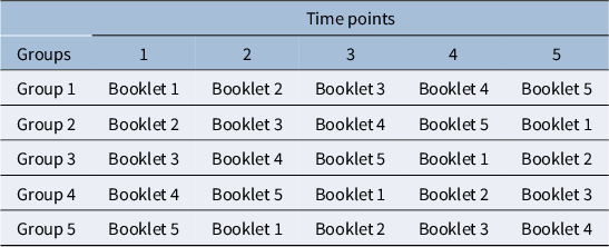
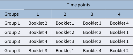

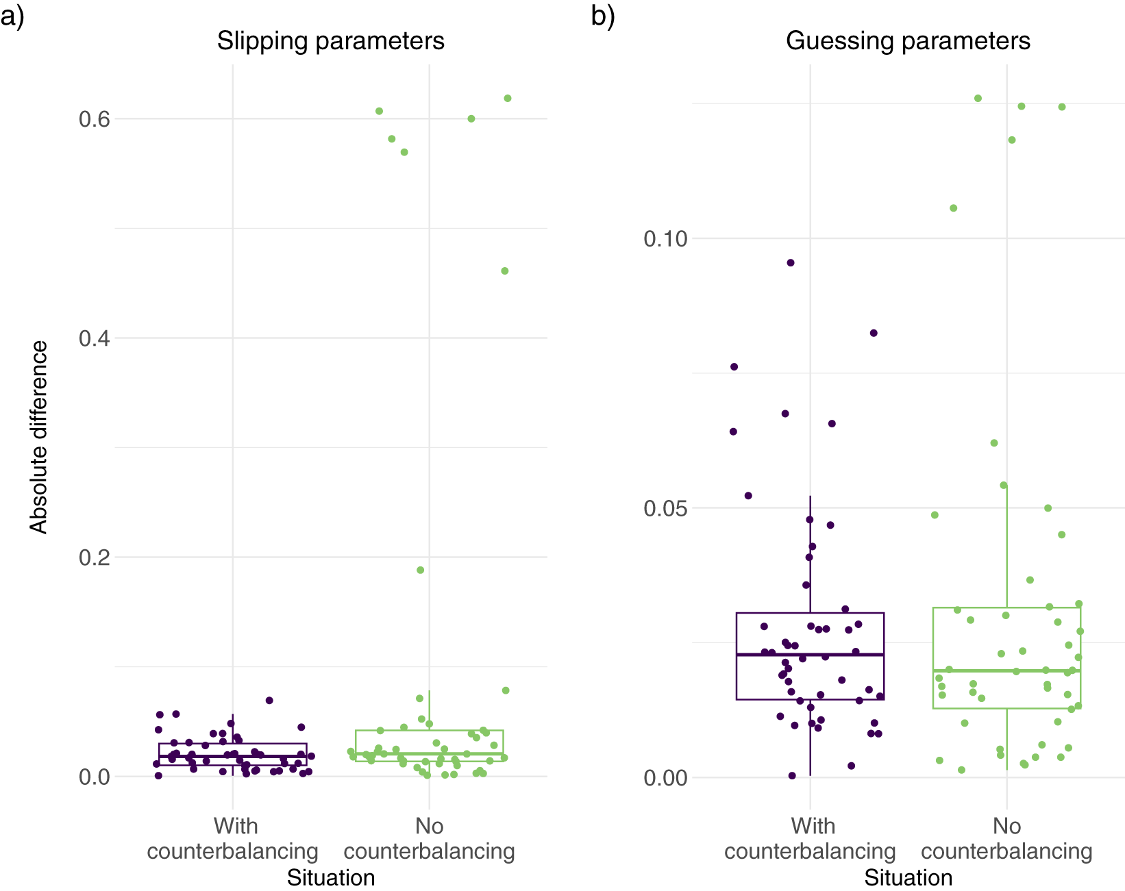
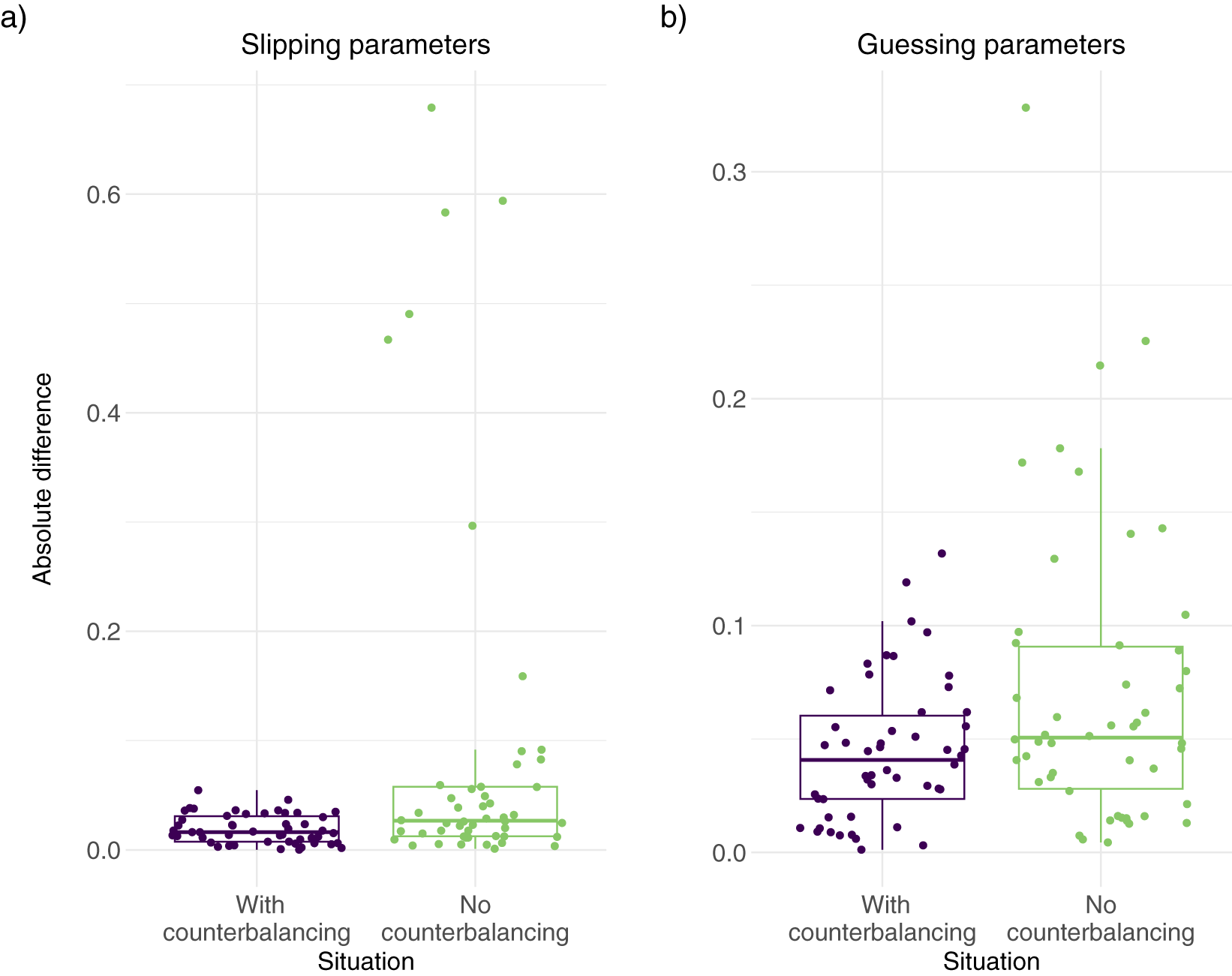
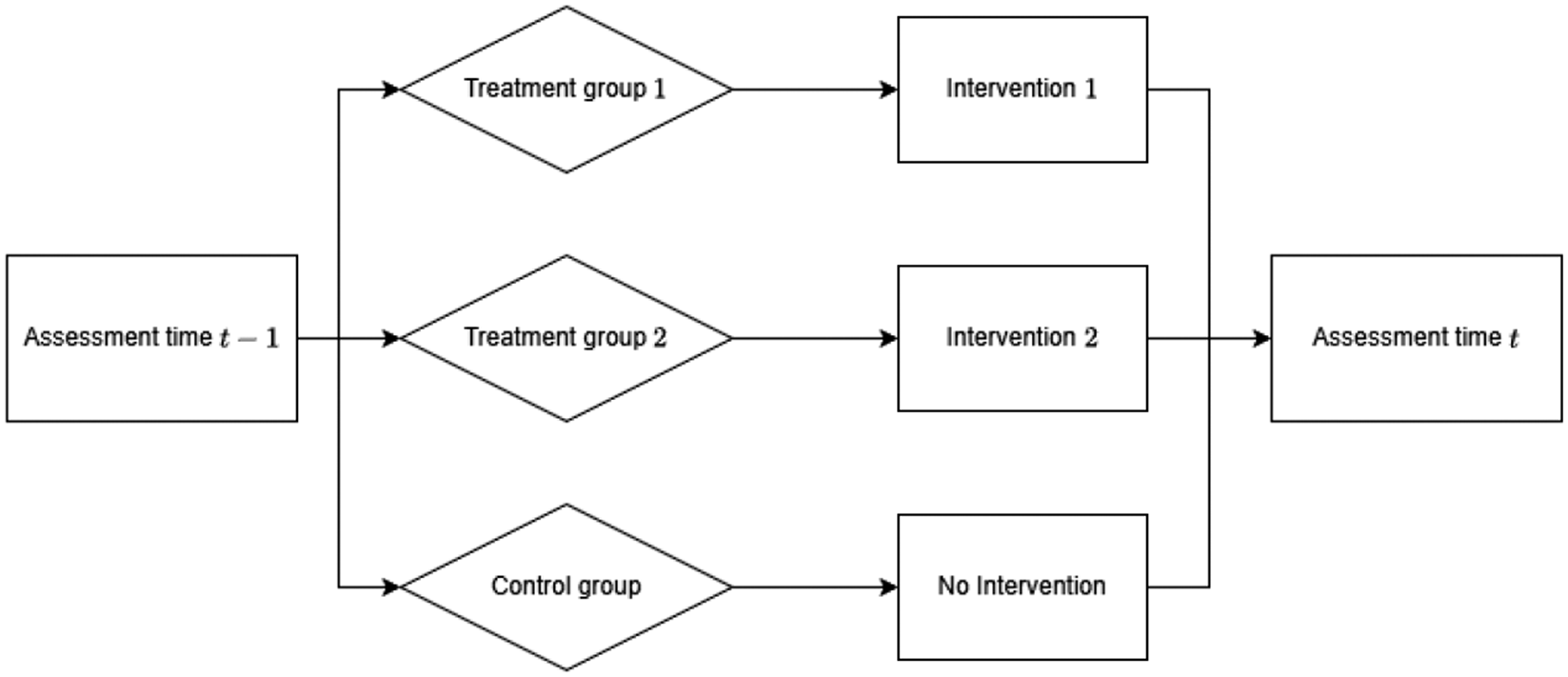
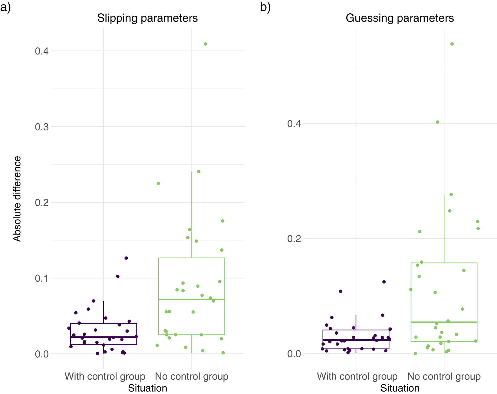
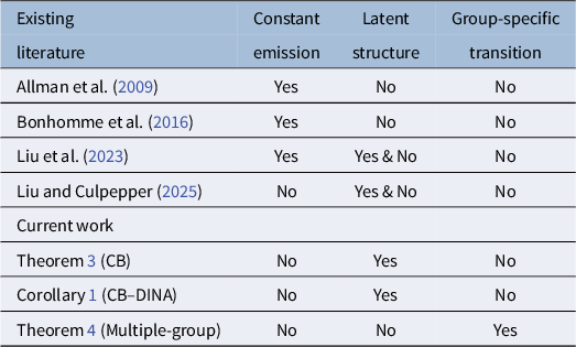
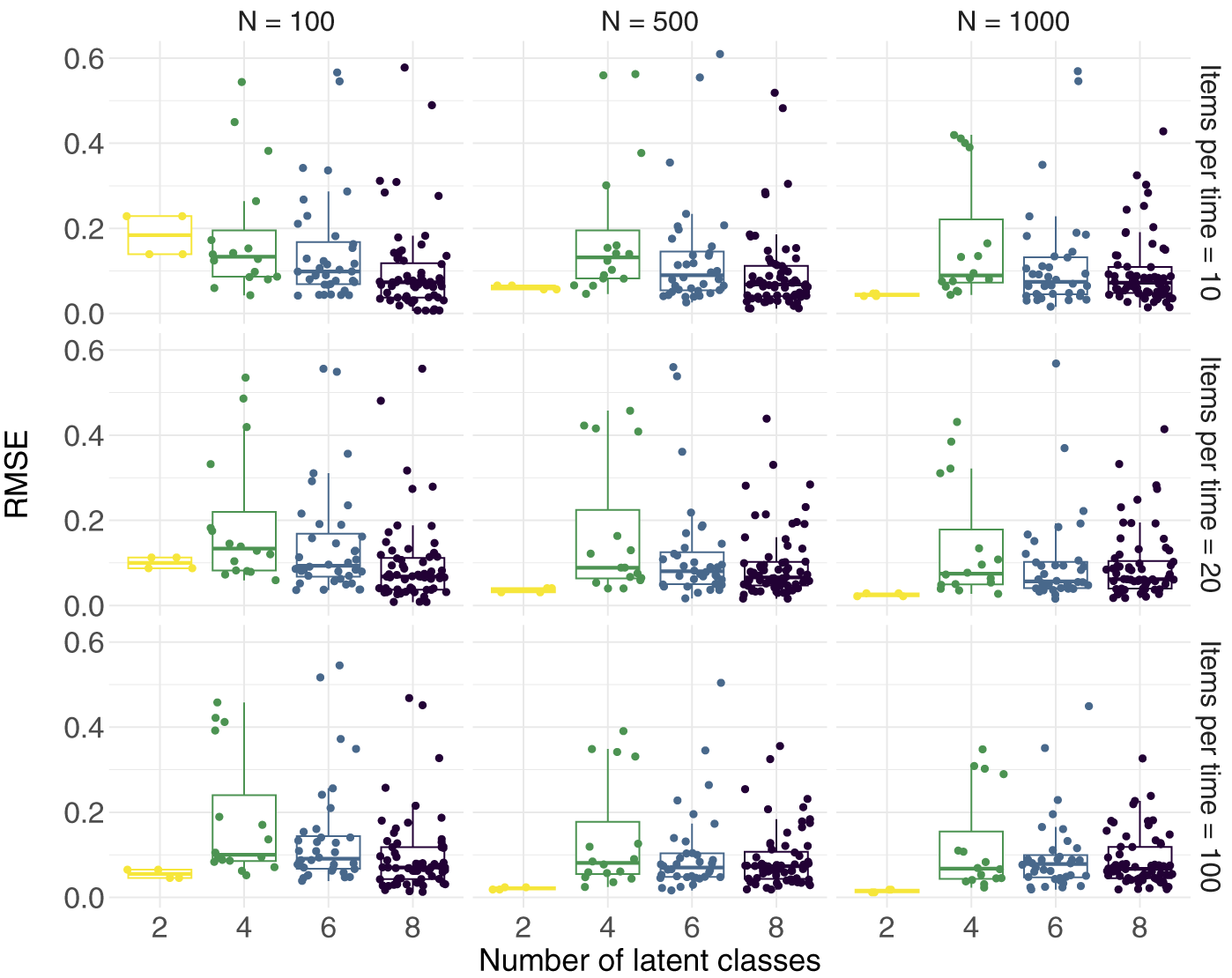
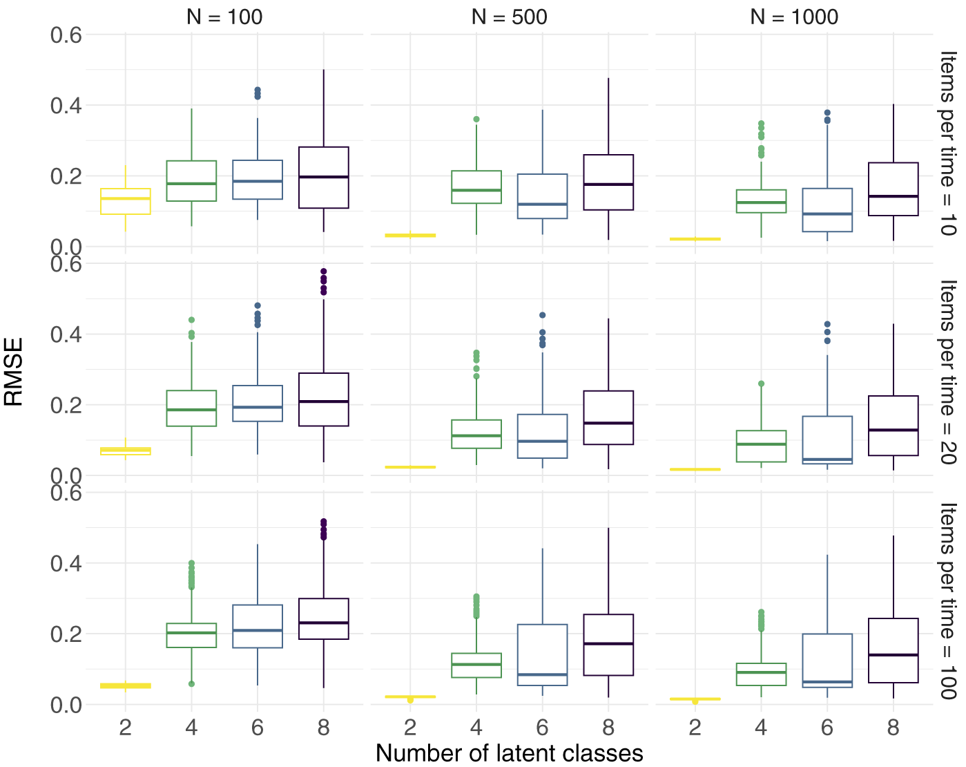
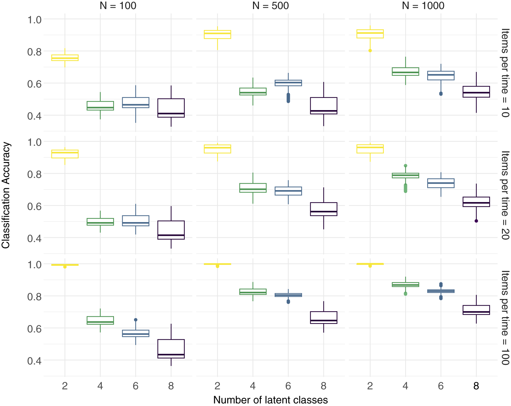
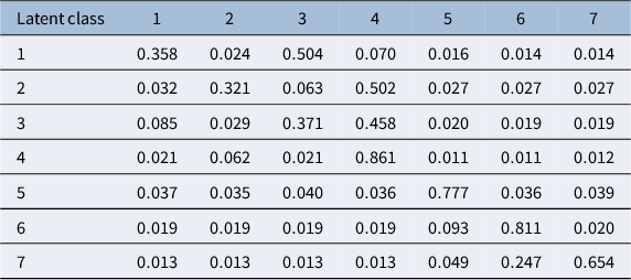
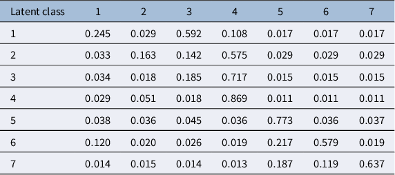
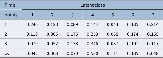
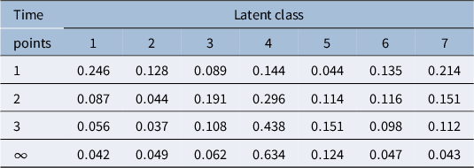
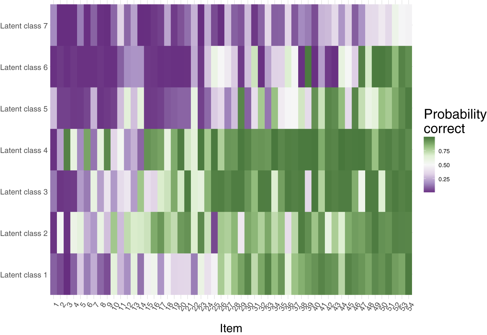

 Open access

