2 THE ORIGIN OF LITTLE h

In astronomy, everything in the Universe is moving relative to everything else. The Earth moves around the Sun, the Sun around the Milky Way, the Milky Way moves relative to the other Local Group galaxies, and the Local Group relative to more distant galaxies and galaxy clusters. Within the large-scale cosmic web we find bulk motions in every direction on the sky. Such relative velocity can be measured using a variety of techniques depending on the objects of interest. For galaxies, this is typically achieved through the identification of known spectral features that shift from where they should be because of their relative motion. The degree of this shift is known as either redshift (for galaxies moving away from us) or blueshift (for galaxies moving towards).

It was then a curious set of observations in the early 1900s that revealed that the majority of objects outside our own galaxy (then called nebulae, now known as other galaxies) were all moving away from us (i.e. redshifted), and in approximate proportion to their distance, called the distance–redshift relation. This was explicitly seen in the pioneering work of Slipher (Reference Slipher1917), Lundmark (Reference Lundmark1924), and Hubble (Reference Hubble1929), amongst others of the time. Although Hubble is often credited with its discovery, closer examination shows a more complex history with no one single eureka moment (see Peacock Reference Peacock2013). However, suffice to say that once the correlation was established, its ramifications changed our understanding of the Universe.

This relationship has since come to be known as Hubble's Law, written as

(1) \begin{equation} v = H_0\, d , \end{equation}

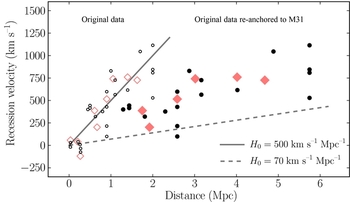
where v is the recession velocity of the galaxy, d is its proper distance, and the proportionality constant, H ₀ (Hubble's constant), was determined by fitting the data and has units of inverse time. Hubble estimated H ₀ ~500 km s⁻¹ Mpc⁻¹, as shown on the left-hand side of Figure 1 (open symbols and solid line), where we have reproduced the data and fit from his original paper (we will discuss the closed symbols on the right-hand side below).

Figure 1.

Hubble's original measurement of distant galaxies (Hubble Reference Hubble1929), plotting their redshift against distance. The left side shows Hubble's published data (open symbols): black circles mark individual galaxies, red diamonds group these galaxies into associations, while the solid line is his fit to the relation v = H ₀ d, where H ₀ = 500 km s⁻¹ Mpc⁻¹. However, the distances Hubble used are now know to be wrong. Following Peacock (Reference Peacock2013), we re-anchor Hubble's distance ladder to the correct value of M31 and replot the data on the right side (closed symbols). The dashed line shows Hubble's Law assuming H ₀ = 70 km s⁻¹ Mpc⁻¹, close to the modern value. Clearly there were greater problems with Hubble's original distances than just its local calibration.

The observed ‘fact’ that every distant galaxy in the Universe appears to be red and not blueshifted is itself remarkable. In effect, it tells us that the motions of all galaxies beyond our local volume are in a direction away from us, and the Hubble diagram shows that the further away a galaxy is, the faster its recession velocity. This was, of course, predicted by a simple solution to Einstein's equations of general relativity assuming a Friedman-Lemaître-Robinson-Walker metric, where the scale factor was shown to have a time dependence. A somewhat crazy idea when first discovered, Einstein himself was dissatisfied with the concept of a dynamic space–time, which led him to add his famous cosmological constant, Λ. However, that is a story for another time (in a slightly expanded Universe).

During the second half of the 1900s debate raged (primarily between de Vaucouleurs and Sandage) as to the precise value of H ₀, with observations placing it either close to 50 or 100 km s⁻¹ Mpc⁻¹ (see the excellent review by Tammann Reference Tammann1999, and references therein). The significant difference here with Hubble's original measurement was due to errors in the earlier distance calibrations (see below). The modern value of H ₀, measured to about 2% accuracy, is 67.3 ± 1.2 km s⁻¹ Mpc⁻¹ (Planck Collaboration et al. 2013). This means that a galaxy 1 Mpc away from us is receding with a velocity of 67.3 km s⁻¹ due to expanding space, a galaxy at 2 Mpc is receding at 134.6 km s⁻¹, and so on.

Returning to Figure 1, following Peacock (Reference Peacock2013) we create a modern version of this iconic plot by re-anchoring Hubble's distance ladder using the known distance to M31 of 0.79 Mpc, then re-scale the data appropriately. This is shown on the right-hand side with closed symbols. Also shown is a fiducial Hubble Law assuming 70 km s⁻¹ Mpc⁻¹ (dashed line). The lingering disagreement reveals Hubble's distance problems ran deeper than simply calibration uncertainties. As Peacock (Reference Peacock2013) argue, he was perhaps somewhat fortunate to be able to demonstrate any distance–redshift relation given the data he had on hand at the time.

Regardless, measurement (and later confirmation) of the Hubble expansion heralded in the age of modern cosmology. It underpins our modern cosmological paradigm. It factors into all observed galaxy properties that need to assume a cosmology to be measured. In short, it is important and must be understood.

3 LITTLE h DEFINED

Hubble's Law, as given by Equation 1, describes the relationship between the recession velocity and distance of a galaxy. For practical application Hubble's constant is often re-expressed as

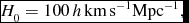(2) \begin{equation} H_0 = 100\, h\, \mathrm{km}\,\mathrm{s}^{-1} \mathrm{Mpc}^{-1} , \end{equation}

where h is the dimensionless Hubble parameter, pronounced ‘little h’.

The subscript ‘0’ in H ₀ indicates a measurement at the present epoch and sets the normalisation of Hubble's Law. However in general, the value of the Hubble ‘constant’ actually depends on redshift. Measured at redshift z by an observer at redshift zero,

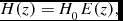(3) \begin{equation} H(z) = H_0\, E(z) , \end{equation}

where

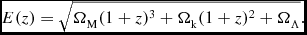(4) \begin{equation} E(z) = \sqrt{\Omega _\mathrm{M}(1+z)^3 + \Omega _\mathrm{k}(1+z)^2 + \Omega _\Lambda } . \end{equation}

H(z), often called the Hubble parameter, will change with time in different ways depending on the mass (Ω_M), curvature (Ω_k), and dark energy (Ω_Λ) densities of the Universe. However H ₀ does not change, and thus by construction, neither does little h. In other words, little h is just a number, a constant.Footnote ¹ Remember this and repeat it to everyone you meet.

Note that the units of H ₀ are inverse time. Hence, the inverse of the Hubble constant has come to be known as the Hubble time, t_H :

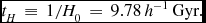(5) \begin{equation} t_H\, \equiv \, 1/H_0\, =\, 9.78\, h^{-1}\, \mathrm{Gyr} . \end{equation}

And the speed of light, c, times the Hubble time is just the Hubble distance, D_H :

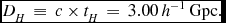(6) \begin{equation} D_H\, \equiv \, c \times t_H\, =\, 3.00\, h^{-1}\,\mathrm{Gpc} . \end{equation}

These are both fundamental numbers that astronomers often use as yardsticks against which to judge the relative age or distance of various cosmological properties. For further discussion on this and more we recommend the excellent paper, Hogg (Reference Hogg1999).

4 HOW LITTLE h ARISES IN THE MEASUREMENT OF GALAXIES

The Hubble constant is a global cosmological property of the Universe (at least in the vanilla ΛCDM paradigm) and not a local property of the individual objects within it (galaxies, gas, . . .). However, measurement of such objects does often depend on the background cosmology, and thus uncertainties about that background can propagate into the measurements themselves. In this way, the Hubble constant (typically expressed as the dimensionless little h parameter) can appear in the quoted values of galaxy (and other) properties. Significantly, from Equation 3, the fact that H ₀ is separable from E(z) is the reason why we can separate out little h in such measured quantities, even when the dynamics of the background cosmology are complicated and evolve.

Let us take a common but simple example from extragalactic astronomy. Observationally, the measurement of a galaxy's stellar mass often carries a h ⁻² dependence. So, picking a random example galaxy, its mass might be written as 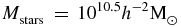$M_\mathrm{stars}\, =\, 10^{10.5} h^{-2} \text{M}_\odot$ . This particular h dependence arises from the way galaxy masses can be determined from the light that the telescope collects. In short, a galaxy's luminosity is drawn from the observed apparent magnitude and thus flux, the latter of which has units of area. Area has units of distance squared, for which each dimension carries the little h uncertainty through the angular diameter distance. Thus, galaxy luminosity carries an inverse h squared dependence. Moving from luminosity to stellar mass is non-trivial (one way is to multiply the luminosity by a stellar population model mass-to-light ratio). But throughout such calculations the h ⁻² dependence usually carries through.

In general, the key point to take away is that a galaxy property may or may not have a little h dependence, depending on how the property was measured. The measurement itself will determine how little h manifests in the property. Importantly, the numerical component of a property alone is not the value of the property. The value of the property is the combination of the number and the little h uncertainty (if one exists).

5 HOW LITTLE h IS PRESENTED IN THE LITERATURE

The above all sounds simple, right? If everyone presented their results in the same way it would be. But that's not what happens in the real world. Here we identify four broad cases outlining how astronomers have dealt with little h in the literature. Examples are given in Section 5.1.

• CASE 1: The authors do not mention the chosen H ₀ value in the paper, nor do they mention any of the h dependencies when the properties of galaxies are plotted or results given. Somehow we are magically meant to know what they assumed. Perhaps there was a standard practice back when the paper was written, but alas, that lore is long lost.

• CASE 2: The authors thankfully provide the chosen H ₀ value near the start of the paper (usually at the end of the introduction, or in the method section), and continue to assume this value throughout the paper. However, they omit all references to h when presenting their results and figures. To convert results between assumed Hubble parameter values you would either need to guess the h dependency (so hopefully it is a common and obvious one) or contact the authors for clarification.

• CASE 3: The authors mention the chosen H ₀ value near the start of the paper and then continue to assume this value throughout the paper, as per Case 2. However, unlike Case 2, when plotting figures and discussing results they continue to explicitly show all h dependencies with a subscript stating the chosen H ₀ value (e.g. h ⁻² ₇₀). This notation can potentially mean a number of things though, which we will illustrate below, so be warned.

• CASE 4: The authors do not choose a H ₀ value when presenting results and figures. Rather, properties that depend on little h have had it factored out and are labelled so that the dependence is clear. Such results are numerically equivalent to a cosmology where h = 1. Converting to your preferred H ₀ cosmology is as simple as replacing little h with the desired value and evaluating.

6 CONVERTING BETWEEN DIFFERENT HUBBLE PARAMETER VALUES

Let us say you understand all of the above, and have two sets of data that you would like to use in your paper. Perhaps one you have collected yourself and the other has been taken from the literature. Blindly comparing the numerical values in each data set will lead to problems if your data has assumed one of the little h cases listed in Section 5, and the literature another.

For example, if you are comparing the K-band magnitudes of galaxies, you may have to output your data assuming Case 4, i.e. with the h dependencies factored out. For the sake of argument, let us assume that the literature results you are comparing with have instead assumed h = 0.7, as per Cases 1–3. So although you may be able to find two galaxies (one from each data set) that appear to be numerically equivalent, they of course are not. Since little h typically manifests in galaxy absolute magnitudes as −5log ₁₀(h), any two such galaxies actually have a magnitude difference of 5log ₁₀(0.7) = −0.77.

So how would you go about re-normalising your galaxy magnitudes to the published h values? It is simple: since little h is just a number that has been factored out, replace all little h's with the h value you would like to assume and evaluate. This goes for any property where little h plays a part. Once the evaluation has been done, that property is then numerically correct for a universe where the Hubble constant equals that value.

Of course the same basic rules of mathematics apply when converting between different little h cosmologies, from h = 0.70 to h = 0.73 say. As long as you know how little h presents for each property of interest you can easily and systematically reverse then reapply any h value. This is one key reason why keeping the little h's visible can be particularly valuable. As a reference, in Table 1 we show how property values will change when moving from h = 1 (or h’less) to the commonly used value of h = 0.7.

Table 1

A simple chart for quickly converting a property with numerical value N from a h = 1 (or h’less) cosmology to h = 0.7, close to the currently favoured value and that used in Figure 2. Seven common little h scalings are shown. To go in the other direction, simply divide instead of multiply, or add instead of subtract.

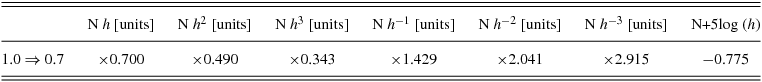
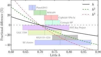
Figure 2 shows the fractional change in little h away from a value of 0.7, when h is rescaled to anywhere between h = 0.60 and h = 0.90, a range that brackets the currently favoured estimates (as indicated by the shaded regions). The three lines mark this difference for h, h ², and h ³ dependencies. With volume measurements (h ³) for example, there will be a shift of over 30% in a derived number between using the 2013 Planck H ₀ value (centred on h = 0.67) and that measured from SZ clusters (centred on h = 0.77). When properties are expressed with the h's factored out (Case 4 above), which is numerically equivalent to assuming h = 1.0, the discrepancy can be as large as 70% from Planck.

Figure 2.

To get a sense of the uncertainty in a property or result between two little h cosmologies, we show the fractional change in the property, relative to h = 0.7, when little h is changed continuously from 0.60 to 0.90 (this brackets the currently favoured range). The three lines show the change for little h dependencies of h, h ², and h ³, as marked in the legend. Different measurements of the Hubble constant from the literature are highlighted by the shaded regions (±1σ, and spaced arbitrarily along the y-axis for clarity), taken from figure 16 of the Planck 2013 XVI results paper (Planck Collaboration et al. 2013, and references therein).

7 COMPARING OBSERVATIONS WITH THEORY

If you are not using (or interested in understanding) theory-related data, then you can probably skip this section. For those who do (and are), the whole little h ambiguity rises to another level when you begin comparing models with observations (which is one of the primary uses of theory data, right?).

To start with, let us assume you have obtained a popular galaxy formation model so you can over-plot its predictions against some of your own results. When using someone else's data, the first step is to understand how it was generated and the units. In particular, where appropriate one must determine which of the above four cases (or other) apply to the assumed little h so that the correct conversions can be made to enable an apples-to-apples (a.k.a. fair theory-to-observation) comparison.

On the other hand, you may instead want to build your own model. Such models often must be calibrated, and this is where a reference set of observations are employed. Let us do this as an exercise, taking the standard practice of using the observed stellar mass function to calibrate the efficiency of the various model parameters. However beware! As mentioned in Section 5.1, mass in numerical data typically carries a h ⁻¹ dependence, in contrast to the h ⁻² dependence often found in observations (i.e. Section 4). The ‘one less power of h’ comes from the way mass arises in dark matter simulations.

To see this, consider an expanding universe where Hubble's Law reigns. As discussed previously, distance carries a h ⁻¹ dependence, and in fact, within the numerics of an N-body simulation, all distances typically have such a scaling. Now, the masses of simulated objects are usually calculated dynamically, expressed mathematically by

(7) \begin{equation} \frac{G\,m}{r}\approx \sigma ^{2} , \end{equation}

where G is the gravitational constant, and m is the mass contained within a radius r and supported against gravity by a velocity dispersion σ. Since r is simply a distance, when masses are determined—i.e. m∝σ² r—they pick up an inverse h dependence by construction.

The differing powers of h between simulation and observation must be accounted for before proceeding, and for those unclear about what little h actually represents this can be a dangerous trap. For example, which set of properties should be converted, the observations or the model, and how exactly? One may think that the model properties must all be made to have exactly the same factors of h as the observations, e.g. by multiplying all model masses by an additional h (see one of the real-world examples in Section 5.1). But this would be a grave mistake of course. On the other hand, a tempting compromise is often to explicitly factor out the h's (i.e. Case 4 above) delaying a determination of the full numerical values of each property, perhaps until one can say with greater precision what the Hubble constant actually is.

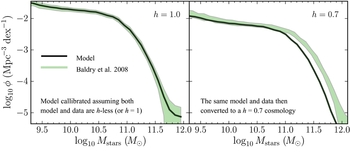
Let us do exactly this second suggestion and calibrate our model galaxy stellar mass function against its observational equivalent, in both cases keeping the (different) little h's factored out. We plot the result of such an exercise with the solid line in the left panel of Figure 3 and compare it to observational data marked by the shaded region (Baldry, Glazebrook, & Driver Reference Baldry, Glazebrook and Driver2008). Note the good match of the model is due to a precise calibration against the data. Note as well that this is typically how models have been historically calibrated and presented (see Croton et al. Reference Croton2006 and Bower et al. Reference Bower, Benson, Malbon, Helly, Frenk, Baugh, Cole and Lacey2006 for two popular and well-cited examples).

Figure 3.

We highlight one of the potential pitfalls when calibrating models against observations if you do not first assume a value for little h. In the left panel we show the stellar mass function of galaxies at z = 0, where all h's have been explicitly separated out (Case 4 of Section 5), numerically equivalent to a universe where h = 1.0 (and hence marked this way). Here the model (solid line) has been calibrated perfectly against the data (shaded region; Baldry et al. Reference Baldry, Glazebrook and Driver2008), as is commonly done. In the right panel, we then update both model and data for a universe where h = 0.7 (close to the actual value). Notice that the good agreement has been lost. This is due to the different ways in which the Hubble constant manifests in these different data sets, as discussed in Section 7.

Now let us assume that a new set of cosmological measurements are published locking the value of little h down to good-enough precision to be applied to our results. Remember that, as emphasised earlier, little h is not a unit; it is part of the numerical value of a measurement, just an uncertain part that we were able to factor out. Once we know what it is we probably should use it.

So what will taking this new little h value do to our well-tuned result? We can expect there to be a re-normalisation along the y-axis, as volume has a h ⁻³ dependence for both model and data. Along the x-axis, however, the model will be shifted by one power of h, while the data shifted by two. The right panel of Figure 3 shows this result for h = 0.7. Note the good calibration is now gone. So, for this particular galaxy formation model, was the original calibration good or bad?

The lesson is to know what little h is and how it manifests in both the observations and theory, before the data is used together. Our general advice for modellers and simulators is to always work with a H ₀ value as close to the best measured value at the time, while clearly stating the scalings for each property. In other words, do not factor out little h under the guise of convenience; this is not accurate and can lead to problems later on.

Finally, when it comes to the Hubble constant and simulations, it is important to remember that N-body and pure adiabatic hydrodynamic simulations are (generally) completely scale-free, in that little h can be factored out of all properties and the simulation scaled to any h value in post-processing. This of course also holds true for the semi-analytic and halo occupation distribution models that are constructed on top of N-body simulation merger trees. However, for more sophisticated hydrodynamic simulations, where absolute time-scales, distances, temperatures, etc. need to be established to model processes like cooling, star formation, and supernova feedback, such little h scaling breaks and one can only work with the Hubble constant assumed when the simulation was originally run.

8 SUMMARY: RECOMMENDATIONS FOR USING AND EXPRESSING LITTLE h

On the surface, the use of little h when quoting the values of observed or simulated galaxy properties appears simple. However, in practice it can get confusing due to the different ways the Hubble constant can manifest in data, and the different ways that authors present their results.

In this paper, we provide an introduction to the origin of the Hubble constant and the definition of little h, describe how little h arises in the measurement of galaxy properties (notably for survey data), and highlight four general ways in which little h is commonly expressed in the literature. We then walk through the method to convert between galaxy properties that have been expressed using different values of the Hubble constant. This is notably tricky when comparing observed and simulated results, where the same galaxy property can have a different little h dependence.

Our take-home message is this: First, the clearest way to express your results is to state the h scaling of each property at the beginning of your paper, then evaluate all properties assuming your best guess for the actual h cosmology of the Universe, e.g. h = 0.7. Once that is done for all results presented (measured in as many different ways as you like), each numerical value will be the actual value (assuming that cosmology) and can be compared with any other having the same units.

Second, the most sensible, less error prone approach to little h is to treat it like any other uncertainty in the data. The Hubble constant is a relic of bygone times. It is one of the least uncertain parameters in astrophysics, and the case for continuing to single it out as an independent parameter is weak.

Third, we emphasise that little h is not a unit. Units are physical quantities, like $\text{M}_\odot$ , Mpc, and km s⁻¹. It is best to be explicit about this. If you feel compelled to display little h when presenting each result, then separate out the units of the property from the combination of the numerical value and little h. For example, masses should be written 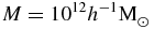$M = 10^{12} h^{-1} \text{M}_\odot$ , not 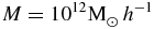$M = 10^{12} \text{M}_\odot \, h^{-1}$ or $10^{12} \text{M}_\odot /h$ . The latter two imply the h is coupled to $\text{M}_\odot$ , which is not true.

To conclude, in Table 2 we provide a list of common galaxy properties, their little h dependencies, and popular units to aid the uninitiated data user. Our key points are summarised below in a ‘cheat sheet’ providing nine rules for dealing with little h. Follow these and we will all live happier lives as a result.

1. 1 Little h is NOT a unit. h expresses an unknown part of the numerical value of a property. Units are $\text{L}_\odot$ , Mpc, etc. h is a number.

2. 2 Little h manifests in a galaxy property due to the method of measurement. For example, to measure the luminosity of a galaxy its luminosity distance must be known, and cosmological distances carry a h dependence.

3. 3 In general, when h is presented in a property you know that the h dependence has been factored out, with the h scaling explicitly shown.

4. 4 To put the property into a particular h cosmology, replace the h in the property with the desired h value and evaluate.

5. 5 To change from an already assumed h to a new value, reverse the above by doing the opposite with the assumed h. You can then substitute the new h value in.

6. 6 The terminology ‘h = 1.0’ and ‘h's factored out’ are often used interchangeably in the literature. Mathematically, the numerical value of a property will be identical. But in reality they represent different things. The first assumes a particular Hubble constant. The second assumes none and lets you decide at a later date.

7. 7 Sometimes the same property can be measured in different ways that have different dependencies on h, e.g. mass estimated from luminosity ( $h^{-2} \text{M}_\odot$ ), from dynamics ( $h^{-1} \text{M}_\odot$ ), or even in non-cosmological ways (e.g. reverberation mapping) that have no h dependence ( $\text{M}_\odot$ ). In such cases, as you change little h the different determinations of the property will scale differently.

8. 8 When you want to compare the same property that was obtained by two different ways having different dependencies on h (e.g. theoretical and observed masses), DO NOT transform one to match the h scaling of the other. Instead, choose a h value and convert both independently to that cosmology using point 4 above. Only then can they be meaningfully compared.

9. 9 Always clearly state what you have assumed with regards to little h at the start of your paper. For the love of God!

Table 2

An (incomplete) list of common galaxy properties, their little h scalings, and units.