

I. INTRODUCTION
When scientists realized the ability for computers to facilitate their work, they were perhaps the most enthusiastic early adopters of the technology. As computers became increasingly available in the 1950s, 1960s, and 1970s, scientists embraced them further and developed software to perform lengthy computations and to automate tedious data collection activities. Few fields were transformed as greatly as crystallography, through programs for direct-methods phasing and least-squares refinements and through computerized instruments. Fifty years later, the thought of recording measurements on a strip chart recorder seems as quaint as a commuting to work in a horse-drawn carriage.
There is now a plethora of highly specialized software programs for powder diffraction and practitioners also draw upon many general-purpose tools, such as spreadsheets and word processing packages. While use of computers and their power have grown in science, there is an irony that far fewer scientists are learning software development skills. This is a loss. While existing applications can accomplish quite a bit, there are always simple tasks in science that no one has programmed in a convenient way. Additionally, there are always new ideas that should be tried. Also of concern is the question of who will write the next generation of scientific software? Even when scientists team with computer specialists for software development, it is still very helpful when the scientists have a good understanding of the programming process. Hence, we recommend that more scientists learn to program. Fortunately, not only have computers become ubiquitous, but also the skills needed to learn programming have been simplified, at least with some high-level computer languages.
There are programming languages aplenty, with each computer language having been designed to fill a gap unmet in the capabilities of its predecessors, but even so, every language in common use has advantages and disadvantages, some of which will be considered below. Even professional programmers typically tend to specialize in the use of a small number of languages, but since scientists have considerably less time to invest, they typically prefer mastering a single language that can satisfy as many needs as possible.
Scientific computing requires that multiple types of tasks be done in combination: one needs to perform numerical or symbolic analysis, usually with a scientific software package to avoid reinventing the wheel; results need to be presented to the user, usually with scientific graphics; the user must interact with the program, typically in modern codes via a graphical user interface (GUI or web browser); documentation is needed to describe the software and for users to learn how to utilize the program. The Python programming language is able to perform all of this and more and thus satisfies what scientists need (van Rossum, Reference van Rossum1998). Furthermore, the authors of this paper feel that Python is among the easiest of languages for novices to learn, while being one of the best programming environments for scientific purposes, such as automation, image processing and numerical analysis. It also provides an environment where users can start with only the simpler capabilities, but possibly advance to using more powerful features, such as object-oriented programming, as skills grow.
Python offers capabilities for two different approaches to scientific computing: “numerical” vs. “symbolic” scientific systems. The former requires tools specifically meant to handle precise numerical data (e.g. Matlab, Octave, R-language, and other high-level computer languages), whereas the latter manipulates indefinite symbolic expressions or equations (e.g. Mathematica and Maple). Since all these features are available in Python, it can be applied to solve a wide range of problems. A novice can easily learn Python in order to turn their ideas into programs very quickly, but if needed for a larger project, she or he can learn to create object-oriented code, optimize code for speed and develop sophisticated scientific visualization with complex graphical user interfaces.
Furthermore, Python is a cross-platform open source software package that is licensed under the “Python Software Foundation License”, enabling the free distribution of the interpreter. Programs written in it incur no hidden licensing costs. This makes it ideal for use in the classroom, as well as in the laboratory, since replication of work is a cornerstone of the scientific method. Below, we will explain many of the features of Python and explain why it is so valuable for nearly all aspects of scientific computation, from quick-and-dirty format data conversion to model fitting through instrument automation and even first-principles theory. We first compare Python to some of the other programming languages commonly used in scientific computing, and then present a short overview of Python syntax.
What makes Python so valuable for scientific computation is not only Python's novice-friendly syntax, but also the many packages that allow many common programming tasks to be completed in dozens of lines of code rather than hundreds or thousands in other languages. Again, there are thousands of such packages, so we point out a small selection of these in order to highlight what makes Python so valuable and to point novices toward some of the most valuable resources. Finally, since a search for resources for learning Python can produce an overwhelming number of results, many of which are of limited value to a scientist, we provide a section (Appendix 2) with recommendations on many different types of pedagogical materials to help scientists learn to program with Python.
II. AN OVERVIEW OF MODERN PROGRAMMING LANGUAGES
Although there are many different programming languages, they fall into three general categories and it is important to understand the benefits and drawbacks of each approach. The original computer languages such as Fortran, Algol, Cobol, as well as more modern languages, such as C and C+ +, are interpreted by another large program called a compiler. The output of a compiler process is called machine code, because it contains the actual hardware instructions appropriate for the circuitry and operating system of a specific type of computer. A program compiled to run in Windows will not run on a Linux machine or on an Macintosh (except perhaps in an emulator) and, in some cases, a program compiled for a specific version of an operating system will not run on older or newer versions of the same operating system. After recompilation, code should be readily portable between computer platforms, but in practice this is not always true. The main advantage of using compilers is they produce the most powerful and efficient programs, since they take direct advantage of the computer and operating system design, but the cost is more of a learning investment and slower coding progress for the programmer.
Interpreted programming languages were developed as computers became more common and efficiency became less critical. In this, a master program called an interpreter reads the program to be run and as each line of code is encountered, it is translated and the requested actions are performed. One of the earliest interpreted languages was BASIC (circa 1964), but newer interpreted languages include Perl, Ruby, Tcl/Tk, and Python. These languages also tend to have sophisticated instructions that allow commonly used actions to be coded in a simple manner. This tends to both reduce the size of programs and simplify the process of writing them. Another advantage of interpreted languages is that a programmer can type individual instructions directly into the interpreter and experiment with the results. These two features allow programs to be developed with the minimum level of effort. Most interpreters are tested to perform identically on a wide range of computer platforms, which means that interpreted language program code will usually run identically on many types of computers. Initially these languages were used typically for writing simple and short programs, called scripts, so they are often referred to as scripting languages.
Interpreted programming languages do bring some disadvantages. One is that the interpreter must be installed on each computer where the program will be run. Furthermore, such interpreted programs tend not to run as efficiently as those in compiled languages. However, computational speed is often less of a concern than the time needed to create and debug a program. In the relatively rare cases where speed is a significant concern, usually only a small fraction of the lines in a program will impact this and many interpreted languages offer mechanisms for addressing these bottlenecks.
The newest type of computer language is something of a hybrid between compiled and interpreted languages. A compiler is used to convert the program to simple and generalized instructions called bytecode. Unlike the output from a compiler, these instructions are not specific to any type of computer hardware. To run the program, once converted to bytecode, a second program, called a virtual machine, reads these hardware-independent bytecode commands and performs the actual operations by translating them, command by command, to the actual hardware and operating system. Thus, bytecode will also run on any computer where the virtual machine has been ported. Java is the leading example of this type of language, which is available for a wide range of hardware, including all common personal computers and an estimated 109 mobile phones worldwide. It is even incorporated into most web browsers. The need for translation of bytecode to hardware instructions adds a layer of overhead, reducing performance to be typically intermediate between compiled and unoptimized interpreted languages. The code tends to be as complex and time-consuming to write as that of compiled languages, but has the advantage that the complied code tends to be quite portable, unless machine-specific packages are employed to improve speed, graphics, etc. Although these languages are quite attractive for professional programming tasks, a greater level of mastery is needed before they are useful for science and we cannot recommend them for casual use.
III. THE SYNTAX OF PYTHON
In later sections of this paper, we will provide some examples of Python code to explain different concepts. Readers who have no experience with programming languages or who wish to see how Python differs from other languages may want an introduction to Python syntax before continuing. This has been provided as Appendix 1. This also discusses the difference between the traditional (Python 2.7) and new (Python 3 or 3.x) versions.
As noted previously, the Python interpreter can be used interactively, so the programming commands below can be tried by typing them in a command window. In fact, many of the examples are shown as they would appear if typed directly into the interpreter, which uses prompts of >>> (or … for continuation lines). The same commands can also be placed in a file (sans the prompt characters), saved with the “.py” extension and the entire file can be run as a script.
In Section VII, below, an alternate approach for interactive use of Python, using the IPython shell is presented. When Python is used in that manner, input and output are prefaced with In [1] and Out [1] (where 1 will be subsequently incremented). Examples are also shown in that format, as well.
IV. MODULES AND PACKAGES IN PYTHON
What makes Python so valuable for science is the extensive library of modules that greatly extend a programmer's ability to perform different tasks. Note that if a package with the desired functionality is not already present, a programmer can create additional modules. Packages can be written in the Python language, or if speed or some other functionality is needed, in C, C+ +, or Fortran.
A. How to import packages
Python has some standard naming conventions for importing package modules within a program. Let's say our program requires that we import Pandas, NumPy and a section of the Matplotlib package. Normally this is done at the start of the program, as below:
In this case, we have defined abbreviations pd and plt to simplify later typing. To use the Pandas read_csv routine, we reference it as pd.read_csv. If only import pandas had been used, the reference would need to be referenced as pandas.read_csv. Python does allow us to eliminate use of these namespace prefixes by using the command from pandas import *, but this is a very poor programming practice. The prefix makes it clear to someone reading the code what routines are defined in the current module versus in another module or package. If from … import * is used with multiple packages and these packages contain routines with the same name, confusion is likely as to which routine will be accessed.
B. Built-in modules
There are more than 200 modules in the Python standard library, which are called “built-in” because they are distributed with Python as part of a basic installation. This “batteries included” approach provides the basic functionality that one would expect in any modern computer language. Examples of this include: the datetime module, which is used to interpret, compare, and manipulate representations of dates and times and the glob module which is used to search for files. Some of the modules provide more sophisticated functionality, such as sqlite3, a simple database implementation, and modules that allow Python to run a web server with very simple commands. There is on-line a complete list of built-in packages (https://docs.python.org/2/library/). One difficulty with Python is that because there are so many capabilities in the standard library, it can be difficult to locate the routine one needs – and there may be more than one way to complete an operation. Search engines such as Yahoo, Google, or Bing can also be useful. A query such as “Python find unique elements in list” will likely turn up a simple solution, such as that the call list[set(l)] will convert list l to a set, which only contains each unique element once and then converts the set back to a list, thus eliminating duplicates.
Scientists learning Python should certainly read the numerical processing modules (https://docs.python.org/2/library/numeric.html) section of the Python documentation. These modules provide capabilities such as trigonometric functions (but note that the NumPy package, Section V.A1, provides a faster alternative for these in array operations.) These built-in modules provide random number generation and also can be used to perform computations at arbitrary levels of precision, or even where rational numbers are stored and manipulated as exact fractions allowing certain types of computations to be performed with no round-off errors – infinite precision.
C. Add-on Python packages
As will be discussed below in subsequent sections, of great interest to scientists are the various “add-on” libraries and modules that are not formally part of Python, but add important features. These are written by individuals or groups of programmers and must be added to a basic Python installation. These modules are usually grouped into packages that have been written to solve particular needs or extend the capabilities of Python. For example, the Python packages for numerical processing will simplify coding and/or speed-up these computations. These additional packages, such as Python, are distributed as open-source and usually with non-restrictive licenses. These third-party add-on packages greatly expand the utility of Python, but introduce a complexity due to their separate distribution. A Python program that needs add-on packages requires a more complex Python “stack”, since both the interpreter and the package(s) must be installed wherever the Python program will be used.
It should be noted that while the transition from Python 2 to Python 3 discussed in Appendix 1 requires only minor changes in Python scripts (if any), but more extensive changes are needed for the code written in compiled languages that is used inside many Python packages. This has delayed availability of Python 3 versions of many scientific packages.
D. Python package managers and Linux distributions
Dependencies are an important problem in any computational environment and this gets complex for scientific Python, partly because the scientific stack evolved many years after the language was born. Hence, the packaging ecosystem for scientific Python is slightly messy and confusing for beginners of the language, because of various inter-dependent libraries and other dependencies. Python also has its own set of package managers exclusively built to handle this “dependency hell” for scientific Python distributions, with the most commonly used tools for package installation and dependency management:
-
• pip (https://pip.pypa.io/en/latest/) is the official Python package and dependency manager.
-
• conda (https://github.com/conda/conda/) a cross-platform binary package manager, an open source product of Continuum Analytics, Inc. (www.continuum.io), is particularly convenient.
The simplest solution is to find and install a single third-party distribution that provides Python configured with all the packages a user is likely to need. The most popular ones being:
-
• Anaconda (http://continuum.io/downloads) Note that this includes conda package manager.
-
• Canopy (https://www.enthought.com/products/canopy/).
-
• Python(x, y) (https://code.google.com/p/pythonxy/).
Anaconda and Canopy support Windows, Linux, and Macintosh computers, whereas Python(x,y) has distributions only for Windows and Linux.
Alternately, most Linux distributions have software installation programs and extensive libraries of well-tested software packages, which usually include many Python scientific software development resources. Among the most popular Linux versions, Debian, and Ubuntu use “dpkg” (https://wiki.debian.org/Teams/Dpkg) as the package management tool, while rpm-based systems such as Fedora/RedHat use “yum” (http://yum.baseurl.org) as their command line package management tool. GUI-based front-ends for running dpkg and yum are usually provided as well.
Other tools for Python version and environment management are:
-
• virtualenv (https://pypi.python.org/pypi/virtualenv) is a tool to configure Python so that only certain packages are visible. For example, this allows testing of software with selected versions of different Python packages when more than one version is installed.
-
• virtualenvwrapper (https://pypi.python.org/pypi/virtualenvwrapper) is a wrapper extension for virtualenv that makes its use more convenient.
-
• pyenv (https://github.com/yyuu/pyenv) Uses shell (e.g. Bash) scripts to manage installation of different Python versions.
V. A SURVEY OF ADD-ON PYTHON PACKAGES OF INTEREST TO SCIENTISTS
The PyPI site (https://pypi.python.org) provides an index to freely distributed Python packages. This site lists >40 000 packages (!), but not all are of equal quality and many are no longer maintained. Sometimes one can find historical evidence for parallel approaches to solving a problem before the community settles on a preferred method. Nonetheless, finding even an abandoned unmaintained set of code for a particular task can be of tremendous help in tackling a project. The large number of external packages is both a boon and something of an Achilles' heel for Python users. It is almost certain that one can find a package with routines of value for any project, but then it must be installed and if software will be distributed, users will need to do the same. This is why package management, as described previously, becomes so valuable.
Below we discuss some of the authors' favorite packages. All are available cross-platform on at least on all common computers, though perhaps not on smartphones and tablets. All are freely distributed. Not all of them are yet available for Python3.x, but this can be expected to change by 2015 or 2016 at the latest.
A. Computation
Dynamic typing makes Python easier to use than C. It is extremely flexible and forgiving, which leads to efficient use of development time. On those occasions when the optimization techniques available in C or Fortran are required, Python offers easy hooks into compiled libraries. Python ends up being an extremely efficient language for the overall task of doing science via software and is one of the reasons why Python use within many scientific communities has been continually growing. Below we discuss some of the packages that make mathematical computations easy in Python.
1. NumPy
NumPy is the foundational package used in scientific computing with Python. It is licensed under the BSD license, enabling reuse with few restrictions. Among other features, it supports operations on large, multi-dimensional arrays, and matrices that allow manipulation of N-dimensional array objects. It also provides a large library of high-level mathematical functions to operate on these arrays, including broadcasting functions on arrays. Other mathematical features include support for linear algebra, Fourier transformation, and random number capabilities.
The “ndarray” or the N-dimensional array data structure is the core functionality in NumPy, used as a container for many values (van der Walt et al., Reference van der Walt, Colbert and Varoquaux2011). However, unlike Python's “list” data structure, all elements in a single ndarray must have the same type; ndarrays can support multiple levels of addressing, which allows them to be used as multi-dimensional arrays.
To demonstrate the difference between a list and ndarray, let us consider that a Python list may contain a mixture of various data types:
In contrast, a NumPy array is typed. Here a nested list of integers is recast as a two-dimensional (2D) float array:
Note that above, all array elements are scaled (bitmap/255) in a single NumPy operation. With a list this would require a loop.
Since NumPy has built-in support for memory-mapped ndarrays, all NumPy arrays can be viewed into memory buffers that are allocated by C/C+ +. The requirement that all items in an NumPy array have the same type allows a more efficient memory access mechanism as compared to Python's object model and results in speedy calculations as compared basic Python. This ability to define efficient multi-dimensional containers of same-typed generic data across a variety of databases ensures data portability, a key requirement for large scientific projects. However, despite the modules that vectorize NumPy operations and call compiled code, NumPy may still be much slower than other modern languages like Julia and even optimized Fortran and C.
a. Performing efficient computations with NumPy
NumPy allows some computationally intensive computations to be performed with speeds comparable to that of Fortran or C codes (and sometimes exceeding them, since NumPy routines themselves are often highly optimized). Doing this requires writing the numerical calculations in a way that minimizes looping, where each NumPy function call will process as many values as possible, usually employing linear algebra and sometimes extending to arrays of 3, 4, or more dimensions.
As an example for how this works, let us compute a part of the structure factor equation:
 $${F_{hkl}}=\sum {{\,f_j}\exp \lsqb 2\pi i\lpar h{x_j}+k{y_j}+l{z_j}\rpar \rsqb }$$
To simplify this a bit, we can assume a center of symmetry, so that F hkl are all real and that f j is the same for every atom, and will be ignored. We then get:
 $${F_{hkl}}=\sum {\cos \lsqb 2\pi \lpar h{x_j}+k{y_j}+l{z_j}\rpar \rsqb }$$
We will define in Python the reflections as a nested list of hkl values, [[h 1 k 1 l 1], [h 2 k 2 l 2],…] such as
so ref[j] is [h j ,k j ,l j ] and ref [j][i] is h j , k j , or l j , for i = 0, 1, or 2, respectively. Likewise, we can define a nested list for atom coordinates, where atom[j] is [x j , y j , z j ] and atom [j][i] is x j , y j , or z j for i = 0,1, or 2, respectively:
The simplistic way to compute a list of F hkl values would then be to directly translate the mathematical formula for F hkl to Python, as one might write C or Fortran code with a doubly nested loop:
This works, but to show how this same computation can be done without any loops using NumPy, we can repeat this as a matrix computation. Note that we can cast the nested lists, atom and ref, into rectangular (2D) NumPy arrays. Note the shape member gives us the dimensions, (4 × 3) and (7 × 3):
The contents of the innermost loop, above, above computes an interior product, where each row of the two arrays are multiplied and then are summed. This can be performed with np.inner(), which yields a (7,4) array in a single call:
Note that np.inner() expects two ndarrays as input, but will cast our nested lists for us into that form. [We could avoid that by explicitly performing the conversion using np.inner(np.array(ref),np.array(atom)).]
This inner product multiples the first set of coordinates, [0.,0.5,0.5], by the first reflection, [1,0,0], element by element and then adds the three products to yield the first value in the first row (0). Then the second atom coordinates, [0.,0.5,0.5], are multiplied by the same hkl value, (yielding 0.5) for the second term in the first row (and so on). We can then easily multiply every element in the matrix from np.inner() times 2 and π and take the cosine of each term:
Note that the standard math module cos() function can only compute one value at a time, whereas the corresponding function in NumPy can handle single values as well as arrays. In fact, np.cos() can fully replace math.cos().
Finally, we want to sum the contents of each row, which can be done with np.sum(, axis = 1), where 1 refers to the second array dimension (since Python uses 0-based indexing, we count starting at zero).
Using this approach, we can reduce the previous example to five lines of code, but where all the computations are performed in a single line:
With the small number of values used above, this computation takes a negligible amount of time, but with more atoms and reflections, this is not true. This was demonstrated by repeating the above with 500 atoms and 5000 reflections. Then the computation using the first coding approach required 37 s to complete, while the second, with the single optimized line of NumPy code, required only 0.1 s.
2. SciPy
SciPy (http://www.scipy.org/scipylib/) is a package built on top of and distributed together with NumPy. It contains a wide variety of numerical analysis routines, such as real and complex Fourier transforms, integration, interpolation, image processing, and optimizers. It is used widely in fields ranging from electrical engineering through bioinformatics and oceanography and even finance.
SciPy has some nifty advanced features like “sparse matrices” – an almost empty matrix storing only non-zero items. Storing zeros is a waste of resources and computations can be simplified by only treating the non-zero elements. SciPy also has routines for: image manipulation, image filtering, object properties (segmentation), and feature extraction (edge detection).
3. Numba
Numba (http://numba.pydata.org) is an open-source optimizing compiler for Python, sponsored by Continuum Analytics, Inc. It adds just-in-time compilation to Python, meaning that when a designated computation is first needed, the compiler generates machine code optimized specifically for the computer being used at present. It integrates with NumPy and provides a possibility for computationally demanding sections of a program to be sent to specialized hardware (such as a GPU). It thus integrates with the older Python scientific software stack ensuring code portability, and often provides performance comparable to or exceeding traditional C, C+ +, and Fortran coding.
Numba uses two special codes called decorators, “@jit” and “@autojit” to speed up compilation and optimize performance. The jit decorator returns a compiled version of the function using the input types and the output types of the function. The autojit decorator does not need type specification. It watches the types called by the function and infers the type of the return. When previously compiled code exists, it is reused. If not, it generates machine code for the function and then executes that code.
4. Scikit-learn
Scikit-learn (http://scikit-learn.org) is a machine-learning package written in Python. Machine learning is a form of artificial intelligence for pattern recognition, where the software generates rules to classify information by being “trained” on input datasets that have already been classified. For example, k-means clustering is a popular algorithm for data mining from text documents. Another example of the clustering technique in machine learning is “unsupervised learning”, which tries to create structure within unlabeled data, where no pre-defined datasets are used. Scikit-learn was developed as an extension to SciPy.
5. Sympy
SymPy (http://sympy.org/en/) is a module for performing symbolic mathematics. Most scientific computation is performed numerically, e.g. where equations are evaluated with specific values. With symbolic processing, such as is implemented in Mathematica and Maple, the equations themselves are manipulated. Thus, SymPy can determine that the derivative of sin(x) with respect to x is cos(x). This is done directly on the expression and without use of any numerical values for x.
6. Theano
Theano (http://deeplearning.net/software/theano/) is another Python library for efficiently computing mathematical expressions involving multi-dimensional arrays. Most importantly, it has tight integration with NumPy, with dynamic C code generation support that allows faster expression evaluation. It supports symbolic differentiation and offers optimization and extensive unit testing.
Theano uses graph structures for defining all mathematical relations by using symbolic placeholders known as “Variables”, which are the main data structure-building blocks. Theano has strict typing constraints to allow it to tailor C code to statically optimize the computation graph. Variables can be an instance of a NumPy ndarray, or an array of 32-bit integers (“int32”) or have a shape of 1 × N. Broadcasting is a feature that exists in NumPy, but primarily for scalars and arrays. Theano extends broadcasting to cases where dimensions are added to an array. Another feature of Theano is the different types of computational optimizations that can be performed globally or locally.
B. Big Data Processing Packages
The term “Big Data” is used for computation involving very large collections of information, usually too large to fit in the memory of a single computer. For example in diffraction, experiments involving large numbers of area detector images can reach the scale of a terabyte.
1. Pandas
Pandas (http://pandas.pydata.org) is a powerful data analysis manipulation library for Python, which provides an easy tool for working with multi-dimensional data structures (McKinney, 2012). The documentation is available online (http://pandas.pydata.org/pandas-docs/stable/).
Matrix operations are commonly used in scientific computations and Pandas uses the “DataFrame” data structure, which makes it easy to work with data stored in relational databases, text or spreadsheet data files such as Excel files (tab- or comma-separated values), time-series financial data analysis, multi-dimensional arrays, and statistical regressions on large datasets. A DataFrame is essentially a “2D array” with rows and columns of data, such as a spreadsheet.
Creating a DataFrame from an original set of records is simple, and as an example, we use some financial data for General Electric (GE) stock that has been uploaded to a git repository (https://gitlab.com/aleph-omega/stockex-usa) for easy reference. (Note that these files are quite large in size.)
To show how adept Pandas is at accessing “spreadsheet” data, below we read data from the file into a DataFrame object using pandas.read_table for tabulation in the second line. The subsequent line slices through the DataFrame to pull in the first 11 records.
Furthermore, Pandas is excellent at memory management, which is crucial for handling Big Data. The “groupby” feature is especially helpful and can reduce lengths of Python scripts by an order of magnitude over what is required with other languages. We can achieve this by splitting our data into smaller groups, based on pre-defined criteria, and then by writing functions that will be applied to each group separately with the output being combined into a dataframe.
Pandas speeds up computation, as well as allows for rapid coding and improved code maintenance, since it is much easier to express a mode of analysis with fewer lines of code. Since operations such as merges, sorts, groupings, and creating new variables are performed within the package, in compiled and optimized machine code, the speed gain can be tremendous.
2. Blaze
Blaze (http://blaze.pydata.org) is a mechanism to build more complex data structures into the framework of NumPy and building on Pandas. Although the ndarray in NumPy requires arrays to have fixed lengths along each dimension, Blaze allows for much more complex structures. It also uses just-in-time compilation, as employed in Numba, to speed computations. Blaze is a fairly recent project, also sponsored by Continuum Analytics, Inc.
C. Statistics
Statistical capabilities are available in some of the previously discussed packages, but the packages described here are specifically designed for statistical analysis.
1. PyMC
PyMC (http://pymc-devs.github.com/pymc/) is a Python module for Bayesian statistical modeling and model fitting that focuses on advanced Markov chain Monte Carlo fitting algorithms, fitting sampling algorithms (such as Hamiltonian Monte Carlo), numerical optimization, and also for solving unconstrained non-linear optimization problems. Its flexibility and extensibility make it applicable to a large suite of problems.
2. Statsmodels
Statsmodels (https://github.com/statsmodels/statsmodels) is a Python library package for econometrics, plotting functions, statistical modeling, and tests, which provides a complement to SciPy for statistical computations, including descriptive statistics, and estimation and inference for statistical models. Researchers can explore data, estimate statistical models, perform statistical tests, and use it for their statistical computing and data analysis in Python. Statsmodels runs on Python 2.5 through 3.2 versions and some useful features it supports are:
-
• Linear regression models
-
• Generalized linear models
-
• Discrete choice models
-
• Robust linear models
-
• Many models and functions for time series analysis
-
• Non-parametric estimators
-
• A collection of datasets for examples
-
• A wide range of statistical tests
-
• Input–output tools for producing tables in a number of formats (text, LaTeX, HTML) and for reading files into NumPy and Pandas
-
• Plotting functions
-
• Extensive unit tests to ensure correctness of results
-
• Many more models and extensions in development.
D. Visualization and image-processing packages in Python
Python excels at the graphical display of data, which is an important aspect of scientific analysis. Graphical display can be separated into two categories: 2D representations and pseudo-three-dimensional (3D) ones. In the case of 3D, objects are portrayed as viewed from a particular direction, but that direction can usually be manipulated interactively. This allows the viewer's brain to interpret the representation as if an actual physical object had been seen.
A related computational task is the interpretation and transform of digital images. Some capabilities for image processing can be found in SciPy (5.1.2), but more sophisticated capabilities are also discussed below.
1. Matplotlib
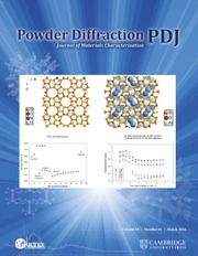
Matplotlib (http://matplotlib.org/) is a scientific 2D graphics library consisting of a programming interface that creates vector graphics representation and renders it for output display (Hunter, Reference Hunter2007). The advantage of vector graphics is that the resulting plots can be shown at very high quality, as might be used for a journal article or presentation. Matplotlib can also be used interactively to plot results, such as one might use in a spreadsheet environment. Simple Matplotlib commands can be used to generate graphics easily. As an example of how simple it is to use Matplotlib, in the following code example, NumPy is used to compute an array of 500 points over the range from 0.0 to 6π and then a new array is created containing the sine of each value in the previous array. Finally, the a plot is generated, where the x-axis is the first plot, but indicated in units of π and the y-axis shows the sine values:
The resulting plot, as it appears on the screen, is shown in Figure 1. Note that even with this very simple plotting command, the resulting plot is quite fully featured. The icons at the upper left allow the plot to be repositioned in the window, including “zooming”, and the plot can be saved as a higher resolution bitmap file. At the bottom, the position of the cursor is displayed as it is moved around in the window.
(Color online) An example of simple screen graphics from the Matplotlib package, generated with a simple command. Note that the plot can be shifted and zoomed. Also, the cursor position is indicated.
The Matplotlib package is also very well suited for creation of sophisticated graphics and readers are recommended to look at the web gallery (http://matplotlib.org/gallery.html) of very complex and beautifully formatted sample Matplotlib graphs and the corresponding (usually quite simple) example code to see what can be done with Matplotlib.
It is also possible to use Matplotlib for interactive applications, where the user can interact with the graphics through mouse clicks and the keyboard. This, however, is not always implemented as conveniently as might be liked.
2. Chaco
Chaco (http://code.enthought.com/projects/chaco/) is another scientific graphics library intended more for display than creation of “hard-copy” plots – it generates attractive static 2D plots. Although it also works well for interactive data visualization and exploration, it does not offer all the sophistication of Matplotlib, but it is quite easy to use.
3. Bokeh
Bokeh (http://bokeh.pydata.org) is an interactive visualization library for Python and other languages for making powerful graphical presentations. With graphics that rival the widely used D3.js JavaScript library, it delivers good performance with large datasets, but is integrated with Python. It works well with the IPython Notebook. Bokeh is compatible with Matplotlib. With it, programmers can easily create applications to deliver high-performance interactive visualization of large datasets.
4. Mayavi
Mayavi (http://code.enthought.com/projects/mayavi/) is a toolkit for 3D visualization of scientific data in Python, a part of the Enthought Tool Suite (ETS). Data plotted in Mayavi correspond to 3D objects that can be “rotated” on the computer display, allowing people to better understand the 3D nature of the displayed information. Mayavi is built on top of the very sophisticated VTK (http://www.vtk.org/) system, which also provides a Python interface. The interactive 3D display graphics are performed using a combined hardware/software protocol known as OpenGL. Alternately, very high-performance interactive graphics can be performed in Python with direct use of OpenGL calls through use of the PyOpenGL (http://pyopengl.sourceforge.net/) package, but this is considerably more difficult and is not recommended for most uses.
5. Scikit-image
Scikit-image (http://scikit-image.org) is a machine-learning module built on top of SciPy specifically for image processing (see scikit-learn, above), Source code (https://github.com/scikit-learn/scikit-learn).
6. PIL/pillow
PIL (http://www.pythonware.com/products/pil) is the Python Imaging Library. This contains routines for reading and processing images. This library is a simple and useful tool for those starting out with image manipulation to learn the basics. However, it had not been updated in some years and support for Python 3.x was not planned. Hence, a fork-called pillow (https://pypi.python.org/pypi/Pillow/) was developed to enhance PIL. The two projects were later integrated into a single codebase, so that the packages are largely interchangeable.
As an example of how this package is used, we will read a rather famous image file from Wikipedia and perform some simple processing steps.
These commands read and display the image and then convert it to black-and-white.
We can examine the image file. In the output below, the format attribute tells us that this is a JPEG image while the size gives us the image width and height in pixels. Finally, the mode attribute supplies pixel type and depth.
PIL allows images to be converted between different pixel representations, so we will use the convert() method to convert the above-mode attribute (RGB) to luminance (“L”). The output from this is shown as Figure 2. Here each pixel is colored by the luminance value using an arbitrary color scale to show the values (this scale can easily be changed).
Not only can the Python Imaging Library (PIL) be used to perform image manipulations, but images can also be exported as ndarrays, so that Numpy and Scipy computations may be performed on them.
(Color online) An image that has been recolored to show the luminance of each pixel according to a Matplotlib color mapping.

E. Python for instrument automation
The ubiquity of computers in science extends to instrumentation; many scientific instruments are computer-automated to reduce operational complexity. Other instruments have sophisticated automation to the point of allowing remote or even unattended operation. Python is an excellent choice for automating instruments, since it can support libraries that will perform the low-level communication with instrument hardware and also higher-level computation and graphics. Likewise, it is also relatively easy to create high-quality graphical user interfaces or web applications for eventual user control. For Python to control a scientific instrument, a device driver that implements the communication protocol(s) to the instrument electronics is needed. For common communication protocols, such as RS-232 devices (http://pyserial.sourceforge.net/) or EPICS (http://cars9.uchicago.edu/software/python/pyepics3/) there exist standard communication libraries. If a vendor provides a function library, such as a Windows “.DLL” module or Linux “.so” library, the ctypes module in the Python standard library can be used to access those functions.
The fact that Python code can be executed interactively greatly simplifies creation of an applications programming interface. For example, the highest resolution and most productive powder diffractometer in the USA, the 11-BM instrument at the Argonne Advanced Photon Source, is automated completely in Python (Toby et al., 2009). A video (http://youtu.be/86TZpk_Tn1M) is online. The library that drives the appropriate motors, coordinates use of the robot and ancillary equipment, such as for sample temperature control, was initially developed by typing commands into the Python interpreter and then collecting the code that worked. The result was a library of ~3000 lines of code and comments, which provides routines to initialize and drive the instrument, to load or unload a sample or read a sample's barcode, set a temperature, perform a data collection scan, etc. From that point, it was relatively straightforward and only another 1000 lines of commented Python to develop routines that query the instrument database for the details of data collection for each sample, optimize the data collection sequence, and then perform the actual scans. Finally, ~1000 more lines of code were used to develop a graphical user interface that allows an operator to fine-tune data collection parameters. The resulting software can run the instrument for days at a time unattended; recover from loss of the synchrotron beam; and even send text messages to alert an operator, if the program aborts because of unexpected problems.
VI. GRAPHICAL USER INTERFACES
Increasingly, scientists wish to create programs with graphic user interfaces (GUI) – applications that display in windows and have buttons and menus that are used to control the program execution. Python has an integrated GUI package, Tkinter, in its standard library, but use of this is not recommended, since it is a grafted version of the Tcl/Tk language that is rather clumsy to use in Python. In addition, the resulting GUIs have a rather antique appearance.
Two very widely used cross-platform C ++ packages, wxWidgets (http://www.wxwidgets.org/) and Qt (http://qt-project.org/) (pronounced “cute”) have Python libraries that are widely used. Qt was developed and released for open access by cellphone manufacturer Nokia, is newer, and seems to be attracting more attention at present. The alternative, Python package wxWidgets has been in use for quite a while and has a large user base. Each will be discussed below.
It should be noted that regardless of which package is selected, GUI programming requires a change in programming paradigm. Traditional software is usually written in a linear fashion, where the program starts, reads some input, produces some results, and stops. GUI-based programs are event-driven, which means they perform a series of initializations when starting and then go into hibernation (in an event loop) and from that point only respond to user actions such as mouse clicks, which in turn initiate “callback” routines. Most code is placed in routines that will be triggered only through these callback routines. A GUI program will typically stop only when a callback routine ends the program.
An alternate approach to creating a GUI for software is to provide access to it from a web browser. This is typically not a method of choice for very sophisticated interfaces, but is surprisingly effective for many scientific computations. Python has a number of mature web application frameworks, such as Django (https://www.djangoproject.com/), available for building web sites. As one example the capability of Python for web applications, very large portions of the code used to run the YouTube web site are written in Python. Other languages such as PHP, Java, Ruby, and JavaScript are also used for creating web applications, but these languages do not have the wealth of scientific packages that Python has, so scientific projects using those languages frequently require components to be written in another language. While this is frequently done for commercial work when large teams manage different aspects of a project, using Python for the entire application stack greatly simplifies both development and maintenance tasks, facilitating smaller-scale scientific projects.
Another alternative for GUI programming is through the IPython Notebook architecture, which allows notebooks to have interactive widgets (http://nbviewer.ipython.org/github/ipython/ipython/blob/2.x/examples/Interactive%20Widgets/Index.ipynb). Notebooks can provide the benefits of command line interfaces and graphical interfaces. The IPython package will be discussed in Section VII.
1. PyQt and PySide
PyQt (http://www.riverbankcomputing.com/software/pyqt/intro) is a Python binding of the cross-platform GUI toolkit Qt, providing GUI programming in Python. PyQt is free software implemented as a Python plug-in, but because of license restrictions is avoided by some commercial organizations.
PySide (http://qt-project.org/wiki/pyside) is an alternate and more recent open-source Python binding for Qt, which was fostered by Nokia and avoids the licensing problems that arose with PyQt. PySide is not completely mature software, but it is widely used and should be highly reliable soon, if it is not at that point already. The authors have no experience in use of PySide at present, but would likely select it over wxPython if they start a new project requiring a complex GUI.
2. wxPython
wxPython (http://www.wxpython.org/) is a Python binding package for wxWidgets (Rappin and Dunn, Reference Rappin and Dunn2006). It is a very comprehensive package offering a great wealth of GUI tools that can be adapted into a project. One of this article's authors (BHT) has considerable experience with writing wxWidgets-based GUI codes, for example with the GSAS-II Rietveld code (Toby and Von Dreele, Reference Toby, Huang, Dohan, Carroll, Jiao, Ribaud, Doebbler, Suchomel, Wang, Preissner, Kline and Mooney2013; idem, Reference Toby and Von Dreele2014), but still does not find all aspects of this coding to be straightforward.
In order to make wxPython compatible with Python 3.x, the package was redeveloped and initially released in a new version in 2013 called “phoenix,” while the original version is called “classic.” At present both are being updated in parallel. It is unclear how much effort will be needed to migrate programs between the two.
VII. PYTHON APPLICATIONS
There are many applications that are based on Python or offer programming capabilities in Python. As one example, Sage (http://www.sagemath.org) is a freestanding mathematical software package with features covering many aspects of mathematics, including algebra, combinatorics, numerical mathematics, number theory, and calculus. It uses many open-source computation packages with a goal of “creating a viable free open source alternative to Magma, Maple, Mathematica, and Matlab.” It is not an importable Python package, but does offer a convenient Python programming interface. Sage can also be used for cloud-based computing, where a task is distributed to multiple computers at remote sites. Other examples include: Spyder (https://pythonhosted.org/spyder/) a code development and computing environment and Enthought's PyXLL (https://www.pyxll.com/), which allows Python to be embedded into Excel spreadsheets.
The IPython program is one of the nicest tools to emerge out of the Python community (Pérez and Granger, Reference Pérez and Granger2007). The IPython output (notebook file) architecture is built on top of widely used protocols such as JSON, ZeroMQ, and WebSockets, with CSS for HTML styling and presentation and with open standards (HTML, Markdown, PNG, and JPEG) to store the contents. The IPython program is now starting to be used as a programming environment for other languages, since much of the capabilities are general and because of the use of open standards, other programs can read the notebook files.
The IPython notebook serves many purposes including: code prototyping, collaboration, reviewing documentation, and debugging. It incorporates tools for profiling code, so that if a program is too slow, the (usually short) sections of the code that are taking the most execution time can be quickly identified and reworked. It integrates well with matplotlib and NumPy and can be used as one might employ Matlab, to interactively analyze data, with integrated graphics and computation. Finally, IPython provides a mechanism for remote execution of Python commands. This can be used to distribute a large computation to a supercomputer. Since Python commands and intrinsic data objects are portable, the remote computer can be a completely different architecture from the controller. Perhaps the biggest problem with IPython is how to master all the features.
A. IPython as a shell
Many developers utilize IPython as an interactive shell to run Python commands and rarely invoke Python directly via a command window. It provides many advantages over running Python directly, chiefly, code completion: if a part of a command or function is typed and the tab key is pressed, then all of the possible completions are shown; if only one completion exists, the remaining characters are added. It also will show the docstring documentation of functions and classes, if a command is prefixed or followed with a question mark (?).
In IPython, a prompt of In [#]: is used before user input and Out [#]: is shown for values returned from a command. The # symbol is replaced with a number. Both In and Out are dicts that maintain a history of the commands that have been run.
IPython provides a feature called “tab completion” that suggests options to finish typing a command. As an example, if one is not sure how to call the NumPy square-root function and types np.sq and then presses the tab key, IPython responds by showing three possible completions, as is shown below:
Typing an additional r and then pressing tab again causes the t to be added, since that is the only valid completion. Placing a question mark before or after the command causes the docstring for the routine to be displayed, such as:
This documentation then includes:
When IPython is used as an interactive environment for data analysis, the history of commands in dict In can be used as a source of Python commands to be placed in a program to automate that processing.
IPython can also be used to execute Python commands in files. Using the IPython command %run command, the contents of a file can be executed in a “fresh” interpreter or in the current Python context (%run -i). The latter case causes variable definitions in the current session prior to the %run command to be passed into the file. Either way, the variables defined during execution of the commands in the file are loaded into the current session. The command %run can also be used for debugging, timing execution, and profiling code.
B. IPython with notebooks
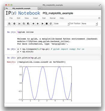
An IPython notebook is an analog to running commands in terminal-based IPython, but using a web browser window (Shen, 2014). Python commands and their results can be saved for future communication and collaboration. To start IPython in this mode, type ipython notebook in the command line on your computer. An IPython notebook is comparable to a spreadsheet with only a single column, but where each cell can contain formatted text or Python code, optionally accompanied with output from the previous commands. As shown in Figure 3, output may contain graphics and plots embedded within the notebook.
(Color online) An example of a computation performed in an IPython notebook showing a simple computation and the graphed result. The IPython notebook file can be shared by e-mail or even within a network, with a secured server.
Hence, an IPython notebook is an excellent way for:
-
• researchers to collaborate on data analysis,
-
• instructors to provide worked-through examples of computations and perhaps even homework or exam problems,
-
• speakers to showcase Python code within their slides in their talks or workshops.
Normally, the IPython notebook web service can only be accessed from the computer where the process is started. With appropriate security protections in place, an IPython notebook server could allow individuals to attack a programming or data analysis problem as a team with all members of the team running Python from the same server using IPython via a web browser. An IPython notebook likewise can be used within a classroom setting to allow a group of students to work collaboratively with Python without having to install the interpreter on their individual computers. There are also free and commercial services that offer access to IPython notebooks over the web, such as Wakari (https://www.wakari.io/wakari). Notebooks can also be freely viewed via the nbviewer service (http://nbviewer.ipython.org/), by entering a link to your gitlab or github repository or a link to your own website that hosts the notebook. The IPython sponsored Jupyter CoLaboratory (https://colaboratory.jupyter.org/welcome/) project allows real-time editing of notebooks, and currently uses Google Drive to restrict access to users with shared permissions.
As an example of how IPython can be used to share a worked-through problem, the computations in the “Performing efficient computations with NumPy” section, above, are provided at this URL (https://anl.box.com/s/hb3ridp66r247sq1k5qh) and the Supplementary Materials, which also includes IPython notebook files demonstrating several other code examples along with their output.
VIII. CONCLUSIONS
As we have discussed and demonstrated here, Python is a powerful programming language, although simple enough to be taught in introductory high school courses. It can be learned easily, but still offers tremendous power for professional software development. The large wealth of scientific packages, of which only a few were presented here, shows the high value that Python has in the hands of scientists. The authors encourage scientists to learn and use Python in their own work.
ACKNOWLEDGEMENTS
Use of the Advanced Photon Source, an Office of Science User Facility operated for the US Department of Energy (DOE) Office of Science by Argonne National Laboratory, was supported by the US DOE under Contract no. DE-AC02-06CH11357. The authors of this manuscript have never met in person and all collaboration was done exclusively via the internet text services (e-mail, git DVCS, bug tracking, etc.). Text formatting was done using the Markdown protocol and drafts were tracked using Git for version control. The authors thank the websites CloudHost.io (now defunct) and GitLab.com for providing the DVCS web services that made this manuscript a reality.
SUPPLEMENTARY MATERIALS AND METHODS
The supplementary material for this article can be found at http://www.journals.cambridge.org/PDJ
Appendix 1: A Brief Introduction to Python
Presenting the full syntax of Python is beyond the scope of this paper, but here we provide some basic information about how Python code is written and some background information on the differing versions of the interpreter.
A1.1 Python statements and syntax
Probably the most basic statement in any language is that of assignment of a value to a variable. In Python, this is straightforward and no declarations for the type of information in a variable are required:
Note that in these assignments, variables a, b, and c, are assigned in turn, an integer, character, and floating-point value.
However, unlike C/C ++ or Java, in Python the types associated with a variable are never declared explicitly, rather the type is associated with the value (or object) stored in that variable. The type can then change as the contents of a variable is reassigned. A strength of Python is a concept called duck typing (from the joke that if an object walks like a duck, quacks like a duck, and then consider it a duck). One writes code that will process values without knowing the details of the object type. The statement,
increments the value in variable a by 1, where this can be applied to an integer, float, or complex value or with NumPy increments every element in an array. If a contains a string, an error condition occurs, but Python provides a mechanism for trapping that (commands try and except) so that an appropriate response can be taken.
Many types of Python objects contain collections of other values (for example, the string “one” above is a collection of three letters). Two other examples are the composite data types of “lists” and “dicts” that can each contain multiple values:
In the example above, list d, contains six-ordered values, where the first, which can be referenced as d[0], is 1 and the last, which can be referenced as d[5] or d[-1], is 11.
The dict in the second line, e, is a kind of array, but where values are located by arbitrary keys, so in the above, e[2] is defined with a value of 4, but no value for e[1] has been defined. Note that above, three of the keys are integers, but one is a string ('primes') and the value associated with that element references another composite item (list d).
Values can be added to a dict or list and the contents can be changed:
Since the value associated with key 'primes' in dict e directly references list d, changes to d will affect e; likewise changes to e['primes'] can affect d.
When a variable name is placed on a line by itself in a script, nothing happens, but when this is done in interactively, the interpreter shows the contents of the variable, as is shown above. Note also that the order that Python lists keys for a dict is arbitrary, so you may see the contents of e in a different order than shown above, if you repeat this example.
All computer languages have methods for conditional execution. In Python, the if statement is particularly simple, where one creates an if clause that ends with a colon (“:”), as shown here:
The example above shows several important Python features. Note that the block nature of the code is indicated by the indentation, where two statements are to be run when the if statement evaluates as true or one statement if false. The if statement ends where the code matches the original level of indentation. Blocks can be nested, with multiple levels of indentation, when an if statement appears within an if block. The amount of indentation is arbitrary, as long as all lines in the block are indented the same, but it is strongly recommended that four spaces be used for each level of indentation. Parentheses are allowed in the if statement, but are only required when needed for correct logical formulation of the test:
The above statement will test as true anytime that c is 3, whereas the test below will always be False if a is not 1.
There are several types of statements in Python that execute a set of lines of code multiple times, a concept called looping. The most commonly used one is the for statement, which will execute the code for every value in a collection. As another example of duck typing, the for statement can be used with nearly every composite data type, including dict, list, or even character string values to access each element:
In the above example, we use a Python function, range(), which when called with argument 4 generates a list, [0,1,2,3], but we could have also looped over values in d with for v in d:, which would cause v to be set sequentially to values 1, 2, 3,…, 17. Likewise, we could loop over the dict e with for v in e:, which would cause v to be set to the values corresponding to the keys in the dict, here 0, 2, 3, 4 and “primes”, but note that since dicts are not ordered, the order each key will be referenced cannot be predicted.
As an example, where looping and an if statement are combined, consider:
Here, note how multiple levels of indentation are used, where the if statement is inside the loop and the “print” statement is inside the if conditional statement. If other statements were to be included inside the loop, to be run after the if statement is completed, those statements would be indented to match the if statement, for example:
To complete our Python syntax introduction, we show how to create a function; noting that user-written functions are used identically to the many built-in functions. The function is created with a def statement:
Indentation indicates the end of block of code used to define the function. Note that the first line of code after the def statement defines a string, but nothing is done with that string, so it has no effect on the code. Such a string, when supplied as the first line of a function definition, is called a docstring and by convention it provides documentation on the function.
A1.2 Documenting Python code
Documentation is essential for computer software. It allows code to be reused or fixed by others. In fact, even the original author can benefit, should that person work on something else, take a vacation, get sick, etc., and then need a reminder of what they have done. Python offers a nice tool called Sphinx (http://sphinx-doc.org/) for creating documentation from the docstrings in Python code (Brandl, Reference Brandl2010). To use it, a description is included in a docstring for every function and class to be included in that documentation. These comments can be formatted using reStructured Text (http://sphinx.pocoo.org/rest.html), which allows for various types of useful cross-references, changes in fonts, headers, etc. Sphinx is then be used to build documentation files in a variety of formats, including HTML and PDF. Sphinx is used for the online Python and NumPy documentation, which is very usefully and attractively displayed.
Programmers are advised to always follow some very simple rules in adding comments to the definitions of their code no matter how rudimentary. At a minimum, for every function, include a docstring that defines what the function does:
To better use Sphinx, keywords param and returns are used to document the input and output, as below. Note that we have also snuck in an example of a cross-reference keyword (:func:). When Sphinx generates documentation, this would render a link to the description of function grunge, if present. The keyword str in the first :param: definition is an optional data type, which is wise to include if a programmer should know what data type is expected for that parameter.
It is good practice to always document their program code, even for a simple and obvious program so that if that code finds its way into a larger project, where good documentation becomes a necessity, the project will be ready for Sphinx with minimal added effort.
A1.3. Python versions
All computer languages evolve with use, where capabilities added in the later stages will be absent in earlier versions, so there is always the potential for incompatibilities. The Python language has been evolving and growing for over two decades and in most cases where new features have been added to the language, this is done with backward compatibility to ensure that code that ran in an earlier version of Python will run completely unchanged in a newer version. An exception to this is Python 3.0 and subsequent versions, which was intended to eliminate design flaws in the original version of the language. (We will refer to the new Python series as 3.x and the previous version as 2.7.) Python 3.x did introduce some minor changes in the language that are incompatible with syntax originally allowed. Other coding practices in Python have been indicated as depreciated – meaning that their use is discouraged and at some point these features may be removed from the language. As one example, in Python 3.x, the preferred use of the print statement is print(line), while in the original language this was written as print line. In both Python 2.7 and 3.x, both syntaxes are allowed. Indeed, the updates both required and recommended in Python 3.x, are all allowed in Python 2.7, so the same code can be used in both. At some point in the future, (Python 4?) perhaps the old style print might trigger a warning.
Since most of the coding changes for Python 3.x are easy to recognize and fix, they can be made automatically with a program called 2to3, which is distributed with Python. An alternative to that is Six (http://pythonhosted.org/six/), which is built on the core “lib2to3” package and offers additional support for refactoring Python code.
While this transition has caused some community alarm that working Python software might suddenly break, the change is really a long-term strategy. Both Python 2.7 and 3.x interpreters are still being updated; the latest versions (at the time this is being written) are Python 2.7.8 (released on July 1, 2014) and Python 3.4.2 (released on October 6, 2014.) Updates to address bugs in Python 2.7 are planned to continue at least through 2020, while in parallel a Python 3.5 upgrade, which will add new features is also in progress.
Appendix 2: Resources for Learning Python
While a formal course on Python may be a good way to learn a first or a new programming language, not everyone has access to, or the time for, or even the preference for that mode of learning. Even after learning the basics of Python, there are a wide variety of highly advanced skills that can benefit scientists, even ones actively using Python in their daily work. Fortunately, there are many other resources available for learning the use of Python. Below, we provide many Python resources that we feel are of particular value to scientists wishing to learn the language or tools for scientific programming.
A2.1 Community events
The Python community is large and there are many events and groups with a scientific focus. There are user groups and conferences where community members meet and attend talks, workshops, tutorials, and perform-coding sprints. In-person events are an excellent learning resource and some interesting events and useful resources are listed below:
-
• SciPy Conferences (http://conference.scipy.org/) is a yearly conference highly focused on scientific programming.
-
• PyData (http://pydata.org/) is an event and conference focused on data analysis.
-
• Python Conferences and Workshops (https://www.python.org/community/workshops/) are python events with a general focus.
-
• Python User Groups (https://wiki.python.org/moin/LocalUserGroups) lists regional user groups, which have a variety of events, mailing lists, etc.
-
• OpenHatch Events (https://openhatch.org/events/) runs workshops focused toward beginning programmers.
A2.2 Mailing lists and help sites
There are a number of e-mail mailing lists related to Python and most widely used packages also have their own mailing lists. Many experienced and dedicated Python users read the postings actively and it can be quite common to get a quick helpful response to a very specialized question. Local user groups may also run very useful mailing lists. However, a few precautions are in order:
-
• Spend some time-reading messages on the list before posting. Most mailing lists have archives and searching for a previously posted question rather than asking it again can save everyone's time.
-
• There are many preferred styles that are used for different lists. For example, on some lists, people will be annoyed when replies are top-posted, while on other lists it may be the preferred format. Read the archives to observe and follow the predominant style for the list you are posting messages to.
-
• Posting a large program and asking for help with a problem in that code rarely generates a useful outcome. It takes work to prepare, but a short example (typically 10–25 lines of code) can typically demonstrate a problem in a manner that can be quickly read and understood. Such short examples are much more attractive to the cognoscenti to browse. Also, note that inclusion of Python code in the text of an e-mail almost invariably results in a loss of the indentation that Python requires. Code examples or output errors are best posted on a github gist or other free sites (such as dpaste.de, pastebin.com) that allow you to share snippets of code. The resulting hashed link should be included in your email query to the mailing list. Attachments containing small amounts of code are encouraged on some mailing lists, but are not allowed on others.
-
• Finally, on mailing lists it is important to be polite and helpful. Remember that anyone reading and responding to you is doing so as a volunteer and simply for the pleasure of helping. People who are annoying make the process much less of a pleasure.
A related form of help can be found on wiki sites and similar self-help sites, of which Stackoverflow (stackoverflow.com) seems to be the most widely used. The goal here is that a question is raised and different people may suggest answers. Readers score the answers, so the best one(s) are usually top rated. Repeating a previous question in this type of forum is frowned upon. Search engines are generally the best way to find previously asked questions.
A2.3 Web institutions
Organizations that promote best practices in software and data management for scientists also run events and make lessons and videos available online; these can also be directly useful to scientists learning to program.
-
• Software Carpentry (http://software-carpentry.org) provides lessons and bootcamps on which are structured to teach scientists command line and programming skills that make their work more productive. Lesson materials are maintained in a repository (https://github.com/swcarpentry/bc) and published to the Software Carpentry website, Programming with Python: Introduction to data analysis and programming with Python (http://software-carpentry.org/v5/novice/python/index.html).
-
• Data Carpentry (http://datacarpentry.org/) is a Software Carpentry offshoot with an intense focus on data analysis skills. Data Carpentry materials are also maintained in a public repository (https://github.com/datacarpentry/datacarpentry).
-
• The Software Sustainability Institute (http://www.software.ac.uk/) works in conjunction with these groups and others to promote practices that lead toward usable and maintainable research software. They provide materials, run events, and offer training.
A2.4 Interactive tutorials/references
A number of websites offer interactive Python tutorials, which can be another resource for people wanting to learn programming skills. Some of these are based around textbooks, but all offer free access to at least some of the material:
-
• CodingBat Python (http://codingbat.com/python);
-
• How to Think Like a Computer Scientist (http://interactivepython.org/runestone/static/thinkcspy/index.html);
-
• Learn Python (http://www.learnpython.org/);
-
• Online Python Tutor: Learn programming by visualizing code execution (http://www.pythontutor.com/);
-
• Problem Solving with Algorithms and Data Structures (http://interactivepython.org/runestone/static/pythonds/index.html);
-
• Python Codecademy (http://www.codecademy.com/tracks/python);
-
• Learn Python the Hard Way (http://learnpythonthehardway.org/book/);
-
• Introduction to Python for Science (https://github.com/djpine/pyman): an electronic book aimed at students;
-
• Python Scientific Lecture Notes (https://scipy-lectures.github.io/): notes for professional scientists.
A2.5 Online courses
Many educational institutions have begun offering massive open online courses (MOOCs), which usually allow some form of participation without charge, although providers do charge for grading, certification, etc. Some examples of Python course offerings from some courseware providers are listed below. Note that course offerings change at the discretion of the providers, and some place materials online only when the class is being run, so some of these listings may not be available at any given time.
-
• A Gentle Introduction to Python (http://mechanicalmooc.org/);
-
• High Performance Scientific Computing (https://www.coursera.org/course/scicomp);
-
• An Introduction to Interactive Programming with Python (https://www.coursera.org/course/interactivepython);
-
• Introduction to Computer Science and Programming Using Python (https://www.edx.org/node/2841);
-
• Programming Foundations with Python (https://www.udacity.com/course/ud036);
-
• Python for Informatics: Exploring Information (http://pythonlearn.com/), related MOOC site is Programming for Everybody (https://www.coursera.org/course/pythonlearn);
-
• List of free online programming and computer courses (https://github.com/fffaraz/free-programming-courses).
While not a complete course, the paid subscription versions of the Python bundle offered by Enthought, Inc., Canopy (https://www.enthought.com/products/canopy/), provides access to downloadable training lectures that include many topics of interest to scientists. Enthought offers academic users (students and faculty) free access to their products, including these lectures.
A2.6 Curated web resources
A number of individuals provide annotated lists of resources for Python programmers. These crowd-sourced efforts can be the most up-to-date sources of information about available packages, books, and other materials. The maintainers of these lists and update them on a regular basis and the maintainers will likely appreciate hearing about broken or changed URLs, as well as suggestions of additional resources.
-
• Python for Non-Programmers (https://wiki.python.org/moin/BeginnersGuide/NonProgrammers): resources for beginning programmers.
-
• Pythonidae (http://svaksha.github.io/pythonidae) contains curated descriptions of scientific programming resources in Python.
-
• Awesome-python (https://github.com/vinta/awesome-python) has a curated list of awesome Python frameworks, libraries and software.
-
• Planet SciPy (http://planet.scipy.org/) aggregates blog posts from the scientific Python community.
-
• Planet Python (http://planet.python.org/) aggregates blog posts from the overall Python community.
-
• pyvideo.org (http://pyvideo.org/) indexes Python videos of conferences, lectures, tutorials, and events.
-
• List of free programming books (https://github.com/vhf/free-programming-books)
-
• List of free software testing books (https://github.com/ligurio/free-software-testing-books)
-
• The Python Bookshelf (https://github.com/OpenTechSchool/bookshelf/blob/master/python.md)


