


Impact Statement
Traditional theories of non-uniform sediment transport attribute the preferential entrainment of coarse particles to their greater exposure and increased hydrodynamic drag—a phenomenon known as the “exposure effect.” Our study extends this framework by revealing a previously unrecognized mechanism: even under identical exposure conditions, coarse particles experience significantly higher Reynolds shear stresses than finer particles due to permeability-induced flow heterogeneity. We demonstrate that spatial variability in bed permeability, along with the emergence of cross-sectional secondary flows, plays a pivotal role in redistributing shear stresses and modulating bed resistance at the particle scale. These findings offer new theoretical insight into the mechanisms underlying the preferential entrainment of coarse particles and support the development of more accurate sediment transport models for heterogeneous beds.
1. Introduction
Riverbed sediment coarsening, resulted from the replacement of original riverbed substrates with larger sediments particles, is a fluvial process frequently observed downstream of dams or in areas with a high abundance of benthos (McLachlan Reference McLachlan1996; De Backer et al. Reference Rhoads, Yingst, Ullman and Wiley2011; Rhoads et al. Reference De Backer, Van Coillie, Montserrat, Provoost, Van Colen, Vincx and Degraer1978; Krasnow & Taghon Reference Krasnow and Taghon1997; Li et al. Reference Li, Ni, Chang, Yue, Frolova, Magritsky, Borthwick, Ciais, Wang, Zheng and Walling2020; Cardinale et al. Reference Cardinale, Palmer, Swan, Brooks and Poff2002). For example, the release of freshwater downstream of dams leads to resuspension of fine sediments while leaving coarser grains retained on the riverbed (Zhou et al. Reference Zhou, Lu, Jin, Li, Gao, Liu and Chen2021). Additionally, benthos aggregate fine sediments into larger spherical or subspherical clusters on the riverbeds as a mean of habitat protection (De Backer et al. Reference De Backer, Van Coillie, Montserrat, Provoost, Van Colen, Vincx and Degraer2011; Krasnow & Taghon Reference Krasnow and Taghon1997; Mason et al. Reference Mason, Rice, Wood and Johnson2019). During the process of riverbed sediment coarsening, bed shear stress and flow resistance increase, which enhances flow exchange across the sediment–water interface (SWI) (Dancey et al. Reference Dancey, Balakrishnan, Diplas and Papanicolaou2000). This modification can alter the transport rates of key scalars, such as dissolved oxygen and silicate, (Xiao et al. Reference Xiao, Wu, Pan, Huang, Peng, Lu and Santos2024; Fang et al. Reference Fang, Han, He and Dey2018), potentially impacting the ecological and hydrological dynamics of aquatic systems.
In a flow over uniform riverbed substrates, sediment size plays a crucial role in governing the near-bed hydrodynamics. Larger sediment sizes typically result in greater equivalent roughness heights (Van Rijn Reference Van Rijn1984a). This leads to reduced near-bed streamwise velocities (Mazzuoli & Uhlmann Reference Mazzuoli and Uhlmann2017), larger turbulence structures (Han et al. Reference Han, Fang, He and Reible2018), increased turbulent kinetic energy (Lazzarin et al. Reference Lazzarin, Cameron, Stamhuis, Martin, Erftemeijer, Nikora and Uhlmann2023) and stronger flow resistance (Van Rijn Reference Van Rijn1984b). The impact of sediment size on the time-averaged flow velocity ( $\overline{u}$
) is typically quantified through the roughness coefficient (
$\overline{u}$
) is typically quantified through the roughness coefficient ( $B_{s}$
) in the logarithmic velocity profile (Da Silva & Yalin Reference Da Silva and Yalin2017)
$B_{s}$
) in the logarithmic velocity profile (Da Silva & Yalin Reference Da Silva and Yalin2017)
 \begin{equation}\overline{u}/u_{*}=1/\kappa \ln (z/k_{s})+B_{s},\end{equation}
where $u_{*}$
is the friction velocity,
$u_{*}$
is the friction velocity, $\kappa$
is the von Kármán constant,
$\kappa$
is the von Kármán constant, $z$
is the distance from the channel bed and
$z$
is the distance from the channel bed and $k_{s}$
is the roughness height. The value of
$k_{s}$
is the roughness height. The value of $B_{s}$
initially increases with sediment size when substrate tops are submerged within the viscous sublayer, reaching a local maximum when sediment size is comparable to the viscous sublayer thickness. Beyond this point,
$B_{s}$
initially increases with sediment size when substrate tops are submerged within the viscous sublayer, reaching a local maximum when sediment size is comparable to the viscous sublayer thickness. Beyond this point, $B_{s}$
drops slightly and stabilises at 8.5 as the sediment size exceeds the sublayer thickness (Da Silva & Yalin Reference Da Silva and Yalin2017). Furthermore, Nikora et al. (Reference Nikora, Stoesser, Cameron, Stewart, Papadopoulos, Ouro, McSherry, Zampiron, Marusic and Falconer2019) provided evidence that larger riverbed sediments enhance flow resistance primarily due to increased dispersive Reynolds shear stress.
$B_{s}$
drops slightly and stabilises at 8.5 as the sediment size exceeds the sublayer thickness (Da Silva & Yalin Reference Da Silva and Yalin2017). Furthermore, Nikora et al. (Reference Nikora, Stoesser, Cameron, Stewart, Papadopoulos, Ouro, McSherry, Zampiron, Marusic and Falconer2019) provided evidence that larger riverbed sediments enhance flow resistance primarily due to increased dispersive Reynolds shear stress.
The heterogeneity of bed substrates is another key factor influencing the near-bed hydrodynamics. Compared with flows over uniform channel beds, turbulence-driven secondary currents (SCs) are notably prominent above heterogeneous bed configurations featuring alternating smooth and rough strips (Blanckaert et al. Reference Blanckaert, Duarte and Schleiss2010; Stoesser et al. Reference Stoesser, McSherry and Fraga2015). The dimensions of these SCs are determined by the spatial characteristics of the strips, while the intensity is influenced by the roughness height ratio of rough to smooth strips. These SCs enhance bed shear stress over the rough strips, resulting in an approximate doubling of the reach-averaged bed shear stress (Stroh et al. Reference Stroh, Schäfer, Frohnapfel and Forooghi2016).
The hyporheic exchange, referring to the flow exchange between surface currents and subsurface interstitial flows, is also significantly influenced by the size and heterogeneity of riverbed substrates. Increased bed roughness and substrate heterogeneity have been found to intensify macro-scale turbulent structures and SCs, and strengthen local dowelling flow (Boano et al. Reference Boano, Harvey, Marion, Packman, Revelli, Ridolfi and Wörman2014; Han et al. Reference Han, Fang, He and Reible2018; He et al. Reference He, Han, Fang, Reible and Huang2019). These effects enhance turbulent diffusion around the SWI, leading to higher rates of vertical scalar transport. Observations indicated that greater bed surface heterogeneity and roughness promote deeper penetration of passive substances, such as dissolved oxygen, into the subsurface (Boano et al. Reference Boano, Harvey, Marion, Packman, Revelli, Ridolfi and Wörman2014; He et al. Reference He, Han, Fang, Reible and Huang2019; Liu et al. Reference Liu, Wallace, Zhou, Ershadnia, Behzadi, Dwivedi, Xue and Soltanian2020). Previous studies on hyporheic exchange have primarily focused on its effects on water and solute fluxes at the SWI, as well as the subsequent biogeochemical processes (Dudunake et al. Reference Dudunake, Tonina, Reeder and Monsalve2022; Lee et al. Reference Lee, Aubeneau, Cardenas and Liu2022). Very little is known on the effects of hyporheic momentum exchanges on the hydraulic resistance, although few studies (e.g. Manes et al. Reference Manes, Pokrajac, Nikora, Ridolfi and Poggi2011) suggest that they be significant.
Despite numerous studies demonstrating that, under identical Reynolds numbers, increasing bed particle dimensions leads to an increase in roughness height and drag coefficient (Fang et al. Reference Fang, Han, He and Dey2018; Han et al. Reference Han, Fang, He and Reible2018; He et al. Reference He, Han, Fang, Reible and Huang2019), in natural rivers, the replacement of finer sediments by coarser materials typically occurs locally and evolves in time (Zhou et al. Reference Zhou, Lu, Jin, Li, Gao, Liu and Chen2021). This process results in the formation of patchy distributions of coarse particles, with the coverage of coarser sediments on the riverbed gradually increasing (Fan et al. Reference Fan, Zhong, Nie and Liu2023; Li et al. Reference Li, Saletti, Hassan, Johnson, Carr, Chui and Yang2023). This suggests that the ratio of the riverbed area that occupied by coarser sediments (A c) to the total riverbed area (A t) (denoted as A c/A t, hereafter referred to as the ‘coverage ratio’) can vary continuously between 0 % and 100 %. The effects of varying coarse particle coverage on the near-bed hydrodynamics and reach-averaged flow resistance remain poorly understood. In addition, coarsening introduces heterogeneity in internal bed structures, such as permeability and porosity, which has received little attention. In scenarios where finer and coarser particles share the same crest elevations, the impact of heterogeneous permeability on the near-bed hydrodynamics may be even more significant than that of bed roughness coarsening.
To gain a comprehensive understanding of the impact at various stages of coarsening on both bed roughness and permeability, six numerical simulations with different coverage ratios are performed: A c/A t = 0 % (uncoarsened scenario), 4 %, 16 %, 36 %, 64 %, (partially coarsened scenario) and 100 % (fully coarsened scenario).The main objectives of this study are to address the following questions: (i) What are the differences in time-averaged velocity, Reynolds shear stress and hyporheic exchange across different coverage ratios? (ii) How does the replacement of finer sediments with coarser sediments affect global bed shear stress? (iii) What mechanisms drive the observed alterations in global bed shear stress?
2. Method
2.1. Governing equations
Large-eddy simulation (LES) is applied via the code Hydro3D, which has been validated in several flows of similar complexity (Liu et al. Reference Liu, Reible, Hussain and Fang2019, Reference Liu, Stoesser and Fang2022a, Reference Liu, Stoesser and Fang2022b; Ouro et al. Reference Ouro, Fraga, Lopez-Novoa and Stoesser2019). The code is based on finite differences applied on a staggered Cartesian grid and solves the filtered NavierStokes equations for incompressible flow:
 \begin{equation}\frac{\partial u_{i}}{\partial x_{i}}=0,\end{equation}
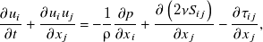 \begin{equation}\frac{\partial u_{i}}{\partial t}+\frac{\partial u_{i}u_{j}}{\partial x_{j}}=-\frac{1}{{\unicode[Arial]{x03C1}} }\frac{\partial p}{\partial x_{i}}+\frac{\partial \left(2\nu S_{ij}\right)}{\partial x_{j}}-\frac{\partial \tau _{ij}}{\partial x_{j}},\end{equation}
where u i is the filtered velocity (i represents x, y and z coordinates); ${\unicode[Arial]{x03C1}}$
is the water density; p is the pressure; ʋ is the kinematic viscosity; and
${\unicode[Arial]{x03C1}}$
is the water density; p is the pressure; ʋ is the kinematic viscosity; and $S_{ij}$
is the strain-rate tensor. The sub-grid-scale (SGS) stress is defined as
$S_{ij}$
is the strain-rate tensor. The sub-grid-scale (SGS) stress is defined as $\tau _{ij}=-2\nu _{t}S_{ij}$
, where
$\tau _{ij}=-2\nu _{t}S_{ij}$
, where $\nu _{t}$
is the eddy viscosity, and in this study the wall-adapting local eddy viscosity proposed by Nicoud and Ducros (Reference Nicoud and Ducros1999) is used to compute the SGS stress.
$\nu _{t}$
is the eddy viscosity, and in this study the wall-adapting local eddy viscosity proposed by Nicoud and Ducros (Reference Nicoud and Ducros1999) is used to compute the SGS stress.
The advection and diffusion terms in the Navier–Stokes equations are estimated by fourth-order accurate central differences. An explicit 3-step Runge–Kutta scheme is used to integrate in time, providing second-order accuracy. A fractional step method is applied within the time step, and convection and diffusion terms are solved explicitly first in a predictor step which is then followed by a corrector step during which the pressure and divergence-free velocity fields are obtained through a Poisson equation. The latter is solved iteratively through a multi-grid procedure (Ouro et al. Reference Ouro, Fraga, Viti, Angeloudis, Stoessor and Gualtieri2018, Reference Ouro, Fraga, Lopez-Novoa and Stoesser2019).
2.2. Numerical set-ups
Figure 1 presents the domain and the set-up of the simulations. The water depth (h) is 5 cm and the computational domain of the simulation spans L x = 24h in the streamwise, L y = 6h spanwise and L z = 2h vertical directions. The channel bed is filled with five layers of cubic packed finer spheres of diameter d = 1 cm in the uncoarsened scenario (case 1) and by three layers of coarser spheres of diameter D = 2 cm in the fully coarsened scenario (case 6). These sphere sizes are representative of riverbed sediments in the Yangtze River before and after the construction of the Three Gorges Dam, respectively (Zhou et al. Reference Zhou, Lu, Jin, Li, Gao, Liu and Chen2021). For the partially coarsened scenarios (cases 2 to 5), finer spheres are replaced with coarser spheres in a patch-like configuration with uniform spacing between patches (Figure 1). Each patch contains $N\times N$
coarser spheres, where
$N\times N$
coarser spheres, where $N$
increases progressively from 1 to 4 across cases 2 to 5. This results in a corresponding increase in the coverage ratio, ranging from 4 % to 64 %. The elevations of the crest of all spheres are kept identical, collectively defining the roughness top (z = 0).
$N$
increases progressively from 1 to 4 across cases 2 to 5. This results in a corresponding increase in the coverage ratio, ranging from 4 % to 64 %. The elevations of the crest of all spheres are kept identical, collectively defining the roughness top (z = 0).
Computational domain of the LES. The blue longitudinal plane in (c) represents the plane located midway between adjacent arrays of coarser spheres, hereafter referred to as the ‘void plane’. The red plane in (d) represents the plane passing through the centres of coarser spheres, hereafter referred to as the ‘core plane’. Note that, in case1, the void and core planes correspond to the longitudinal planes through the interspace and centres of the finer spheres, respectively.
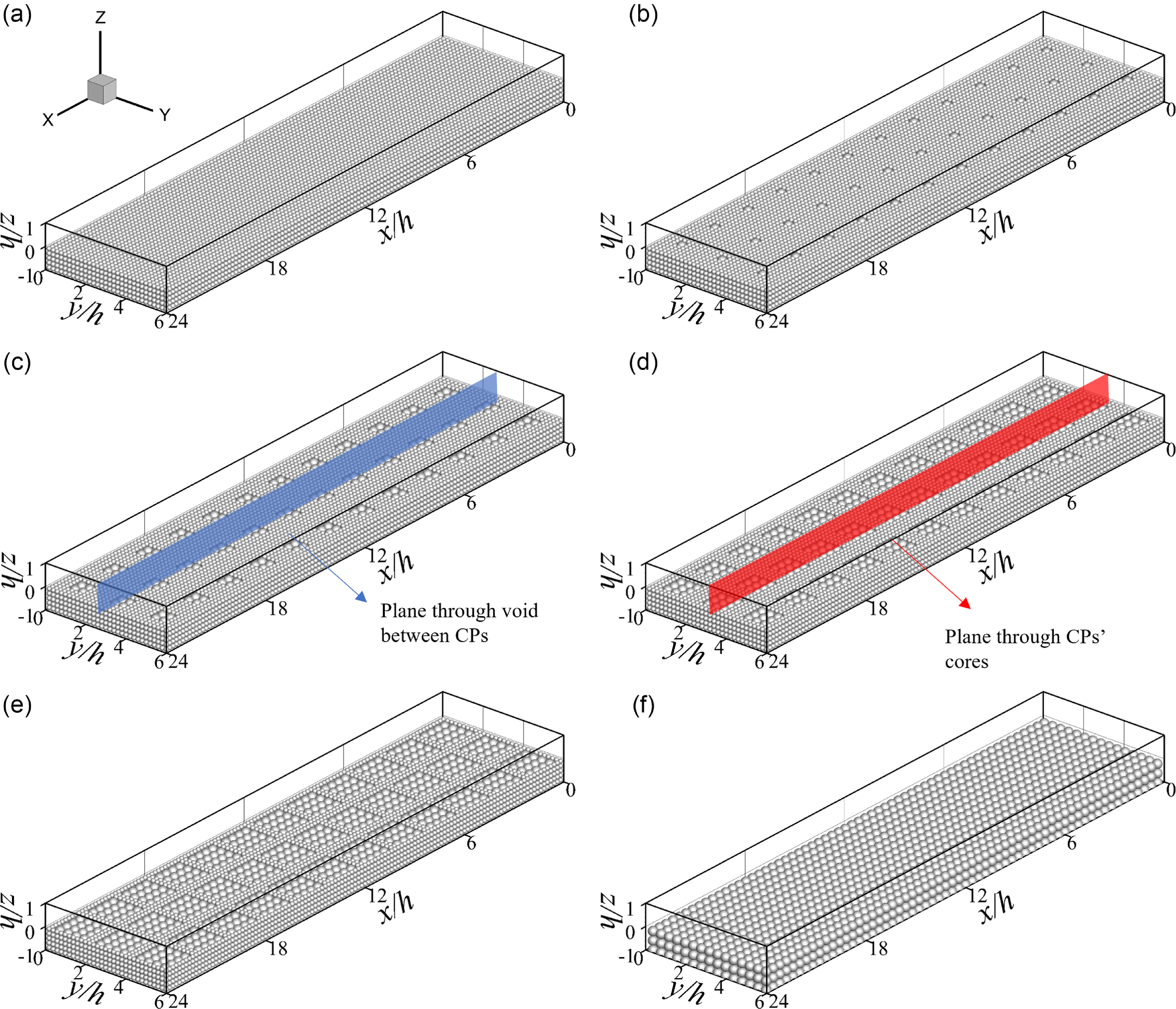
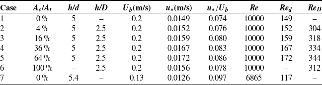
Table 1 summarises the hydraulic background conditions of the simulations. In total, eight simulations with different coverage ratios of coarser particles ranging from 0 % to 100 % are performed. For cases 1 to 6, the water depth and the bulk flow velocity ( $U_{b}$
), referring to the depth-averaged velocity above particle tops, are maintained constant, leading to an identical Reynolds number of 10000 (defined as
$U_{b}$
), referring to the depth-averaged velocity above particle tops, are maintained constant, leading to an identical Reynolds number of 10000 (defined as $Re=U_{b}h/\upsilon$
). Case 7 serves as a validation case based on the direct numerical simulation conducted by Mazzuoli and Uhlmann (Reference Mazzuoli and Uhlmann2017), the data of which are used to validate the LES. In cases of flows over permeable beds, a friction velocity can be defined in several ways, including: (i) a friction velocity based on the water depth over roughness tops, given by
$Re=U_{b}h/\upsilon$
). Case 7 serves as a validation case based on the direct numerical simulation conducted by Mazzuoli and Uhlmann (Reference Mazzuoli and Uhlmann2017), the data of which are used to validate the LES. In cases of flows over permeable beds, a friction velocity can be defined in several ways, including: (i) a friction velocity based on the water depth over roughness tops, given by $u_{*}=\sqrt{gSh}$
(Manes et al. Reference Manes, Pokrajac, Nikora, Ridolfi and Poggi2011), where
$u_{*}=\sqrt{gSh}$
(Manes et al. Reference Manes, Pokrajac, Nikora, Ridolfi and Poggi2011), where $S$
is the bed slope, (ii) a friction velocity based on the effective height of water column in both the surface and hyporheic regions and g is acceleration of gravity, expressed as
$S$
is the bed slope, (ii) a friction velocity based on the effective height of water column in both the surface and hyporheic regions and g is acceleration of gravity, expressed as $u_{*}=\sqrt{gS(h+\mathrm{\varnothing }h_{h})}$
(Manes et al. Reference Manes, Pokrajac, Nikora, Ridolfi and Poggi2011), where
$u_{*}=\sqrt{gS(h+\mathrm{\varnothing }h_{h})}$
(Manes et al. Reference Manes, Pokrajac, Nikora, Ridolfi and Poggi2011), where $\mathrm{\varnothing }$
and
$\mathrm{\varnothing }$
and $h_{h}$
are the averaged porosity and the height of the hyporheic region, respectively, and (iii) a friction factor based on the extrapolation of the linear profile of wall-normal total shear stress to the virtual bed height (z 0) (Mazzuoli & Uhlmann Reference Mazzuoli and Uhlmann2017). In the current simulations, both
$h_{h}$
are the averaged porosity and the height of the hyporheic region, respectively, and (iii) a friction factor based on the extrapolation of the linear profile of wall-normal total shear stress to the virtual bed height (z 0) (Mazzuoli & Uhlmann Reference Mazzuoli and Uhlmann2017). In the current simulations, both $h_{h}$
and z 0 are expected to vary with different coverage ratios (A c/A t) and are not known a priori. Consequently, the friction velocity based on the water depth over roughness tops is adapted and calculated as
$h_{h}$
and z 0 are expected to vary with different coverage ratios (A c/A t) and are not known a priori. Consequently, the friction velocity based on the water depth over roughness tops is adapted and calculated as $u_{*}=\sqrt{-\frac{h}{\rho }\left\langle \frac{dp}{dx}\right\rangle }$
, where
$u_{*}=\sqrt{-\frac{h}{\rho }\left\langle \frac{dp}{dx}\right\rangle }$
, where $\left\langle \frac{dp}{dx}\right\rangle$
is the pressure gradient that drives the flow. Particle Reynold numbers based on the diameter of the finer (
$\left\langle \frac{dp}{dx}\right\rangle$
is the pressure gradient that drives the flow. Particle Reynold numbers based on the diameter of the finer ( $Re_{d}=u_{*}d/\upsilon$
) and coarser spheres (
$Re_{d}=u_{*}d/\upsilon$
) and coarser spheres ( $Re_{D}=u_{*}D/\upsilon$
) are also provided in Table 1.
$Re_{D}=u_{*}D/\upsilon$
) are also provided in Table 1.
Hydraulic conditions of all cases
Meshes applied for all simulations are given in Table 2. A uniform grid is applied for the validation case (case 7) with grid points 960 × 480 × 160 in the streamwise, spanwise and vertical directions, respectively. Stretched grids are used in cases 1 to 6 due to the significantly larger domain size. The mesh comprises 1200 × 400 × 200 grid points in the x-, y- and z- directions, respectively. The grid resolutions away from the spheres are ${\Delta} x^{+} = {\Delta} y^{+} = {\Delta} z^{+}$
= 8.32 for the validation case and
${\Delta} x^{+} = {\Delta} y^{+} = {\Delta} z^{+}$
= 8.32 for the validation case and $0.5{\Delta} x^{+} = 0.5{\Delta} y^{+} = {\Delta} z^{+}$
=7.44 - 8.58 for the other cases, where the normalised grid spacing is calculated as
$0.5{\Delta} x^{+} = 0.5{\Delta} y^{+} = {\Delta} z^{+}$
=7.44 - 8.58 for the other cases, where the normalised grid spacing is calculated as ${\Delta} ^{+}=u_{*}{\Delta} /\upsilon$
. For near-wall grids, the resolution is determined based on the averaged normal distance from the first fluid grid points to the sphere surface (
${\Delta} ^{+}=u_{*}{\Delta} /\upsilon$
. For near-wall grids, the resolution is determined based on the averaged normal distance from the first fluid grid points to the sphere surface ( ${\Delta} _{w}$
), which is approximately 43 % of the largest fluid grid spacing
${\Delta} _{w}$
), which is approximately 43 % of the largest fluid grid spacing ${\Delta} x$
as shown in Liu et al. (Reference Liu, Tang, Huang, Stoesser and Fang2024). Giving this, the near-wall grid resolutions are calculated as
${\Delta} x$
as shown in Liu et al. (Reference Liu, Tang, Huang, Stoesser and Fang2024). Giving this, the near-wall grid resolutions are calculated as ${\Delta} _{w}^{+}=u_{*}{\Delta} _{w}/\upsilon$
, ranging from 6.40 to 7.38 for cases 1 to 6, and 3.58 for the validation case.
${\Delta} _{w}^{+}=u_{*}{\Delta} _{w}/\upsilon$
, ranging from 6.40 to 7.38 for cases 1 to 6, and 3.58 for the validation case.
Periodic boundary conditions are applied in the streamwise and spanwise directions. The water surface is treated as a frictionless rigid lid at which the free-slip condition is applied. A no-slip boundary condition is applied at the channel bottom, while the immersed boundary method proposed by Uhlmann (Reference Uhlmann2005) is applied on the spheres’ surfaces.
All simulations are initially run for 10 flowthrough periods (defined as L x/U b) to establish fully developed turbulence and are then continued for another 45 flowthroughs to collect turbulence statistics. A constant simulation time step of dt = 0.001 s is used across all simulations, resulting in a Courant–Friedrichs–Lewy number approximately 0.27. Time series of velocities at locations 0.2 cm above the roughness top (z/h = 0.04) in both the void plane (Figure 1c) and core plane (Figure 1d) are recorded at a frequency of 100 Hz for quadrant analysis in Sec. 3.4.
2.3. Velocity decompositions
In the following analysis, two decomposition methods are applied to the velocities obtained from the LES: Reynolds decomposition and spatial decomposition. The Reynolds decomposition, using the streamwise velocity as an example, defines the instantaneous velocity fluctuation as $u'=u-\overline{u}$
, where
$u'=u-\overline{u}$
, where $\overline{\cdot }$
represents the averaging operator in the time domains. The spatial decomposition is given by
$\overline{\cdot }$
represents the averaging operator in the time domains. The spatial decomposition is given by $\widetilde{\overline{u}}=\overline{u}-\langle \overline{u}\rangle$
, where
$\widetilde{\overline{u}}=\overline{u}-\langle \overline{u}\rangle$
, where $\langle \cdot \rangle$
denotes spatial averaging over a horizontal plane, and
$\langle \cdot \rangle$
denotes spatial averaging over a horizontal plane, and $\widetilde{\overline{u}}$
is the dispersive component of velocity.
$\widetilde{\overline{u}}$
is the dispersive component of velocity.
3. Results
3.1. Validations
Figure 2(a) compares the vertical profiles of plane- and time-averaged streamwise velocity in case 7 with the data from the direct numerical simulation of flow over a single layer of cubic-packed uniform spheres (case D120) by Mazzuoli and Uhlmann (Reference Mazzuoli and Uhlmann2017). According to Mazzuoli and Uhlmann (Reference Mazzuoli and Uhlmann2017), the virtual bed height (z 0) is located at 0.85d from the bottom of the spheres. To ensure consistency, the normalised distance from this virtual bed is calculated as $z_{1}^{+}=(z+0.15d)u_{*}/\upsilon$
and used as the x-axis in Figure 2(a). The LES results for case 7 agree well with the Direct Numerical Simulation (DNS) data, and both match the log law shown as a dashed black line in the log law region, i.e.
$z_{1}^{+}=(z+0.15d)u_{*}/\upsilon$
and used as the x-axis in Figure 2(a). The LES results for case 7 agree well with the Direct Numerical Simulation (DNS) data, and both match the log law shown as a dashed black line in the log law region, i.e. $z_{1}^{+}\gt 30$
. The LES slightly overestimates streamwise velocity in the roughness sublayer, likely due to the larger grid spacing (
$z_{1}^{+}\gt 30$
. The LES slightly overestimates streamwise velocity in the roughness sublayer, likely due to the larger grid spacing ( ${\Delta} _{w}^{+}$
=3.58) as compared with that used in the DNS (
${\Delta} _{w}^{+}$
=3.58) as compared with that used in the DNS ( ${\Delta} z^{+}$
=1.1 as in Mazzuoli and Uhlmann, Reference Mazzuoli and Uhlmann2017), which results in slightly higher forcing in the near-wall fluid cells (Uhlmann, Reference Uhlmann2005). Nevertheless, the reach-averaged friction velocity obtained in the LES (
${\Delta} z^{+}$
=1.1 as in Mazzuoli and Uhlmann, Reference Mazzuoli and Uhlmann2017), which results in slightly higher forcing in the near-wall fluid cells (Uhlmann, Reference Uhlmann2005). Nevertheless, the reach-averaged friction velocity obtained in the LES ( $u_{*}/U_{b}=$
0.097) matches very well with the (
$u_{*}/U_{b}=$
0.097) matches very well with the ( $u_{*}/U_{b}=$
0.094) reported in Mazzuoli and Uhlmann (Reference Mazzuoli and Uhlmann2017), supporting the validation of the LES method.
$u_{*}/U_{b}=$
0.094) reported in Mazzuoli and Uhlmann (Reference Mazzuoli and Uhlmann2017), supporting the validation of the LES method.
Profiles of the double-averaged dimensionless streamwise velocity as a function of the distance from the virtual bed for case 7 (a) and as a function of the distance to the roughness top, normalised by the equivalent roughness height, for cases 1 to 6 (b). Panel (c) is the defect velocity profiles for cases 1 to 6 in semi-logarithmic scale. The roughness coefficient, Bs, and the wake strength coefficient, ${\prod} _{\mathrm{w}}$
, as a function of the coverage ratio are plotted in (d) and (f), respectively. The DNS data of case D120 from Mazzuoli and Uhlmann (Reference Mazzuoli and Uhlmann2017) are plotted as solid line in (a).
${\prod} _{\mathrm{w}}$
, as a function of the coverage ratio are plotted in (d) and (f), respectively. The DNS data of case D120 from Mazzuoli and Uhlmann (Reference Mazzuoli and Uhlmann2017) are plotted as solid line in (a).
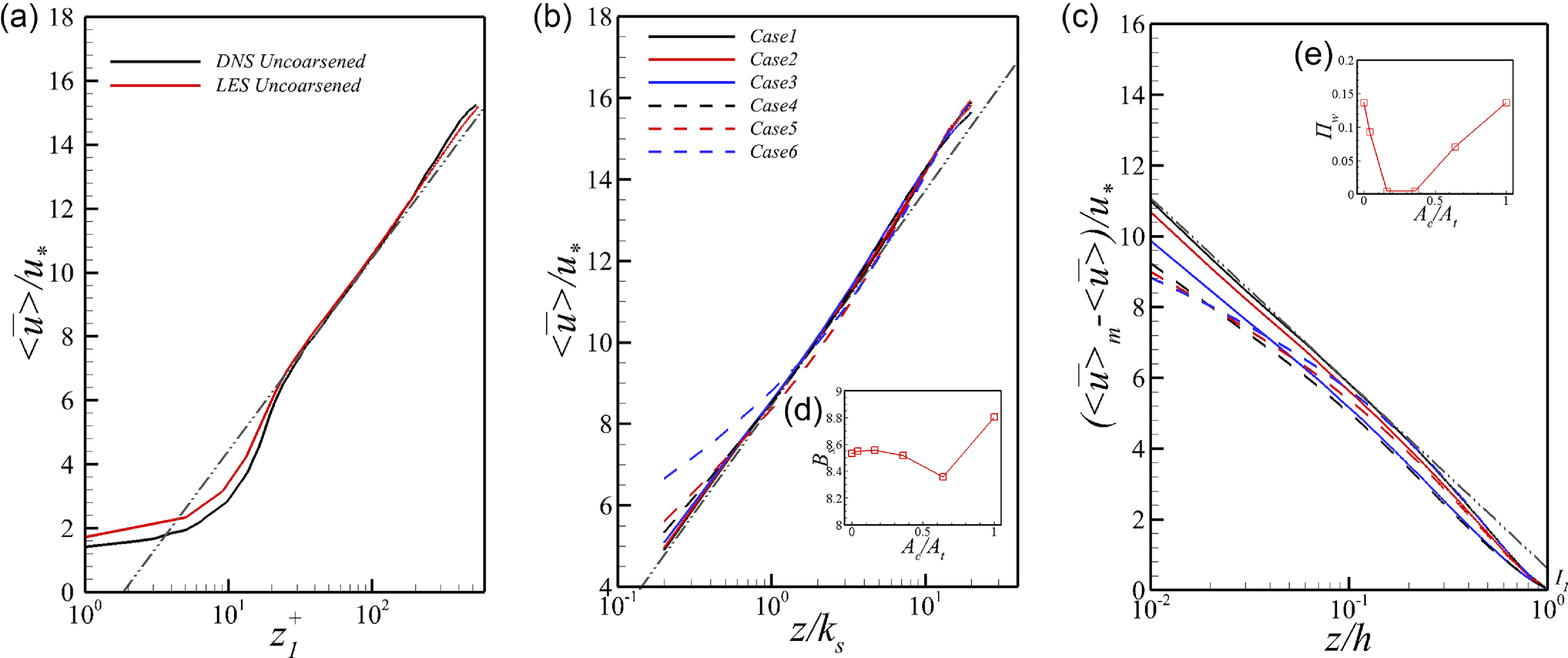
Table 2 shows that the particle Reynolds numbers for both finer and coarser spheres are significantly greater than 70, confirming that the flow is in the fully rough regime. Consequently, the velocity profiles in cases 1 to 6 are analysed as functions of distance normalised by two outer-scaled heights: z/k s (Figure 2b) and z/h (Figure 2c). In Figure 2(b), Eq. (1) is included as a dash-dotted line for reference, where $\kappa =0.43$
determined by best-fitting the lower portion of the velocity profile in case 1 to this reference line. Given
$\kappa =0.43$
determined by best-fitting the lower portion of the velocity profile in case 1 to this reference line. Given $B_{s}=8.5$
, the roughness height in Equation (1) can be explicitly determined for case 1 as
$B_{s}=8.5$
, the roughness height in Equation (1) can be explicitly determined for case 1 as $k_{s}=0.2d$
. This value is comparable in magnitude to the previously mentioned distance from the roughness top to the virtual channel bed (0.15d, as determined in Mazzuoli and Uhlmann Reference Mazzuoli and Uhlmann2017), although it is significantly lower than the roughness height range suggested in prior studies (e.g.
$k_{s}=0.2d$
. This value is comparable in magnitude to the previously mentioned distance from the roughness top to the virtual channel bed (0.15d, as determined in Mazzuoli and Uhlmann Reference Mazzuoli and Uhlmann2017), although it is significantly lower than the roughness height range suggested in prior studies (e.g. $k_{s}=2d$
in Da Silva and Yalin Reference Da Silva and Yalin2017 and
$k_{s}=2d$
in Da Silva and Yalin Reference Da Silva and Yalin2017 and $k_{s}=3d$
in Van Rijn Reference Van Rijn1984b). This discrepancy is attributed to the cubic-packing configuration of the bed spheres. By applying the roughness height of
$k_{s}=3d$
in Van Rijn Reference Van Rijn1984b). This discrepancy is attributed to the cubic-packing configuration of the bed spheres. By applying the roughness height of $0.2d$
to cases 2 to 6, the variation in
$0.2d$
to cases 2 to 6, the variation in $B_{s}$
reveals the impact of roughness effects in the mean flow. Figure 2(b) shows that, in cases 1 to 3,
$B_{s}$
reveals the impact of roughness effects in the mean flow. Figure 2(b) shows that, in cases 1 to 3, $\lt \overline{u}\gt /u_{\mathrm{*}}$
increases linearly within
$\lt \overline{u}\gt /u_{\mathrm{*}}$
increases linearly within $z/k_{s}\lt 1$
, whereas in cases 4 to 6, the roughness sublayer effect is evident in the same region. The roughness coefficient for each case, defined as
$z/k_{s}\lt 1$
, whereas in cases 4 to 6, the roughness sublayer effect is evident in the same region. The roughness coefficient for each case, defined as $B_{s}=\left.\lt \overline{u}\gt /u_{*}\right| _{z=0}$
, is presented in Figure 2d. It exhibits a slight decreasing trend up to A c/A t = 64 %, followed by an increase in the fully coarsened scenario. However, the variation in
$B_{s}=\left.\lt \overline{u}\gt /u_{*}\right| _{z=0}$
, is presented in Figure 2d. It exhibits a slight decreasing trend up to A c/A t = 64 %, followed by an increase in the fully coarsened scenario. However, the variation in $B_{s}$
remains within 4 %, indicating that increasing the coverage ratio has an insignificant impact on roughness effects in the mean flow.
$B_{s}$
remains within 4 %, indicating that increasing the coverage ratio has an insignificant impact on roughness effects in the mean flow.
Mesh resolution and domain details
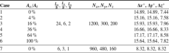
Figure 2(b) also reveals that the wake effects becomes prominent for all cases at $z/k_{s}\gt 7$
, causing deviations from the logarithmic law. To quantify this impact, defect velocity profiles as a function of the relative depth (z/h) are plotted in Figure 2(c). In this figure, the defect law is represented by a dash-dotted line, given by
$z/k_{s}\gt 7$
, causing deviations from the logarithmic law. To quantify this impact, defect velocity profiles as a function of the relative depth (z/h) are plotted in Figure 2(c). In this figure, the defect law is represented by a dash-dotted line, given by
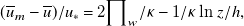 \begin{equation}(\overline{u}_{m}-\overline{u})/u_{*}=2{\prod} _{w}/\kappa -1/\kappa \ln z/h,\end{equation}
where $\kappa =0.43$
,
$\kappa =0.43$
, $\overline{u}_{m}$
is the maximum velocity at z = h and
$\overline{u}_{m}$
is the maximum velocity at z = h and ${\prod} _{w}=0.136$
is the wake strength coefficient, determined from the y-axis intercept (
${\prod} _{w}=0.136$
is the wake strength coefficient, determined from the y-axis intercept ( $I_{1})$
in case 1 using
$I_{1})$
in case 1 using ${\prod} _{w}=0.5\kappa \mathrm{I}_{1}$
. Notably, adjusting the y-axis intercept shifts the dash-dotted line parallelly upward or downward. The wake strength coefficients
${\prod} _{w}=0.5\kappa \mathrm{I}_{1}$
. Notably, adjusting the y-axis intercept shifts the dash-dotted line parallelly upward or downward. The wake strength coefficients $({\prod} _{w}$
) for cases 1 to 3 are determined by best fitting the velocity profiles within z/h<0.1. For cases 4 to 6, they are set based on the upper boundary of each velocity profile, assuming that deviations from the defect law in the lower portion result from roughness sublayer effects. For the uncoarsened case, the wake strength coefficient (
$({\prod} _{w}$
) for cases 1 to 3 are determined by best fitting the velocity profiles within z/h<0.1. For cases 4 to 6, they are set based on the upper boundary of each velocity profile, assuming that deviations from the defect law in the lower portion result from roughness sublayer effects. For the uncoarsened case, the wake strength coefficient ( ${\prod} _{w}=0.136)$
is slightly lower than that reported for smooth rectangular open-channel flow (
${\prod} _{w}=0.136)$
is slightly lower than that reported for smooth rectangular open-channel flow ( ${\prod} _{w}\approx 0.2$
in Guo Reference Guo2014), likely due to the roughness effect. As the coverage ratio increase, particularly at A c/A t = 16 % and A c/A t = 36 %,
${\prod} _{w}\approx 0.2$
in Guo Reference Guo2014), likely due to the roughness effect. As the coverage ratio increase, particularly at A c/A t = 16 % and A c/A t = 36 %, ${\prod} _{w}$
approaches zero, indicating the absence of a wake region. This is attributed to significant SCs that disrupt wake formation, which is discussed later in Figure 4. In the fully coarsened case, the wake region re-emerges, with a wake strength coefficient nearly identical to that of the uncoarsened case.
${\prod} _{w}$
approaches zero, indicating the absence of a wake region. This is attributed to significant SCs that disrupt wake formation, which is discussed later in Figure 4. In the fully coarsened case, the wake region re-emerges, with a wake strength coefficient nearly identical to that of the uncoarsened case.
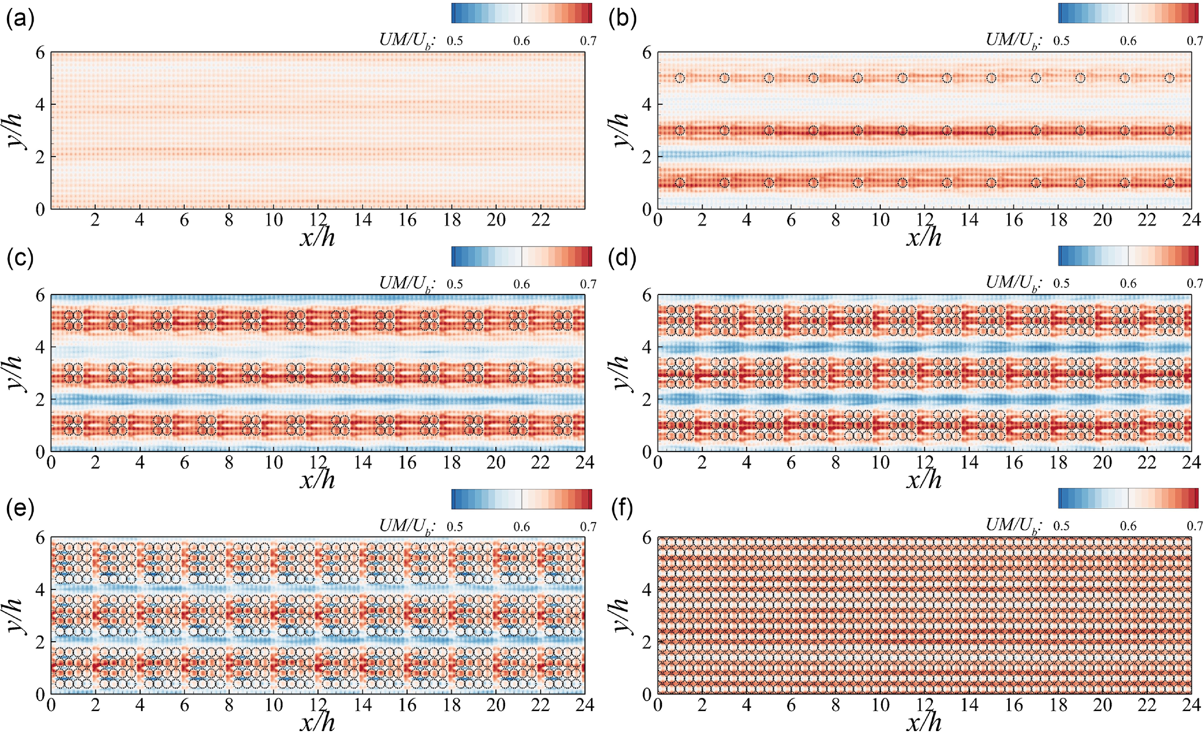
Contours of the time-averaged streamwise velocity, normalised by the bulk flow velocity, at the horizontal plane z/h = 0.04 (z = 0.002m) for case 1(a) to case 6(f).
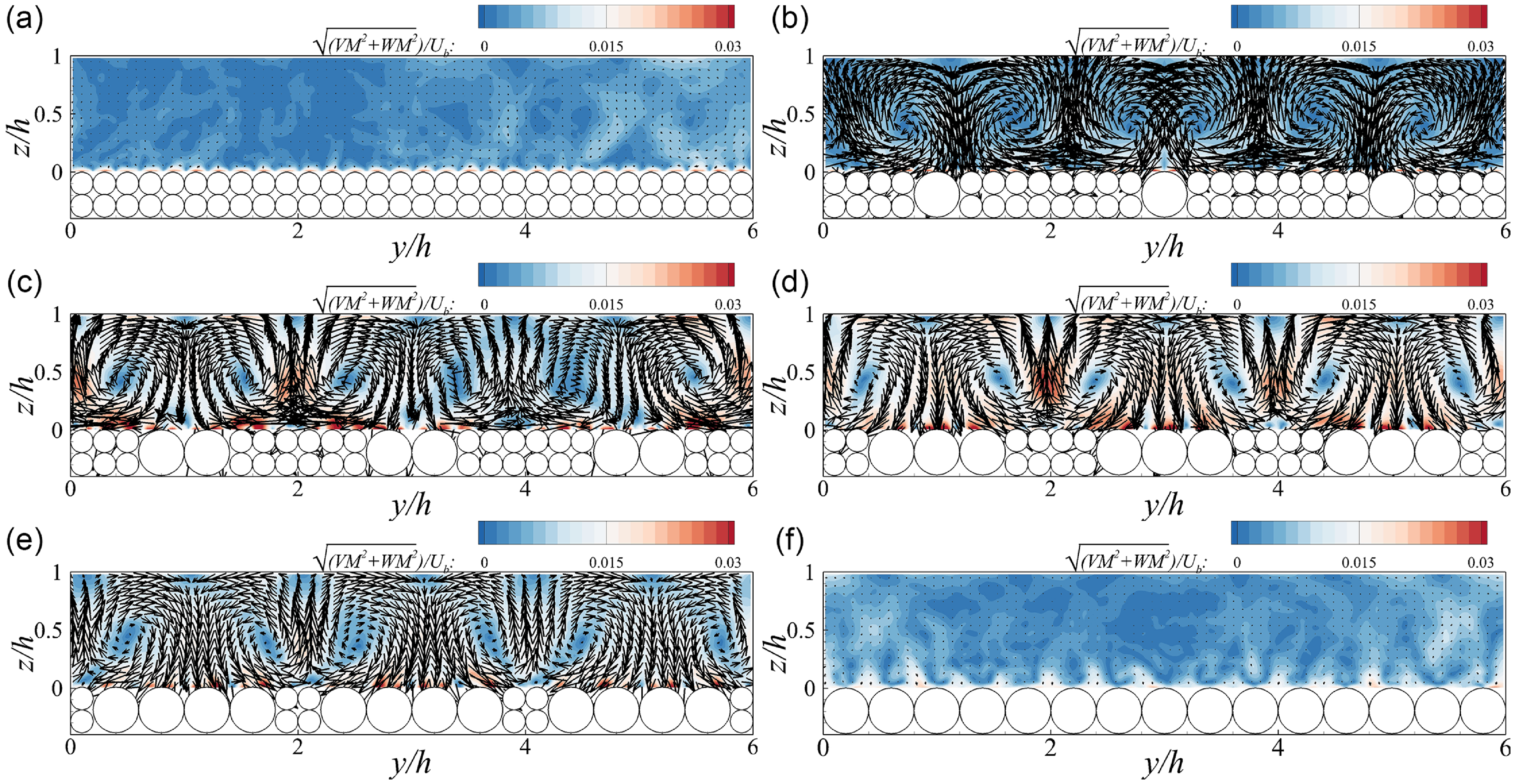
Contours of the normalised time-averaged SCs along with the in-plane velocity vector ( $\overline{v},\overline{w}$
) at the cross-section for case 1 (a) to case 6(f).
$\overline{v},\overline{w}$
) at the cross-section for case 1 (a) to case 6(f).
3.2. Time-averaged velocities and hyporheic exchange
Figure 3 presents the contours of the time-averaged streamwise velocity at the horizontal plane z/h = 0.04 for all studied cases without case 7. In the uncoarsened case, the normalised time-averaged streamwise velocity remains between 0.57 and 0.63, with weak low- and high-velocity streaks observed across the spanwise direction. These weak streaks are likely caused by the effect of the streamwise periodic boundary condition with a limited domain length. In contrast, partially coarsened cases (Figures 3b to 3e) display apparent alternating low- and high-velocity streaks spanning the domain length in the spanwise direction. The normalised time-averaged streamwise velocities for low- and high-speed streaks in these cases are approximately 0.52 and 0.72, respectively, showing limited fluctuation as the coverage ratio increases. The low-velocity streaks are predominantly positioned above regions with finer spheres, while high-velocity streaks extend over areas containing coarser particles. Spatially, the width of high-velocity streaks increases consistently as the width of area containing coarser particles expands. It is noteworthy that in these high-velocity regions, narrow low-speed strips become localised in the interspace upstream of coarser spheres, particularly visible in Figures 3(c) and 3(d). In the fully coarsened case with a coverage ratio of 100 %, both the low- and high-velocity streaks and the localised low-speed strips disappear, producing a streamwise velocity distribution that resembles the uncoarsened case but with a slightly higher average magnitude of approximately 0.68.
Figure 4(a)-(f) demonstrates the presence of the SCs revealed with the time-averaged velocity vectors in the cross-sectional planes located above particle centres. In the uncoarsened case, secondary currents are minimal, with no fully developed circulation patterns or significant peak values observed. In contrast, the partially coarsened cases (Figures 4b to 4e) display three pairs of secondary vortices along the spanwise direction, characterised by downwelling and upwelling flows well above the coarser and finer particles, respectively. The downwelling flow transports high-momentum fluid toward the roughness top, while the upwelling flow has the opposite effect, contributing the low- and high-velocity streaks observed in Figures 3(b) to Figure 3(e). The peak values of SCs reach as high as 0.028 bulk velocity above the coarser spheres. The sizes of these SCs equal to the water depth and the vortex cores are located around z/h = 0.5 across all four partially coarsened cases. In the fully coarsened case, there is no evident peak in SCs in the cross-section, nor are there significant circulation patterns. Overall, SCs strengthen with increasing coverage ratio of coarser particles in partially coarsened cases, while both the uncoarsened and fully coarsened cases exhibit negligible SCs. This is further supported by the contours of streamwise time-averaged vorticity shown in Figure S1 in the supplement, where the vorticity magnitude initially increases with increasing coverage ratio of coarser particles and followed by a decrease when A c/A t exceeds 60 %.
In order to figure out the origin of the narrow low-speed stripes in partially coarsened cases, contours of the streamwise velocity near the roughness top at the void plane and the core plane are presented in Figure 5 and Fig. S2 in the supplement, respectively, along with the time-averaged in-plane streamlines.
Contours of the normalised time-averaged streamwise velocity along with in-plane streamlines at the void plane for case 1(a) to case 6(f).
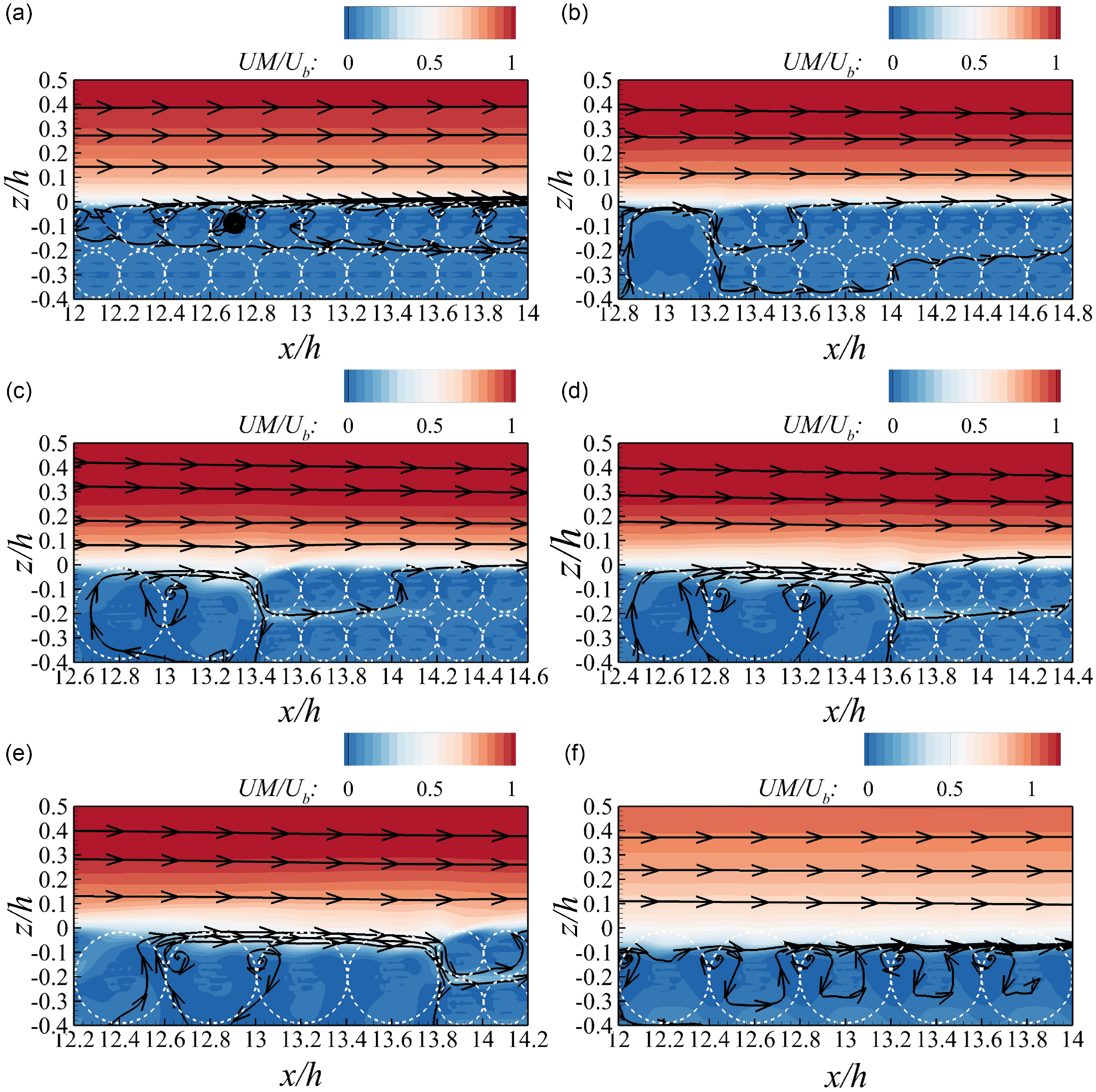
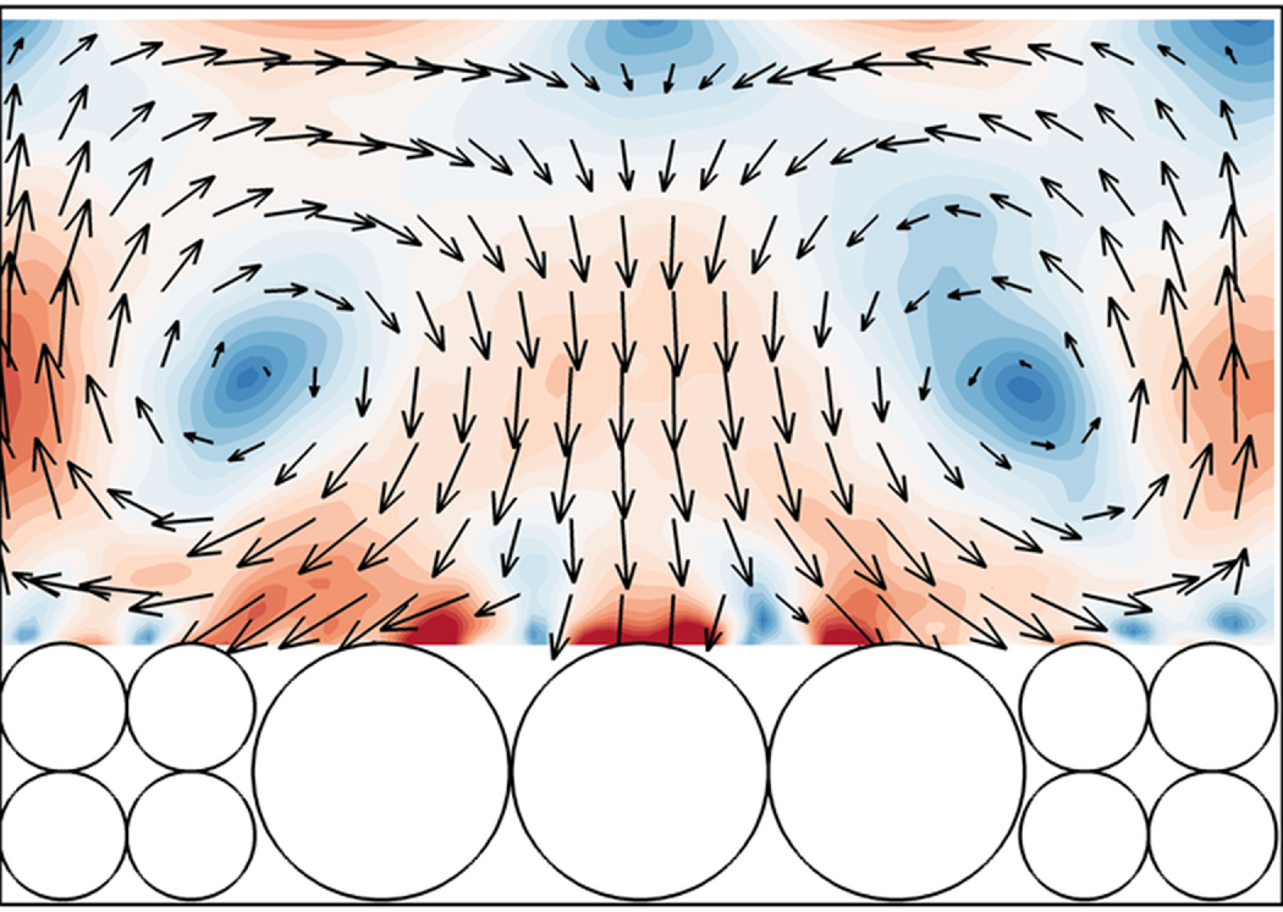
In the uncoarsened case (Figure 5a), localised flow recirculation is observed in the interspace between adjacent bed spheres near the roughness top. This recirculation extends downward to the elevation of the centres of the top-layer spheres, indicating no flow exchange between the surface flow and the subsurface flow underneath the top layer. When coarser spheres are introduced, downwelling flow intensifies at the downstream edge of the coarser spheres. This downwelling flow penetrates to a depth below the second layer of finer spheres, returning to the surface through the interspaces between the finer spheres. As a consequence, high-momentum fluid is transported toward the roughness top in the downwelling region and injected into the subsurface pores. This effect is particularly evident in Figures 5c to 5e, where an interstitial flow of velocity up to 0.5U b is observed in the pores between the top and second layers of finer spheres immediately downstream of the coarser spheres. Meanwhile, upwelling flow through the interspaces between finer spheres brings low-momentum subsurface fluid to the overlying flow, reducing near-bed flow velocity and accounting for the localised low-speed strips seen in Figures 3c to 3e. In the interspace between two adjacent coarser spheres, clockwise-rotating vortices form. In the partially coarsened cases, these vortices facilitate hyporheic exchange, reaching depths below z/h = −0.4 (Figures 5c to 5e), whereas in the fully coarsened case (Figure 5f), the vortex penetration depth is limited to within 0.3h. Figure S2 depicts the contours of time-averaged streamwise velocity and the streamlines at the core plane for all cases. Overall, an apparent hyporheic exchange is observed across all cases, due to blockage by the bed substrates. Small vortices appear near the roughness top in each case, with larger vortices forming in the interstitial spaces between coarser spheres.
3.3. Reynolds shear stress
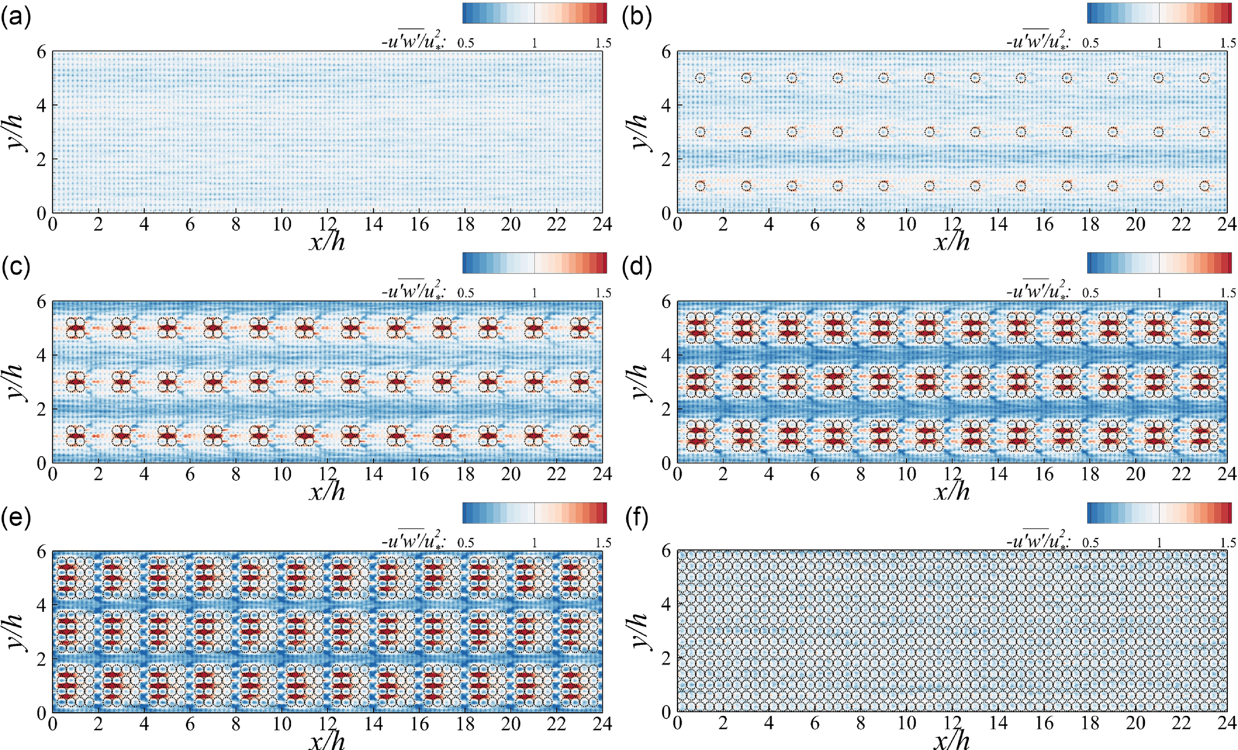
The normalised Reynolds shear stress ( $-\overline{u\mathrm{'}w\mathrm{'}}/u_{*}^{2}$
) at the horizontal plane z/h = 0.04 is shown in Figure 6. In both the uncoarsened (Figure 6a) and fully coarsened (Figure 6f) cases, the Reynolds shear stress at z/h = 0.04 remains relatively constant at
$-\overline{u\mathrm{'}w\mathrm{'}}/u_{*}^{2}$
) at the horizontal plane z/h = 0.04 is shown in Figure 6. In both the uncoarsened (Figure 6a) and fully coarsened (Figure 6f) cases, the Reynolds shear stress at z/h = 0.04 remains relatively constant at $-\overline{u'w'}/u_{*}^{2}\approx 0.9$
. In the partially coarsened cases (Figures 6b to 6e), the Reynolds shear stress distribution follows a pattern similar to the near-bed streamwise velocity distribution observed in Figures 3b to 3e. Low- and high-stress streaks, spanning the entire domain length, emerge above finer and coarser particles, respectively, corresponding to streaks of lower and higher flow velocity. These alternating streaks are influenced by the time-averaged secondary flow, which intensifies
$-\overline{u'w'}/u_{*}^{2}\approx 0.9$
. In the partially coarsened cases (Figures 6b to 6e), the Reynolds shear stress distribution follows a pattern similar to the near-bed streamwise velocity distribution observed in Figures 3b to 3e. Low- and high-stress streaks, spanning the entire domain length, emerge above finer and coarser particles, respectively, corresponding to streaks of lower and higher flow velocity. These alternating streaks are influenced by the time-averaged secondary flow, which intensifies $-\overline{u'w'}/u_{*}^{2}$
in regions of downwelling flow and reduces it in regions of upwelling flow (Figure 4). This interrelationship aligns with findings in open-channel flow over non-uniformly roughened beds (Stoesser et al. Reference Stoesser, McSherry and Fraga2015) and partially filled pipes (Liu et al. Reference Liu, Wang, Yang, Fan, Wu, Hu and Bi2022). Within the high-stress streak, the Reynolds shear stress attains the maximum value at both sides of coarser spheres in the interstitial space. The Reynolds shear stress peaks at
$-\overline{u'w'}/u_{*}^{2}$
in regions of downwelling flow and reduces it in regions of upwelling flow (Figure 4). This interrelationship aligns with findings in open-channel flow over non-uniformly roughened beds (Stoesser et al. Reference Stoesser, McSherry and Fraga2015) and partially filled pipes (Liu et al. Reference Liu, Wang, Yang, Fan, Wu, Hu and Bi2022). Within the high-stress streak, the Reynolds shear stress attains the maximum value at both sides of coarser spheres in the interstitial space. The Reynolds shear stress peaks at $-\overline{u'w'}/u_{*}^{2}$
= 1.9, indicating a dominant contribution to the spatially averaged bed shear stress. In order to further illustrate the origin of this localised Reynolds shear stress maxima in the interstitial space, the distribution of
$-\overline{u'w'}/u_{*}^{2}$
= 1.9, indicating a dominant contribution to the spatially averaged bed shear stress. In order to further illustrate the origin of this localised Reynolds shear stress maxima in the interstitial space, the distribution of $-\overline{u'w'}/u_{*}^{2}$
at both the void and core planes for all cases is separately presented in Figures 7 and 8.
$-\overline{u'w'}/u_{*}^{2}$
at both the void and core planes for all cases is separately presented in Figures 7 and 8.
Distribution of the Reynolds shear stress ( $-\overline{u\mathrm{'}w\mathrm{'}}/u_{*}^{2}$
) at the horizontal plane z/h = 0.04 for case 1(a) to case 6(f).
$-\overline{u\mathrm{'}w\mathrm{'}}/u_{*}^{2}$
) at the horizontal plane z/h = 0.04 for case 1(a) to case 6(f).
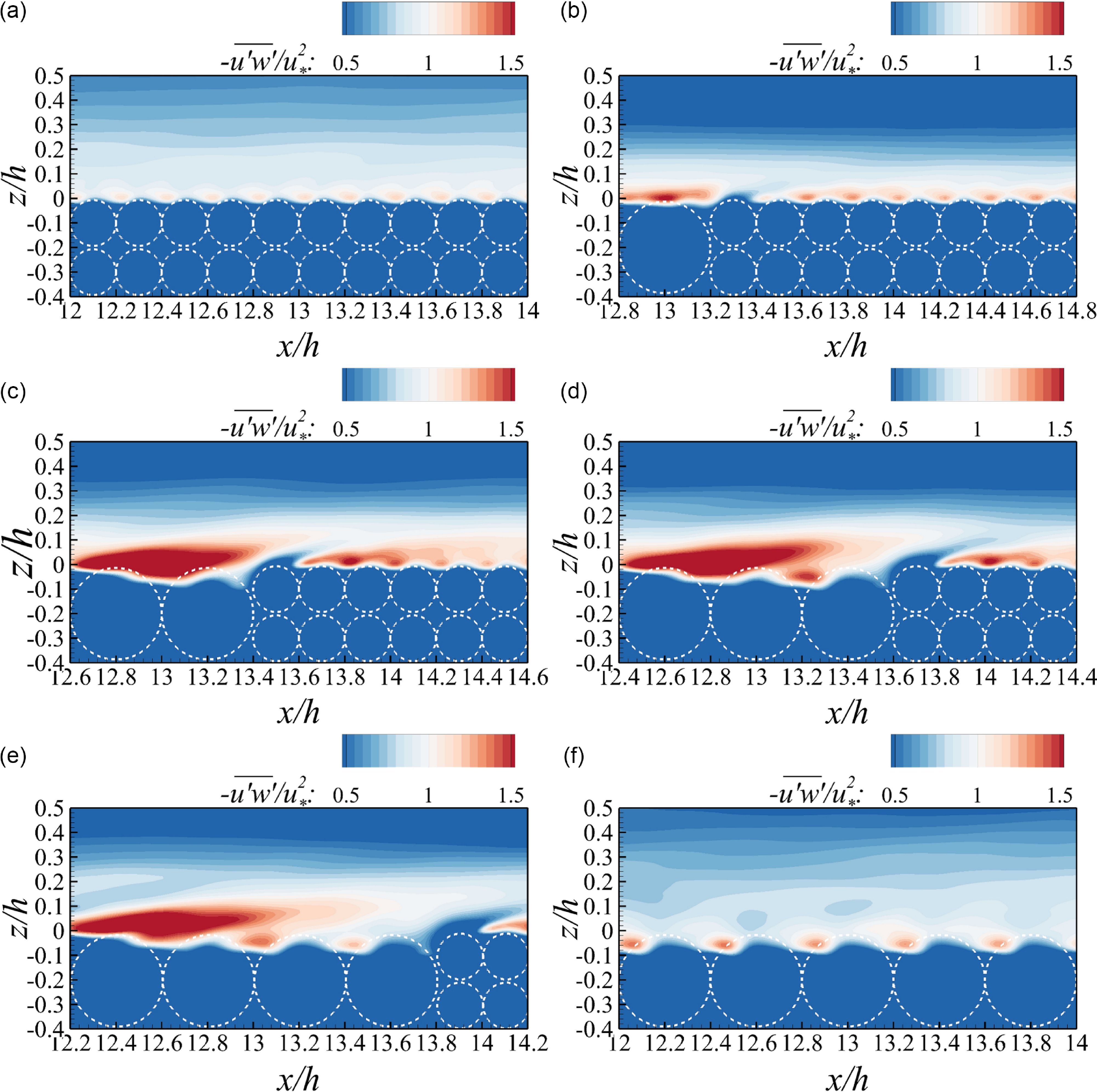
Contours of the Reynolds shear stress ( $-\overline{u'w'}/u_{*}^{2}$
) at the void plane for case 1(a) to case 6(f).
$-\overline{u'w'}/u_{*}^{2}$
) at the void plane for case 1(a) to case 6(f).
Contours of the Reynolds shear stress ( $-\overline{u'w'}/u_{*}^{2}$
) at the core plane for case 1 (a) to case 6 (f).
$-\overline{u'w'}/u_{*}^{2}$
) at the core plane for case 1 (a) to case 6 (f).
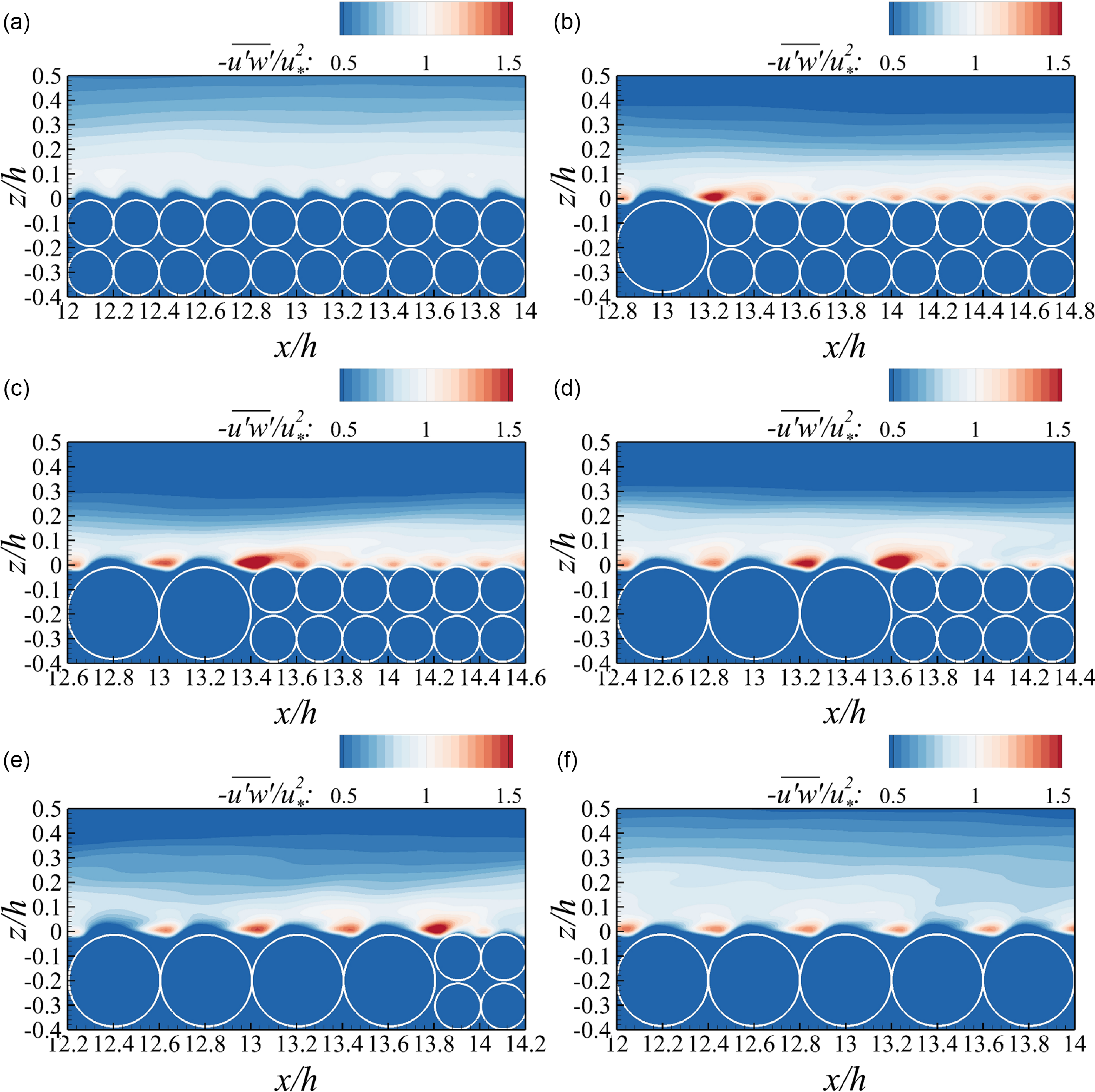
In the uncoarsened case, the Reynolds shear stress remains relatively uniform at the same elevation, with a slight increase observed upstream of each bed sphere. In the partially coarsened cases, however, an elongated high-stress layer emerges within the range −0.1 < z/h<0.1 from the upstream edge of coarser particles. This high-stress layer extends a length of D in case 2 and becomes more pronounced in cases 3 to 5, as its shape and size are similar in these three cases. Above the first finer sphere downstream of the coarser particles, an arch-shape low-stress region appears, featuring an elongated tail that stretches downstream and upward. Following this, both the value and shape of the Reynolds shear stress recover to a state similar to that in the uncoarsened case. In the fully coarsened case, the Reynolds shear stress distribution resembles the uncoarsened pattern, with one exception: the high-stress regions upstream of the coarser particles are located deeper compared with those upstream of the finer spheres, owing to larger interspace vortices, as shown in Figure 5.
The impact of the coarsened riverbed on $-\overline{u'w'}/u_{*}^{2}$
at the core plane illustrating in Figure 8, is less pronounced than at the void plane. Across all cases, low-stress regions, with
$-\overline{u'w'}/u_{*}^{2}$
at the core plane illustrating in Figure 8, is less pronounced than at the void plane. Across all cases, low-stress regions, with $-\overline{u'w'}/u_{*}^{2}$
< 0.5, hump up above the crests of finer spheres in the uncoarsened case and above the crests of coarser spheres in disturbed cases. However, a small high-stress region is observed upstream of the first finer sphere in all partially coarsened cases region upstream of the first finer sphere in all partially coarsened cases. Meanwhile, no humped low-stress regions are observed above the finer spheres in these partially coarsened cases. Both phenomena are likely attributed to local small vortices, as evident in Figure S2.
$-\overline{u'w'}/u_{*}^{2}$
< 0.5, hump up above the crests of finer spheres in the uncoarsened case and above the crests of coarser spheres in disturbed cases. However, a small high-stress region is observed upstream of the first finer sphere in all partially coarsened cases region upstream of the first finer sphere in all partially coarsened cases. Meanwhile, no humped low-stress regions are observed above the finer spheres in these partially coarsened cases. Both phenomena are likely attributed to local small vortices, as evident in Figure S2.
The distributions of high-stress regions upstream of bed spheres in both the uncoarsened and fully coarsened cases align with observations in the literature (Mazzuoli & Uhlmann Reference Mazzuoli and Uhlmann2017). However, Figures 7 and 8 reveal that, in cases where the riverbed is inhomogeneous, the near-bed Reynolds shear stress is consistently enhanced, especially in the spaces between bed spheres where upwelling flow from subsurface pores intersects with the surface flow. This emphasises the role of hyporheic flow in stimulating the near-bed Reynolds shear stress, potentially leading to an increase in reach-averaged bed shear stress.
3.4. Quadrant analysis
In order to decompose the contributions of different turbulent events to the near-bed Reynolds shear stress across all cases, the quadrant analysis is applied to time serials of velocities sampled at the void and core planes at z/h = 0.04. The joint distribution of $u'$
and
$u'$
and $w'$
is divided into four quadrants: Q1-outward interactions (
$w'$
is divided into four quadrants: Q1-outward interactions ( $u'$
>0,
$u'$
>0, $w'$
>0), Q2-ejections (
$w'$
>0), Q2-ejections ( $u'$
<0,
$u'$
<0, $w'$
>0), Q3-inward interactions (
$w'$
>0), Q3-inward interactions ( $u'$
<0,
$u'$
<0, $w'$
<0) and Q4-sweeps (
$w'$
<0) and Q4-sweeps ( $u'$
>0,
$u'$
>0, $w'$
<0).
$w'$
<0).
Quadrant analysis of normalised streamwise and vertical velocity fluctuation located at z/h = 0.04 at the void plane for case 1(a) to case 6(f).

Figures 9 and S3 present the quadrant distributions of $u'$
and
$u'$
and $w'$
normalised by the bulk flow velocity at the sampling locations at the void and core planes, respectively. The hyperbolic lines of
$w'$
normalised by the bulk flow velocity at the sampling locations at the void and core planes, respectively. The hyperbolic lines of $|u'w'|=H_{0}|\overline{u'w'}|$
with
$|u'w'|=H_{0}|\overline{u'w'}|$
with $H_{0}$
= 3.5 are also shown in these figures. Instantaneous velocity fluctuations
$H_{0}$
= 3.5 are also shown in these figures. Instantaneous velocity fluctuations $(u',w')$
falling in between these hyperbolic lines indicate snapshots with low instantaneous shear stress, i.e.
$(u',w')$
falling in between these hyperbolic lines indicate snapshots with low instantaneous shear stress, i.e. $| u'w'| \lt H_{0}|\overline{u'w'}|$
, while the data points falling outside represent high instantaneous shear stresses (Brunet Reference Brunet2020; Wallace Reference Wallace2016). Subsequently, the contributions of these high shear stress events to the Reynolds shear stresses in each quadrant, Si, H0, are calculated as
$| u'w'| \lt H_{0}|\overline{u'w'}|$
, while the data points falling outside represent high instantaneous shear stresses (Brunet Reference Brunet2020; Wallace Reference Wallace2016). Subsequently, the contributions of these high shear stress events to the Reynolds shear stresses in each quadrant, Si, H0, are calculated as
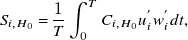 \begin{equation}S_{{i,H_{0}}}=\frac{1}{T}\int _{0}^{T}C_{{i,H_{0}}}u_{i}^{'}w_{i}^{'}dt,\end{equation}
 \begin{equation}C_{{i,H_{0}}}=\begin{cases} 1,\left| u_{i}^{'}w_{i}^{'}\right| \gt H_{0}\left| \overline{u'w'}\right| \cap \left| u_{i}^{'}w_{i}^{'}\right| \in Q_{i},\\ 0,\left| u_{i}^{'}w_{i}^{'}\right| \leq H_{0}\left| \overline{u'w'}\right| \cup \left| u_{i}^{'}w_{i}^{'}\right| \notin Q_{i}. \end{cases}\end{equation}
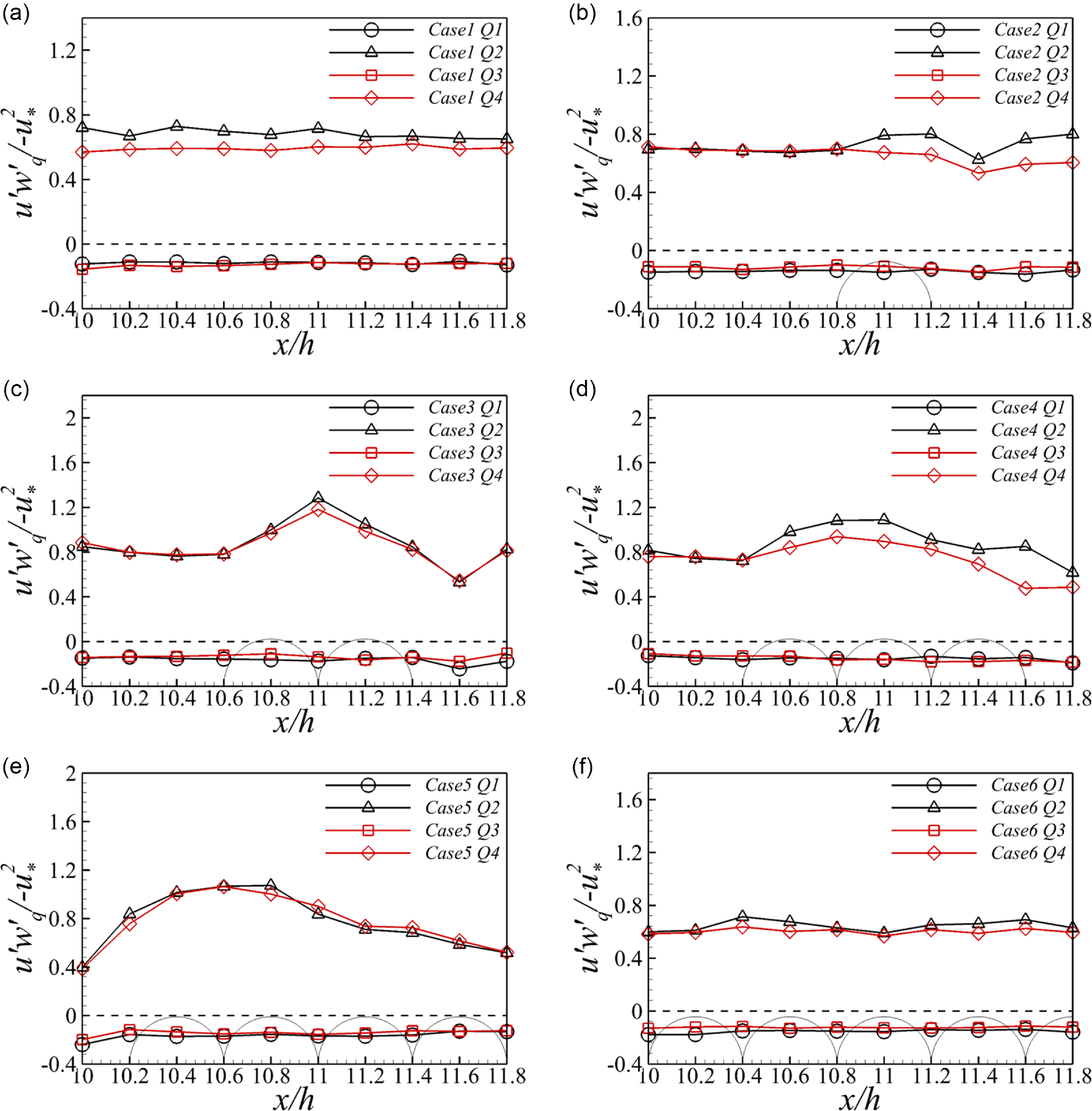
Figure 9 shows that ejections and sweeps are the dominant events across all cases at the void plane. The coverage ratio notably influences the contributions from high shear stress events. In the uncoarsened case, high shear stress ejections and sweeps contribute 6.52 % and 5.11 % to the Reynolds shear stress with prominent of ejection, respectively, while outward and inward interactions make minimal contributions of −0.28 % and −0.44 %. In the partially coarsened cases, contributions from high shear stress ejections and sweeps increase substantially, reaching up to 9.05 % and 8.57 % in case 3. When the channel bed is fully covered by coarser particles, sweeps become the most prominent events, contributing 6.09 % to Reynolds shear stress, followed by sweep at 5.16 %. The elevated Reynolds shear stress at the void plane (shown in Figure 7) can be attributed to enhanced contributions from both high shear stress ejections and sweeps. These intense turbulent events result from the interaction of subsurface and surface flows, as illustrated in Figure 5. When surface currents dominate, strong sweeps are detected, as high-velocity surface flow is directed downward at sampling points. Conversely, strong ejections occur during subsurface upwelling flow. This pattern is further confirmed in the quadrant analysis at the core plane in Figure S3. Introducing coarser particles in the partially coarsened cases triples the contribution from sweeps, while having little effect on ejections due to limited pore spaces that restrict subsurface upwelling at this plane (Figure S2).
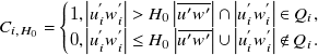
Furthermore, the spatial variation of the contribution from each quadrant, $S_{{i,H_{0}}=0}$
, along the streamwise direction is analysed in Figure 10 and in Figure S4. The contribution from each quadrant is normalised by
$S_{{i,H_{0}}=0}$
, along the streamwise direction is analysed in Figure 10 and in Figure S4. The contribution from each quadrant is normalised by $-u_{\mathrm{*}}^{2}$
, so the magnitudes in Figure 10 represent proportions relative to the reach-averaged bed stresses. At the void plane, ejections and sweeps are the two dominate events, contributing approximately 70 % and 56 %, respectively, to the reach-averaged bed shear stress, with variations within 10 % in different streamwise locations. When coarser particles are introduced, strong variations are observed along the streamwise locations. Generally, above the coarser particles, the contributions from both ejections and sweeps are significantly enhanced across all partially coarsened scenarios. Maximum contributions reach up to 130 % for ejections and 110 % for sweeps in case 3 (Figure 10c), approximately doubling their contributions in the uncoarsened case. However, downstream of the last coarser particle, these two turbulent events are suppressed, resulting in lower contributions to the reach-averaged bed stresses – up to 40 % for both events in case 5 (Figure 10e). In the fully coarsened case, the contributions from ejections and sweeps return to proportions similar to the uncoarsened case. The contributions from outward and inward interactions are minimally affected by the coverage ratio, consistently accounting for approximately −15 % of the reach-averaged bed stresses across all cases. At the core plane (Figure S4), the contributions in the uncoarsened and fully coarsened cases are similar to those at the void plane. However, contributions from the sweeps exceed those from the ejections in partially coarsened cases, particularly in the interspace between coarser particles. This again aligns with what was inferred from Figure S2, i.e. sweeps dominant where there is a clock-wise-rotating vortex.
$-u_{\mathrm{*}}^{2}$
, so the magnitudes in Figure 10 represent proportions relative to the reach-averaged bed stresses. At the void plane, ejections and sweeps are the two dominate events, contributing approximately 70 % and 56 %, respectively, to the reach-averaged bed shear stress, with variations within 10 % in different streamwise locations. When coarser particles are introduced, strong variations are observed along the streamwise locations. Generally, above the coarser particles, the contributions from both ejections and sweeps are significantly enhanced across all partially coarsened scenarios. Maximum contributions reach up to 130 % for ejections and 110 % for sweeps in case 3 (Figure 10c), approximately doubling their contributions in the uncoarsened case. However, downstream of the last coarser particle, these two turbulent events are suppressed, resulting in lower contributions to the reach-averaged bed stresses – up to 40 % for both events in case 5 (Figure 10e). In the fully coarsened case, the contributions from ejections and sweeps return to proportions similar to the uncoarsened case. The contributions from outward and inward interactions are minimally affected by the coverage ratio, consistently accounting for approximately −15 % of the reach-averaged bed stresses across all cases. At the core plane (Figure S4), the contributions in the uncoarsened and fully coarsened cases are similar to those at the void plane. However, contributions from the sweeps exceed those from the ejections in partially coarsened cases, particularly in the interspace between coarser particles. This again aligns with what was inferred from Figure S2, i.e. sweeps dominant where there is a clock-wise-rotating vortex.
Contributions from the four quadrants to the Reynolds shear stress along the streamwise direction at the void plane for case 1 (a) to case 6 (f). (The solid circles represent the locations of the coarser particles.)
3.5. Friction factor decomposition
The previous section reveals that both the depth-scale SCs and the local-scale hyporheic exchange cause an enhancement of bed shear stress. To quantify the contribution from each mechanism, the friction factor decomposition proposed by Nikora et al. (Reference Nikora, Stoesser, Cameron, Stewart, Papadopoulos, Ouro, McSherry, Zampiron, Marusic and Falconer2019) is applied as
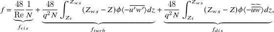 \begin{equation}f=\underset{f_{vis}}{\underbrace{\frac{48}{\mathrm{Re}}\frac{1}{N}}}+\underset{f_{turb}}{\underbrace{\frac{48}{q^{2}N}\int _{Z_{t}}^{Z_{ws}}(Z_{ws}-Z)\phi \langle -\overline{u'w'}\rangle dz}}+\underset{f_{dis}}{\underbrace{\frac{48}{q^{2}N}\int _{Z_{t}}^{Z_{ws}}(Z_{ws}-Z)\phi \langle -\widetilde{\overline{u}}\widetilde{\overline{w}}\rangle dz}} ,\end{equation}
where N is a parameter characterising flow–rough-bed interactions; q is the specific flow rate per unit width; Z ws is water depth; Z t is the roughness troughs; $\phi$
is roughness geometry function. The parameters
$\phi$
is roughness geometry function. The parameters $f_{vis}$
,
$f_{vis}$
, $f_{turb}$
,
$f_{turb}$
, $f_{dis}$
represent the contributions from viscosity, turbulent stresses and dispersive stresses, respectively. This decomposition has the advantage that it explicitly accounts for the local scale, through the ‘filtering’ effect of the spatial averaging domain (Nikora et al. Reference Nikora, Stoesser, Cameron, Stewart, Papadopoulos, Ouro, McSherry, Zampiron, Marusic and Falconer2019) and has been widely applied in turbulent boundary layers and open-channel flows (Xu et al. Reference Xu, Zhong and Zhang2020; Zampiron et al. Reference Zampiron, Cameron and Nikora2020). In the current LES,
$f_{dis}$
represent the contributions from viscosity, turbulent stresses and dispersive stresses, respectively. This decomposition has the advantage that it explicitly accounts for the local scale, through the ‘filtering’ effect of the spatial averaging domain (Nikora et al. Reference Nikora, Stoesser, Cameron, Stewart, Papadopoulos, Ouro, McSherry, Zampiron, Marusic and Falconer2019) and has been widely applied in turbulent boundary layers and open-channel flows (Xu et al. Reference Xu, Zhong and Zhang2020; Zampiron et al. Reference Zampiron, Cameron and Nikora2020). In the current LES, $f_{dis}$
is predominantly generated by SCs and
$f_{dis}$
is predominantly generated by SCs and $f_{turb}$
quantifies the comprehensive impact of turbulent shear stresses generated by coarser particles to the total friction.
$f_{turb}$
quantifies the comprehensive impact of turbulent shear stresses generated by coarser particles to the total friction.
Figure 11 presents vertical profiles of the components of dispersive shear stress (a), turbulent shear stress (b) and the total shear stress (the sum of the two shear stresses) (c) across all cases with varying coverage ratio. The dashed-dotted line in the figure represents the gravity line, indicating the theoretical distribution of Reynolds shear stress in two-dimensional open-channel flow. In Figure 11 (a), both the uncoarsened case and fully coarsened case exhibit negligible dispersive shear stress. The turbulent shear stress accounts for the majority of the total shear stress, both coincide with the gravity line until z/h $\approx$
0.05, where viscous stress raises as expected. In the partially coarsened cases, dispersive shear stress increases, peaking around z/h = 0.4, which aligns with the position of the centres of SCs. The normalised peak values of the dispersive shear stress increases from 0.03 to 0.15 with increasing the coverage ratio until
$\approx$
0.05, where viscous stress raises as expected. In the partially coarsened cases, dispersive shear stress increases, peaking around z/h = 0.4, which aligns with the position of the centres of SCs. The normalised peak values of the dispersive shear stress increases from 0.03 to 0.15 with increasing the coverage ratio until $A_{c}/A_{t}$
= 36 %, followed by a 30 % reduction at higher coverage ratio. This indicates that SCs trigger dispersive stress in these cases. For the counterpart, contributions from the turbulent shear stress decreases with increasing
$A_{c}/A_{t}$
= 36 %, followed by a 30 % reduction at higher coverage ratio. This indicates that SCs trigger dispersive stress in these cases. For the counterpart, contributions from the turbulent shear stress decreases with increasing $A_{c}/A_{t}$
to 36 % and followed by an increase at higher
$A_{c}/A_{t}$
to 36 % and followed by an increase at higher $A_{c}/A_{t}$
. Figure 11(c) shows that the total shear stress, i.e. sum of the dispersive and turbulent shear stresses, aligns with the gravity line for all cases, thereby validating the application of the friction factor decomposition.
$A_{c}/A_{t}$
. Figure 11(c) shows that the total shear stress, i.e. sum of the dispersive and turbulent shear stresses, aligns with the gravity line for all cases, thereby validating the application of the friction factor decomposition.
Vertical profiles of the dispersive shear stresses (a), the Reynolds shear stresses (b) and the total shear stresses (c) for all cases. Panel (d) presents the components of the overall friction factor as a function of the coverage ratio.
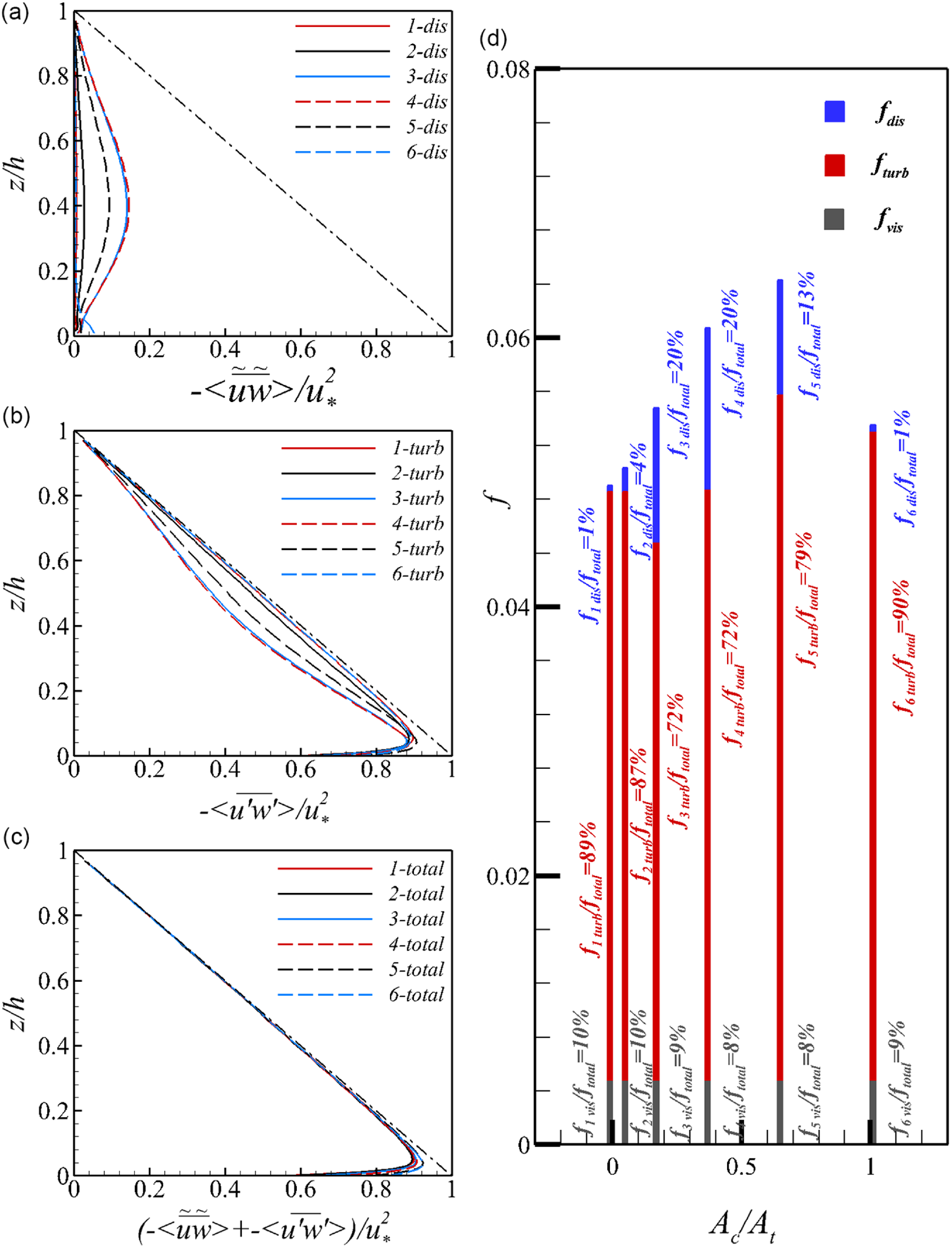
Using Eq. 7, the components of the total friction factor versus the coverage ratio are shown in Figure 11(d). Overall, the total friction factor, f, exhibits a monotonical increase up to $A_{c}/A_{t}$
= 64 %, in which its value is approximately 130 % of that in the uncoarsened case. This increase is caused by an increase in both the turbulent contribution, f turb, and the secondary flow contribution, f dis. Further coarsening the channel bed to
$A_{c}/A_{t}$
= 64 %, in which its value is approximately 130 % of that in the uncoarsened case. This increase is caused by an increase in both the turbulent contribution, f turb, and the secondary flow contribution, f dis. Further coarsening the channel bed to $A_{c}/A_{t}$
= 100 %, the total friction factor has a 15.84 % reduction, due to a significant reduction in the dispersive component. The value of the viscous component, f vis, is identical across all cases due to the identical Reynolds number applied in all simulations (Table 1), while the dispersive component, f dis, attains a maximum at
$A_{c}/A_{t}$
= 100 %, the total friction factor has a 15.84 % reduction, due to a significant reduction in the dispersive component. The value of the viscous component, f vis, is identical across all cases due to the identical Reynolds number applied in all simulations (Table 1), while the dispersive component, f dis, attains a maximum at $A_{c}/A_{t}$
= 16 %, contributing 20 % to the total friction factor. For the uncoarsened and fully coarsened cases, the turbulent component, f turb, contributes the majority (up to 88.8 %) of total friction factor.
$A_{c}/A_{t}$
= 16 %, contributing 20 % to the total friction factor. For the uncoarsened and fully coarsened cases, the turbulent component, f turb, contributes the majority (up to 88.8 %) of total friction factor.
4. Discussion
The LES results reveal that the impact of riverbed coarsening on flow resistance is governed by two primary mechanisms: (i) enhanced SCs in the outer region and (ii) intensified hyporheic exchange at the SWI.
The SCs observed in this study can be classified, at least preliminarily, as Prandtl’s second kind (Prandtl Reference Prandtl1926), driven by turbulence anisotropy. In the current LES, the maximum intensity of SCs reaches 0.028 $U_{b}$
, which is within the range reported for narrow open-channel flows (0.019
$U_{b}$
, which is within the range reported for narrow open-channel flows (0.019 $U_{b}$
−0.024
$U_{b}$
−0.024 $U_{b}$
in Kadia et al. Reference Kadia, Rüther, Albayrak and Pummer2022, and Demiral et al. Reference Demiral, Boes and Albayrak2020). However, it is lower than the intensities observed in flows over streamwise ridges ( >0.05
$U_{b}$
in Kadia et al. Reference Kadia, Rüther, Albayrak and Pummer2022, and Demiral et al. Reference Demiral, Boes and Albayrak2020). However, it is lower than the intensities observed in flows over streamwise ridges ( >0.05 $U_{b}$
in Zampiron et al. Reference Zampiron, Cameron and Nikora2020, and Luo et al. Reference Luo, Stoesser, Cameron, Nikora, Zampiron and Patella2023) and in semi-filled pipe flows (
$U_{b}$
in Zampiron et al. Reference Zampiron, Cameron and Nikora2020, and Luo et al. Reference Luo, Stoesser, Cameron, Nikora, Zampiron and Patella2023) and in semi-filled pipe flows ( $\approx$
0.05
$\approx$
0.05 $U_{b}$
in Liu et al. Reference Liu, Wang, Yang, Fan, Wu, Hu and Bi2022, and Ng et al. Reference Ng, Cregan, Dodds, Poole and Dennis2018). The SCs in the current LES span the entire flow depth, consistent with observations from flows over large-spacing streamwise ridges ( >2h; Luo et al. Reference Luo, Stoesser, Cameron, Nikora, Zampiron and Patella2023; Zampiron et al. Reference Zampiron, Cameron and Nikora2020) and flows over non-uniformly roughened channel beds (Stoesser et al. Reference Stoesser, McSherry and Fraga2015; Wangsawijaya et al. Reference Wangsawijaya, Kevin, Baidya, Monty and Hutchins2020).
$U_{b}$
in Liu et al. Reference Liu, Wang, Yang, Fan, Wu, Hu and Bi2022, and Ng et al. Reference Ng, Cregan, Dodds, Poole and Dennis2018). The SCs in the current LES span the entire flow depth, consistent with observations from flows over large-spacing streamwise ridges ( >2h; Luo et al. Reference Luo, Stoesser, Cameron, Nikora, Zampiron and Patella2023; Zampiron et al. Reference Zampiron, Cameron and Nikora2020) and flows over non-uniformly roughened channel beds (Stoesser et al. Reference Stoesser, McSherry and Fraga2015; Wangsawijaya et al. Reference Wangsawijaya, Kevin, Baidya, Monty and Hutchins2020).
The near-bed Reynolds shear stress in partially coarsened cases is significantly elevated near the coarser spheres, aligning with Stoesser et al. (Reference Stoesser, McSherry and Fraga2015), who reported that Reynolds shear stress above rough elements can reach approximately 150 % of the reach-averaged bed stress in non-uniformly roughened bed flows. Additionally, zones of maximum Reynolds shear stress, with values reaching up to 190 % of the reach-averaged bed stress, are observed in the interspaces between coarser spheres. This highlights the importance of the second mechanism – intensified hyporheic exchange.
The heterogeneity of the channel bed spheres induces localised vortices near the SWI, which enhance hyporheic exchange, particularly at the junctions of larger and finer spheres (Figure 5). Consequently, stronger vertical momentum exchange occurs in partially coarsened cases, resulting in reduced velocities above finer spheres (Figure 3) and increased velocities above coarser spheres (Figure 5). In regions with intense hyporheic exchange, the characteristics of turbulent events and their contributions to Reynolds shear stress undergo significant changes.
The introduction of coarser particles creates two types of heterogeneities: (i) surface roughness heterogeneity, which refers to variations in protrusion heights above the riverbed, and (ii) bed permeability heterogeneity. These two forms of heterogeneity typically occur together in natural riverbed coarsening processes (Parker et al. Reference Parker, An, Lamb, Garcia, Dingle and Venditti2024, Liu et al. Reference Liu, Song, Zhang, Wang, Guo, Tang, Kong and Huo2017, Zhang et al. Reference Zhang, Zhang, Tang and Zhao2017) and in flume experiments (Hill et al. Reference Hill, Gaffney, Baumgardner, Wilcock and Paola2017). While the effects of surface roughness heterogeneity have been investigated by introducing large spheres to a plane bed of small spheres (Fang et al. Reference Fang, Liu and Stoesser2017; Liu et al. Reference Liu, Tang, Huang, Stoesser and Fang2024), the impact of bed permeability heterogeneity has received a little attention. A recent direct numerical simulation has demonstrated that a riverbed consisted of random-packed uniform-sized sediment particles exhibits enhanced form-induced fluctuations and stronger vertical momentum exchange as compared with a bed with cubic-packed spheres (Shen et al. Reference Shen, Yuan and Phanikumar2020). However, the random distribution of riverbed substrates leads to both types of the aforementioned heterogeneities. In the current LES, the bed configurations allow identical crest heights for both larger and finer spheres, which isolates the effects of these two types of heterogeneities. Figures 2(b) and 2(d) illustrate that surface roughness heterogeneity has a negligible impact, as the roughness coefficient exhibits minimal variation at a constant k s. Consequently, variations in near-bed Reynolds shear stress arise solely from heterogeneous permeability. The maximum local near-bed Reynolds shear stress reaches up to 190 % of the reach-averaged bed stress, comparable to the shear stress induced by a fully protruding element (approximately twice the reach-averaged bed stress, as reported by Fang et al. Reference Fang, Liu and Stoesser2017). These results highlight the need for further investigation into more realistic coarsened riverbed conditions, including different diameter ratios of large to small spheres (Hill et al. Reference Hill, Gaffney, Baumgardner, Wilcock and Paola2017), various coarsening patterns (e.g. strip-like or random distributions), and the combined effects of both surface roughness and permeability heterogeneity.
5. Conclusion
Large-eddy simulations have been conducted to investigate the impact of riverbed coarsening on flow resistance in open-channel flow. Interestingly, the overall flow resistance reaches its maximum at an intermediate coverage ratio of coarser sediments ( $A_{c}/A_{t}$
=64 %). To uncover the underlying mechanisms behind this phenomenon, the time-averaged flow field and the distribution of Reynolds shear stresses have been analysed quantitatively. Additionally, quadrant analysis of turbulent events and the friction factor decomposition method have been employed. By comparing results across simulations with varying coverage ratios, the primary effects of riverbed coarsening are identified, leading to the following key conclusions:
$A_{c}/A_{t}$
=64 %). To uncover the underlying mechanisms behind this phenomenon, the time-averaged flow field and the distribution of Reynolds shear stresses have been analysed quantitatively. Additionally, quadrant analysis of turbulent events and the friction factor decomposition method have been employed. By comparing results across simulations with varying coverage ratios, the primary effects of riverbed coarsening are identified, leading to the following key conclusions:
(i) In partially coarsened cases, distinct low- and high-stress streaks span the entire domain length above finer and coarser particles, respectively. The highest Reynolds shear stress values are observed in the interstitial spaces between coarser spheres.
(ii) This spatial variation is attributed to two primary mechanisms: (i) enhanced SCs in the outer region, which increase the dispersive contribution to the total friction factor and (ii) intensified hyporheic exchange at the SWI, which modifies the contributions of ejections (Q2) and sweeps (Q4) to the Reynolds shear stress.
(iii) Overall, the total friction factor and the roughness coefficient at $A_{c}/A_{t}$
=64 % increase by 29.79 % and 34.93 %, respectively, compared with the uncoarsened case. These are followed by reductions of 15.84 % and 16.34 %, respectively, in the fully coarsened case (
$A_{c}/A_{t}$
=64 % increase by 29.79 % and 34.93 %, respectively, compared with the uncoarsened case. These are followed by reductions of 15.84 % and 16.34 %, respectively, in the fully coarsened case ( $A_{c}/A_{t}$
=100 %).
$A_{c}/A_{t}$
=100 %).
Supplementary data
Supplementary material and movies are available online https://doi.org/10.1017/jfm.2025.15.
Acknowledgements
We would like to acknowledge the insightful comments from both anonymous reviewers. The authors would like to acknowledge the support of the high-performance cluster centres ‘Taiyi’ of the Southern University of Science and Technology.
Funding statement
Financial support for this work was provided by the National Key Research and Development Project (No. 2022YFC3201802), the National Natural Science Foundation of China (No. 12372383), the Shenzhen Natural Science Foundation (No. JCYJ20230807093507015), and the High-level University Special Fund (No. G03050K001).
Competing interests
The authors report no conflict of interest.


 Open access