


Impact Statement
Implementing natural ventilation strategies in buildings is an efficient way of reducing their energy consumption while improving the indoor air quality. Effective ventilation can also limit the risk of transmission of airborne infection by renewing the air in the room. We develop a method to estimate the ventilation through a sash window of a room with a uniform interior temperature higher than the outdoor temperature. We show that three different flow regimes may occur and calculate the geometrical limits for the transition from one regime to another. We show that as the size of the closed panel relative to the total window area increases the ventilation rate is more sensitive to the geometry of the openings. The model developed can easily be implemented into control systems and building design.
1. Introduction
In developed countries the energy consumption used to heat and cool buildings comprises 20 % to 40 % of the total energy use (Reference Pérez-Lombard, Ortiz and PoutPérez-Lombard, Ortiz, & Pout, 2008). Compared with energy consumption in 2010, future energy cooling consumption of residential buildings worldwide is predicted to more than triple by 2050 (Reference SantamourisSantamouris, 2016), therefore strategies to reduce the cooling energy consumption of buildings are needed. Cooling can be provided by natural ventilation, which exploits buoyancy forces and wind to drive flows. Reference Chen, Tong and MalkawiChen, Tong, and Malkawi (Reference Chen, Tong and Malkawi2017), by estimating the number of suitable hours for using natural ventilation per year, demonstrated that natural ventilation can be used for at least some portion of the year in regions with climates varying from subtropical highland (Kenya, China, Mexico…) to Mediterranean (Portugal, Chile, California…). An additional reason to improve our understanding of common ventilation strategies is the strong relationship between ventilation and the transmission of airborne infections (Reference Bhagat, Davies Wykes, Dalziel and LindenBhagat, Davies Wykes, Dalziel, & Linden, 2020; Reference Bhagat and LindenBhagat & Linden, 2020; Reference Li, Leung, Tang, Yang, Chao, Lin and YuenLi et al., 2007). Effective ventilation is an important tool in our fight against infectious diseases and in maintaining good indoor air quality and thermal comfort. Implementing any ventilation strategy requires a good understanding of the flow physics along with simple and accurate models that can easily be implemented into building design and control systems.
Counter-balanced vertically sliding windows, also called sash windows, appeared at the end of the seventeenth century in England (Reference RamseyRamsey, 2009) and despite their ubiquity their inventor remains anonymous (Reference LouwLouw, 1983). At that time, improvements in glass manufacturing and new architectural legislation facilitated the development of large windows with vertical sliding panes (Reference RamseyRamsey, 2009) and consequently sash windows are currently used in many buildings and houses in northern Europe.
As illustrated in figure 1, a traditional sash window has two vertical sliding panes that allow the window to be open at the top and/or bottom. Since each pane occupies half the window area  $A$, the maximum total openable area is $A/2$. Here, we consider the flow through such a window when it is the only ventilation opening in the space. If only the top or bottom pane is open, any ventilation must occur via a two-way flow through that opening due to conservation of volume in the room. On the other hand, if both the top and bottom panes are open it is possible for air to flow in through one opening and out through the other.
Sash windows: (a) a photo of a sash window, and (b) a sketch of the geometry, which has openable window height  $H$, window width $W$, upper opening height $h_u$, lower opening height $h_l$ and closed window height $h_w$.

The natural ventilation of buildings has been widely studied in recent decades (Reference EtheridgeEtheridge, 2015; Reference Ohba and LunOhba & Lun, 2010). Research on natural ventilation through windows has focused on buoyancy-driven flow for various opening sizes, shapes and room configurations (Reference Gladstone and WoodsGladstone & Woods, 2001; Reference Grabe, Svoboda and BäumlerGrabe, Svoboda, & Bäumler, 2014; Reference Jiang and ChenJiang & Chen, 2003; Reference Li, Delsante and SymonsLi, Delsante, & Symons, 2000) and the interaction between wind and temperature (Reference Carey and EtheridgeCarey & Etheridge, 1999; Reference Davies Wykes, Chahour and LindenDavies Wykes, Chahour, & Linden, 2020; Reference Li, Delsante and SymonsLi et al., 2000; Reference Lishman and WoodsLishman & Woods, 2009).
Various full-scale experiments have been conducted on buoyancy-driven flow through sash windows. Their thermal performance and the impact of secondary glazing and window covering have been examined by Reference Wood, Bordass and BakerWood, Bordass, and Baker (Reference Wood, Bordass and Baker2009) and Reference Fitton, Swan, Hughes and BenjaberFitton, Swan, Hughes, and Benjaber (Reference Fitton, Swan, Hughes and Benjaber2017). Reference Conceiça and LúcioConceiça and Lúcio (Reference Conceiça and Lúcio2006) evaluated the efficiency of different ventilation strategies for full-scale rooms, observing that rooms with a large number of sash windows showed a higher air exchange rate. Reference Grabe, Svoboda and BäumlerGrabe et al. (Reference Grabe, Svoboda and Bäumler2014) studied ventilation efficiency through full-scale experiments, using CO $_2$ decay to measure the ventilation rate of a room for different types of windows, including a sash window. Their measurements showed that a sash window has at least a $50\,\%$ larger ventilation efficiency, in terms of mass flow, than a tilt window. In addition, among the studied windows the sash window yielded the second best ventilation performance, after the horizontal pivot window.
By performing numerical simulations on different types of windows (sash window, tilt window, vertical pivot window, etc.), Reference Wang, Wang, Zhang and BattagliaWang, Wang, Zhang, and Battaglia (Reference Wang, Wang, Zhang and Battaglia2017) showed that sash windows provide the best ventilation rates of all studied window types and the air in the ventilated room is well mixed. Using their previous results, Reference Wang, Zhang, Wang and BattagliaWang, Zhang, Wang, and Battaglia (Reference Wang, Zhang, Wang and Battaglia2017) investigated numerically gaseous pollutant cross-transmission in a three-story sash window building. The effect of changing the height of the closed panel on the ventilation performance for restricting pollutant cross-transmission to rooms above the source room was studied. The sash window and the horizontal pivot window provided the largest ventilation rates. Reference Wang, Zhang, Wang and BattagliaWang, Zhang, Wang, and Battaglia (Reference Wang, Zhang, Wang and Battaglia2018) emphasised, for single-sided natural ventilation, the impact of ambient wind on the air change rate. Their numerical simulations showed that for a sash window the temperature distribution inside the building does not change with increasing wind speed, unlike vertical or horizontal pivoting windows.
Reference Phillips and WoodsPhillips and Woods (Reference Phillips and Woods2004) developed a model for flow through doorways, which they later applied to two openings with some vertical spacing. Their steady-state model included a source of buoyancy. They observed that two openings vertically far apart provide a better ventilation rate than one opening of the same total area. In all of these research works, the height of the upper and lower openings were kept equal and only the height of the closed panel was changed. Thus no asymmetric geometry has been examined.
In this paper we examine buoyancy-driven ventilation of a closed room with an open sash window. We develop a model for the flow in § 2, demonstrating the existence of three flow regimes in § 2.1. Switching between these regimes occurs at a critical lower opening height and we extend our model for the case of a heat source in the room in § 2.2. We present an analytic model for this critical height as a function of opening area in § 2.3. We describe the set-up of our laboratory experiments in § 3 and compare our models with the results in § 4. Our conclusions are presented in § 5. We find that the arrangement of the sash window and thus the flow regime has a significant influence on the ventilation rate.
2. Theory
The key purposes of ventilation are the removal of pollutants and heat. Heat is generated indoors by occupants (body heat) and appliances, and buoyancy-driven natural ventilation utilises this heat to drive a flow and ventilate a building. During the winter, maintaining thermal comfort requires heating, and adequate ventilation is required for breathing and removal of pollutants. However, during the summer, buildings can heat significantly as a result of these internal heat sources and solar gains and ventilation is required primarily to maintain thermal comfort. This gives rise to two scenarios: firstly, wintertime ventilation where the dominant heat sources are heating devices (e.g. radiators) and the heating rate can be increased or decreased to maintain thermal comfort, i.e. indoor temperatures remain constant; secondly, summertime ventilation where the dominant heat sources are solar gains, occupants and appliances, i.e. the indoor heat supply remains relatively constant.
The sash window geometry that we consider is shown in figure 1(b). The total height of the window is  $H$ and the width of the window is $W$. The heights of the upper and lower openings are denoted respectively by $h_u$ and $h_l$, while the closed glass section height is $h_w$. We can describe the geometry of the openings using two dimensionless parameters $\alpha = {h_w}/{H}$ and $\beta = {h_l}/{H}$. The non-dimensional height of the upper opening is $1-\alpha -\beta$, while the total height of both openings is $1 - \alpha$. Note that since the height of the closed glass section is never less than half the window height, ${\textstyle \frac {1}{2}} \leq \alpha \leq 1$. As depicted in figure 2 the non-dimensional vertical coordinate is denoted by $\hat {z} = z /H$.
Schematic of the pressure gradients (left) and the velocity profile (right) at the sash window. The pressure gradient for inside (red) and outside (blue) a warm room are shown ( $T_i > T_e$). The neutral level is denoted by $\hat {z}_{n}$. The case shown has a larger upper opening ( $1-\alpha > 2\beta$), therefore the neutral level is located above the mid-height of the window $\hat {z} = 1/2$.

In the present study we focus our attention on room-to-outside ventilation and do not consider any room-to-room ventilation, which could shift the position of the neutral pressure level by increasing or decreasing the pressure in the room. We assume that the air inside the room is well-mixed and has a uniform interior temperature  $T_i$, while the exterior temperature is $T_e$ ( $T_i > T_e$), leading to a uniform density $\rho _i$ inside the room and $\rho _e$ outside ( $\rho _i < \rho _e$). The assumption that the room is well mixed will be reasonable if the heat source inside the room keeping it at steady state can be modelled as an area heat source. If we assume that away from the window the air is at rest, then in the room and in the external environment the pressure can be assumed to be hydrostatic,
 \begin{equation} \frac{\mathrm{d} p_j}{\mathrm{d} z} = {-}g\rho_j, \end{equation}
where  $g$ is the acceleration due to gravity and $j$ refers to the interior or exterior density and pressure. Under our assumptions (2.1) implies that the vertical pressure gradient is larger inside the room. There will be a height called the neutral pressure level, $z_{n}$, at which the internal and external pressures are equal. The dimensionless height of the neutral level is denoted by $\hat {z}_n$ (figure 2). In the case considered here where the indoor air is warmer than outdoors, above the neutral level the pressure difference between the room and the exterior will tend to drive flow from inside to outside, while below the neutral level, the pressure difference drives flow into the room.
From figure 2 it is clear that we are only concerned with the differences in pressure across the openings and that the pressure variations above and below the window are irrelevant. Consequently, to determine the flow through the window, we need only to consider the vertical section of the room of height  $H$ spanned by the window and ignore any stratification above or below this section.
Assuming (2.1) applies inside and outside the room, we can apply Bernoulli's principle along horizontal streamlines at the window above and below the neutral level,  $\hat {z}_n$, giving the velocity of the flow travelling from the inside to the outside, and vice versa. The Boussinesq approximation is made, that the density difference is small compared with the mean density i.e. ( $\rho _e-\rho _i \ll (\rho _e+\rho _i)/2$). The use of the Boussinesq approximation is valid since in the case of buoyancy-driven ventilation through a window we have $\Delta T \ll T$ (e.g. $\Delta T \approx 10$ K and $T \approx 300$ K). If the outdoors is warmer then the Boussinesq approximation means that the flow simply reverses direction. Furthermore, we assume that no mixing occurs between the flows at the opening. Under these assumptions, the magnitude of the flow velocity through the openings is
 \begin{equation} v(\hat{z}) = \begin{cases} (2 g' H ( \hat{z} - \hat{z}_n ))^{1/2} & \hat{z} > \hat{z}_n, \\ (2 g' H ( \hat{z}_n - \hat{z} ))^{1/2} & \hat{z} < \hat{z}_n, \end{cases} \end{equation}
where  $g'$ is the reduced gravity, defined as $g' \equiv g\Delta \rho /\rho$, where $\Delta \rho = \rho _e - \rho _{i}$ and $\rho$ is the mean density. If air is assumed to be a perfect gas, $g' = g \Delta T / T$ where $T$ is the temperature in Kelvin and $\Delta T = T_i-T_e$ the temperature difference between indoors and outdoors.
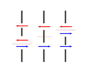
Depending on the position of the neutral level relative to the openings, the flow through a sash window has three regimes, as depicted in figure 3. In the first regime, the neutral level is located at the lower window, i.e.  $0 < \hat {z}_n < \beta$, leading to a bidirectional flow through the lower opening (figure 3a). In the second regime, the neutral level is located within the closed section of the window, i.e. $\beta \leq \hat {z}_n \leq (\beta + \alpha )$, leading to unidirectional flow through each opening (figure 3b). The third regime corresponds to the situation where the neutral level is located at the upper window, i.e. $(\beta + \alpha ) < \hat {z}_n < 1$, in which case a bidirectional flow occurs at the top opening (figure 3c).
Flow regimes through a sash window: (a) bidirectional flow at the lower window, (b) unidirectional flow and (c) bidirectional flow at the upper window. In each case the interior space is on the right.

2.1 Semi-analytic model
We derive a semi-analytic model for the flow rate through a sash window, given a particular window geometry ( $\alpha$ and $\beta$) and temperature difference. The flow velocity is given by (2.2), and the ventilation rate is equal to the flow velocity integrated over the area above or below the neutral pressure height
 \begin{equation} Q = \int_{\hat{z}_n}^1 H W C_d v(\hat{z}) \,\mathop{}\!\mathrm{d} \hat{z} = \int_{0}^{\hat{z}_n} H W C_d v(\hat{z}) \,\mathop{}\!\mathrm{d} \hat{z}, \end{equation}
with  $C_d$ the discharge coefficient accounting for streamline contraction and friction at the opening. We will discuss the value of $C_d$ in § 3. By equating the two expressions in (2.3), we can calculate $\hat {z}_n$ and therefore $Q$.
$Q$.
For bidirectional flow at the lower window ( $0 < \hat {z}_n < \beta$), integrating only over the open areas of the window
 \begin{align} Q & = \sqrt{2g'H}C_d \int_{\hat{z}_n}^\beta W H ( \hat{z} - \hat{z}_n )^{1/2} \,\mathop{}\!\mathrm{d} \hat{z} + \sqrt{2g'H}C_d \int_{\beta + \alpha}^1 W H ( \hat{z} - \hat{z}_n )^{1/2} \,\mathop{}\!\mathrm{d} \hat{z}\nonumber\\ & = \sqrt{2g'H}C_d \int_{0}^{\hat{z}_n} W H ( \hat{z}_n - \hat{z} )^{1/2} \,\mathop{}\!\mathrm{d} \hat{z}. \end{align}
Here, the outflow through the upper part of the window is split between the upper window and the upper part of the lower window. For unidirectional flow at both windows ( $\beta \leq \hat {z}_n \leq \beta + \alpha$), the ventilation rate is given by
 \begin{equation} Q = \sqrt{2g'H}C_d\int_{\beta + \alpha}^1 W H ( \hat{z} - \hat{z}_n )^{1/2} \,\mathop{}\!\mathrm{d} \hat{z} = \sqrt{2g'H}C_d\int_{0}^{\beta} W H ( \hat{z}_n - \hat{z} )^{1/2} \,\mathop{}\!\mathrm{d} \hat{z}. \end{equation}
When there is bidirectional flow at the upper window ( $\beta + \alpha < \hat {z}_n < 1$), the ventilation is given by
 \begin{align} Q& = \sqrt{2g'H}C_d\int_{0}^{\beta} W H ( \hat{z}_n - \hat{z} )^{1/2} \,\mathop{}\!\mathrm{d} \hat{z} + \sqrt{2g'H}C_d\int_{\beta + \alpha}^{\hat{z}_n} W H (\hat{z}_n - \hat{z})^{1/2} \,\mathop{}\!\mathrm{d} \hat{z}\nonumber\\ & = \sqrt{2g'H}C_d\int_{\hat{z}_n}^1 W H ( \hat{z} - \hat{z}_n )^{1/2} \,\mathop{}\!\mathrm{d} \hat{z}. \end{align}
 The height of the lower window at which the transition occurs from a uni- to a bidirectional flow at the upper window is denoted by  $\beta _{crit}$. To determine, for a given geometry $(\alpha, \beta )$, which flow regime occurs we solve (2.6) numerically for $\hat {z}_n = \alpha + \beta _{crit}$. After simplification this amounts to solving
 \begin{equation} (1-\alpha-\beta_{crit})^{3/2} + \alpha^{3/2} - (\alpha + \beta_{crit} )^{3/2} = 0, \end{equation}
for  $\beta _{crit}$. For a given geometry $(\alpha, \beta )$, comparing $\beta$ with the obtained value for $\beta _{crit}$ will determine which of (2.4), (2.5) or (2.6) to consider. After determining the flow regime, the associated volume conservation equation can be solved for $\hat {z}_n$ and $Q$.
$Q$.
Figure 4 depicts the variation of the normalised flow rate  $Q/Q_0$ versus the height of the lower opening normalised by the open area, $\beta /(1-\alpha )$, for different $\alpha$. For a given height $\alpha$ of the closed panel, $1-\alpha$ corresponds to the maximum value for $\beta$. The ventilation rate $Q$ is normalised by $Q_0$, the flow rate through an open rectangular window of dimension $W \times H$. In this case, due to conservation of mass, the neutral pressure level is at the mid-height of the window, $\hat {z}_n = 1/2$. Similarly to Reference Brown and SolvasonBrown and Solvason (Reference Brown and Solvason1962), we obtain the ventilation rate $Q_0 = \frac {1}{3}WHC_d\sqrt {g'H}$ by integrating (2.3) over half the window. For a given $\alpha$, small values of $\beta$ (dashed lines) lead to a bidirectional flow at the upper window. Enlarging the height of the lower window will result in a unidirectional flow through both openings (solid lines). Increasing $\beta$ further will cause the transition from uni- to bidirectional flow at the lower window (dotted lines). Due to the symmetry of the sash window, the variation of the flow rate with $\beta /(1-\alpha )$ is symmetric. Moreover, when $\alpha$ increases, the flow rate through the sash window decreases and the range of $\beta /(1-\alpha )$ corresponding to the unidirectional flow regime increases.
The variation of the ventilation rate predicted by the semi-analytic model with the height of the lower opening normalised by the open area,  $\beta /(1-\alpha )$: bidirectional flow regime at the upper window (thick dashed line), unidirectional flow regime (thick solid line), bidirectional flow regime at the lower window (thick dotted line). The flow rates predicted by the analytic model for the transition from one flow regime to another are plotted ( $\diamondsuit$).

In many circumstances a user may wish to maximise the flow rate. From figure 4 we can see that the flow is maximised when the height of the upper and lower windows are the same, i.e.  $\beta = {(1-\alpha )}/{2}$, with the neutral level located at the middle of the sash window, i.e. $\hat {z}_n = \beta +{\alpha }/{2}$. The maximum flow rate $Q_{max}$ can be expressed as a function of the geometry of the sash window using (2.5),
 \begin{equation} Q_{max}(\alpha) = Q_0 \times (1 - \alpha^{3/2}), \end{equation}
i.e. a sash window will have a maximum ventilation rate reduced by a factor of  $1 - \alpha ^{3/2}$ compared with a rectangular window of the same height and width. Looking at the pressure profiles in figure 2 the ventilation rate is thus maximised when the effective pressure difference is maximised by maximising the distance between the openings and the neutral level. For $\alpha = 0.5$, the flow rate through a sash window is 65 % of the flow rate if half the window were not filled with a sash.
The minimum flow rate,  $Q_{min}$, is obtained when one of the openings is closed (figure 4). When the upper opening is closed, (2.4) gives
 \begin{equation} Q_{min}(\alpha) = Q_0 \times (1 - \alpha)^{3/2}. \end{equation}
 Figure 5 depicts the variation with  $\alpha$ of the ratio of maximum to minimum flow rate obtained from (2.8) and (2.9). The ratio increases with $\alpha$, i.e. the difference between the maximum and minimum flow rate for a sash window increases with the size of the closed panel. For $\alpha = 0.5$ the maximum ventilation rate is less than twice the minimum one, while for $\alpha = 0.8$ the maximum flow rate is around three times larger than the minimum flow rate.
Variation with  $\alpha$ of the ratio of maximum to minimum ventilation rate for a sash window with constant temperature difference ( $Q_{max} / Q_{min}$) and the ratio of the temperature difference for a fully open window and sash window with a constant heat source $(\widetilde {\Delta T} / \Delta T )|_{max}$.

2.2 Constant internal heat source: summertime ventilation
During summertime a primary reason for ventilation is to provide cooling. Internal heat is produced by solar gains, occupants and appliances. While the strength of these heat sources can vary with time, for the sake of simplicity we consider the case of a room containing a heat source of constant strength  $W_h$ at floor level. Similarly to Reference Fitzgerald and WoodsFitzgerald and Woods (Reference Fitzgerald and Woods2007) and Reference Livermore and WoodsLivermore and Woods (Reference Livermore and Woods2007), assuming that the radiant heat losses are minimised and the room is well insulated, the heat supplied at the floor matches that lost through ventilation,
 \begin{equation} W_h = \Delta T c_p \rho Q = \widetilde{\Delta T} c_p \rho \tilde{Q}, \end{equation}
where  $c_p$ is the specific heat capacity of air and $\tilde {Q}$ and $\widetilde {\Delta T}$ are the ventilation rate and outdoor–indoor temperature difference for the equivalent fully open window of area $W \times H(1-\alpha )$. The ventilation rate through this opening is $\tilde {Q}^{3/2} = Q_{min} Q^{1/2}$, where (2.10) has been used to substitute for $\widetilde {\Delta T}$. With some rearranging we find the ratio $Q/\tilde {Q} = (Q/Q_{min})^{2/3}$. This is equivalent to $\widetilde {\Delta T}/\Delta T = (Q/Q_{min})^{2/3}$. We can interpret this as the cooling potential of a sash window (which maintains the room at $\Delta T$ higher than the outdoor temperature) compared with the cooling potential of a single opening of the same open area (which has a temperature difference of $\widetilde {\Delta T}$ with outdoors, $\widetilde {\Delta T} > \Delta T$). The maximum value of this temperature ratio is
 \begin{equation} \left.\frac{\widetilde{\Delta T}}{\Delta T}\right|_{max} = \frac{(1-\alpha^{3/2})^{2/3}}{(1-\alpha)}. \end{equation}
This function is plotted against  $\alpha$ in figure 5 and indicates the factor by which the temperature difference with outside can be reduced if the room is ventilated using a sash window with two openings rather than a single opening of the same total opening height. For $\alpha = 0.5$, the indoor–outdoor temperature difference for a fully open window is approximately $50\,\%$ larger than that maintained by a sash window with upper and lower openings of the same height, while for $\alpha = 0.9$ the temperature difference more than doubles.
2.3 Analytic model
As an alternative to the model presented in § 2.1, we derive a model to predict the flow rate through a sash window analytically. This analytic model takes for input  $\alpha$, the height of the closed panel, and $\hat {z}_n$, the position of the neutral layer as a function of the sash window geometry. The flow regime is directly given by the expression of $\hat {z}_n$ and thus the volume conservation equation is not solved numerically and the height of the openings of the sash windows are functions of the initial parameters. This analysis also reveals an analytic alternative to (2.7) for calculating $\beta _{crit}$.
For the bidirectional flow regime at the upper open panel when the neutral level is located at the upper opening, (2.6) simplifies to
 \begin{equation} \hat{z}_n^{3/2} - (\hat{z}_n - \beta)^{3/2} + (\hat{z}_n - \alpha -\beta)^{3/2} - (1 -\hat{z}_n)^{3/2} = 0. \end{equation}
Writing  $\hat {z}_n = \alpha +\beta + \delta$, where $\delta \in [0,\frac {1}{2}(1-\alpha -\beta )]$ denotes the distance between the bottom of the upper window and the position of the neutral level, we have
 \begin{equation} (\alpha + \beta + \delta)^{3/2} - (\alpha + \delta)^{3/2} - (1 - \beta - \alpha - \delta)^{3/2} + \delta^{3/2} = 0. \end{equation}
Assuming that  $\beta + \delta \ll 1 - \alpha$ and $\beta + \delta \ll \alpha$, the Taylor expansion of (2.13) results in the following expression for $\beta$:
 \begin{equation} \beta \approx \frac{2}{3} \times \frac{(1 - \alpha)^{3/2} + (\alpha + \delta)^{3/2} - \alpha^{3/2} - \delta^{3/2}}{\alpha^{1/2} + (1-\alpha)^{1/2}} - \delta. \end{equation}
Thus, by assuming a relative position for the neutral level, the height of the upper and lower openings are expressed as functions of  $\alpha$ and $\delta$. For $\delta = 0$, the flow transitions from uni- to bidirectional at the upper window. The associated height for the lower opening $\beta _{crit}^*$ is
 \begin{equation} \beta_{crit}^ * \approx \frac{2}{3} \times \frac{(1 - \alpha)^{3/2}}{\alpha^{1/2} + (1-\alpha)^{1/2}}. \end{equation}
Due to the symmetry of the problem, a similar approach can be conducted for the bidirectional flow regime at the lower window. The role played by the heights of the two openings for this regime will be inverted compared with the bidirectional flow regime at the upper window, with the critical  $\beta$ equal to $1-\alpha -\beta _{crit}^*$.
In figure 4 the critical height and flow rate predicted by the analytic model for the transition from one regime to another is plotted (diamonds). At the transition from one regime to another, the two models show a good agreement for the critical height and the flow rate. Indeed the relative difference for the flow rate is less than  $2.5\,\%$.
The evolution, with  $\alpha$, of $\beta / (1-\beta -\alpha )$ at the transition from uni- to bidirectional flow at the upper window is depicted in figure 6 and used to compare the two models. Using the analytical values $\beta _{crit}^*$ as well as those predicted by the semi-analytic model, $\beta _{crit}$, the ratio corresponds to the ratio of the height of the lower opening to the upper one. For the semi-analytic model the transition from one flow regime to another is obtained by solving (2.7) numerically. The difference between the two models is less than $1.2\,\%$, supporting the assumptions made in the analytic model for the Taylor expansion.
Ratio of upper and lower opening heights  $\beta _{crit} / (1-\alpha -\beta _{crit})$ with $\alpha$ for the transition from the uni- to the bidirectional flow regime at the upper window. The values, $\beta _{crit}$ (solid line), obtained from the semi-analytic model are compared with the analytical ones, $\beta _{crit}^*$ (dashed line).

Furthermore, it is interesting to observe that the transition from uni- to bidirectional flow occurs at a smaller ratio of lower and upper openings as the total opening area decreases. For  $\alpha =0.5$, the transition from a unidirectional to a bidirectional flow regime at the upper window regime occurs when the lower window area is half of the upper window. For $\alpha = 0.85$, transition occurs at a ratio of $0.25$.
3. Experimental set-up
In order to test the models developed, we performed small-scale experiments using fresh and salt water. The experimental set-up is sketched in figures 7(a) and 7(b). The tank had dimensions  $0.58\ \textrm {m} \times 0.58\ \textrm {m}\times 0.59\ \textrm {m}$ with a barrier dividing the tank into two equal compartments. An opening in the barrier acted as a window, with a width of $w_b =0.1\ \textrm {m}$ and a height of $h_b = 0.21\ \textrm {m}$. As depicted in figure 7(b), an aluminium mask was applied over the window opening to obtain a sharp-edged sash window of height $H = 0.16\ \textrm {m}$ and of width $W = 0.05\ \textrm {m}$. This mirrors the height-to-width ratio of a full-scale sash window, which usually lies between 2 and 4. The initial density difference $\Delta \rho$ was equal to $0.081 \pm 0.004\ \textrm {g}\ \textrm {cm}^{-3}$, i.e. with a maximal error of $5\,\%$, for all the experiments. The ratio $\Delta \rho /\rho$ was kept lower than $8\,\%$, such that the Boussinesq approximation was valid.
Views of the experiments: (a) top view of the tank, (b) the sash window mask applied on the window inside the barrier,  $W = 0.05$ m and $H = 0.16$ m. The dimensions are given in millimetres.

Defining  $h$ as $h_u$ or $h_l$, respectively, the Reynolds number at the upper, or lower, opening is given by $Re = {\min (h,W)}/{\nu } \times \sqrt {g'h}$. For all experiments, $Re > 1200$ and we assumed a constant discharge coefficient. Indeed Reference KielKiel (Reference Kiel1991) showed experimentally that the discharge coefficient of a flow through an orifice remains constant for $1000 < Re < 15\,000$ and Reference BotBot (Reference Bot1983) showed that for full-scale experiments the discharge coefficient is not dependent on the Reynolds number but can change with the aspect ratio. Applying the equation for the discharge coefficient as a function of the aspect ratio, derived by Reference BotBot (Reference Bot1983), to our experiment suggests that the variation is less than 1.5 %. Some initial experiments were performed with an opening of $0.10\ \textrm {m}\times 0.10\ \textrm {m}$ in the barrier between the two compartments. We measured the discharge coefficient $C_d = 0.69$ and used this value for the remainder of our experiments. The value obtained for the discharge coefficient is larger than the commonly accepted value of $0.6$ but other research obtained a discharge coefficient larger, e.g. Reference BotBot (Reference Bot1983) obtained a discharge coefficient between $0.64$ and $0.75$. Using hydraulic theory for a rectangular opening, Reference Dalziel and Lane-SerffDalziel & Lane-Serff (Reference Dalziel and Lane-Serff1991) observed for the discharge coefficient an increase of $20\,\%$ between a doorway geometry and that of a window. A similar increase is observed between the discharge coefficient of $0.57$ measured by Reference Frank and LindenFrank and Linden (Reference Frank and Linden2014) for a doorway and the one we measured for a window in the same tank ( $+21\,\%$).
If the two tanks are initially filled to the same height this would result in an initial flow of dense fluid through the sash window until the steady state of the system is reached. From (2.1), to minimise the unidirectional flow we fill the fresh water tank to a greater depth than the salt water tank in order to have the neutral level start at its steady-state height thereby limiting unbalanced flow between the two compartments.
A typical experiment consisted of the following steps. First, one compartment was filled with fresh water of density  $\rho _{i,0}$ and the other compartment was filled with salt water of density $\rho _{e,0}$. These densities were measured using a density meter (Anton-Paar, DMA 5000) with an accuracy of $10^{-6}\ \textrm {g cm}^{-3}$. The window was opened for a given runtime, $\Delta t$. After the gate was closed, the liquid in each compartment was thoroughly mixed for two minutes. The new densities $\rho _{i,1}$ and $\rho _{e,1}$ were measured. Assuming that the flow rates were constant between the two compartments and that the volume of water on each side did not change, the flow rate from one compartment to another can be obtained from the measured densities. The height of fluid in each tank remained similar before and after the experiment, with the variation of volume of liquid in each compartment being smaller than $1\,\%$ for every experiment. To reduce the experimental error, the final experimental flow rate is the average of the flow rates from one tank to another. The experiment was backlit with a projector at a distance of $1.5$ m from the tank wall, using a $45^\circ$ mirror. The light passing through the experiment was nearly parallel and was projected onto a sheet of tracing paper on the camera side of the tank. This technique, known as shadowgraph (Reference MowbrayMowbray, 1967) was used for flow visualisation (figure 7a).
3.1 Determination of  $\Delta t$

The runtime  $\Delta t$ of each experiment was between $15$ and $30$ s depending on the geometry considered for the sash window. For each experiment, $\Delta t$ was chosen to limit the error in the measured flow rate. During the experiment the dense water flows through the sash window and creates a dense layer at the bottom of the compartment with the initially light fluid. Similarly, the light fluid flows through the sash window and accumulates at the top of the compartment with the initially dense liquid. Since the sash window is nearer the bottom of the tank than the free surface, the bottom dense fluid layer is the first to interact with the sash window. The maximum runtime $\Delta t$ was determined for each sash window geometry to limit the interaction of this dense layer with the flow through the sash window, i.e. to limit the change of the effective density difference across the lower opening during the experiments. To determine the density profile next to the window, an initial set of experiments was run for each case, varying the runtime. For each of these experiments, the density profile alongside the window was measured $2$ minutes after the barrier was closed, when the flow had stabilised. A longer $\Delta t$ is desired as it reduces the error in the measured flow rate. Therefore the runtime was maximised while keeping the change in density difference at the base of the window less than $10\,\%$.
3.2 Experimental flow rate
To measure the flow rate,  $Q_{exp}$ through the sash window using the initial ( $\rho _{i,0}$ and $\rho _{e,0}$) and the final ( $\rho _{i,1}$ and $\rho _{e,1}$) densities in each compartment we assumed that the flow rates were constant and equal during the runtime $\Delta t$. In this case,
 \begin{equation} Q_{exp} = \frac{1}{2} \left( \frac{V_{i}}{\Delta t}\times \frac{\rho_{i,1} - \rho_{i,0}}{\rho_{e,0} - \rho_{i,0}} + \frac{V_{e}}{\Delta t}\times\frac{\rho_{e,1} - \rho_{e,0}}{\rho_{i,0} - \rho_{e,0}} \right), \end{equation}
where  $V_i$ and $V_e$ are the volume in each compartment at the beginning of the experiment. For each sash window geometry considered, at least four experiments were conducted and we calculated the mean flow rate $\bar {Q}$. The error in the flow rate shown as error bars in the figures 10(a) and 10(b) calculated for each geometry takes into account the measurement errors related to the runtime, the densities and the volume of liquid in each compartment.
4. Results and discussion
In this section we compare the results from the experiments with the prediction from the semi-analytic model. Two sets of experiments were performed to test and validate the models: varying  $\beta$ while keeping $\alpha$ constant and varying $\alpha$ with $\beta = 1 - \alpha - \beta _{crit}$.
4.1 Different flow regimes for $\alpha = 0.5$

In the first set of experiments, the height of the closed panel is fixed ( $\alpha = 0.5$) and the height of the lower window is varied to consider the three different flow regimes, $\beta \in \{0.420 ; 0.250 ; 0.080\}$, and the transitions from one regime to another, $\beta \in \{0.333 ; 0.168\}$ (table 1). Figure 8 shows the shadowgraphs of the dense flow through the sash window for $\alpha = 0.5$, and $\beta \in \{0.420 ; 0.250 ; 0.080\}$. The vertical black lines delimit the opening of the sash window. Movies of three experiments with $\alpha = 0.5$ and varying $\beta$ are available (see supplementary movies at https://doi.org/10.1017/flo.2021.14). As expected, we observe in figure 8(a) a bidirectional flow at the lower window, while when the height of the lower window is decreased to $\beta = 0.250$ a unidirectional flow is observed (figure 8b). When the height of the lower window is decreased to $\beta = 0.080$, there is a bidirectional flow at the upper window (figure 8c). Due to the density of the fluid, the dense flow through the upper window mixes with the flow through the lower window.
Shadowgraphs of the dense flow through the sash window for  $\alpha = 0.5$ at $t = 3.5$ s. The geometry of the sash window is delimited by the black lines on the left. The figures have been mirrored to be consistent with figure 2. The three different regimes are captured: (a) bidirectional flow at the lower window ( $\beta = 0.420$), (b) unidirectional flow ( $\beta = 0.250$) and (c) bidirectional flow at the upper window ( $\beta = 0.080$).

Runtime and number of runs for the different sash window geometries considered. Set 1 corresponds to the different geometry considered for  $\alpha =0.5$, while set 2 corresponds to the transition from the unidirectional to the bidirectional flow regime at the lower window, $\beta = 1 - \alpha - \beta _{crit}^*$. The first experiment of set 2 is also used in set 1.

Figure 9 depicts the flow of light and dense fluids through the sash window at  $t = 11.25$ s for $\alpha = 0.5$ and $\beta = 0.420$. Due to the fact that only one of the two compartments was visualised, the same experiment was conducted twice, swapping the dense and light liquids in the two compartments. As predicted by the semi-analytic model for this geometry of the sash window, a bidirectional flow regime is observed at the lower window while only light fluid is flowing through the upper window. The layer of dense fluid at the bottom of the tank with initially light fluid can be observed in figure 9(b).
Shadowgraphs of the flow through the sash window for  $\alpha = 0.5$ and $\beta = 0.420$ at $t = 11.25$ s. A bidirectional flow regime at the lower window is captured. (a) Light flow in the dense compartment and (b) dense flow in the light compartment.

Figure 10(a) shows the variation of the flow rate through the sash window for  $\alpha = 0.5$ when the height of lower window is changed. The semi-analytic prediction for the flow rate is also plotted. Each experimental result is the average of five to eight experiments. Overall the results from the semi-analytic model and from the experiments show a good agreement.
Variation of the normalised flow rate,  $\bar {Q} /\ Q_0$ predicted by the semi-analytic model (line) and measured experimentally (circles): (a) variation with $\beta / (1 - \alpha )$ for $\alpha = 0.5$ and (b) variation with $\alpha$ for the transition from the unidirectional flow to the bidirectional flow regime at the lower window. Error bars are calculated from $\sigma /\sqrt {n}$, where $\sigma$ is the root mean square of experimental uncertainties associated with each run and $n$ is the number of experiments for a particular case.

A slight under prediction by the model of the measured flow rate can be seen at high and low values of  $\beta /(1-\alpha )$ (there is a $6\,\%$ difference at $\beta /(1-\alpha ) = 0.16$). The reader might assume the discrepancy occurs due to mixing at the interface of the bidirectional flow at the upper window, but this effect would be expected to reduce the measured flow rate below the prediction of the model. Furthermore the small change in volume due to a short early period of unidirectional flow (when the neutral buoyancy height adjusts to a steady state), would only be expected to change the measured flow rate by less than $1\,\%$. One possible partial explanation for the difference is a small change in the discharge coefficient through the smaller openings that exist for high or low $\beta /(1-\alpha )$, which could be due to the difference in aspect ratio of the openings.
4.2 Flow regime transitions for different $\alpha$

In the second set of experiments, we varied  $\alpha$ and selected $\beta$ so that the flow was at the transition from the uni- to the bidirectional regime at the lower window (table 1). The runtime increases with the increase of $\alpha$, as the sash window open area shrinks, leading to a decrease in the flow rate.
Figure 10(b) depicts the variation of the flow rate measured experimentally for  $\alpha$ between $0.5$ and $0.7$ for the transition from the uni- to the bidirectional flow regime at the lower window ( $\beta = 1 - \alpha - \beta _{crit}^*$). Each result is the average of four to eight experiments. The prediction of the semi-analytic model for the flow rate is also plotted. We observe a good agreement between the experiments and the model.
5. Conclusions
We developed two models, the analytic one is used to predict  $\beta _{crit}$ while the semi-analytic model predicts the ventilation rates of a closed room with the flow driven by a temperature difference between indoors and outdoors through a sash window. Depending on the geometry of the window openings, three different flow regimes can be observed, leading to different flow rates. For large lower openings a bidirectional flow at the lower window occurs. When this height is decreased to a critical value, a unidirectional flow regime occurs at both openings with inflow of cold exterior air through the lower opening and outflow of warm indoor air through the upper opening. Continuing to decrease the height of the lower opening, the flow transitions from uni- to bidirectional at the upper opening. The comparison of the predicted critical window height for transition between the semi-analytic and the analytic model validates the assumptions made to create the analytic model. Furthermore, the small-scale experiments conducted in a water tank confirm the transitions between the different flow regimes and the flow rates associated with the different sash window geometries.
By using these models we now make some estimates of typical ventilation rates. If we consider a room with a volume of  $25\ \textrm {m}^3$ and a typical sash window of $1\ \textrm {m} \times 0.5\ \textrm {m}$, from the temperature difference between the inside and the outside we can estimate the flow rate and therefore the ventilation of the room. We assume that the room has a temperature of $25\,^{\circ} \textrm {C}$ and there is a temperature difference of $5\,^\circ \textrm {C}$ with the outside. If the opening of the sash window is maximal ( $\alpha = 0.5$) and the heights of the upper and lower windows are the same ( $\beta = 0.25$) then the flow rate through the sash window estimated by the semi-analytic model equals $Q \approx 2.63 \times 10^{-2}\ \textrm {m}^3\ \textrm {s}^{-1}$ (using $C_d = 0.6$), which corresponds to an air change rate for this assumed room volume of $3.8$ air changes per hour (ACH). Keeping the height of the closed panel constant, if the height of the lower panel increases to $\beta = 0.4$, the flow rate decreases to $2.61$ ACH. Reaching the case where the upper window is closed and only the lower window is open, the air change rate decreases to $2.07$ ACH. An even more dramatic difference would occur if the total open area of the sash window was smaller ( $\alpha > 0.5$), with the ventilation rate being more sensitive to the geometry of the sash window. For $\alpha = 0.9$ the ratio of maximum to minimum flow rate is almost 4.8 (a reduction from 0.86 to 0.18 ACH).
The formulation of simple models to identify flow regimes and calculate ventilation rates is important for ventilation modelling. These new models can be used to design ventilation systems in low energy buildings, for research and building energy models, and integrated into programs controlling the ventilation of smart buildings.
Acknowledgements
We would like to thank the technical staff in the G. K. Batchelor Laboratory, and particularly D. Page-Croft.
Funding Statement
This work is supported by the Engineering and Physical Sciences Research 395 Council (EPSRC) Grand Challenge grant Managing Air for Green Inner Cities (MAGIC) (grant number EP/N010221/1).
Declaration of Interests
The authors declare no conflict of interest.
Data Availability Statement
Raw data are available from the corresponding author (G.K.).
Ethical Standards
The research meets all ethical guidelines, including adherence to the legal requirements of the study country.
Supplementary Movies
Supplementary material and movies are available at https://doi.org/10.1017/flo.2021.14.


 Open access