


Impact Statement
The ocean constitutes a major component of the Earth's carbon cycle, having taken up around a quarter of human-made emissions to date. Despite taking up a very small area of the ocean, seaweeds such as kelp have very high rates of primary production per unit area. However, the amount of seaweed carbon that is stored in sediments and the deep ocean remains highly uncertain.
Here, we build a new model to capture the coupled flow/kelp interaction and we use this model to quantify the transport and release rate of a saturating tracer. Using a series of controlled numerical experiments, we find that there is a kelp density which maximises tracer release. These insights will help us understand the role of natural kelp forests in the carbon cycle and could help inform strategies for effective seaweed aquaculture. This work also emphasises the importance of understanding the influence of smaller-scale physical processes on carbon storage and growth potential associated with kelp forests.
1. Introduction
Macroalgae occupy less than 1 % of the global ocean area but contribute up to 3.6 % of the global ocean primary productivity and potentially sequester up to 10 % of the carbon stored in the ocean (Reference Krause-Jensen and DuarteKrause-Jensen & Duarte 2016, henceforth Reference Krause-Jensen and DuarteKJ16). This outsized contribution is due to a combination of macroalgae's extremely fast growth rate, occupation of nutrient-rich coastal waters, particularly in upwelling areas, and high efficiency of nutrient utilisation (Reference DavisDavis 1991). Despite these estimates, significant uncertainty surrounds the fate of carbon exported from the system (Reference Krause-Jensen, Lavery, Serrano, Marba, Masque and DuarteKrause-Jensen et al. 2018) and the carbon sequestration potential of macroalgae ecosystems (Reference Gallagher, Shelamoff and LaytonGallagher, Shelamoff & Layton 2022).
Macroalgae continually export carbon, both dissolved in the water (Reference Reed, Carlson, Halewood, Clinton Nelson, Harrer, Rassweiler and MillerReed et al. 2015) and as particulate detritus through erosion and breakage (Reference Krumhansl and ScheiblingKrumhansl & Scheibling 2012; Reference De Bettignies, Wernberg, Lavery, Vanderklift, Gunson, Symonds and CollierDe Bettignies et al. 2015). Since the majority of benthic macroalgae grow in shallow waters with hard or sandy substrate, only a small fraction ( $\sim$0.4 %) of this carbon is stored in sediments or in the deep ocean (Reference Duarte and CebriánDuarte & Cebrián 1996; Reference Krause-Jensen and DuarteKJ16). One element of uncertainty in estimates of carbon storage by macroalgae is the fate of the exported dissolved and particulate carbon. Once the carbon has left the kelp forest, its destination will strongly influence the sequestration time. Carbon that is transported to the deep ocean can remain isolated from the atmosphere for hundreds of years (Reference Rousselet, Cessi and ForgetRousselet, Cessi & Forget 2021; Reference Siegel, Devries, Doney and BellSiegel et al. 2021), while carbon that becomes buried in sediment can be stored for geological time scales (Reference Teng and ZhangTeng & Zhang 2018).
In addition to uncertainties in carbon storage, the interaction of macroalgae and the remainder of the ecosystem is complex and not fully understood. For example, the modification of alkalinity in and around kelp forests is of interest as climate change acidifies the ocean (Reference TraigerTraiger et al. 2022), but the biological effect can often be obscured by the physical environment (Reference Hirsh, Nickols, Takeshita, Traiger, Mucciarone, Monismith and DunbarHirsh et al. 2020). An important area where improving this understanding is vital is when considering kelp re- and afforestation which have been proposed as potential carbon dioxide removal strategies (National Academies of Sciences Engineering and Medicine 2022). Fully understanding these systems and their broader ecosystem effects is especially important in this context in order to mitigate undesirable knock-on effects. A better understanding of kelp forest/flow interactions could also help to optimise regrowth efforts to maximally enhance ecosystems, and minimise limitations such as nutrient depletion within kelp forests. Additionally, an improved understanding of the small-scale physical processes involved in the kelp forest/flow interactions will help inform parameterisations for larger-scale ocean models.
Observations and models of kelp forests are hindered by the vastly multi-scale nature of the physics and biogeochemistry. In this context, process-based understanding is useful to decipher observations and improve models (Reference Koweek, Nickols, Leary, Litvin, Bell, Luthin, Lummis, Mucciarone and DunbarKoweek et al. 2017). Given the sparsity of current observations, an effective step towards this will be improved modelling and data assimilation, a common technique for constraining process-based models with sparse observations (Reference BannisterBannister 2017).
The biogeochemical modelling of kelp forests has received some attention (e.g. Reference JacksonJackson 1987; Reference Burgman and GerardBurgman & Gerard 1990), while the physics remains an important and relatively unexplored area. Previous work has used field observations (Reference GaylordGaylord et al. 2007; Reference Gaylord, Denny and KoehlGaylord, Denny & Koehl 2008), laboratory experiments (Reference Rosman, Denny, Zeller, Monismith and KoseffRosman et al. 2013) and analytical–numerical methods (Reference Utter and DennyUtter & Denny 1996, henceforth Reference Utter and DennyUD96) to study the flow/structure interactions in a giant kelp forest. The laboratory experiments used by Reference Rosman, Denny, Zeller, Monismith and KoseffRosman et al. (2013) focused on the flow within the kelp forest. Here, we use an elastic model for the motion of giant kelp developed by Reference Utter and DennyUD96 and Reference Rosman, Denny, Zeller, Monismith and KoseffRosman et al. (2013) in a large-eddy simulation (LES) with coupled flow/kelp forest interactions. We apply this model to simulate tidal flow around and through an isolated kelp forest as an idealisation of the flow observed by Reference GaylordGaylord et al. (2007).
A central question that we address here is: How does the release or uptake of a dissolved substance by a kelp forest depend on the density of kelp within the forest? This is not a trivial question because, while increasing the kelp density increases the number of individuals able to consume or release a tracer, high kelp densities also restrict the flow through the kelp forest and reduce the volume of ambient water exposed to the kelp. Answering this question will provide insight into the influx of tracers such as nutrients into the kelp forest and the export of tracers such as dissolved inorganic carbon.
In this paper, we will first describe the formulation of a model of the motion of giant kelp (Macrocystis pyrifera) individuals and our implementation within a LES. We will then describe the calibration of the model parameters using ensemble Kalman inversion (Reference Iglesias, Law and StuartIglesias, Law & Stuart 2013) based on field measurements of the flow in and around a natural giant kelp forest. We then systematically vary the density of individuals within the kelp forest and attempt to disentangle the fluid dynamical influences on the uptake and export of tracers by the kelp. Finally, we use these insights to speculate on the growth limitations of natural kelp forests and recommend considerations related to the design of kelp farms.
2. Methods
2.1 Mathematical description
The work of Reference Utter and DennyUD96 modelled individual giant kelp as a single elastic line segment attached to a floating point mass which is subject to forces from buoyancy, tension, drag and the fluid pressure gradient. Reference Rosman, Denny, Zeller, Monismith and KoseffRosman et al. (2013) used the formulation of Reference Utter and DennyUD96 but discretised the kelp individual into multiple segments. This allowed the kelp to take on a complex shape (as opposed to previous models which assume one straight segment), which is likely to be an important factor in the kelp–flow interaction (Reference Tinoco, San Juan and MullarneyTinoco, San Juan & Mullarney 2020). We have modified their formulation and coupled the equations within a fluids solver.
Specifically, we model kelp as a series of nodes at positions  $\boldsymbol {x_i}$, connected with elastic line segments and attached to the bottom of the domain at a fixed point, $\boldsymbol {x_b}$, which serves as the origin for the frame of reference for the node positions. This is illustrated in figure 1. The motion of each node is given by
 \begin{equation} m_e\frac{{\rm d}^2\boldsymbol{x_i}}{{\rm d} t^2} = \boldsymbol{F^B} + \boldsymbol{F^D} + \boldsymbol{T^-} + \boldsymbol{T^ + } + \boldsymbol{F^I}. \end{equation}
Diagram of giant kelp structure, discretisation and forces.

Here,  $m_e$ is the effective mass (accounting for the kelp and the water moved along with the kelp) and is equal to $V_B\rho _m + V_P\rho _P + (V_B + V_P)C_a\rho _w$, where $V_B$ and $V_P$ are the volume of biomass (stipe and blades) and pneumatocysts (gas vesicles), respectively. The density is denoted $\rho _B$, $\rho _P$ and $\rho _w$ for the biomass, pneumatocysts and water, respectively. The added mass coefficient, $C_a$, is set by the amount of water that moves with the kelp. This was measured by Reference Gaylord, Blanchette and DennyGaylord, Blanchette & Denny (1994), who found $C_a=1.6\unicode{x2013}6.7$ for various species of macroalgae (not including M. pyrifera). The work of Reference Utter and DennyUD96 found that a value of $C_a=3$ gave the best agreement with measurements of the movement of M. pyrifera, and we use this value here. The values of other parameters and the sources used for the estimates are given in table 1.
Parameter values and sources.

The buoyancy force,  $\boldsymbol {F^B}$, is given by
 \begin{equation} \boldsymbol{F^B} = [(\rho_w - \rho_P)V_P + (\rho_w - \rho_B)V_B]\boldsymbol{g}\approx(\rho_w - \rho_P)V_P\boldsymbol{g}, \end{equation}
where  $\boldsymbol {g} = -g\boldsymbol {\hat {z}}$ is the acceleration due to gravity, and the second relation follows from assuming that the biomass component of the kelp is neutrally buoyant, i.e. $\rho _b \approx \rho _w$. The relative velocity, $\boldsymbol {u}_{rel}$ is $\boldsymbol {u}-\dot {\boldsymbol {x}}$, where $\boldsymbol {u}$ is the water velocity and $\dot {\boldsymbol {x}}$ is the node velocity. The drag force is then given by
 \begin{equation} \boldsymbol{F^D} = \tfrac{1}{2} \rho_W (C_{DS} A_S + C_{DB} A_B) |\boldsymbol{u}_{rel}|\boldsymbol{u}_{rel}. \end{equation}
Note that the drag is a three-dimensional vector whose direction is set by the differential motion of the kelp and the water ( $\boldsymbol {u}_{rel}$). Here, we treat the drag from the stipe and blades (which we consider to include the pneumatocysts in this context) as separate elements with different drag coefficients ( $C_{DS}$ and $C_{DB}$) with areas $A_S$ and $A_B$. The blade area is set to $A_B=3$ m $^2$ based on the typical blade area measured by Reference Jackson, James and NorthJackson, James & North (1985), and the drag coefficient is calibrated based on observational data reported in Reference GaylordGaylord et al. (2007), as described below. We treat the stipe as a solid cylinder with a projected area
 \begin{equation} A_S = 2r_sl|\sin\theta| + {\rm \pi}r_s^2|\cos\theta|, \end{equation}
where  $r_s$ is the stipe radius, $l$ the length of the section and $\theta$ the angle between the stipe and the flow. The stipe drag coefficient, $C_{DS}$, is set to $1$, which is typical for long cylindrical objects (Reference HoernerHoerner 1965) (and is also not important as the stipe drag is small compared with the fronds). The stipe length, $l$, is determined by calculating the distance between neighbouring nodes.
For the tension force, we use the same formulation as Reference Utter and DennyUD96, with the force given by
 \begin{equation} \boldsymbol{T^\pm} = \frac{\boldsymbol{\Delta x^\pm}}{|\boldsymbol{\Delta x^\pm}|}\begin{cases} k\left(\dfrac{|\boldsymbol{\Delta x^\pm}| - l_0^\pm}{l_0^\pm}\right)^\alpha A_C & \text{for } |\boldsymbol{\Delta x^\pm}| > l_0^\pm \\ 0 & \text{otherwise} \end{cases}, \end{equation}
where  $k$ is the spring constant and $\alpha$ is the spring exponent as determined by best fit to measurements by Reference Utter and DennyUD96. The parameter $l_0$ is the unstretched length, $A_C$ is the cross-sectional area of the stipe, ${\rm \pi} r_s^2$, and $\boldsymbol {\Delta x^\pm }$ is the distance between the considered node and the next/previous node.
Finally, the inertial (or acceleration) force resulting from the pressure gradient associated with the acceleration of fluid parcels is given by
 \begin{equation} \boldsymbol{F^I} = \rho_w (V_B + V_P)\boldsymbol{a}_w, \end{equation}
following Reference Utter and DennyUD96 and Reference Rosman, Denny, Zeller, Monismith and KoseffRosman et al. (2013), where  $\boldsymbol {a}_w$ is the fluid acceleration as measured in an inertial reference frame. This model neglects the stiffness of the stipes (i.e. reaction force to bending) but, as per previous models, this is reasonable since the bending force is small compared with other forces. According to Reference Gaylord and DennyGaylord & Denny (1997), the effective flexural stiffness is $\sim$10 N m $^{-2}$, and therefore the force imparted by stiffness when the kelp is deflected by the flow is approximately $150$ times smaller than the horizontal component of the elastic force (given a single 12 m element in 0.1 m s $^{-1}$ flow, resulting in a stretched length of $\sim$16 m and a deflection of 3.7 m).
2.2 Model implementation and calibration
We have implemented the above model in the active Lagrangian particle framework of OceanBioME.jl (Reference Strong-Wright, Chen, Constantinou, Silvestri, Wagner and TaylorStrong-Wright et al. 2023) and Oceananigans.jl (Reference Ramadhan, Wagner, Hill, Jean-Michel, Churavy, Souza, Edelman, Ferrari and MarshallRamadhan et al. 2020). To do this, we treat each kelp as a collection of ‘particles’ or ‘nodes’, each of which is advected by the local fluid velocity and subject to the forces described above.
2.2.1 Kelp dynamics model
Initially, we split the individuals into eight discrete segments (with nine nodes) in very high resolution ( $0.125\times 0.125\times 0.125$ m) LES tests. We configured our model to replicate the laboratory experiment of Reference Rosman, Denny, Zeller, Monismith and KoseffRosman et al. (2013) and reproduced very similar velocity profiles (shown in Appendix B). After this initial test, we reduced the kelp model to two segments (and three nodes) which, for lower-resolution models ( ${\sim }4\times 4\times 1$ m) gave very similar results to the eight-segment model. Typically one segment extends from the holdfast (fixed to the bottom) to the surface, representing the subsurface kelp, and the other segment floats on the surface, representing the kelp canopy. Since the kelp dynamical equations are much stiffer than the fluid equations, at each fluid integration sub-step we integrate the above system with a third-order Runge–Kutta–Wray integration (Reference Le and MoinLe & Moin 1991).
We apply the drag force from the discrete segments on the water by considering the drag to be shared equally between neighbouring grid cells. This typically leads to the segment from the base to the first node being distributed in a column of grid cells spanning the full water depth, while the segment between the first and second node applies drag to the surface cells. Additionally, the drag stencil was chosen to be only a single gridpoint in width since the horizontal cross-sectional area of kelp is much smaller than the horizontal area of our grid. Finally, to reduce the stiffness of the system, we added a linear damping term
 \begin{equation} -\frac{1}{\tau_d}\frac{{\rm d}\boldsymbol{x}}{{\rm d} t}, \end{equation}
to the equations for the kelp motion (2.1), with  $\tau _d = 1$ s. This value was chosen by trial and error as the largest value that keeps the model stable when constraining the timestep with the Courant–Friedrichs–Lewy (CFL) criterion. Note that $\tau _d$ is comparable to the time scale associated with the drag force, but is ${\sim }10$ times smaller than the period of elastic oscillations. By comparing simulations with and without this damping term, we found that including this term had no noticeable impact on the results, but significantly reduced the computational expense of the integration by allowing larger timesteps.
Most model parameters are taken from the existing literature, as shown in table 1. An exception is the drag coefficient, which depends on the morphology and orientation of the kelp fronds (Reference Utter and DennyUD96). We estimated the drag coefficient by comparing with measurements of flow speed in a giant kelp forest from (Reference GaylordGaylord et al. (2007), henceforth Reference GaylordG7) using ensemble Kalman inversion (EKI, Reference Iglesias, Law and StuartIglesias et al. 2013) with the EnsembleKalmanProcesses.jl package (Reference Dunbar, Lopez-Gomez, Garbuno-Iñigo, Huang, Bach and WuDunbar et al. 2022). We also used the inversion to constrain the background flow and the density variation within the kelp forest as described below.
Our computational domain is  $5\,{\rm km}\,{\times}\, 2\,{\rm km}$ in the horizontal directions and 8 m in the vertical direction, with $256$ regularly spaced gridpoints per kilometre in the horizontal ( ${\sim }3.9$ m resolution) and $1$ gridpoint per metre in the vertical direction. We apply periodic boundary conditions in both horizontal directions, a no-slip boundary condition at the bottom of the domain and a free-slip condition at the top of the domain.
We model the kelp forest as a 100 m radius circle, where each gridpoint inside the circle contains the anchor (holdfast) for a single kelp model. We are particularly interested in the influence of the density of kelp within the kelp forest on the kelp/flow interactions and the tracer exchange rates. To vary the density, we scale the drag and the tracer release rate by a density parameter,  $\sigma$, which sets the number of kelp individuals per square metre. However, we always use just one kelp model per gridpoint inside the kelp forest with the view that each kelp model represents the movement of a number of individuals. This significantly reduces the computational cost and since we do not model the direct interactions between individual kelp, this approach is reasonable.
Given that the average frond density measured in the summer by Reference GaylordG7 was  ${\sim }10$ frond m $^{-2}$ with ${\sim }20$ frond individual $^{-1}$, the corresponding kelp density is $\sigma =0.5$ individuals m $^{-2}$. Therefore, we scaled the drag of each of the model kelp to represent this individual density by the scale factor
 \begin{equation} \varSigma_0 = \sigma\Delta x\Delta y. \end{equation}
In order to replicate the smooth drop-off in density measured in the kelp forests Reference GaylordG7 we reduced the density at the edges using the functional form
 \begin{equation} \varSigma(r) = \varSigma_0 \tanh\left(\frac{r + 0.9r_f}{d}\right), \end{equation}
where  $r$ is the distance to the centre of the kelp forest, $r_f$ is the kelp forest radius and $d$ is a scale factor set through a process described below.
Our modelled kelp forest is subject to unidirectional semi-diurnal tidal currents. Since the kelp forest studied by Reference GaylordG7 is close to the shore, the tides are nearly rectilinear. We align the  $x$-axis with the along-shore direction, and let $y$ denote the cross-shore (cross-stream) direction. Following Reference Vreugdenhil, Taylor, Davis, Nicholls, Holland and JenkinsVreugdenhil et al. (2022), tides were implemented by applying a body force to the momentum equations of the form
 \begin{equation} \frac{\partial u}{\partial t} = {-}A_u\omega\sin(\omega t + \phi), \end{equation}
where  $A_u$ is the tidal amplitude, $\omega =1.41\times 10^{-4}$ rad s $^{-1}$ (the semi-diurnal tidal frequency) and $\phi =-({{\rm \pi} }/{2})$.
The work of Reference GaylordG7 reported measurements of flow magnitude and direction at several points around a giant kelp forest near Santa Barbara, California, along with speed ratios between points inside and outside the kelp forest. To calibrate our model, we compared the standard deviation of the time series of the velocity measured at fixed locations (stations) in and around the kelp forest (as a measurable correlated with the flow magnitude), and the velocity ratio gradient between stations (as a measurable correlated with the kelp forest drag), with data from Reference GaylordG7. The particular stations were chosen to be those with observed velocities most tangential to the shoreline to minimise the effect of shoreline geometry. The observations used for comparison are shown in Appendix A, and the position of the stations used for comparison are shown in figure 3. With these measurables, we calibrated the tidal amplitude ( $A_u$), the kelp forest density drop-off ( $d$) and the blade drag coefficient ( $C_{DB}$, since the blade drag is significantly larger than the stipe drag). For each generation, we ran ensembles of $12$ members for $2.5$ tidal cycles allowing the first half-cycle to be disregarded as a spinup. After $12$ generations of the calibration ensemble, the parameters had converged. This resulted in parameter values of $C_{DB}=0.87\pm 0.05$, $d=17\pm 6$ m and $A_u=0.102\pm 0.003$ m s $^{-1}$, which were used for subsequent experiments. Since the calibration is based on the velocity measured near and inside the kelp forest, a smaller domain size of $3\,{\rm km}\times 1\,{\rm km}\times 8\,{\rm m}$ was used for the calibration ensemble.
2.2.2 Large-eddy simulation configuration
The LES used here solves the incompressible Navier–Stokes equations under the Boussinesq approximation with the momentum evolution governed by
 \begin{equation} \frac{\partial\boldsymbol{u}}{\partial t} + \boldsymbol{u}\boldsymbol{\cdot} \boldsymbol{\nabla}\boldsymbol{u} = b\hat{\boldsymbol{g}} -\frac{\boldsymbol{\nabla} p}{\rho_0} - \boldsymbol{\nabla}\boldsymbol{\cdot}\boldsymbol{\boldsymbol{\tau}} + \boldsymbol{a_u}, \end{equation}
where  $\boldsymbol {u}$ is the velocity, $b$ is the buoyancy, $\hat {\boldsymbol {g}}$ is the vertical unit vector (pointing in the opposite direction to gravity), $p$ is the pressure (calculated by solving an elliptic Poisson equation derived from the divergence of the horizontal component of the momentum equation), $\rho _0$ is a constant reference density and $\boldsymbol {\nabla }\boldsymbol {\cdot }\boldsymbol {\boldsymbol {\tau }}$ is the divergence of the subgrid-scale stress tensor. The final term, $\boldsymbol {a_u}$, includes the tidal forcing and drag from the kelp
 \begin{equation} \boldsymbol{a_u} =
{-}\bigg(A_u\omega\sin(\omega t + \phi)\hat{\boldsymbol{x}}
+ \sum_i\left[\frac{w_i(x, y, z)}{2} (C_{DS, i} A_{S, i} +
C_{DB, i} A_{B, i}) |\boldsymbol{u}_{{rel},
i}|\boldsymbol{u}_{{rel}, i}\right]\bigg),
\end{equation}
\begin{equation} \boldsymbol{a_u} =
{-}\bigg(A_u\omega\sin(\omega t + \phi)\hat{\boldsymbol{x}}
+ \sum_i\left[\frac{w_i(x, y, z)}{2} (C_{DS, i} A_{S, i} +
C_{DB, i} A_{B, i}) |\boldsymbol{u}_{{rel},
i}|\boldsymbol{u}_{{rel}, i}\right]\bigg),
\end{equation}
where the sum is over all kelp nodes and  $w_i(x, y, z)$ is the fraction of the drag of kelp node $i$ applied at $x, y, z$. In the numerical implementation, the weight function, $w_i$, is defined discretely as the set of gridpoints nearest to the position of each node and the stipe connecting nodes $i$ and $i-1$. The drag force from kelp node $i$ is distributed equally among the gridpoints within this stencil. The tracer evolves according to
 \begin{equation} \frac{\partial C}{\partial t} + \boldsymbol{u}\boldsymbol{\cdot} \boldsymbol{\nabla} C = {-}\boldsymbol{\nabla}\boldsymbol{\cdot}\boldsymbol{q_c} + F_c, \end{equation}
where  $C$ is the tracer concentration, $\boldsymbol {\nabla }\boldsymbol {\cdot }\boldsymbol {q_c}$ is the divergence of the subgrid-scale flux and $F_C$ includes tracer uptake/release from the kelp as described below. For tracers released by the kelp, we modify $F_C$ in the grid cells neighbouring the kelp, using the same stencil used for the drag.
The subgrid-scale turbulence was modelled using the anisotropic minimum dissipation model (Reference Rozema, Bae, Moin and VerstappenRozema et al. 2015; Reference Vreugdenhil and TaylorVreugdenhil & Taylor 2018) which specifies  $\boldsymbol {\nabla }\boldsymbol {\cdot }\boldsymbol {\tau }$ and $\boldsymbol {\nabla }\boldsymbol {\cdot }\boldsymbol {q_c}$. We ran all simulations using a fifth-order upwind advection scheme to prevent oscillations associated with the localised drag and tracer release, a no-slip bottom boundary condition, a third-order Runge–Kutta–Wray time stepper (Reference Le and MoinLe & Moin 1991) and an adaptive time step with a CFL number of 0.8. Details of the numerical implementation can be found in Reference Ramadhan, Wagner, Hill, Jean-Michel, Churavy, Souza, Edelman, Ferrari and MarshallRamadhan et al. (2020) and associated documentation.
2.3 Experimental set-up
To determine the properties of the kelp forest that limit nutrient uptake (growth) and export, we conducted a series of 20 controlled numerical experiments where we varied the density of kelp within the kelp forest and kept all other parameters fixed. As a generalised representation of tracer uptake or release, the tracer forcing function is set to
 \begin{equation} F_c = {-}\frac{\varSigma}{\tau_r}(C - C_0). \end{equation}
In the absence of advection and diffusion, this forcing would cause the tracer concentration to saturate to the constant value  $C_0$ with a characteristic time scale, $\tau _r$. The time scale was selected to be 1 h as this is approximately equivalent to the uptake time scale of nutrients and blade loss rate in kelp (e.g. Reference FriederFrieder et al. 2022). This form is similar to the forcing often used for biogeochemical tracers such as nutrient concentration. Since the equation for $C$ is linear, the forcing applied to $C$ can be considered inverse uptake. Below, we will refer to ‘saturation’ as the percentage associated with the ratio ${C}/{C_0}$. The kelp forest density, $\sigma$, was varied between $0.25$ and $3$ individuals m $^{-2}$ with increments between $0.125$ and $0.25$ which adequately covers the range of observed kelp forests and more extreme values.
3. Results
3.1 Model calibration and kelp forest effect on flow
The density of individual kelp plants measured in Reference GaylordG7 varied from 0.11 individuals m $^{-2}$ in spring to $0.89$ individuals m $^{-2}$ in the summer. For our baseline case with a kelp density of $0.5$ individuals m $^{-2}$, the LES qualitatively reproduces the flow reported in Reference GaylordG7. An example of this is shown in figure 2 where the depth-averaged along-shore velocity is shown at four stages of the tidal cycle. The drag from the kelp forest generates a low-speed wake with arrows showing the flow direction, indicating that some of the flow is deflected around the kelp forest. In (b), in the slower wake region, the flow reverses earlier than the rest of the domain, generating a slightly higher peak velocity on the upstream side of the kelp forest. At this time the flow is inward on the left and right sides of the kelp forest, and as a result, the flow inside the kelp forest is directed outward in the $y$ directions. At a phase of ${\rm \pi} /4$ (c), the ambient flow away from the kelp forest has switched direction and is now moving to the left. The flow to the right of the kelp forest (what is now the upstream side) continues to lead the rest of the flow in phase. At a phase of $3{\rm \pi} /8$, the ambient velocity in the $x$ direction is close to its minimum and a low-speed wake has developed to the left of the kelp forest. The rest of the tidal cycle mirrors the behaviour in figure 2.
Depth-average along-shore velocity ( $u$) at various tidal phases, illustrating the time evolution of the flow around the kelp forest. The phase in radians is indicated in each panel, starting with a phase of zero in the first panel, defined as the time when the $x$-velocity forcing is zero. Arrows show the velocity averaged over a 40 m box.

We can compare figure 2 with figure 11 in Reference GaylordG7. They also note several features of the flow around the kelp forest which are observed here. They found a phase where the flow is convergent into the kelp forest in the along-shore direction with offshore flow from the kelp forest, similar to what we see in figure 2(b). They also observe a lack of a stable recirculation zone downstream of the kelp forest which would be expected behind a solid object. Notably, their observations showed a clear asymmetry due to the presence of the coastline, while our model set-up is symmetric.
Figure 3 shows a time series of the velocity in (b) at locations shown in (a), along with the ambient flow (in the absence of a kelp forest) indicated as a dashed line. The locations of the points were chosen to match measurement locations from Reference GaylordG7 as closely as possible. For the reference station (blue) it can be seen that the kelp forest shifts the phase of the tidal cycle, while for station 2 the damping when the station is downstream of the kelp forest is apparent as per Reference GaylordG7. The ratio of the velocities at these points was used to calibrate the drag coefficient by comparing with data reported in Reference GaylordG7 as described in § 2.2.1.
Panel (a) shows the position of the stations used for comparison with Reference GaylordG7. Panel (b) shows a time series of the depth-averaged velocity at these stations with a kelp density of 0.5 individuals m $^{-2}$. The first half of the tidal cycle should be disregarded as the model spins up.

As noted above, the density of the kelp forest measured by Reference GaylordG7 varies seasonally from 0.11 to 0.89 individuals m $^{-2}$. The density is also an important parameter in kelp farms. Following the calibration, we varied the kelp forest density from $0.25$ to $3$ individuals m $^{-2}$ with all other parameters held fixed. Figure 4 shows the flow speed, averaged in time and for all points inside the kelp forest as a function of kelp forest density. The depth-averaged and surface ( $z=0$) flows are both shown. This is due to the drag induced by the floating canopy of the kelp forest and is consistent with Reference Rosman, Denny, Zeller, Monismith and KoseffRosman et al. (2013). Notably even at the lowest densities the surface velocity is slowed much more than the depth-averaged velocity. The depth-averaged velocity is also slightly larger than the background velocity at the lowest densities. The cause of this is unclear, but we speculate that it may be due to the hysteresis caused by the drag from the kelp forest, wherein the flow downstream of the kelp forest changes direction earlier than the background flow (as it does not need to be decelerated as much by the tidal force) and therefore accelerates to a speed faster than the background flow.
Variation of speed within the kelp forest with kelp density. The  $\times$ points show the depth-averaged velocity within the forest normalised by the background velocity, and the $+$ points show the surface velocity normalised by background surface velocity.

3.2 Flow–forest interaction
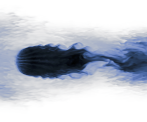
Next, we will examine how the kelp forest and flow interact. Figure 5 shows a kelp forest with  $1$ kelp individual m $^{-2}$, the flow is illustrated by the tracer released from the forest as described above. In column (a) the kelp forest is shown when the background flow speed is maximum, and in column (b) when the background flow speed is minimum (although, as discussed above, this does mean some of the flow will have reversed). In the top row, a region showing the full extent of the tracer advection is shown, and the bottom row shows a zoomed-in region around the kelp forest. In the bottom row, the kelp canopy is also shown as arrows pointing from the position where the individual reaches the surface to the free end.
Visualisation the flow through and around a realistic density (1 individuals m $^{-2}$) kelp forest at peak (a), and minimum (b) background velocity illustrated by the depth-averaged tracer concentration (normalised by the maximum to give saturation).

At the time of maximum speed shown in (a) the flow through the kelp forest is sufficiently attenuated to induce shear instability, causing mixing with water outside the wake. As the flow relaxes in (b) the turbulent wake spreads. Additionally, mixing with external water is caused by flow separation leading to von Kármán vortex street formation downstream of the kelp forest. This is not a significant source of mixing at this density, but is more apparent at higher densities (see figure 7).
During the peak flow phase the advection and mixing are sufficient to prevent the tracer from becoming saturated within the kelp forest, but as the flow relaxes it quickly becomes fully saturated in and around the kelp forest. This leads to regions of high tracer concentration at either end of the tidal cycle as can be seen in the top row of column (b) where the area from the previous flow relaxation can be seen to the right of the kelp forest.
Figure 5 also highlights the deformation of the kelp canopy. In column (a) it can be seen that the canopy on the upstream side of the kelp forest is shifted in the direction of the flow, while the canopy elsewhere is shielded from the background flow and relatively undisturbed. At the time corresponding to minimum flow speed (b), the canopy remains deflected to the right, showing that the canopy position retains some ‘memory’ of the earlier flow.
Figure 6 shows the time- and depth-averaged mean flow in (a,b), and the mean canopy position in (c). The mean flow (a,b) exhibits a pattern similar to a pure strain flow with mean flow into the kelp forest from the left and right ( $x$) and out in the spanwise direction ( $y$). This can be explained through a ‘rectification’ of the tidal flow. When the tidal current is in the $+x$ direction, the speed to the left (upstream) of the kelp forest is larger than the speed to the right (downstream) of the kelp forest due to drag on the flow through the kelp forest. Similarly, when the tidal current is in the $-x$ direction, the speed is larger on the right of the kelp forest. As a result, the Eulerian time-mean flow to the left and right of the kelp forest is inward, and the mean flow must then exit the kelp forest in the $\pm y$ direction to conserve volume. The mean flow is reflected in the mean canopy position.
Time- and depth-averaged mean flow (a) and a zoom of the kelp forest region (b). The time-averaged position of the kelp forest canopy (c). The arrows in (c) point from the location where the kelp first reaches the surface to the end of the kelp.

Finally, we should note that some channelling behaviour is seen within the kelp forest, most notably in figure 6(a,b), where a jet of higher mean flow is seen in the centre of the kelp forest. The kelp position seen in figure 5 suggests that this is due to the kelp arranging themselves in such a way that there are several lower resistance channels through the kelp forest. It is unclear if this effect happens in reality, and may be due to the regular positioning of the individuals and symmetry in the kelp forest geometry in our set-up, as well as the finite resolution with which the flow is resolved.
3.3 Influence of kelp forest density on tracer release, advection and mixing
Figure 7 shows the tracer distribution in simulations with different kelp forest densities. At the lowest density, in (a), the tracer is distributed almost completely along the line that passes through the kelp forest as very little turbulent mixing occurs, and the tracer is not saturated at any point in the tidal cycle. At intermediate densities, mixing between high and low tracer water is enhanced by shear instabilities at the edge of the wake (figures 7(b) and 5). At higher densities, mixing is further enhanced as a von Kármán vortex street develops in the wake (c,d). At very high densities (d) the tracer is fully saturated inside the kelp forest and drag reduces the rate of exchange of water inside and outside the kelp forest. This effect will be explored below.
Examples of the final tracer distribution in models of an idealised kelp forest of varying density. At higher densities the flow experiences turbulent breakdown, significantly increasing the volume of water mixed through the forest.

In order to quantify the tracer release and the rate of mixing between waters inside and outside the kelp forest, figure 8(a) shows the tracer concentration expressed as a percentage of the saturation value, averaged across the whole domain ( $\times$), and within the kelp forest ( $+$). The mean tracer concentration in the full domain reaches a maximum at ${\sim }1.5$ individuals m $^{-2}$ and decreases slowly for higher densities. In contrast, the tracer concentration inside the kelp forest increases monotonically, but the rate of increase slows at high densities as the tracer concentration approaches the saturation value. As a result, the ratio of the tracer concentration inside and outside the kelp forest reaches a distinct minimum at a density of ${\sim }1.5$ individuals m $^{-2}$. One explanation for this is that, for densities larger than 1.5 individuals m $^{-2}$, the total tracer release is limited by the exposure of low saturation water to the kelp forest.
(a) The time-averaged tracer concentration (as a percentage of the fully saturated value) averaged over the full computational domain ( $\times$) and averaged within the kelp forest ( $+$) as a function of kelp forest density. (b) The ratio between the mean tracer concentration inside the kelp forest and within the full domain. Note the different vertical scales used for the whole domain (a) and inside the forest (b).

To test this hypothesis, we can estimate the time scales involved in the volume-averaged tracer evolution equation
 \begin{equation} \frac{1}{V}\int\frac{\partial C}{\partial t}{\rm d} V = \frac{\partial \bar{C}}{\partial t} = {-}\frac{1}{V}\int\boldsymbol{u} \boldsymbol{\cdot}\boldsymbol{\nabla} C \,{\rm d} V + \frac{\varSigma}{\tau}(C_0-\bar{C}). \end{equation}
In the absence of advection, the tracer release term (the second term on the right-hand side) dominates, and we can find the release time scale
 \begin{equation} \tau_r = {-}\frac{\tau}{\varSigma}\ln0.1. \end{equation}
We can compare this tracer release time scale with a time scale associated with advection. For a kelp forest of radius  $r_f$ and a mean speed within the kelp forest $|\bar {u}|$, the time for a fluid parcel to move from the middle to the edge of the forest is
 \begin{equation} \tau_{adv} = \frac{r_f}{|\bar{u}|}. \end{equation}
It is also useful to form a length scale characterising the distance that a fluid parcel would travel inside the kelp forest before reaching 90 % saturation
 \begin{equation} \ell \equiv |\bar{u}|\tau_r = {-}|\bar{u}|\frac{\tau}{\varSigma}\ln0.1. \end{equation}
 Figure 9 shows these scales as a function of the kelp forest density, where  $|\bar {u}|$ is diagnosed from the simulations by averaging the velocity inside the kelp forest. Note that both time scales are significantly shorter than the tidal period (12.4 h), and hence we assume that the tidal period does not play a major role in limiting the tracer release. As expected, the release time scale ( $\times$) decreases like $1/\varSigma$ as there are more kelp individuals releasing tracer for high densities. The advection time scale ( $+$) linearly increases with density, indicating the reduction in flow speed by drag at high densities. The release and advection time scales intersect at a density of ${\sim }1.5$ individuals m $^{-2}$. This suggests that the maximum in the whole domain tracer concentration (figure 7a) can be explained by the limiting time scales. At the density where $\tau _r=\tau _{adv}$, the rate of tracer release matches the rate at which water inside the kelp forest is replaced by water from outside the kelp forest. At lower densities, $\tau _{adv} < \tau _r$, and thus the water parcels do not remain within the kelp forest long enough for the tracer to become fully saturated. At higher densities, $\tau _r < \tau _{adv}$ and thus the water inside the kelp forest becomes fully saturated before it has time to exit the kelp forest.
Release and advection time scales for varying density kelp forests intersecting at the density of maximum tracer release, along with the saturation-scale length which corresponds to the kelp forest radius at the density of maximum tracer release.

Another way of viewing this is through the saturation length scale ( $\ell$), which decreases with density. At the density of maximum tracer release, $\ell$ corresponds to the kelp forest radius (100 m, indicated by a horizontal line), suggesting that at high densities the water cannot be advected out of the kelp forest before it is saturated.
We also estimated the turbulent mixing time scale between the wake and surrounding water
 \begin{equation} \tau_{mix} = \frac{r_f}{v'}, \end{equation}
where  $v'$ is a fluctuating (turbulent) velocity which we took to be the spanwise root-mean-square velocity, and $r_f$ is the kelp forest radius. The mixing time scale is $5$ times (for the highest densities) and $10$ times (for the lowest densities) larger than the advection time scale. This suggests that horizontal mixing between the wake and ambient flow does not play a large role in setting the rate of tracer release over the time scale considered, and also explains why the tracer concentration outside of the wake increases slowly (as seen in e.g. figure 10). In reality, we anticipate that a non-zero mean flow would advect water containing the tracer out of the path of the tidal oscillation, but our idealised simulations do not include this effect.
Panel (a) shows the background tidal speed (grey), and mean speed within the kelp forest (blue). Panel (b) shows the evolution of the mean tracer saturation in the along-shore direction and time. The black dashed lines show the extent of the kelp forest, and the grey lines the theoretical tidal excursion extent. The white contour shows the 90 % isosaturation.

This leaves the question of how far the tracer-containing water travels from the kelp forest in our simulations. Figure 10(a) shows the mean speed inside the kelp forest (blue) compared with the ambient tidal flow (grey) and (b) shows a time series of the tracer concentration (in units of % saturation) as a function of streamwise distance at  $y=0$ for a density of 1.5 individuals m $^{-2}$. For reference, the tidal excursion length for the ambient flow is indicated in dashed lines in (b) and a white contour shows the tracer saturation of 90 %. During phases of peak flow speed, the upstream side of the 90 % saturation contour reaches the centre of the kelp forest, consistent with the length and time scale analysis above. In the downstream direction, the 90 % saturation contour extends about 500 m from the centre of the kelp forest. This is significantly smaller than the ambient tidal excursion length and reflects the reduced flow speed inside and downstream of the kelp forest. However, water with lower tracer concentrations is mixed into the high-speed regions surrounding the kelp forest and reaches or slightly exceeds the ambient excursion length.
4. Discussion and conclusions
In this study, we incorporated a dynamical model of giant kelp motion within a LES to simulate flow interactions with an idealised kelp forest. We used a simplified tracer released from the kelp individuals to understand how the flow interactions and variations in the kelp forest density may limit nutrient uptake and the transport of dissolved substances. We calibrated the model using an EKI to quantitatively match field measurements and then conducted a series of controlled experiments where the density of kelp within the forest was varied.
Our model showed a good quantitative fit to the field measurements from Reference GaylordGaylord et al. (2007) and replicated key flow features observed in the field. In particular, the ratio of the velocity measured at fixed locations inside and outside the kelp forest fell largely within the uncertainty in the field observations. Our model also replicated the key observed flow features: a lack of a stable recirculation zone downstream of the kelp forest (even for higher kelp forest densities) and a low-speed wake downstream of the forest. The Eulerian time-averaged velocity exhibited tidal rectification, where the slower flow in the lee of the kelp forest led to a convergent time-mean flow in the direction of the tidal currents.
The qualitative flow structures seen in our simulations depend on the kelp forest density. At very low densities ( ${<}0.5$ individuals m $^{-2}$) the flow is relatively unimpeded by the kelp forest and the flow remains largely unidirectional. At intermediate densities that are typical of natural kelp forests, horizontal shear instabilities develop at the border between a low-speed wake in the lee of the kelp forest and the faster ambient water. The resulting turbulence mixes water that was in contact with the kelp forest with the ambient water. At higher kelp densities, flow separation occurs and a von Kármán vortex street forms in the wake of the kelp forest. Due to the floating canopy, the surface velocity is slowed more than the depth-averaged velocity, consistent with previous laboratory experiments (Reference Rosman, Denny, Zeller, Monismith and KoseffRosman et al. 2013).
Our simulations included a dissolved tracer which was released by the kelp. The release rate was chosen to be a simple function of the ambient tracer concentration and the kelp density so that the release rate approaches zero as the ambient tracer concentration approaches a saturating concentration. This was intended to mimic the release of tracers such as dissolved organic carbon or oxygen or the update of tracers such as nitrate and phosphate.
Interestingly, we found that the total tracer released by the kelp reaches a maximum at a density of approximately 1.5 individuals m $^{-2}$. A time scale analysis reveals that, for smaller densities, the time scale associated with tracer release is slower than the advection time and the total tracer increases with increasing density. For densities larger than 1.5 individuals m $^{-2}$, where drag significantly slows the flow through the kelp forest, the advection time scale is slower than the tracer release. As a result, the tracer within the kelp forest becomes saturated and the exchange between this saturated water and the ambient water is limited, thus reducing the total amount of tracer released.
Our results suggest that the density of maximum tracer release corresponds roughly with the density of natural kelp forests of comparable size. This may suggest that the density of natural kelp forests is limited, in part, by the ability of the kelp forest to uptake more nutrients, although given our model simplifications many other factors such as light limitation need to be considered. Nonetheless, the dependence of the tracer export rate on the kelp density might prove to be an important consideration in the design of kelp farms where the desire is to maximise the growth rate (and uptake of nutrients) and the export of carbon.
Our model captures flow–structure interactions between the tidal currents and turbulence and the deformable kelp individuals. Tidal rectification displaces the time-mean position of the kelp towards the centre of the kelp forest along the axis aligned with the tidal currents. We also found some evidence for small-scale channelling within the kelp forest. The reasons for this effect are unclear and this may be due to the regular spacing of the individuals in the model or the finite numerical resolution.
For kelp forest densities larger than 1.5 individuals m $^{-2}$, the flow of water through the kelp forest is significantly limited by drag from the kelp. As a result, water with the highest tracer concentration does not extend very far from the kelp forest (compared with the ambient tidal excursion length). This has implications for the area that is most impacted by the kelp forest and might need to be considered when planning multiple kelp farms.
Additionally, our results suggest that export from the kelp forest (in particulate and dissolved form) may not be transported far from the kelp forest at higher kelp forest densities due to the reduction in the tidal excursion length within the kelp forest. These results may also be important for consideration when planting artificial kelp forests, for example when ensuring that detritus is transported sufficiently far from the kelp forest to be moved to the slow carbon cycle, or for planning planting density and layout to optimise growth potential. Additionally, our results emphasise the need account for near-field flow features in lower-resolution simulations that are unable to fully resolve these processes.
The simulations presented here are idealised and were designed to identify physical mechanisms involved in the fluid/kelp forest interactions and their influence on tracer exchange. In reality, the kelp forest geometry, bathymetry and other factors which may influence the flow/kelp interactions will influence the tracer exchange rates. The release or uptake rates for biologically active tracers such as carbon or nutrients will depend on the complicated biology involved in kelp growth and ecosystem dynamics. Important next steps for future work include coupling the coupled kelp/flow model with a biogeochemical model, implementing an active kelp growth model and exploring a more realistic kelp forest geometry.
Supplementary material
Supplementary movie is available at https://doi.org/10.1017/flo.2024.13. The code for the giant kelp model and coupling, calibration and density variation experiment are available at https://github.com/jagoosw/GiantKelpDynamics where they are provided as a Julia package and scripts. An archive of the code version used for the experiments can be found at Reference Strong-Wright, Chen, Constantinou, Silvestri, Wagner and TaylorStrong-Wright (2024). The experiment outputs are available upon request from the authors.
Acknowledgements
We would like to thank the CliMA team (https://clima.caltech.edu/) and other Oceananigans.jl (Reference Ramadhan, Wagner, Hill, Jean-Michel, Churavy, Souza, Edelman, Ferrari and MarshallRamadhan et al. 2020) contributors for making our simulations much easier, contributors to EnsembleKalmanProcesses.jl (Reference Dunbar, Lopez-Gomez, Garbuno-Iñigo, Huang, Bach and WuDunbar et al. 2022) for their fantastic tool which facilitated our model calibration and Makie.jl (Reference Danisch and KrumbiegelDanisch & Krumbiegel 2021) contributors for making the figures possible. The authors are grateful to the Climate Foundation and the Kelp Forest Foundation for many helpful discussions.
Funding
J.S.W. was supported by the Centre for Climate Repair, Cambridge (https://www.climaterepair.cam.ac.uk/). J.R.T. was supported by a grant from the Gordon and Betty Moore Foundation, facilitated by the Kelp Forest Foundation.
Declaration of interests
The authors report no conflict of interest.
Author contributions
J.S.W. ran and analysed the simulations with support from J.R.T. Both authors designed the study and wrote the paper.
Appendix A. Calibration
As described in § 2.2.1 we calibrated three model parameters: the blade drag coefficient,  $C_{DB}$, the forest dropoff factor, $d$, and the tidal amplitude $A_u$. Statistics from the observations reported in Reference GaylordGaylord et al. (2007) are shown in table 2. The flow amplitudes $\sigma _u$ at each station provide information about the tidal speed, and the velocity ratios (relative to the reference station) for stations $4$ and $8$ provide information about the reduction in current speed due to the forest.
Measurables for parameter calibration, reproduced from Reference GaylordGaylord et al. (2007).

The values listed in table 2 were used as the observations to use for parameter estimation. Using the ensemble Kalman process package from Reference Iglesias, Law and StuartIglesias et al. (2013) with 12 ensemble members, we estimated the amplitude of the three parameters that produced the best fit to the statistics given in table 2.
The results of the calibration are shown in table 3, which gives the optimised parameter values, the minimum and maximum value in the final ensemble and the standard deviation. Figure 11 shows the velocity ratios between station  $4$ and $1$ in the final ensemble for the last tidal cycle. The scattered points indicate the velocity at each station from the LES at a single time, and the solid black line is the best fit applied to the positive and negative velocity values separately. The LES data show a good fit to the observations reported in Reference GaylordGaylord et al. (2007), shown as a grey line. The majority of model points lie within the standard deviation of the observations (the grey shaded region), with a few lying outside, most likely due to the details of the forest geometry and forcing.
The EKI optimised parameter values and ranges.

Ratio of along-shore velocity at points inside and outside of the kelp forest at locations similar to those reported in Reference GaylordGaylord et al. (2007). The negative quadrant (‘downstream’) relationship has a gradient of  $0.29$ and the positive quadrant (‘upstream’) has a gradient of $0.51$. The relationship and 95 % confidence intervals from Reference GaylordGaylord et al. (2007) are shown with the grey solid line and the shaded grey region for comparison. The grey dashed line shows the 1:1 ratio for reference.

Appendix B. Comparison with the Reference Rosman, Denny, Zeller, Monismith and KoseffRosman et al. (2013) laboratory experiment
To compare our results with the laboratory experiment of Reference Rosman, Denny, Zeller, Monismith and KoseffRosman et al. (2013) we replicated their model with the parameters (i.e. density and flow speed) of the observed forest their scaled model was based on. We used a  $y$- and $z$-bounded, $x$-periodic, domain $1\,{\rm km} \times 250\,{\rm m}\times 8$ m with $256$ points km $^{-1}$ in the horizontal and $1$ point metre $^{-1}$ in the vertical. The first $100$ m of the domain was filled with kelp with a density of $0.65$ individuals m $^{-2}$ each with two nodes 8 m long. In the second half of the domain, the velocity was restored to 0.1 m s $^{-1}$ (so the ‘inflow’ at the edge of the forest was uniform and 0.1 m s $^{-1}$). In all other regards the model was configured the same as the other experiments. We ran the model for 10 h, during which time it equilibrated. Figure 12 shows the average velocity in the central half of the domain within the forest which closely matches the data from Reference Rosman, Denny, Zeller, Monismith and KoseffRosman et al. (2013).
Comparison of the depth profile of water speed in a uniform forest configured to replicate the laboratory experiment of Reference Rosman, Denny, Zeller, Monismith and KoseffRosman et al. (2013) showing a good match. The blue line shows the velocity profile from our model and the black  $\times$ show data reproduced from Reference Rosman, Denny, Zeller, Monismith and KoseffRosman et al. (2013). Although not shown here, our model everywhere lies within the error bars of the original data.

Appendix C. Grid resolution sensitivity
To ensure that the grid resolution  $256\times 256$ gridpoints per kilometre was sufficient, we did a grid sensitivity test by using $128\times 128$, $256\times 256$ and $512\times 512$ gridpoints per kilometre. These runs were conducted with a reduced domain size ( $3\,{\rm km}\times 1\,{\rm km}$) and a kelp density of $0.5$ individuals m $^{-2}$ to reduce computational cost.
Figure 13 shows snapshots of the tracer concentration after one full tidal cycle. The tracer saturation is qualitatively similar in all three simulations, although the tracer field appears somewhat ‘blurred’ in the lowest resolution case since the smallest-scale motions are not resolved.
The depth-averaged tracer saturation after one tidal cycle for three different horizontal resolutions.

We also calculated the mean tracer saturation across both the full domain and within the forest (in the same way as presented in figure 8). These are shown in table 4 and quantify the differences observed above. The tracer saturation both inside and outside the forest is very similar in all three cases.
Tracer saturation at different grid resolutions. Fractional changes relative to the  $512\times 512$ values.

This resolution sensitivity test gives us confidence that the resolution of  $256$ gridpoints per kilometre that we used in the simulations presented in the main text is sufficient to capture the fine-scale motions seen in the higher resolution simulation, while adequately reproducing the tracer statistics.
Appendix D. Dynamics model parameter sensitivity
While there are a large number of parameters in the kelp dynamics model ( ${\sim }10$), the majority of these have been directly measured in M. pyrifera in previous work. For example, we use the mean blade areas and distribution from Reference Jackson, James and NorthJackson et al. (1985). On the other hand, there are a few parameters which cannot easily be inferred from the existing literature. The most uncertain parameter (with no previous inference or direct measurement) was the drag coefficient of the kelp blades. We calibrated this as described in § 2.2.1. The other parameters which were not directly measured when configuring previous versions of the Reference Utter and DennyUD96 model are the spring constants. Originally these were inferred by fitting to an unpublished set of observations.
To check that uncertainty in the spring constants is not important for the analysis in this paper we varied the spring constant ( $k$) between $0.5$ and $2$ times the original value. When varying the spring constant across this range, the mean tracer concentration inside the kelp forest changed by less than 0.78 %, while the mean tracer concentration in the full domain changed by less than 0.075 %. These small changes suggest that the spring constant does not have a significant impact on the tracer release rate, which is a key focus of this paper.


 Open access