

1 Introduction
1.1 Study motivation
In the social and behavioral sciences, identifying the predictors that most strongly influence behavioral or performance outcomes is one of the central objectives of empirical research. Researchers frequently seek to understand how individual characteristics (e.g., demographic information), cluster-level factors (e.g., school environment and classroom composition), and item-specific attributes (e.g., item format or task type) contribute to outcomes scored as binary variables, such as correct versus incorrect responses. Identifying and prioritizing key predictors is critical not only for enhancing explanatory and predictive accuracy but also for generating interpretable insights that advance theory and practice. Achieving this requires partitioning the systematic effects of predictors from random variation at the group levels (individual, cluster, and item) in order to more accurately estimate their explanatory power.
The current study is developed within the framework of explanatory item response models (EIRMs; De Boeck & Wilson, Reference De Boeck and Wilson2004) and multilevel item response models (MIRMs; Fox, Reference Fox2010), a class of psychometric models formulated as generalized linear mixed-effects models (GLMMs; McCulloch et al., Reference McCulloch, Searle and Neuhaus2008) for item response data. In this psychometric context, item responses are modeled at the item level while simultaneously accommodating person-, item-, and context-level predictors, thereby linking measurement to substantive explanation. Fixed effects represent the systematic influence of predictors, such as individual, cluster, or item characteristics. Random effects, in turn, capture variations specific to individuals, clusters, or items, such as differences between schools, students within schools, or test items.
The methodological contribution is therefore intended to support psychometric goals that extend beyond score estimation, namely, explaining systematic variation in item responses and latent-trait-related performance using theoretically meaningful predictors and contextual information. For example, in educational measurement, this framework helps investigate whether student-level attributes, such as prior knowledge or engagement, outweigh school-level influences, thereby guiding the design of personalized interventions. In health-related measurement, this approach can illustrate how patient-reported outcome items can be analyzed by incorporating patient characteristics, provider-level contextual predictors, and item-level content features. This supports the explanatory modeling of symptom severity by, for example, identifying which specific patient risk factors (e.g., age or smoking status), provider characteristics (e.g., facility size), or item domains (e.g., emotional vs. physical symptoms) are most strongly associated with reported severity, while disentangling individual-level variability from between-provider heterogeneity. A method that preserves both explanatory and predictive accuracy while maintaining interpretability across levels of analysis is therefore essential for making valid interpretations and data-driven decisions in these domains.
However, several methodological challenges arise when applying GLMMs, EIRMs, or MIRMs to identify important predictors. First, integrating numerous predictors is difficult due to both the scale of the data and its incompatibility with these models. For example, modeling 20 predictors already requires estimating 20 main effects; adding every two-way interaction and each predictor’s quadratic term raises the total to 230 effects. This level of complexity quickly exceeds the practical limits of GLMMs, EIRMs, or MIRMs—especially in the presence of modest sample sizes or sparse response data. Second, the relationships between predictors and item responses may follow diverse, non-linear patterns that are not easily captured by linear modeling assumptions. Moreover, interactions between individual-, cluster-, and item-level predictors may involve complex, higher-order dependencies that are difficult to specify a priori. Third, identifying the most relevant predictors while avoiding overfitting is critical when there are many predictors. Addressing these challenges is necessary to ensure that these models provide robust and interpretable measurement and prediction of behavior and performance.
1.2 Related methods and current limitations
GLMMs, EIRMs, or MIRMs effectively capture variations specific to individuals, clusters, or items, providing interpretable estimates of fixed and random effects, and statistical inference on the estimates. However, these models typically assume linear relationships between predictors and outcomes, and any potential nonlinearities—such as quadratic terms, splines, or interactions—must be specified manually. This requirement limits their flexibility and may result in oversimplified models that fail to capture complex, nonlinear dependencies often present in social and behavioral data, potentially overlooking important predictive patterns.
On the other hand, machine learning (ML) methods such as ensemble approaches that leverage multiple models—such as random forests (Breiman, Reference Breiman2001) and extreme gradient boosting (XGBoost; Chen & Guestrin, Reference Chen and Guestrin2016)—are designed to model complex, non-linear relationships and interactions among predictors, making them powerful tools for predictive tasks. However, when applied to multilevel binary item response data without accounting for hierarchical structure, these ML methods are expected to misattribute individual-, cluster-, or item-level variation to observed predictors. For example, in educational testing, item-level differences (e.g., basic arithmetic vs. multi-step word problems in a math test) may be incorrectly attributed to individual student characteristics, inflating their apparent predictive importance and leading to misleading interpretations. This conflation of fixed and random effects reduces model interpretability and can compromise explanatory and predictive accuracy in contexts with substantial multilevel heterogeneity.
To overcome the limitations of traditional parametric models while leveraging the flexibility of ML, combining GLMMs with simpler ML techniques or using ensemble methods has been explored.Footnote 1 The general idea of these hybrid approaches is to replace the fixed-effect component in a GLMM with an ML method while retaining random effects to account for multilevel structures. Fokkema et al. (Reference Fokkema, Edbrooke-Childs and Wolpert2021), Lin and Luo (Reference Lin and Luo2019), and Speiser et al. (Reference Speiser, Wolf, Chung, Karvellas, Koch and Durkalski2020) replaced the fixed-effect component with a decision tree (Breiman et al., Reference Breiman, Friedman, Olshen and Stone1984) for longitudinal or multilevel binary outcomes. In addition, Speiser et al. (Reference Speiser, Wolf, Chung, Karvellas, Koch and Durkalski2019) and Pellagatti et al. (Reference Pellagatti, Masci, Ieva and Paganoni2021) used random forests, and Ngufor et al. (Reference Ngufor, Van Houten, Caffo, Shah and McCoy2019) employed random forests, gradient boosting machine, model-based recursive partitioning, and conditional inference trees for longitudinal binary outcomes (persons nested within multiple time points) in a GLMM. Similarly, Cho et al. (Reference Cho, Goodwin, Salas and Mueller2025) applied a GLMM-random forests approach to single-level cross-classified item response data, adapting the algorithm from Speiser et al. (Reference Speiser, Wolf, Chung, Karvellas, Koch and Durkalski2019) with modifications. Speiser et al. (Reference Speiser, Wolf, Chung, Karvellas, Koch and Durkalski2019, Reference Speiser, Wolf, Chung, Karvellas, Koch and Durkalski2020) and Cho et al. (Reference Cho, Goodwin, Salas and Mueller2025) treat predicted probabilities from the ML method (decision tree or random forests) as a slope of a known predictor in the GLMM and iteratively update the binary response variable using a combination of observed and predicted outcomes until convergence. These algorithms have performed well for prediction or explanation in longitudinal binary outcomes and single-level cross-classified data, as demonstrated in their respective studies. Estimating the slope of the predicted probabilities as a predictor is a flexible approach to estimate the predictive power of the ML-based values.
However, the algorithms in the prior approaches may not always be effective due to several limitations. First, in Cho et al. (Reference Cho, Goodwin, Salas and Mueller2025) and Speiser et al. (Reference Speiser, Wolf, Chung, Karvellas, Koch and Durkalski2019, Reference Speiser, Wolf, Chung, Karvellas, Koch and Durkalski2020), by estimating a slope for the ML-based predictions, these methods treat the ML output as a predictor whose influence is adjusted within the GLMM. Although this strategy captures the association between the predictions and the outcome, it does not explicitly separate the ML component (capturing non-linear and interactive fixed effects) from the GLMM’s role (modeling random effects as deviations from the fixed effects).
Second, updating the observed outcome with the predicted probabilities in Cho et al. (Reference Cho, Goodwin, Salas and Mueller2025) and Speiser et al. (Reference Speiser, Wolf, Chung, Karvellas, Koch and Durkalski2019, Reference Speiser, Wolf, Chung, Karvellas, Koch and Durkalski2020) produces a hybrid outcome that deviates from the original data, potentially reducing interpretability by obscuring the direct relationship between predictors and true outcomes—which is critical in applied fields like education and psychology. Unlike Cho et al. (Reference Cho, Goodwin, Salas and Mueller2025) and Speiser et al. (Reference Speiser, Wolf, Chung, Karvellas, Koch and Durkalski2019, Reference Speiser, Wolf, Chung, Karvellas, Koch and Durkalski2020), Pellagatti et al. (Reference Pellagatti, Masci, Ieva and Paganoni2021) used raw residuals (also known as response residuals), defined as the difference between the observed outcome and the prediction from the random forests, to isolate ML predictions in the GLMM and to update the outcome over iterations in the algorithm. However, raw residuals for binary data are limited in utility because their discrete nature and heteroscedasticity make them less informative for diagnosing model fit or identifying patterns in GLMMs. Ngufor et al. (Reference Ngufor, Van Houten, Caffo, Shah and McCoy2019) proposed an iterative framework to combine ML and GLMM. At every iteration, they construct a “modified outcome” or working response by adding the current linear predictor to a variance-scaled residual and subtracting the current empirical-Bayes predictions of the random effects. The authors then train an ML on this adjusted outcome. From the ML’s output, they created indicator variables—new binary features that represent the complex, non-linear relationships and regions identified by the model—which are then added to the next GLMM iteration as fixed-effect predictors. This approach is subject to potential “iteration-lag” overlap, which may introduce redundancy and numerical instability. That is, indicators learned at iteration t are incorporated at iteration $t+1$
, and the intervening updates to the working response and random-effects predictions can render those indicators stale or partially collinear.
$t+1$
, and the intervening updates to the working response and random-effects predictions can render those indicators stale or partially collinear.
Third, when predictors are defined at any group level (e.g., person, cluster, or item), the failure to separate systematic group-level effects from random variation can cause this random variation (such as differences between individuals, schools, or items) to be absorbed into the predicted probabilities. This misallocation can bias importance measures from ML by overemphasizing group-level factors—such as socioeconomic status in educational data—and reduce the model’s ability to accurately distinguish between fixed and random effects in multilevel settings. However, previous approaches have not addressed how to properly isolate the effects of group-level predictors from random effects within the GLMM–ML framework.
The importance measure, such as a permutation importance measure, has been used to identify important predictors from ML (e.g., Jacobucci et al., Reference Jacobucci, Grimm and Zhang2023). However, in multilevel binary data with grouping structures at the person, cluster, and item levels, applying a regular permutation importance measure introduces important limitations. Standard row-wise permutation breaks the natural dependency structure by shuffling predictor values across all observations, regardless of their grouping. This can generate implausible data configurations (e.g., assigning different cluster-level values to individuals within the same cluster), distorting the contributions of predictors. To address analogous issues in neuroimaging, Winkler et al. (Reference Winkler, Webster, Vidaurre, Nichols and Smith2015) developed a multi-level block permutation framework for using general linear models, which restricts permutations to subsets that respect hierarchical exchangeability. By treating observations or entire blocks as weakly exchangeable and nesting them hierarchically, their approach preserves the joint dependence structure and yields valid inference for repeated-measures, family-based, or longitudinal designs. In the context of GLMMs, random intercepts can account for within-cluster dependency, but permutation tests still need to be aligned with the level of the predictor being tested: individual-level predictors should be permuted within clusters, whereas cluster-level predictors should be permuted at the cluster level. This ensures that permutation schemes remain consistent with the hierarchical data structure and avoids generating implausible data configurations. However, to our best knowledge, a permutation importance measure that fully accounts for multilevel structures has not yet been developed in the applications of ML.
In prior work, Cho et al. (Reference Cho, Goodwin, Salas and Mueller2025) employed random forests to enhance prediction accuracy for single-level cross-classified item response data beyond what is achievable with a single GLMM. In the current study, XGBoost is particularly well aligned with the iterative algorithm to be developed, as it updates residuals to capture complex relationships among predictors, facilitating the refinement of fixed and random effects alongside the GLMM’s modeling of multilevel structures. Yet the implementation of GLMM–XGBoost has not been demonstrated for multilevel binary item response data.
1.3 Study purpose and novel contributions
The purpose of this study is to develop, apply, and evaluate an iterative GLMM–XGBoost algorithm for analyzing multilevel binary item response data, directly addressing the limitations of existing hybrid approaches. The algorithm’s novelty lies in replacing the penalized weighted least squares step in the penalized IRLS (PIRLS) routine with a more flexible XGBoost learner. In addition, a weighted orthogonal projection is implemented to correctly disentangle the flexible XGBoost learner from random effects in the multilevel binary item response data. Furthermore, results from the iterative GLMM–XGBoost yield variable-importance measures, termed group-aware conditional permutation importance, by incorporating group-aware permutations and conditioning on random effects. This approach is critical for identifying predictors influencing outcomes in the presence of non-negligible random variation. In addition, an uncertainty measure for the group-aware conditional permutation importance is provided. An iterative GLMM–XGBoost algorithm and a group-aware conditional permutation importance measure are illustrated using an empirical dataset and are compared with standalone XGBoost. In addition, simulation studies are conducted to assess the feasibility of the iterative GLMM–XGBoost algorithm across a range of multilevel designs and tree structures, and to evaluate its performance relative to XGBoost, GLMMs, generalized additive mixed models (GAMMs; Wood, Reference Wood2017), and GLMM-tree models. An accompanying R function that automates the iterative GLMM–XGBoost algorithm is publicly available on the Open Science Framework (OSF) at https://osf.io/knmyh/overview.
To clarify the conceptual gap addressed by the proposed approach, it is useful to contrast standard GLMMs, standalone XGBoost, and the iterative GLMM–XGBoost framework developed in this study in terms of (a) how fixed effects are updated, (b) how random effects are treated, and (c) how predictor importance is interpreted. In a standard GLMM, fixed effects are updated through parametric optimization (e.g., PIRLS), requiring pre-specification of functional forms and interactions, while random effects explicitly capture unobserved heterogeneity at the person, cluster, or item levels. Accordingly, predictors are interpreted primarily through model coefficients (and associated inferential summaries), with complex nonlinearities or high-order interactions accommodated only when explicitly specified. In contrast, standalone XGBoost flexibly captures nonlinearities and high-order interactions through recursive tree-based learning, and predictor importance is typically summarized using model-based importance measures (e.g., gain- or permutation-based indices); however, because hierarchical dependence is ignored, fixed and random sources of variation can be conflated, potentially biasing importance assessments in multilevel data. The proposed iterative GLMM–XGBoost framework bridges these approaches by replacing the parametric fixed-effect update within the GLMM fitting algorithm with an XGBoost learner, while retaining random effects to model structured dependence. This integration preserves the separation between systematic fixed effects and random variation and yields predictor-importance summaries via group-aware, conditional permutation schemes that remain interpretable under multilevel structure.
The current study focuses on a data-driven, exploratory approach to modeling complex relationships without the need for a priori specification of interaction and polynomial terms. By reliably identifying the relevant predictors using group-aware conditional permutation importance, the GLMM–XGBoost framework acts as a tool that can help formulate and refine theory by objectively highlighting the most consequential drivers of systematic variation in the outcome.
This article is organized as follows. Section 2 introduces the model and the accompanying iterative GLMM–XGBoost algorithm. Section 3 illustrates their use with an empirical dataset. Section 4 reports a simulation study that evaluates the algorithm, and Section 5 concludes with a summary and discussion.
2 Method
2.1 Model specification
In the model below, the triplet $(p,c,i)$
indexes a single binary response: person p, who belongs to cluster c, answers item i. The binary variable
$(p,c,i)$
indexes a single binary response: person p, who belongs to cluster c, answers item i. The binary variable $y_{pci}$
follows a Bernoulli distribution with success probability
$y_{pci}$
follows a Bernoulli distribution with success probability $\operatorname {logit}^{-1}(\eta _{pci})$
, and
$\operatorname {logit}^{-1}(\eta _{pci})$
, and $\mathbf {x}$
denotes the associated predictor matrix (which may include person-, cluster-, or item-level predictors). The linear predictor
$\mathbf {x}$
denotes the associated predictor matrix (which may include person-, cluster-, or item-level predictors). The linear predictor $\eta _{pci}$
is on the logit scale and is given by
$\eta _{pci}$
is on the logit scale and is given by
 $$ \begin{align} \eta_{pci} = \beta_0 + f(\mathbf{x}) + \alpha_{c} + \theta_{p(c)} + \delta_{i}, \qquad y_{pci} \sim \text{Bernoulli}\!\left(\operatorname{logit}^{-1}\!(\eta_{pci})\right). \end{align} $$
Here, $\beta _0$
is the fixed intercept, and
$\beta _0$
is the fixed intercept, and $f(\mathbf {x})$
is an unknown function of the predictors
$f(\mathbf {x})$
is an unknown function of the predictors $\mathbf {x}$
, estimated via an XGBoost. The terms
$\mathbf {x}$
, estimated via an XGBoost. The terms $\alpha _c$
,
$\alpha _c$
, $\theta _{p(c)}$
, and
$\theta _{p(c)}$
, and $\delta _i$
are random intercepts for the cluster (e.g., school), the person nested within that cluster (often interpreted as a latent variable), and the item (often interpreted as negative difficulty), respectively. These random effects are assumed mutually independent:
$\delta _i$
are random intercepts for the cluster (e.g., school), the person nested within that cluster (often interpreted as a latent variable), and the item (often interpreted as negative difficulty), respectively. These random effects are assumed mutually independent: $\alpha _c \sim \mathcal {N}(0,\sigma _{\alpha }^2)$
,
$\alpha _c \sim \mathcal {N}(0,\sigma _{\alpha }^2)$
, $\theta _{p(c)} \sim \mathcal {N}(0,\sigma _{\theta }^2)$
, and
$\theta _{p(c)} \sim \mathcal {N}(0,\sigma _{\theta }^2)$
, and $\delta _i \sim \mathcal {N}(0,\sigma _{\delta }^2)$
(e.g., Fox, Reference Fox2010). The model for the proposed algorithm, as presented in Equation (1), includes random intercepts only for persons, clusters, and items under the modeling assumption that systematic predictor-related variability including linear, nonlinear, and interaction effects is captured by the flexible fixed component
$\delta _i \sim \mathcal {N}(0,\sigma _{\delta }^2)$
(e.g., Fox, Reference Fox2010). The model for the proposed algorithm, as presented in Equation (1), includes random intercepts only for persons, clusters, and items under the modeling assumption that systematic predictor-related variability including linear, nonlinear, and interaction effects is captured by the flexible fixed component $f(\mathbf {x})$
. Random slopes, which represent systematic variation in the linear effects of lower-level predictors across higher-level units (e.g., clusters), are therefore not included by default.
$f(\mathbf {x})$
. Random slopes, which represent systematic variation in the linear effects of lower-level predictors across higher-level units (e.g., clusters), are therefore not included by default.
XGBoost, developed by Chen and Guestrin, (Reference Chen and Guestrin2016), is an optimized distributed gradient boosting framework. It is used to estimate an unknown function $f(\mathbf {x})$
, capturing potentially nonlinear and high-order interactions among the predictors. XGBoost builds upon the gradient boosting framework originally introduced by Friedman (Reference Friedman2001), which constructs an additive ensemble of decision trees in a forward stage-wise manner. At each iteration m, a new tree
$f(\mathbf {x})$
, capturing potentially nonlinear and high-order interactions among the predictors. XGBoost builds upon the gradient boosting framework originally introduced by Friedman (Reference Friedman2001), which constructs an additive ensemble of decision trees in a forward stage-wise manner. At each iteration m, a new tree $f_m(\mathbf {x})$
is added to the model to correct the errors of the previous ensemble. The prediction at iteration M is the sum of the outputs of all trees:
$f_m(\mathbf {x})$
is added to the model to correct the errors of the previous ensemble. The prediction at iteration M is the sum of the outputs of all trees:
 $$ \begin{align} \tilde{y}^{(M)} = \sum_{m=1}^{M} f_m(\mathbf{x}). \end{align} $$
This iterative process continues until convergence or until a stopping criterion is met.
XGBoost fits one tree at a time by minimizing a second-order Taylor approximation of the loss function, with an added regularization term. The objective function at iteration m for the new tree $f_m(\mathbf {x}_n)$
, for observation n (
$f_m(\mathbf {x}_n)$
, for observation n ( $n = 1, \ldots , N$
), is given by
$n = 1, \ldots , N$
), is given by
 $$ \begin{align} \mathcal{L}^{(m)} = \sum_{n=1}^{N} \left[ g_n f_m(\mathbf{x}_n) + \frac{1}{2} h_{n} f_{m}^2(\mathbf{x}_n) \right] + \Omega(f_{m}), \end{align} $$
where $g_n$
and
$g_n$
and $h_n$
are the first- and second-order gradient statistics of the loss function with respect to the previous prediction, and
$h_n$
are the first- and second-order gradient statistics of the loss function with respect to the previous prediction, and $\Omega (f_m)$
is the regularization term for the new tree. Here, n indexes individual observations in the dataset, each uniquely defined by the triplet
$\Omega (f_m)$
is the regularization term for the new tree. Here, n indexes individual observations in the dataset, each uniquely defined by the triplet $(p,c,i)$
. This regularization prevents overfitting and is defined as
$(p,c,i)$
. This regularization prevents overfitting and is defined as
 $$ \begin{align} \Omega(f_m) = \kappa J + \frac{1}{2}\lambda \sum_{j=1}^{J} ||\omega_j||^2, \end{align} $$
where j indexes the leaves (terminal nodes) of the new tree, J is the number of leaves in the tree, $\omega _j$
is the output value of leaf j,
$\omega _j$
is the output value of leaf j, $\kappa $
penalizes the number of leaves (a proxy for the tree’s complexity), and
$\kappa $
penalizes the number of leaves (a proxy for the tree’s complexity), and $\lambda $
is the
$\lambda $
is the $\ell _2$
(ridge) regularization on the leaf values. An
$\ell _2$
(ridge) regularization on the leaf values. An $\ell _1$
(lasso) regularization term,
$\ell _1$
(lasso) regularization term, $\alpha \sum _{j=1}^{J} |\omega _j|$
(where
$\alpha \sum _{j=1}^{J} |\omega _j|$
(where $\alpha $
is the hyperparameter to encourage sparsity of the leaf values by pushing some of them exactly to zero) can be added.
$\alpha $
is the hyperparameter to encourage sparsity of the leaf values by pushing some of them exactly to zero) can be added.
To find the optimal leaf values and structure, the objective function is simplified by grouping the gradient statistics for all data points within each leaf. For a tree with J leaves, the final per-tree objective (up to an additive constant) is
 $$ \begin{align} \tilde{\mathcal{L}} = \sum_{j=1}^{J} \left[ G_j\,\omega_j + \frac{1}{2}\,(H_j+\lambda)\,\omega_j^{2} \right] + \kappa\,J, \end{align} $$
where $G_j$
and
$G_j$
and $H_j$
are the summed first- and second-order gradient statistics, respectively, over all observations in leaf j. This formulation allows XGBoost to efficiently evaluate the quality of a split by calculating the gain from splitting a node into two.
$H_j$
are the summed first- and second-order gradient statistics, respectively, over all observations in leaf j. This formulation allows XGBoost to efficiently evaluate the quality of a split by calculating the gain from splitting a node into two.
Key tuning parameters, including learning rate (eta), maximum tree depth (max depth), minimum child weight (min child weight), regularization penalties (lambda [ $\ell _{2}\ \text {penalty}$
], alpha [
$\ell _{2}\ \text {penalty}$
], alpha [ $\ell _{1}\ \text {penalty}$
]), minimum loss reduction (gamma), subsampling ratios (subsample and colsample bytree), number of boosting rounds (num boost round), and early stopping rounds, are adjusted to optimize predictive accuracy and efficiency in the iterative GLMM–XGBoost framework for multilevel binary item response data.
$\ell _{1}\ \text {penalty}$
]), minimum loss reduction (gamma), subsampling ratios (subsample and colsample bytree), number of boosting rounds (num boost round), and early stopping rounds, are adjusted to optimize predictive accuracy and efficiency in the iterative GLMM–XGBoost framework for multilevel binary item response data.
2.2 Estimation method: EM-like iterative GLMM–XGBoost
This section first outlines two key components of the iterative GLMM–XGBoost algorithm and then presents the full algorithm. The complete workflow is summarized in Algorithm 1. In addition, the group-aware conditional permutation measure is described in the GLMM–XGBoost based on XGBoost.
2.2.1 Working residuals and precision weights: The IRLS/Newton view
In a standard GLMM, estimation proceeds via PIRLS, which can be viewed as an IRLS/Newton update for the linear predictor augmented with a quadratic penalty induced by the Gaussian random-effects prior. For Bernoulli data with a logit link, the log-likelihood for observation n (indexing individual observations in the dataset, each uniquely defined by the triplet $(p,c,i)$
) is
$(p,c,i)$
) is
 $$ \begin{align} \ell_n(\eta_n) = y_n \eta_n - \log(1 + e^{\eta_n}). \end{align} $$
Let $p_n = \operatorname {logit}^{-1}(\eta _n)$
, where
$p_n = \operatorname {logit}^{-1}(\eta _n)$
, where $\eta _n$
includes both fixed and random effects, and consider linearization around a current estimate
$\eta _n$
includes both fixed and random effects, and consider linearization around a current estimate $\eta _n^{(t)}$
. The score and (negative) Hessian with respect to
$\eta _n^{(t)}$
. The score and (negative) Hessian with respect to $\eta _n$
are
$\eta _n$
are
 $$ \begin{align} U_n = \frac{\partial \ell_n}{\partial \eta_n} = y_n - p_n, \qquad H_n = -\frac{\partial^2 \ell_n}{\partial \eta_n^2} = p_n(1-p_n). \end{align} $$
A single IRLS step for $\eta $
solves a weighted least-squares problem using the working response
$\eta $
solves a weighted least-squares problem using the working response
 $$ \begin{align} z_n^{(t)} = \eta_n^{(t)} + \frac{y_n - p_n^{(t)}}{p_n^{(t)}(1-p_n^{(t)})} \quad \text{with weights} \quad \omega_n^{(t)} = p_n^{(t)}(1-p_n^{(t)}). \end{align} $$
The working response $z_n^{(t)}$
linearizes the log-likelihood around the current estimate
$z_n^{(t)}$
linearizes the log-likelihood around the current estimate $\eta _n^{(t)}$
using the inverse of the Hessian as a scaling factor, which is a standard IRLS technique. The term
$\eta _n^{(t)}$
using the inverse of the Hessian as a scaling factor, which is a standard IRLS technique. The term $\frac {y_n - p_n^{(t)}}{p_n^{(t)}(1-p_n^{(t)})}$
adjusts the residual based on the curvature of the logit function. The weight
$\frac {y_n - p_n^{(t)}}{p_n^{(t)}(1-p_n^{(t)})}$
adjusts the residual based on the curvature of the logit function. The weight $\omega _n^{(t)} = p_n^{(t)}(1-p_n^{(t)})$
is the Fisher information, which correctly reflects the precision of the working response and is consistent with the IRLS framework. This derivation can be linked more directly to the Newton–Raphson method via a Taylor expansion of the log-likelihood around
$\omega _n^{(t)} = p_n^{(t)}(1-p_n^{(t)})$
is the Fisher information, which correctly reflects the precision of the working response and is consistent with the IRLS framework. This derivation can be linked more directly to the Newton–Raphson method via a Taylor expansion of the log-likelihood around $\eta _n^{(t)}$
:
$\eta _n^{(t)}$
:
 $$ \begin{align} \ell_n(\eta_n) \approx \ell_n(\eta_n^{(t)}) + U_n^{(t)}(\eta_n - \eta_n^{(t)}) - \frac{1}{2} H_n^{(t)} (\eta_n - \eta_n^{(t)})^2, \end{align} $$
where $U_n^{(t)} = y_n - p_n^{(t)}$
and
$U_n^{(t)} = y_n - p_n^{(t)}$
and $H_n^{(t)} = p_n^{(t)}(1-p_n^{(t)})$
. Maximizing this quadratic approximation leads to the weighted least-squares update.
$H_n^{(t)} = p_n^{(t)}(1-p_n^{(t)})$
. Maximizing this quadratic approximation leads to the weighted least-squares update.
In matrix form, the IRLS update for fixed effects $\boldsymbol {\beta }$
solves:
$\boldsymbol {\beta }$
solves:
 $$ \begin{align} \mathbf{x}^\top \mathbf{w}^{(t)} \mathbf{x} \Delta \boldsymbol{\beta} = \mathbf{x}^\top \mathbf{w}^{(t)} \mathbf{r}^{(t)}, \end{align} $$
where $\mathbf {x}$
are predictors,
$\mathbf {x}$
are predictors, $\mathbf {w}^{(t)} = \mathrm {diag}(\omega _n^{(t)})$
, and
$\mathbf {w}^{(t)} = \mathrm {diag}(\omega _n^{(t)})$
, and $\mathbf {r}^{(t)}$
are the working residuals. This is exactly a weighted regression of
$\mathbf {r}^{(t)}$
are the working residuals. This is exactly a weighted regression of $\mathbf {r}^{(t)}$
on
$\mathbf {r}^{(t)}$
on $\mathbf {x}$
. Equivalently, regressing the conditional working residuals
$\mathbf {x}$
. Equivalently, regressing the conditional working residuals
 $$ \begin{align} r_n^{(t)} = \frac{y_n - p_n^{(t)}}{p_n^{(t)}(1-p_n^{(t)})} \end{align} $$
on the predictors under the precision weights $\omega _n^{(t)}$
approximates a single IRLS/Newton update for the fixed effects.
$\omega _n^{(t)}$
approximates a single IRLS/Newton update for the fixed effects.
In a standard GLMM, the core update can be viewed as an IRLS/Newton step for the linear predictor, implemented in practice via PIRLS through a penalized WLS sub-problem for $\eta =\mathbf {X}\boldsymbol {\beta }+\mathbf {Z}\mathbf {u}$
. The iterative GLMM–XGBoost algorithm replaces the linear (penalized) WLS sub-problem in this IRLS-type Newton step with a nonlinear tree-boosting sub-problem, while retaining the same local quadratic approximation of the Bernoulli negative log-likelihood. XGBoost is derived from a second-order Taylor expansion of the loss around the current predictor
$\eta =\mathbf {X}\boldsymbol {\beta }+\mathbf {Z}\mathbf {u}$
. The iterative GLMM–XGBoost algorithm replaces the linear (penalized) WLS sub-problem in this IRLS-type Newton step with a nonlinear tree-boosting sub-problem, while retaining the same local quadratic approximation of the Bernoulli negative log-likelihood. XGBoost is derived from a second-order Taylor expansion of the loss around the current predictor $\eta ^{(t)}$
, yielding per-observation first- and second-order statistics. Specifically, for the Bernoulli negative log-likelihood loss
$\eta ^{(t)}$
, yielding per-observation first- and second-order statistics. Specifically, for the Bernoulli negative log-likelihood loss $-\ell _n(\eta _n)$
, the following hold:
$-\ell _n(\eta _n)$
, the following hold:
-
• The second-order curvature statistic used by XGBoost, $h_n^{(t)}$
, is identical to the IRLS precision weight
$\omega _n^{(t)}$
(Fisher information), since
$$ \begin{align*}h_n^{(t)} = \frac{\partial^2}{\partial \eta_n^2}\{-\ell_n(\eta_n)\}\Big|_{\eta_n=\eta_n^{(t)}} = p_n^{(t)}\bigl(1-p_n^{(t)}\bigr) = H_n^{(t)} = \omega_n^{(t)}.\end{align*} $$
$h_n^{(t)}$
, is identical to the IRLS precision weight
$\omega _n^{(t)}$
(Fisher information), since
$$ \begin{align*}h_n^{(t)} = \frac{\partial^2}{\partial \eta_n^2}\{-\ell_n(\eta_n)\}\Big|_{\eta_n=\eta_n^{(t)}} = p_n^{(t)}\bigl(1-p_n^{(t)}\bigr) = H_n^{(t)} = \omega_n^{(t)}.\end{align*} $$
-
• The optimal output of an XGBoost tree provides a leafwise Newton update that is proportional to
$-g/h$
. Let
$\mathcal {I}_j$
be the set of observation indices belonging to leaf j. Ignoring regularization
$\Omega (\omega _j)$
:
$$ \begin{align*}\min_{\omega_j} \sum_{n \in \mathcal{I}_j} \left[ g_n^{(t)} \omega_j + \frac{1}{2} h_n^{(t)} \omega_j^2 \right].\end{align*} $$
Setting the derivative with respect to the leaf output
$\omega _j$
to zero yields the optimal weight for the leaf:
$$ \begin{align*}\omega_j^* = -\frac{\sum_{n \in \mathcal{I}_j} g_n^{(t)}}{\sum_{n \in \mathcal{I}_j} h_n^{(t)}}.\end{align*} $$
For the Bernoulli negative log-likelihood, the XGBoost gradient is
so that
$$ \begin{align*}g_n^{(t)} = \frac{\partial}{\partial \eta_n}\{-\ell_n(\eta_n)\}\Big|_{\eta_n=\eta_n^{(t)}} = p_n^{(t)} - y_n = -U_n^{(t)},\end{align*} $$
$-g_n^{(t)}/h_n^{(t)} = U_n^{(t)}/H_n^{(t)} = r_n^{(t)}$
. Accordingly,
$\omega _j^*$
can be interpreted as a precision-weighted average of the per-observation Newton directions
$r_n^{(t)}$
within the leaf:
$$ \begin{align*}\omega_j^* = \frac{\sum_{n \in \mathcal{I}_j} h_n^{(t)} \, r_n^{(t)}}{\sum_{n \in \mathcal{I}_j} h_n^{(t)}}.\end{align*} $$


Thus, fitting boosted trees using the working residuals $r_n^{(t)} = -g_n^{(t)}/h_n^{(t)}$
and precision weights
$r_n^{(t)} = -g_n^{(t)}/h_n^{(t)}$
and precision weights $h_n^{(t)}$
replaces the constrained linear WLS sub-problem with a nonlinear update that minimizes the identical local quadratic approximation of the Bernoulli log-likelihood. With a suitably small learning rate, the boosted-tree fit acts as an approximate Newton–Fisher scoring step for updating the nonlinear fixed-effects function
$h_n^{(t)}$
replaces the constrained linear WLS sub-problem with a nonlinear update that minimizes the identical local quadratic approximation of the Bernoulli log-likelihood. With a suitably small learning rate, the boosted-tree fit acts as an approximate Newton–Fisher scoring step for updating the nonlinear fixed-effects function $f(\mathbf {x})$
conditional on the current random-effects predictions, while the GLMM random-effects structure
$f(\mathbf {x})$
conditional on the current random-effects predictions, while the GLMM random-effects structure $(\alpha _c, \theta _{p(c)}, \delta _i)$
is kept intact in the iterative GLMM–XGBoost algorithm described below.
$(\alpha _c, \theta _{p(c)}, \delta _i)$
is kept intact in the iterative GLMM–XGBoost algorithm described below.
2.2.2 Weighted C-projection
The function $f(\mathbf {x})$
—learned by XGBoost on conditional working residuals in the iterative GLMM–XGBoost algorithm—can inadvertently absorb group-mean structure already accounted for by random intercepts (i.e., person, cluster, and item). To enforce a clean separation between random effects and the residual learner, a weighted C-projectionFootnote
2
is applied to the learner’s prediction vector, removing the span of group dummies while preserving designated group-constant predictor whose effects should be retained.
$f(\mathbf {x})$
—learned by XGBoost on conditional working residuals in the iterative GLMM–XGBoost algorithm—can inadvertently absorb group-mean structure already accounted for by random intercepts (i.e., person, cluster, and item). To enforce a clean separation between random effects and the residual learner, a weighted C-projectionFootnote
2
is applied to the learner’s prediction vector, removing the span of group dummies while preserving designated group-constant predictor whose effects should be retained.
Let $\mathbf {z}$
denote the dummy matrix for all grouping factors included as random intercepts (i.e., person, cluster, and item), and let
$\mathbf {z}$
denote the dummy matrix for all grouping factors included as random intercepts (i.e., person, cluster, and item), and let $\mathbf {w}^{(t)} = \mathrm {diag}(\omega _n^{(t)})$
be the diagonal matrix of precision weights
$\mathbf {w}^{(t)} = \mathrm {diag}(\omega _n^{(t)})$
be the diagonal matrix of precision weights $\omega _n^{(t)} = p_n^{(t)}(1 - p_n^{(t)})$
from the IRLS framework. Let
$\omega _n^{(t)} = p_n^{(t)}(1 - p_n^{(t)})$
from the IRLS framework. Let $\mathbf {x}_g$
collect all group-constant predictors whose signal we intend to preserve (person-level predictors constant within person, cluster-level predictors constant within cluster, and item-level predictors constant within item).
$\mathbf {x}_g$
collect all group-constant predictors whose signal we intend to preserve (person-level predictors constant within person, cluster-level predictors constant within cluster, and item-level predictors constant within item).
Define the residual-maker that partials out $\mathbf {x}_g$
:
$\mathbf {x}_g$
:
 $$ \begin{align} \mathbf{m}_g^{(t)} = \mathbf{I} - \mathbf{x}_g \bigl(\mathbf{x}_g^\top \mathbf{w}^{(t)} \mathbf{x}_g\bigr)^+ \mathbf{x}_g^\top \mathbf{w}^{(t)}, \qquad \tilde{\mathbf{z}}^{(t)} = \mathbf{m}_g^{(t)} \mathbf{z}. \end{align} $$
The weighted C-projection of the raw XGBoost predictions $\tilde {\mathbf {f}}^{(t)}$
is
$\tilde {\mathbf {f}}^{(t)}$
is
 $$ \begin{align} \tilde{\mathbf{f}}_\perp^{(t)} = \Big( \mathbf{I} - \tilde{\mathbf{z}}^{(t)} \bigl(\tilde{\mathbf{z}}^{(t)\top} \mathbf{w}^{(t)} \tilde{\mathbf{z}}^{(t)}\bigr)^+ \tilde{\mathbf{z}}^{(t)\top} \mathbf{w}^{(t)} \Big) \tilde{\mathbf{f}}^{(t)}. \end{align} $$
This construction makes $f(\mathbf {x})$
(in a weighted sense) orthogonal to the group-dummy space while retaining the variation conveyed by
$f(\mathbf {x})$
(in a weighted sense) orthogonal to the group-dummy space while retaining the variation conveyed by $\mathbf {x}_g$
. As a result, the GLMM’s cross-classified and multilevel structure is preserved, and the effects of group-constant predictors are not inadvertently removed from the residual learner. A numerical example of the weighted C-projection is provided in Appendix A.
$\mathbf {x}_g$
. As a result, the GLMM’s cross-classified and multilevel structure is preserved, and the effects of group-constant predictors are not inadvertently removed from the residual learner. A numerical example of the weighted C-projection is provided in Appendix A.
The weighted C-projection is designed to remove from the residual-learner output any variation explainable by the random-effect design columns while preserving the systematic effects of a prespecified set of group-constant predictors, denoted by $\mathbf {x}_g$
. Correct specification of
$\mathbf {x}_g$
. Correct specification of $\mathbf {x}_g$
is therefore critical. If a substantively relevant group-constant predictor is omitted from
$\mathbf {x}_g$
is therefore critical. If a substantively relevant group-constant predictor is omitted from $\mathbf {x}_g$
, the projection may inadvertently remove the learner’s signal associated with that predictor (see Appendix B). To empirically assess sensitivity to omissions in
$\mathbf {x}_g$
, the projection may inadvertently remove the learner’s signal associated with that predictor (see Appendix B). To empirically assess sensitivity to omissions in $\mathbf {x}_g$
, a raw-prediction diagnostic can be used. Let
$\mathbf {x}_g$
, a raw-prediction diagnostic can be used. Let $\tilde {\mathbf f}$
denote the raw output of the residual learner (here, XGBoost) prior to the C-projection. For each candidate group-constant predictor
$\tilde {\mathbf f}$
denote the raw output of the residual learner (here, XGBoost) prior to the C-projection. For each candidate group-constant predictor $x_{\text {omitted}}$
that is not currently included in
$x_{\text {omitted}}$
that is not currently included in $\mathbf {x}_g$
, the (weighted) group means of
$\mathbf {x}_g$
, the (weighted) group means of $\tilde {\mathbf f}$
can be computed and their association with
$\tilde {\mathbf f}$
can be computed and their association with $x_{\text {omitted}}$
can be examined. A strong association indicates that the residual learner is attempting to model
$x_{\text {omitted}}$
can be examined. A strong association indicates that the residual learner is attempting to model $x_{\text {omitted}}$
; consequently, the subsequent weighted C-projection is expected to suppress this systematic component unless
$x_{\text {omitted}}$
; consequently, the subsequent weighted C-projection is expected to suppress this systematic component unless $x_{\text {omitted}}$
is explicitly protected in
$x_{\text {omitted}}$
is explicitly protected in $\mathbf {x}_g$
. As a complementary check, projection-induced attenuation can be evaluated by comparing the between-group dispersion of the group means of
$\mathbf {x}_g$
. As a complementary check, projection-induced attenuation can be evaluated by comparing the between-group dispersion of the group means of $\tilde {\mathbf f}$
to that of the projected output
$\tilde {\mathbf f}$
to that of the projected output $\tilde {\mathbf f}_{\perp }$
. In addition, a targeted stress test, intended as a diagnostic robustness check rather than a model refit, can be performed by recomputing the weighted C-projection after adding
$\tilde {\mathbf f}_{\perp }$
. In addition, a targeted stress test, intended as a diagnostic robustness check rather than a model refit, can be performed by recomputing the weighted C-projection after adding $x_{\text {omitted}}$
to
$x_{\text {omitted}}$
to $\mathbf {x}_g$
and quantifying the induced change in the projected learner output.
$\mathbf {x}_g$
and quantifying the induced change in the projected learner output.
2.2.3 Algorithm
We now describe the iterative algorithm as an “E/M-style” procedure that alternates:
-
(1) E-step (nonparametric “imputation” of
$f(\mathbf {x})$
with XGBoost): Constructing an IRLS/Newton surrogate fit of the fixed-effects component, where the weighted regression step is replaced by an XGBoost learner, followed by global centering and a weighted C-projection to enforce orthogonality to grouping factors. -
(2) M-step (GLMM update): Refitting the GLMM with the updated offset using the Laplace approximation for the random effects.
At iteration t, the offset in the GLMM update is defined as the current estimate of the fixed-effects component obtained from the XGBoost step, denoted
$f^{(t)}(\mathbf {x}_n)$
. This quantity enters the linear predictor additively with its coefficient fixed at
$1$
and is treated as known (i.e., held fixed) when refitting the GLMM. Accordingly, the GLMM update estimates the remaining parametric fixed effect (intercept) and the random effects conditional on this offset via the Laplace approximation.


The algorithm follows an E/M-style alternating scheme. However, it is not a formal EM algorithm, as the E-step does not compute expectations over the full conditional distribution of the random effects. Instead, it performs a function-space Newton (IRLS) update of the fixed-effects component, conditional on the current random-effects estimates.
Let $f^{(0)}(\mathbf x)\equiv 0$
and fit an initial GLMM with offset
$f^{(0)}(\mathbf x)\equiv 0$
and fit an initial GLMM with offset $0$
to obtain
$0$
to obtain $\hat p_{n}^{(0)}$
and starting variance components. Set
$\hat p_{n}^{(0)}$
and starting variance components. Set $t=0$
.
$t=0$
.
E-step (function-space Newton update): Given current GLMM parameters and $\tilde p_{n}^{(t)}=\operatorname {logit}^{-1}(\eta _n^{(t)})$
(with
$\tilde p_{n}^{(t)}=\operatorname {logit}^{-1}(\eta _n^{(t)})$
(with $\eta _n^{(t)}$
including the current offset
$\eta _n^{(t)}$
including the current offset $f^{(t)}(\mathbf x_n)$
and current conditional modes of the random effects), compute the working residuals
$f^{(t)}(\mathbf x_n)$
and current conditional modes of the random effects), compute the working residuals $r_{n}^{(t)}$
in Equation (11) and the precision weights
$r_{n}^{(t)}$
in Equation (11) and the precision weights $\omega _{n}^{(t)}=\tilde p_{n}^{(t)}\!\left (1-\tilde p_{n}^{(t)}\right )$
.
$\omega _{n}^{(t)}=\tilde p_{n}^{(t)}\!\left (1-\tilde p_{n}^{(t)}\right )$
.
Fit an XGBoost model (squared-error loss) to regress $r_{n}^{(t)}$
on
$r_{n}^{(t)}$
on $\mathbf x_{n}$
with case weights
$\mathbf x_{n}$
with case weights $\omega _{n}^{(t)}$
, using the xgboost function in R implementation (Chen & Guestrin, Reference Chen and Guestrin2016; Chen et al., Reference Chen, He, Benesty, Khotilovich, Tang, Cho, Chen, Mitchell, Cano, Zhou, Li, Xie, Lin, Geng, Li and Yuan2025), yielding raw predictions
$\omega _{n}^{(t)}$
, using the xgboost function in R implementation (Chen & Guestrin, Reference Chen and Guestrin2016; Chen et al., Reference Chen, He, Benesty, Khotilovich, Tang, Cho, Chen, Mitchell, Cano, Zhou, Li, Xie, Lin, Geng, Li and Yuan2025), yielding raw predictions $\tilde f^{(t)}(\mathbf x_{n})$
.
$\tilde f^{(t)}(\mathbf x_{n})$
.
Apply weighted global centering (with the same $\omega ^{(t)}$
) to avoid confounding with the GLMM intercept
$\omega ^{(t)}$
) to avoid confounding with the GLMM intercept $\beta _{0}$
:
$\beta _{0}$
:
 $$\begin{align*}\tilde f^{(t)} \;\leftarrow\; \tilde f^{(t)} - \frac{\sum_{n=1}^N \omega_n^{(t)} \tilde f^{(t)}(\mathbf x_n)} {\sum_{n=1}^N \omega_n^{(t)}}, \end{align*}$$
then apply the weighted C-projection in Equation (13), obtaining $\tilde f_\perp ^{(t)}$
.
$\tilde f_\perp ^{(t)}$
.
Update the offset with learning rate and capping:
 $$ \begin{align} f^{(t+1)}(\mathbf x_{n}) \;=\; \Big[ (1-\alpha_{L})\,f^{(t)}(\mathbf x_{n}) + \alpha_{L}\,\tilde f_\perp^{(t)}(\mathbf x_{n}) \Big]_{\pm c_{\max}}, \qquad \alpha_{L}\in(0,1], \end{align} $$
where $\alpha _{L}$
is a learning rate parameter that determines the degree of update at each iteration, and
$\alpha _{L}$
is a learning rate parameter that determines the degree of update at each iteration, and $c_{\max }$
limits the magnitude (e.g., 4) of the updated offset
$c_{\max }$
limits the magnitude (e.g., 4) of the updated offset $f(\mathrm {x}_{n})$
, stabilizing optimization when extreme predictions occur.
$f(\mathrm {x}_{n})$
, stabilizing optimization when extreme predictions occur.
M-step: With $f^{(t+1)}(\mathbf x_{pci})$
fixed, refit the GLMM
$f^{(t+1)}(\mathbf x_{pci})$
fixed, refit the GLMM
 $$\begin{align*}\operatorname{logit} \tilde{p}_{pci}^{(t+1)} \;=\; \beta_0 + \alpha_c + \theta_{p(c)} + \delta_i + f^{(t+1)}(\mathbf x_{pci}), \end{align*}$$
using the Laplace approximation. Record the log-likelihood
 $$\begin{align*}\ell^{(t+1)} \;=\; \sum_{n=1}^N \left[ y_n \log \tilde{p}_n^{(t+1)} + (1-y_n)\log\bigl(1-\tilde{p}_n^{(t+1)}\bigr) \right]. \end{align*}$$
The M-step is implemented using the glmer function from the lme4 package (Bates et al., Reference Bates, Mächler, Bolker and Walker2015), which maximizes a Laplace-approximated marginal log-likelihood. Within each outer optimization step, glmer relies on a PIRLS routine to update the conditional modes of the random effects and the fixed-effects parameters. Operationally, this involves (a) an IRLS-type weighted least-squares update for the linear predictor and (b) concurrent updates of the variance components (via Newton-type or derivative-free optimization of the profiled criterion). Consequently, the working residuals in Equation (11) and the curvature-based precision weights $\omega _n^{(t)} = p_n^{(t)}\!\left (1 - p_n^{(t)}\right )$
coincide with the per-observation first- and second-derivative terms of the Bernoulli log-likelihood evaluated at the current linear predictor (i.e., conditional on the current random-effects modes) used internally by glmer’s PIRLS/Laplace fitting routine. The proposed algorithm builds on this framework by replacing the linear IRLS sub-problem for the fixed component with an XGBoost regression, utilizing the working residuals and weights. Following this flexible tree-based update, the GLMM parameters—including variance components—are re-estimated in the subsequent glmer M-step, incorporating the updated offset. Since the working residuals and weights arise from the same local Newton (quadratic) expansion of the Bernoulli log-likelihood at the current linear predictor, this substitution of XGBoost for the least-squares solution preserves compatibility with the underlying GLMM fitting structure.
$\omega _n^{(t)} = p_n^{(t)}\!\left (1 - p_n^{(t)}\right )$
coincide with the per-observation first- and second-derivative terms of the Bernoulli log-likelihood evaluated at the current linear predictor (i.e., conditional on the current random-effects modes) used internally by glmer’s PIRLS/Laplace fitting routine. The proposed algorithm builds on this framework by replacing the linear IRLS sub-problem for the fixed component with an XGBoost regression, utilizing the working residuals and weights. Following this flexible tree-based update, the GLMM parameters—including variance components—are re-estimated in the subsequent glmer M-step, incorporating the updated offset. Since the working residuals and weights arise from the same local Newton (quadratic) expansion of the Bernoulli log-likelihood at the current linear predictor, this substitution of XGBoost for the least-squares solution preserves compatibility with the underlying GLMM fitting structure.
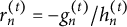
Convergence: A simpler rule, such as $\ell ^{(t)} - \ell ^{(t-1)} < \varepsilon $
(absolute or relative change in consecutive log-likelihoods), is often used but can be unreliable in the proposed algorithm. It may halt prematurely after a transient small change—caused, for instance, by noise in the XGBoost fit or by approximation error in the Laplace step—or fail to detect mild oscillations that indicate a lack of convergence. Accordingly, convergence is assessed via stability of the (approximate) log-likelihood over a rolling window of recent iterations. Let
$\ell ^{(t)} - \ell ^{(t-1)} < \varepsilon $
(absolute or relative change in consecutive log-likelihoods), is often used but can be unreliable in the proposed algorithm. It may halt prematurely after a transient small change—caused, for instance, by noise in the XGBoost fit or by approximation error in the Laplace step—or fail to detect mild oscillations that indicate a lack of convergence. Accordingly, convergence is assessed via stability of the (approximate) log-likelihood over a rolling window of recent iterations. Let $L \ge 2$
denote a user-specified window length. The stability check is first applied only once L log-likelihood values are available, that is, for
$L \ge 2$
denote a user-specified window length. The stability check is first applied only once L log-likelihood values are available, that is, for $t \ge L-1$
; the condition
$t \ge L-1$
; the condition $t \ge 4$
in Algorithm 1 corresponds to the illustrative choice
$t \ge 4$
in Algorithm 1 corresponds to the illustrative choice $L=5$
. The algorithm terminates the iteration if the following condition holds:
$L=5$
. The algorithm terminates the iteration if the following condition holds: $t \ge L-1$
and
$t \ge L-1$
and
 $$\begin{align*}\operatorname{SD}\!\bigl(\ell^{(t-L+1)},\ldots,\ell^{(t)}\bigr) < \varepsilon, \end{align*}$$
where $\varepsilon>0$
is a user-specified tolerance and
$\varepsilon>0$
is a user-specified tolerance and $\operatorname {SD}\!\bigl (\ell ^{(t-L+1)},\ldots ,\ell ^{(t)}\bigr )$
denotes the sample standard deviation of the most recent L log-likelihood values, that is,
$\operatorname {SD}\!\bigl (\ell ^{(t-L+1)},\ldots ,\ell ^{(t)}\bigr )$
denotes the sample standard deviation of the most recent L log-likelihood values, that is,
 $$\begin{align*}\operatorname{SD}\!\bigl(\ell^{(t-L+1)},\ldots,\ell^{(t)}\bigr) = \sqrt{\frac{1}{L-1}\sum_{s=t-L+1}^{t}\Big(\ell^{(s)}-\bar{\ell}^{(t)}\Big)^2}, \qquad \bar{\ell}^{(t)}=\frac{1}{L}\sum_{s=t-L+1}^{t}\ell^{(s)}. \end{align*}$$
Both L (window length) and the earliest iteration at which the stability check is activated are user-configurable, allowing the convergence criterion to be tuned for robustness to transient fluctuations. Otherwise set $t \leftarrow t + 1$
and repeat.
$t \leftarrow t + 1$
and repeat.
Unlike a strict EM algorithm, the E-step in the iterative GLMM–XGBoost algorithm does not integrate over the full conditional distribution of the random effects. Instead, it updates the fixed-effects function $f(\mathbf {x})$
via a weighted regression of working residuals, conditional on current empirical Bayes predictions of the random effects. Consequently, classical EM guarantees (e.g., monotonicity of the likelihood and convergence to a stationary point) do not formally apply. Nevertheless, in practice, we typically observe near-monotone sequences of the Laplace-approximated marginal log-likelihood and stable convergence of both the variance components and the fixed intercept.
$f(\mathbf {x})$
via a weighted regression of working residuals, conditional on current empirical Bayes predictions of the random effects. Consequently, classical EM guarantees (e.g., monotonicity of the likelihood and convergence to a stationary point) do not formally apply. Nevertheless, in practice, we typically observe near-monotone sequences of the Laplace-approximated marginal log-likelihood and stable convergence of both the variance components and the fixed intercept.
Tuning parameters: Several user-controlled constants govern the behavior and stability of the algorithm:
-
• Hyperparameter selection for XGBoost: Run cluster K-fold cross-validation (CV) stratified by clusters: for each candidate set of tuning parameters, compute the average out-of-cluster validation error across folds and select the configuration with the best cross-validated performance.
-
• Tolerance
$\ \varepsilon $
: Threshold used in the stopping rule based on the standard deviation of recent log-likelihoods (e.g., the last three iterations); smaller values enforce tighter convergence at the expense of run time. -
• Learning rate
$\ \alpha _{L}$
: Controls the influence of the newly fitted XGBoost on the offset. Smaller
$\alpha _{L}$
produces more conservative updates and can improve stability at the cost of extra iterations.


The use of cluster K-fold CV stratified by clusters for XGBoost is motivated by the multilevel nature of the binary item response data. Standard row-wise splits can leak information across levels, because individuals from the same cluster may appear in both training and validation sets. This induces overly optimistic validation performance, as the model can exploit cluster-specific patterns that do not generalize to new clusters. By contrast, cluster-level folds ensure that all individuals within a cluster are assigned to either the training or validation set, so that validation error reflects true out-of-cluster generalization. The stratification step further preserves the outcome prevalence across folds, stabilizing error estimates. To avoid nested CV at every E-step and to promote stable EM-like updates, the cluster-stratified K-fold hyperparameter tuning is performed once prior to the loop and hold the resulting configuration fixed across iterations; only the working residuals and precision weights are updated at each iteration.
Effective implementation hinges on the strategic choice of the user-controlled constants governing the algorithm’s behavior. Hyperparameters for XGBoost can be selected by strategically constraining the grid based on the data complexities (e.g., $N \approx 4.7 \times 10^{4}$
records across 32 schools) and the properties of the residual-learning task. For instance, the maximum depth (d) and minimum child weight can be constrained to ensure a sufficient number of effective observations per terminal node (e.g.,
$N \approx 4.7 \times 10^{4}$
records across 32 schools) and the properties of the residual-learning task. For instance, the maximum depth (d) and minimum child weight can be constrained to ensure a sufficient number of effective observations per terminal node (e.g., $\approx N / 2^{d}$
) to mitigate high variance under clustering. In addition, the learning rate (
$\approx N / 2^{d}$
) to mitigate high variance under clustering. In addition, the learning rate ( $\alpha _{L}$
) determines the influence of the newly fitted XGBoost on the offset (Equation (14)) and serves as the primary control for convergence stability. Given the EM-like nature of the updates, users may start with smaller
$\alpha _{L}$
) determines the influence of the newly fitted XGBoost on the offset (Equation (14)) and serves as the primary control for convergence stability. Given the EM-like nature of the updates, users may start with smaller $\alpha _{L}$
values (e.g.,
$\alpha _{L}$
values (e.g., $0.05$
–
$0.05$
– $0.2$
) to ensure conservative, stable steps, accepting a trade-off that increases the total number of iterations required for convergence. However, if preliminary testing shows that the GLMM estimates remain similar across multiple
$0.2$
) to ensure conservative, stable steps, accepting a trade-off that increases the total number of iterations required for convergence. However, if preliminary testing shows that the GLMM estimates remain similar across multiple $\alpha _{L}$
values, a moderate learning rate, such as
$\alpha _{L}$
values, a moderate learning rate, such as $0.5$
, can be chosen to aggressively reduce the total number of iterations. For the robust convergence check, the rolling-window SD criterion requires tuning both the tolerance
$0.5$
, can be chosen to aggressively reduce the total number of iterations. For the robust convergence check, the rolling-window SD criterion requires tuning both the tolerance $\varepsilon $
and the window length L. A smaller tolerance
$\varepsilon $
and the window length L. A smaller tolerance $\varepsilon $
enforces a tighter definition of convergence stability, while a larger window length L (e.g.,
$\varepsilon $
enforces a tighter definition of convergence stability, while a larger window length L (e.g., $L \ge 5$
) is essential for improving the robustness of the stability check against transient fluctuations in the log-likelihood. Users must select these parameters to balance the need for tight convergence (small
$L \ge 5$
) is essential for improving the robustness of the stability check against transient fluctuations in the log-likelihood. Users must select these parameters to balance the need for tight convergence (small $\varepsilon $
) against the practical need for reasonable runtime (higher
$\varepsilon $
) against the practical need for reasonable runtime (higher $\alpha _L$
, smaller L).
$\alpha _L$
, smaller L).

2.3 Group-aware conditional permutation importance
Permutation importance quantifies how much predictive performance deteriorates when the values of a given predictor are randomly permuted without replacement (thereby breaking its association with the target) while all other predictors remain intact; a larger deterioration implies greater importance. The substantive question answered by this measure is conditional rather than marginal: holding the fitted random-effects structure fixed, how much does a given fixed predictor $x_q$
uniquely improve prediction of the working-residual target
$x_q$
uniquely improve prediction of the working-residual target $r_n$
beyond what is already explained by the remaining predictors? In the iterative GLMM–XGBoost framework, this interpretation is “net of” modeled group heterogeneity because the GLMM step accounts for cross-classified random intercepts and the residual learner is constrained (via the weighted C-projection) to avoid absorbing variation in the group-dummy space. This contrasts with standard marginal importance computed on the original outcome, which can conflate fixed-effect signal with dependence induced by unmodeled or insufficiently controlled random effects.
$r_n$
beyond what is already explained by the remaining predictors? In the iterative GLMM–XGBoost framework, this interpretation is “net of” modeled group heterogeneity because the GLMM step accounts for cross-classified random intercepts and the residual learner is constrained (via the weighted C-projection) to avoid absorbing variation in the group-dummy space. This contrasts with standard marginal importance computed on the original outcome, which can conflate fixed-effect signal with dependence induced by unmodeled or insufficiently controlled random effects.
In this study, permutation is implemented using a group-aware scheme that respects the multilevel design. Predictors are shuffled at their designated level (person, cluster, and item), and permuted values are copied back to all rows within the same group to preserve within-group constancy. For example, for cluster-centered person-level predictors, permutations are restricted within persons to preserve centering and marginal distributions. This procedure disrupts only the predictor–target association while preserving the multilevel structure, yielding less biased importance estimates than naïve row-wise shuffling.
Specifically, in the iterative GLMM–XGBoost algorithm, the final residual learner $\tilde {f}(\mathbf {x}_n)$
is trained on IRLS working-residual targets
$\tilde {f}(\mathbf {x}_n)$
is trained on IRLS working-residual targets $r_n$
with observation weights
$r_n$
with observation weights $\omega _n$
. Importance is computed using the same group-aware permutation scheme and a weight-aware error metric. Baseline predictions and the weighted error metric are
$\omega _n$
. Importance is computed using the same group-aware permutation scheme and a weight-aware error metric. Baseline predictions and the weighted error metric are
 $$ \begin{align} \hat{r}_n^{(0)} = \tilde{f}(\mathbf{x}_n), \qquad \mathrm{MSE}_w(\tilde{f}) = \frac{\sum_{n=1}^N \omega_n (r_n - \hat{r}_n^{(0)})^2}{\sum_{n=1}^N \omega_n}, \quad \bar{r}_w = \frac{\sum_{n=1}^N \omega_n r_n}{\sum_{n=1}^N \omega_n}, \end{align} $$
with $\mathrm {RMSE}_w = \sqrt {\mathrm {MSE}_w}$
used in this study. The use of the IRLS precision weight
$\mathrm {RMSE}_w = \sqrt {\mathrm {MSE}_w}$
used in this study. The use of the IRLS precision weight $\omega _n$
in the error metric is mathematically justified because
$\omega _n$
in the error metric is mathematically justified because $r_n$
arises from the local WLS sub-problem underlying the IRLS/Newton (Fisher-scoring) update (Section 2.2.1). For Bernoulli data with a logit link,
$r_n$
arises from the local WLS sub-problem underlying the IRLS/Newton (Fisher-scoring) update (Section 2.2.1). For Bernoulli data with a logit link, $\omega _n = p_n(1-p_n)$
equals the curvature (Fisher information) of the local quadratic approximation to the negative log-likelihood. Consequently,
$\omega _n = p_n(1-p_n)$
equals the curvature (Fisher information) of the local quadratic approximation to the negative log-likelihood. Consequently, $\mathrm {MSE}_w$
weights squared prediction errors according to their local precision in the IRLS sub-problem, aligning the permutation-based importance calculation with the objective that defines the fixed-effects update.
$\mathrm {MSE}_w$
weights squared prediction errors according to their local precision in the IRLS sub-problem, aligning the permutation-based importance calculation with the objective that defines the fixed-effects update.
For a given predictor $x_q$
, let
$x_q$
, let $\pi _q$
denote a random permutation of
$\pi _q$
denote a random permutation of $x_q$
within groups, preserving the multilevel structure while breaking its association with the target. The corresponding predictions and permuted metric are
$x_q$
within groups, preserving the multilevel structure while breaking its association with the target. The corresponding predictions and permuted metric are
 $$ \begin{align} \hat{r}_n^{(\pi_q)} = \tilde{f}(\mathbf{x}_n^{\pi_q}), \quad M_q = M \big( \{(r_n, \hat{r}_n^{(\pi_q)}, \omega_n) : n=1,\dots,N\} \big), \quad M_0 = M \big( \{(r_n, \hat{r}_n^{(0)}, \omega_n) : n=1,\dots,N\} \big). \end{align} $$
The full-sample group-aware permutation importance is the expected increase in error, averaged over R independent permutations:
 $$ \begin{align} \widehat{\Delta}_q = \frac{1}{R} \sum_{r=1}^R \big( M_{q,r} - M_0 \big). \end{align} $$
For interpretability, a normalized relative importance rescales the nonnegative effects to sum to one:
 $$ \begin{align} \mathrm{RelImp}_q = \frac{\max \big( \widehat{\Delta}_q, 0 \big)}{\sum_j \max \big( \widehat{\Delta}_j, 0 \big)}. \end{align} $$
This measure reflects the proportion of predictive accuracy attributable to each predictor under group-aware, full-sample permutation, accounting for the IRLS weighting scheme $\omega _n$
.
$\omega _n$
.
Uncertainty and significance were further assessed from the empirical distribution of the permutation effects. The variability of predictor $x_q$
was summarized by the sample standard deviation of the R replicate effects:
$x_q$
was summarized by the sample standard deviation of the R replicate effects:
 $$ \begin{align} \Delta_{q,sd} = \sqrt{\frac{1}{R-1}\sum_{r=1}^R \Big[ (M_{q,r} - M_0) - \widehat{\Delta}_q \Big]^2 }. \end{align} $$
In addition, nonparametric percentile confidence interval for predictor $x_q$
can be obtained from the empirical quantiles of
$x_q$
can be obtained from the empirical quantiles of $\{M_{q,r} - M_0 : r=1,\dots ,R\}$
:
$\{M_{q,r} - M_0 : r=1,\dots ,R\}$
:
 $$ \begin{align} \mathrm{CI}_{q,(1-\alpha_{1})} = \Big[\, Q_{\alpha_{1}/2}(\,M_{q,r} - M_0\,), \; Q_{1-\alpha_{1}/2}(\,M_{q,r} - M_0\,) \,\Big], \end{align} $$
where $\alpha _{1}$
denotes the significance level and
$\alpha _{1}$
denotes the significance level and $Q_p$
denotes the pth sample quantile.
$Q_p$
denotes the pth sample quantile.
In addition to the full-sample, group-aware permutation importance, this study also provides a K-fold out-of-fold (OOF) permutation importance with cluster CV for generalization. In this framework, permutation importance is estimated using the final fitted GLMM–XGBoost model while holding out entire clusters (e.g., schools within which students are nested). For each validation fold, predictions are obtained on the held-out clusters, baseline errors are computed, and then group-aware permutations of predictor $x_q$
are applied within the fold to break predictor–outcome associations without altering the multilevel structure. The increase in prediction error due to permutation is averaged across permutations within each fold and then aggregated across all folds to yield the OOF importance estimate.
$x_q$
are applied within the fold to break predictor–outcome associations without altering the multilevel structure. The increase in prediction error due to permutation is averaged across permutations within each fold and then aggregated across all folds to yield the OOF importance estimate.
By explicitly modeling random effects and incorporating group-aware permutations, the group-aware conditional permutation measure from the GLMM–XGBoost framework yields predictor rankings that more accurately reflect fixed-effect contributions while accounting for clustering at the person, cluster, and item levels. When data are clustered, marginal and conditional importance address different scientific questions: marginal scores reflect overall predictive power across both within- and between-group variation, whereas conditional scores isolate the unique contribution of fixed effects net of random heterogeneity. Importance scores from XGBoost, which assumes independence and relies on row-wise shuffling, can therefore conflate fixed and random sources of variation. In particular, with non-negligible intra-class correlation (ICC), ignoring grouping may cause importance weights to mix within- and between-cluster signals, inflating predictors correlated with the random effects and deflating others.
3 Empirical study
In this section, the iterative GLMM–XGBoost algorithm is applied to the empirical dataset with the empirical aim of identifying important predictors.
3.1 Data
The publicly available version of the Add Health Wave I data (Harris & Udry, Reference Harris and Udry2022) was chosen to illustrate the iterative GLMM–XGBoost algorithm. This dataset includes 6,504 participants nested within 132 schools. For illustrative purposes, schools with a large number of students (i.e., greater than 61, corresponding to the third quantile of the number of students across the 132 schools) were selected to allow stable estimation in the multilevel data, resulting in 2,471 students nested within 32 schools. The number of students per school (cluster size) ranged from 62 to 122 (median = 79; IQR = 20.5). This restriction to relatively large schools facilitates stable estimation but may limit generalizability, as the resulting importance rankings may primarily reflect patterns in larger schools and may not fully extend to smaller schools with different within-cluster variability, measurement precision, and contextual characteristics.
The binary outcomes were derived from the 19-item modified version of the Center for Epidemiologic Studies Depression Scale (CES-D; Perreira et al., Reference Perreira, Deeb-Sossa, Harris and Bollen2005; Radloff, Reference Radloff1977), which has demonstrated good internal consistency in prior Add Health work (Wight et al., Reference Wight, Aneshensel, Botticello and Sepúlveda2005). Each item (H1FS1–H1FS19) was administered with four response categories: 0 = “never or rarely” ( $<$
1 day in the past week), 1 = “sometimes” (1–2 days), 2 = “a lot of the time” (3–4 days), and 3 = “most or all of the time” (5–7 days). Responses of “refused” (6), “don’t know” (8), and “not applicable” (9) were treated as missing. Consistent with the DSM-5 criterion that depressive symptoms must occur nearly every day to be clinically meaningful, items were dichotomised such that responses of 0 or 1 were coded as symptom absent (0), and responses of 2 or 3 were coded as symptom present (1). The four positive-affect items (H1FS4, H1FS8, H1FS11, and H1FS15) were reverse-coded prior to dichotomisation so that higher values consistently indicate greater depressive symptomatology. The resulting binary items capture the presence or absence of depressive symptoms at clinically relevant frequency while minimizing the influence of transient or subclinical mood fluctuations.
$<$
1 day in the past week), 1 = “sometimes” (1–2 days), 2 = “a lot of the time” (3–4 days), and 3 = “most or all of the time” (5–7 days). Responses of “refused” (6), “don’t know” (8), and “not applicable” (9) were treated as missing. Consistent with the DSM-5 criterion that depressive symptoms must occur nearly every day to be clinically meaningful, items were dichotomised such that responses of 0 or 1 were coded as symptom absent (0), and responses of 2 or 3 were coded as symptom present (1). The four positive-affect items (H1FS4, H1FS8, H1FS11, and H1FS15) were reverse-coded prior to dichotomisation so that higher values consistently indicate greater depressive symptomatology. The resulting binary items capture the presence or absence of depressive symptoms at clinically relevant frequency while minimizing the influence of transient or subclinical mood fluctuations.
To create item-level predictors, the 19 CES-D items (H1FS1–H1FS19) were organized into content-homogeneous domains supported by prior psychometric work in adolescents and adults (Radloff, Reference Radloff1977; Wight et al., Reference Wight, Aneshensel, Botticello and Sepúlveda2005). The domains correspond to four canonical subscales—Depressed Affect (I_depressedaffect; H1FS1, H1FS3, H1FS6, H1FS9, H1FS10, H1FS13, H1FS16), Somatic and Retarded Activity (I_somatic; H1FS2, H1FS5, H1FS7, H1FS12, H1FS18), Positive Affect (I_positiveaffect; H1FS4, H1FS8, H1FS11, H1FS15, reverse-coded), and Interpersonal Problems (I_interpersonal; H1FS14, H1FS17)—plus a separate Suicidal Ideation item (H1FS19), which is routinely analyzed independently because of its distinct clinical meaning. For analysis, each domain except a Suicidal Ideation item was dummy-coded as an item-level predictor (e.g., 1 = item belongs to the domain, 0 = otherwise). These predictors do not vary across individuals but instead describe structural attributes of the items, allowing the multilevel model to account for systematic differences in response tendencies across item content domains.
Based on prior studies using Add Health data to examine depressive symptoms (e.g., Sowislo & Orth, Reference Sowislo and Orth2013), six individual-level predictors were selected from the public-use Add Health Wave I dataset: parents’ education (Peducation), self-esteem (selfesteem), social support (socialsupport), overall GPA (overall_GPA), delinquency (delinquent), and family income (familyincome). For the categorical variable of parents’ education, three dummy variables (high school graduate, some college, and college graduate; Peducation_High.school.graduate; Peducation_Some. college; Peducation_College.graduate) were created, with less than high school as the reference category. All other continuous predictors were standardized. These predictors were decomposed into within-level predictors (representing “pure” individual-level effects; W_*) and between-level predictors (i.e., cluster means of the individual-level predictors; B_*).
To summarize the data structure, the dataset comprises 46,949 binary responses from 2,471 students cross-classified with 19 items; students are nested within 32 schools. The dataset includes 20 predictors: eight individual-level (within-cluster), eight cluster-level (between-cluster), and four item-level predictors.
3.2 Analysis
Data were arranged in long format, with each row representing a unique student–item pair within a school. Among the 20 predictors, there were no zero-variance predictors, no highly correlated predictors, and no linear dependencies. The median correlation among predictors was 0.000, and the interquartile range was 0.038. Sixty-seven observations had missing outcomes (0.143% of the original 46,949) and were removed.
Predictor missingness was addressed via multiple imputation. Specifically, missing values in both continuous and categorical predictors—arising from responses, such as “does not apply,” “refused,” or “don’t know”—were recoded as NA and subsequently imputed using the random forest method implemented in the mice package (van Buuren & Groothuis-Oudshoorn, Reference van Buuren and Groothuis-Oudshoorn2011). All predictors were imputed jointly using the remaining predictors as inputs, and the completed dataset was used for subsequent analyses. Consequently, no cases were excluded due to missing predictor values.
The ICCs based on the GLMM without any predictors were 0.321 ( $=\widehat {\sigma }_{\theta }^{2}/(\widehat {\sigma }_{\theta }^{2}+\widehat {\sigma }_{\alpha }^{2}+\widehat {\sigma }_{\delta }^{2}+\pi ^2/3)$
), 0.141
$=\widehat {\sigma }_{\theta }^{2}/(\widehat {\sigma }_{\theta }^{2}+\widehat {\sigma }_{\alpha }^{2}+\widehat {\sigma }_{\delta }^{2}+\pi ^2/3)$
), 0.141 $=\widehat {\sigma }_{\delta }^{2}/(\widehat {\sigma }_{\theta }^{2}+\widehat {\sigma }_{\alpha }^{2}+\widehat {\sigma }_{\delta }^{2}+\pi ^2/3)$
, and 0.015
$=\widehat {\sigma }_{\delta }^{2}/(\widehat {\sigma }_{\theta }^{2}+\widehat {\sigma }_{\alpha }^{2}+\widehat {\sigma }_{\delta }^{2}+\pi ^2/3)$
, and 0.015 $=\widehat {\sigma }_{\alpha }^{2}/(\widehat {\sigma }_{\theta }^{2}+\widehat {\sigma }_{\alpha }^{2}+\widehat {\sigma }_{\delta }^{2}+\pi ^2/3)$
for students, items, and schools, respectively. These ICCs indicate non-negligible correlations in latent responses attributable to the cross-classified structure of students and items and to students nested within schools. Using the school-level ICC and median cluster size=79, the design effect is
$=\widehat {\sigma }_{\alpha }^{2}/(\widehat {\sigma }_{\theta }^{2}+\widehat {\sigma }_{\alpha }^{2}+\widehat {\sigma }_{\delta }^{2}+\pi ^2/3)$
for students, items, and schools, respectively. These ICCs indicate non-negligible correlations in latent responses attributable to the cross-classified structure of students and items and to students nested within schools. Using the school-level ICC and median cluster size=79, the design effect is $1 + (\mathrm {cluster size}-1) \times \mathrm {ICC} \approx 2.17$
, implying an effective information fraction of
$1 + (\mathrm {cluster size}-1) \times \mathrm {ICC} \approx 2.17$
, implying an effective information fraction of $1/2.17 \approx 0.46$
relative to simple random sampling and justifying a multilevel specification with a school random intercept.
$1/2.17 \approx 0.46$
relative to simple random sampling and justifying a multilevel specification with a school random intercept.
For comparison, GLMM–XGBoost, XGBoost (binary classification), and a GLMM with linear main effects were fitted to the same empirical dataset. Comparing XGBoost with GLMM–XGBoost underscores the added modeling of random effects for students, items, and schools. In addition, comparing the GLMM with GLMM–XGBoost highlights the additional flexibility to capture potential interactions and nonlinearities. The GLMM included only linear main effects because it serves as a baseline model for comparison. This choice does not imply that GLMMs cannot accommodate interactions or nonlinearities; rather, it establishes a standard reference point for assessing whether a data-driven approach, such as GLMM–XGBoost, improves explanatory performance relative to a traditionally specified GLMM. XGBoost was fitted using the xgboost function from the xgboost package, and the GLMM was fitted using the glmer function from the lme4 package. The estimation method outlined in Section 2 was used to fit the GLMM–XGBoost model.
In the residual-learning stage of GLMM–XGBoost and XGBoost, hyperparameters were selected using a grid search to balance capacity and stability under the empirical design (2,471 students within 32 schools; 19 items per student; school cluster sizes 62–122, median =79, IQR =20.5). The learning rate (eta) was tuned as $\in {0.02, 0.03, 0.05}$
and the maximum tree depth (max depth) as
$\in {0.02, 0.03, 0.05}$
and the maximum tree depth (max depth) as $d \in {3, 4, 5}$
, constraining interaction order; for
$d \in {3, 4, 5}$
, constraining interaction order; for $N \approx 4.7 \times 10^{4}$
person–item records, the expected observations per terminal node are approximately
$N \approx 4.7 \times 10^{4}$
person–item records, the expected observations per terminal node are approximately $N / 2^{d}$
(i.e.,
$N / 2^{d}$
(i.e., $\approx 5.9 \times 10^{3}$
,
$\approx 5.9 \times 10^{3}$
, $2.9 \times 10^{3}$
, and
$2.9 \times 10^{3}$
, and $1.5 \times 10^{3}$
for
$1.5 \times 10^{3}$
for $d=3,4,5$
). Because IRLS weights were normalized to mean
$d=3,4,5$
). Because IRLS weights were normalized to mean $\approx 1$
, the minimum child weight (min child weight) was treated as a lower bound on effective sample size per leaf; the grid
$\approx 1$
, the minimum child weight (min child weight) was treated as a lower bound on effective sample size per leaf; the grid $\texttt {min child weight} \in {25, 50, 75}$
enforced at least 25–75 effective cases per leaf to mitigate variance under clustering.
$\texttt {min child weight} \in {25, 50, 75}$
enforced at least 25–75 effective cases per leaf to mitigate variance under clustering. $\ell _{2}$
regularization (lambda) explored
$\ell _{2}$
regularization (lambda) explored $\lambda \in {1, 3, 10}$
to shrink leaf values
$\lambda \in {1, 3, 10}$
to shrink leaf values $\omega ^{*} = -G / (H + \lambda )$
and stabilize small partitions. For the
$\omega ^{*} = -G / (H + \lambda )$
and stabilize small partitions. For the $\ell _1$
penalty, alpha was set to
$\ell _1$
penalty, alpha was set to ${0, 0.1, 0.5, 1, 3}$
. Under XGBoost’s second-order objective, the optimal leaf value is
${0, 0.1, 0.5, 1, 3}$
. Under XGBoost’s second-order objective, the optimal leaf value is $\omega ^{*} \;=\; -\,(H + \lambda )^{-1} \, \operatorname {sgn}(G)\, \max \!\bigl (|G| - \alpha ,\,0\bigr )$
(Chen & Guestrin, Reference Chen and Guestrin2016), so alpha=
$\omega ^{*} \;=\; -\,(H + \lambda )^{-1} \, \operatorname {sgn}(G)\, \max \!\bigl (|G| - \alpha ,\,0\bigr )$
(Chen & Guestrin, Reference Chen and Guestrin2016), so alpha= $\alpha $
implements soft-thresholding on the summed gradient G while lambda=
$\alpha $
implements soft-thresholding on the summed gradient G while lambda= $\lambda $
inflates curvature H (ridge shrinkage). With IRLS weights normalized to
$\lambda $
inflates curvature H (ridge shrinkage). With IRLS weights normalized to $1$
, the leaf curvature H is approximately the effective leaf size, which is constrained to be at least 25–100 by min child weight. On this scale,
$1$
, the leaf curvature H is approximately the effective leaf size, which is constrained to be at least 25–100 by min child weight. On this scale, $\alpha \in [0.5, 3]$
induces mild-to-moderate sparsity: it zeroes leaves whose signal is near noise while preserving substantive effects, complementing the smoother
$\alpha \in [0.5, 3]$
induces mild-to-moderate sparsity: it zeroes leaves whose signal is near noise while preserving substantive effects, complementing the smoother $\ell _2$
shrinkage from
$\ell _2$
shrinkage from $\lambda \in {1, 3, 10}$
. Including
$\lambda \in {1, 3, 10}$
. Including $\alpha = 0$
ensures a baseline without
$\alpha = 0$
ensures a baseline without $\ell _1$
regularization;
$\ell _1$
regularization; $\alpha = 0.5$
–1 provides light sparsity that can reduce variance when residual signal is diffuse across many predictors; and
$\alpha = 0.5$
–1 provides light sparsity that can reduce variance when residual signal is diffuse across many predictors; and $\alpha = 3$
offers a stronger option for sensitivity analyses or when deeper trees produce many small-contribution leaves. Larger
$\alpha = 3$
offers a stronger option for sensitivity analyses or when deeper trees produce many small-contribution leaves. Larger $\alpha $
values were avoided to prevent over-sparsification given moderate H. The search permitted up to num boost round=1,200 with early stopping and used RMSE as the tuning criterion. Hyperparameter selection used group K-fold CV by school (
$\alpha $
values were avoided to prevent over-sparsification given moderate H. The search permitted up to num boost round=1,200 with early stopping and used RMSE as the tuning criterion. Hyperparameter selection used group K-fold CV by school ( $K=5$
), with subsampling ratios fixed at colsample bytree=0.8 and subsample=1.0 to avoid cross-cluster leakage. For GLMM–XGBoost, the selected configuration was eta = 0.02, max depth = 3, min child weight = 25, lambda = 10, and alpha = 0.5, with early stopping at 256 boosting rounds. For XGBoost, the selected configuration was eta = 0.05, max depth = 4, min child weight = 75, lambda = 3, and alpha = 0, with early stopping at 114 boosting rounds.
$K=5$
), with subsampling ratios fixed at colsample bytree=0.8 and subsample=1.0 to avoid cross-cluster leakage. For GLMM–XGBoost, the selected configuration was eta = 0.02, max depth = 3, min child weight = 25, lambda = 10, and alpha = 0.5, with early stopping at 256 boosting rounds. For XGBoost, the selected configuration was eta = 0.05, max depth = 4, min child weight = 75, lambda = 3, and alpha = 0, with early stopping at 114 boosting rounds.
Figure 1 plots the observed log-likelihood across 22 iterations in the iterative GLMM–XGBoost with $\alpha _{L}=0.5$
. The fit improves rapidly over the first five iterations and then enters a stable plateau with small, bounded oscillations. The standard deviation of the log-likelihood across the last three iterations is about 0.24, and the GLMM estimates differ only in the fourth decimal place across these iterations, providing evidence of convergence by iteration 22.
$\alpha _{L}=0.5$
. The fit improves rapidly over the first five iterations and then enters a stable plateau with small, bounded oscillations. The standard deviation of the log-likelihood across the last three iterations is about 0.24, and the GLMM estimates differ only in the fourth decimal place across these iterations, providing evidence of convergence by iteration 22.
Empirical study: Log-likelihood values over iterations in the iterative GLMM–XGBoost.

To illustrate differences among GLMM–XGBoost, XGBoost, and GLMM, full-sample performance metrics (AUC and Brier score) are reported, recognizing that these quantities reflect model behavior on different evaluative scales (conditional vs. marginal vs. non-hierarchical) rather than out-of-sample generalization. The group-aware conditional permutation importance described in Section 2.3 was computed from the final GLMM–XGBoost fit (iteration 22). For XGBoost, the standard (global shuffle and unconditional) permutation importance was used. One thousand permutations were employed for both the group-aware conditional permutation and the standard permutation importance measures.
Computation time was recorded using elapsed time from system.time() in R and (for GLMM–XGBoost) the stage-wise timing log produced by the implementation. The baseline GLMM required 12.85 minutes. For standalone XGBoost, hyperparameter tuning (grid search with CV) plus the final refit required 154.84 minutes, and the global permutation importance analysis with 1,000 replications required 21.80 minutes, yielding a combined total of 176.64 minutes (2.94 hours) for these two components. For GLMM–XGBoost, the XGBoost tuning step required 151.69 minutes, the EM-style iterative estimation required 368.61 minutes, and the full-sample permutation importance procedure with 1,000 replications required an additional 21.11 minutes, yielding a combined total of 541.41 minutes (9.02 hours) for these components. All computations were conducted on a laptop equipped with an Intel(R) Core(TM) i7-1065G7 CPU @ 1.30 GHz.
3.3 Results
Using conditional predictions (i.e., predictions incorporating estimated random effects) from the final GLMM–XGBoost fit (iteration 22), classification performance for the binary endorsement outcome was high (AUC = 0.900, 95% CI = [0.896, 0.904]) with a low Brier score (0.070). On the marginal scale, integrating over random effects, performance was lower (AUC = 0.722, 95% CI = [0.715, 0.730]; Brier = 0.106). The gap between conditional and marginal metrics is consistent with substantial heterogeneity across students, schools, and items: conditioning on random effects yields more individualized predictions, whereas marginal predictions reflect average performance across groups. For the final XGBoost model fit on all observations (full-sample evaluation), performance was intermediate (AUC = 0.801, 95% CI = [0.795, 0.807]; Brier = 0.086). Because XGBoost does not explicitly model random effects, its predictions are evaluated on a non-hierarchical scale; its intermediate performance may reflect predictive structure captured through observed covariates that are correlated with clustering. The GLMM with linear main effects showed lower discrimination and higher Brier scores than GLMM–XGBoost on both the conditional and marginal scales (conditional AUC = 0.780, 95% CI = [0.770, 0.799], Brier = 0.090; marginal AUC = 0.699, 95% CI = [0.670, 0.701], Brier = 0.121). These results suggest that, in this dataset, the added flexibility of GLMM–XGBoost to represent nonlinearities and interactions was associated with improved full-sample predictive performance relative to a linear main-effects GLMM.
The random effects from GLMM–XGBoost revealed heterogeneity across multiple levels: person-level variance was the largest (Var = 1.759, SD = 1.326), followed by item-level variance (Var = 0.845, SD = 0.919), and smaller but nontrivial school-level variance (Var = 0.084, SD = 0.289). These variance components represented random residuals after accounting for the predictors, quantifying the remaining unexplained variability at each level of the hierarchy. Specifically, even after predictor adjustment, individual participants differed markedly in their propensity for endorsement, items varied substantially in easiness (i.e., the negative of difficulty), and schools showed modest differences in overall endorsement levels. When random effects were modeled in GLMM–XGBoost, predictor importance rankings reflected this partitioning of variance.
Table 1 presents a comparison of permutation-importance measures: group-aware conditional permutation importance from GLMM–XGBoost versus standard (global shuffle and unconditional) permutation importance from XGBoost. As shown in Table 1, although the overall rank correlation between GLMM–XGBoost and standard XGBoost was moderately high (Spearman’s rho = 0.801), nontrivial rank discrepancies—especially among item- and cluster-level predictors—were evident.Footnote
3
Specifically, GLMM–XGBoost identified W_selfesteem as the most important predictor, whereas standard XGBoost ranked I_positiveaffect highest. The largest contrast was observed for I_interpersonal, which ranked 9 in GLMM–XGBoost but 16 in XGBoost, reflecting a substantial difference between the two methods. Among person-level predictors, rank differences were comparatively modest: across the eight W_* variables, the XGBoost-minus-GLMM–XGBoost rank differences ranged from $-2$
to
$-2$
to $+2$
. By contrast, larger differences in ranks were found for item-level and cluster-level predictors. Item-level predictors such as I_depressedaffect, I_somatic, I_positiveaffect, and I_interpersonal ranked 7, 4, 3, and 9, respectively, in GLMM–XGBoost, whereas the same predictors were ranked 11, 5, 1, and 16, respectively, in XGBoost. Cluster-level predictors (e.g., B_familyincome, B_socialsupport, and B_selfesteem) also showed variation, with higher relative importance in XGBoost compared to GLMM–XGBoost. For instance, B_familyincome ranked 13 in GLMM–XGBoost versus 8 in XGBoost, B_socialsupport ranked 15 versus 9, and B_selfesteem ranked 17 versus 3.
$+2$
. By contrast, larger differences in ranks were found for item-level and cluster-level predictors. Item-level predictors such as I_depressedaffect, I_somatic, I_positiveaffect, and I_interpersonal ranked 7, 4, 3, and 9, respectively, in GLMM–XGBoost, whereas the same predictors were ranked 11, 5, 1, and 16, respectively, in XGBoost. Cluster-level predictors (e.g., B_familyincome, B_socialsupport, and B_selfesteem) also showed variation, with higher relative importance in XGBoost compared to GLMM–XGBoost. For instance, B_familyincome ranked 13 in GLMM–XGBoost versus 8 in XGBoost, B_socialsupport ranked 15 versus 9, and B_selfesteem ranked 17 versus 3.
Empirical study: Permutation importance comparisons between GLMM–XGBoost and XGBoost

Note: Ranks are computed within method by sorting RelImp in descending order. “Rank Diff” = Rank $_{\text {XGB}} \ -$
Rank
$_{\text {XGB}} \ -$
Rank $_{\text {GLMM--XGB}}$
; negative values indicate the feature ranked higher under XGBoost than under GLMM–XGBoost.
$_{\text {GLMM--XGB}}$
; negative values indicate the feature ranked higher under XGBoost than under GLMM–XGBoost.
The variable-importance patterns identified by GLMM–XGBoost align with established findings in the adolescent depression literature while clarifying how multilevel dependence shapes the apparent influence of predictors. At the individual level, self-esteem and perceived social support emerged as the most influential predictors, consistent with extensive evidence that negative self-evaluation and deficits in social support are core correlates of adolescent depressive symptoms (Harter, Reference Harter1999; Orth et al., Reference Orth, Robins and Roberts2008). Their high rankings under GLMM–XGBoost indicate that these predictors remain important even after accounting for unobserved heterogeneity across students, schools, and items, suggesting that their associations with depressive symptom endorsement are not solely driven by clustering or measurement-related artifacts.
More pronounced differences between GLMM–XGBoost and standard XGBoost were observed for item- and school-level predictors. For example, the item-level predictor I_interpersonal ranked 9th under GLMM–XGBoost but 16th under standard XGBoost. Interpersonal symptom content is known to be relevant for depressive symptomatology (e.g., Hammen, Reference Hammen2009), yet responses to such items are also strongly influenced by item-specific easiness and individual baseline endorsement tendencies. In GLMM–XGBoost, these systematic item-level differences are absorbed by the item random intercepts, isolating the residual contribution of interpersonal content beyond general item effects. By contrast, standard XGBoost—lacking an explicit random-effects structure—partially conflates item difficulty with fixed-effect importance, leading to a markedly lower and less interpretable ranking for this predictor. A similar pattern was observed for several school-level predictors (e.g., B_familyincome, B_socialsupport, and B_selfesteem), which ranked higher under XGBoost than under GLMM–XGBoost. Prior research has shown that school socioeconomic composition and school-level psychosocial climate are associated with adolescent depressive symptoms, but that these associations are often modest and sensitive to model specification (e.g., Reiss, Reference Reiss2013).
Overall, these results illustrate that explicitly modeling multilevel structure can meaningfully alter variable-importance rankings, particularly for predictors whose signals are closely tied to clustering. From a substantive perspective, GLMM–XGBoost yields importance measures that better distinguish individual vulnerability, symptom content, and contextual effects, thereby enhancing the interpretability and scientific usefulness of GLMM–XGBoost analyses in multilevel item response data. Building on this enhanced interpretability, the empirical application to adolescent depression offers clear, actionable implications for clinical and educational health professionals by highlighting the most influential factors driving symptom endorsement. The top two predictors are both within-student characteristics: W_selfesteem and W_socialsupport. This prioritization strongly suggests that the most impactful interventions should be targeted at the individual level, focusing on strategies that bolster a student’s sense of self-worth and improve perceived social connections. For clinicians, this means prioritizing personalized psychological support over broad contextual or school-level changes to immediately mitigate symptom severity. Following closely is the item-level content domain, I_positiveaffect, which represents the absence of positive emotions. The high ranking of this domain offers a practical directive for measurement and monitoring, suggesting that future screening tools should ensure adequate item representation of anhedonia and positive affect to maximize their predictive power in adolescent populations. Finally, by placing school-level factors (like B_familyincome) lower in importance compared to these individual factors in this specific context, the results provide data-driven guidance for allocating limited clinical resources by confirming that personalized, student-focused interventions will likely yield greater predictive gains than broad, school-wide strategies.
4 Simulation study
In this section, two simulation studies are presented. In Simulation Study 1, the parameter recovery of GLMM–XGBoost, its prediction accuracy, and the accuracy of the group-aware conditional permutation importance are evaluated under various multilevel designs, with comparisons to a standard GLMM and standalone XGBoost. In Simulation Study 2, the prediction accuracy of GLMM–XGBoost is evaluated in the presence of smooth functions, with comparisons to GAMM. In addition, the prediction accuracy of GLMM–XGBoost is evaluated under various tree structures, with comparisons to GLMM-tree.
4.1 Simulation Study 1
4.1.1 Simulation design and expected results
A key difference between GLMM–XGBoost and XGBoost is that the former accounts for random effects to model dependence due to clustering. In addition, the performance of the iterative GLMM–XGBoost algorithm is expected to vary depending on the sample size (i.e., the cluster size). Therefore, two design factors, ICC and sample size, were varied as simulation conditions.
-
• Variances of random effects (ICCs): no, small, medium, and large.Footnote 4
For the no-variance level,
$\sigma _{\theta }^{2}$
,
$\sigma _{\alpha }^{2}$
, and
$\sigma _{\delta }^{2}$
were set to 0. Although this condition is rare in practice, it was included to demonstrate the maximal performance of XGBoost and to investigate potential issues with boundary solutions (i.e., variance estimates equal to zero) in random effects for GLMM–XGBoost.For the nonzero-variance condition, three ICC levels, 0.05, 0.15, and 0.25, were selected for persons, clusters, and items. These values align with conventions in the multilevel modeling literature: ICCs below 0.05 are generally regarded as small, values around 0.10–0.20 are typical in social and behavioral data, and values above 0.20 indicate strong clustering (e.g., Hox et al., Reference Hox, Moerbeek and van de Schoot2018; Maas & Hox, Reference Maas and Hox2004; Snijders & Bosker, Reference Snijders and Bosker2012). In the simulation conditions, the same ICC level was assigned simultaneously to persons, clusters, and items, which facilitates clearer interpretation by holding constant the relative contribution of clustering across sources. Based on the three ICC levels, the standard deviations of the random effects were 0.440, 0.947, and 1.814 for ICCs of 0.05, 0.15, and 0.25, respectively.
-
• Sample size (number of groups and group size): small vs. large.
For the larger sample size level, 2,471 individuals nested within 32 clusters were considered, consistent with the empirical study. The cluster size was generated with a median of 79 and an IQR of 21, as observed in the empirical study, resulting in a total of 46,949 individuals. For the smaller sample-size condition, 1,397 individuals nested within 32 clusters, with a median cluster size of 43 (IQR = 19), were used, yielding 26,543 individuals in total. The “small” sample-size condition was designed to represent a practically relevant lower bound for estimating cross-classified random effects, rather than an extreme sparse-data regime (e.g., fewer than 500 total observations), under which variance-component estimation is known to be unstable.
The same number of items, 19, was used as in the empirical study for both sample sizes.


The data-generating design included 20 predictors to mirror the empirical study: eight individual-level (within-cluster) variables—five continuous (W_cont1–W_cont5) and three binary (W_bin1–W_bin3)—all cluster-mean centered; eight cluster-level (between-cluster) variables defined as cluster means of the individual-level variables (B_cont1–B_cont8); and four item-level continuous variables (I_con1–I_con4).
One hundred replications were conducted for each simulation condition, and the same generated datasets were fitted using GLMM–XGBoost, a standard GLMM, and standalone XGBoost. The standard GLMM was specified with linear main effects only to serve as a baseline model. This specification is not intended to imply that GLMMs cannot accommodate interactions or nonlinearities; rather, it provides a reference against which the incremental explanatory gains of a data-driven approach, such as GLMM–XGBoost, can be evaluated in the presence of complex nonlinear and interaction effects. In total, 1,600 simulation runs were implemented, corresponding to 8 simulation conditions (4 conditions for ICC $\times $
2 conditions for sample size), 3 models (GLMM–XGBoost, XGBoost, and GLMM), and 100 replications each (
$\times $
2 conditions for sample size), 3 models (GLMM–XGBoost, XGBoost, and GLMM), and 100 replications each ( $8 \times 3 \times 100 = 2,400$
).
$8 \times 3 \times 100 = 2,400$
).
In generating multilevel binary item responses under the GLMM–XGBoost framework, a single “true” tree structure ( $f(\mathbf {x}_{pci})$
) was used, while random effects were regenerated for each of the 100 replications within every simulation condition. The decision tree was created as a deterministic function of six pre-selected predictors using the fixed decision tree cutpoints across conditions—two individual-level predictors (W_cont1, W_cont2), two cluster-level predictors (B_cont1, B_cont2), and two item-level predictors (I_con1, I_con2). The
$f(\mathbf {x}_{pci})$
) was used, while random effects were regenerated for each of the 100 replications within every simulation condition. The decision tree was created as a deterministic function of six pre-selected predictors using the fixed decision tree cutpoints across conditions—two individual-level predictors (W_cont1, W_cont2), two cluster-level predictors (B_cont1, B_cont2), and two item-level predictors (I_con1, I_con2). The $f(\mathbf {x}_{pci})$
was generated on the logit scale and represents the “true” signal determined by the decision tree. The
$f(\mathbf {x}_{pci})$
was generated on the logit scale and represents the “true” signal determined by the decision tree. The $f(\mathbf {x}_{pci})$
encodes the structural tree signal that is added to random effects and the intercept in forming the linear predictor. Figure 2 shows the generated
$f(\mathbf {x}_{pci})$
encodes the structural tree signal that is added to random effects and the intercept in forming the linear predictor. Figure 2 shows the generated $f(\mathbf {x}_{pci})$
for illustration. The “true” group-aware conditional permutation importance measure was calculated using all 20 predictors, based on the generated function
$f(\mathbf {x}_{pci})$
for illustration. The “true” group-aware conditional permutation importance measure was calculated using all 20 predictors, based on the generated function $f(\mathbf {x}_{pci})$
. The GLMM–XGBoost intercept (
$f(\mathbf {x}_{pci})$
. The GLMM–XGBoost intercept ( $\beta _{0}$
) was set to
$\beta _{0}$
) was set to $-0.847$
. During generation, predicted values from the true tree were standardized, and the means of the random effects were set to zero before their inclusion in the GLMM–XGBoost linear predictor.
$-0.847$
. During generation, predicted values from the true tree were standardized, and the means of the random effects were set to zero before their inclusion in the GLMM–XGBoost linear predictor.
Simulation study: True tree structure.

As evaluation measures, parameter recovery of GLMM–XGBoost was assessed using bias and root mean square error (RMSE). Prediction accuracy comparisons between GLMM–XGBoost and XGBoost, as well as between GLMM–XGBoost and GLMM, were based on the AUC and Brier scores. For GLMM–XGBoost and GLMM, both conditional and marginal predictions were evaluated. For comparisons between GLMM–XGBoost and XGBoost and between GLMM–XGBoost and GLMM, the primary accuracy measure was conditional prediction, which incorporates empirical Bayes predictions of the random effects. Accuracy based on marginal predictions, which integrate out random effects, was also reported as a baseline comparator. In addition, the accuracy of permutation importance for GLMM–XGBoost and XGBoost was evaluated using rank correlations (Spearman’s rho). Full-sample permutation importance was applied in both data generation and estimation to ensure comparability between true and estimated measures. This approach avoids variability introduced by CV, allowing rank-order comparisons to reflect underlying signal strength rather than sampling artifacts.
The following patterns are expected in the evaluation measures across varying simulation conditions. Bias and RMSE of the estimates are expected to increase with higher ICCs and smaller sample sizes, reflecting reduced effective sample sizes for fixed effects and larger true variance magnitudes for random effects. Conditional predictions (which incorporate predicted random effects) from GLMM–XGBoost are expected to improve as ICC increases, because more variance resides at the group level and the empirical-Bayes predictions of random effects become larger (i.e., less shrunken). Accuracy also improves with larger sample sizes, especially larger cluster sizes because the precision of the random-effect predictions primarily increases with the amount of information per cluster. For XGBoost, which does not model random effects, accuracy may increase only modestly with ICC—to the extent that predictors proxy group structure—and will remain below conditional prediction from GLMM–XGBoost under group-aware evaluation. Marginal predictions (which integrate over random effects) from GLMM–XGBoost shrink toward the population mean, thereby reducing between-group separation and yielding the lowest accuracy. At the no-variance level, the accuracy of the permutation importance measure is expected to be similar between GLMM–XGBoost and XGBoost. In the presence of ICCs (i.e., non-zero variances), the accuracy of permutation importance under GLMM–XGBoost is expected to exceed that of XGBoost, with the performance gap widening as ICC increases. In addition, marginal AUC and Brier scores are expected to be worse for the GLMM with linear main effects than for GLMM–XGBoost under the true tree structure; conditional differences are smaller because both models condition on empirical Bayes random-effects estimates.
4.1.2 Analysis
For each of the eight simulation conditions, 10 of the 100 replications were used to select optimal XGBoost hyperparameters via grid search as in the empirical study. The selected hyperparameters were then fixed for the remaining 90 replications within that condition. In GLMM–XGBoost, the tuning constants were set to $\epsilon =0.4$
and
$\epsilon =0.4$
and $\alpha _{L}=0.5$
, consistent with the empirical study. Smaller learning rates (e.g.,
$\alpha _{L}=0.5$
, consistent with the empirical study. Smaller learning rates (e.g., $\alpha _L = 0.1$
–
$\alpha _L = 0.1$
– $0.3$
) were also examined while these values yielded similar estimates and predictive performance, they required substantially more iterations to converge, and
$0.3$
) were also examined while these values yielded similar estimates and predictive performance, they required substantially more iterations to converge, and $\alpha _L = 0.5$
was therefore adopted as a stable and computationally efficient default. For permutation-based importance, 1,000 permutations were used for both the group-aware conditional measure from GLMM–XGBoost and the standard (global shuffle, marginal) permutation importance from XGBoost.
$\alpha _L = 0.5$
was therefore adopted as a stable and computationally efficient default. For permutation-based importance, 1,000 permutations were used for both the group-aware conditional measure from GLMM–XGBoost and the standard (global shuffle, marginal) permutation importance from XGBoost.
Computation time was measured as elapsed time using system.time() in R. In Simulation Study 1, runtime was summarized for a single replication within each condition. The GLMM fit required 10.84–56.60 minutes across conditions. In contrast, standalone XGBoost required 148.87–171.50 minutes (2.48–2.86 hours) across conditions to complete hyperparameter tuning via grid search with CV and the subsequent final refit. For GLMM–XGBoost, the EM-style iterative fitting step required 236.84–650.21 minutes (3.95–10.84 hours) across conditions.
GLMM–XGBoost exhibited no convergence problems in any condition. As in Figure 1 for the empirical study, a reliable convergence path of the log-likelihood across all simulation conditions was observed. The number of iterations required for convergence ranged from 10 to 30 across 800 runs (8 conditions $\times $
100 replications). There were no convergence issues in fitting the GLMM with linear main effects using the glmer function.
$\times $
100 replications). There were no convergence issues in fitting the GLMM with linear main effects using the glmer function.
4.1.3 Results
Table 2 presents the average results of the simulation study across replications for each condition. Overall, the expected simulation patterns were observed. The results indicated that both bias and RMSE were strongly influenced by ICC and sample size. For the fixed intercept ( $\beta _0$
), bias remained modest across conditions but tended to increase with higher ICC, especially in small samples. Random-effect standard deviations (
$\beta _0$
), bias remained modest across conditions but tended to increase with higher ICC, especially in small samples. Random-effect standard deviations ( $\sigma _{\theta }, \sigma _{\alpha }, \sigma _{\delta }$
) exhibited larger bias at higher ICCs under small sample sizes, with particularly pronounced underestimation for
$\sigma _{\theta }, \sigma _{\alpha }, \sigma _{\delta }$
) exhibited larger bias at higher ICCs under small sample sizes, with particularly pronounced underestimation for $\sigma _{\delta }$
, which corresponded to the 19 items. RMSE values confirmed these patterns: when sample size was small, RMSE increased sharply with higher ICCs, reflecting both reduced effective information for fixed effects and greater variability in estimating random-effect components. In contrast, large samples substantially attenuated bias and RMSE, though estimates of
$\sigma _{\delta }$
, which corresponded to the 19 items. RMSE values confirmed these patterns: when sample size was small, RMSE increased sharply with higher ICCs, reflecting both reduced effective information for fixed effects and greater variability in estimating random-effect components. In contrast, large samples substantially attenuated bias and RMSE, though estimates of $\sigma _{\delta }$
remained relatively unstable under higher ICCs. Overall, these findings supported theoretical expectations that smaller samples and stronger clustering exacerbate estimation error, whereas larger samples mitigated the inflation in bias and RMSE associated with high ICC.
$\sigma _{\delta }$
remained relatively unstable under higher ICCs. Overall, these findings supported theoretical expectations that smaller samples and stronger clustering exacerbate estimation error, whereas larger samples mitigated the inflation in bias and RMSE associated with high ICC.
Simulation Study 1: Parameter recovery of GLMM–XGBoost (Panel A), prediction accuracy comparisons among GLMM–XGBoost, XGBoost, and GLMM (Panel B), and permutation importance comparisons between GLMM–XGBoost and XGBoost (Panel C)

Note: GLMM-XGB denotes GLMM–XGBoost; XGB denotes XGBoost; GLMM-XGB-C denotes the conditional GLMM–XGBoost; GLMM-XGB-M denotes the marginal GLMM–XGBoost; GLMM-C denotes conditional GLMM; GLMM-M denotes marginal GLMM.
For prediction accuracy in Table 2 (Panel B), the expected ordering held across ICC levels: conditional GLMM–XGBoost $>$
XGBoost
$>$
XGBoost $>$
marginal GLMM–XGBoost. The fact that XGBoost exceeded the marginal GLMM–XGBoost baseline (which integrated out random effects and thus removed between-group separation) indicated that XGBoost recovered only a partial group-level signal via predictors in the absence of explicit random effects. Conditional GLMM–XGBoost remained best because it augmented fixed effects with empirical Bayes predictions of random effects; its accuracy increased with higher ICC as more variance resided at the group level (less shrunken). Sample size also played a role: absolute AUC values and Brier scores were consistently better in the larger sample (e.g., at
$>$
marginal GLMM–XGBoost. The fact that XGBoost exceeded the marginal GLMM–XGBoost baseline (which integrated out random effects and thus removed between-group separation) indicated that XGBoost recovered only a partial group-level signal via predictors in the absence of explicit random effects. Conditional GLMM–XGBoost remained best because it augmented fixed effects with empirical Bayes predictions of random effects; its accuracy increased with higher ICC as more variance resided at the group level (less shrunken). Sample size also played a role: absolute AUC values and Brier scores were consistently better in the larger sample (e.g., at $\mathrm {ICC}=0.25$
, AUC
$\mathrm {ICC}=0.25$
, AUC $=0.943$
vs.
$=0.943$
vs. $0.935$
and Brier
$0.935$
and Brier $=0.095$
vs.
$=0.095$
vs. $0.101$
for large vs. small, respectively, under conditional GLMM–XGBoost), while the relative ordering among methods remained unchanged. The larger sample stabilized estimation, but the conditional GLMM–XGBoost advantage over XGBoost persisted regardless of sample size, and the performance gap widened as ICC increased. Consistent with expectations under a true tree-based fixed-effects structure, the GLMM with linear main effects underperformed GLMM–XGBoost in marginal prediction across ICC levels, exhibiting uniformly lower AUC and higher Brier scores (e.g., large sample at
$0.101$
for large vs. small, respectively, under conditional GLMM–XGBoost), while the relative ordering among methods remained unchanged. The larger sample stabilized estimation, but the conditional GLMM–XGBoost advantage over XGBoost persisted regardless of sample size, and the performance gap widened as ICC increased. Consistent with expectations under a true tree-based fixed-effects structure, the GLMM with linear main effects underperformed GLMM–XGBoost in marginal prediction across ICC levels, exhibiting uniformly lower AUC and higher Brier scores (e.g., large sample at $\mathrm {ICC}=0.25$
: AUC
$\mathrm {ICC}=0.25$
: AUC $=0.652$
and Brier
$=0.652$
and Brier $=0.243$
for GLMM vs. AUC
$=0.243$
for GLMM vs. AUC $=0.713$
and Brier
$=0.713$
and Brier $=0.233$
for marginal GLMM–XGBoost). Conditional differences between GLMM and GLMM–XGBoost were comparatively modest because both incorporate empirical Bayes random-effects predictions, but conditional GLMM–XGBoost still showed a consistent advantage (e.g., large sample at
$=0.233$
for marginal GLMM–XGBoost). Conditional differences between GLMM and GLMM–XGBoost were comparatively modest because both incorporate empirical Bayes random-effects predictions, but conditional GLMM–XGBoost still showed a consistent advantage (e.g., large sample at $\mathrm {ICC}=0.15$
: AUC
$\mathrm {ICC}=0.15$
: AUC $=0.883$
vs.
$=0.883$
vs. $0.854$
and Brier
$0.854$
and Brier $=0.135$
vs.
$=0.135$
vs. $0.148$
for GLMM–XGBoost vs. GLMM).
$0.148$
for GLMM–XGBoost vs. GLMM).
Panel C in Table 2 reports rank correlations between the true permutation ordering (from the “true” tree) and estimated permutation importance from either GLMM–XGBoost or standalone XGBoost. At $\mathrm {ICC}=0$
, the methods provided similar ranking within each size (large: GLMM–XGBoost
$\mathrm {ICC}=0$
, the methods provided similar ranking within each size (large: GLMM–XGBoost $=0.811$
, XGBoost
$=0.811$
, XGBoost $=0.807$
; small:
$=0.807$
; small: $0.776$
vs.
$0.776$
vs. $0.780$
). With
$0.780$
). With $\mathrm {ICC}>0$
, GLMM–XGBoost remained relatively stable (large:
$\mathrm {ICC}>0$
, GLMM–XGBoost remained relatively stable (large: $0.810 \to 0.806 \to 0.802$
for
$0.810 \to 0.806 \to 0.802$
for $\mathrm {ICC}=0.05,0.15,0.25$
; small:
$\mathrm {ICC}=0.05,0.15,0.25$
; small: $0.724 \to 0.714 \to 0.710$
), whereas XGBoost declined sharply (large:
$0.724 \to 0.714 \to 0.710$
), whereas XGBoost declined sharply (large: $0.798 \to 0.660 \to 0.472$
; small:
$0.798 \to 0.660 \to 0.472$
; small: $0.711 \to 0.620 \to 0.427$
). Consequently, the within-size gaps (GLMM–XGBoost
$0.711 \to 0.620 \to 0.427$
). Consequently, the within-size gaps (GLMM–XGBoost $-$
XGBoost) widened with ICC—large:
$-$
XGBoost) widened with ICC—large: $0.012$
,
$0.012$
, $0.146$
,
$0.146$
, $0.330$
; small:
$0.330$
; small: $0.013$
,
$0.013$
, $0.094$
,
$0.094$
, $0.283$
—and absolute correlations were consistently higher in the large sample at each ICC (e.g., at
$0.283$
—and absolute correlations were consistently higher in the large sample at each ICC (e.g., at $\mathrm {ICC}=0.25$
: GLMM–XGBoost
$\mathrm {ICC}=0.25$
: GLMM–XGBoost $0.802$
vs.
$0.802$
vs. $0.710$
; XGBoost
$0.710$
; XGBoost $0.472$
vs.
$0.472$
vs. $0.427$
). Overall, larger samples yielded higher agreement with the true ranking for both approaches, and the GLMM–XGBoost advantage over XGBoost grew as clustering increased in both sample-size conditions.
$0.427$
). Overall, larger samples yielded higher agreement with the true ranking for both approaches, and the GLMM–XGBoost advantage over XGBoost grew as clustering increased in both sample-size conditions.
4.2 Simulation Study 2
4.2.1 Simulation design and expected results
The focus of Simulation Study 2 is to evaluate the prediction accuracy of GLMM–XGBoost, with comparisons to alternative models. Two forms of the fixed component in GLMM–XGBoost ( $f(\mathbf {x})$
) and corresponding alternative models were considered.
$f(\mathbf {x})$
) and corresponding alternative models were considered.
Structure 1. Smooth-function fixed effects (comparison with GAMM): For Structure 1, two data-generating mechanisms for the fixed component $f(\mathbf {x})$
were considered. Two conditions were designed to contrast (a) globally smooth, sparse additive effects that are well aligned with GAMM assumptions versus (b) a high-dimensional hybrid structure that retains smooth components but includes non-smooth, localized nonadditivity, which is expected to favor GLMM–XGBoost due to its ability to represent thresholding and region-specific interactions through recursive partitioning.
$f(\mathbf {x})$
were considered. Two conditions were designed to contrast (a) globally smooth, sparse additive effects that are well aligned with GAMM assumptions versus (b) a high-dimensional hybrid structure that retains smooth components but includes non-smooth, localized nonadditivity, which is expected to favor GLMM–XGBoost due to its ability to represent thresholding and region-specific interactions through recursive partitioning.
In the notation of Equation (1), $\mathbf {x}$
denotes the predictor matrix evaluated at
$\mathbf {x}$
denotes the predictor matrix evaluated at $(p,c,i)$
and may include person-, cluster-, and item-level predictors, so that
$(p,c,i)$
and may include person-, cluster-, and item-level predictors, so that $f(\mathbf {x}) \equiv f\!\big (\mathbf {W}_{p}, \mathbf {B}_{c}, \mathbf {I}_{i}\big )$
. To reflect a high-dimensional setting, a total of
$f(\mathbf {x}) \equiv f\!\big (\mathbf {W}_{p}, \mathbf {B}_{c}, \mathbf {I}_{i}\big )$
. To reflect a high-dimensional setting, a total of $Q=20$
predictors were generated, consisting of
$Q=20$
predictors were generated, consisting of $Q_P$
person-level predictors
$Q_P$
person-level predictors $\mathbf {W}_{p}=\{W_{p1},\ldots ,W_{pQ_P}\}$
,
$\mathbf {W}_{p}=\{W_{p1},\ldots ,W_{pQ_P}\}$
, $Q_C$
cluster-level predictors
$Q_C$
cluster-level predictors $\mathbf {B}_{c}=\{B_{c1},\ldots ,B_{cQ_C}\}$
, and
$\mathbf {B}_{c}=\{B_{c1},\ldots ,B_{cQ_C}\}$
, and $Q_I$
item-level predictors
$Q_I$
item-level predictors $\mathbf {I}_{i}=\{I_{i1},\ldots ,I_{iQ_I}\}$
, with
$\mathbf {I}_{i}=\{I_{i1},\ldots ,I_{iQ_I}\}$
, with $Q_P+Q_C+Q_I=20$
. Among these predictors, only six were designated as signal variables: two person-level predictors (W_cont1, W_cont2), two cluster-level predictors (B_cont1, B_cont2), and two item-level predictors (I_con1, I_con2); the remaining predictors were generated as noise variables and did not contribute to
$Q_P+Q_C+Q_I=20$
. Among these predictors, only six were designated as signal variables: two person-level predictors (W_cont1, W_cont2), two cluster-level predictors (B_cont1, B_cont2), and two item-level predictors (I_con1, I_con2); the remaining predictors were generated as noise variables and did not contribute to $f(\mathbf {x})$
.
$f(\mathbf {x})$
.
Condition 1: Low-complexity smooth effects with sparsity (GAMM-aligned). The first condition represented a sparse, GAMM-aligned mechanism in which all signal predictors entered through additive smooth main effects, while the remaining predictors acted as noise:

where each $g(\cdot )$
denotes a smooth univariate function. This condition yields globally smooth, additive structure with limited functional complexity, which is well aligned with GAMM assumptions.
$g(\cdot )$
denotes a smooth univariate function. This condition yields globally smooth, additive structure with limited functional complexity, which is well aligned with GAMM assumptions.
Condition 2: High-dimensional hybrid effects with localized nonadditivity (XGBoost-favoring). The second condition preserved the same high-dimensional predictor space but introduced a hybrid fixed-effects structure in which half of the signal predictors entered through smooth main effects and the remaining signal predictors entered through non-smooth, threshold-based effects and gated interactions:

where $\mathbb {I}(\cdot )$
denotes the indicator function; the parameters
$\mathbb {I}(\cdot )$
denotes the indicator function; the parameters $\lambda _{P}$
,
$\lambda _{P}$
, $\lambda _{C}$
, and
$\lambda _{C}$
, and $\lambda _{I}$
are fixed coefficients (or weight parameters) that quantify the magnitude of the respective step-function effects introduced by the indicator function
$\lambda _{I}$
are fixed coefficients (or weight parameters) that quantify the magnitude of the respective step-function effects introduced by the indicator function $\mathbb {I}(\cdot )$
(
$\mathbb {I}(\cdot )$
( $\lambda _{P} = 0.8$
,
$\lambda _{P} = 0.8$
, $\lambda _{C} = -0.6$
,
$\lambda _{C} = -0.6$
, $\lambda _{I} = 0.5$
); and
$\lambda _{I} = 0.5$
); and $\tau _{P}$
,
$\tau _{P}$
, $\tau _{C}$
, and
$\tau _{C}$
, and $\tau _{I}$
are fixed thresholds (
$\tau _{I}$
are fixed thresholds ( $\tau _{P} = 0.5$
,
$\tau _{P} = 0.5$
, $\tau _{C} = -0.5$
,
$\tau _{C} = -0.5$
, $\tau _{I} = 0.0$
). The smooth bivariate term
$\tau _{I} = 0.0$
). The smooth bivariate term $g_{PI}(\cdot ,\cdot )$
is active only within a restricted region of the predictor space, thereby inducing non-smooth boundaries that violate GAMM’s global smoothness assumptions.
$g_{PI}(\cdot ,\cdot )$
is active only within a restricted region of the predictor space, thereby inducing non-smooth boundaries that violate GAMM’s global smoothness assumptions.
In both conditions, each smooth term $g(x)$
was constructed as a cubic regression spline with a basis dimension of 5, implemented via a spline basis expansion and a fixed coefficient vector:
$g(x)$
was constructed as a cubic regression spline with a basis dimension of 5, implemented via a spline basis expansion and a fixed coefficient vector:
 $$\begin{align*}g(x)=\mathbf{B}(x)^{\top}\boldsymbol{\gamma}, \end{align*}$$
where $\mathbf {B}(x)$
denotes the spline basis vector evaluated at x and
$\mathbf {B}(x)$
denotes the spline basis vector evaluated at x and $\boldsymbol {\gamma }$
is a fixed coefficient vector of conformable dimension. This specification yields globally smooth nonlinear effects that are deterministic across replications. In Condition 2, in addition to the univariate smooth main effects, a bivariate smooth interaction was generated using a tensor-product smooth. Specifically, the interaction surface was defined as
$\boldsymbol {\gamma }$
is a fixed coefficient vector of conformable dimension. This specification yields globally smooth nonlinear effects that are deterministic across replications. In Condition 2, in addition to the univariate smooth main effects, a bivariate smooth interaction was generated using a tensor-product smooth. Specifically, the interaction surface was defined as
 $$\begin{align*}g_{PI}(x_1,x_2)=\mathbf{T}(x_1,x_2)^{\top}\boldsymbol{\gamma}_{PI}, \end{align*}$$
where $\mathbf {T}(x_1,x_2)$
is the tensor-product spline basis constructed from the marginal spline bases for
$\mathbf {T}(x_1,x_2)$
is the tensor-product spline basis constructed from the marginal spline bases for $x_1$
and
$x_1$
and $x_2$
(each with basis dimension five), and
$x_2$
(each with basis dimension five), and $\boldsymbol {\gamma }_{PI}$
is a fixed coefficient vector. This tensor-product term induces a smooth, non-additive response surface that captures nonlinear interactions between
$\boldsymbol {\gamma }_{PI}$
is a fixed coefficient vector. This tensor-product term induces a smooth, non-additive response surface that captures nonlinear interactions between $x_1$
and
$x_1$
and $x_2$
, while remaining deterministic across replications.
$x_2$
, while remaining deterministic across replications.
Structure 2. Single-tree versus boosted-tree fixed effects (comparison with GLMM-tree): For Structure 2, two data-generating mechanisms for $f(\mathbf {x})$
were considered to evaluate the prediction accuracy of GLMM–XGBoost: (a) a single decision tree (piecewise-constant partition) and (b) an additive-of-trees structure defined as a sum of multiple shallow trees. The former aligns with a GLMM-tree learner, whereas the latter aligns with GLMM–XGBoost. Depth and sparsity of the fixed-effects component were manipulated to assess how performance varies as the true fixed-effects complexity departs from a single-tree representation.
$f(\mathbf {x})$
were considered to evaluate the prediction accuracy of GLMM–XGBoost: (a) a single decision tree (piecewise-constant partition) and (b) an additive-of-trees structure defined as a sum of multiple shallow trees. The former aligns with a GLMM-tree learner, whereas the latter aligns with GLMM–XGBoost. Depth and sparsity of the fixed-effects component were manipulated to assess how performance varies as the true fixed-effects complexity departs from a single-tree representation.
To clarify the notion of fixed-effects complexity across the data-generating mechanisms, three complementary aspects are distinguished: hierarchical complexity, additive complexity, and variable sparsity. Hierarchical complexity refers to the depth of a single decision tree (i.e., the maximum tree depth, denoted by $depth$
), which governs the degree of nested partitioning and the potential order of interactions encoded within a single-tree representation of
$depth$
), which governs the degree of nested partitioning and the potential order of interactions encoded within a single-tree representation of $f(\mathbf {x})$
. Additive complexity refers to the number of shallow trees in an additive-of-trees representation, quantified by M (the number of shallow trees in the additive-of-trees representation), which increases functional richness through the accumulation of multiple simple threshold effects while keeping each base learner shallow (e.g., stumps with
$f(\mathbf {x})$
. Additive complexity refers to the number of shallow trees in an additive-of-trees representation, quantified by M (the number of shallow trees in the additive-of-trees representation), which increases functional richness through the accumulation of multiple simple threshold effects while keeping each base learner shallow (e.g., stumps with $depth=1$
). Variable sparsity refers to the number of predictors that enter
$depth=1$
). Variable sparsity refers to the number of predictors that enter $f(\mathbf {x})$
, quantified by
$f(\mathbf {x})$
, quantified by $sparsity$
, and captures how concentrated the true fixed-effects signal is among the available predictors.
$sparsity$
, and captures how concentrated the true fixed-effects signal is among the available predictors.
Depth and sparsity of the fixed-effects component were manipulated explicitly. For the single-tree mechanisms, $depth$
was defined as the maximum depth of the true decision-tree representation of
$depth$
was defined as the maximum depth of the true decision-tree representation of $f(\mathbf {x})$
, with
$f(\mathbf {x})$
, with $depth \in \{3,7\}$
. These levels were chosen to represent low versus high hierarchical complexity, corresponding to substantially different partition granularities (up to
$depth \in \{3,7\}$
. These levels were chosen to represent low versus high hierarchical complexity, corresponding to substantially different partition granularities (up to $2^{depth}$
terminal regions). For the additive-of-trees mechanisms, base learners were restricted to decision stumps (
$2^{depth}$
terminal regions). For the additive-of-trees mechanisms, base learners were restricted to decision stumps ( $depth=1$
), and the effective depth (ensemble complexity) of
$depth=1$
), and the effective depth (ensemble complexity) of $f(\mathbf {x})$
was manipulated via the number of stumps in the ensemble, with
$f(\mathbf {x})$
was manipulated via the number of stumps in the ensemble, with $M \in \{M_L, M_H\}$
representing low versus high complexity. Sparsity (
$M \in \{M_L, M_H\}$
representing low versus high complexity. Sparsity ( $sparsity$
) was defined as the number of predictors contributing to
$sparsity$
) was defined as the number of predictors contributing to $f(\mathbf {x})$
. In the single-tree mechanisms,
$f(\mathbf {x})$
. In the single-tree mechanisms, $sparsity=depth$
predictors were used in the splitting rules, whereas in the additive-stump mechanisms,
$sparsity=depth$
predictors were used in the splitting rules, whereas in the additive-stump mechanisms, $sparsity \in \{10,30\}$
predictors contributed threshold effects across the ensemble.
$sparsity \in \{10,30\}$
predictors contributed threshold effects across the ensemble.
Simulation Study 2: Prediction accuracy comparisons for Structure 1 (Panel A: GLMM–XGBoost vs. GAMM) and Structure 2 (Panel B: GLMM–XGBoost vs. GLMM-Tree)

Note: GLMM-XGB denotes GLMM–XGBoost; GAMM denotes generalized additive mixed model; GLMM-Tree denotes a GLMM with a single-tree learner for $f(\mathbf {x})$
. For the single-tree mechanisms,
$f(\mathbf {x})$
. For the single-tree mechanisms, $depth$
denotes the maximum tree depth of the true decision-tree representation of
$depth$
denotes the maximum tree depth of the true decision-tree representation of $f(\mathbf {x})$
, and
$f(\mathbf {x})$
, and $sparsity$
is set equal to the number of predictors used in the splitting rules (
$sparsity$
is set equal to the number of predictors used in the splitting rules ( $sparsity=depth$
). For the additive-of-trees mechanisms, base learners are decision stumps (per-tree
$sparsity=depth$
). For the additive-of-trees mechanisms, base learners are decision stumps (per-tree $depth=1$
), M denotes the number of stumps in the ensemble, and
$depth=1$
), M denotes the number of stumps in the ensemble, and $sparsity$
denotes the number of predictors contributing threshold effects across the ensemble. The symbol “–” indicates that the corresponding quantity is not applicable for that mechanism.
$sparsity$
denotes the number of predictors contributing threshold effects across the ensemble. The symbol “–” indicates that the corresponding quantity is not applicable for that mechanism.
Using two levels for the number of trees M yields six fixed-effects complexity conditions: two single-tree conditions corresponding to $depth \in {3,7}$
(with
$depth \in {3,7}$
(with $sparsity = depth$
), and four additive-of-trees conditions obtained by crossing
$sparsity = depth$
), and four additive-of-trees conditions obtained by crossing $M \in {M_L, M_H}$
with
$M \in {M_L, M_H}$
with $sparsity \in {10,30}$
(
$sparsity \in {10,30}$
( $2 \times 2 = 4$
), for a total of
$2 \times 2 = 4$
), for a total of $2 + 4 = 6$
simulation conditions (see Table 3 for a summary). The two levels of M were selected because M controls ensemble capacity (effective functional complexity) while keeping each base learner shallow (
$2 + 4 = 6$
simulation conditions (see Table 3 for a summary). The two levels of M were selected because M controls ensemble capacity (effective functional complexity) while keeping each base learner shallow ( $depth=1$
): the low-capacity ensemble captures a modest number of threshold effects, whereas the high-capacity ensemble represents richer, more irregular functions through the accumulation of many stumps. Specifically,
$depth=1$
): the low-capacity ensemble captures a modest number of threshold effects, whereas the high-capacity ensemble represents richer, more irregular functions through the accumulation of many stumps. Specifically, $M \in \{25,100\}$
was used, where
$M \in \{25,100\}$
was used, where $M=25$
represents a moderate additive structure and
$M=25$
represents a moderate additive structure and $M=100$
represents a substantially more complex additive structure; the four-fold increase provides clear separation between low and high complexity while remaining computationally feasible.
$M=100$
represents a substantially more complex additive structure; the four-fold increase provides clear separation between low and high complexity while remaining computationally feasible.
Other designs and expected results: For the two simulation conditions in Structure 1 and the six simulation conditions in Structure 2, 1,397 individuals nested within 32 clusters (median cluster size = 43, IQR = 19) were generated per condition, yielding a total of 26,543 individuals across all conditions, as employed in Simulation Study 1. In addition, a small ICC was considered in Simulation Study 1 ( $0.05$
; corresponding to the standard deviation of the random effects
$0.05$
; corresponding to the standard deviation of the random effects $0.440$
) to investigate the prediction accuracy of
$0.440$
) to investigate the prediction accuracy of $f(\mathbf {x})$
under conditions where the random effects are stable and reliably estimated. One hundred replications were implemented for each of the eight conditions. The intercept (
$f(\mathbf {x})$
under conditions where the random effects are stable and reliably estimated. One hundred replications were implemented for each of the eight conditions. The intercept ( $\beta _{0}$
) in the linear predictor of the data-generating model,
$\beta _{0}$
) in the linear predictor of the data-generating model, $\eta _{pci} = \beta _{0} + f(\mathbf {x}) + \alpha _{c} + \theta _{p(c)} + \delta _{i}$
, was set to
$\eta _{pci} = \beta _{0} + f(\mathbf {x}) + \alpha _{c} + \theta _{p(c)} + \delta _{i}$
, was set to $\mathrm {logit}(0.30)$
. GLMM–XGBoost and GAMM were fitted to the same datasets generated for Structure 1, and GLMM–XGBoost and GLMM-tree were fitted to the same datasets generated for Structure 2. To summarize, there were 400 runs for Structure 1 (2 conditions
$\mathrm {logit}(0.30)$
. GLMM–XGBoost and GAMM were fitted to the same datasets generated for Structure 1, and GLMM–XGBoost and GLMM-tree were fitted to the same datasets generated for Structure 2. To summarize, there were 400 runs for Structure 1 (2 conditions $\times $
2 models
$\times $
2 models $\times $
100 replications), and there were 1,200 runs for Structure 2 (6 conditions
$\times $
100 replications), and there were 1,200 runs for Structure 2 (6 conditions $\times $
2 models
$\times $
2 models $\times $
100 replications).
$\times $
100 replications).
Prediction accuracy comparisons in Simulation Study 2 were based on the AUC and Brier scores for (a) GLMM–XGBoost vs. GAMM under Structure 1 and (b) GLMM–XGBoost vs. GLMM-Tree under Structure 2. To target the explanatory and predictive performance of the fixed-effects component $f(\mathbf {x})$
, accuracy was evaluated using marginal predictions that do not incorporate empirical Bayes predictions of the random effects.
$f(\mathbf {x})$
, accuracy was evaluated using marginal predictions that do not incorporate empirical Bayes predictions of the random effects.
Simulation Study 2 is expected to demonstrate that the relative predictive performance of the competing methods depends systematically on the complexity of the true fixed-effects structure. Under Structure 1 (smooth-function fixed effects), GAMMs are expected to perform competitively in the low-complexity smooth condition, where the true $f(\mathbf {x})$
is additive and globally smooth and therefore well aligned with GAMM assumptions. In contrast, under the higher-complexity condition that combines smooth components with non-smooth, region-specific (gated) nonadditivity, GLMM–XGBoost is expected to achieve comparable or superior predictive accuracy. This advantage is expected to arise from GLMM–XGBoost’s ability to represent threshold-based partitioning and localized interactions that induce discontinuities in the predictor space, which are not naturally accommodated by globally smooth additive models.
$f(\mathbf {x})$
is additive and globally smooth and therefore well aligned with GAMM assumptions. In contrast, under the higher-complexity condition that combines smooth components with non-smooth, region-specific (gated) nonadditivity, GLMM–XGBoost is expected to achieve comparable or superior predictive accuracy. This advantage is expected to arise from GLMM–XGBoost’s ability to represent threshold-based partitioning and localized interactions that induce discontinuities in the predictor space, which are not naturally accommodated by globally smooth additive models.
Under Structure 2 (single-tree vs. additive-of-trees mechanisms), clear performance differences are anticipated across the six fixed-effects complexity conditions. When the true $f(\mathbf {x})$
follows a single-tree structure, GLMM-Tree is expected to perform relatively well at lower hierarchical complexity (
$f(\mathbf {x})$
follows a single-tree structure, GLMM-Tree is expected to perform relatively well at lower hierarchical complexity ( $depth=3$
), where the data-generating mechanism closely matches the model class. At higher hierarchical complexity (
$depth=3$
), where the data-generating mechanism closely matches the model class. At higher hierarchical complexity ( $depth=7$
), some degradation in predictive accuracy is anticipated for GLMM-Tree due to increased partition granularity and the difficulty of accurately recovering deeper tree structures, whereas GLMM–XGBoost is expected to remain competitive by approximating the underlying structure through an additive representation. In contrast, when the true
$depth=7$
), some degradation in predictive accuracy is anticipated for GLMM-Tree due to increased partition granularity and the difficulty of accurately recovering deeper tree structures, whereas GLMM–XGBoost is expected to remain competitive by approximating the underlying structure through an additive representation. In contrast, when the true $f(\mathbf {x})$
follows an additive-of-trees structure, GLMM–XGBoost is expected to outperform GLMM-Tree across all conditions, with performance gains increasing as additive complexity (M) and sparsity increase. Specifically, larger ensembles (
$f(\mathbf {x})$
follows an additive-of-trees structure, GLMM–XGBoost is expected to outperform GLMM-Tree across all conditions, with performance gains increasing as additive complexity (M) and sparsity increase. Specifically, larger ensembles ( $M=100$
) and higher sparsity levels (
$M=100$
) and higher sparsity levels ( $sparsity=30$
) are expected to favor GLMM–XGBoost, reflecting its ability to accumulate multiple threshold effects across predictors while maintaining stable estimation through shallow base learners. GLMM-Tree is expected to exhibit reduced predictive accuracy in these settings, as a single-tree representation cannot adequately capture the additive nature of the true fixed-effects structure. Across all conditions, differences in predictive performance are expected to be more pronounced under higher fixed-effects complexity, providing evidence that GLMM–XGBoost offers increasing advantages as the true data-generating mechanism departs from a single-tree representation. These results are expected to support the use of GLMM–XGBoost as a flexible and robust approach for modeling complex fixed-effects structures in multilevel settings, particularly when the true functional form involves additive combinations of nonlinear threshold effects.
$sparsity=30$
) are expected to favor GLMM–XGBoost, reflecting its ability to accumulate multiple threshold effects across predictors while maintaining stable estimation through shallow base learners. GLMM-Tree is expected to exhibit reduced predictive accuracy in these settings, as a single-tree representation cannot adequately capture the additive nature of the true fixed-effects structure. Across all conditions, differences in predictive performance are expected to be more pronounced under higher fixed-effects complexity, providing evidence that GLMM–XGBoost offers increasing advantages as the true data-generating mechanism departs from a single-tree representation. These results are expected to support the use of GLMM–XGBoost as a flexible and robust approach for modeling complex fixed-effects structures in multilevel settings, particularly when the true functional form involves additive combinations of nonlinear threshold effects.
4.2.2 Analysis
For both simulation conditions under Structure 1, GAMMs were fitted using the mgcv package (Wood, Reference Wood2024) to approximate the true smooth components of $f(\mathbf {x})$
, while ignoring the sharp effects of the step-function components. For all fitted univariate smooth terms, cubic regression splines (
$f(\mathbf {x})$
, while ignoring the sharp effects of the step-function components. For all fitted univariate smooth terms, cubic regression splines ( $\texttt {bs="cr"}$
) with a basis dimension of five were used, matching the basis dimension employed in the data-generating process. Both models included three random effects,
$\texttt {bs="cr"}$
) with a basis dimension of five were used, matching the basis dimension employed in the data-generating process. Both models included three random effects, $\alpha _{c}$
,
$\alpha _{c}$
, $\theta _{p(c)}$
, and
$\theta _{p(c)}$
, and $\delta _{i}$
, modeled using the
$\delta _{i}$
, modeled using the $\texttt {bs="re"}$
basis. Specifically, the fixed-effects component for Condition 1 was
$\texttt {bs="re"}$
basis. Specifically, the fixed-effects component for Condition 1 was
![]() , while for Condition 2, the fixed-effects component was
, while for Condition 2, the fixed-effects component was
![]() , where
, where
![]() is a tensor-product smooth used to model the nonlinear interaction, and
is a tensor-product smooth used to model the nonlinear interaction, and $\mathbf {L}\mathbf {x}_{\text {linear}}$
represents all 14 remaining predictors included as linear main effects.
$\mathbf {L}\mathbf {x}_{\text {linear}}$
represents all 14 remaining predictors included as linear main effects.
GLMM–XGBoost employed the same grid-search-selected tuning parameters as in the empirical result. For Structure 2, the GLMM-Tree was implemented by replacing XGBoost with a single decision tree using the Classification and Regression Tree (CART) algorithm (Breiman et al., Reference Breiman, Friedman, Olshen and Stone1984) within the iterative GLMM–XGBoost framework with C-projection. For GLMM-tree, hyperparameters for the residual learner were selected via a grid search using the same empirical design and grouped CV scheme as in the XGBoost models, with weighted RMSE of the IRLS working residuals as the tuning criterion. Tree complexity was controlled by the cost-complexity pruning parameter ( $\texttt {cp} \in \{0.0005, 0.001, 0.005\}$
) and the maximum depth (
$\texttt {cp} \in \{0.0005, 0.001, 0.005\}$
) and the maximum depth ( $\texttt {maxdepth} \in \{3, 4, 5\}$
), constraining interaction order and limiting overfitting in the presence of clustering. To stabilize terminal-node estimates under normalized IRLS weights, minimum node sizes were tuned (
$\texttt {maxdepth} \in \{3, 4, 5\}$
), constraining interaction order and limiting overfitting in the presence of clustering. To stabilize terminal-node estimates under normalized IRLS weights, minimum node sizes were tuned ( $\texttt {minsplit} \in \{25, 50, 75\}$
,
$\texttt {minsplit} \in \{25, 50, 75\}$
, $\texttt {minbucket} \in \{10, 25, 35\}$
), enforcing a lower bound on effective leaf sample size and avoiding small partitions that can produce high-variance offset updates within the iterative GLMM-tree algorithm.
$\texttt {minbucket} \in \{10, 25, 35\}$
), enforcing a lower bound on effective leaf sample size and avoiding small partitions that can produce high-variance offset updates within the iterative GLMM-tree algorithm.
Computation time was recorded using elapsed time from system.time() in R. In Simulation Study 2, computation time was summarized for one replication under each condition. For GAMM, the runtime was 282.06 minutes (4.70 hours) under the simple smooth-function condition, and 572.74 minutes (9.55 hours) under the complex smooth-function condition. For GLMM–XGBoost, the EM-style iterative fitting step required 216.84–335.11 minutes (3.61–5.59 hours) across conditions. For GLMM-Tree, the EM-style iterative fitting step required 150.49–300.13 minutes (2.51–5.00 hours) across conditions. The number of iterations required for convergence in GLMM–XGBoost ranged from 12 to 35, whereas the number of iterations required for convergence in GLMM-Tree ranged from 9 to 30.
4.2.3 Results
Average AUC and Brier scores across replications for each condition are reported in Table 3. Overall, the results were consistent with expectations. For Structure 1 (smooth-function fixed effects), the results in Table 3 (Panel A) are consistent with the expected patterns. Under the low-complexity smooth additive condition, where the true fixed-effects function $f(\mathbf {x})$
is globally smooth and additive, GLMM–XGBoost and GAMM exhibited comparable predictive performance, with nearly identical AUC (0.719 vs. 0.714) and Brier scores (0.194 vs. 0.195). In contrast, under the high-complexity condition, which combined smooth components with localized nonadditive structure, GLMM–XGBoost substantially outperformed GAMM, achieving higher AUC (0.820 vs. 0.713) and lower Brier score (0.172 vs. 0.192). These results indicate that while GAMMs remain competitive when model assumptions are well aligned with the data-generating process, GLMM–XGBoost provides clear advantages when the fixed-effects structure includes region-specific interactions and discontinuities that deviate from globally smooth additive forms.
$f(\mathbf {x})$
is globally smooth and additive, GLMM–XGBoost and GAMM exhibited comparable predictive performance, with nearly identical AUC (0.719 vs. 0.714) and Brier scores (0.194 vs. 0.195). In contrast, under the high-complexity condition, which combined smooth components with localized nonadditive structure, GLMM–XGBoost substantially outperformed GAMM, achieving higher AUC (0.820 vs. 0.713) and lower Brier score (0.172 vs. 0.192). These results indicate that while GAMMs remain competitive when model assumptions are well aligned with the data-generating process, GLMM–XGBoost provides clear advantages when the fixed-effects structure includes region-specific interactions and discontinuities that deviate from globally smooth additive forms.
Under Structure 2, the observed simulation results largely align with the anticipated performance patterns as fixed-effects complexity increases. When the true $f(\mathbf {x})$
followed a single-tree mechanism with low hierarchical complexity (
$f(\mathbf {x})$
followed a single-tree mechanism with low hierarchical complexity ( $depth=3$
), GLMM-Tree achieved slightly higher predictive accuracy than GLMM–XGBoost, as reflected by a marginally larger AUC (0.718 vs. 0.704) and comparable Brier scores (0.224 vs. 0.225), consistent with the close match between the data-generating process and the single-tree model class. However, at higher hierarchical complexity (
$depth=3$
), GLMM-Tree achieved slightly higher predictive accuracy than GLMM–XGBoost, as reflected by a marginally larger AUC (0.718 vs. 0.704) and comparable Brier scores (0.224 vs. 0.225), consistent with the close match between the data-generating process and the single-tree model class. However, at higher hierarchical complexity ( $depth=7$
), GLMM-Tree exhibited a pronounced degradation in performance (AUC
$depth=7$
), GLMM-Tree exhibited a pronounced degradation in performance (AUC $=0.561$
; Brier
$=0.561$
; Brier $=0.245$
), whereas GLMM–XGBoost remained stable (AUC
$=0.245$
), whereas GLMM–XGBoost remained stable (AUC $=0.702$
; Brier
$=0.702$
; Brier $=0.227$
), indicating greater robustness to deeper and more complex tree structures. In contrast, under additive-of-trees mechanisms, GLMM–XGBoost consistently outperformed GLMM-Tree across all conditions, with performance gains increasing as both ensemble size (M) and sparsity increased. Notably, the largest advantages were observed for the most complex settings (
$=0.227$
), indicating greater robustness to deeper and more complex tree structures. In contrast, under additive-of-trees mechanisms, GLMM–XGBoost consistently outperformed GLMM-Tree across all conditions, with performance gains increasing as both ensemble size (M) and sparsity increased. Notably, the largest advantages were observed for the most complex settings ( $M=100$
,
$M=100$
, $sparsity=30$
), where GLMM–XGBoost attained the highest AUC values (up to 0.793) and lowest Brier scores (as low as 0.210), while GLMM-Tree showed substantially poorer accuracy (AUC
$sparsity=30$
), where GLMM–XGBoost attained the highest AUC values (up to 0.793) and lowest Brier scores (as low as 0.210), while GLMM-Tree showed substantially poorer accuracy (AUC $=0.605$
; Brier
$=0.605$
; Brier $=0.246$
). Overall, these results indicate that performance differences between the two methods become increasingly pronounced as the true fixed-effects mechanism departs from a single-tree representation, supporting GLMM–XGBoost as a flexible and robust approach for modeling complex additive nonlinear threshold effects in multilevel settings.
$=0.246$
). Overall, these results indicate that performance differences between the two methods become increasingly pronounced as the true fixed-effects mechanism departs from a single-tree representation, supporting GLMM–XGBoost as a flexible and robust approach for modeling complex additive nonlinear threshold effects in multilevel settings.
5 Summary and discussion
This study highlights the potential of an iterative GLMM–XGBoost framework to bridge the gap between GLMMs’ ability to explicitly model random effects and the flexibility of ML. By integrating group-aware conditional permutation importance, the method not only improves predictive performance with clustered data but also provides a principled way to quantify predictor contributions while accounting for random variation. Importantly, the simulation study shows that when XGBoost ignores random effects, prediction accuracy only partially captures the underlying group structure. Moreover, standard permutation-importance values in XGBoost are less accurate than those from GLMM–XGBoost for multilevel item response data, unless random effects are modeled and permutations are conducted in a group-aware manner (i.e., within-group shuffling). In addition, the simulation study demonstrates that GLMM–XGBoost provides a flexible and competitive framework that adapts well to both smooth and tree-based fixed-effects structures while accounting for random variation.
Although the proposed framework is illustrated using Bernoulli outcomes with a logit link, the iterative GLMM–XGBoost algorithm is not inherently restricted to binary data. The Bernoulli-logit specification enters the algorithm only through the construction of the IRLS/Newton surrogate quantities, namely the working residuals and precision weights derived from the score and curvature of the conditional log-likelihood. For other GLMM families, these quantities can be replaced by the corresponding family- and link-specific score and Hessian, yielding the standard working residuals and weights for that model. For example, for count outcomes (e.g., a Poisson model with a log link), the working residuals and weights follow the usual Poisson IRLS forms. Extensions to ordinal item response data (e.g., cumulative link mixed models) require working residuals and weights derived from the ordinal likelihood, in which category probabilities are defined through a latent continuous response and threshold parameters combined with a cumulative link function. In all cases, the alternating structure of updating the flexible fixed component $f(\mathbf {x})$
and refitting the GLMM with an offset remains unchanged.
$f(\mathbf {x})$
and refitting the GLMM with an offset remains unchanged.
The iterative GLMM–XGBoost algorithm in the current study is presented under a random-intercept-only specification for clusters, persons, and items. This specification reflects the modeling assumption that systematic predictor-related linear, nonlinear, and interaction effects are captured by the flexible fixed component $f(\mathbf {x})$
, whereas the remaining heterogeneity across clusters, persons, and items is treated as residual and modeled via random intercepts. Random slopes may be substantively justified when there is a priori theoretical motivation or empirical evidence that the linear effect of a lower-level predictor varies across clusters. In such cases, parametric random slopes can be incorporated into the iterative GLMM–XGBoost algorithm by extending the random-effects structure in the GLMM step. Implementing this extension would require corresponding modifications to the current R implementation, which is developed for random-intercept models.
$f(\mathbf {x})$
, whereas the remaining heterogeneity across clusters, persons, and items is treated as residual and modeled via random intercepts. Random slopes may be substantively justified when there is a priori theoretical motivation or empirical evidence that the linear effect of a lower-level predictor varies across clusters. In such cases, parametric random slopes can be incorporated into the iterative GLMM–XGBoost algorithm by extending the random-effects structure in the GLMM step. Implementing this extension would require corresponding modifications to the current R implementation, which is developed for random-intercept models.
The present study focuses on developing an improved algorithm that integrates ML with an item response model (formulated as GLMM) to analyze multilevel item response data. Accordingly, simulation studies were conducted to evaluate feasibility across different multilevel designs and tree structures and to compare the relative performance of the iterative GLMM–XGBoost approach with that of standard XGBoost, GLMMs, GAMMs, and GLMM-tree models. While two sample-size conditions were examined to test whether parameter recovery improves with larger cluster sizes, the simulation did not investigate how other sample sizes might impact the algorithm’s performance. Therefore, further simulation work is needed to determine adequate sample sizes for applying the iterative GLMM–XGBoost algorithm and to fully assess its robustness across a wider range of true data structures and conditions.
In this study, a nonparametric percentile confidence interval is provided from the empirical distribution of the permutation effects to identify important predictors in the empirical study. The permutation effect of a predictor in a tree structure reflects not only its main effect but also its interactions with other predictors. A limitation of this approach is that it does not disentangle main and interaction contributions; a predictor may appear important largely because of interactions, even when its direct effect is small. By contrast, GLMMs estimate coefficients for main and interaction terms separately, allowing for explicit statistical inference on each effect. This distinction highlights that permutation importance captures overall predictive contribution, whereas GLMM coefficients isolate specific sources of association. Beyond permutation importance, other interpretable ML methods (Molnar, Reference Molnar2019)—such as the H-statistic for quantifying interaction strength and accumulated local effects (ALE) plots for visualizing functional forms—can be used to explore which predictors interact and how their effects manifest. Leveraging these tools, one can identify a subset of predictors, their interactions, and approximate functional shapes from the GLMM–XGBoost model, and then specify them within a GLMM for statistical inference on regression coefficients (e.g., Hong et al., Reference Hong, Jacobucci and Lubke2020). Future research will be warranted to develop concrete guidelines for this process, combining GLMM–XGBoost with multiple interpretable ML techniques.
Despite these limitations, the present study represents an initial effort to integrate ML with classical statistical modeling in the analysis of multilevel item response data. The iterative GLMM–XGBoost framework illustrates how the strengths of both approaches can be combined—explicit modeling of random effects from GLMMs with the flexibility of boosted trees to capture nonlinearities and interactions. We hope this work encourages further methodological development and applied research that leverage such hybrid approaches to advance psychometric modeling and related fields.
Data availability statement
The data and the R code used in the illustration can be found in the Open Science Framework, https://osf.io/knmyh/overview.
Acknowledgements
This research uses data from Add Health, funded by grant P01 HD31921 (Harris) from the Eunice Kennedy Shriver National Institute of Child Health and Human Development (NICHD), with cooperative funding from 23 other federal agencies and foundations. Add Health is currently directed by Robert A. Hummer and funded by the National Institute on Aging cooperative agreements U01 AG071448 (Hummer) and U01AG071450 (Aiello and Hummer) at the University of North Carolina at Chapel Hill. Add Health was designed by J. Richard Udry, Peter S. Bearman, and Kathleen Mullan Harris at the University of North Carolina at Chapel Hill.
Funding statement
This research received no specific grant from any funding agency in the public, commercial, or not-for-profit sectors.
Competing interests
The author has no competing interests to declare that are relevant to the content of this article.
Disclosure of artificial intelligence (AI) use
The author used ChatGPT-5.2 (OpenAI, 2026) solely for language editing purposes, including checking grammar, improving clarity, and enhancing readability of the manuscript. The tool was not used for generation of scientific content. The author takes full responsibility for the content of this manuscript.
Appendix
A Numerical example of the weighted C-projection
This appendix provides a small numerical example to illustrate the mechanism and purpose of the weighted C-projection described in Equation (13). The goal of the projection is to ensure that the nonlinear fixed-effects function $f(\mathbf {x})$
learned by XGBoost does not inadvertently absorb the group-level variation already accounted for by the random intercepts (i.e.,
$f(\mathbf {x})$
learned by XGBoost does not inadvertently absorb the group-level variation already accounted for by the random intercepts (i.e., $\alpha _c$
,
$\alpha _c$
, $\theta _{p(c)}$
, and
$\theta _{p(c)}$
, and $\delta _i$
). This is achieved by making the updated fixed-effect component orthogonal (in a weighted sense) to the space spanned by the group dummy variables.
$\delta _i$
). This is achieved by making the updated fixed-effect component orthogonal (in a weighted sense) to the space spanned by the group dummy variables.
Setup for projection
The model is simplified to a two-level structure (Cluster only, i.e., $\alpha _c$
) and considers six observations (
$\alpha _c$
) and considers six observations ( $N=6$
) across two clusters (
$N=6$
) across two clusters ( $c_1$
and
$c_1$
and $c_2$
). It is assumed that there are no group-constant predictors (
$c_2$
). It is assumed that there are no group-constant predictors ( $\mathbf {x}_g$
is empty) for simplicity, meaning
$\mathbf {x}_g$
is empty) for simplicity, meaning $\tilde {\mathbf {z}}^{(t)} = \mathbf {z}$
.
$\tilde {\mathbf {z}}^{(t)} = \mathbf {z}$
.
-
1. Inputs at iteration
$\textbf {t}$
: The precision weights
$\mathbf {w}^{(t)}=\mathrm {diag}(\omega _n^{(t)})$
from the current GLMM fit and the raw prediction vector
$\tilde {\mathbf {f}}^{(t)}$
from the newly trained XGBoost model are used. -
2. Cluster dummy matrix
$\mathbf {z}$
:
$\mathbf {z}$
encodes the grouping structure.


Data and inputs for the C-projection example

Calculation of the projected vector
$\tilde {\mathbf {f}}_\perp ^{(t)}$

The weighted C-projection removes the weighted group means from the raw XGBoost predictions. In this simplified case, the projection operator from Equation (13) computes the residual $\tilde {\mathbf {f}}_\perp ^{(t)} = \tilde {\mathbf {f}}^{(t)} - \tilde {\mathbf {f}}_{\text {mean}}^{(t)}$
, where
$\tilde {\mathbf {f}}_\perp ^{(t)} = \tilde {\mathbf {f}}^{(t)} - \tilde {\mathbf {f}}_{\text {mean}}^{(t)}$
, where $\tilde {\mathbf {f}}_{\text {mean}}^{(t)}$
represents the weighted cluster means of
$\tilde {\mathbf {f}}_{\text {mean}}^{(t)}$
represents the weighted cluster means of $\tilde {\mathbf {f}}^{(t)}$
.
$\tilde {\mathbf {f}}^{(t)}$
.
Step 1: Calculate the weighted cluster means:
The weighted mean for a cluster c is calculated as the weighted average of the raw predictions for observations belonging to that cluster:
 $$ \begin{align*}\bar{f}_c = \frac{\sum_{n \in c} \omega_n^{(t)} \tilde{f}_n^{(t)}}{\sum_{n \in c} \omega_n^{(t)}}.\end{align*} $$
-
• Cluster
$\ c_1$
weighted mean (
$n=1,2,3$
):
$$ \begin{align*}\bar{f}_{c_1} = \frac{(0.20 \cdot 0.8) + (0.30 \cdot 0.7) + (0.50 \cdot 0.5)}{0.20 + 0.30 + 0.50} = \frac{0.16 + 0.21 + 0.25}{1.00} = \mathbf{0.62.}\end{align*} $$
-
• Cluster
$\ c_2$
weighted mean (
$n=4,5,6$
):
$$ \begin{align*}\bar{f}_{c_2} = \frac{(0.40 \cdot -0.1) + (0.10 \cdot -0.4) + (0.50 \cdot -0.5)}{0.40 + 0.10 + 0.50} = \frac{-0.04 - 0.04 - 0.25}{1.00} = \mathbf{-0.33.}\end{align*} $$


The cluster mean vector $\tilde {\mathbf {f}}_{\text {mean}}^{(t)}$
is thus
$\tilde {\mathbf {f}}_{\text {mean}}^{(t)}$
is thus $\mathbf {(0.62, 0.62, 0.62, -0.33, -0.33, -0.33)}^\top $
.
$\mathbf {(0.62, 0.62, 0.62, -0.33, -0.33, -0.33)}^\top $
.
Step 2: Calculate the projected prediction $\tilde {\mathbf {f}}_\perp ^{(t)}$
: The projected vector is the residual after removing the cluster mean structure:
$\tilde {\mathbf {f}}_\perp ^{(t)}$
: The projected vector is the residual after removing the cluster mean structure:
 $$ \begin{align*}\tilde{f}_{\perp,n}^{(t)} = \tilde{f}_n^{(t)} - \bar{f}_c.\end{align*} $$
Preserving the interpretation of random intercepts
-
• Without projection: If the raw predictions
$\tilde {\mathbf {f}}^{(t)}$
were used directly as an offset, the difference between Cluster
$c_1$
(mean
$0.62$
) and Cluster
$c_2$
(mean
$-0.33$
) would be incorporated into the fixed-effects function
$f(\mathbf {x})$
. This would steal explanatory power from the random intercept
$\alpha _c$
, forcing its variance estimate
$\sigma _{\alpha }^2$
downwards in the subsequent M-step. The
$f(\mathbf {x})$
component would then effectively include an unmodeled group mean effect, violating the clean separation of fixed (non-linear predictor signal) and random (unobserved group heterogeneity) components.Table A.2Calculation of the weighted C-projected vector
-
• With projection: The weighted C-projection removes the cluster-mean structure. The resulting projected vector
$\tilde {\mathbf {f}}_\perp ^{(t)}$
only contains the within-cluster variation that the XGBoost model learns. For instance, the values for
$c_1$
now sum to zero in a weighted sense (
$0.20 \cdot 0.18 + 0.30 \cdot 0.08 + 0.50 \cdot (-0.12) = 0$
). By construction,
$\tilde {\mathbf {f}}_\perp ^{(t)}$
is weighted orthogonal to the cluster dummy space. When this projected vector is used to update the offset
$f(\mathbf {x})$
, the M-step correctly attributes all remaining between-cluster variability to the random intercept
$\alpha _c$
, preserving the interpretation of
$\alpha _c$
as a measure of unobserved, true group heterogeneity (e.g., school quality, controlling for all fixed predictors
$\mathbf {x}$
).


B The omission risk in the weighted C-projection
This appendix expands on the mechanism of the weighted C-projection by illustrating its sensitivity to the specification of the group-constant predictor set, $\mathbf {x}_g$
. Specifically, we demonstrate the omission risk, where a relevant group-constant signal is inadvertently suppressed when the predictor is excluded from
$\mathbf {x}_g$
. Specifically, we demonstrate the omission risk, where a relevant group-constant signal is inadvertently suppressed when the predictor is excluded from $\mathbf {x}_g$
.
$\mathbf {x}_g$
.
Setup: Incorporating a group-constant predictor
We modify the setup from Appendix A by introducing a relevant group-constant predictor, $\mathbf {x}_{\text {omitted}}$
, whose signal is present in the raw XGBoost prediction
$\mathbf {x}_{\text {omitted}}$
, whose signal is present in the raw XGBoost prediction $\tilde {\mathbf {f}}^{(t)}$
.
$\tilde {\mathbf {f}}^{(t)}$
.
Data and inputs for the omission risk example

The vector $\mathbf {x}_{\text {omitted}}$
is given by
$\mathbf {x}_{\text {omitted}}$
is given by $\mathbf {(10, 10, 10, 5, 5, 5)}^\top $
.
$\mathbf {(10, 10, 10, 5, 5, 5)}^\top $
.
Scenario 1: Omission risk (
$\mathbf {x}_g = \emptyset $
)

In this scenario, the analyst omits $\mathbf {x}_{\text {omitted}}$
from the set of predictors to be preserved (
$\mathbf {x}_{\text {omitted}}$
from the set of predictors to be preserved ( $\mathbf {x}_g$
). Thus, the residual-maker
$\mathbf {x}_g$
). Thus, the residual-maker $\mathbf {m}_g^{(t)} = \mathbf {I}$
, and
$\mathbf {m}_g^{(t)} = \mathbf {I}$
, and $\tilde {\mathbf {z}}^{(t)} = \mathbf {z}$
. The projection removes the full weighted column space of
$\tilde {\mathbf {z}}^{(t)} = \mathbf {z}$
. The projection removes the full weighted column space of $\mathbf {z}$
.
$\mathbf {z}$
.
Step 1: Calculate weighted cluster means (signal to be removed):
-
• Cluster
$\ c_1$
weighted mean:
$$ \begin{align*}\bar{f}_{c_1} = \frac{(0.20 \cdot 1.8) + (0.30 \cdot 1.7) + (0.50 \cdot 1.5)}{1.00} = \mathbf{1.62.}\end{align*} $$
-
• Cluster
$\ c_2$
weighted mean:
$$ \begin{align*}\bar{f}_{c_2} = \frac{(0.40 \cdot 0.9) + (0.10 \cdot 0.6) + (0.50 \cdot 0.5)}{1.00} = \mathbf{0.67.}\end{align*} $$


The systematic difference between clusters (due to $\mathbf {x}_{\text {omitted}}$
) is
$\mathbf {x}_{\text {omitted}}$
) is $1.62 - 0.67 = 0.95$
.
$1.62 - 0.67 = 0.95$
.
Step 2: Calculate the projected prediction $\tilde {\mathbf {f}}_\perp ^{(t)}$
:
$\tilde {\mathbf {f}}_\perp ^{(t)}$
:
The projection removes the entire cluster mean structure: $\tilde {f}_{\perp ,n}^{(t)} = \tilde {f}_n^{(t)} - \bar {f}_c$
.
$\tilde {f}_{\perp ,n}^{(t)} = \tilde {f}_n^{(t)} - \bar {f}_c$
.
Projection under omission ( $\mathbf {x}_g = \emptyset $
)
$\mathbf {x}_g = \emptyset $
)

The systematic signal from $\mathbf {x}_{\text {omitted}}$
(the
$\mathbf {x}_{\text {omitted}}$
(the $0.95$
difference between the clusters) is suppressed and removed.
$0.95$
difference between the clusters) is suppressed and removed. $\tilde {\mathbf {f}}_{\perp }^{(t)}$
only contains within-cluster residual variation.
$\tilde {\mathbf {f}}_{\perp }^{(t)}$
only contains within-cluster residual variation.
Scenario 2: Optimal specification (
$\mathbf {x}_g = \{\mathbf {x}_{\text {omitted}}\}$
)

In this scenario, the analyst includes $\mathbf {x}_{\text {omitted}}$
in the set of predictors to be preserved (
$\mathbf {x}_{\text {omitted}}$
in the set of predictors to be preserved ( $\mathbf {x}_g$
).
$\mathbf {x}_g$
).
-
• Residual-maker: Since
$\mathbf {x}_{\text {omitted}}$
spans the group-mean space (i.e.,
$\text {Col}(\mathbf {x}_{\text {omitted}}) = \text {Col}(\mathbf {z})$
in this example), the residual-maker eliminates the variation in
$\mathbf {z}$
:
$\tilde {\mathbf {z}}^{(t)} = \mathbf {m}_g^{(t)} \mathbf {z} = \mathbf {0}$
. -
• Final projection: The projection is on the orthogonal complement of the null space, resulting in:
$$ \begin{align*}\tilde{\mathbf{f}}_\perp^{(t)} = \Big( \mathbf{I} - \mathbf{0} \Big) \tilde{\mathbf{f}}^{(t)} = \tilde{\mathbf{f}}^{(t)}.\end{align*} $$


The final projected prediction $\tilde {\mathbf {f}}_{\perp }^{(t)}$
is exactly equal to the raw prediction
$\tilde {\mathbf {f}}_{\perp }^{(t)}$
is exactly equal to the raw prediction $\tilde {\mathbf {f}}^{(t)}$
. The systematic signal of
$\tilde {\mathbf {f}}^{(t)}$
. The systematic signal of $\mathbf {x}_{\text {omitted}}$
is preserved in the residual learner.
$\mathbf {x}_{\text {omitted}}$
is preserved in the residual learner.
To summarize, this contrast demonstrates the necessity of the critical assumption. When a relevant group-constant predictor is omitted from $\mathbf {x}_g$
, the projection treats its contribution as unwanted random effect structure and removes it. By including the predictor in
$\mathbf {x}_g$
, the projection treats its contribution as unwanted random effect structure and removes it. By including the predictor in $\mathbf {x}_g$
, the projection protects the systematic signal, allowing the flexible
$\mathbf {x}_g$
, the projection protects the systematic signal, allowing the flexible $f(\mathbf {x})$
component to utilize the non-linear relationship of that variable.
$f(\mathbf {x})$
component to utilize the non-linear relationship of that variable.

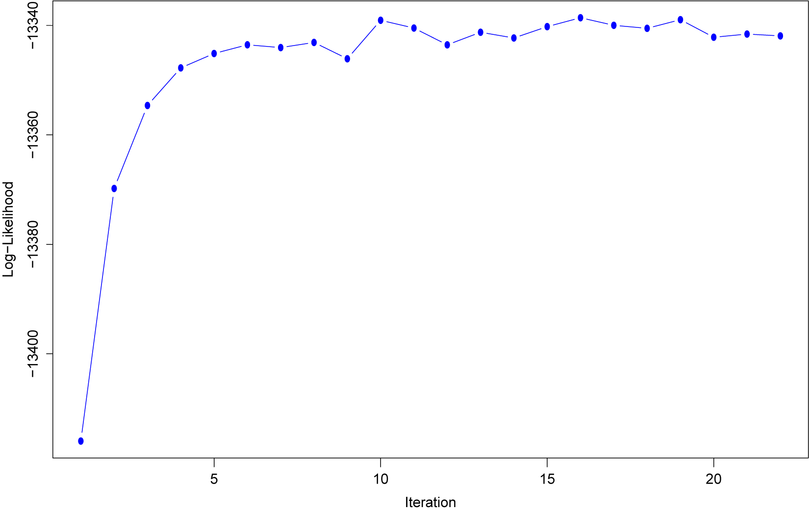
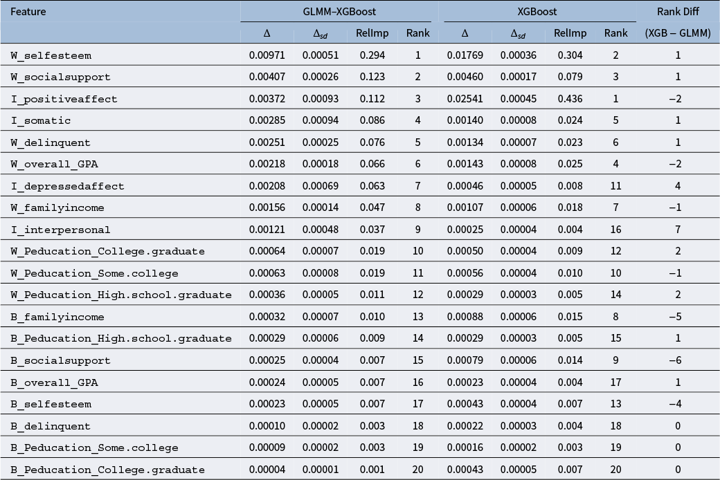
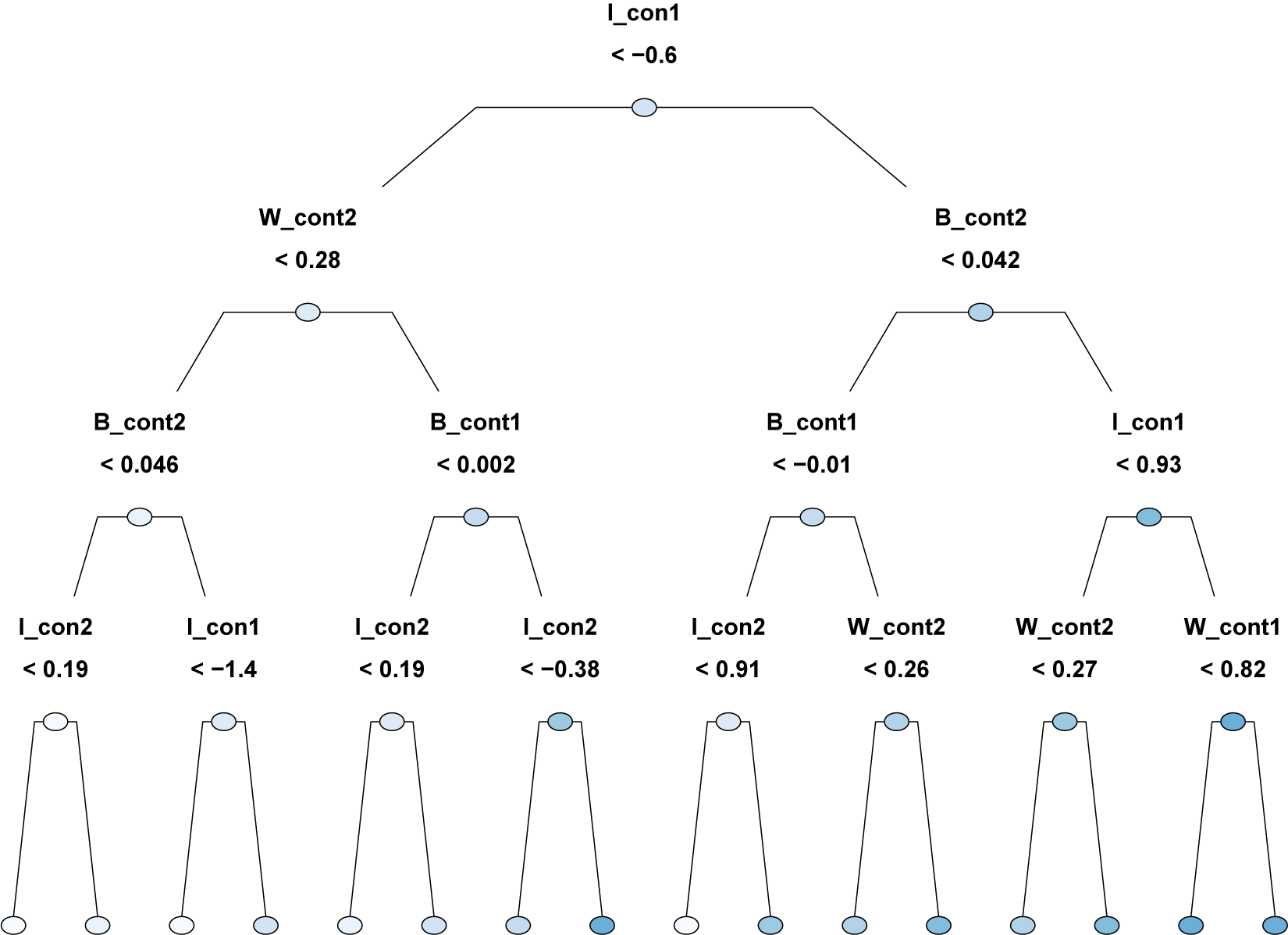
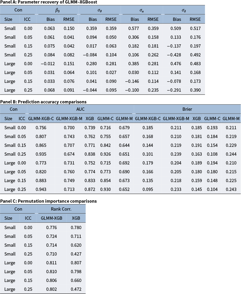
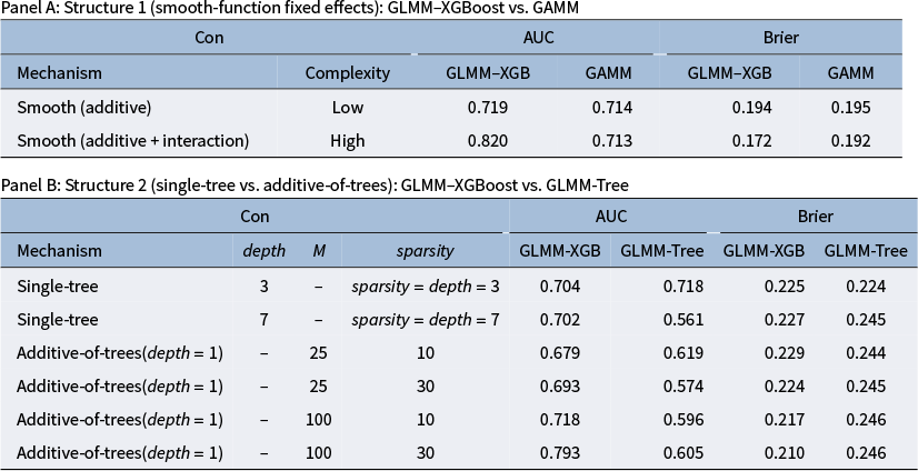
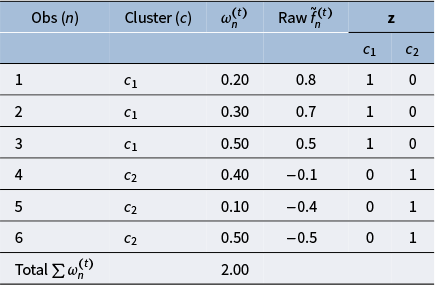
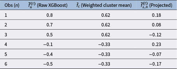
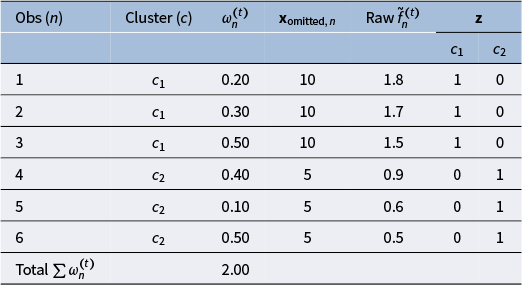
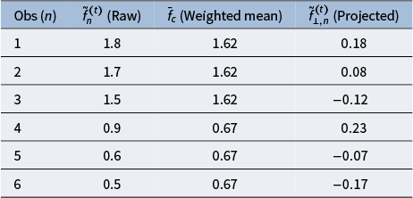


 Open access