





1 Introduction
Learning diagnosis, the process of identifying a learner’s strengths, weaknesses, and specific gaps in knowledge or skills, is a crucial component of effective learning, as formative assessment significantly improves academic performance (
$Effect\kern0.17em size=0.40, SE=0.06$
 ; Hattie, Reference Hattie2023, p. 333). Diagnostic classification models (DCMs; e.g., Rupp et al., Reference Rupp, Templin and Henson2010; von Davier & Lee, Reference von Davier and Lee2019), a family of statistical models, have been applied across various subjects to achieve this purpose. For example, Tatsuoka and Tatsuoka (Reference Tatsuoka and Tatsuoka1997) conducted a computer-adaptive diagnostic test for fraction–subtraction problems, demonstrating that remediation instructions based on diagnostic results improved attribute mastery. Similarly, mathematics data from the Trends in International Mathematics and Science Study (TIMSS) were analyzed using DCMs, revealing differences in attribute mastery status across countries (Lee et al., Reference Lee, Park and Taylan2011; Yamaguchi & Okada, Reference Yamaguchi and Okada2018). von Davier (Reference von Davier2008) applied a general diagnostic model (GDM) to analyze Test of English for International Communication (TOEIC) Internet-based testing (iBT) Reading and Listening data from two test forms, predicting mastery of reading skills (e.g., synthesizing and organizing) and listening skills (e.g., making inferences and connections) based on general abilities. Additionally, Chen and de la Torre (Reference Chen and de la Torre2014) analyzed the Programme for International Student Assessment (PISA) reading data using the generalized deterministic input noisy AND-gate (G-DINA; de la Torre, Reference de la Torre2011) model and its sub-models, demonstrating that main effect or saturated models might effectively fit the reading data. These examples highlight the versatility of DCMs in various test applications.
DCMs have been developed to extract information for formative assessment from test data. For example, Ayan and Çıkrıkçı (Reference Ayan and Çıkrıkçı2021) employed DCMs for math proficiency formative assessment, highlighting the main difference between DCMs and item response theory models (IRT models; e.g., Embretson & Reise, Reference Embretson and Reise2000; de Ayala, Reference de Ayala2013). IRT models assume a general uni- or multi-dimensional continuous latent trait to order individuals, facilitating the estimation of comparable test scores among test takers, even when different sets of test items are utilized. Horizontal equating or vertical scaling refers to the construction of a common scale from different sets of test items (e.g., Kolen & Brennan, Reference Kolen and Brennan2014). Therefore, IRT models are appropriate for high-stakes tests whose results have a substantial impact on test takers. DCMs, however, assume discrete latent traits such as the mastery or non-mastery of cognitive elements, termed attributes, to answer a test. These are formally introduced subsequently. DCMs estimate the mastery/non-mastery of latent traits for the following topics that students are required to learn. In other words, DCM results are employed for learning remediation or diagnosis of students’ current learning status.
DCMs are primarily used to diagnose whether specific cognitive elements, known as attributes, in a test are mastered by an individual. For example, Tatsuoka and Tatsuoka (Reference Tatsuoka and Tatsuoka1997) developed a remediation selection method based on Mahalanobis distance (Figure 2 in Tatsuoka & Tatsuoka, Reference Tatsuoka and Tatsuoka1997). In the fraction–subtraction example, students who fail to master attributes such as A5 (reducing the fraction part before getting the common denominator) and A8 (adjusting the whole number part), presented in Table 1 of Tatsuoka and Tatsuoka (Reference Tatsuoka and Tatsuoka1997), were recommended remediation for A5 owing to its proximity to the next attribute mastery pattern. However, this rule-space-based method does not apply to other types of DCMs.
Yamaguchi and Templin (Reference Yamaguchi and Templin2022c) proposed the use of Hasse diagrams to represent attribute mastery and corresponding observed test scores, demonstrating attributes that provide the largest score changes. Nevertheless, this method is closely related to a specific diagnostic test and lacks generalizability. Moreover, it does not identify the attributes most crucial for future learning. Prior achievement strongly influences subsequent achievement (
$Effect\kern0.17em size=0.73, SE=0.07$
 ; Hattie, Reference Hattie2023, p. 79), indicating that the importance of mastering specific attributes may vary for advancing learning. Using feedback based on DCMs, Zhan et al. (Reference Zhan, Man, Wind and Malone2022) provided a framework to combine eye-tracking and problem-solving behavior data to improve feedback and diagnosis about problem-solving skills. They reported empirical applicability and utility of the proposed framework.
The long-term implications of attribute mastery are of interest to teachers or educational psychologists. In particular, identifying cognitive abilities that can predict learning trajectories and determining methods through which these relationships can be effectively modeled are key considerations. Although DCMs can predict the importance of attributes on learning trajectories, a methodology to achieve this has not yet been proposed. To address this issue, we propose an integrated modeling approach for examining how diagnostic attribute mastery predicts subsequent learning trajectories.
Learning trajectories are typically represented by a latent growth curve model, or simply a growth curve (GC) model (Muthén & Muthén, Reference Muthén and Muthén2000; Oravecz & Muth, Reference Oravecz and Muth2018; Preacher et al., Reference Preacher, Wichman, MacCallum and Briggs2008). The GC model can be conceptualized as a multilevel model where the individual forms level 2, and measurement time constitutes level 1 (Raudenbush & Bryk, Reference Raudenbush and Bryk2002; Snijders & Bosker, Reference Snijders and Bosker2012). Using the structural equation model (SEM), the GC model can be formulated as a standard latent trait model (Newsom, Reference Newsom2015), which is a single-level model. Furthermore, the SEM can be extended to a multilevel model within educational measurement contexts, referred to as the multilevel SEM (Heck & Reid, Reference Heck, Reid and Hoyle2023; Pritikin et al., Reference Pritikin, Hunter, von Oertzen, Brick and Boker2017; Rabe-Hesketh et al., Reference Rabe-Hesketh, Skrondal and Pickles2004). Therefore, even the multilevel GC (MGC) model is a three-level model, the multilevel SEM can reduce it as a two-level model. More importantly, this approach enables the representation of group-level (e.g., school-level) trajectories, facilitating the separation of group- and individual-level changes. Consequently, purified versions of individual learning trajectories can be obtained using an MGC model.
Longitudinal growth has also been considered in the context of DCMs, as reported by Yamaguchi and Martinez (Reference Yamaguchi and Martinez2024). Major longitudinal DCMs include the hidden Markov model (HMM; e.g., Bishop, Reference Bishop2006) and latent transition model (LTM; e.g., Collins & Lanza, Reference Collins and Lanza2009) type DCMs. HMM- and LTM-type DCMs that model the transition probabilities of attribute masteries between time points are also major approaches. Madison and Bradshaw (Reference Madison and Bradshaw2018) proposed a latent transition DCM that is an extension of LTM and explained its estimation based on maximum likelihood with Mplus (Muthén & Muthén, Reference Muthén and Muthén1998–2017). Wang (Reference Wang2021) developed a penalized expectation–maximization estimation method. Using Bayesian approaches, Wang et al. (Reference Wang, Yang, Culpepper and Douglas2018) developed an HMM-type DCM to attribute-level mastery probability based on covariates and previous attribute mastery status, and its estimation was conducted using a Markov chain Monte Carlo (MCMC) method. Pan et al. (Reference Pan, Qin and Kingston2020) developed multivariate longitudinal DCMs that assumed GC models on attribute mastery probability and multivariate normal distribution on the intercept and slope factors. Zhang and Chang (Reference Zhang and Chang2020) employed a similar approach to that of Wang et al. (Reference Wang, Yang, Culpepper and Douglas2018) and incorporated random effects on measurement models from learning tools such as exercises, slides, videos, or games that affect attribute mastery.
Previous studies have several limitations. First, all tests are conducted over several time points using DCM as measurement models. In other words, they are interested in mastery status change in attributes over time. Therefore, the model is closed in DCMs. This implies that effective attributes that contribute to long-term improvements in learning cannot be determined using these models. Second, some studies have included random effects in their models. However, these effects are not caused by an individual-level effect, but rather by a group effect, which is naturally introduced by a multilevel data structure. Therefore, attribute masteries are not inherent to individuals because they contain a group-level effect. These models are not suitable for detecting attributes that are essential for long-term general proficiency in individual-level development. To address these issues, we investigate how diagnostic attribute mastery can be incorporated into multilevel growth modeling.
Furthermore, multilevel considerations are equally important for DCMs. Test performance is influenced not only by attribute mastery but also by group-level (e.g., school-level) differences. Construct irrelevant factors, such as group-level variations, may distort the relationship between cognitive elements and item responses. This is similar to the attenuation of correlation coefficients in classical test theory modeling. For example, compared with students at other types of schools, those at preparatory schools may exhibit higher correct item response probabilities even if mastering no attributes is required in the test. However, it may lead to an inappropriate diagnosis of attribute mastery because test answers contain a nuisance element. Therefore, such effects must be accounted for in the application of DCMs.
Multilevel DCMs can incorporate group-level effects as random intercepts within the standard multilevel models. However, previous DCMs have substantially overlooked this straightforward random effect. Higher-order models (de la Torre & Douglas, Reference de la Torre and Douglas2004; Ma, Reference Ma2022; Zhan, Jiao, Liao, et al., Reference Zhan, Jiao, Liao and Li2019) primarily consider continuous latent traits, similar to IRT models, for attributes. These approaches often utilize multilevel IRT models (Fox, Reference Fox2010; Fox & Glas, Reference Fox and Glas2001; Wang & Qiu, Reference Wang and Qiu2019) for higher-order models in DCMs (Huang, Reference Huang2017; Wang & Qiu, Reference Wang and Qiu2019). Only von Davier (Reference von Davier2007) focused on group effects on item response functions. However, major approaches are inconsistent with the categorical nature of latent abilities, which are considered discontinuous or categorical variables in DCMs. To address this issue, the present study directly incorporates group effects as a random effect.
We summarize the limitations of previous studies as follows: (1) previous DCM studies paid limited attention to the use of diagnostic information for predicting subsequent academic growth trajectories and (2) multilevel structures in diagnostic assessments and subsequent tests were not fully incorporated, even though ignoring such structures may lead to biased parameter estimation. To address these limitations, this study proposes an integrated modeling approach that accounts for random group effects for examining individual learning trajectories using a multilevel GC model. More specifically, we integrated existing DCM, SEM, and multilevel modeling approaches to formulate the proposed model. We also assessed the performance of the Bayesian estimation procedure for this model and demonstrated the risk of ignoring multilevel structures through Monte Carlo simulation studies. Furthermore, we conducted an empirical analysis using data from second to sixth grade in elementary schools. Importantly, we investigated how second-grade learning states predict subsequent developmental trajectories across later grades. Academic abilities, specifically mathematics/arithmetic skills, were measured using a vertically linked scale. At the second-grade level, students’ attribute mastery is estimated through a diagnostic test. From grades three to six, the GC model is applied to assess their progress. The formal specification of this setting is presented below.
Our contributions are as follows. First, the proposed model provides a perspective on how diagnostic information can be used: the use of attribute mastery profiles for examining subsequent learning trajectories. Traditionally, diagnostic information is employed for learning remediation. However, single-time-point diagnostic classification results do not indicate which attributes are important for later learning. The proposed model provides a possible modeling approach for this question. On the other hand, SEM and multilevel modeling approaches have generally not incorporated discrete latent mastery profiles for predictive purposes. Second, the proposed model combines DCMs, SEM, and multilevel models. This model can incorporate group-level variation as a random effect in DCMs and use diagnostic results to examine individual-level development separately from group-level change. Therefore, the proposed model allows examination of the long-term consequences of attribute mastery for subsequent academic development at the individual level while separating group-level effects. Without separating group- and individual-level growth, it is difficult to consider the effect of attribute mastery on later academic proficiency growth. This distinction has received limited attention in the DCM literature. Although the distinction between group-level and individual-level effects has received limited attention, it should be considered in educational testing settings. In addition, because individual developmental trajectories may not always be linear, the SEM-based formulation permits more flexible representations of longitudinal growth. To illustrate this point, we additionally illustrate a partially freely estimated slope-loading specification (Bollen & Curran, Reference Bollen and Curran2006, Chapter 4) within the current modeling setting.
The remainder of this article is structured as follows. Section 2 outlines the fundamental concepts of the random-effect DCM for the MGC (RDC–MGC) model. This section introduces the measurement component of the random-effect DCM (RDCM), the MGC model, and the structural model. The posterior distribution of the RDC–MGC is also formulated for Bayesian estimation, which is implemented through an MCMC method. Section 3 shows simulation studies to assess the appropriateness of the estimation method and consequences of ignoring multilevel structure. Section 4 describes the details of the dataset, which comprises a five-year longitudinal mathematical assessment in elementary schools. Moreover, it explains the Q-matrix and attributes defined in the mathematics test, along with a brief discussion of the vertical scaling procedure. Section 5 discusses implications of the proposed model and considers future applications and extensions of the model.
2 Formulation of random-effect diagnostic classification model for multilevel growth curve model
2.1 Overview of the RDC–MGC model
Figure 1 shows the path diagram of the RDC–MGC model, comprising three key components: the RDC measurement model, MGC, and structural model. The first component is the RDC measurement model, which includes two elements: the conventional attribute-related component and group random intercept. Studies have developed various DCMs, including the deterministic input noisy AND-gate model (DINA; de la Torre, Reference de la Torre2009; Junker & Sijtsma, Reference Junker and Sijtsma2001; Macready & Dayton, Reference Macready and Dayton1977; Maris, Reference Maris1999), deterministic input noisy OR-gate model (DINO; Templin & Henson, Reference Templin and Henson2006), noisy inputs deterministic AND-gate model (NIDA; Junker & Sijtsma, Reference Junker and Sijtsma2001), additive cognitive diagnostic model (A-CDM; de la Torre, Reference de la Torre2011), linear logistic model (LLM; Maris, Reference Maris1999), reduced reparametrized unified model (R-RUM; Hartz & Roussos, Reference Hartz and Roussos2008; Roussos et al., Reference Roussos, Dibello, Stout, Hartz, Henson, Templin, Leighton and Gierl2007), log-linear cognitive diagnostic model (LCDM; Henson et al., Reference Henson, Templin and Willse2009), G-DINA model Reference de la Torre2011, and GDM (von Davier, Reference von Davier2008). This study adopts the LCDM-based model because its formulation supports the integration of multilevel effects, similar to multilevel IRT models (Fox, Reference Fox2010; Huang & Wang, Reference Huang and Wang2014).
Path diagram of the proposed random-effects diagnostic classification model for multilevel growth curves.

Figure 1 Long description
The diagram is split horizontally by a dashed line.
Top Section: Group level model.
On the left, a circle labeled theta (Random effect) has arrows pointing to I sub (G) and S sub (G) (Latent growth curve model) via Gamma super (G). Theta also points down to person-level variables x sub 1 through x sub J. I sub (G) and S sub (G) have arrows pointing to a series of circles labeled mu sub 1, mu sub 2, mu sub 3, through mu sub T. Arrows from I sub (G) are labeled with 1. Arrows from S sub (G) are labeled with 0, 1, 2, through T. Small circles representing error terms point to each mu node.
Bottom Section: Person level model.
On the far left are square nodes x sub 1, x sub 2, x sub 3, through x sub J. These connect to a column of circles alpha sub 1, alpha sub 2, through alpha sub K (Diagnostic model) via a node labeled Lambda. These alpha nodes point to I sub (P) and S sub (P) (Structural model) via Gamma super (P). On the right, I sub (P) and S sub (P) (Latent growth curve model) point to square nodes y sub 1, y sub 2, y sub 3, through y sub T. Arrows from I sub (P) are labeled with 1. Arrows from S sub (P) are labeled with 0, 1, 2, through T. Vertical arrows also connect the group-level mu nodes to the corresponding person-level y nodes. Small circles representing error terms point to each y node.
The second component is the MGC model, a specialized form of multilevel SEM. It separates observed variables into group-level elements and individual-level components, enabling distinct modeling of these elements. Importantly, the individual growth trajectory derived from the MGC model excludes group-level changes, representing the inherent trajectory of the individual.
The final component is the structural model, which links attribute mastery to the individual intercept and slope of the GC, forming the individual-level model. This model explains how attribute mastery and its interactions account for individual differences in growth trajectories. Additionally, it captures the relationship between group-level differences which are modeled as a random intercept and group-level growth. Although this is a secondary focus, the model can be extended to include group-level covariates to account for variance in the intercept and slope at the group level. The details of these three components of the RDC–MGC model are presented in subsequent sections.
In our model, the multilevel growth model represents academic proficiency, which constitutes our outcome. We aim to construct a model representing the types of attributes that are significant for academic ability growth. Furthermore, we separated growth into two levels and therefore considered the growth between group and individual levels separately. The diagnostic assessment part, which is a single-point measurement, includes independent variables. However, previous DCMs do not consider the group-level baseline effect, which is a random effect. Moreover, they can distort attribute mastery. In other words, we considered the attribute masteries in previous single-level DCMs as the compound of individual attribute masteries and group-level proficiency. We explicitly formulated such random effects and attribute mastery effects that were fixed effects and usual DCM parameters. In summary, the random and fixed effects were assumed in the DCM measurement part. From the above discussion, the most interesting part of this model is the individual structural part that represents the relationship between purified attribute mastery and the growth of academic proficiency. The group-level structural part will be interesting if some group-level covariates can predict the level of growth in academic proficiency. A wider variety of empirical evaluations of group-level structures will be an important topic for future research.
The basic data structure in this model is that the diagnostic measurement is conducted at a single time point, and the attribute mastery patterns predict the growth trajectory. In this case, we assumed the research question to be about which kinds of attributes and their combinations are influential for subsequent learning. This is just an example of research. If we want to use longitudinal DCMs during the first period, we use such a transition as the diagnostic measurement part, and the final mastery pattern can be used as a predictor for the growth trajectory. In addition, we can simultaneously include both a diagnostic model and a usual IRT model in the first measurement phase if we prepare both a diagnostic test and an achievement test at that point. In this case, both continuous latent proficiency and attribute mastery are employed as predictors. Furthermore, the outcome growth model can be assumed for latent proficiency, which is a type of longitudinal IRT model (e.g., Wang & Nydick, Reference Wang and Nydick2020) or a second-order factor analysis model (e.g., Wickrama et al., Reference Wickrama, Lee, O'Neal and Lorenz2016). In this case, tests at different time points should include anchor items to ensure that the same continuous proficiency is being measured. In the current study, for the simplicity of the model, we employed estimated academic proficiency based on vertically scaled tests.
2.2 Measurement component of RDCMs
The RDCM can be expressed in various formulations, as multilevel latent class models can be specified in various ways (e.g., Henry & Muthén, Reference Henry and Muthén2010; Vermunt, Reference Vermunt and Stoltzenberg2003, Reference Vermunt2008). Therefore, RDCM assumes a two-stage sampling procedure for the diagnostic measurement, in which level two units such as schools are randomly sampled first, then the level one units such as students are randomly sampled. Additionally, as previously discussed, numerous DCMs have been developed. In this study, we adopted the LCDM formulation with a random effect. The LCDM defines the probability of a correct item response based on the attribute mastery pattern, model parameters, and Q-matrix.
First, we assume
$K\in \mathbb{N}$
 attributes for the test, where the subscript
$k\in \left\{1,2,\dots, K\right\}$
attributes for the test, where the subscript
$k\in \left\{1,2,\dots, K\right\}$
 represents the attribute index. Subsequently, the
$l\left(\in \left\{1,2,\dots, L={2}^K\right\}\right)$
represents the attribute index. Subsequently, the
$l\left(\in \left\{1,2,\dots, L={2}^K\right\}\right)$
 -th attribute mastery pattern is represented as a latent binary vector of length
$K$
-th attribute mastery pattern is represented as a latent binary vector of length
$K$
 :
${\boldsymbol{\unicode{x3b1}}}_l\in {\left\{0,1\right\}}^K.$
:
${\boldsymbol{\unicode{x3b1}}}_l\in {\left\{0,1\right\}}^K.$
 Its
$k$
Its
$k$
 -th element is
${\unicode{x3b1}}_{lk}\in \left\{0,1\right\}$
-th element is
${\unicode{x3b1}}_{lk}\in \left\{0,1\right\}$
 representing non-mastery (
$=0$
representing non-mastery (
$=0$
 ) and mastery (
$=1$
) and mastery (
$=1$
 ) of the attribute. For individual
$i\in \left\{1,2,\dots, I\in \mathbb{N}\right\}$
) of the attribute. For individual
$i\in \left\{1,2,\dots, I\in \mathbb{N}\right\}$
 , whose mastery status corresponds to
${\boldsymbol{\unicode{x3b1}}}_l$
, whose mastery status corresponds to
${\boldsymbol{\unicode{x3b1}}}_l$
 , we denote this as
${\boldsymbol{\unicode{x3b1}}}_i={\boldsymbol{\unicode{x3b1}}}_l$
, we denote this as
${\boldsymbol{\unicode{x3b1}}}_i={\boldsymbol{\unicode{x3b1}}}_l$
 . Based on the multilevel structure, individuals (level one unit) are exchangeable given a school (level two unit).
Furthermore,
${\boldsymbol{q}}_j\in {\left\{0,1\right\}}^K\backslash {\boldsymbol{0}}_K$
 , where
$j$
, where
$j$
 is an element of the set
$\left\{1,2,\dots, J\in \mathbb{N}\right\},$
is an element of the set
$\left\{1,2,\dots, J\in \mathbb{N}\right\},$
 and
${\boldsymbol{0}}_K$
and
${\boldsymbol{0}}_K$
 is the length
$K$
is the length
$K$
 of the zero vector, which is a
$q$
of the zero vector, which is a
$q$
 -vector. The
$k$
-vector. The
$k$
 -th element
${q}_{jk}\in \left\{0,1\right\}$
-th element
${q}_{jk}\in \left\{0,1\right\}$
 is set to 1 if the
$k$
is set to 1 if the
$k$
 -th attribute is measured by item
$j$
-th attribute is measured by item
$j$
 and 0 otherwise. Using these definitions, the probability of a correct response for individual
$i$
and 0 otherwise. Using these definitions, the probability of a correct response for individual
$i$
 belonging to the
$m\left(=\left\{1,2,\dots, M\in \mathbb{N}\right\}\right)$
belonging to the
$m\left(=\left\{1,2,\dots, M\in \mathbb{N}\right\}\right)$
 -th group on the test item
$j$
-th group on the test item
$j$
 is given by

where
${\boldsymbol{\unicode{x3bb}}}_j=\left\{{\unicode{x3bb}}_{j0},{\unicode{x3bb}}_{j1},\dots, {\lambda}_{j12\dots K}\right\}$
 and
and

The parameter
${\boldsymbol{\unicode{x3bb}}}_j$
 is a vector-fixed effect; therefore, it does not change over school and includes the intercept
${\unicode{x3bb}}_{j0}$
is a vector-fixed effect; therefore, it does not change over school and includes the intercept
${\unicode{x3bb}}_{j0}$
 , main effects of mastering individual attributes such as
${\unicode{x3bb}}_{jk}$
, main effects of mastering individual attributes such as
${\unicode{x3bb}}_{jk}$
 , and interaction effects among attributes, denoted as
${\unicode{x3bb}}_{j12\dots K}$
, and interaction effects among attributes, denoted as
${\unicode{x3bb}}_{j12\dots K}$
 . The parameter
${\unicode{x3bb}}_{j0}$
. The parameter
${\unicode{x3bb}}_{j0}$
 corresponds to the item response probability of all non-mastery patterns when the average group (i.e.,
${\unicode{x3b8}}_m=0$
corresponds to the item response probability of all non-mastery patterns when the average group (i.e.,
${\unicode{x3b8}}_m=0$
 ). Therefore, it determines the baseline item response probability. If the intercept is negative, set
${\unicode{x3b8}}_m=0$
). Therefore, it determines the baseline item response probability. If the intercept is negative, set
${\unicode{x3b8}}_m=0$
 ; the item response probability of the baseline is less than 0.5, which is desirable. The main effect
${\unicode{x3bb}}_{jk}$
; the item response probability of the baseline is less than 0.5, which is desirable. The main effect
${\unicode{x3bb}}_{jk}$
 denotes the increase in the logit of mastering
$k$
denotes the increase in the logit of mastering
$k$
 -th attribute. In DCMs, the main effect is positive because of the monotonicity constraint (e.g., Henson et al., Reference Henson, Templin and Willse2009; Yamaguchi & Templin, Reference Yamaguchi and Templin2022a). The interaction effect
${\unicode{x3bb}}_{jk{k}^{\prime }}$
-th attribute. In DCMs, the main effect is positive because of the monotonicity constraint (e.g., Henson et al., Reference Henson, Templin and Willse2009; Yamaguchi & Templin, Reference Yamaguchi and Templin2022a). The interaction effect
${\unicode{x3bb}}_{jk{k}^{\prime }}$
 determines the probability of an individual simultaneously mastering attributes
$k$
determines the probability of an individual simultaneously mastering attributes
$k$
 and
${k}^{\prime }$
and
${k}^{\prime }$
 . Similarly, the highest interaction term
${\unicode{x3bb}}_{j12\dots K}$
. Similarly, the highest interaction term
${\unicode{x3bb}}_{j12\dots K}$
 is the effect on item response probability when an individual masters all attributes required by the
$j$
is the effect on item response probability when an individual masters all attributes required by the
$j$
 -th item if
${\prod}_{k=1}^K{q}_{jk}=1$
-th item if
${\prod}_{k=1}^K{q}_{jk}=1$
 . A key feature of the RDCM is the random effect
${\unicode{x3b8}}_m$
. A key feature of the RDCM is the random effect
${\unicode{x3b8}}_m$
 , which is an element of an
$M$
, which is an element of an
$M$
 -length vector
$\boldsymbol{\unicode{x3b8}} \mathbf{\in}{\mathbb{R}}^M$
-length vector
$\boldsymbol{\unicode{x3b8}} \mathbf{\in}{\mathbb{R}}^M$
 , assumed to follow a normal distribution
$N\left(0,{\unicode{x3c3}}_{\unicode{x3b8}}^2\right).$
, assumed to follow a normal distribution
$N\left(0,{\unicode{x3c3}}_{\unicode{x3b8}}^2\right).$
 The random effect modifies the interpretation of the intercept
${\unicode{x3bb}}_{j0}$
The random effect modifies the interpretation of the intercept
${\unicode{x3bb}}_{j0}$
 , which represents the probability of a correct item response for individuals with no attribute mastery in an average group.
Furthermore, in the multilevel IRT model literature, such as Fox and Glas (Reference Fox and Glas2001, p. 283), it is indicated that the random intercept is defined as an expected school achievement when controlling other variables. Considering this interpretation, if the RDC–MGC includes covariates of the school or individuals, its random intercept leads to the expected group achievement. The simplest version is the no-covariate case, which is mainly employed in the empirical study, and the random intercept represents school differences in the diagnostic test. Furthermore, the diagnostic measurement models include attribute mastery status, and its intercepts represent the correct response probabilities of the all no-mastering pattern, which is the baseline. Therefore, the random intercept in the simplest version of the RDC–MGC model is the group difference of all the non-mastery patterns. This group difference may explain the guessing probability in the DCM.
Note that the random effect
${\unicode{x3b8}}_m$
 can formally be a uniform DIF factor. Basically, DIF systematically changes some item response functions caused by group differences, and its factor is represented as a fixed effect. Li and Wang (Reference Li and Wang2015) proposed a unified formulation of DIF in DCMs. Li and Wang (Reference Li and Wang2015, pp. 30–31) reported that using latent proficiencies as grouping factors can cause DIF. Further, Camilli (Reference Camilli and Brennan2006, p. 241) mentioned that DIF can be caused by secondary distribution. For numerous groups, the DIF term can be modified as a random effect in an item (Camilli, Reference Camilli and Brennan2006, pp. 242–243). Therefore, technically and formally, the group-level proficiency
${\unicode{x3b8}}_m$
can formally be a uniform DIF factor. Basically, DIF systematically changes some item response functions caused by group differences, and its factor is represented as a fixed effect. Li and Wang (Reference Li and Wang2015) proposed a unified formulation of DIF in DCMs. Li and Wang (Reference Li and Wang2015, pp. 30–31) reported that using latent proficiencies as grouping factors can cause DIF. Further, Camilli (Reference Camilli and Brennan2006, p. 241) mentioned that DIF can be caused by secondary distribution. For numerous groups, the DIF term can be modified as a random effect in an item (Camilli, Reference Camilli and Brennan2006, pp. 242–243). Therefore, technically and formally, the group-level proficiency
${\unicode{x3b8}}_m$
 is a special case of the DIF factor that affects the same difficulty shift on the all-test items.
However, the group-level factor
${\unicode{x3b8}}_m$
 and usual DIF factor exhibit certain differences. The DIF is assumed for each item, and the group difference of the intercepts can vary across items. Even when the DIF factor is a random effect, it is assumed for items that may be different among groups. In addition, in DIF consideration, the number of assumed groups is relatively small. The group-level factor
${\unicode{x3b8}}_m$
and usual DIF factor exhibit certain differences. The DIF is assumed for each item, and the group difference of the intercepts can vary across items. Even when the DIF factor is a random effect, it is assumed for items that may be different among groups. In addition, in DIF consideration, the number of assumed groups is relatively small. The group-level factor
${\unicode{x3b8}}_m$
 is shared for all items and serves as a common factor. Method factors may be similar to the group-level factor
${\unicode{x3b8}}_m$
is shared for all items and serves as a common factor. Method factors may be similar to the group-level factor
${\unicode{x3b8}}_m$
 , but they model correlations among sub-items caused by item traits. The random intercept in our study can be considered a group-level difference parameter, as mentioned and can predict the intercept and slope of the growth model part, which will be introduced subsequently, in the real-data analysis. From these points, the random effect may be a group-level proficiency rather than just the uniform DIF.
Note that, although the LCDM formulation is employed, the distribution of attribute mastery should be specified at the attribute mastery level, consistent with latent class formulations (Yamaguchi & Okada, Reference Yamaguchi and Okada2020; Yamaguchi & Templin, Reference Yamaguchi and Templin2022a, Reference Yamaguchi and Templin2022b). This implies that attribute mastery patterns are latent classes rather than a decomposition of each attribute mastery. For example, when the number of attributes is
${K=3}$
 ,
$L={2}^K={2}^3=8$
,
$L={2}^K={2}^3=8$
 attribute mastery patterns,
$\left(0,0,0\right),\left(0,0,1\right),\left(0,1,0\right),\dots, \left(1,1,1\right)$
attribute mastery patterns,
$\left(0,0,0\right),\left(0,0,1\right),\left(0,1,0\right),\dots, \left(1,1,1\right)$
 , were assumed. The eight attribute mastery patterns are followed by a categorical distribution. In this formulation, the attributes need not be independent. Specifically, we represent an individual
$i$
, were assumed. The eight attribute mastery patterns are followed by a categorical distribution. In this formulation, the attributes need not be independent. Specifically, we represent an individual
$i$
 in group
$m$
in group
$m$
 having a specific attribute mastery pattern
${\boldsymbol{\unicode{x3b1}}}_l$
having a specific attribute mastery pattern
${\boldsymbol{\unicode{x3b1}}}_l$
 as
$\mathcal{I}\left({\boldsymbol{\unicode{x3b1}}}_{im}={\boldsymbol{\unicode{x3b1}}}_l\right)$
as
$\mathcal{I}\left({\boldsymbol{\unicode{x3b1}}}_{im}={\boldsymbol{\unicode{x3b1}}}_l\right)$
 , which is an indicator function taking value 1 if its argument is true, and 0 otherwise, and its probability of taking value 1 is
${\unicode{x3c0}}_l$
, which is an indicator function taking value 1 if its argument is true, and 0 otherwise, and its probability of taking value 1 is
${\unicode{x3c0}}_l$
 , satisfying
${\sum}_l{\unicode{x3c0}}_l=1$
, satisfying
${\sum}_l{\unicode{x3c0}}_l=1$
 . Therefore, the probability distribution of
$\mathcal{I}\left({\boldsymbol{\unicode{x3b1}}}_{im}={\boldsymbol{\unicode{x3b1}}}_l\right)$
. Therefore, the probability distribution of
$\mathcal{I}\left({\boldsymbol{\unicode{x3b1}}}_{im}={\boldsymbol{\unicode{x3b1}}}_l\right)$
 is a categorical distribution:

Furthermore, we assume that the exchangeability of individuals results in the joint distribution of
$\mathcal{A}={\left\{{\boldsymbol{\unicode{x3b1}}}_{im}\right\}}_{i,m=1}^{I_m,M}$
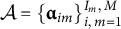 can be expressed as

From these assumptions, the joint distribution of data
$\mathrm{X}={\left\{{x}_{ijm}\right\}}_{i,j,m=1}^{I_m,J,M}$
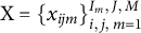 , latent attribute mastery pattern
$\mathcal{A}$
, latent attribute mastery pattern
$\mathcal{A}$
 , and group random effect
$\boldsymbol{\unicode{x3b8}}$
, and group random effect
$\boldsymbol{\unicode{x3b8}}$
 is given by

where
${\Lambda}_X={\left\{{\boldsymbol{\unicode{x3bb}}}_j\right\}}_{j=1}^J$
 . This will be employed subsequently.
2.3 Latent GC model component
We briefly outline the general notation for two-level SEM and then apply it to a two-level GC model. The general multilevel SEM has been extensively investigated in the literature (Depaoli, Reference Depaoli2021; Depaoli & Clifton, Reference Depaoli and Clifton2015; Heck & Reid, Reference Heck, Reid and Hoyle2023; Muthén, Reference Muthén1994; Rabe-Hesketh et al., Reference Rabe-Hesketh, Skrondal and Pickles2004). The two-level GC model decomposes the observed variable as follows:

where
${\boldsymbol{y}}_{im},{\boldsymbol{\unicode{x3b5}}}_{im}^{(P)},$
 and
${\boldsymbol{\unicode{x3b5}}}_m^{(G)}$
and
${\boldsymbol{\unicode{x3b5}}}_m^{(G)}$
 are the outcome vector of
$T$
are the outcome vector of
$T$
 time points and residual vectors for each level:
${\boldsymbol{y}}_{im}={\left({y}_{1 im},\dots, {y}_{tim},\dots, {y}_{Tim}\right)}^{\top }$
time points and residual vectors for each level:
${\boldsymbol{y}}_{im}={\left({y}_{1 im},\dots, {y}_{tim},\dots, {y}_{Tim}\right)}^{\top }$
 ,
${\boldsymbol{\unicode{x3b5}}}_{im}^{(P)}={\left({\unicode{x3b5}}_{1 im}^{(P)},\dots, {\unicode{x3b5}}_{tim}^{(P)},\dots, {\unicode{x3b5}}_{Tim}^{(P)}\right)}^{\top },{\boldsymbol{\unicode{x3b5}}}_m^{(G)}={\left({\unicode{x3b5}}_{1m}^{(G)},\dots, {\unicode{x3b5}}_{tm}^{(G)},\dots, {\unicode{x3b5}}_{Tm}^{(G)}\right)}^{\top }.$
,
${\boldsymbol{\unicode{x3b5}}}_{im}^{(P)}={\left({\unicode{x3b5}}_{1 im}^{(P)},\dots, {\unicode{x3b5}}_{tim}^{(P)},\dots, {\unicode{x3b5}}_{Tim}^{(P)}\right)}^{\top },{\boldsymbol{\unicode{x3b5}}}_m^{(G)}={\left({\unicode{x3b5}}_{1m}^{(G)},\dots, {\unicode{x3b5}}_{tm}^{(G)},\dots, {\unicode{x3b5}}_{Tm}^{(G)}\right)}^{\top }.$
 For example,
${\boldsymbol{y}}_{im}$
For example,
${\boldsymbol{y}}_{im}$
 contains the academic test scores of an individual
$i$
contains the academic test scores of an individual
$i$
 belonging to the
$m$
belonging to the
$m$
 -th school during elementary school period. Equation (6) indicates that such an individual academic score can be decomposed into the school effect part (group-level model) and the person’s own part (person-level model). Note that the residual term vectors
${\boldsymbol{\unicode{x3b5}}}_{im}^{(P)}$
-th school during elementary school period. Equation (6) indicates that such an individual academic score can be decomposed into the school effect part (group-level model) and the person’s own part (person-level model). Note that the residual term vectors
${\boldsymbol{\unicode{x3b5}}}_{im}^{(P)}$
 and
${\boldsymbol{\unicode{x3b5}}}_m^{(G)}$
and
${\boldsymbol{\unicode{x3b5}}}_m^{(G)}$
 are independent from another random variable such as
${\boldsymbol{y}}_{im}$
are independent from another random variable such as
${\boldsymbol{y}}_{im}$
 . However, within the vector, the elements of
${\boldsymbol{\unicode{x3b5}}}_{im}^{(P)}$
. However, within the vector, the elements of
${\boldsymbol{\unicode{x3b5}}}_{im}^{(P)}$
 or
${\boldsymbol{\unicode{x3b5}}}_m^{(G)}$
or
${\boldsymbol{\unicode{x3b5}}}_m^{(G)}$
 can be correlated just the same as usual longitudinal model assumptions. Therefore, for example, we can assume that
${\boldsymbol{\unicode{x3b5}}}_{im}^{(P)}$
can be correlated just the same as usual longitudinal model assumptions. Therefore, for example, we can assume that
${\boldsymbol{\unicode{x3b5}}}_{im}^{(P)}$
 or
${\boldsymbol{\unicode{x3b5}}}_m^{(G)}$
or
${\boldsymbol{\unicode{x3b5}}}_m^{(G)}$
 is generated from a multivariate normal distribution. However, for the simplicity of the model, we assume that the residuals independently follow different distributions which will be shown later.
Furthermore, consistent with the usual GC model, the latent variables represent the intercept and slope:
${\boldsymbol{\unicode{x3b7}}}_{im}^{(P)}={\left({I}_{im}^{(P)},{S}_{im}^{(P)}\right)}^{\top }$
 and
${\boldsymbol{\unicode{x3b7}}}_m^{(G)}={\left({I}_m^{(G)},{S}_m^{(G)}\right)}^{\top }$
and
${\boldsymbol{\unicode{x3b7}}}_m^{(G)}={\left({I}_m^{(G)},{S}_m^{(G)}\right)}^{\top }$
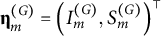 . The upper scripts “
$(P)$
. The upper scripts “
$(P)$
 ” and “
$(G)$
” and “
$(G)$
 ” represent person- and group-level variables, respectively. Therefore,
${\boldsymbol{\unicode{x3b7}}}_{im}^{(P)}$
” represent person- and group-level variables, respectively. Therefore,
${\boldsymbol{\unicode{x3b7}}}_{im}^{(P)}$
 and
${\boldsymbol{\unicode{x3b7}}}_m^{(G)}$
and
${\boldsymbol{\unicode{x3b7}}}_m^{(G)}$
 are the vectors of person-level intercept and slope of individual
$i$
are the vectors of person-level intercept and slope of individual
$i$
 in group
$m$
in group
$m$
 and group-level intercept and slope of group
$m$
and group-level intercept and slope of group
$m$
 , respectively. More intuitively,
${\boldsymbol{\unicode{x3b7}}}_m^{(G)}$
, respectively. More intuitively,
${\boldsymbol{\unicode{x3b7}}}_m^{(G)}$
 represents the
$m$
represents the
$m$
 -th school’s specific growth rate and the initial value of the academic performance, and
${\boldsymbol{\unicode{x3b7}}}_{im}^{(P)}$
-th school’s specific growth rate and the initial value of the academic performance, and
${\boldsymbol{\unicode{x3b7}}}_{im}^{(P)}$
 corresponds to the individual’s specific growth rate and initial status.
The covariance matrix of the intercept and slope can be represented as
${\Sigma}^{\left(\mathrm{P}\right)}$
 and
${\Sigma}^{\left(\mathrm{G}\right)}$
and
${\Sigma}^{\left(\mathrm{G}\right)}$
 , respectively. All the elements of the ground mean vector
${\boldsymbol{\unicode{x3bc}}}^{(Ground)}={\left({\unicode{x3bc}}_1^{(Ground)},\dots, {\unicode{x3bc}}_t^{(Ground)},\dots, {\unicode{x3bc}}_T^{(Ground)}\right)}^{\top}$
, respectively. All the elements of the ground mean vector
${\boldsymbol{\unicode{x3bc}}}^{(Ground)}={\left({\unicode{x3bc}}_1^{(Ground)},\dots, {\unicode{x3bc}}_t^{(Ground)},\dots, {\unicode{x3bc}}_T^{(Ground)}\right)}^{\top}$
 are fixed to zero for identifiability in this study. Therefore, we set
${\boldsymbol{\unicode{x3bc}}}^{(Ground)}={\boldsymbol{0}}_T$
are fixed to zero for identifiability in this study. Therefore, we set
${\boldsymbol{\unicode{x3bc}}}^{(Ground)}={\boldsymbol{0}}_T$
 and omitted this vector for simplicity. Furthermore, we assume a linear GC model for both levels; the time score matrix is
${\Lambda}_Y^{(P)}={\Lambda}_Y^{(G)}=\left(\begin{array}{cc}1& 0\\ {}1& 1\\ {}\vdots & \vdots \\ {}1& T\end{array}\right)$
and omitted this vector for simplicity. Furthermore, we assume a linear GC model for both levels; the time score matrix is
${\Lambda}_Y^{(P)}={\Lambda}_Y^{(G)}=\left(\begin{array}{cc}1& 0\\ {}1& 1\\ {}\vdots & \vdots \\ {}1& T\end{array}\right)$
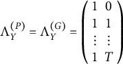 . Representing
${\boldsymbol{\unicode{x3bc}}}_m^{(G)}={\Lambda}_Y^{(G)}{\boldsymbol{\unicode{x3b7}}}_m^{(G)}+{\boldsymbol{\unicode{x3b5}}}_m^{(G)}={\left({\unicode{x3bc}}_{1m}^{(G)},\dots, {\unicode{x3bc}}_{tm}^{(G)},\dots, {\unicode{x3bc}}_{Tm}^{(G)}\right)}^{\top }$
. Representing
${\boldsymbol{\unicode{x3bc}}}_m^{(G)}={\Lambda}_Y^{(G)}{\boldsymbol{\unicode{x3b7}}}_m^{(G)}+{\boldsymbol{\unicode{x3b5}}}_m^{(G)}={\left({\unicode{x3bc}}_{1m}^{(G)},\dots, {\unicode{x3bc}}_{tm}^{(G)},\dots, {\unicode{x3bc}}_{Tm}^{(G)}\right)}^{\top }$
 , which is the
$m$
, which is the
$m$
 -th school’s average trajectory for the academic performance, the element wise person-level model is given by


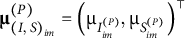
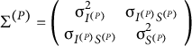
where the person-level mean vector and covariance matrix of the intercept and slope are
${\boldsymbol{\unicode{x3bc}}}_{{\left(I,S\right)}_{im}}^{(P)}={\left({\unicode{x3bc}}_{I_{im}^{(P)}},{\unicode{x3bc}}_{S_{im}^{(P)}}\right)}^{\top }$
 and
${\Sigma}^{(P)}=\left(\begin{array}{cc}{\unicode{x3c3}}_{I^{(P)}}^2& {\unicode{x3c3}}_{I^{(P)}{S}^{(P)}}\\ {}{\unicode{x3c3}}_{I^{(P)}{S}^{(P)}}& {\unicode{x3c3}}_{S^{(P)}}^2\end{array}\right)$
and
${\Sigma}^{(P)}=\left(\begin{array}{cc}{\unicode{x3c3}}_{I^{(P)}}^2& {\unicode{x3c3}}_{I^{(P)}{S}^{(P)}}\\ {}{\unicode{x3c3}}_{I^{(P)}{S}^{(P)}}& {\unicode{x3c3}}_{S^{(P)}}^2\end{array}\right)$
 , respectively. Here, the
$\mu$
, respectively. Here, the
$\mu$
 in the right-hand side of
${\mu}_{tm}$
in the right-hand side of
${\mu}_{tm}$
 is fixed to zero to identify the model. The
${I}_{im}^{(P)}+\left(t-1\right){S}_{im}^{(P)}$
is fixed to zero to identify the model. The
${I}_{im}^{(P)}+\left(t-1\right){S}_{im}^{(P)}$
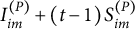 part in Equation (7) represents the deviation of the individual
$i$
part in Equation (7) represents the deviation of the individual
$i$
 from
${\unicode{x3bc}}_{tm}^{(G)}$
from
${\unicode{x3bc}}_{tm}^{(G)}$
 , and this is the individual-level average score at time point
$t$
, and this is the individual-level average score at time point
$t$
 after controlling group effect
${\unicode{x3bc}}_{tm}^{(G)}$
after controlling group effect
${\unicode{x3bc}}_{tm}^{(G)}$
 . The mean vector
${\boldsymbol{\unicode{x3bc}}}_{{\left(I,S\right)}_{im}}^{(P)}$
. The mean vector
${\boldsymbol{\unicode{x3bc}}}_{{\left(I,S\right)}_{im}}^{(P)}$
 is modeled by attribute mastery later, and representing growth rate and initial academic performance are different among individuals. In addition,
${\Sigma}^{(P)}$
is modeled by attribute mastery later, and representing growth rate and initial academic performance are different among individuals. In addition,
${\Sigma}^{(P)}$
 controls the amount of variation of the initial values and slopes among individuals and relationship between the intercept and slope. If
${\unicode{x3c3}}_{I^{(P)}{S}^{(P)}}$
controls the amount of variation of the initial values and slopes among individuals and relationship between the intercept and slope. If
${\unicode{x3c3}}_{I^{(P)}{S}^{(P)}}$
 is a positive value, the individual achieved high initial academic performance and tended to extend his/her academic performance faster.
Similarly, the group-level GC model is analogous to the person-level model:


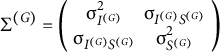
where the group-level mean vector and covariance matrix of the intercept and slope are
${\boldsymbol{\unicode{x3bc}}}_{{\left(I,S\right)}_m}^{(G)}={\left({\unicode{x3bc}}_{I_m^{(G)}},{\unicode{x3bc}}_{S_m^{(G)}}\right)}^{\top }$
 and
${\Sigma}^{(G)}=\left(\begin{array}{cc}{\unicode{x3c3}}_{I^{(G)}}^2& {\unicode{x3c3}}_{I^{(G)}{S}^{(G)}}\\ {}{\unicode{x3c3}}_{I^{(G)}{S}^{(G)}}& {\unicode{x3c3}}_{S^{(G)}}^2\end{array}\right)$
and
${\Sigma}^{(G)}=\left(\begin{array}{cc}{\unicode{x3c3}}_{I^{(G)}}^2& {\unicode{x3c3}}_{I^{(G)}{S}^{(G)}}\\ {}{\unicode{x3c3}}_{I^{(G)}{S}^{(G)}}& {\unicode{x3c3}}_{S^{(G)}}^2\end{array}\right)$
 , respectively. The interpretation of the group-level model is the same as the usual GC model.
For Bayesian analysis, the conditional likelihood, given the group-level score
${\boldsymbol{\unicode{x3bc}}}_Y^{(G)}={\left\{{\unicode{x3bc}}_{tm}^{(G)}\right\}}_{t,m=1}^{T,M}$
 and other person-level parameters, is expressed as where

$Y={\left\{{y}_{tim}\right\}}_{t,i,m=1}^{T,I_m,M}$
 and
${\boldsymbol{\unicode{x3c3}}}_{\unicode{x3b5}^{(P)}}^2={\left\{{\unicode{x3c3}}_{\unicode{x3B5}_{tm}^{(P)}}^2\right\}}_{t,m=1}^{T,M}$
and
${\boldsymbol{\unicode{x3c3}}}_{\unicode{x3b5}^{(P)}}^2={\left\{{\unicode{x3c3}}_{\unicode{x3B5}_{tm}^{(P)}}^2\right\}}_{t,m=1}^{T,M}$
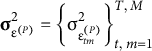 . Similarly, the conditional distribution of the group-level score
${\boldsymbol{\unicode{x3bc}}}_Y^{(G)}$
. Similarly, the conditional distribution of the group-level score
${\boldsymbol{\unicode{x3bc}}}_Y^{(G)}$
 , given the group-level parameters, is

where
${\boldsymbol{\unicode{x3c3}}}_{\unicode{x3b5}^{(G)}}^2=\left\{{\unicode{x3c3}}_{\unicode{x3B5}_1^{(G)}}^2,\dots, {\unicode{x3c3}}_{\unicode{x3B5}_T^{(G)}}^2\right\}$
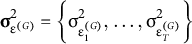 . Combining the expressions of the aforementioned two conditional likelihoods, the joint distribution of observed data and latent group-level score is given by

The joint and prior distributions, which will be introduced subsequently, are used to derive the posterior distribution of the model parameters.
2.4 Structural model component
The structural model represents the relationship between attribute mastery and the intercept and slope parameters in the person-level model. The person-level structural models are expressed as follows:


where the regression coefficients
${\Gamma}_I^{(P)}=\left\{{\unicode{x3b3}}_{I0}^{(P)},{\unicode{x3b3}}_{I1}^{(P)},\dots, {\unicode{x3b3}}_{I12\dots K}^{(P)}\right\}$
 and
${\Gamma}_S^{(P)}=\left\{{\unicode{x3b3}}_{S0}^{(P)},{\unicode{x3b3}}_{S1}^{(P)},\dots, {\unicode{x3b3}}_{S12\dots K}^{(P)}\right\}$
and
${\Gamma}_S^{(P)}=\left\{{\unicode{x3b3}}_{S0}^{(P)},{\unicode{x3b3}}_{S1}^{(P)},\dots, {\unicode{x3b3}}_{S12\dots K}^{(P)}\right\}$
 represent the mastery and interaction effects on the intercept and slope, respectively. Similar to the DCM measurement model, the person-level intercept on the growth model slope is
${\unicode{x3b3}}_{S0}^{(P)}$
represent the mastery and interaction effects on the intercept and slope, respectively. Similar to the DCM measurement model, the person-level intercept on the growth model slope is
${\unicode{x3b3}}_{S0}^{(P)}$
 , and it is an average slope value of all non-mastering groups. In addition, the person-level main effect of the first attribute on the growth model slope is
${\unicode{x3b3}}_{I1}^{(P)}$
, and it is an average slope value of all non-mastering groups. In addition, the person-level main effect of the first attribute on the growth model slope is
${\unicode{x3b3}}_{I1}^{(P)}$
 . This implies a difference in the growth speed between the non-mastering group and mastering first group. The person-level interaction on the growth model slope,
${\unicode{x3b3}}_{I12\dots K}^{(P)}$
. This implies a difference in the growth speed between the non-mastering group and mastering first group. The person-level interaction on the growth model slope,
${\unicode{x3b3}}_{I12\dots K}^{(P)}$
 , represents the effect of mastering all attributes measured in the test.
${\Gamma}_I^{(P)}$
, represents the effect of mastering all attributes measured in the test.
${\Gamma}_I^{(P)}$
 represents the effects of person-level attribute mastery on the growth intercept factor. The growth intercept factor is the initial academic proficiency level. Therefore,
${\Gamma}_I^{(P)}$
represents the effects of person-level attribute mastery on the growth intercept factor. The growth intercept factor is the initial academic proficiency level. Therefore,
${\Gamma}_I^{(P)}$
 represents how attribute masteries predict the initial academic proficiency level.
The random effect
$\unicode{x3b8}$
 and group-level growth are represented as follows:


Note that, if some group-level covariates are known, we can use them to explain group-level growth in Equations (14) and (15). The group-level effects are
${\unicode{x3b3}}_{\mathrm{I}}^{\left(\mathrm{G}\right)}$
 and
${\unicode{x3b3}}_{\mathrm{S}}^{\left(\mathrm{G}\right)}$
and
${\unicode{x3b3}}_{\mathrm{S}}^{\left(\mathrm{G}\right)}$
 , which represent the average change in the group-level intercept and slope factors by one-unit increase in the group-level random effect (e.g., group-level test answering skills), respectively. Using the above parameters, the joint distribution given in Equation (11) can be modified as

2.5 Full conditional distribution and estimation
To employ the Bayesian estimation method, we must specify priors for the model parameters. The mixing parameter
$\boldsymbol{\unicode{x3c0}}$
 follows a Dirichlet distribution with parameter
$\boldsymbol{\unicode{x3b4}}$
follows a Dirichlet distribution with parameter
$\boldsymbol{\unicode{x3b4}}$
 , and the LCDM parameters follow the normal distributions:
$\boldsymbol{\unicode{x3c0}} \sim Dir\left(\boldsymbol{\unicode{x3b4}} \right)$
, and the LCDM parameters follow the normal distributions:
$\boldsymbol{\unicode{x3c0}} \sim Dir\left(\boldsymbol{\unicode{x3b4}} \right)$
 and
$\unicode{x3bb} \sim N\left({\unicode{x3bc}}_{\unicode{x3bb}},{\unicode{x3c3}}_{\unicode{x3bb}}^2\right)$
and
$\unicode{x3bb} \sim N\left({\unicode{x3bc}}_{\unicode{x3bb}},{\unicode{x3c3}}_{\unicode{x3bb}}^2\right)$
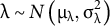 . The main effects should be positive; hence, we impose constraints on the prior distribution (Zhan, Jiao, Man, et al., Reference Zhan, Jiao, Man and Wang2019). The prior for the variance parameter of the random effect
${\unicode{x3b8}}_m$
. The main effects should be positive; hence, we impose constraints on the prior distribution (Zhan, Jiao, Man, et al., Reference Zhan, Jiao, Man and Wang2019). The prior for the variance parameter of the random effect
${\unicode{x3b8}}_m$
 is expressed as
${\unicode{x3c3}}_{\unicode{x3b8}}^2$
is expressed as
${\unicode{x3c3}}_{\unicode{x3b8}}^2$
 , which independently and identically follows an inverse gamma distribution:
${\unicode{x3c3}}_{\unicode{x3b8}}^2\sim IG\left(a,b\right)$
, which independently and identically follows an inverse gamma distribution:
${\unicode{x3c3}}_{\unicode{x3b8}}^2\sim IG\left(a,b\right)$
 . Combining the above prior settings with the conditional complete likelihood expressed in Equation (5), the joint distribution of the RDCM part can be expressed as follows:


where the priors are expressed by omitting their parameters, such as
$P\left(\boldsymbol{\unicode{x3c0}} \right)$
 , for notational simplicity.
Next, we set priors for the MGC model and structural part. The gamma parameters
${\boldsymbol{\Gamma} =\left\{{\Gamma}_I^{(P)},{\Gamma}_S^{(P)},{\unicode{x3b3}}_I^{(G)},{\unicode{x3b3}}_S^{(G)}\right\}}$
 are separately assumed to follow normal distributions. The priors for the MGC can be referenced from the Bayesian GC model (Depaoli & Clifton, Reference Depaoli and Clifton2015; Oravecz & Muth, Reference Oravecz and Muth2018). Measurement error variances, such as
${\unicode{x3c3}}_{\unicode{x3B5}_t^{(G)}}^2$
are separately assumed to follow normal distributions. The priors for the MGC can be referenced from the Bayesian GC model (Depaoli & Clifton, Reference Depaoli and Clifton2015; Oravecz & Muth, Reference Oravecz and Muth2018). Measurement error variances, such as
${\unicode{x3c3}}_{\unicode{x3B5}_t^{(G)}}^2$
 or
${\unicode{x3c3}}_{\unicode{x3B5}_{tm}^{(P)}}^2$
or
${\unicode{x3c3}}_{\unicode{x3B5}_{tm}^{(P)}}^2$
 , are again assumed to follow inverse gamma distributions. The covariance matrices for the intercept and slope
${\Sigma}^{(P)}$
, are again assumed to follow inverse gamma distributions. The covariance matrices for the intercept and slope
${\Sigma}^{(P)}$
 and
${\Sigma}^{(G)}$
and
${\Sigma}^{(G)}$
 are assumed to be generated from an inverse Wishart distribution:
${\Sigma}^{(P)}\sim IW\left({\Psi}^{(P)},{\unicode{x3bd}}^{(P)}\right)$
are assumed to be generated from an inverse Wishart distribution:
${\Sigma}^{(P)}\sim IW\left({\Psi}^{(P)},{\unicode{x3bd}}^{(P)}\right)$
 and
${\Sigma}^{(G)}\sim IW\left({\Psi}^{(G)},{\unicode{x3bd}}^{(G)}\right)$
and
${\Sigma}^{(G)}\sim IW\left({\Psi}^{(G)},{\unicode{x3bd}}^{(G)}\right)$
 , respectively, where
${\Psi}^{(P)}$
, respectively, where
${\Psi}^{(P)}$
 and
${\Psi}^{(G)}$
and
${\Psi}^{(G)}$
 are parameter matrices, and
${\unicode{x3bd}}^{(P)}$
are parameter matrices, and
${\unicode{x3bd}}^{(P)}$
 and
${\unicode{x3bd}}^{(G)}$
and
${\unicode{x3bd}}^{(G)}$
 are the degrees of freedom. Assuming the above priors and the conditional distribution expressed in Equation (11), the conditional distribution, given attribute mastery and random effects, is expressed as

Finally, from the above joint and conditional distributions, the joint distribution of data and parameters can be expressed as

3 Simulation study 1
We verified parameter recoveries (bias), parameter estimation variability (root mean square error: RMSE), and coverage of equal-tailed posterior credible intervals (95% CI coverage) using the Bayesian estimation procedure for the proposed RDC–MGC model in various settings. Attribute recoveries were also evaluated using attribute-level agreement ratio (AAR) and pattern-level agreement ratio (PAR). Furthermore, we assessed the effects on parameter recovery by ignoring multilevel structures. Applying a single-level version of the DCM with a single growth model under the RDC–MGC model data-generating system can provide biased, unstable estimations, and low coverage probabilities. Instead, considering a multilevel structure (e.g., RDC–MGC model) can recover true parameter values and achieve nominal coverage probabilities.
3.1 Simulation setting
The RDC–MGC model has various parameters or segments that can be manipulated. We manipulated three crucial factors: sample size, item quality of diagnostic measurement, and strength of the structural model. We assumed conditions of 200 and 1,000 sample sizes. In the 200 sample size condition, 10 schools (
$M=10$
 ) and 20 individuals were sampled from each school. This condition represented tracking a few individuals. Similarly, the 1,000 sample-size condition contained 25 schools (
$M=25$
) and 20 individuals were sampled from each school. This condition represented tracking a few individuals. Similarly, the 1,000 sample-size condition contained 25 schools (
$M=25$
 ) and 40 individuals, that is, approximately one class was sampled from each school. This condition indicates a relatively large-scale educational study, such as our real-data example.
The second factor was the item quality of the diagnostic measurement. High- and low-quality items were assumed, with the former exhibiting relatively stronger disclination power of attribute mastery patterns than the latter. According to Madison and Bradshaw (Reference Madison and Bradshaw2018, p. 917), LCDM item parameters were set to high/low-quality items, and the values were changed for the complexity of the item. The Q-matrix employed in this simulation is presented in Table 1, which has three attributes and nine simple structure items (items 1–9), nine middle complex items requiring two attributes (items 10–18), and two complex items measuring three attributes (items 19 and 20). In the condition of high-quality items, simple items had an intercept
${\unicode{x3bb}}_0=-2$
 and a main effect
${\unicode{x3bb}}_1=3$
and a main effect
${\unicode{x3bb}}_1=3$
 . The middle complex items had an intercept
${\unicode{x3bb}}_0=-2$
. The middle complex items had an intercept
${\unicode{x3bb}}_0=-2$
 , two main effects
${\unicode{x3bb}}_1=2$
, two main effects
${\unicode{x3bb}}_1=2$
 , and a first-order interaction
${\unicode{x3bb}}_2=1$
, and a first-order interaction
${\unicode{x3bb}}_2=1$
 . Finally, the two complex items had an intercept
${\unicode{x3bb}}_0=-3$
. Finally, the two complex items had an intercept
${\unicode{x3bb}}_0=-3$
 , three main effects
${\unicode{x3bb}}_1=1$
, three main effects
${\unicode{x3bb}}_1=1$
 , three first-order interactions
${\unicode{x3bb}}_2=0.5$
, three first-order interactions
${\unicode{x3bb}}_2=0.5$
 , and one second-order interaction
${\unicode{x3bb}}_3=1$
, and one second-order interaction
${\unicode{x3bb}}_3=1$
 . Low-quality items had half the parameter values as the high-quality items. For example, the simple items had an intercept
${\unicode{x3bb}}_0=-1$
. Low-quality items had half the parameter values as the high-quality items. For example, the simple items had an intercept
${\unicode{x3bb}}_0=-1$
 and a main effect
${\unicode{x3bb}}_1=1.5$
and a main effect
${\unicode{x3bb}}_1=1.5$
 .
.
Q-matrix for the first simulation study

Table 1 Long description
The table consists of four columns: Item, and Attributes 1, 2, and 3.
* Items 1, 4, and 7: Attribute 1 is 1; Attributes 2 and 3 are 0.
* Items 2, 5, and 8: Attribute 2 is 1; Attributes 1 and 3 are 0.
* Items 3, 6, and 9: Attribute 3 is 1; Attributes 1 and 2 are 0.
* Items 10, 13, and 16: Attributes 1 and 2 are 1; Attribute 3 is 0.
* Items 11, 14, and 17: Attributes 1 and 3 are 1; Attribute 2 is 0.
* Items 12, 15, and 18: Attributes 2 and 3 are 1; Attribute 1 is 0.
* Items 19 and 20: All three attributes are 1.
The last manipulation factor was the structural parameter strength, classified as strong or weak. The values were considered based on the results of the following real data. In the condition of the strong structural parameter, the main effects of the intercept were set to
$\left({\unicode{x3b3}}_{I1}^{(P)},{\unicode{x3b3}}_{I2}^{(P)},{\unicode{x3b3}}_{I3}^{(P)}\right)=\left(\mathrm{0.8,1},1.2\right)$
 . The interaction parameters were generated from the main effects
$\left({\unicode{x3b3}}_{I12}^{(P)},{\unicode{x3b3}}_{I13}^{(P)},{\unicode{x3b3}}_{I23}^{(P)}\right)=0.7\times \left({\unicode{x3b3}}_{I1}^{(P)}\times {\unicode{x3b3}}_{I2}^{(P)},{\unicode{x3b3}}_{I1}^{(P)}\times {\unicode{x3b3}}_{I3}^{(P)},{\unicode{x3b3}}_{I2}^{(P)}\times {\unicode{x3b3}}_{I3}^{(P)}\right)$
. The interaction parameters were generated from the main effects
$\left({\unicode{x3b3}}_{I12}^{(P)},{\unicode{x3b3}}_{I13}^{(P)},{\unicode{x3b3}}_{I23}^{(P)}\right)=0.7\times \left({\unicode{x3b3}}_{I1}^{(P)}\times {\unicode{x3b3}}_{I2}^{(P)},{\unicode{x3b3}}_{I1}^{(P)}\times {\unicode{x3b3}}_{I3}^{(P)},{\unicode{x3b3}}_{I2}^{(P)}\times {\unicode{x3b3}}_{I3}^{(P)}\right)$
 . The second-order interaction was determined by
${\unicode{x3b3}}_{I123}^{(P)}=0.7\times {\prod}_k{\unicode{x3b3}}_{Ik}^{(P)}.$
. The second-order interaction was determined by
${\unicode{x3b3}}_{I123}^{(P)}=0.7\times {\prod}_k{\unicode{x3b3}}_{Ik}^{(P)}.$
 The effect on the slope parameters
${\unicode{x3b3}}_S^{(P)}$
The effect on the slope parameters
${\unicode{x3b3}}_S^{(P)}$
 was half of the corresponding
${\unicode{x3b3}}_I^{(P)}$
was half of the corresponding
${\unicode{x3b3}}_I^{(P)}$
 . For example, the main effects on the slope were
$\left({\unicode{x3b3}}_{P1}^{(P)},{\unicode{x3b3}}_{P2}^{(P)},{\unicode{x3b3}}_{P3}^{(P)}\right)=0.5\times \left({\unicode{x3b3}}_{I1}^{(P)},{\unicode{x3b3}}_{I2}^{(P)},{\unicode{x3b3}}_{I3}^{(P)}\right)=\left(\mathrm{0.4,0.5,0.6}\right)$
. For example, the main effects on the slope were
$\left({\unicode{x3b3}}_{P1}^{(P)},{\unicode{x3b3}}_{P2}^{(P)},{\unicode{x3b3}}_{P3}^{(P)}\right)=0.5\times \left({\unicode{x3b3}}_{I1}^{(P)},{\unicode{x3b3}}_{I2}^{(P)},{\unicode{x3b3}}_{I3}^{(P)}\right)=\left(\mathrm{0.4,0.5,0.6}\right)$
 . The weak structural parameter assumed a quarter of the main effects of the intercept in the strong condition, and the same interaction-generating procedures were applied. These values were slightly arbitrary; therefore, various situations should be considered in future studies. The level two structural parameters
${\unicode{x3b3}}_I^{(G)}$
. The weak structural parameter assumed a quarter of the main effects of the intercept in the strong condition, and the same interaction-generating procedures were applied. These values were slightly arbitrary; therefore, various situations should be considered in future studies. The level two structural parameters
${\unicode{x3b3}}_I^{(G)}$
 and
${\unicode{x3b3}}_S^{(G)}$
and
${\unicode{x3b3}}_S^{(G)}$
 were set to
$-$
were set to
$-$
 2 and 1, respectively, in all conditions to maintain the simplicity of the simulation.
We set variance-related parameter values to real-data results. First, the variance of the random effect
${\unicode{x3b8}}_m$
 was
${\unicode{x3c3}}_{\unicode{x3b8}}^2=1.5$
was
${\unicode{x3c3}}_{\unicode{x3b8}}^2=1.5$
 . The variance–covariance matrices were
${\Sigma}^{(P)}=\left(\begin{array}{cc}{0.4}^2& 0.2\times 0.4\times 0.2\\ {}0.2\times 0.4\times 0.2& {0.2}^2\end{array}\right)$
. The variance–covariance matrices were
${\Sigma}^{(P)}=\left(\begin{array}{cc}{0.4}^2& 0.2\times 0.4\times 0.2\\ {}0.2\times 0.4\times 0.2& {0.2}^2\end{array}\right)$
 and
${\Sigma}^{(G)}=\left(\begin{array}{cc}{0.35}^2& 0.1\times {0.35}^2\\ {}0.1\times {0.35}^2& {0.35}^2\end{array}\right)$
and
${\Sigma}^{(G)}=\left(\begin{array}{cc}{0.35}^2& 0.1\times {0.35}^2\\ {}0.1\times {0.35}^2& {0.35}^2\end{array}\right)$
 , with 0.2 and 0.1 correlations for person and group levels, respectively. The person-level residual parameters
${\unicode{x3c3}}_{\unicode{x3B5}_t^{(P)}}^2$
, with 0.2 and 0.1 correlations for person and group levels, respectively. The person-level residual parameters
${\unicode{x3c3}}_{\unicode{x3B5}_t^{(P)}}^2$
 were all set to 0.2, and group-level residual variance
${\unicode{x3c3}}_{\unicode{x3B5}_t^{(G)}}^2$
were all set to 0.2, and group-level residual variance
${\unicode{x3c3}}_{\unicode{x3B5}_t^{(G)}}^2$
 was set to 0.1. We assumed a four-time point that was the same as the real-data analysis.
Using the above parameters, we generated 50 simulated data sets for each condition. Individuals’ attributes were generated using the modified procedures of Chiu et al. (Reference Chiu, Douglas and Li2009) or Yamaguchi and Martinez (Reference Yamaguchi and Martinez2024). Continuous attributes were first generated using a multivariate normal distribution with zero means and a correlation matrix with 0.4 values, and if the value exceeded 0, the attribute was considered mastered. The mixing parameters
$\boldsymbol{\unicode{x3c0}}$
 of the true attribute mastery pattern were calculated based on the distribution assumption.
For the same dataset, the RDC–MGC model and single-level version of the model, which did not include a random effect
${\unicode{x3b8}}_m$
 and the group-level growth model, were applied. Therefore, the single-level model did not have a group-level structural parameter. We considered the RDC–MGC and single-level models as the two- and single-level models to emphasize the differences between the models.
In the estimation, we assumed 2 chains and 20 thinning intervals. To determine the number of iterations, we conducted preliminary runs of the MCMC procedures. As a result, the MCMC iteration number was 20,000, which was generally enough for the convergence of the MCMC iteration, and the first 10,000 samples were discarded during the burn-in period. Prior settings are shown in the simulation script available on the OSF site: https://osf.io/gpztw.
Posterior means were employed for point estimates. For each parameter, such as
${\unicode{x3bb}}_{j0}$
 , we calculated
$\mathrm{Abs}.{\mathrm{Bias}}_{\unicode{x3BB}_{j0}}=\frac{1}{50}{\sum}_{n=1}^{50}\mid {\widehat{\unicode{x3bb}}}_{j0,n}-{\unicode{x3bb}}_{j0}^{\mathrm{True}}\mid$
, we calculated
$\mathrm{Abs}.{\mathrm{Bias}}_{\unicode{x3BB}_{j0}}=\frac{1}{50}{\sum}_{n=1}^{50}\mid {\widehat{\unicode{x3bb}}}_{j0,n}-{\unicode{x3bb}}_{j0}^{\mathrm{True}}\mid$
 ,
${\mathrm{RMSE}}_{\lambda_{j0}}=\sqrt{\frac{1}{50}{\sum}_{n=1}^{50}{\left({\widehat{\unicode{x3bb}}}_{j0,n}-{\unicode{x3bb}}_{j0}^{\mathrm{True}}\right)}^2}$
,
${\mathrm{RMSE}}_{\lambda_{j0}}=\sqrt{\frac{1}{50}{\sum}_{n=1}^{50}{\left({\widehat{\unicode{x3bb}}}_{j0,n}-{\unicode{x3bb}}_{j0}^{\mathrm{True}}\right)}^2}$
 , and
$95\%\mathrm{CI}\;{\mathrm{coverage}}_{\unicode{x3BB}_{j0}}=\frac{1}{50}{\sum}_{n=1}^{50}I\left({\widehat{\unicode{x3bb}}}_{j0,n}^L<{\unicode{x3bb}}_{j0}^{\mathrm{True}}<{\widehat{\unicode{x3bb}}}_{j0}^U\right)$
, and
$95\%\mathrm{CI}\;{\mathrm{coverage}}_{\unicode{x3BB}_{j0}}=\frac{1}{50}{\sum}_{n=1}^{50}I\left({\widehat{\unicode{x3bb}}}_{j0,n}^L<{\unicode{x3bb}}_{j0}^{\mathrm{True}}<{\widehat{\unicode{x3bb}}}_{j0}^U\right)$
 , where
${\widehat{\unicode{x3bb}}}_{j0}$
, where
${\widehat{\unicode{x3bb}}}_{j0}$
 is the estimate based on the
$n$
is the estimate based on the
$n$
 -th data set,
${\unicode{x3bb}}_{j0}^{\mathrm{True}}$
-th data set,
${\unicode{x3bb}}_{j0}^{\mathrm{True}}$
 is the true parameter, and
${\widehat{\unicode{x3bb}}}_{j0,n}^L$
is the true parameter, and
${\widehat{\unicode{x3bb}}}_{j0,n}^L$
 and
${\widehat{\unicode{x3bb}}}_{j0,n}^U$
and
${\widehat{\unicode{x3bb}}}_{j0,n}^U$
 are the lower and upper limits of 95% CI with the
$n$
are the lower and upper limits of 95% CI with the
$n$
 -th data set. These values are averaged for the group of parameters. For example, the absolute bias of
$\unicode{x3bb}$
-th data set. These values are averaged for the group of parameters. For example, the absolute bias of
$\unicode{x3bb}$
 can be expressed as
$\mathrm{Abs}.{\mathrm{Bias}}_{\unicode{x3bb}}\times 100=\frac{100}{\mathrm{No}.\mathrm{of}\;\lambda\;\mathrm{parameters}\;}\sum \mathrm{Abs}.{\mathrm{Bias}}_{\unicode{x3BB}_{j0}}$
can be expressed as
$\mathrm{Abs}.{\mathrm{Bias}}_{\unicode{x3bb}}\times 100=\frac{100}{\mathrm{No}.\mathrm{of}\;\lambda\;\mathrm{parameters}\;}\sum \mathrm{Abs}.{\mathrm{Bias}}_{\unicode{x3BB}_{j0}}$
 . Herein, we evaluated only fixed effect parameters because random effects are realized differently for various simulation repetitions. In addition, AAR and PAR were calculated as
${\mathrm{AAR}}_k=\frac{1}{I\times 50}\sum \limits_{n=1}^{50}\kern0.20em \sum \limits_{i=1}^I\kern0.20em \mathcal{I}\left({\widehat{\unicode{x3b1}}}_{ik}^{(n)}={\unicode{x3b1}}_{ik}^{\mathrm{True}}\right),\forall k$
. Herein, we evaluated only fixed effect parameters because random effects are realized differently for various simulation repetitions. In addition, AAR and PAR were calculated as
${\mathrm{AAR}}_k=\frac{1}{I\times 50}\sum \limits_{n=1}^{50}\kern0.20em \sum \limits_{i=1}^I\kern0.20em \mathcal{I}\left({\widehat{\unicode{x3b1}}}_{ik}^{(n)}={\unicode{x3b1}}_{ik}^{\mathrm{True}}\right),\forall k$
 and
$\mathrm{PAR}=\frac{1}{I\times 50}\sum \limits_{n=1}^{50}\kern0.20em \sum \limits_{i=1}^I\kern0.1em \mathcal{I}\left({\widehat{\boldsymbol{\unicode{x3b1}}}}_i^{(n)}={\boldsymbol{\unicode{x3b1}}}_i^{\left(\mathrm{True}\;\right)}\right)$
and
$\mathrm{PAR}=\frac{1}{I\times 50}\sum \limits_{n=1}^{50}\kern0.20em \sum \limits_{i=1}^I\kern0.1em \mathcal{I}\left({\widehat{\boldsymbol{\unicode{x3b1}}}}_i^{(n)}={\boldsymbol{\unicode{x3b1}}}_i^{\left(\mathrm{True}\;\right)}\right)$ ${\widehat{\unicode{x3b1}}}_{ik}^{(n)}$
 and
${\widehat{\boldsymbol{\unicode{x3b1}}}}_i^{(n)}$
and
${\widehat{\boldsymbol{\unicode{x3b1}}}}_i^{(n)}$
 are
$n$
are
$n$
 -th attribute
$k$
-th attribute
$k$
 and attribute mastery pattern estimates of the individual
$i$
and attribute mastery pattern estimates of the individual
$i$
 .
${\widehat{\unicode{x3b1}}}_{ik}^{(n)}$
.
${\widehat{\unicode{x3b1}}}_{ik}^{(n)}$
 is the expected-a-posteriori estimate of the
$k$
is the expected-a-posteriori estimate of the
$k$
 -th attribute that takes one if attribute mastery probability is greater than 0.5, and
${\widehat{\boldsymbol{\unicode{x3b1}}}}_i^{(n)}$
-th attribute that takes one if attribute mastery probability is greater than 0.5, and
${\widehat{\boldsymbol{\unicode{x3b1}}}}_i^{(n)}$
 was attribute mastery estimates
${\left({\widehat{\unicode{x3b1}}}_{i1}^{(n)},\dots, {\widehat{\unicode{x3b1}}}_{iK}^{(n)}\right)}^{\top }$
was attribute mastery estimates
${\left({\widehat{\unicode{x3b1}}}_{i1}^{(n)},\dots, {\widehat{\unicode{x3b1}}}_{iK}^{(n)}\right)}^{\top }$
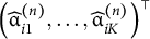 . Because of the computational limitation, the 1,000 MCMC samples were obtained after the first 20,000 iterations for model parameters.
3.2 Results
Table 2 presents 100 times the absolute biases (Abs. Bias) and RMSE, and 95% CI coverage of LCDM parameters (
$\unicode{x3bb}$
 s) of two- or single-level model results. In conditions of small sample sizes and high-quality items, the two-level model provided slightly better absolute biases, RMSE, and 95% CI coverage than the single model. However, under conditions of small sample sizes and low-quality items, the absolute biases, RMSE, and 95% CI coverage of the two-level model were better than those of the single-level model. For example, the 100 times of absolute bias of the two-level in the strong structural parameter condition was 38.82, and that of the single-level was 69.54. In the condition of 100 times, the RMSE of the two-level model was 44.25, and that of the single-level model was 63.43. The value of the 95% CI coverage for the two-level model was 0.971, and that of the single-level model was 0.790, indicating a notable difference. The absolute bias, the RMSE of the two-level model decreased as the sample size increased, and its 95% CI coverages were close to the theoretically preferable value of 0.95. The absolute biases of the single-level model in the 1,000 sample were smaller than those of the 200 sample size, but the values were worse than those of the two-level models. In the same conditions, the RMSE of the single-level model exceeded that of the two-level model. Moreover, the 95% CI coverages of the single-level model were low even in the large sample size conditions. In summary, for the LCDM item parameter recovery, the two-level model exhibited smaller biases and RMSEs and appropriate 95% CI coverage than the single-level model.
One-hundred times the absolute bias (Abs. Bias), root mean square error (RMSE), and 95% credible (95% CI) coverage of log-linear cognitive diagnostic model parameters (
$\unicode{x3bb}$
 s) of two- and single-level model results in Simulation 1
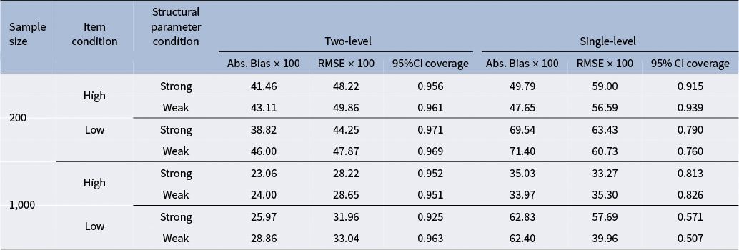
Table 2 Long description
The table presents results for Simulation 1 across eight experimental conditions. The columns are divided into Sample size, Item condition, Structural parameter condition, and two main model categories: Two-level and Single-level. Each model category reports Abs. Bias times 100, R M S E times 100, and 95 percent C I coverage.
* For Sample size 200:
- High Item, Strong Structural: Two-level (41.46, 48.22, 0.956); Single-level (49.79, 59.00, 0.915).
- High Item, Weak Structural: Two-level (43.11, 49.86, 0.961); Single-level (47.65, 56.59, 0.939).
- Low Item, Strong Structural: Two-level (38.82, 44.25, 0.971); Single-level (69.54, 63.43, 0.790).
- Low Item, Weak Structural: Two-level (46.00, 47.87, 0.969); Single-level (71.40, 60.73, 0.760).
* For Sample size 1,000:
- High Item, Strong Structural: Two-level (23.06, 28.22, 0.952); Single-level (35.03, 33.27, 0.813).
- High Item, Weak Structural: Two-level (24.00, 28.65, 0.951); Single-level (33.97, 35.30, 0.826).
- Low Item, Strong Structural: Two-level (25.97, 31.96, 0.925); Single-level (62.83, 57.69, 0.571).
- Low Item, Weak Structural: Two-level (28.86, 33.04, 0.963); Single-level (62.40, 39.96, 0.507).
The attribute mixing proportion parameter
$\boldsymbol{\unicode{x3c0}}$
 exhibited the same tendency. The results are presented in Table 3. The notable difference between the two- and single-level models was 95% CI coverage. The two-level model indicated relatively better values of the 95% CI coverages than the single-level models. The high-quality items or strong structural parameter conditions exhibited better absolute biases than the low-quality or weak structural parameter conditions in the two-level models. In addition, the absolute biases of the two-level model were approximately half of those of the single-level model.
One-hundred times the Abs. Bias, RMSE, and 95% credible (95% CI) coverage of attribute mastery pattern mixing parameters
$\unicode{x3c0}$
 of two- and single-level model results in Simulation 1

Table 3 Long description
The table is structured with nine columns. The first three columns define the conditions: Sample size (200 or 1,000), Item quality condition (High or Low), and Structural parameter condition (Strong or Weak). The remaining six columns are split into two main groups: Two-level and Single-level models. Each group contains three metrics: Abs. Bias times 100, R M S E times 100, and 95 percent C I coverage.
For Sample size 200:
- High quality, Strong: Two-level (1.89, 2.33, 0.958); Single-level (3.24, 3.69, 0.815).
- High quality, Weak: Two-level (2.25, 2.79, 0.935); Single-level (3.69, 3.62, 0.760).
- Low quality, Strong: Two-level (2.47, 3.03, 0.963); Single-level (5.72, 7.07, 0.695).
- Low quality, Weak: Two-level (5.76, 6.13, 0.900); Single-level (6.29, 6.77, 0.605).
For Sample size 1,000:
- High quality, Strong: Two-level (0.96, 1.33, 0.950); Single-level (2.08, 1.78, 0.685).
- High quality, Weak: Two-level (0.92, 1.16, 0.953); Single-level (2.37, 1.67, 0.633).
- Low quality, Strong: Two-level (2.16, 3.16, 0.910); Single-level (5.50, 6.85, 0.633).
- Low quality, Weak: Two-level (2.45, 2.89, 0.918); Single-level (5.14, 3.96, 0.375).
The parameter recovery results for structural parameters on the intercept (
${\unicode{x3b3}}_I^{(P)}$
 of
${\unicode{x3b3}}_I^{(G)}$
of
${\unicode{x3b3}}_I^{(G)}$
 ) are presented in Table 4. The person-level structural parameters
${\unicode{x3b3}}_I^{(P)}$
) are presented in Table 4. The person-level structural parameters
${\unicode{x3b3}}_I^{(P)}$
 of the two-level model exhibited smaller biases and RMSEs than those of the single-level model. For example, in the 1,000 sample, high-quality items, and strong structural parameter conditions, the 100 times of the absolute bias and RMSE of the two-level model were 9.21 and 12.69, and the corresponding values of the single-level model were 73.57 and 62.61, respectively. The 95% CI coverages of the two-level model were generally better than those of the single-level model. The decreases in the biases and RMSE of the two-level model because of sample size increase were affected by item quality. The increase in sample size appropriately decreased the biases and RMSEs in the person-level structural parameters in the high-quality items. However, these decreases were slower in the low-quality item condition. The group-level structural parameter
${\unicode{x3b3}}_I^{(G)}$
of the two-level model exhibited smaller biases and RMSEs than those of the single-level model. For example, in the 1,000 sample, high-quality items, and strong structural parameter conditions, the 100 times of the absolute bias and RMSE of the two-level model were 9.21 and 12.69, and the corresponding values of the single-level model were 73.57 and 62.61, respectively. The 95% CI coverages of the two-level model were generally better than those of the single-level model. The decreases in the biases and RMSE of the two-level model because of sample size increase were affected by item quality. The increase in sample size appropriately decreased the biases and RMSEs in the person-level structural parameters in the high-quality items. However, these decreases were slower in the low-quality item condition. The group-level structural parameter
${\unicode{x3b3}}_I^{(G)}$
 observed only in the two-level model was generally a good recovery; its 95% CI coverage was 1 indicating too large 95% CIs. This was, however, better than those under coverage results because of its conservative tendency. The above tendencies were also observed in the recovery of the structural parameters on the slope (
${\unicode{x3b3}}_S^{(P)}$
observed only in the two-level model was generally a good recovery; its 95% CI coverage was 1 indicating too large 95% CIs. This was, however, better than those under coverage results because of its conservative tendency. The above tendencies were also observed in the recovery of the structural parameters on the slope (
${\unicode{x3b3}}_S^{(P)}$
 of
${\unicode{x3b3}}_S^{(G)}$
of
${\unicode{x3b3}}_S^{(G)}$
 ) presented in Table 5.
One-hundred times the Abs. Bias, RMSE, and 95% credible (95% CI) coverage of structural parameters on intercept (
${\unicode{x3b3}}_I^{(P)}$
 of
${\unicode{x3b3}}_I^{(G)}$
of
${\unicode{x3b3}}_I^{(G)}$
 ) of two- and single-level model results in Simulation 1

Table 4 Long description
The table is structured with three primary header categories: Sample size, Item quality condition, and Structural parameter condition, followed by three performance blocks: Two-level: gamma sub I super (P), Two-level: gamma sub I super (G), and Single-level: gamma sub I super (P). Each performance block contains three metrics: Abs. Bias times 100, R M S E times 100, and 95% C I coverage.
Key data points include:
* For Sample size 200, High quality, Strong condition: Two-level (P) shows Abs. Bias 16.04 and R M S E 19.60; Single-level (P) shows significantly higher Abs. Bias of 62.40.
* For Sample size 200, Low quality, Strong condition: Two-level (P) Abs. Bias is 17.73, while Single-level (P) jumps to 101.51.
* For Sample size 1,000, High quality, Strong condition: Two-level (P) Abs. Bias drops to 9.21, while Single-level (P) remains high at 73.57.
* For Sample size 1,000, Low quality, Strong condition: Two-level (P) Abs. Bias is 19.24, and Single-level (P) reaches its peak bias at 139.79.
* Across all conditions, the Two-level: gamma sub I super (G) model maintains a 95% C I coverage of 1.000.
One-hundred times the Abs. Bias, RMSE, and 95% credible (95% CI) coverage of structural parameters on slope (
${\unicode{x3b3}}_S^{(P)}$
 of
${\unicode{x3b3}}_S^{(G)}$
of
${\unicode{x3b3}}_S^{(G)}$
 ) of two- and single-level model results

Table 5 Long description
The table is structured with three primary columns for conditions: Sample size (200 or 1,000), Item quality condition (High or Low), and Structural parameter condition (Strong or Weak). These are compared against three model performance categories: Two-level: gamma sub S super (P), Two-level: gamma sub S super (G), and Single-level: gamma sub S super (P). Each category reports three metrics: Abs. Bias times 100, R M S E times 100, and 95 percent C I coverage.
Key data points for Sample Size 200:
* High Quality, Strong Condition: Two-level (P) has Abs. Bias 10.06, R M S E 12.53, Coverage 0.966. Single-level (P) has Abs. Bias 28.19, R M S E 32.72, Coverage 0.886.
* Low Quality, Strong Condition: Two-level (P) has Abs. Bias 12.73, R M S E 15.48, Coverage 0.966. Single-level (P) has Abs. Bias 34.52, R M S E 48.64, Coverage 0.949.
Key data points for Sample Size 1,000:
* High Quality, Strong Condition: Two-level (P) has Abs. Bias 4.83, R M S E 6.38, Coverage 0.951. Single-level (P) has Abs. Bias 23.15, R M S E 24.16, Coverage 0.751.
* Low Quality, Strong Condition: Two-level (P) has Abs. Bias 11.41, R M S E 16.20, Coverage 0.923. Single-level (P) has Abs. Bias 45.32, R M S E 54.32, Coverage 0.780.
Across all conditions, the Two-level: gamma sub S super (G) model consistently maintains a 95 percent C I coverage of 1.000.
The results of the variance-related parameters are presented in Tables 6–8. Table 6 presents the values of the covariance matrix parameter of the intercept
$I$
 and slope
$S$
and slope
$S$
 (
${\Sigma}^{(P)}$
(
${\Sigma}^{(P)}$
 or
${\Sigma}^{(G)}$
or
${\Sigma}^{(G)}$
 ). The two-level model exhibited sufficiently small biases and RMSEs of the person-level covariance matrix
${\Sigma}^{(P)}$
). The two-level model exhibited sufficiently small biases and RMSEs of the person-level covariance matrix
${\Sigma}^{(P)}$
 , but the single-level models indicated large values. The 95% CIs of
${\Sigma}^{(P)}$
, but the single-level models indicated large values. The 95% CIs of
${\Sigma}^{(P)}$
 in the two-level models were relatively better than those of the single-level model. However, even in the 1,000 sample size conditions, the values were approximately 0.85 and were not the best. Increase of sample or group sizes might solve this problem. The group-level covariance results
${\Sigma}^{(G)}$
in the two-level models were relatively better than those of the single-level model. However, even in the 1,000 sample size conditions, the values were approximately 0.85 and were not the best. Increase of sample or group sizes might solve this problem. The group-level covariance results
${\Sigma}^{(G)}$
 were generally good, but the 95% CI coverages in the 200 sample size were in the range of 0.820–0.880 and were not the best. Table 7 presents the results of the residual variances (
${\unicode{x3c3}}_{\unicode{x3b5}^{(P)}}^2$
were generally good, but the 95% CI coverages in the 200 sample size were in the range of 0.820–0.880 and were not the best. Table 7 presents the results of the residual variances (
${\unicode{x3c3}}_{\unicode{x3b5}^{(P)}}^2$
 and
${\unicode{x3c3}}_{\unicode{x3b5}^{(G)}}^2$
and
${\unicode{x3c3}}_{\unicode{x3b5}^{(G)}}^2$
 ). Again, the two-level model exhibited better results than the single-level results of the person-level residual variance
${\unicode{x3c3}}_{\unicode{x3b5}^{(P)}}^2$
). Again, the two-level model exhibited better results than the single-level results of the person-level residual variance
${\unicode{x3c3}}_{\unicode{x3b5}^{(P)}}^2$
 . For example, in the 1,000 sample, high-quality items, and strong structural parameter condition, the 100 times of the absolute bias and RMSE of the two-level model were 5.72 and 6.83, and the corresponding values of the single-level model were 13.19 and 11.83, respectively. The group-level residual variance
${\unicode{x3c3}}_{\unicode{x3b5}^{(G)}}^2$
. For example, in the 1,000 sample, high-quality items, and strong structural parameter condition, the 100 times of the absolute bias and RMSE of the two-level model were 5.72 and 6.83, and the corresponding values of the single-level model were 13.19 and 11.83, respectively. The group-level residual variance
${\unicode{x3c3}}_{\unicode{x3b5}^{(G)}}^2$
 of the two-level model was sufficiently small. Finally, Table 8 presents the variance parameter
${\unicode{x3c3}}_{\unicode{x3b8}}^2$
of the two-level model was sufficiently small. Finally, Table 8 presents the variance parameter
${\unicode{x3c3}}_{\unicode{x3b8}}^2$
 of the random effect
${\unicode{x3b8}}_m$
of the random effect
${\unicode{x3b8}}_m$
 . The 200 sample size conditions indicated approximately 120–160 values for the 100 times of the absolute biases and 150–180 for the 100 times of the RMSEs. However, these values for the 1,000 sample size conditions decreased to approximately 54–58 and 65–70, respectively. The results of the 95% CI coverage were appropriate if the sample size was increased. In our simulation, we set
$M=10$
. The 200 sample size conditions indicated approximately 120–160 values for the 100 times of the absolute biases and 150–180 for the 100 times of the RMSEs. However, these values for the 1,000 sample size conditions decreased to approximately 54–58 and 65–70, respectively. The results of the 95% CI coverage were appropriate if the sample size was increased. In our simulation, we set
$M=10$
 for the 100 sample size condition and
$M=25$
for the 100 sample size condition and
$M=25$
 for the 1,000 sample size condition. Therefore, the group number increased as the sample size increased.
One-hundred times the Abs. Bias, RMSE, and 95% credible (95% CI) coverage of covariance matrix parameter of intercept
$\boldsymbol I$
 and slope
$S$
and slope
$S$
 (
${\Sigma}^{(P)}$
(
${\Sigma}^{(P)}$
 or
${\Sigma}^{(G)}$
or
${\Sigma}^{(G)}$
 ) of two- and single-level model results in Simulation 1

Table 6 Long description
The table is organized by Sample size (200 and 1,000), Item quality condition (High and Low), and Structural parameter condition (Strong and Weak).
For Sample size 200:
- High quality, Strong: Two-level Sigma super P has Abs. Bias times 100 of 12.16, R M S E times 100 of 19.62, and 0.927 coverage. Two-level Sigma super G has 1.67, 1.60, and 0.840. Single-level Sigma super P has 569.50, 297.22, and 0.007.
- High quality, Weak: Two-level Sigma super P has 11.52, 22.18, and 0.933. Two-level Sigma super G has 1.73, 1.75, and 0.847. Single-level Sigma super P has 455.37, 209.04, and 0.000.
- Low quality, Strong: Two-level Sigma super P has 11.20, 18.53, and 0.927. Two-level Sigma super G has 1.67, 1.55, and 0.820. Single-level Sigma super P has 458.84, 241.69, and 0.127.
- Low quality, Weak: Two-level Sigma super P has 10.61, 20.95, and 0.927. Two-level Sigma super G has 1.73, 1.72, and 0.880. Single-level Sigma super P has 349.74, 210.67, and 0.000.
For Sample size 1,000:
- High quality, Strong: Two-level Sigma super P has 11.67, 13.18, and 0.853. Two-level Sigma super G has 0.89, 1.30, and 0.947. Single-level Sigma super P has 594.08, 162.17, and 0.000.
- High quality, Weak: Two-level Sigma super P has 11.04, 15.36, and 0.860. Two-level Sigma super G has 0.70, 0.75, and 0.940. Single-level Sigma super P has 431.07, 126.81, and 0.000.
- Low quality, Strong: Two-level Sigma super P has 11.78, 12.91, and 0.847. Two-level Sigma super G has 2.11, 3.11, and 0.867. Single-level Sigma super P has 432.35, 118.18, and 0.153.
- Low quality, Weak: Two-level Sigma super P has 11.40, 15.44, and 0.860. Two-level Sigma super G has 0.75, 0.80, and 0.967. Single-level Sigma super P has 357.00, 133.25, and 0.000.
One-hundred times the Abs. Bias, RMSE, and 95% credible (95% CI) coverage of residual variance of
$T$
 time points outcome measures (
${{\unicode{x3c3}}_{\unicode{x3b5}^{(P)}}^2}$
time points outcome measures (
${{\unicode{x3c3}}_{\unicode{x3b5}^{(P)}}^2}$
 or
${\unicode{x3c3}}_{\unicode{x3b5}^{(G)}}^2$
or
${\unicode{x3c3}}_{\unicode{x3b5}^{(G)}}^2$
 ) of two- and single-level model results in Simulation 1

Table 7 Long description
The table is structured with three primary header categories: Sample size, Item quality condition, and Structural parameter condition, followed by three model outcome groups: Two-level: sigma epsilon super 2 sub P, Two-level: sigma epsilon super 2 sub G, and Single-level: sigma epsilon super 2 sub P. Each outcome group includes three metrics: Abs. Bias times 100, R M S E times 100, and 95 percent C I coverage.
Data for Sample Size 200:
* High Item Quality, Strong Structural: Two-level P (9.71, 12.86, 0.950); Two-level G (3.21, 3.49, 0.920); Single-level P (17.79, 19.29, 0.540).
* High Item Quality, Weak Structural: Two-level P (9.61, 12.62, 0.970); Two-level G (3.08, 3.28, 0.920); Single-level P (17.23, 18.82, 0.545).
* Low Item Quality, Strong Structural: Two-level P (9.41, 12.33, 0.975); Two-level G (3.50, 3.76, 0.925); Single-level P (17.64, 18.78, 0.560).
* Low Item Quality, Weak Structural: Two-level P (9.04, 11.62, 0.975); Two-level G (3.38, 3.38, 0.910); Single-level P (16.86, 17.65, 0.510).
Data for Sample Size 1,000:
* High Item Quality, Strong Structural: Two-level P (5.72, 6.83, 0.980); Two-level G (1.07, 1.26, 0.950); Single-level P (13.19, 11.83, 0.335).
* High Item Quality, Weak Structural: Two-level P (5.69, 7.13, 0.960); Two-level G (1.28, 1.48, 0.930); Single-level P (14.83, 14.08, 0.275).
* Low Item Quality, Strong Structural: Two-level P (9.71, 12.86, 0.950); Two-level G (3.21, 3.49, 0.920); Single-level P (17.79, 19.29, 0.540).
* Low Item Quality, Weak Structural: Two-level P (9.61, 12.62, 0.970); Two-level G (3.08, 3.28, 0.920); Single-level P (17.23, 18.82, 0.545).
One-hundred times the Abs. Bias, RMSE, and 95% credible (95% CI) coverage of the variance
${\unicode{x3c3}}_{\unicode{x3b8}}^2$
 of random effect
${\unicode{x3b8}}_m$
of random effect
${\unicode{x3b8}}_m$
 of two- or single-level model results in Simulation 1

Table 8 Long description
The table presents results for two-level models across eight experimental conditions. The columns are Sample size, Item quality condition, Structural parameter condition, and three metrics under the Two-level heading: Abs. Bias times 100, R M S E times 100, and 95 percent C I coverage.
* For Sample size 200:
- High Item quality and Strong Structural parameter: Abs. Bias 121.40, R M S E 150.85, C I 0.940.
- High Item quality and Weak Structural parameter: Abs. Bias 136.34, R M S E 165.07, C I 0.880.
- Low Item quality and Strong Structural parameter: Abs. Bias 126.72, R M S E 156.54, C I 0.880.
- Low Item quality and Weak Structural parameter: Abs. Bias 158.55, R M S E 183.48, C I 0.880.
* For Sample size 1,000:
- High Item quality and Strong Structural parameter: Abs. Bias 55.35, R M S E 65.33, C I 0.980.
- High Item quality and Weak Structural parameter: Abs. Bias 53.74, R M S E 68.74, C I 0.940.
- Low Item quality and Strong Structural parameter: Abs. Bias 55.90, R M S E 65.45, C I 0.980.
- Low Item quality and Weak Structural parameter: Abs. Bias 57.97, R M S E 70.40, C I 0.940.
Attribute mastery recovery results are shown in Table 9. High-quality items tended to show higher AARs and PARs. Especially, both AARs and PARs exceeded 0.92 for all conditions with the two-level model in the high-quality items conditions. In addition, strong structural models or larger sample sizes indicated higher AARs and PARs than weak or small sample size conditions. For example, AARs of the 200 sample size, low-quality items, and weak structural condition with the two-level model were 0.763–0.784, but those of the 1,000 sample size, low-quality items, and strong structural condition were 0.884–0.894. More importantly, the single-level model provided drastically lower AARs and PARs than the two-level model. This indicated that ignoring multilevel structure resulted in misdiagnosis.
Attribute-level and pattern-level recovery results of two- and single-level models in Simulation 1

Table 9 Long description
The table is organized into columns for Sample size, Item condition, Gamma parameter, and two main model categories: Two-level and Single-level. Each model category includes four metrics: A A R 1, A A R 2, A A R 3, and P A R.
For a Sample size of 200:
* High Item condition, Strong Gamma: Two-level results are A A R 1 0.964, A A R 2 0.963, A A R 3 0.971, P A R 0.929. Single-level results are A A R 1 0.840, A A R 2 0.854, A A R 3 0.867, P A R 0.641.
* High Item condition, Weak Gamma: Two-level results are A A R 1 0.927, A A R 2 0.931, A A R 3 0.934, P A R 0.817. Single-level results are A A R 1 0.822, A A R 2 0.821, A A R 3 0.831, P A R 0.582.
* Low Item condition, Strong Gamma: Two-level results are A A R 1 0.879, A A R 2 0.879, A A R 3 0.899, P A R 0.779. Single-level results are A A R 1 0.677, A A R 2 0.701, A A R 3 0.714, P A R 0.380.
* Low Item condition, Weak Gamma: Two-level results are A A R 1 0.763, A A R 2 0.785, A A R 3 0.784, P A R 0.472. Single-level results are A A R 1 0.668, A A R 2 0.681, A A R 3 0.666, P A R 0.355.
For a Sample size of 1,000:
* High Item condition, Strong Gamma: Two-level results are A A R 1 0.969, A A R 2 0.970, A A R 3 0.976, P A R 0.941. Single-level results are A A R 1 0.843, A A R 2 0.850, A A R 3 0.866, P A R 0.632.
* High Item condition, Weak Gamma: Two-level results are A A R 1 0.944, A A R 2 0.946, A A R 3 0.949, P A R 0.856. Single-level results are A A R 1 0.833, A A R 2 0.834, A A R 3 0.837, P A R 0.607.
* Low Item condition, Strong Gamma: Two-level results are A A R 1 0.884, A A R 2 0.875, A A R 3 0.894, P A R 0.742. Single-level results are A A R 1 0.680, A A R 2 0.698, A A R 3 0.693, P A R 0.363.
* Low Item condition, Weak Gamma: Two-level results are A A R 1 0.821, A A R 2 0.828, A A R 3 0.842, P A R 0.587. Single-level results are A A R 1 0.679, A A R 2 0.681, A A R 3 0.675, P A R 0.371.
Note: A A R is attribute-level agreement ratio and P A R is pattern-level agreement ratio.
Note: AAR is attribute-level agreement ratio and PAR is pattern-level agreement ratio.
Summarily, the two-level model provided smaller absolute biases and RMSEs and a preferable 95% CI coverage than the single-level model for all model parameters in almost all conditions. In other words, multilevel structures should be considered when employing a multistage sampling design. In addition, our estimation method was validated using the JAGS language well recovered model parameters at least in the idealized situations.
4 Simulation study 2
The first simulation employed three attribute Q-matrix which is relatively simple. To generalize the parameter recovery with the Bayesian estimation method employed in the first simulation, we assumed five attribute Q-matrix that represented a complex situation in the second simulation.
4.1 Simulation setting
Table 10 shows the Q-matrix in the second simulation in which the 1st–10th items were simple needing only one attribute to solve them, and the rest 11th–20th items required two attributes representing complex items. The three attributes loading items were not assumed because the number of combinations of two-way interaction is
$\left(\genfrac{}{}{0pt}{}{5}{3}\right)=10$
 ; therefore, the number of item parameters becomes large if we assume items that need three attributes. This is overly complicated, and we did not include these items in the second simulation. In the second simulation, we manipulated the same factors as the first simulation: sample size (200 or 1,000), item quality (high or low), and the structural parameter strength (strong or weak). However, the true parameter values were slightly changed.
Q-matrix for the second simulation study

Table 10 Long description
The table consists of 20 rows representing items and 5 columns representing attributes. Each cell contains either a 1, indicating the presence of an attribute for that item, or a 0, indicating its absence.
* Items 1 and 6 map to Attribute 1.
* Items 2 and 7 map to Attribute 2.
* Items 3 and 8 map to Attribute 3.
* Items 4 and 9 map to Attribute 4.
* Items 5 and 10 map to Attribute 5.
* Item 11 maps to Attributes 1 and 2.
* Item 12 maps to Attributes 1 and 3.
* Item 13 maps to Attributes 1 and 4.
* Item 14 maps to Attributes 1 and 5.
* Item 15 maps to Attributes 2 and 3.
* Item 16 maps to Attributes 2 and 4.
* Item 17 maps to Attributes 2 and 5.
* Item 18 maps to Attributes 3 and 4.
* Item 19 maps to Attributes 3 and 5.
* Item 20 maps to Attributes 4 and 5.
First, in the high-quality items condition, simple items had an intercept
${\unicode{x3bb}}_0=-2$
 and a main effect
${\unicode{x3bb}}_1=4$
and a main effect
${\unicode{x3bb}}_1=4$
 . The complex items had an intercept
${\unicode{x3bb}}_0=-3$
. The complex items had an intercept
${\unicode{x3bb}}_0=-3$
 , two main effects
${\unicode{x3bb}}_1=2$
, two main effects
${\unicode{x3bb}}_1=2$
 , and a first-order interaction
${\unicode{x3bb}}_2=2$
, and a first-order interaction
${\unicode{x3bb}}_2=2$
 . Again, low-quality items had half the parameter values as the high-quality items.
In the strong structural parameter condition, the main effects of the intercept were set to
$\left({\unicode{x3b3}}_{I1}^{(P)},{\unicode{x3b3}}_{I2}^{(P)},{\unicode{x3b3}}_{I3}^{(P)},{\unicode{x3b3}}_{I4}^{(P)},{\unicode{x3b3}}_{I5}^{(P)}\right)=\left(\mathrm{0.6,0.8,1},\mathrm{1.2,1.4}\right)$
 . The second interaction was generated in the same way as the first simulation. The two-way interaction was omitted because of the same reason mentioned above. The weak structural parameter assumed half of the main effects of the intercept in the strong condition. Then the interactions were generated the same way. The other parameter settings and MCMC estimation settings were the same as the first simulation. The evaluation perspectives were also the same as the first simulation. The simulation R codes are shown in the OSF file.
4.2 Results
Even with the five attribute Q-matrix condition, we confirm the similar results shown in the first simulation. The two-level model indicated better estimation results than the single-level models: smaller absolute biases and RMSEs, and more appropriate coverages of 95% CI. Therefore, the evidence of the validity of the estimation with the JAGS language was obtained before conducting real-data analysis with the proposed model in the following section.
Because of the space limitation and to reduce redundancy of the description, the parameter recovery results tables are presented in Tables S1–S6 in the Supplementary Material. We only show attribute mastery recovery results here in Table 11. Most AARs with the two-level in the high-quality items conditions were higher than 0.95, but the ones with the single-level model were at most approximately 0.92. In these conditions, PARs of the two-level model were much better than ones of the single-model. For example, PAR of the two-level model in the condition of the 1,000 sample, high-quality items, and strong structural parameters was 0.931, but corresponding value of the single-level model was 0.638. Differences of AARs or PARs between the two models were evident in low-item conditions. For example, AARs of the two-level in the 200 sample, low-quality items, and strong structural parameter were 0.866–0.895, and those of the single-level model were 0.696–0.725. Furthermore, PAR with the two-level model in the same condition was 0.605, but that with the single-level model was 0.249. In summary, the two-level model relatively better recovered attribute masteries than the single-level model that ignores the multilevel structure.
Attribute-level and pattern-level recovery results of two- and single-level models in Simulation 2

Table 11 Long description
The table is organized by Sample size (200 and 1,000), Item condition (High and Low), and Gamma parameter (Strong and Weak). It compares Two-level and Single-level models using metrics A A R 1 through A A R 5 and P A R.
For Sample size 200:
- High Item Condition, Strong Gamma: Two-level A A R ranges from 0.974 to 0.982, P A R is 0.923. Single-level A A R ranges from 0.881 to 0.916, P A R is 0.645.
- High Item Condition, Weak Gamma: Two-level A A R ranges from 0.949 to 0.967, P A R is 0.828. Single-level A A R ranges from 0.874 to 0.894, P A R is 0.586.
- Low Item Condition, Strong Gamma: Two-level A A R ranges from 0.866 to 0.895, P A R is 0.605. Single-level A A R ranges from 0.696 to 0.728, P A R is 0.249.
- Low Item Condition, Weak Gamma: Two-level A A R ranges from 0.829 to 0.876, P A R is 0.491. Single-level A A R ranges from 0.687 to 0.722, P A R is 0.235.
For Sample size 1,000:
- High Item Condition, Strong Gamma: Two-level A A R ranges from 0.977 to 0.984, P A R is 0.931. Single-level A A R ranges from 0.883 to 0.921, P A R is 0.638.
- High Item Condition, Weak Gamma: Two-level A A R ranges from 0.955 to 0.973, P A R is 0.853. Single-level A A R ranges from 0.873 to 0.898, P A R is 0.592.
- Low Item Condition, Strong Gamma: Two-level A A R ranges from 0.868 to 0.911, P A R is 0.615. Single-level A A R ranges from 0.669 to 0.728, P A R is 0.229.
- Low Item Condition, Weak Gamma: Two-level A A R ranges from 0.843 to 0.895, P A R is 0.550. Single-level A A R ranges from 0.693 to 0.716, P A R is 0.254.
A A R stands for attribute-level agreement ratio and P A R stands for pattern-level agreement ratio.
Note: AAR is attribute-level agreement ratio and PAR is pattern-level agreement ratio.
5 Real-data analysis
In this section, we first describe the following data, item specification, test design, and sampling design and explain the vertical scale construction procedure. The vertical scale was used from the third to the sixth grades in Japanese elementary schools. Next, we explain the attribute definition and Q-matrix construction procedure. These elements were used to define the DCM measurement model at the second-grade level. Additionally, we specify the priors and MCMC settings for the proposed Bayesian data analysis, which are detailed in Section 3.1.3. The parameter estimation results for the linear growth case are presented. We also analyzed a partially freely estimated slope-loading specification as an example of an alternative growth trajectory.
5.1 Data description
5.1.1 Item specification and test design
The difficulty levels of the test items used in this study varied from Grades 2 to 6. All items were produced by Tokyo Shoseki Co., Ltd., Japan, for assessing students’ mathematics ability in Japanese elementary schools. The original item response data are available upon request from the company (https://www.tokyo-shoseki.co.jp/company_english/). Data were also obtained from Mitsunaga and Uesaka (Reference Mitsunaga and Uesaka2025). These items were organized into five test forms and administered across multiple schools from 2018 to 2022. The detailed sampling procedure is described in the next section.
Several items contained two parts: one required students to “write down the formula,” and the other to “calculate the previously answered formula.” However, both parts were treated as a single item, considering their local dependence. The combined items were marked as correct only if the examinee answered both parts correctly. All responses were coded as “correct” and “incorrect,” with no responses coded as missing.
This study used multiple test forms, which included anchor and separate test forms, as presented in Table 12. Each anchor test form comprised two parts: anchor and unique items. Anchor items were administered to focal grade groups (Grades 2–6) and adjacent grades. For example, the anchor test for Grade 3 contained items designated for Grade 3, as well as items for Grades 2 and 4. In this case, Grade 3 items were referred to as unique items, whereas Grades 2 and 4 items were considered anchor items. The separate test forms contained only items at a single difficulty level, corresponding to Grades 2–6, and the items were identical to those in the anchor test forms. The number of test items administered is presented in Table 12.
Number of items in the anchor and separate tests

Table 12 Long description
The table is organized into two main sections: Anchor test and Separate test. The columns include Item difficulty level, No. of items (subdivided by Grade 2, Grade 3, Grade 4, Grade 5, and Grade 6), and a Total column.
Anchor test section:
* Grade 2 difficulty: 19 items for Grade 2, 9 for Grade 3. Total 28.
* Grade 3 difficulty: 9 items for Grade 2, 19 for Grade 3, 10 for Grade 4. Total 38.
* Grade 4 difficulty: 9 items for Grade 3, 19 for Grade 4, 9 for Grade 5. Total 37.
* Grade 5 difficulty: 10 items for Grade 4, 17 for Grade 5, 10 for Grade 6. Total 37.
* Grade 6 difficulty: 8 items for Grade 5, 19 for Grade 6. Total 27.
Separate test section:
* Grade 2 difficulty: 39 items for Grade 2. Total 39.
* Grade 3 difficulty: 37 items for Grade 3. Total 37.
* Grade 4 difficulty: 39 items for Grade 4. Total 39.
* Grade 5 difficulty: 38 items for Grade 5. Total 38.
* Grade 6 difficulty: 38 items for Grade 6. Total 38.
5.1.2 Sampling design
First, we vertically scaled the five tests administered to different grades from 2 to 6. As no anchor items were present in these five tests, termed “original test” forms, we arranged another “anchor tests” forms containing anchor items and administered them to 2,453 students over five grades. Anchor test forms were administered to students in five elementary schools, covering grades 2 through 6. Therefore, 2,453 students completed the anchor tests (Grade 2 = 477, Grade 3 = 504, Grade 5 = 500, and Grade 6 = 488). Eighteen schools were considered for vertical scaling, with an average student number of 64.33 (SD = 22.81, Min = 36, and Max = 114). Separate test forms were administered to students attending schools in a particular city. We collected datasets from five consecutive administrations, spanning from 2018 (Grade 2) to 2022 (Grade 6). These datasets contained dichotomous response data from common examinees over five years. For example, the 2018 and 2019 datasets contained data of Grades 2 and 3 students, respectively. In other words, the longitudinal dataset comprised five dichotomous response datasets administered to the same group of students over five years; no common items were included across separate test forms. GCs were drawn by estimating the mathematics proficiency scores of 1,158 samples from 18 schools (average sample size = 64.333, SD = 23.470, Min = 36, and Max = 114) who took five original test forms for each academic year. These mathematical proficiency scores for these academic years were represented on the vertical scale using the anchor test. Note that the sample that was different from the students who took anchor tests, and this sample was analyzed for the proposed RDC–MGC model.
5.1.3 Vertical scaling procedure
A combined dataset was used to create a scale that can be interpreted as a common ability scale across the five grades. In this study, IRT analysis with a two-parameter logistic (2PL) IRT model was applied to obtain a common scale that could reflect students’ ability levels on the same scale as the item difficulty levels. Before conducting the IRT analysis, we examined local dependencies by comparing Yen’s
${Q}_3$
 statistics (Yen, Reference Yen1984) for each item; no items had values exceeding 0.3. Scree plots were used to assess unidimensionality for each dataset; the largest eigenvalue was significantly higher than the others in every dataset. Therefore, the dataset was considered to generally support the assumptions of unidimensionality and local independence. Although the vertical scaling included second-grade data, the third through sixth grades were used for longitudinal growth analysis. Second-grade data were employed for DCM measurements.
We discuss the measurement invariance of anchor test items between different grades and samples that answered the original and anchor tests. This is because such invariance can be assessed by calculating DIF or using multiple group IRT models. For either point, the unidimensionality of the anchor tests was verified because we constructed a vertical scale using a 2PL IRT model, which requires meeting the assumption of unidimensionality for each subscale of the class. We calculated polychoric correlation matrices and verified whether the largest eigenvalue marked a peak of scree plots for all grades (Table 4 in Mitsunaga & Uesaka, Reference Mitsunaga and Uesaka2025). Based on the result, we concluded that all subscales had sufficient unidimensionality.
Next, the measurement invariance of the anchor test items between different grades was assessed by Lord’s (Reference Lord1980) DIF detection method. We focused on the common items of the adjacent grades (e.g., Grades 3 and 4) test batteries. Then, the item response functions were estimated and assessed DIF between two grades. DIF was detected for almost all cases. However, this was a natural situation for vertical scaling because the different grades had different proficiency levels. The invariance of the anchor test items between the samples that took the original and anchor tests was also verified. Similarly, the DIF between samples was obtained. We analyzed the estimated item response functions of the two groups and found that, unlike discrimination parameters, difficulty parameters were generally similar. The dispersion of the discrimination parameters might be due to differences in the samples. Therefore, only the invariance of item difficulty was acceptable.
In this study, we used the concurrent calibration method to construct the vertical scale, as this method effectively aligned students’ abilities with item difficulty levels across grades (Mitsunaga & Uesaka, Reference Mitsunaga and Uesaka2025). The comparison between separate and concurrent calibrations, two major vertical scaling methods in IRT, was discussed in Lee and Lee (Reference Lee, Lee, Irwing, Booth and Hughes2018) and Hanson and Béguin (Reference Hanson and Béguin2002). Mathematical abilities were estimated using the expected a posteriori (EAP) method, which was used in the GC model. The vertical scaling procedure was performed using the default settings of the “tam.mml.2pl” function in the TAM package (Robitzsch et al., Reference Robitzsch, Kiefer and Wu2022), adopting a multiple group design with the reference group set as Grade 4 students. Mathematical ability was assumed to follow a standard normal distribution.
5.2 Attribute definitions and Q-matrix construction procedure
To define the attributes and Q-matrix for the second-grade test items, we briefly review the background cognitive theory of mathematical tests. Deep understanding involves grasping the interrelations among various types of knowledge, whereas shallow understanding pertains to rote memorization and superficial application of procedures in problem-solving (e.g., Koedinger et al., Reference Koedinger, Corbett and Perfetti2012; Saso et al., Reference Saso, Oka, Uesaka and Usami2024). Deep understanding is more conducive to reinforcing long-term memory and flexibly transferring knowledge to other contexts than shallow understanding (e.g., Koedinger et al., Reference Koedinger, Corbett and Perfetti2012). An example of a deep understanding of mathematical procedures is comprehending the principles behind the construction of the procedures or understanding why they are useful. Similarly, a deep understanding of mathematical terms entails knowing their meanings and providing concrete examples. Lachner and Nückles (Reference Lachner and Nückles2016) discussed the former, and Rittle-Johnson and Alibali (Reference Rittle-Johnson and Alibali1999) the latter.
Saso et al. (Reference Saso, Oka, Uesaka and Arai2023a, Reference Saso, Oka and Uesaka2023b, Reference Saso, Oka, Uesaka and Usami2024) employed DCMs to diagnose attributes, such as shallow and deep understanding of mathematical terms, shallow and deep understanding of mathematical procedures/formulas, and calculation skills. In this study, following Saso et al. (Reference Saso, Oka, Uesaka and Arai2023a, Reference Saso, Oka and Uesaka2023b, Reference Saso, Oka, Uesaka and Usami2024), the third author defined the attributes and constructed an initial Q-matrix. The third author, specializing in educational psychology, holds teaching licenses for elementary school and mathematics at the middle and high school levels in Japan. These attributes were based on the contents of the second-grade level tests. As a result, the following attributes were defined: “A1. Shallow understanding of mathematical procedures,” “A2. Deep understanding of mathematical procedures,” and “A3. Calculation skills.” Note that attributes related to the understanding of mathematical terms were not included in the current study, as the test items did not assess them.
The definitions are as follows: First, the A1 attribute was defined as “understanding how to construct equations from problem statements, reading the hands of a clock, or comparing lengths.” Second, the A2 attribute was defined as “understanding the meaning of procedures and connecting them to concrete examples or diagrammatic representations.” Third, the A3 attribute was defined as “the ability to correctly perform addition, subtraction, multiplication, and division between integers.”
To clarify these attributes, we provided examples of test items. For example, the A1 attribute was measured by Q23, Q24, and Q29. The problem statements for Q23 and Q24 were as follows: “There are 9 apples. There are 3 more oranges than apples. How many oranges are there?” These items required constructing equations to calculate the total number of oranges. Additionally, Q29 asked, “Read the clock when Hiroki got to the park,” and included an illustration of a clock. This item required reading the hands of the clock. Q27, which also measured A1, asked, “Compare the lengths. Which one is the longest?” This item assessed the ability to compare lengths.
Examples measuring the A2 attribute included Q33 and Q16. Q33 asked, “Which story matches the math sentence
$7-4$
 ? Choose one and mark the number with an O,” requiring the understanding of the equation “7 – 4” and its connection to an actual context. Q16 shown in Figure 2 asked, “Satoko is thinking about how to calculate
$7+4$
? Choose one and mark the number with an O,” requiring the understanding of the equation “7 – 4” and its connection to an actual context. Q16 shown in Figure 2 asked, “Satoko is thinking about how to calculate
$7+4$
 . Fill in the blank with the correct number,” which required understanding the meaning of the equation “
$7+4$
. Fill in the blank with the correct number,” which required understanding the meaning of the equation “
$7+4$
 ” and the procedure for calculation with regrouping. Figure 2 illustrates questions related to understanding the principle of calculation. To answer the item, students need to understand the principle of carry-up calculation; they must divide 4 into 3 and 1 against 7 to make 10: (7 + 3) + 1. A2 attribute (deep understanding of mathematical procedures) requires students to understand and solve problems connecting the principle and daily life situations or charts representing the making-ten strategy. Therefore, this calculation process is not only a simple calculation assumed as the A3 attribute (calculation skills). Finally, Q1 (“5+2”) and Q7 (“13-9”) measured the A3 attribute by requiring integer calculations.
Modified question of Q16.

After the third author constructed the initial Q-matrix, the fourth author, an educational psychologist, and third author discussed and confirmed the structure of the initial Q-matrix from the perspective of the content of the test items and theories of the depth of understanding. Specifically, the third author first explained the definitions of the attributes to the fourth author, and they discussed any discrepancies between the item contents and attribute definitions for each item. As the attributes reflected the nature of the items, they concluded that the items appropriately measured the attributes. The revised Q-matrix was obtained as the final version. Table 13 presents the Q-matrix for the RDCM and the descriptive statistics for each item in the second-grade test form.
Q-matrix, mean, and standard deviation (SD) of dichotomous item responses for each item

Table 13 Long description
The table consists of six columns: Item, Attribute A 1 (Shallow understanding of mathematical procedures), Attribute A 2 (Deep understanding of mathematical procedures), Attribute A 3 (Calculation skills), Mean, and S D.
* Items Q 1 through Q 10 map exclusively to A 3 (values: 0, 0, 1) with means ranging from 0.932 to 0.990.
* Items Q 11 through Q 15, Q 17.Q 18, Q 19.Q 20, Q 21.Q 22, Q 23.Q 24, Q 25, Q 26, and Q 39 map to both A 1 and A 3 (values: 1, 0, 1).
* Item Q 16 and Q 37 map to all three attributes A 1, A 2, and A 3 (values: 1, 1, 1). Q 16 has the lowest mean in this group at 0.636.
* Items Q 27 through Q 31, Q 34, and Q 35 map exclusively to A 1 (values: 1, 0, 0).
* Items Q 32, Q 33, Q 36, and Q 38 map to A 1 and A 2 (values: 1, 1, 0). Q 38 shows the lowest overall mean in the table at 0.392 and the highest S D at 0.488.
Binary values (1 for presence, 0 for absence) define the attribute requirements for each item.
Note that shallow and deep understanding could theoretically form a linear attribute hierarchy (Leighton et al., Reference Leighton, Gierl and Hunka2004); the Q-matrix reflected this structure. However, this hierarchy was partial, as A3 was not included in the linear structure. The attribute hierarchy is more appropriate for a large number of attributes, as it reduces the number of parameters. This study utilized only three attributes, assuming a structure would result in information loss during parameter estimation. Therefore, no structure was assumed for parameter estimation. Under the final Q-matrix setting, the generic identifiability of the DCM parameter estimation (Chen et al., Reference Chen, Culpepper and Liang2020) was satisfied. The detailed estimation settings will be presented in the next section.
5.3 Data analysis settings
The entire sample size was 1,158. The 35 items from the second grade were used for diagnostic assessment. The mathematics abilities, based on vertically scaled tests from the third to sixth grades, were used for the growth model. These grades will be referred to as the first to fourth time points hereafter. Furthermore, data were collected from 18 schools and used to estimate group-level parameters and random intercepts in the DCM model.
We assumed three types of DCMs for the second grade: the LCDM, C-RUM, and DINA models. The LCDM is a saturated DCM that assumes all possible interaction terms among attributes. The DINA model is the simplest DCM, containing only slip and guessing parameters for each item. In the LCDM notation, the DINA model assumes only the intercept and highest interaction term, which can be considered a reparametrized version of the DINA model (e.g., DeCarlo, Reference DeCarlo2011). The C-RUM is intermediate between the LCDM and DINA models, as it includes only intercept and main effects. For each of these DCMs, we assumed single- and two-level models. In the single-level model, the random intercept, the group-level growth model, and the corresponding structural model were not assumed. The combination of DCMs and model levels results in six possible models: two-level LCDM, single-level LCDM, two-level C-RUM, single-level C-RUM, two-level DINA, and single-level DINA models. These six models were compared first based on the widely applicable information criterion (WAIC; Watanabe, Reference Watanabe2010). Then, we interpreted the estimated parameters of the best model based on the WAIC.
Prior settings were as follows: The priors for the DCM parameters followed the approach by Zhan, Jiao, Man, et al. (Reference Zhan, Jiao, Man and Wang2019). All priors were modeled with normal distributions, and their variance parameters were fixed at 4. The means of the prior distributions differed among effects: the intercept had a mean of
$-1.096$
 , whereas the main and interaction effects had means of 0, with the main effects positively constrained. The parameters for the Dirichlet distribution for the attribute pattern mixing parameter were set to
$\boldsymbol{\unicode{x3b4}} ={\textbf{1}}_L.$
, whereas the main and interaction effects had means of 0, with the main effects positively constrained. The parameters for the Dirichlet distribution for the attribute pattern mixing parameter were set to
$\boldsymbol{\unicode{x3b4}} ={\textbf{1}}_L.$
 An inverse gamma distribution with
$a=0.01$
An inverse gamma distribution with
$a=0.01$
 and
$b=0.01$
and
$b=0.01$
 was used for the variance
${\unicode{x3c3}}_{\unicode{x3b8}}^2$
was used for the variance
${\unicode{x3c3}}_{\unicode{x3b8}}^2$
 of the random effect. The priors for the MGC components were mainly related to variance parameters. The parameters for the inverse gamma distributions for
${\unicode{x3c3}}_{\epsilon_t^{(G)}}^2$
of the random effect. The priors for the MGC components were mainly related to variance parameters. The parameters for the inverse gamma distributions for
${\unicode{x3c3}}_{\epsilon_t^{(G)}}^2$
 and
${\unicode{x3c3}}_{\epsilon_{tm}^{(P)}}^2$
and
${\unicode{x3c3}}_{\epsilon_{tm}^{(P)}}^2$
 were set to
$a=0.01$
were set to
$a=0.01$
 and
$b=0.001$
and
$b=0.001$
 , respectively. An inverse Wishart distribution was used for
${\Sigma}^{(P)}$
, respectively. An inverse Wishart distribution was used for
${\Sigma}^{(P)}$
 and
${\Sigma}^{(G)}$
and
${\Sigma}^{(G)}$
 with a two-dimensional identity matrix
$\Psi$
with a two-dimensional identity matrix
$\Psi$
 and 10 degrees of freedom
$\unicode{x3bd}$
and 10 degrees of freedom
$\unicode{x3bd}$
 . The structural model parameters were controlled by normal distributions. The attribute effects on the intercept,
${\unicode{x3b3}}_I^{(P)}$
. The structural model parameters were controlled by normal distributions. The attribute effects on the intercept,
${\unicode{x3b3}}_I^{(P)}$
 s, had a normal distribution with a mean of 0.5 and variance of 1.0, as we assumed that attribute mastery could affect the mathematics ability of the following year. The priors for the attribute effects on the slope
${\unicode{x3b3}}_S^{(P)}$
s, had a normal distribution with a mean of 0.5 and variance of 1.0, as we assumed that attribute mastery could affect the mathematics ability of the following year. The priors for the attribute effects on the slope
${\unicode{x3b3}}_S^{(P)}$
 and group-level effects
${\unicode{x3b3}}_I^{(G)}$
and group-level effects
${\unicode{x3b3}}_I^{(G)}$
 and
${\unicode{x3b3}}_S^{(G)}$
and
${\unicode{x3b3}}_S^{(G)}$
 were modeled with standard normal distributions.
We employed Bayesian estimation based on the JAGS language (Plummer, Reference Plummer2003). Preliminary MCMC iterations revealed that some structural parameters were not identified, necessitating their fixation. Specifically, the attribute mastery pattern (110) was not estimated in the two-level LCDM; therefore,
${\unicode{x3b3}}_{I12}^{(P)}$
 and
${\unicode{x3b3}}_{S12}^{(P)}$
and
${\unicode{x3b3}}_{S12}^{(P)}$
 were fixed at 0. Additionally,
${\unicode{x3b3}}_{I13}^{(P)}$
were fixed at 0. Additionally,
${\unicode{x3b3}}_{I13}^{(P)}$
 and
${\unicode{x3b3}}_{S13}^{(P)}$
and
${\unicode{x3b3}}_{S13}^{(P)}$
 , which were in the single-level LCDM, were fixed at 0 owing to the inverse association observed in the MCMC trace plots for
${\unicode{x3b3}}_{I1}^{(P)}$
, which were in the single-level LCDM, were fixed at 0 owing to the inverse association observed in the MCMC trace plots for
${\unicode{x3b3}}_{I1}^{(P)}$
 and
${\unicode{x3b3}}_{I13}^{(P)}$
and
${\unicode{x3b3}}_{I13}^{(P)}$
 , as well as for
${\unicode{x3b3}}_{S1}^{(P)}$
, as well as for
${\unicode{x3b3}}_{S1}^{(P)}$
 and
${\unicode{x3b3}}_{S13}^{(P)}$
and
${\unicode{x3b3}}_{S13}^{(P)}$
 . The two- and single-level C-RUM models applied the same constraints as the LCDMs.
In the two- and single-level DINA models, the structural parameters were not well identified; hence, we only assumed the highest interaction parameters,
${\gamma}_{I123}^{(P)}$
 and
${\gamma}_{S123}^{(P)}$
and
${\gamma}_{S123}^{(P)}$
 , consistent with their measurement models. The conditions of general identifiability proposed in Chen et al. (Reference Chen, Culpepper and Liang2020, p. 128) can be explained as follows: the Q-matrix should measure each attribute, and each attribute should be measured by more than two items. This implies that the Q-matrix in our real-data analysis satisfies generic identifiability. Therefore, the general LCDM measurement model is identifiable. However, a reviewer pointed out that the completeness condition defined in Chiu et al. (Reference Chiu, Douglas and Li2009, p. 643) was not satisfied. In our current data analysis setting, we constrained
$\gamma$
, consistent with their measurement models. The conditions of general identifiability proposed in Chen et al. (Reference Chen, Culpepper and Liang2020, p. 128) can be explained as follows: the Q-matrix should measure each attribute, and each attribute should be measured by more than two items. This implies that the Q-matrix in our real-data analysis satisfies generic identifiability. Therefore, the general LCDM measurement model is identifiable. However, a reviewer pointed out that the completeness condition defined in Chiu et al. (Reference Chiu, Douglas and Li2009, p. 643) was not satisfied. In our current data analysis setting, we constrained
$\gamma$
 parameters that are the path coefficients of attribute mastery to latent growth intercepts or slope in the DINA model case. However, that was enough based on the comment. We included additional constraints to restrict the attribute mastery pattern and eliminate indistinguishable attribute mastery patterns. Especially, the (010) pattern, which means mastering only a deep understanding of mathematics, could not be estimated with the Q-matrix. Therefore, the pattern was eliminated from the DINA model. Then, we estimated the model parameters.
Furthermore, a reviewer pointed out that a deep understanding of mathematical procedure might not be measured appropriately. Therefore, we conducted the same analysis for the collapsed Q-matrix that has the combined attribute “the understanding of mathematical procedure” which might be more appropriate than the original deep understanding attribute. Because MCMC iterations, except for the two-level LCDM with the collapsed Q-matrix, did not converge well and the model indicated a WAIC value worse than that of the best model with the original Q-matrix, which will be shown subsequently, the results are provided in Supplementary Material B. This indicated that the merged attribute setting was not appropriate for this dataset, and the shallow and deep understandings of mathematical procedures should have been distinguished.
In addition to the above model and the additional comment of the same reviewer, we conducted the same analysis assuming attribute hierarchy between shallow and deep understanding attributes of the original Q-matrix under the two-level LCDM that was the best fit model shown later. This analysis was intended to include intuitive relationship between the two attributes. Note that attribute hierarchy and measurement appropriateness refer to different points. The hierarchy assumption is about the relationship between attributes, and the measurement appropriateness is about between the attribute and items. Therefore, we believe that assuming attribute hierarchy does not solve the problem associated with the deep understanding attribute discussed above. Even under this consideration, for the reader interested in this hierarchy perspective, we conducted the additional analysis including the attribute hierarchy structure. However, MCMC iterations of four parameters did not converge. The WAIC value was 29,431.201(SE = 258.923) and larger than that from the best fitted model shown in Section 5.4. Therefore, it was concluded that the attribute hierarchy assumption was not appropriate in this data set.
Based on the parameter settings and computational memory limitations, different MCMC sampling settings were assumed. For the two-level LCDM, we employed two chains, each with a length of 80,000 iterations. The first three-fourths of the chain length served as the burn-in period; the thinning interval was set to 20. For the single-level LCDM, we used three chains, each with a length of 60,000 iterations. The burn-in period comprised the first half, and the thinning interval was 10. The MCMC settings for the two- and single-level C-RUM and DINA models were similar to those for the single-level LCDM, with the exception of a chain length of 40,000 iterations. These settings resulted in converged MCMC iterations for the model parameters (
$\widehat{R}<1.1$
 ). After convergence, the attribute mastery patterns and log-likelihood for WAIC were sampled. For the LDCMs, 30,000 iterations were used for three chains with a thinning interval of 10, whereas for the other models, 20,000 iterations were used.
The MCMC iterations were conducted using the “jagsUI” package (Kellner, Reference Kellner2024), and the “psych” package (Revelle, Reference Revelle2024) was used to calculate descriptive statistics. Parameter estimates were interpreted using posterior means and 95% CI. Attribute mastery patterns were calculated based on posterior attribute mastery probabilities. If the posterior probability of attribute mastery exceeded 0.5, the attribute was considered mastered; otherwise, it was considered non-mastered. The main data analysis code is available on the Open Science Framework website: https://osf.io/gpztw.
5.4 Results
We first examined the descriptive statistics for the second-grade diagnostic test and the mathematics ability growth from the third to sixth grade. Table 14 presents the means (correct response ratios) and standard deviations (SDs) for each item. The test items generally showed a correct response ratio exceeding 0.7, indicating that the test was relatively easy. Item Q38 was the most difficult, with a difficulty index of 0.392.
Descriptive statistics of mathematics ability for each grade

Table 14 Long description
The table contains nine columns: Grade, Mean, S E in parentheses, S D, Median, Minimum, Max, Skewness, and Kurtosis.
* Grade 3: Mean minus 0.856, S E 0.022, S D 0.749, Median minus 0.802, Minimum minus 3.685, Max 0.521, Skewness minus 0.529, Kurtosis 0.209.
* Grade 4: Mean 0.135, S E 0.026, S D 0.887, Median 0.183, Minimum minus 3.893, Max 1.742, Skewness minus 0.398, Kurtosis 0.058.
* Grade 5: Mean 1.141, S E 0.029, S D 0.997, Median 1.187, Minimum minus 2.579, Max 2.812, Skewness minus 0.383, Kurtosis minus 0.150.
* Grade 6: Mean 2.505, S E 0.030, S D 1.032, Median 2.539, Minimum minus 1.845, Max 4.452, Skewness minus 0.224, Kurtosis minus 0.372.
Table 14 presents descriptive statistics for mathematics abilities from the third to sixth grade. As expected, the ability gradually increased over time. The minimum and maximum values suggested some overlap between grades. For instance, even in the sixth grade, some students scored lower than the average of third-grade students, and some third-grade students outperformed the average fourth-grade student. This implies that certain students may be significantly behind their actual chronological grade in mathematics ability. Therefore, early diagnosis for intervention is necessary, and the lack of specific cognitive attributes should be assessed.
Table 12 presents the WAIC values for the six models. The two-level LCDM showed the smallest WAIC value (WAIC = 29,329.382, SE = 259.045), followed by the two-level C-RUM (WAIC = 29,367.400, SE = 258.766). Generally, the two-level models demonstrated better WAIC values, indicating the necessity of a multilevel structure. Data also indicated that simpler diagnostic measurement models were not appropriate for this case. Therefore, we interpreted the estimated parameters based on the two-level LCDM. After fitting the aforementioned models, we constrained the structural parameters of the two-level LCDM with 95% CI and included zero to refit the model in a stepwise manner. More precisely, we assumed three models that constrained the zero two-way interaction, the zero two-way and one-way interactions, and the main and interaction effects. These stepwise constraint models can help to inform which levels of the structural parameters are important. The WAICs of the constrained two-way interactions model, constrained one- and two-way interaction model, and constrained main and interactions model were 29,324.504 (SE = 258.994), 29,366.092 (SE = 259.102), and 29,362.482 (SE = 259.063), respectively. The constrained two-way interactions model indicated slightly better WAIC than the freely estimated two-level LCDM presented in Table 15, but the difference was small against SEs. This difference might be ignorable, but it might be possible that two-way interaction was not more important than the other one-way interactions or main effects whose 95% CIs covered 0. In addition to WAIC values, this was the first application example of the proposed method; it is informative to include parameter estimation results as much as possible. Therefore, we focused on the original two-level LCDM hereafter.
WAIC values for the estimated models

Table 15 Long description
The table consists of five columns. The first column lists the Measurement model. The next two columns fall under the Two-level category, providing W A I C and S E values. The final two columns fall under the Single-level category, also providing W A I C and S E values.
* Row 1: L C D M. Two-level W A I C is 29,329.382 (bolded) with an S E of 259.045. Single-level W A I C is 29,847.227 with an S E of 260.411.
* Row 2: C-R U M. Two-level W A I C is 29,367.400 with an S E of 258.766. Single-level W A I C is 29,866.522 with an S E of 259.709.
* Row 3: D I N A. Two-level W A I C is 31,638.806 with an S E of 266.450. Single-level W A I C is 32,469.658 with an S E of 265.039.
Note: L C D M is log-linear cognitive diagnostic mode, C-R U M is compensatory reduced unified model, and D I N A is deterministic input noisy A N D-gate model.
Note: LCDM is log-linear cognitive diagnostic model, C-RUM is compensatory reduced unified model, and DINA is deterministic input noisy AND-gate model.
Table 16 presents the LCDM parameter estimates. Because of space limitations, Table 16 only presents posterior means. However, the complete table, including 95% CI (Table S11 in the Supplementary Material) , is available on the OSF web page. Notably, all 95% CIs for the interaction parameters included zero. If we set these interactions to zero, the LCDM would reduce to the C-RUM. However, the interactions for Q14,
${\unicode{x3bb}}_{13}=1.064\;\left(95\% \mathrm{CI}\left[-0.622,3.267\right]\right)$
 and Q36,
${\unicode{x3bb}}_{12}=0.610\;\left(95\%\mathrm{CI}\left[-0.146,1.349\right]\right)$
and Q36,
${\unicode{x3bb}}_{12}=0.610\;\left(95\%\mathrm{CI}\left[-0.146,1.349\right]\right)$
 had lower bounds close to zero, indicating that these interactions were relatively far from the null value. By contrast, other interactions, such as
${\unicode{x3bb}}_{12}$
had lower bounds close to zero, indicating that these interactions were relatively far from the null value. By contrast, other interactions, such as
${\unicode{x3bb}}_{12}$
 for Q16, showed
${\unicode{x3bb}}_{12}=1.064\; (95\%\mathrm{CI}\left[-2.537,3.576\right]$
for Q16, showed
${\unicode{x3bb}}_{12}=1.064\; (95\%\mathrm{CI}\left[-2.537,3.576\right]$
 ), indicating that this interaction could be considered negligible.
Parameter estimate of LCDM parameters

Table 16 Long description
The table consists of 9 columns: Item, lambda sub 0, lambda sub 1, lambda sub 2, lambda sub 3, lambda sub 12, lambda sub 13, lambda sub 23, and lambda sub 123.
Key data points include:
* Q1: lambda sub 0 is 3.119, lambda sub 3 is 0.706.
* Q11: lambda sub 0 is 0.156, lambda sub 1 is 3.370, lambda sub 3 is 3.723, lambda sub 13 is minus 1.841.
* Q16: lambda sub 0 is minus 3.308, lambda sub 1 is 1.915, lambda sub 2 is 1.551, lambda sub 3 is 0.987, lambda sub 12 is 0.421, lambda sub 13 is minus 0.791, lambda sub 23 is 0.596, lambda sub 123 is 0.815.
* Q23.Q24: lambda sub 0 is minus 1.094, lambda sub 1 is 0.230, lambda sub 3 is 0.264, lambda sub 13 is 1.482.
* Q37: lambda sub 0 is minus 2.396, lambda sub 1 is 2.297, lambda sub 2 is 1.137, lambda sub 3 is 1.073, lambda sub 12 is minus 0.333, lambda sub 13 is minus 1.055, lambda sub 23 is 0.461, lambda sub 123 is minus 0.459.
* Q39: lambda sub 0 is minus 0.456, lambda sub 1 is 1.801, lambda sub 3 is 1.500, lambda sub 13 is minus 0.454.
Most items (Q1 to Q10) only have values for lambda sub 0 and lambda sub 3. Items Q11 to Q15 add lambda sub 1 and lambda sub 13. Complex interactions involving lambda sub 12, lambda sub 23, and lambda sub 123 appear primarily in Q16 and Q37.
Table 17 presents the parameter estimates for the mixing parameters of attribute mastery patterns. The pattern (110) was nearly zero:
$0.003\;\left(95\%\mathrm{CI}\left[0.000,.014\right]\right)$
 , as observed in the preliminary analysis. The patterns (111), (101), and (011) exhibited relatively larger values:
${\unicode{x3c0}}_{111}=0.396\;\left(95\%\mathrm{CI}\left[0.312,.472\right]\right),{\unicode{x3c0}}_{101}=0.211\;\left(95\%\mathrm{CI}\left[\mathrm{0.129,0.296}\right]\right),$
, as observed in the preliminary analysis. The patterns (111), (101), and (011) exhibited relatively larger values:
${\unicode{x3c0}}_{111}=0.396\;\left(95\%\mathrm{CI}\left[0.312,.472\right]\right),{\unicode{x3c0}}_{101}=0.211\;\left(95\%\mathrm{CI}\left[\mathrm{0.129,0.296}\right]\right),$
 and
${\unicode{x3c0}}_{011}=0.144\;(95\%\mathrm{CI}[0.094, 0.193])$
and
${\unicode{x3c0}}_{011}=0.144\;(95\%\mathrm{CI}[0.094, 0.193])$
 . Given that the second-grade diagnostic test was easy, the mixing probabilities reflected the ease of the test. However, although the mixing probability for only one attribute mastery pattern was less than 0.10, the estimates indicate that such a pattern may still exist in the population.
Estimates of the attribute pattern mixing parameters

Table 17 Long description
The table consists of three columns: Attribute mastery pattern, Mean, and 95 percent C I (Lower, Upper).
* Pattern 000: Mean 0.077, C I (0.053, 0.101).
* Pattern 100: Mean 0.085, C I (0.043, 0.136).
* Pattern 010: Mean 0.019, C I (0.006, 0.039).
* Pattern 110: Mean 0.003, C I (0.000, 0.014).
* Pattern 001: Mean 0.065, C I (0.032, 0.104).
* Pattern 101: Mean 0.211, C I (0.129, 0.296).
* Pattern 011: Mean 0.144, C I (0.094, 0.193).
* Pattern 111: Mean 0.396, C I (0.312, 0.472).
Table 18 presents the parameter estimates for the structural model components. The person-level main effects on the intercept were positive, and their 95% CIs did not include zero:
${\unicode{x3b3}}_{I1}^{(P)}=0.852 \left(95\%\mathrm{CI}\left[0.606,1.062\right]\right)$
 ,
${\unicode{x3b3}}_{I2}^{(P)}=0.913\;\left(95\%\mathrm{CI}\left[0.439,1.280\right]\right)$
,
${\unicode{x3b3}}_{I2}^{(P)}=0.913\;\left(95\%\mathrm{CI}\left[0.439,1.280\right]\right)$
 , and
${{\unicode{x3b3}}_{I3}^{(P)}=0.358(95\%\mathrm{CI}[0.107, 0.627])}$
, and
${{\unicode{x3b3}}_{I3}^{(P)}=0.358(95\%\mathrm{CI}[0.107, 0.627])}$
 . This indicates that a shallow and deep understanding of mathematical procedures, as well as calculation skills, predict mathematical ability in the third grade. Interestingly, a deep understanding of mathematical procedures negatively affected the slope (
${\unicode{x3b3}}_{S2}^{(P)}=-0.237,95\%\mathrm{CI}\left[-0.425,-0.016\right]$
. This indicates that a shallow and deep understanding of mathematical procedures, as well as calculation skills, predict mathematical ability in the third grade. Interestingly, a deep understanding of mathematical procedures negatively affected the slope (
${\unicode{x3b3}}_{S2}^{(P)}=-0.237,95\%\mathrm{CI}\left[-0.425,-0.016\right]$
 ). Furthermore, the interaction between a deep understanding of mathematical procedures and calculation skills positively affected the slope
$\left({\unicode{x3b3}}_{S23}^{(P)}=0.284,95\%\mathrm{CI}\left[0.048,0.499\right]\right)$
). Furthermore, the interaction between a deep understanding of mathematical procedures and calculation skills positively affected the slope
$\left({\unicode{x3b3}}_{S23}^{(P)}=0.284,95\%\mathrm{CI}\left[0.048,0.499\right]\right)$
 . These effects are discussed subsequently.
Parameter estimates of the structural model part

Table 18 Long description
The table is divided into two main levels: Person level and Group level.
At the Person level, six parameters are listed:
1. Main effect of attribute 1 (gamma sub 1 super P): Intercept mean 0.852 (C I 0.606 to 1.062); Slope mean minus 0.023 (C I minus 0.120 to 0.076).
2. Main effect of attribute 2 (gamma sub 2 super P): Intercept mean 0.913 (C I 0.439 to 1.280); Slope mean minus 0.237 (C I minus 0.425 to minus 0.016).
3. Main effect of attribute 3 (gamma sub 3 super P): Intercept mean 0.358 (C I 0.107 to 0.627); Slope mean 0.016 (C I minus 0.099 to 0.126).
4. Interaction effect of attributes 1 and 3 (gamma sub 13 super P): Intercept mean 0.147 (C I minus 0.162 to 0.458); Slope mean 0.071 (C I minus 0.078 to 0.214).
5. Interaction effect of attributes 2 and 3 (gamma sub 23 super P): Intercept mean minus 0.253 (C I minus 0.720 to 0.226); Slope mean 0.284 (C I 0.048 to 0.499).
6. Interaction effect of attributes 1 to 3 (gamma sub 123 super P): Intercept mean minus 0.247 (C I minus 0.493 to 0.044); Slope mean 0.030 (C I minus 0.095 to 0.149).
At the Group level, one parameter is listed:
1. Effect of random intercept (gamma super G): Intercept mean minus 2.107 (C I minus 3.261 to minus 1.220); Slope mean 0.936 (C I 0.397 to 1.682).
Bolded values indicate statistical significance where the confidence interval does not cross zero.
Figure 3 illustrates the descriptive growth lines of mathematics ability by attribute mastery patterns. The effects of attribute mastery are evident in the figure. For example, the growth lines of individuals with the (000) attribute mastery pattern (upper-left panel) were generally lower than those of individuals with the (111) pattern (bottom-left panel). In the second upper panels, the slope of the (010) pattern appears slightly flatter than that of the (001) pattern. The estimated effects of attribute mastery on the growth lines were also supported by visual inspection. Notably, some students exhibited atypical growth trajectories. For example, the bottom line of the (001) pattern from third to fifth grade exhibited lower values but caught up in the sixth grade. The line for the (000) pattern, in contrast, did not show improvement throughout the period. These diagnostic test results may highlight severe cases for educational administrators and teachers, and it is crucial to closely monitor such cases. Figure 4 shows the GC of the difference in academic ability for each attribute mastery. As seen later, the mastery of each attribute indicated a higher level of academic proficiency at the third grade, intercepted in the proposed model. In these plots, the slopes of the GCs for mastery and non-mastery of attributes were similar. However, mastery of attributes affected the slope parameters, as discussed subsequently.
Growth patterns of academic ability for each attribute mastery status.

Figure 3 Long description
The figure consists of eight line graphs arranged in a two-column by four-row grid. Each graph shares the same axes: the x-axis represents Grade from 3 to 6, and the y-axis represents Academic Ability from negative 4.5 to 4.5. Individual student trajectories are shown as semi-transparent grey lines.
* Top-left: Attribute Pattern 000 shows a moderate density of lines starting between negative 3 and negative 1.5, with a steady upward linear increase.
* Top-right: Attribute Pattern 100 shows a similar upward trend but with a slightly higher starting point and greater density.
* Second row left: Attribute Pattern 010 contains fewer lines, showing a sparse but consistent upward trend.
* Second row right: Attribute Pattern 001 shows a high density of lines with significant upward growth, particularly between grades 5 and 6.
* Third row left: Attribute Pattern 101 shows a dense band of lines with a strong positive correlation between grade and ability.
* Third row right: Attribute Pattern 011 shows a very dense cluster of lines with a consistent upward slope.
* Bottom-left: Attribute Pattern 111 shows the highest density of lines among the specific patterns, with most trajectories ending between 1.5 and 4.5.
* Bottom-right: Entire Growth shows the aggregate of all patterns, resulting in a thick, dark grey mass of lines that widens as grade level increases, indicating a general upward trend with increasing variance.
Growth curve difference of academic ability by each attribute mastery.

Figure 4 Long description
The figure consists of six panels arranged in three rows and two columns. Each panel is a line graph with the x-axis labeled Grade (ranging from 3 to 6) and the y-axis labeled Academic Ability (ranging from -4.5 to 4.5).
* Top Row: Attribute 1. The left panel (Master = 1) shows a dense cluster of lines with a steady linear increase and narrow variance. The right panel (Non-master = 0) shows a wider spread of lines with more irregular, fluctuating growth trajectories.
* Middle Row: Attribute 2. The left panel (Master = 1) displays a tight, upward-sloping band of lines. The right panel (Non-master = 0) shows a broader distribution of lines, with several individual paths starting lower and showing more erratic progress between grades.
* Bottom Row: Attribute 3. The left panel (Master = 1) maintains a consistent upward trend for the majority of subjects. The right panel (Non-master = 0) shows the lowest starting points and the most significant variance in growth, with many lines remaining below the 1.5 mark on the y-axis.
Across all attributes, the Master groups exhibit higher average academic ability and more uniform growth compared to the Non-master groups, which show greater heterogeneity and lower overall performance.
Table 18 presents the effects of the random intercept on the group-level intercept and slope:
${\unicode{x3b3}}_I^{(G)}=-2.107\;\left(95\%\mathrm{CI}\left[-3.261,-1.220\right]\right)$
 and
${\unicode{x3b3}}_S^{(G)}=0.936\;\left(95\%\mathrm{CI}\left[0.397,1.682\right]\right)$
and
${\unicode{x3b3}}_S^{(G)}=0.936\;\left(95\%\mathrm{CI}\left[0.397,1.682\right]\right)$
 , respectively. These results showed that the random intercept could be represented by group-level proficiency rather than just a DIF factor. In our data analysis, the prior for the random intercept was modeled as a normal distribution with a fixed zero mean and variance parameter. The posterior means of
$\theta$
, respectively. These results showed that the random intercept could be represented by group-level proficiency rather than just a DIF factor. In our data analysis, the prior for the random intercept was modeled as a normal distribution with a fixed zero mean and variance parameter. The posterior means of
$\theta$
 for schools ranged from 0.613 to 1.244; therefore, the group-level test-answering skill of each school was positive and not centered around zero based on the data. Additionally, the average mathematics ability at the third-grade level was negative. The negative value of
${\unicode{x3b3}}_I^{(G)}$
for schools ranged from 0.613 to 1.244; therefore, the group-level test-answering skill of each school was positive and not centered around zero based on the data. Additionally, the average mathematics ability at the third-grade level was negative. The negative value of
${\unicode{x3b3}}_I^{(G)}$
 predicts a negative group-level mathematics score at the third grade. However, the value of
${\unicode{x3b3}}_S^{(G)}$
predicts a negative group-level mathematics score at the third grade. However, the value of
${\unicode{x3b3}}_S^{(G)}$
 indicates that the increase rate of the group-level is positively affected. These parameters are group-level effects; hence, they should be carefully distinguished from individual-level phenomena.
Table 19 presents the variance, covariance, and correlation parameters. The person-level variances for the intercept and slope, given attribute mastery patterns, are
${\unicode{x3c3}}_{I^{(P)}}^2=0.096\;\left(95\%\mathrm{CI}\left[0.072,0.125\right]\right)$
 and
${\unicode{x3c3}}_{S^{(P)}}^2=0.027\;\left(95\%\mathrm{CI}\left[0.022,0.033\right]\right)$
and
${\unicode{x3c3}}_{S^{(P)}}^2=0.027\;\left(95\%\mathrm{CI}\left[0.022,0.033\right]\right)$
 , respectively. This indicates that individual differences still exist in mathematics ability at the third grade, and the growth rate can be explained by other individual factors considered in this study. The group-level variations for the intercept and slope can be expressed as
${\unicode{x3c3}}_{I^{(G)}}^2=0.114\;\left(95\%\mathrm{CI}\left[0.049,0.251\right]\right)$
, respectively. This indicates that individual differences still exist in mathematics ability at the third grade, and the growth rate can be explained by other individual factors considered in this study. The group-level variations for the intercept and slope can be expressed as
${\unicode{x3c3}}_{I^{(G)}}^2=0.114\;\left(95\%\mathrm{CI}\left[0.049,0.251\right]\right)$
 and
${\unicode{x3c3}}_{S^{(G)}}^2=0.108\;\left(95\%\mathrm{CI}\left[0.048,0.230\right]\right)$
and
${\unicode{x3c3}}_{S^{(G)}}^2=0.108\;\left(95\%\mathrm{CI}\left[0.048,0.230\right]\right)$
 , respectively. The correlation between the intercept and slope at the person-level was slightly positive (
${\unicode{x3c1}}_{I^{(P)}{S}^{(P)}}=0.149$
, respectively. The correlation between the intercept and slope at the person-level was slightly positive (
${\unicode{x3c1}}_{I^{(P)}{S}^{(P)}}=0.149$
 ); however, the lower bound of the 95% CI was less than zero
$\left(-0.021,0.318\right)$
); however, the lower bound of the 95% CI was less than zero
$\left(-0.021,0.318\right)$
 . This shows that initial mathematics skills can affect the growth rate at the individual level, but the effect is not significant. The group-level correlation between the intercept and slope was extremely close to zero:
${\unicode{x3c1}}_{I^{(G)}{S}^{(G)}}=-0.0140\;\left(95\%\mathrm{CI}\left[-0.534,0.520\right]\right)$
. This shows that initial mathematics skills can affect the growth rate at the individual level, but the effect is not significant. The group-level correlation between the intercept and slope was extremely close to zero:
${\unicode{x3c1}}_{I^{(G)}{S}^{(G)}}=-0.0140\;\left(95\%\mathrm{CI}\left[-0.534,0.520\right]\right)$
 . The person-level residual variances from time 1 to 4 (third to sixth grade) were almost equal and less than the group-level variances. The variance of the random intercept was positive, showing school-level differences in the ability to correctly answer diagnostic tests.
Estimates of variance, covariance, and correlation parameters

Table 19 Long description
The table contains nine rows of statistical parameters.
1. Variance of intercept (sigma sub I squared): Person level Mean 0.096 (C I 0.072, 0.125); Group level Mean 0.114 (C I 0.049, 0.251).
2. Variance of slope (sigma sub S squared): Person level Mean 0.027 (C I 0.022, 0.033); Group level Mean 0.108 (C I 0.048, 0.230).
3. Covariance between intercept and slope (sigma sub I S): Person level Mean 0.007 (C I minus 0.001, 0.015); Group level Mean minus 0.002 (C I minus 0.080, 0.066).
4. Correlation between intercept and slope (rho sub I S): Person level Mean 0.149 (C I minus 0.021, 0.318); Group level Mean minus 0.0140 (C I minus 0.534, 0.520).
5. Residual variance at time 1 (sigma sub epsilon 1 squared): Person level Mean 0.182 (C I 0.160, 0.206); Group level Mean 0.008 (C I 0.001, 0.032).
6. Residual variance at time 2 (sigma sub epsilon 2 squared): Person level Mean 0.227 (C I 0.205, 0.250); Group level Mean 0.003 (C I 0.000, 0.012).
7. Residual variance at time 3 (sigma sub epsilon 3 squared): Person level Mean 0.229 (C I 0.204, 0.254); Group level Mean 0.008 (C I 0.001, 0.034).
8. Residual variance at time 4 (sigma sub epsilon 4 squared): Person level Mean 0.181 (C I 0.148, 0.212); Group level Mean 0.179 (C I 0.073, 0.379).
9. Variance of random intercept (sigma sub theta squared): Person level data is blank; Group level Mean 1.166 (C I 0.259, 3.385).
In summary, we demonstrated a multilevel structure for predicting mathematics growth with attribute mastery. Furthermore, the attribute mastery status affected both the intercept and growth of mathematics ability over four years. This effect is evident at the individual level, suggesting the importance of diagnosing individual learning status and providing targeted interventions for those lagging based on this information. The effects on individual intercept results showed that mastery of the three attributes is important to make a basis in the third grade. Especially, understandings of mathematical procedures had a larger effect on the intercept than simple calculation skills. These results indicate that a deep understanding is important even at an individual level. However, the results of the slope representing a change in the mathematical ability score show that a combination of deep understanding and calculation skills is essential for mathematical ability growth. Mastering only deep understanding may suppress learning.
5.5 A modified model
Previously, the model assumed linear growth in academic proficiency. However, Figure 4 suggested that some students might exhibit nonlinear growth trajectories. Therefore, we introduced a simple modification in which some slope-factor loadings were freely estimated (Bollen & Curran, Reference Bollen and Curran2006, Chapter 4) to allow alternative representations of growth trajectories. More precisely, we assumed that
${\Lambda}_Y^{(P)}=\left(\begin{array}{cc}1& 0\\ {}1& {\unicode{x3bb}}_{Y,2}^{(P)}\\ {}1& {\unicode{x3bb}}_{Y,3}^{(P)}\\ {}1& 1\end{array}\right)$
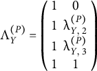 and
${\Lambda}_Y^{(G)}=\left(\begin{array}{cc}1& 0\\ {}1& {\unicode{x3bb}}_{Y,2}^{(G)}\\ {}1& {\unicode{x3bb}}_{Y,3}^{(G)}\\ {}1& 1\end{array}\right)$
and
${\Lambda}_Y^{(G)}=\left(\begin{array}{cc}1& 0\\ {}1& {\unicode{x3bb}}_{Y,2}^{(G)}\\ {}1& {\unicode{x3bb}}_{Y,3}^{(G)}\\ {}1& 1\end{array}\right)$
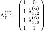 . We fixed
${\unicode{x3bb}}_{Y,1}^{(P)}={\unicode{x3bb}}_{Y,1}^{(G)}=0$
. We fixed
${\unicode{x3bb}}_{Y,1}^{(P)}={\unicode{x3bb}}_{Y,1}^{(G)}=0$
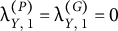 and
${\unicode{x3bb}}_{Y,4}^{(P)}={\unicode{x3bb}}_{Y,4}^{(G)}=1$
and
${\unicode{x3bb}}_{Y,4}^{(P)}={\unicode{x3bb}}_{Y,4}^{(G)}=1$
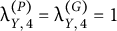 , while
${\unicode{x3bb}}_{Y,t}^{(P)}$
, while
${\unicode{x3bb}}_{Y,t}^{(P)}$
 and
${\unicode{x3bb}}_{Y,t}^{(G)}$
and
${\unicode{x3bb}}_{Y,t}^{(G)}$
 for
$t=2$
for
$t=2$
 and
$3$
and
$3$
 were freely estimated (Bollen & Curran, Reference Bollen and Curran2006, p. 102). In this specification,
${\unicode{x3bb}}_{Y,t}^{(P)}$
were freely estimated (Bollen & Curran, Reference Bollen and Curran2006, p. 102). In this specification,
${\unicode{x3bb}}_{Y,t}^{(P)}$
 and
${\unicode{x3bb}}_{Y,t}^{(G)}$
and
${\unicode{x3bb}}_{Y,t}^{(G)}$
 represent the proportion of change at each time point relative to the total change from the first to the final time point (Bollen & Curran, Reference Bollen and Curran2006, p. 102). This specification allows alternative representations of individual- and group-level nonlinear growth trajectories. Based on this model, we can examine which type of growth trajectory provides a useful representation the development of this academic proficiency development during elementary school.
The prior distribution of
${\unicode{x3bb}}_{Y,t}^{(P)}$
 and
${\unicode{x3bb}}_{Y,t}^{(G)}$
and
${\unicode{x3bb}}_{Y,t}^{(G)}$
 for
$t=2$
for
$t=2$
 and
$3$
and
$3$
 was specified as
$N\left(1,1\right)$
was specified as
$N\left(1,1\right)$
 . The DCM component was based on the LCDM with a random effect, which showed the best fit in the previous analysis. The structural model specification was the same as that of the previously selected best-fitting model. The MCMC settings were also unchanged from the previous analysis. The same data set as in the previous section was used. Detailed model specifications are provided in the R code available on the OSF webpage.
The WAIC value was
$\mathrm{29,405.153}\;\left( SE=260.561\right),$
 which was not better than that of the previously selected best-fitting model shown in Table 15. However, the difference was small relative to the standard error. Thus, the freely estimated loading model did not improve model fit, and the results did not provide strong evidence favoring the more flexible growth specification. Nevertheless, we briefly examined the estimated loading values and structural parameters for descriptive purposes.
First, the posterior mean of
${\unicode{x3bb}}_{Y,2}^{(P)}$
 was
$0.583\left(95\%\mathrm{CI}\left[0.475,0.693\right]\right).$
was
$0.583\left(95\%\mathrm{CI}\left[0.475,0.693\right]\right).$
 This result suggests that the growth from third to fourth grade corresponded to 60% of the total person-level growth from third to sixth grade. Similarly, the posterior mean of
${\unicode{x3bb}}_{Y,3}^{(P)}$
This result suggests that the growth from third to fourth grade corresponded to 60% of the total person-level growth from third to sixth grade. Similarly, the posterior mean of
${\unicode{x3bb}}_{Y,3}^{(P)}$
 was
$0.955\left(95\%\mathrm{CI}\left[0.823,1.108\right]\right)$
was
$0.955\left(95\%\mathrm{CI}\left[0.823,1.108\right]\right)$
 , indicating that a substantial proportion of person-level growth had already occurred by fifth grade. These results suggest that person-level growth may exhibit slight nonlinearity. On the other hand
$, {\unicode{x3bb}}_{Y,2}^{(G)}$
, indicating that a substantial proportion of person-level growth had already occurred by fifth grade. These results suggest that person-level growth may exhibit slight nonlinearity. On the other hand
$, {\unicode{x3bb}}_{Y,2}^{(G)}$
 was estimated as
$0.275\;\left(95\%\mathrm{CI}\left[0.249,0.298\right]\right)$
was estimated as
$0.275\;\left(95\%\mathrm{CI}\left[0.249,0.298\right]\right)$
 , and
${\unicode{x3bb}}_{Y,3}^{(G)}$
, and
${\unicode{x3bb}}_{Y,3}^{(G)}$
 was estimated as
$0.566\left(95\%\mathrm{CI}\left[0.535,0.596\right]\right)$
was estimated as
$0.566\left(95\%\mathrm{CI}\left[0.535,0.596\right]\right)$
 . These estimates suggest that group-level growth was relatively close to linear growth.
Finally, the estimates of the structural model parameters were shown in Table 20. The parameter estimates for the intercept factor were similar to those shown in Table 18. Because the scale of the slope factor changed under the freely estimated loading specification, the magnitudes of the slope-related structural parameters also changed, although the substantive interpretation remained largely similar. Specifically, the main effect of Attribute 2,
${\unicode{x3b3}}_2^{(P)}=-0.661\;\left(95\%\mathrm{CI}\left[-1.148,-0.091\right]\right)$
 , and the interaction effect between Attributes 2 and 3,
${\unicode{x3b3}}_{23}^{(P)}=0.866\;\left(95\% \mathrm{CI}\left[0.250,1.457\right]\right)$
, and the interaction effect between Attributes 2 and 3,
${\unicode{x3b3}}_{23}^{(P)}=0.866\;\left(95\% \mathrm{CI}\left[0.250,1.457\right]\right)$
 , were approximately three times larger than those reported in Table 18.
Parameter estimates of the structural model part in freely estimated slope loading model

Table 20 Long description
The table is divided into two main sections: Person level and Group level.
At the Person level, six parameters are listed with their Intercept (Mean and 95% C I) and Slope (Mean and 95% C I):
* Main effect of attribute 1 (gamma sub 1 super P): Intercept Mean 0.861 (0.644, 1.089); Slope Mean minus 0.066 (minus 0.361, 0.203).
* Main effect of attribute 2 (gamma sub 2 super P): Intercept Mean 0.910 (0.507, 1.242); Slope Mean minus 0.661 (minus 1.148, minus 0.091).
* Main effect of attribute 3 (gamma sub 3 super P): Intercept Mean 0.395 (0.140, 0.645); Slope Mean minus 0.007 (minus 0.311, 0.295).
* Interaction effect of attributes 1 and 3 (gamma sub 13 super P): Intercept Mean 0.094 (minus 0.193, 0.387); Slope Mean 0.260 (minus 0.102, 0.626).
* Interaction effect of attributes 2 and 3 (gamma sub 23 super P): Intercept Mean minus 0.308 (minus 0.752, 0.156); Slope Mean 0.866 (0.250, 1.457).
* Interaction effect of attributes 1 to 3 (gamma sub 123 super P): Intercept Mean minus 0.231 (minus 0.487, 0.095); Slope Mean 0.036 (minus 0.301, 0.361).
At the Group level:
* Effect of random intercept (gamma super G): Intercept Mean minus 1.422 (minus 2.127, minus 0.922); Slope Mean 2.190 (1.483, 3.136).
Bolded values indicate statistical significance where the 95% C I does not cross zero.
In summary, this additional analysis illustrates that the current RDC–MGC formulation can accommodate alternative trajectory specifications within the same longitudinal modeling setting while preserving the substantive interpretation of the relationship between attribute mastery and later growth trajectories.
6 Discussion and future study
This study proposed an RDC–MGC model, which assumes a random intercept for the DCM, a multilevel structure for the GC model, and a structural model linking the DCM and GC model. The primary purpose of the proposed model is to examine how diagnostic information relates to later developmental trajectories while accounting for multilevel data structures. The RDC–MGC model accounts for a group-level difference in the diagnostic test while also distinguishing between individual- and group-level mathematical ability growth. This feature enables the model to reveal the individual-level relationship between attribute mastery and growth, with the structural component representing the pure relationship between attribute mastery and individual growth. Two simulation studies showed that the two-level model with Bayesian estimation method provided smaller absolute biases and RMSEs and more appropriate coverages of 95% CI than single-level models. Real-data analysis demonstrated that the RDC–MGC model is more appropriate than single-level models. The parameter estimates indicated that attribute mastery at the second grade affected both the intercept and slope of mathematics ability from the third to sixth grades. A freely estimated loading specification, which represents a modification of the basic RDC–MGC model, was estimated to illustrate an alternative growth trajectory specification.
This study aimed to develop a model for controlling group-level effects and improving the effect of mastery of attributes on longitudinal growth. The proposed model interpreted the attribute mastery effects as individual effects, a concept that has not been addressed in previous studies. The real-data analysis demonstrated that basic attributes such as understanding of mathematical procedures or calculation skills predicted the individual-level growth during the later period of elementary school. In other words, cognitive abilities that ought to be mastered during the early period of elementary school could be identified. In addition to such empirical findings, the proposed model can be applied to other disciplines, such as language learning. Therefore, the proposed model can facilitate studies on the relationship between attribute mastery and its effects on subsequent ability growth.
The real-data example showed the effects of attribute mastery on both the intercept and slopes. Unlike
${\unicode{x3b3}}_S^{(P)}$
 s,
${\unicode{x3b3}}_I^{(P)}$
s,
${\unicode{x3b3}}_I^{(P)}$
 s can be interpreted easily. In our data analysis, calculation skills had a positive effect, whereas a deep understanding of mathematical procedures had a contradictory effect on the slope.
First, the positive effect of calculation skills may indicate that calculation is a core skill for elementary school-level arithmetic ability. Calculation is essential for achieving high test scores in arithmetic and can also alleviate cognitive burdens when students learn more complex mathematical concepts or procedures. Furthermore, calculation skills may help maintain students’ motivation to learn mathematics. In other words, calculation test items can serve as an enjoyable puzzle for students with strong calculation skills. This explains why calculation skills have a positive effect.
Second, the negative effect of a deep understanding of mathematical procedures is more challenging to interpret. In cognitive psychology, a deep understanding of mathematical procedures is generally considered beneficial. However, focusing excessively on understanding the meaning of mathematical procedures may limit the time available for practicing calculation skills. As aforementioned, calculation skills dominate elementary school mathematics, and students who prioritize deep understanding over calculation practice may fail to develop their calculation abilities, negatively impacting their test scores. This does not suggest that calculation practices should be performed without understanding; rather, a balance is necessary.
Several additional explanations might be possible. Mastering only “deep understanding” did not sufficiently represent a deep understanding of mathematical procedures. Although this is confusing, mastering only “deep understanding” indicates that students could talk about the concept or meaning of the mathematical procedures but could not apply the knowledge to solve real mathematical problems. An appropriate “deep understanding” referred to mastering calculation procedures and understanding their meaning. This involved mastering both A2 and A3 attributes. Therefore, the estimation result revealed a problematic mastering pattern. Because of a lack of calculation skills, students who had only mastered “deep understanding” could not appropriately use procedural knowledge to solve mathematical problems, and this slowed the growth of general academic proficiency that was primarily represented as mathematical problem-solving ability, including calculation skills, in this study.
We analyzed the effect of mastering deep understanding on the individual intercept parameter and obtained a value of 0.913, which is the highest among the three attributes (see Table 15). In the third grade, some students might master a deeper understanding higher level than just mastering calculation, and they indicated higher initial scores in the third grade. However, students mastering only “deep understanding” neglected calculation. This meant there might be some heterogeneity in mastering “deep understanding.” Using the item measuring the A2 attribute, students can connect procedures to concrete examples or diagrammatic representations; however, calculation is still important during the elementary school period. Therefore, although deep understanding is crucial for learning, the findings of this study suggest some conditions for such deep understanding.
Another consideration is that students might think they deeply understand the procedure, thus ignoring repetitive procedural practice, such as drill-like procedural exercises, in a learning situation. Similarly, an excessive focus on semantic understanding may increase the cognitive load for test items, and the procedures have not become automatic. This can result in overthinking, limiting the student’s ability to solve test items and consequently reducing growth rate.
The positive interaction effect of a deep understanding of mathematical procedures and calculation on the slope compensated for the negative effect of a deep understanding of mathematical procedures. The interaction effects of A2 and A3 are understandable because previous studies have emphasized the necessity of both procedural and conceptual understanding (Rittle-Johnson, Reference Rittle-Johnson, Dunlosky and Rawson2019, for a review). Furthermore, adaptive learners do not persist in a deeper procedure and can use a shallow procedure (Star, Reference Star2005; Star & Rittle-Johnson, Reference Star and Rittle-Johnson2008). This interpretation is consistent with the literature. The estimated positive effect was greater than the negative effect. Therefore, students who learned both attributes tended to grow faster than those who mastered only one of the two attributes. This suggests that the benefits of deep understanding of mathematical procedures may be more likely to emerge when accompanied by sufficient calculation skills. A deep understanding of procedures is crucial for comprehending higher-level mathematical concepts. Our data analysis shows that during elementary school, both understanding and calculation skills must be balanced. They are complementary and both are important to appropriately improve mathematical ability.
This study has several limitations. First, the parameter estimation of the RDC–MGC model is computationally intensive. Our setting required several hours to complete necessary iterations. Furthermore, the large number of model parameters necessitates significant memory capacity on our computer. Therefore, more computationally efficient estimation methods, such as variational inference (Cho et al., Reference Cho, Wang, Zhang and Xu2021; Rijmen & Jeon, Reference Rijmen and Jeon2013; Yamaguchi, Reference Yamaguchi2023; Yamaguchi & Martinez, Reference Yamaguchi and Martinez2024; Yamaguchi & Okada, Reference Yamaguchi and Okada2020) or stochastic optimization techniques (Cai, Reference Cai2010a, Reference Cai2010b; Robbins & Monro, Reference Robbins and Monro1951; von Davier & Sinharay, Reference von Davier and Sinharay2010; Zhang et al., Reference Zhang, Chen and Liu2020), are required.
Second, developing a diagnostic test and vertically scaled tests is challenging. Moreover, collecting data for these tests is not straightforward. However, the use of computers in classrooms may facilitate data collection and enhance the extension of this model.
Third, our dataset lacks covariates at both the person and group levels. If covariates were available, they could be used to explain the variance in intercepts and slopes within the proposed model. Furthermore, these covariates could help identify factors that influence individual growth beyond attribute mastery. For instance, teachers’ teaching strategies (Carbonneau et al., Reference Carbonneau, Marley and Selig2013), students’ learning strategies (Aleven & Koedinger, Reference Aleven and Koedinger2002), and motivation (Metallidou & Vlachou, Reference Metallidou and Vlachou2007) could all be important factors to assess in future research.
It may be beneficial to consider applicable fields of the RDC–MGC model for future study. Basically, the RDC–MGC model is intended to examine later growth using diagnostic mastery status. Keeping this structure in mind, we can change the diagnostic part. Some DCMs can reveal students’ misconceptions (e.g., Kuo et al., Reference Kuo, Chen and de la Torre2018; Ozaki et al., Reference Ozaki, Sugawara and Arai2019); therefore, we can assess what kind of misconceptions and their combination influence the subsequent growth of academic proficiency. For example, Kuo et al. (Reference Kuo, Chen and de la Torre2018) assumed three misconceptions in the fraction multiplication test in elementary school: “turning the second fraction upside down when multiplying a fraction by a fraction,” “solving only the first step of a two-step problem,” and “performing incorrect arithmetic operations when confused about the relational terms.” These misconceptions may prevent later mathematical learning. Ozaki et al. (Reference Ozaki, Sugawara and Arai2019) analyzed two misconceptions in the Reading Skill Test in Japanese: “in which the nearest word is the subject” and “in which the word beginning a sentence is the subject.” These are the basics of reading text and may result in deficiency in reading proficiency. Researchers may be interested in the interaction effects of misconceptions on subsequent learning achievement and overall learning growth.
Furthermore, DCMs have been employed for non-academic contexts such as clinical psychology, which may be an interesting application field of the RDC–MGC model. Templin and Henson (Reference Templin and Henson2006) applied DCMs to psychological assessment. Wang et al. (Reference Wang, Gao, Cai and Tu2019) developed a depression diagnostic measure with DCMs, and Bao et al. (Reference Bao, Liu, DiStefano and Ding2025) applied DCMs for the behavioral and emotional problems of children. Liang et al. (Reference Liang, de la Torre, Larimer, Mun, Stemmler, Wiedermann and Huang2024) identified mental health symptom profiles of college students, and de la Torre et al. (Reference de la Torre, van der Ark and Rossi2017) analyzed data from the Dutch version of Millon Clinical Multiaxial Inventory-III which measures multiple psychological disorders. Those diagnostic results can be predictors of later psychological latent GCs. For example, the GC model has been employed for school or clinical psychology: self-efficacy beliefs in regard to anger and sadness regulation during adolescence (Di Giunta et al., Reference Di Giunta, Lunetti, Lansford, Eisenberg, Pastorelli, Bacchini, Tirado, Iselin, Basili, Gliozzo, Favini, Cirimele and Remondi2023), adolescent depressive symptom changes (Gataviņš et al., Reference Gataviņš, Visoki, Hoffman, Almasy and Barzilay2025), developmental change in mental problems, such as stress or anxiety during college (Liu et al., Reference Liu, Zhang, Gao and Cao2023), and so on. Based on those studies, diagnoses of mental problems can be used to examine how they affect subsequent depression trajectories. Another possible application is examining how emotional problems affect children’s self-efficacy beliefs.
Although the current study has several limitations and the main objective of the RDC–MGC model is to predict later latent growth using diagnostic information, several possible extensions can be considered. Here, we discuss the future extensions. First, the measurement part can be changed to other DCMs. This is employed in the real-data analysis section. In addition, for the usual multilevel models (e.g., Raudenbush & Bryk, Reference Raudenbush and Bryk2002), the group-level variables can be included in the measurement model to explain group differences. Furthermore, the attribute effects can include random effects that are random slopes in the multilevel models.
Second, the GC model can be extended to the non-linear growth case. For example, quadratic or higher-order slope terms can be added, or some slope paths can be freely estimated (Bollen & Curran, Reference Bollen and Curran2006, Chapter 4); the latter specification was shown in the real-data analysis. Piecewise approach with unknown knots and its extensions can be used to capture critical change points in the learning trajectory (e.g., Kohli & Harring, Reference Kohli and Harring2013; Kohli et al., Reference Kohli, Harring and Hancock2013). Such growth functions can be assumed at both the individual and group levels. Furthermore, conditional latent curve models (Bollen & Curran, Reference Bollen and Curran2006, Chapter 5) enable us to incorporate additional time-invariant covariates. These are some possible extensions. Note that the growth period does not have to be as long as the empirical example in the manuscript. Assuming shorter periods, such as one year or less, may be appropriate for examining development within a school year. For example, if the diagnostic assessment is conducted at the first period of the school year, such information can be used to explain subsequent student growth.
Third, the structural part can also be changed. It is possible to assume nonlinear or polynomial regression functions. Furthermore, as mentioned above, group-level variables can also be introduced into the structural model, and nonlinear functions can be employed. For example, school type (public/private) or teachers’ teaching strategies are group-level factors and may improve students’ learning and result in higher slopes or intercepts. In addition, interactions among group-level predictors and attributes are cross-level interactions (e.g., Raudenbush & Bryk, Reference Raudenbush and Bryk2002, p. 29). Mediation variables can be inserted between the attributes and growth factors. This extension makes it possible to examine the mechanisms through which attributes improve individual learning. Furthermore, if an educational intervention is conducted based on the diagnostic assessment, the treatment variable can be included in the structural model.
As a different perspective, we can set attribute mastery as the final outcome and use growth models as explanatory variables. This is not a minor modification of the RDC–MGC model, but the important part is that the proposed model is based on the combination of DCMs, SEM, and multilevel models. Therefore, various research questions can be examined using the extended model. The extensions of the proposed method are relatively straightforward.
The utility of the above models should ultimately be evaluated by using empirical datasets in future studies. Generally, statistical methods are tailored for specific purposes, so the simplest RDC–MGC model can only address limited educational research questions. However, because the RDC–MGC model is composed of DCMs, multilevel modeling, and SEM, each element can be modified for various study objectives.
Supplementary material
To view supplementary material for this article, please visit http://doi.org/10.1017/psy.2026.10126.
AI use declaration
During the preparation and revision of this manuscript, the authors used ChatGPT (OpenAI, GPT-5.5) to assist with English language editing, grammar checking, and refinement of academic writing. All AI-generated outputs were reviewed and edited by the authors, who take full responsibility for the content of the manuscript.
Data availability statement
The data analysis code is available on the Open Science Framework page: https://osf.io/gpztw. We appreciate Tokyo Shoseki Co. for providing the real data.
Funding statement
This work was supported by JSPS KAKENHI 20H01720, 22K13810, 23H00985, 23H00065, 23K20759, 24K00485, and 25K17133.
Competing interests
The authors declare no competing interests.
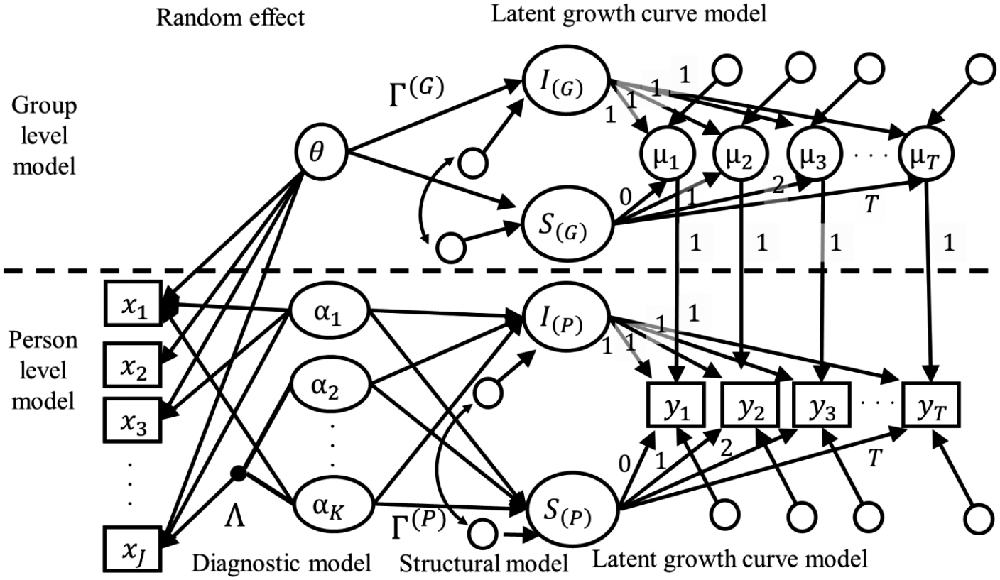
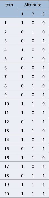
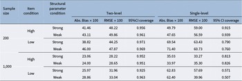

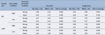

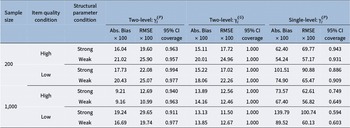


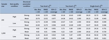


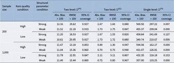


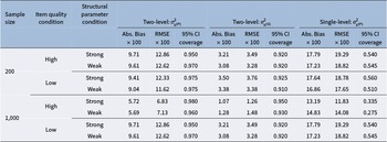


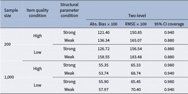


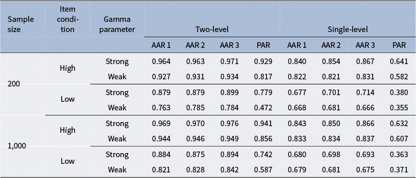
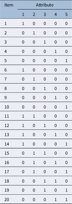

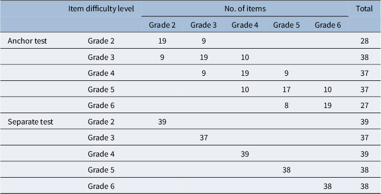
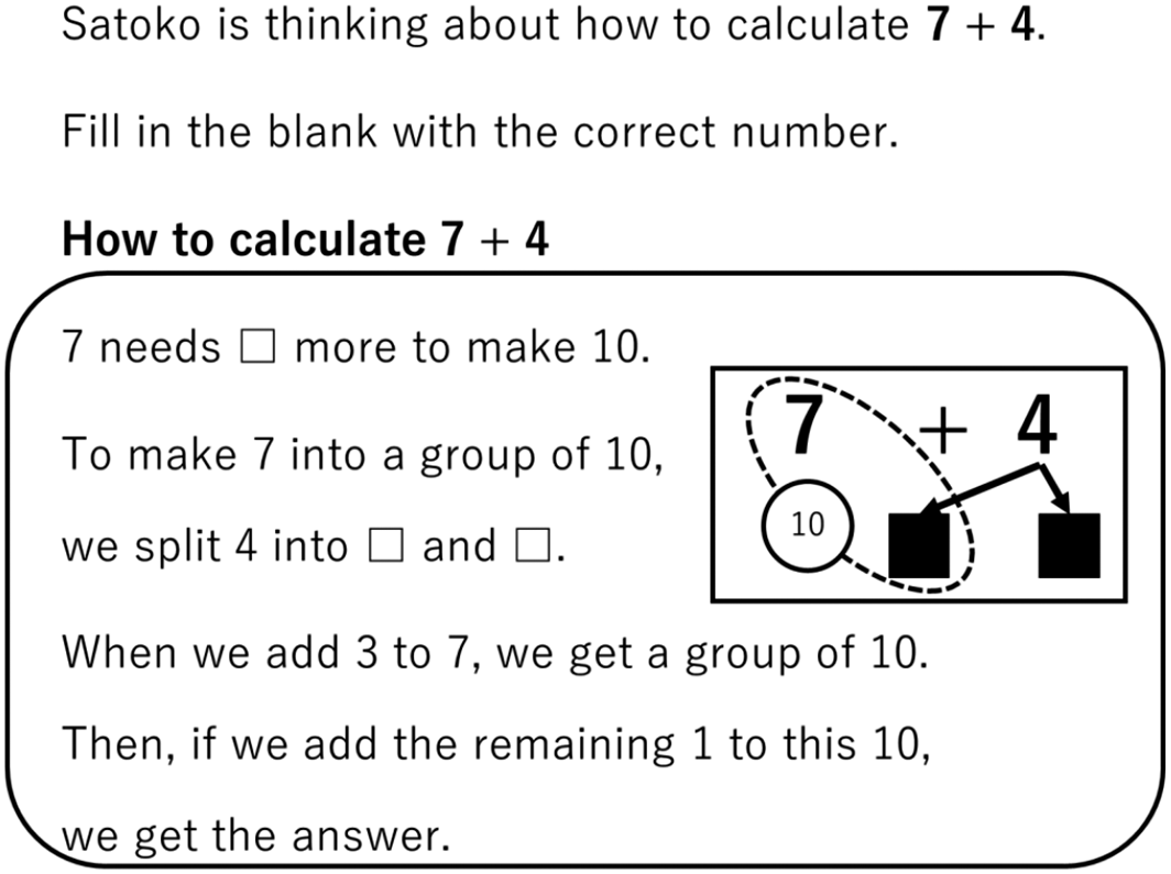
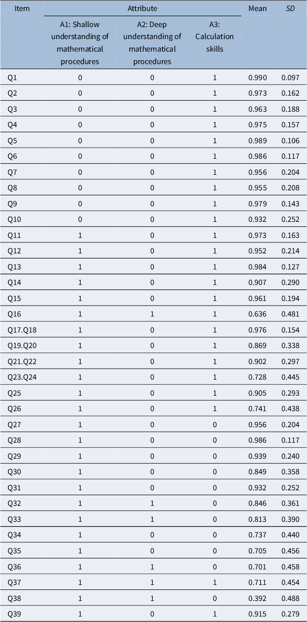
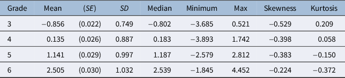
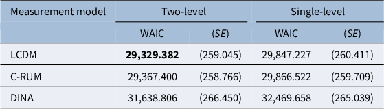
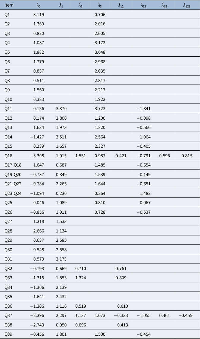
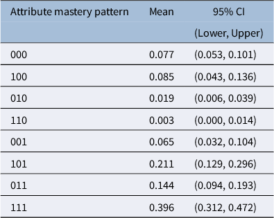
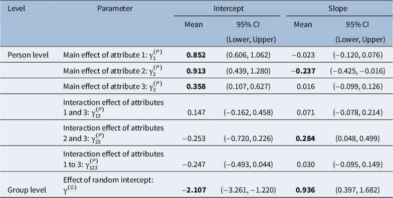
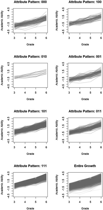
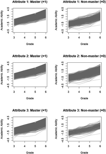
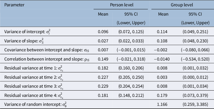
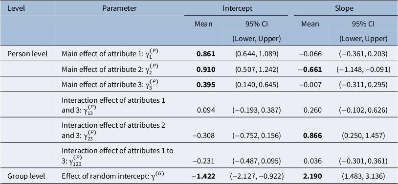


 Open access

