

1. Introduction
Continuous mass/energy-balance measurements and the repeated compilation of glacier inventory data are two end members of modern integrated glacier-observing systems (Reference Haeberli, Hoelzle and ZempWGMS, 2007; Reference Zemp, Paul, Hoelzle, Haeberli, Orlove, Wiegandt and LuckmanZemp and others, 2008). The interpretation of mass- and energy-balance measurements provides the basic process understanding of climate/glacier interactions and enables the development of corresponding numerical models to inter- and extrapolate the few measured values to regions and periods without such detailed measurements. Glacier inventories contain the basic regional data to accomplish this task (Reference Haeberli and HoelzleHaeberli and Hoelzle, 1995; Reference Hoelzle, Chinn, Stumm, Paul and HaeberliHoelzle and others, 2007).
The increasing availability of high-resolution digital terrain models (DTMs) now opens promising perspectives to more directly relate mass-balance measurements to regional glacier information and large samples of glaciers (Reference Machguth, Paul, Hoelzle and HaeberliMachguth and others, 2006, Reference Machguth, Paul, Kotlarski and Hoelzle2009). This kind of data combination represents an important step towards the direct coupling of a mass-balance model applied to numerous glaciers with climate model output (e.g. Reference Machguth, Paul, Kotlarski and HoelzleMachguth and others, 2009; Reference Paul and KotlarskiPaul and Kotlarski, 2010), even though the uncertainties involved are considerable (Reference Machguth, Purves, Oerlemans, Hoelzle and PaulMachguth and others, 2008). Furthermore, it opens up the opportunity to model key glacier mass-balance parameters for numerous glaciers from a synthetic mass-balance network. The present paper makes a first attempt in this direction.
Certain parameters derived from direct glacier mass-balance measurements are good indicators of glacier characteristics as a function of climatic conditions. The equilibrium-line altitude (ELA), the accumulation-area ratio (AAR) and both parameters for a zero mass balance (ELA0, AAR0) are, for instance, regularly reported in the Glacier Mass Balance Bulletin of the World Glacier Monitoring Service (Reference Haeberli, Gartner-Roer, Hoelzle, Paul and ZempWGMS, 2009, and earlier issues). From the graphs in these publications, the mass-balance gradient (Γ) and the balance rate at the terminus (b t) can be derived. The first is the primary link between average atmospheric conditions, glacier mass turnover and flow. The latter relates to the dynamic response (length change, adaptation to new equilibrium) of glaciers (Reference Jóhannesson, Raymond and Waddingtonjóhannesson and others, 1989). Much earlier studies related mean air temperature at the ELA (TELA) to the precipitation regime (Reference AhlmannAhlmann, 1924; Reference Kotlyakov and KrenkeKotlyakov and Krenke, 1982) and hence to maritime- and continental-type glaciers with their strongly different activity/mass turnover, englacial temperatures and relations to periglacial permafrost and timberline (Reference ShumskiyShumskiy, 1964; Reference Haeberli and BurnHaeberli and Burn, 2002). In fact, such parameters have proved very useful for analyzing local-topographic to large- scale climatic characteristics of glacier distribution and mass balance (Reference Furbish and AndrewsFurbish and Andrews, 1984; Reference Ohmura, Kasser and FunkOhmura and others, 1992; Reference Dyurgerov and BahrDyurgerov and Bahr, 1999), for application to unmeasured glaciers (Reference Haeberli and HoelzleHaeberli and Hoelzle, 1995; Reference Hoelzle, Chinn, Stumm, Paul and HaeberliHoelzle and others, 2007; Reference Braithwaite and RaperBraithwaite and Raper, 2009), as well asfor paleoglaciological reconstructions (e.g. Reference Haeberli and AleanHaeberli and Penz, 1985; Reference Kerschner, Kaser and SailerKerschner and others, 2000).
Deriving such general parameters from field observations is laborious and only possible for a few glaciers with long enough mass-balance series. Besides the problem that the small data basis from observations limits the possibilities of statistically sound interpretations, mass-balance measurements also have their sources of uncertainty (e.g. Reference AndreassenAndreassen, 1999; Reference Fountain and VecchiaFountain and Vecchia, 1999). It is therefore desirable to have additional estimates of mass-balance parameters. To accomplish this, we present results for the Swiss Alps obtained from distributed modeling of a synthetic network of mass-balance glaciers. The mass-balance parameters are derived from the model output, with the experiment being run for balanced-budget conditions and 94 selected Swiss glaciers (Fig. 1), which is much more than the number of glaciers documented by field observations. Furthermore, the output of the spatially distributed model does not require interpolations to the entire glacier as is necessary from stake measurements; thus the synthetic network can be seen as an indirect alternative to the direct way of analyzing measurements. The work presented here, however, is highly experimental and complementary to the irreplaceable direct in situ measurements. It introduces new uncertainties and difficulties that require careful analysis and comparison to previous studies and measurements.
Model domain with the full DTM. Selected glaciers are in white and theremaining glaciers in dark gray. Crosses denote the centers of the REMO gridboxes. White dots show locations of the MeteoSwiss weather stations used for bias correction (altitude in ma.s.l.): COV = Corvatsch (3315); DAV = Davos (1590); EVO = Evolène (1825); GRI = Grimsel-Hospiz (1980); GSB = Grand St Bernard (2472); GUE = Gütsch (2287); JUF = Jungfraujoch (3580); MOL = Molèson (1972); PIL = Pilatus (2106); ROB = Robiei (1898); SAM = Samedan (1705); SAN = S?ntis (2490); WFJ = Weissfluhjoch (2690); and ZER = Zermatt (1638). For orientation, the Swiss border is shown as a solid line and lakes in light gray. The rectangular box indicates the area shown in Figure 4.

2. Basic Approch
A simplified distributed energy-balance model is applied to alculate the mass-balance distribution from which mass-balance parameters are derived. The design of the mass-balance model excludes any reference to the later derived mass-balance parameters. The model strictly operates on a grid and computes mass balance for each gridcell based on a number of input data, namely a DTM, the glacier perimeter and meteorological data.
In the present work, it is assumed that each glacier has a balanced-budget mass balance and an equilibrium extent. Though such a state is very rare in reality, it is nevertheless assumed here because (1) it is an important theoretical concept in glaciology (e.g. Reference Furbish and AndrewsFurbish and Andrews, 1984) and (2) it eases the validation and interpretation of the results. To make this assumption a less theoretical approximation, a model time frame (1970–85) is chosen where glaciers were actually close to a balanced-budget mass balance (Reference Haeberli, Gartner-Roer, Hoelzle, Paul and ZempWGMS, 2009). Only the cumulative mass balance (Σ Ba) over the entire time frame is assumed to be balanced; interannual variability of mass balance, including positive and negative years, still exists.
Modeled mean annual mass-balance distribution is analyzed with respect to the following mass-balance parameters: ELA, TELA, summer (June, July and August) air temperature (Ts,ELA), precipitation (PELA), accumulation calculated over an entire mass-balance year (AccELA), global radiation (Sin,ELA) at the ELA, AAR, bt and Γ. In the literature, parameters referring to a balanced-budget mass balance are usually written with the suffix 0 (e.g. ELA0, AAR0; cf. Reference CogleyCogley and others, 2011). Here all parameters refer to a balanced budget, so the suffix is omitted. Finally, the mass-balance parameters are analyzed with respect to topographic glacier parameters, in particular: surface area (A), minimum and maximum glacier altitude as well as elevation range of the glacier (zmin, zmax and Δz, respectively), a simple glacier hypsometry index (H) representing the ratio in width between accumulation and ablation area and median (zmed) as well as mid-range (zmid) glacier elevation.
3. Test Site and Data
The present study is performed for the Swiss Alps (Fig. 1), an area of ∼25 000 km2 including a glacierized area of ∼1340 km2 in 1973 (Reference Müller, Caflisch and MullerMüller and others, 1976). The DTM used is from Swisstopo, down-sampled from originally 25m to 100mresolution and referring approximately to the glacier surfaces in the mid-1980s. The digitized glacier outlines from the Swiss Glacier Inventory of 1973 (Reference PaulPaul, 2007) are used to distinguish ice-free from ice-covered areas, as well as individual ice bodies. Though some fast-reacting mid-sized mountain glaciers advanced over this period, the overall area changes were small (Reference Paul, Kääb, Maisch, Kellenberger and HaeberliPaul and others, 2004). This justifies the assumption that the 1973 glacier outlines and surface are valid for the entire calculation period.
Simplifications in the model make it impossible to calculate reasonable mass-balance values for all types of glaciers (see Section 4). Consequently, the analysis of mass-balance parameters is performed only for glaciers where reasonable mass-balance values are expected. These glaciers are selected based upon the following conditions: (a) no or little debris cover, (b) no or little influence of avalanches, (c) mass loss restricted to melting and (d) sufficient size (area
>1km2). A set of 94 glaciers were found to meet these conditions. The selected glaciers cover 610 km2, ∼50% of the total glacierized area. The mass-balance model is driven from output of the regional climate model (RCM) REMO (Reference JacobJacob and others, 2001). REMO is chosen because it was previously applied to drive glacier mass-balance models (Reference Machguth, Paul, Kotlarski and HoelzleMachguth and others, 2009; Reference Paul and KotlarskiPaul and Kotlarski, 2010), and biases in modeled highmountain climate are analyzed in depth by Reference Kotlarski, Paul and JacobKotlarski and others (2010). We use data from an RCM run for 1958–2003, at a spatial resolution of 1/6? (∼18 km) and forced by ERA-40 as well as the operational European Centre for Medium-RangeWeather Forecasts (ECMWF) reanalysis at the boundaries. For RCM bias correction (T and Sin), meteorological observations from 14 high mountain weather stations (Fig. 1) operated by MeteoSwiss are applied. For correction of the precipitation bias, the gridded (∼2 km resolution) precipitation climatology by Reference Schwarb, Daly, Frei and ScharSchwarb and others (2001) is used. For validation of modeled mass balance we use annual (B a; 1 October–30 September), winter (B w; 1 October–30 April) and summer balance (Bs; 1 May–30 September) calculated for 50 Swiss glaciers by a combined approach of modeling and measurements (Reference Huss, Hock, Bauder and FunkHuss and others, 2010a, Reference Huss, Usselmann, Farinotti and Bauderb), as well as observed B a for nine Alpine glaciers (Reference Haeberli, Hoelzle and ZempWGMS, 2007).
4. Methods
4.1. The mass-balance model
The applied glacier mass-balance model is a simplified version of more sophisticated energy-balance approaches. Here we briefly summarize the model; a detailed description is given by Reference Machguth, Paul, Kotlarski and HoelzleMachguth and others (2009).
The model runs at daily steps, and the cumulative mass balance b c on day t + 1 is calculated for every time-step and over each gridcell of the DTM according to Reference OerlemansOerlemans (2001):
where t is the discrete time variable, Δt is the time-step (86 400 s=1 day), l m is the latent heat of fusion of ice (334 kJ kg−1) and P solid is solid precipitation (mw.e.). The energy available for melt (Q m) is calculated as follows:
where α is the albedo of the surface, S in is the global radiation, T is the air temperature (°C) at 2m above ground and outside the glacier boundary layer, and C 0 + C 1 T is the sum of the longwave radiation balance and the turbulent exchange linearized around the melting point (Reference OerlemansOerlemans, 2001). In contrast to Reference Machguth, Paul, Kotlarski and HoelzleMachguth and others (2009), bias-corrected RCM data are used to force the model and the calibration of the model is re-evaluated. The calibration is restricted to summer melt since winter mass balance is adjusted iteratively by varying P during the model run as explained in Section 4.3. Best fit of observed and modeled melt during the summer months on 14 Swiss glaciers (Reference Machguth, Paul, Kotlarski and HoelzleMachguth and others, 2009) was achieved at C1 = 12 W m-2 K-1 and C0 = -45Wm-2.
The source of accumulation is precipitation (P), and a threshold temperature (T snow) of 1.5°C in combination with a transition range of 0.5°C (i.e. linear increase of the rain fraction from 0% at 1 °C to 100% at 2°C) is used to distinguish P solid from rain. Redistribution of snow by wind or avalanches is not considered in the model. Refreezing is also not taken into account (it plays a minor role in the European Alps) and any meltwater and rainfall is immediately removed from the glacier.
Global radiation (S in) is calculated from potential clear- sky global radiation (S in,clr) and cloudiness (n). The latter is acquired from the RCM output on a daily basis, whereas S in,clr is computed in a preprocessing routine according to Reference IqbalIqbal (1983) and Reference CorripioCorripio (2003), considering all effects of surface topography including shading and assuming standard atmospheric transmission coefficients for clear-sky conditions. S in,clr is the sum of diffuse (S in,clrdir) and direct radiation (S in,clrdir) which are both preprocessed from the DTM and stored subsequently as 2 × 365 arrays (extent and resolution identical to the DTM) of daily mean S in,clrdir and S in,Clrdir. During the mass-balance model run, S in of every individual time-step is computed from the corresponding preprocessed grids S in,clrdif and S in,clrdir and attenuation of clouds (τcl). The latter is derived from the RCM cloudiness at the actual time-step according to τcl = 1.0 - 0.233n - 0.415n 2 (Reference Greuell, Knap and SmeetsGreuell and others, 1997).
Glaciers are regarded as debris-free, and depending on the surface characteristics (snow, firn or ice) three different constant values for the surface albedo are used in the model: αs = 0.72, αf = 0.45 or αi = 0.27. While the firn albedo has little influence on the model results, the values chosen for αs and αi resulted in good agreement of model results and observations (Reference Machguth, Paul, Kotlarski and HoelzleMachguth and others, 2009) and are thus also used in this study. Accumulated snow is assigned af when its age exceeds 1 year, and after 2 years its albedo is lowered to α i.
4.2. Downscaling of the RCM data and bias correction
The spatial resolution of the RCM and that of the mass-balance model differ greatly, so the RCM data are downscaled for the mass-balance calculation. The downscaling procedure comprises two steps: (1) the RCM data are interpolated to the resolution of the DTM using interpolation techniques, followed by (2) the application of subgrid parameterizations. A detailed description of both steps as well as a brief theoretical background are given by Reference Machguth, Paul, Kotlarski and HoelzleMachguth and others (2009). The key tasks in step 1 are, on the one hand, to choose interpolation schemes that generate smooth changes from one RCM gridcell to the next because such a pattern is more realistic than abrupt breaks from one gridbox to the next. On the other hand, characteristics of the RCM data, such as mean values and frequencies of events of different magnitude (e.g. wet-day frequency), should be preserved. Through experiments and theoretical considerations, Reference Machguth, Paul, Kotlarski and HoelzleMachguth and others (2009) found that thin- plate splines (TPS) interpolation performs best with respect to the aims of step 1. Consequently, TPS is used here to interpolate at each time-step the corresponding daily RCM fields of T, P and n to the DTM resolution. Prior to the interpolation of T the strong dependence on altitude is removed by reducing T to a standard altitude H0 = 0 m a.s.l. by means of a temporally and spatially constant altitudinal gradient (atmospheric lapse rate) γT = -0.0065 °Cm-1. As shown in more detail by Reference Machguth, Paul, Kotlarski and HoelzleMachguth and others (2009), the chosen value of γT agrees well with the mean RCM lapse rate and is in good agreement with near-surface summer lapse rates in the European Alps (Reference RollandRolland, 2003). No reduction to a standard altitude is performed for P and n because the RCM data show no significant dependence on altitude.
In step 2, simple subgrid parameterizations are applied to account for the major components of the small-scale influences of the rugged Alpine topography. The influence on T, P and S in, however, differs, so individual subgrid parameterizations are applied for these variables. In the following the subgrid parameterizations for T and Sin are addressed; the approach for P is explained in the next paragraph in connection with the de-biasing. Subgrid-scale variability of T is addressed by adjusting T from H 0 to the elevation of the DTM using the lapse rate γ T. The subgrid-scale variability of Sin is complex and mainly controlled by topographic effects like slope, exposition and shading. Cloudiness also exhibits a strong influence on Sin, but is distributed rather smoothly in space, in particular when daily means or longer time-spans are considered. Hence, the preprocessed grids of clear-sky global radiation account for the topographic subgrid-scale variability while the influence of cloudiness is derived directly from the interpolated fields of n and considers the temporal variability. Full details of the method, including a comparison to Sin modeled by the RCM, are given by Reference Machguth, Paul, Kotlarski and HoelzleMachguth and others (2009).
The downscaled RCM fields require additional bias correction for accurate mass-balance calculations (Reference Machguth, Paul, Kotlarski and HoelzleMachguth and others, 2009). Consequently we developed and applied specific approaches for bias removal in T, Sin and P. De-biasing of the downscaled fields of T and S in is based on comparison and adjustment to observations at the 14 high-mountain weather stations. Precipitation is corrected by scaling the precipitation field to match a high-resolution precipitation climatology Here we use the 2 km resolution precipitation map from Reference Schwarb, Daly, Frei and ScharSchwarb and others (2001) which is the most detailed currently available reference dataset based on records from >6000 rain gauges. Reference Schwarb, Daly, Frei and ScharSchwarb and others (2001) applied the interpolation method of Reference Daly, Neilson and PhillipsDaly and others (1994) to obtain spatially variable precipitation gradients (γ P ) from the rain-gauge records. Thus, the precipitation scaling provides at the same time the subgrid parameterization including γP (cf. step2 above) and the de-biasing. Full details of the bias correction methodology for all three variables are given in the Appendix.
4.3. Iterative precipitation adjustment
Despite all efforts to bias-correct model input, it is not possible to achieve satisfactory agreement with observed mass balances on a glacier-by-glacier basis. This is not only because we assume that all glaciers have an identical cumulative mass balance, but will also result when variability between the glaciers is considered: on the one hand, no current mass-balance model is able to capture all relevant processes; on the other hand, input variables are simply not known with sufficient accuracy. Even after bias correction, precipitation is considered the most uncertain variable because of the well-known difficulties in measuring solid precipitation in high-mountain environments (e.g. Sevruk, 1985, Reference Sevruk1997). Furthermore, previous studies using the Reference Schwarb, Daly, Frei and ScharSchwarb and others (2001) dataset for glacier mass-balance modeling found that at the elevation of glaciers the data require adjustment (e.g. Reference Zemp, Hoelzle and HaeberliZemp and others, 2007) by a factor of up to two (Reference Huss, Bauder and FunkHuss and others, 2009). Consequently, we decided to tune P to achieve 'observed' mass balance.
The precipitation adjustment is performed individually for each modeled glacier to achieve a cumulative mass balance of 0mw.e. over the calculation period. As already mentioned, only the cumulative mass balance for the period 1970-85 is forced to be zero; variability of annual mass balance still exists. The iterative precipitation adjustment starts with the calculation of cumulative mass balance in a first model run. For each glacier a first multiplicative precipitation adjustment (M P) is estimated by comparing model outcome to the assumed Σ B a = 0m w.e. Subsequently, after each iteration, MP is corrected until for each glacier a cumulative mass balance of 0mw.e. with a tolerance of ±0.2m w.e results.
4.4. Deriving topographic and glacier mass-balance parameters
The topographic glacier parameters A, z
min, z
max as well as Δz are derived from the DTM and the digitized glacier outlines at 100 m spatial resolution. Glaciers are divided into 50 m elevation bands (z
i) where the index i refers to the respective interval. Mid-range glacier elevation is defined as z
mid = (z
max - z
min)/2, and median glacier elevation as ![]() (Reference Haeberli, Bösch, Scherler, Østrem and WallenWGMS, 1989). Furthermore we calculate a simple hypsometry index (H) from the ratio of mean Ai
of the accumulation and ablation area. The latter two are divided by zmed because this parameter is highly correlated with the ELA (Reference Braithwaite and RaperBraithwaite and Raper, 2009) and using z
med makes the computation of H independent of prior knowledge of the mass-balance distribution. If there are fewer than five elevation bands in the accumulation or ablation area, H is not calculated. H is intended to be a first-order estimate of the ratio of glacier width in the accumulation and ablation areas; the higher H the stronger the difference in width. Thereby glacier width at a specific elevation i is approximated with A
i. A more accurate hypsometry index would require considering the surface slope, but here we prefer a simpler and more widely applicable index.
(Reference Haeberli, Bösch, Scherler, Østrem and WallenWGMS, 1989). Furthermore we calculate a simple hypsometry index (H) from the ratio of mean Ai
of the accumulation and ablation area. The latter two are divided by zmed because this parameter is highly correlated with the ELA (Reference Braithwaite and RaperBraithwaite and Raper, 2009) and using z
med makes the computation of H independent of prior knowledge of the mass-balance distribution. If there are fewer than five elevation bands in the accumulation or ablation area, H is not calculated. H is intended to be a first-order estimate of the ratio of glacier width in the accumulation and ablation areas; the higher H the stronger the difference in width. Thereby glacier width at a specific elevation i is approximated with A
i. A more accurate hypsometry index would require considering the surface slope, but here we prefer a simpler and more widely applicable index.
Mass-balance parameters are derived from the modeled grid of mean annual glacier mass-balance distribution at 100m spatial resolution. The AAR is calculated from the ratio of gridcells with positive and negative mass balance. Mass-balance profiles are defined by calculating mean mass balances for all z i. The ELA is defined as the elevation where the mass-balance profile equals 0 m w.e. Where this is true for more than one elevation, a mean value is calculated (this rare phenomenon is mainly induced by variability of solar radiation and can occur on steep north-facing glaciers with complex topography). Subsequently, all cells are selected that are located within ±25 m difference in elevation of the ELA, and meteorological conditions at these cells are averaged to obtain T ELA, P ELA, AccELA and S in,ELA. Mass-balance gradients for ablation and accumulation area (Γabl and Γacc, respectively) are calculated from linear regressions of the mean mass balances of the elevation bands, where the latter are weighted according to their areas. If there are fewer than five elevation bands in the accumulation or ablation area, the corresponding gradient is not calculated. Subsequently the balance ratio Γratio = Γabl/Γacc is calculated (Reference Furbish and AndrewsFurbish and Andrews, 1984). For the case that Γacc → 0, Γratio would become undefined. Since in this study Σ B a ≡ 0, Γacc are always greater than 0 (minimum value Γacc = 0.125) because otherwise ablation would not be balanced by accumulation. The balance rate at the tongue is derived from the regression function for Γabl and the elevation of the tongue (z t), where the latter is defined as the mean z of the lowest three elevation bands.
4.5. Validation of the synthetic glacier mass-balance network
In Figure 2a, modeled mean B s, B w and B a are compared to the mean measured mass balances of nine Alpine glaciers (Austria: Hintereisferner, Kesselwandferner, Sonnblickkees, Vernagtferner; France: Glacier de Saint-Sorlin, Glacier de Sarennes; Italy: Ghiacciaio del Careser; Switzerland: Griesgletscher, Silvrettagletscher; cf. Reference Haeberli, Hoelzle and ZempWGMS, 2007) and modeled mass balances for 50 Swiss glaciers (Reference Huss, Hock, Bauder and FunkHuss and others, 2010a, Reference Huss, Usselmann, Farinotti and Bauderb). Linear regressions of annual values from Reference Huss, Hock, Bauder and FunkHuss and others (2010a, Reference Huss, Usselmann, Farinotti and Bauderb) (in parentheses Reference Haeberli, Hoelzle and ZempWGMS, 2007) and our results give R2 = 0.80(0.85) for B a, 0.86 for Bs and 0.64 for Bw. The correlation coefficient between Reference Haeberli, Hoelzle and ZempWGMS (2007) and Reference Huss, Hock, Bauder and FunkHuss and others (2010a, Reference Huss, Usselmann, Farinotti and Bauderb) is R 2 = 0.92 for Ba . The slightly higher correlation of B a between the WGMS and the Huss data is to be expected, because the latter use a mass-balance model that is driven from weather station data and calibrated for each individual glacier against different observational data using several tuning parameters (Reference Huss, Hock, Bauder and FunkHuss and others, 2010a). Given the fact that the present study makes direct use of RCM data and the only glacier-specific tuning parameter is M P, the difference in agreement with the WGMS data is small. Mean values for B s, Bw and B a are listed in Table 1. Obviously the absolute values of B w and B s in our model are slightly reduced compared to Reference Huss, Hock, Bauder and FunkHuss and others (2010a, Reference Huss, Usselmann, Farinotti and Bauderb). The WGMS database holds continuous records of B s and B w only for two Alpine glaciers (Vernagtferner and Glacier de Sarennes), so no mean values were calculated. The cumulative mass balances shown in Figure 2b reveal differences between the three datasets: Σ B a in 1985 is negative according to Reference Haeberli, Hoelzle and ZempWGMS (2007), but close to zero according to this study and Reference Huss, Hock, Bauder and FunkHuss and others (2010a, Reference Huss, Usselmann, Farinotti and Bauderb). The agreement of the latter two is due to the assumption Σ B a = 0 mw.e. and the related precipitation correction applied in this study. Interestingly, until 1976, Σ B a from Reference Haeberli, Hoelzle and ZempWGMS (2007) agrees better with Reference Huss, Hock, Bauder and FunkHuss and others (2010a, Reference Huss, Usselmann, Farinotti and Bauderb), while from 1977 to 1981 interannual variability is more similar to the present study.
Comparison of modeled mass-balance values (‘94 gl’) to the data from Reference Haeberli, Hoelzle and ZempWGMS (2007) (‘9 gl’) and Reference Huss, Hock, Bauder and FunkHuss and others (2010a, Reference Huss, Usselmann, Farinotti and Bauderb) (‘50 gl’): (a) B a, B w and B s and (b) Σ B a.

Comparison of mean values of summer, winter and annual balance over the calculation period, related standard deviations (σ) and final cumulative mass balance according to WGMS (Reference Haeberli, Hoelzle and ZempWGMS, 2007), the Huss studies (Reference Huss, Hock, Bauder and FunkHuss and others, 2010a, Reference Huss, Usselmann, Farinotti and Bauderb) and this study. All data are in m w.e.

For Silvretta and Gries glaciers, continuous mass-balance observations exist for the 1970-85 period, and mass-balance profiles at 100m vertical resolution are reported in Reference Haeberli, Zemp, Kaab, Paul and HoelzleWGMS (2008) as well as Glaciological Report (1992, and earlier issues). Figure 3 compares 1970-85 measured and modeled mean mass-balance profiles for the two glaciers as well as standard deviations of mass balance of the 100 m elevation intervals. In the present study we investigate balanced-budget glacier parameters, so we assume Σ B a = 0 m w.e. Because the observed 1970-85 mass balance was -0.21 mw.e. for Gries glacier and 0.09 mw.e for Silvretta (Reference Haeberli, Zemp, Kaab, Paul and HoelzleWGMS, 2008) and to ease comparison of measured and modeled mass-balance profiles, the measured profiles have been horizontally shifted by 0.21 and -0.09 mw.e., respectively. The comparison shows that for both glaciers the profiles generally agree well except for the lowermost elevation band on Silvretta and the uppermost two bands on Gries. In both cases the affected areas are <2.5% of the total glacier area. The reason for the steep increase in ablation near the terminus of Silvretta remains unclear but could be related to local variability of accumulation that cannot be reproduced by the model. On Gries glacier the comparison of the mass-balance profiles in the uppermost elevation bands is hampered by the fact that no stake readings were performed above 3150 m a.s.l. (cf. Glaciological Report, 1992, and earlier issues). Standard deviations of modeled and measured mass balance are similar at most elevations, and the observed general increase of standard deviations towards the terminus is well reproduced by the model.
Comparison of 1970–85 mean modeled and measured Reference Haeberli, Zemp, Kaab, Paul and HoelzleWGMS (2008) mass-balance profiles at 100mvertical resolution for (a) Silvretta and (b) Gries glacier. The standard deviations of measured and modeled mass balance for each elevation interval are indicated with horizontal bars.

5. Results
5.1. Mass-balance and topographic parameters
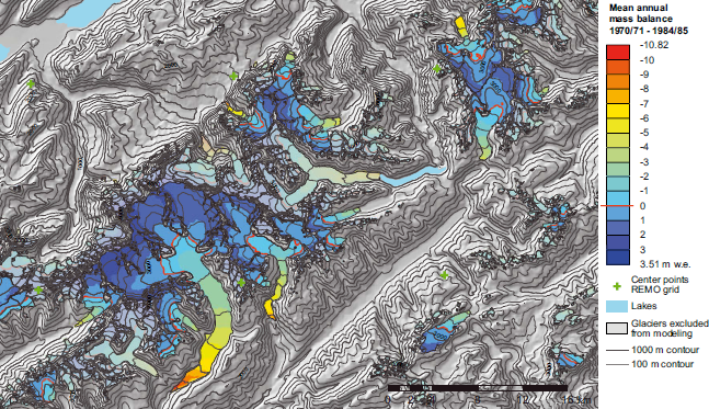
Modeled mean annual mass-balance distribution for the Aletsch region is shown in Figure 4. Mean modeled annual mass-balance profiles from a selection of 18 glaciers are displayed in Figure 5. On several glaciers (e.g. Findel, Festi, Fiescher) mass balance decreases almost linearly below the ELA while other glaciers show a more discontinuous decrease (e.g. Oberer Grindelwald, Saleina, Plaine Morte). Aletsch, Gorner and Oberer Grindelwald even show a pronounced increase in mass balance near the tongue, due to reduced radiation at the glacier tongues, as discussed in more detail in Section 6. Mass-balance profiles in the accumulation area are more similar, with a smaller gradient in accumulation towards higher elevations. The ELAs cover a considerable range of slightly less than 1 km, ranging from 2540 and 2570ma.s.l. (Blüemlisalp-Uri and Glarnischfirn, respectively) at the maritime northern edge of the Alps to 3450 and 3490 m a.s.l. (Weingarten and Hohbarg, respectively) in the dry interior parts of the Valaisan Alps. The large range in ELAs facilitates the following statistical parameter analysis.
Modeled mean annual mass-balance distribution (1970–85) for the region around Great Aletsch glacier. Mass-balance distribution for other glaciers than the selected 94 glaciers is shown with lighter colors. Background hillshading is derived from the swisstopo DEM also used for the modeling.
Mean modeled mass-balance profiles (1970–85) for 18
selected glaciers.

Interannual variability of mass-balance profiles is illustrated for Great Aletsch in Figure 6. The profiles are mostly parallel, with the exclusion of certain years (e.g. 1981). The difference between the most positive and most negative years is largest near the tongue and below the ELA and is smallest in the uppermost accumulation area.
Annual modeled mass-balance profiles for Great Aletsch glacier. The inverted mass-balance gradient at low elevations is in the model a result of strong shading on the narrow tongue located in a gorge.

Table 2 lists minimum, maximum and mean values as well as standard deviations of the 18 parameters and MP that have been derived from the DTM and the glacier polygons or from the modeled mass-balance distribution and the meteorological input fields. Note that all mass-balance parameters refer to a balanced-budget mass balance and the suffix 0 is omitted (e.g. AAR instead of AAR0) as explained in Section 2. The ELA is on average 23 m lower than zmid, but the standard deviation of the latter is somewhat larger. Mean ELA is overestimated by 60 m from zmed while the standard deviation is smaller. Average AAR is 0.59 with a standard deviation of 0.07. There is one remarkable outlier with an AAR of only 0.35 which is Plaine Morte, a large (9 km2) and flat plateau glacier with a weakly developed north-facing tongue. The low AAR is explained by the small mass-balance gradient over most of the ablation area (Fig. 5), resulting from a flat surface topography in the accumulation area with a smooth transition to the north-exposed ablation area. The continuously increasing slope towards the north leads to a reduction of solar radiation compensating for higher temperatures at decreasing elevations.
Mass-balance and topographic parameters and M P derived from mean annual mass-balance distribution and meteorological conditions; averaged over all 94 modeled glaciers and including the standard deviation (σ)

5.2. Correlation matrix
For all parameters listed in Table 2, the correlation coefficients (R) for linear fits x = β0 + β1y are displayed in a correlation matrix (Table 3). For most of the parameter correlations |R| ≥ 0.25, and the null hypothesis of parameters being uncorrelated can be rejected at the 0.01 level. However, statistical significance is considered to be of limited relevance here because the sample size is large and significance does not tell whether a relationship is sensible or can be transferred to reality. To make the correlation analysis comprehensible and verifiable, the regression coefficients β0 and β1 are listed in Table 4. Furthermore, a selection of six parameter pairs is depicted as scatter plots in Figure 7. For comparison to the model results, Figure 7b shows a number of glacier-specific observed relationships of T s ELA and P ELA available for the European Alps and Scandinavia (Reference Ohmura, Kasser and FunkOhmura and others, 1992).
Correlation matrix (R) for linear regression of mass balance and topographic parameters as well as M P of all 94 modeled glaciers.Correlation coefficients |R| ≥ 0.25 indicate a statistically significant correlation on the 0.01 level. Entries with |R| ≥ 0.58 (corresponds to R 2 ≥ 0.33) are in green; entries with |R| ≥ 0.81 (corresponds to R 2 ≥ 0.66) are in red

Regression coefficients for linear regression x = β 0 + β 1 y of mass balance and topographic parameters as well as MP of all 94 modeled glaciers. The coefficent β0 is given above the identity and β1 below identity. All coefficients are calculated with the parameter more to the left on the horizontal axis being the regressor (x) and the parameter more to the right being the dependent variable (y) (e.g. z med = 701.08 + 0.7760z mid)

Scatter plots for six selected parameter pairs. Because of its special characteristics, Plaine Morte (PM) is marked in all plots except (c) and (d): no H and Γacc was calculated for Plaine Morte because its accumulation area spans less than five elevation bands. Dotted lines indicate regressions excluding Plaine Morte. Marmolata glacier (M) is marked in (b).

The correlation values provide a first general characterization of the dependencies among the investigated parameters. Of course, many of them are intrinsically clear or long known and do not require detailed explanation: Highest correlations are found between ELA and z med (Fig. 7a) and b t and Δz, followed by ELA and z mid as well as P ELA and T s,ELA (Fig. 7b). The two meteorological variables P ELA and T s,ELA are closely related because ablation is an increasing function of air temperature, accumulation is an increasing function of P and by definition ablation equals accumulation at the ELA. Interestingly, regressing AccELA to T ELA and T s ELA yields lower correlations than regressing P ELA to the two aforementioned parameters. While certain correlations are lower than expected (e.g. Γabl, Γacc and H show generally intermediate or low correlations; cf. Fig. 7c and d), other correlations are unexpectedly high or even new: for example, Δz is highly correlated with b t (a correlation was expected but less pronounced) while the high correlation of AAR with b t or Δz are novel results (Fig. 7e and f). Furthermore z max and z min have opposite signs in their correlation with certain parameters and have intermediate or small correlations with any of the meteorological parameters, whereas z mid, z med and ELA are all highly correlated with them. Then b t has much lower correlations with the meteorological parameters than AAR, which is somewhat unexpected since b t is more directly related to meteorological conditions. While the mass-balance gradient in the accumulation region Γacc has intermediate correlation with P ELA or AccELA, Γabl does not show the often-mentioned correlations with T ELA and P ELA. The intermediate correlations of P ELA and AccELA with z max appear illogical at first sight, and explanations must be sought in the specific topography of the Swiss Alps rather than in the glacier-climate relationship. Finally S in,ELA and M p show only weak correlations with all other parameters. We attempt to explain expected but also unexpectedly high or low correlations in the following section and we hope that the results shown in the two matrices will encourage more detailed investigations in further studies.
6. Discussion
To determine how much the present modeling study is transferable to reality is challenging, because it is difficult to achieve realistic meteorological model input, and validation suffers from considerable uncertainty in observed mass balance and the small sample size of measured glaciers. Furthermore, the definitions of certain mass-balance parameters (e.g. b t, Γabl, Γacc) given in the literature (e.g. Reference CogleyCogley and others, 2011) are not detailed enough for the purpose of this study. Consequently it was necessary to develop methods for parameter retrieval as described in Section 4. Nevertheless a number of similarities but also a few differences were found between the synthetic glacier network and other data:
-
Modeled mass balance is close to the data from Reference Haeberli, Hoelzle and ZempWGMS (2007) and Huss and others (2010a,b), with both winter and summer balance being in a realistic range (Fig. 2). However, there is some disagreement between the two datasets used for validation that could be related to the different glacier samples and methods applied.
-
The balanced-budget AAR is 0.59, with a standard deviation of 0.07. On the one hand, an often used value is 0.67 for Alpine-type glaciers (Gross and others, 1976; Reference Braithwaite and MüllerBraithwaite and Müller, 1980). This value was derived from mass-balance observations on a small number of glaciers in the eastern Alps (Gross and others, 1976). On the other hand, Reference BahrBahr (1997) calculated a mean AAR for Alpine-type glaciers of 0.58 based on theoretical considerations. This value is supported by Reference Dyurgerov, Meier and BahrDyurgerov and others (2009), who derived a mean AAR of 0.58 from a worldwide sample of 86 series of mass-balance observations. The 13 Alpine series included have the same mean AAR and a standard deviation of 0.09.
-
The mean modeled ELA is very similar to mid-range and median glacier elevation (Table 2). The same is true when mid-range and median glacier elevation are compared to observed ELAs on valley glaciers (Reference Braithwaite and RaperBraithwaite and Raper, 2009). Reference Cogley and McIntyreCogley and McIntyre (2003) also found a good agreement of mid-range glacier elevation with ELA.
-
The modeled annual mass-balance profiles (Fig. 6) show a maximum variability in the ablation area and a reduced variability in the accumulation area. This pattern agrees with observations on Alpine glaciers (Reference KuhnKuhn, 1984) and is also confirmed by the comparison of modeled and measured mass-balance profiles in Figure 3.
-
The observed five relationships of T s ELA and P ELA from the Alps (Reference Ohmura, Kasser and FunkOhmura and others, 1992) fit well into the relationship modeled here (Fig. 7b) and indicate a realistic glacier-climate relationship at the ELA. However the number of observations from the Alps is limited and they cover a much smaller range of T s,ELA and P ELA conditions than the model results. There is one clear outlier (Marmolata glacier) in the observations. Because this north-exposed glacier is flat and neither subject to strong shading nor fed by avalanches, we suspect that the observed Marmolata values are erroneous.
-
Notably, mean MP for all glaciers is 1.18 ± 0.38 (one std dev.), supporting the suggestion of Reference Schwarb, Daly, Frei and ScharSchwarb and others (2001) that their precipitation climatology for gauge undercatch in high-mountain terrain be corrected by a factor of 1.15-1.3.
The modeled Γabl (Table 2) seem low compared to previous studies (e.g. Aletsch glacier: modeled 0.76 m (100 m)-1; cf. 1.0 m (100 m)-1 according to measurements from 1950/51 and 1951/52 (Reference HaefeliHaefeli, 1962)). One reason is the small mass-balance gradients at the glacier tongues (Figs 5 and 3a). Reduced mass-balance gradients are observed in reality (see Reference OerlemansOerlemans, 2001, for a selection of observed mass-balance profiles), but are usually less pronounced than in the model, where strong shading on glacier tongues located in gorges is considered realistically, while the important effect of enhanced longwave radiation from the rock walls is neglected (cf. Reference Machguth, Paul, Kotlarski and HoelzleMachguth and others, 2009). On the one hand, the possibly underestimated Γabl might be one reason that this parameter does not show a higher correlation with other parameters. On the other hand, an overestimation of bt would be the main reason for the low Γabl but bt shows all the expected correlations. Furthermore, mean B s and B a are both slightly underestimated (Table 1). In the comparison the glacier samples are different and both datasets (this study and Reference Huss, Hock, Bauder and FunkHuss and others, 2010a, Reference Huss, Usselmann, Farinotti and Bauderb) rely, although to a differing degree, on a mass-balance model. Nevertheless, this could indicate that modeled mass-balance gradients and hence also mass turnover are somewhat too low.
6.1. Analysis of parameter correlations
A high correlation of b t with AAR was found (Fig. 7f). The reason is related to the influence of glacier-specific hypsometry on AAR (Reference Furbish and AndrewsFurbish and Andrews, 1984): glaciers with long, narrow tongues reach further down and require a higher AAR to balance larger mean melt over their ablation area. A correlation between the hypsometry index and AAR was indeed observed (Fig. 7d) but is not strong. The two most remarkable outliers, with H > 4, are upper Grindelwald glacier (H = 6.7) and Glacier du Trient (H = 4.9). In both cases the ELA separates a gently sloping and wide accumulation area from a narrow and very steep tongue. H is calculated in a simple way where the effect of surface slope on the area per elevation interval is neglected. It remains to be tested if a more comprehensive description of hypsometry would result in a higher correlation with AAR. For instance, using modeled ELA instead of zmed to calculate H results in a higher R 2 (0.39) for the correlation with AAR but the H thus derived depends on prior knowledge of mass-balance distribution and cannot easily be applied to unmeasured glaciers.
The rationale behind Δz and bt being better correlated than bt and z min is that Δz = 2(z mid - z min) and Γabl Δz/2 ≈ b t because zmid is a good indicator of ELA (e.g. Reference Haeberli and HoelzleHaeberli and Hoelzle, 1995; Reference Braithwaite and RaperBraithwaite and Raper, 2009) and Γabl does not vary strongly among the different glaciers (Table 2). In other words Δz is a good measure of the vertical distance between ELA and the tongue. Reference Haeberli and HoelzleHaeberli and Hoelzle (1995) assessed melt at the tongue according to b t = Γabl(z mid - z min), and from analyzing observational data Reference Dyurgerov and BahrDyurgerov and Bahr (1999) concluded that z mid - z min is better correlated to b t than z min. The reason that z min is less indicative is that the balance rate at a given elevation varies strongly from more maritime to more continental glaciers.
A novel result is the quite strong positive correlation between Δz and AAR (Fig. 7e). One possible reason for this lies in the, albeit weak, negative correlation of Γacc to Δz: A lower Γacc means that the glacier tends to have a smaller mean accumulation (calculated over the accumulation area) and thus requires a larger accumulation area to balance melt in the ablation area (cf. Reference Furbish and AndrewsFurbish and Andrews, 1984). The linear fit of Δz to AAR provides a 0.5 AAR value for elevation ranges decreasing towards zero (very small glaciers or flat ice caps without outlet glaciers), while values around 0.7 seem to be characteristic of the (largest valley) glaciers with elevation ranges of 1500 m and more. The scatter of about ±0.05 for a given extent in altitude is considerable and most probably related to the hypsographic conditions of individual glaciers. The reasons behind the still remarkable general trend are worth exploring in more detail.
Other interesting relationships are those between Γacc and maximum elevation and Γacc and precipitation/accumulation (Fig. 7c). On a global scale, Γabl is considered dependent on the precipitation regime (e.g. Reference OerlemansOerlemans, 2005). In the Swiss Alps, where the range in Γabl and P is much smaller than globally, no correlation between Γabl and PELA was found. This is attributed to the dominance of small-scale effects (cf. Reference Oerlemans and HoogendoornOerlemans and Hoogendorn, 1989). However, in the accumulation area the expected increase in r with increasing precipitation/accumulation at the ELA (cf. Reference KuhnKuhn, 1981; Reference OerlemansOerlemans, 2001) was found. In the model simulation, the decrease in Γacc with increasing maximum altitude primarily reflects the nonlinear lowering of the sum of positive temperatures. In reality it could also reflect the well-known decrease in precipitation with colder and less humid air temperatures and stronger winds, more easily eroding the drier snow at higher altitudes (cf., for the Alps, Reference Haeberli and AleanHaeberli and Alean, 1985).
The two parameters correlating least with other parameters are MP (see Section 6.2) and S in ELA. The latter shows only a weak negative correlation with T ELA and T s,ELA. The two correlation pairs indicate that glaciers that receive more global radiation (e.g. south-facing glaciers) need lower air temperatures at the ELA (e.g. higher ELAs).
Finally, it must be noted that correlations do not necessarily result from processes in the glacier-climate system (here represented by the mass-balance model), but can also be related to the chosen glacier sample or simply the characteristics of glacier distribution in a certain area. For instance, a negative correlation of zmax with PELA is observed (Table 3) which indicates that glaciers at higher elevations are located in drier areas. This is indeed the case in the Swiss Alps, where most of the highest peaks are located in the comparably dry Valais region. Hence, the findings of this study should be applied to other regions only tentatively, as shown by the strong relationship found between Ts ELA and PELA: Observations from the Alps confirm the model results, but the relationship looks different for Scandinavian glaciers (Fig. 7b). Differences among regions are related to differing climate regimes that determine weights of the components of the energy balance.
6.2. Influence of the precipitation correction on mass-balance parameters
To achieve Σ B a ≈ 0 m w.e., precipitation is multiplied with a glacier-specific factor MP . The correction factor is uniform over each glacier's surface, so MP < 1 will lead to a reduction of the precipitation gradient γ P and values of MP > 1 will increase γ P . The precipitation gradient influences the modeled mass-balance distribution, so there is a potential feedback of the precipitation correction onto mass-balance parameters that needs to be evaluated.
Glacier-specific MP are correlated to all glacier parameters using linear regression (Table 3). Among the mass-balance parameters a weak correlation was found with AAR and Γacc (R2 ≈ 0.16) and a moderate negative correlation with P ELA, T ELA and AccELA (R2 ≈ 0.28). The latter correlations are to be expected, because MP < 1 always raises the ELA towards colder and drier conditions and vice versa. Furthermore, all parameters that indicate glacier elevation (ELA, z med, z mid, z max) show a weak negative correlation with MP (R2≈ 0.15-0.18). There are two possible reasons for this: (1) The mass-balance model could tend to overestimate mass balance at high altitudes, which must be corrected by reducing precipitation through M P. A possible explanation is the erosion of snow by wind that is not included in the model. On the other hand, the model also excludes refreezing processes which actually enhance accumulation at very high elevations in the Alps. (2) The precipitation climatology from Reference Schwarb, Daly, Frei and ScharSchwarb and others (2001) overestimates precipitation at high altitudes, and a correction is actually needed. There are almost no reliable precipitation observations above 2700ma.s.l. (Reference SevrukSevruk, 1997) that could reduce uncertainties in the PRISM (Parameter elevation Regressions on Independent Slopes Model) interpolation (Reference Daly, Neilson and PhillipsDaly and others, 1994) applied by Reference Schwarb, Daly, Frei and ScharSchwarb and others (2001). Although weak, the dependency of Mp and parameters related to glacier elevation needs further investigation. We conclude that the influence of the precipitation correction on mass-balance parameters is small and has a limited influence on the results of the correlation analysis.
6.3. Implications of the results
In regard to possible applications of geometric inventory data for estimating important glacier and climate variables, relations between information about glacier elevation and ELA, AAR, Γ, b t and accumulation or precipitation at the ELA are of great interest. The present study again confirms the close correlation between mid-range glacier elevation and ELA for a zero mass balance as already derived from field measurements (Reference Braithwaite and MüllerBraithwaite and Muller, 1980; Reference Braithwaite and RaperBraithwaite and Raper, 2009) and applied to a large numbers of glaciers in entire mountain chains by Reference Haeberli and HoelzleHaeberli and Hoelzle (1995) and Reference Hoelzle, Chinn, Stumm, Paul and HaeberliHoelzle and others (2007). Using mid-range elevation instead of median elevation where hypsographic information is unavailable, introduces a rather small quality reduction in the relation for valley-type glaciers. This important result definitively opens the way for easily estimating balanced-budget ELA values from modern glacier inventory data at regional to continental and even global scales. It also provides a simple and transparent rule of thumb for estimating long-term climate-change impacts on glaciers for everybody, including non-academics: half the change in minimum elevation since the end of the Little Ice Age quantitatively reflects the corresponding rise in ELA since that time or - looking into future scenarios - lower glacier margins will rise to higher elevations by about twice the shift in ELA for a given climate scenario (e.g. a 300 m ELA shift roughly corresponding to a 2°C warming would force the lower glacier margin to rise by ~600 m). The importance of such robust and transparent rules of thumb should not be underestimated: they are most efficient tools for enhancing public awareness of realistic glacier scenarios in a warming world and help avoid grave misunderstandings. They can also serve as plausibility checks in comparison with more complex model approximations, which add information about the timescales involved.
Besides median and mid-range elevation, the vertical glacier extent has a strong predictive potential with respect to important glacier characteristics (cf. Reference Haeberli and HoelzleHaeberli and Hoelzle, 1995; Reference Dyurgerov and BahrDyurgerov and Bahr, 1999; Reference Hoelzle, Chinn, Stumm, Paul and HaeberliHoelzle and others, 2007). Its close relation to the balance b t at the lower glacier margin enables corresponding estimates for unmeasured glaciers without the need to derive them from a distributed mass-balance model for each glacier. Knowledge of typical Γ values from a few glaciers would be sufficient to determine b t for all of them. In combination with ice thickness estimates from the same vertical extent and overall slope (e.g. Reference Haeberli and HoelzleHaeberli and Hoelzle, 1995; Paul and Linsbauer, in press), this allows dynamic response times to be estimated. Over time intervals corresponding to such dynamic response times, the mean mass balance can be estimated from the cumulative length change and the total length of a glacier, or, with a view to the future, the length change of a glacier for a given mass-balance scenario (Reference Haeberli and HoelzleHaeberli and Hoelzle, 1995). It must be kept in mind, however, that b t is indeed calculated from elevation information, directly depends on the mass-balance gradient and in the real world can be strongly influenced by effects such as albedo changes, debris cover, proglacial lake formation, subglacial ablation or collapse phenomena (Reference PaulPaul and others, 2007). The uncertainty of values estimated for unmeasured glaciers could therefore be considerable.
Fundamentally important relations for practical applications with glacier inventory data are those between air temperature and accumulation/precipitation at the equilibrium line. As first recognized decades ago (Reference AhlmannAhlmann, 1924; Reference Kotlyakov and KrenkeKotlyakov and Krenke, 1982; Reference Ohmura, Kasser and FunkOhmura and others, 1992), such relations open the possibility of treating large samples of inventoried glaciers as some sort of 'natural precipitation gauges', i.e. estimating regional patterns of precipitation distribution and making realistic approximations of absolute precipitation in high-mountain regions, where direct measurements are difficult, highly uncertain and in most cases simply non-existent. Because of the strong (auto)correlation between summer and annual mean air temperature, the quality loss from substituting the mean annual temperature for the physically more plausible summer temperature remains small. This, in turn, opens other important perspectives, as mean annual air temperature can be related to englacial temperature conditions (Reference Hooke, Gould and BrzozowskiHooke and others, 1983) and to thermal conditions, especially permafrost, in the surrounding areas.
7. Conclusions and Outlook
In this study, we have explored new ways of analyzing output from glacier mass-balance models. We have shown that modeling large glacier samples results in a reasonable mass-balance distribution and glacier parameters derived there from generally agree with the observations. The relationship of 18 glaciological and topographical parameters (and Mp) from 94 glaciers was analyzed in a correlation matrix, revealing dependencies between parameters that were already known from observational data, but also dependencies previously not described (e.g. AAR and b t, AAR and Δz). The latter deserve further analysis in future work and show the advantage of improved statistics owing to the possibility of modeling a much larger number of glaciers than are measured.
Emphasis was given to choosing a realistic model scenario and to bias correction of the input data. Nevertheless, transferring model results to reality is a critical issue in the approach. Validation is hampered by a lack of observational data and considerable uncertainties therein. The latter also originate from imprecise or missing definitions of mass-balance parameters. However, in contrast to the heterogeneous observational data, the uniform nature of a mass-balance model bears a danger of systematic offset and biases in the output. Although model and observations are mostly consistent, it was shown that in its current version the model tends to underestimate melt at the glacier tongues and there is evidence for too small mass-balance gradients. These points need to be improved in future work.
It was the aim of this study to analyze glacier mass-balance model output in terms of a synthetic mass-balance network and to evaluate its potential to complement observational datasets. In view of the promising results, the approach certainly deserves further attention. Future improvements of the methodology should be made with the mass-balance parameter's field of application in mind. A task specific to mass-balance parameters and equally important to synthetic and observational data will be to comprehensively define important parameters such as the balance rate at the tongue or the mass-balance gradients. Of general importance are improvements to models and input parameters. There is a current trend towards applying glacier mass-balance models to larger glacier samples using different mass-balance models and developing approaches to optimize input data (e.g. Jarosch and others, 2010). Our approach will likely benefit from these efforts. It is envisaged that results of different mass-balance models will be considered and the parameters analysed here will also be investigated in climatologically differing regions and for different glacier geometries (e.g. ice caps). The latter is important because studies working with glacier parameters usually cover extended spatial and temporal domains (e.g. Reference Kerschner, Kaser and SailerKerschner and others, 2000; Reference Hoelzle, Chinn, Stumm, Paul and HaeberliHoelzle and others, 2007). The lack of observational data will be a permanent issue requiring considerable efforts to be made to maintain a solid link between observations and the model world. This connection is fundamental to the quality of parameters derived from the synthetic networks and highlights the importance of observational data series.
Acknowledgements
We acknowledge MeteoSwiss for providing the meteorological observations, and swisstopo for the DTM. We thank the Max Planck Institute for Meteorology, Hamburg, Germany, for making the REMO output available to us. The detailed and constructive recommendations of two anonymous reviewers are gratefully acknowledged. This work was funded by the ice2sea program of the European Union 7th Framework Programme, grant No. 226375. This is ice2sea contribution No. 065.
Appendix: De-Biasing of The RCM Data
In this study, entire arrays of RCM output are de-biased and both the spatial (e.g. a wrong precipitation pattern) and the temporal dimension (e.g. a cold-winter bias in T) of biases have to be analyzed. Different approaches of bias correction are applied for T, S in and P, depending on the availability of datasets suitable to establish bias characteristics. The data used to analyze biases in T and Sin are meteorological observations from the 14 high-mountain weather stations (Fig. 1), and for P the precipitation climatology from Reference Schwarb, Daly, Frei and ScharSchwarb and others (2001) is utilized. While the latter covers 1971-90 and thus mostly includes the time-span of the model run (1970-85), the time frame of the observational data of T and S in refers to the 1981-2003 period. Prior to 1981 there were fewer high-mountain stations measuring T and very few measuring S in. We decided that it is more reasonable to establish the RCM bias from a larger number of observations and assume that the bias is also valid for the period of the model run, than to work with the very limited number of observations available before 1981.
To determine biases in T and S in we compare the measured values at the weather stations to the modeled values of their corresponding gridcells. Note that 'modeled' refers to the data as applied for the mass-balance computation, i.e. REMO data that have already been downscaled and interpolated to the DTM resolution as described in the main part of this paper. The comparison is performed at a daily temporal resolution over the time-span 1981-2003, and the mean modeled and the mean measured values at each station are computed for each day of the year (day No. 1-366). In Figure 8, modeled and measured cycles of mean annual air temperatures (Fig. 8a) and global radiation are shown (Fig. 8b). The temporal dimension of the biases is assessed by comparing modeled and measured mean annual cycles. A rough estimate of the spatial variability of biases is derived from the station-specific mean deviations between measured and modeled T as well as S in; both are shown in Figure 8.
Comparison of RCM (not bias-corrected) and measured annual curves of air temperature and global radiation, averaged over 1981–2003. The bold lines depict the mean modeled and measured curves for all stations. The thin lines depict the differences (downscaled RCM– measured) at the individual stations. Dotted thin lines indicate stations located below 2000ma.s.l. All curves, except for ‘S in clear sky’ are smoothed with a 15 day running mean for better readability.

The bias in T varies strongly with time, whereas, at least during summer, spatial variability is already simulated satisfactorily from REMO and the chosen lapse rate (cf. Reference KotlarskiKotlarski, 2007; Reference Kotlarski, Paul and JacobKotlarski and others, 2010). RCMs have difficulty in correctly reproducing the annual cycle of T over complex Alpine terrain (Suklitsch and others, 2010), and REMO shows a cold bias in winter independent of the difference in RCM gridcell and weather-station elevation (Reference Kotlarski, Paul and JacobKotlarski and others, 2010). Consequently, it was decided to perform a temporal correction of T by calculating the difference between mean measured and modeled T for every day of the year. The calculated daily offset in T is then added uniformly to the entire input arrays of air temperature depending on the day of the year. Spatial variability of biases in T is not corrected because it is most pronounced during winter when accuracy is less important for Alpine glacier mass balance. Furthermore Figure 8 also shows that the bias at all stations above 2000 m a.s.l. is rather similar.
Conversely, S in would require both a spatial and a temporal bias correction as indicated by the general overestimation during summer and the large variability of biases at the individual stations (Fig. 8b). Although biases are generally large, it must be stated that the weather stations with the most pronounced errors (Pilatus, S?ntis, Grimsel, Grand St Bernard, Moleson) are either located at the northern edge of the Alps where almost no glaciers exist or they are located on passes where local clouds tend to form frequently. By contrast, stations located in the more interior parts of the Alps on summit-like locations (Jungfraujoch, Corvatsch, Gütsch) are assumed to be more representative of the glacierized areas and have less pronounced biases. Correcting the spatial variability is also desirable, but difficult because the number of available stations is too small to derive the assumed rather complex bias pattern and to define the parameters controlling the pattern. The errors in the calculated global radiation stem mainly from erroneous cloudiness values obtained from the RCM (n RCM). During summer, RCM cloudiness is far too low, due to the parameterization of convective clouds implemented in REMO (cf. Reference Machguth, Paul, Kotlarski and HoelzleMachguth and others, 2009). Consequently, biases in S in are corrected by adjusting n. However, cloud observations (n meas) are not carried out at the 14 automatic synoptic weather stations, so nmeas is calculated from measured Sin and the calculated potential clear-sky radiation by solving the relationship from Reference Greuell, Knap and SmeetsGreuell and others (1997) (Section 4.1) for n.
Values for cloudiness range from 0 (no clouds) to 1 (completely overcast), and a bias correction must not result in any values exceeding these thresholds. Furthermore, the percentage of days with cloud-free or completely overcast conditions should match the observations. We apply cumulative distribution functions (CDFs) matching on a monthly basis to adjust n RCM to n meas. A total of 12 monthly CDFs of nRCM and 12 monthly CDFs of nmeas are calculated from all daily values of nRCM or nmeas at the 14 weather stations that fall into each month. Two examples of calculated CDFs, for March and August, are presented in Figure 9. These two months have been chosen because in March the RCM overestimates n meas the most, whereas in August the underestimation is most pronounced (see also Fig. 8b). Monthly transfer functions are then calculated to match the CDF of n RCM to the CDF of n meas. During the actual model run, each gridcell value of each daily grid of interpolated RCM cloudiness is then shifted by applying the transformation function of the respective month.
The effect of de-biasing through CDF matching on modeled cloudiness for March and August. The CDF of RCM cloudiness before and after de-biasing are shown together with the CDF of measured n (derived from measured and potential S in).

The applied bias corrections result in a much better agreement of measured and modeled values of air temperatures (not shown) and global radiation (Fig. 10). The curve of modeled Sin now fits well to the observed annual cycle. The bias of Sin during summer was reduced from nearly 60 Wm-2 to ~5 Wm-2. The remaining small bias is due to an overestimation of clear-sky days (cloudiness = 0) in the RCM during summer. These events cannot be directly corrected through CDF matching because the allocation to values of n meas is non-unique. To correct them as well would require additional information to be used (e.g. P) in the CDF matching.
Bias correction and subgrid parameterization of P are performed in one step, utilizing the precipitation climatology from Reference Schwarb, Daly, Frei and ScharSchwarb and others (2001). The dataset provides mean precipitation distribution for the greater Alpine area over the 1971-90 time-span at 2.5' (~2 km) spatial resolution. In this study a spatial correction array (P scale) for the glaciated areas is calculated from the ratio of mean annual P (1971-90) according to REMO and mean annual P (1971-90) according to Reference Schwarb, Daly, Frei and ScharSchwarb and others (2001). Before the calculation of P scale, both datasets were resampled to 100m cell size: Reference Schwarb, Daly, Frei and ScharSchwarb and others (2001) by bilinear interpolation and REMO by TPS. The resulting Pscale has a maximum of 2.6 and a minimum of 0.42. The mean value is 1.33 and reflects the fact that glacier areas on the DEM are on average situated at higher elevations than the coarse gridcells of the RCM. Very high and very low values of P scale can stem from bias in the RCM data but also from large local differences in topography between the high-resolution DEM and the coarse RCM. The correction array is then applied to all daily precipitation arrays from REMO which were also interpolated to a 100 m grid before. This methodology guarantees that the long-term mean precipitation agrees with Reference Schwarb, Daly, Frei and ScharSchwarb and others (2001) while daily variability is acquired from REMO. The same principle of spatio-temporal decomposition was applied by Reference Paul and KotlarskiPaul and Kotlarski (2010). As the Reference Schwarb, Daly, Frei and ScharSchwarb and others (2001) dataset is based on uncorrected precipitation measurements, precipitation is somewhat too low and we expect that mean modeled mass balances are below measured ones. The precipitation correction factor MP is introduced to correct for this general bias, for the more pronounced local over- and underestimations of high-mountain precipitation in the Reference Schwarb, Daly, Frei and ScharSchwarb and others (2001) dataset as well as for preferential accumulation of snow on the glacier surfaces (see Section 4.3).
Effect of the performed bias correction for global radiation. The uncorrected and the bias-corrected mean curves of modeled S in for all 14 stations are shown and can be compared to the mean measured annual cycle of S in. All curves are smoothed with a 15 day running mean for better readability.


