

1. Introduction
Ice shelves are the floating extensions of the large polar ice sheets and are predominantly found around Antarctica. Re cent discussion of the rate of global sea-level rise emphasizes the crucial role of ice shelves at the conjunction between atmosphere, ocean and large ice sheets. A shrinkage, or even a loss, of buttressing ice shelves has only a relatively small direct effect on this sea-level rise (Reference Jenkins and HollandJenkins and Holland, 2007; Reference Shepherd, Wingham, Wallis, Giles, Laxon and SundalShepherd and others, 2010), but it can cause an acceleration and thinning of the upstream tributaries, which increases solid ice discharge from the ice sheet (Reference Rott, Rack, Skvarca and DeRott and others, 2002, Reference Rott, Muller, Nagler and Floricioiu2007, Reference Rott, Muller, Nagler and Floricioiu2011; Reference De Angelis and SkvarcaDe Angelis and Skvarca, 2003; Reference Joughin, Abdalati and FahnestockJoughin and others, 2004; Reference Rignot, Casassa, Gogineni, Krabill, Rivera and ThomasRignot and others, 2004, Reference Rignot2008; Reference Scambos, Bohlander, Shuman and SkvarcaScambos and others, 2004; Reference Cook, Fox, Vaughan and FerrignoCook and others, 2005; Reference RignotRignot, 2006; Reference Bamber, Alley and JoughinBamber and others, 2007; Reference GudmundssonGudmundsson, 2007; Reference Shepherd and WinghamShepherd and Wingham, 2007; Reference Glasser and ScambosGlasser and Scambos, 2008; Reference Cook and VaughanCook and Vaughan, 2010, Reference Joughin and AlleyJoughin and Alley, 2011). Numerical studies are, in principle, able to reproduce this behavior (Reference Schmeltz, Rignot, Dupont and MacAyealSchmeltz and others, 2002; Reference Payne, Vieli, Shepherd, Wingham and RignotPayne and others, 2004; Reference Thomas, Rignot, Kanagaratnam, Krabill and CasassaThomas and others, 2004).
Gravitational driving stresses in ice shelves must be balanced by drag at the lateral shelf margins due to the lack of basal traction. Fractures affect this stress balance by disturbing the ice body’s mechanical integrity (e.g. Reference Larour, Rignot and AubryLarour and others, 2004a, Reference Larour, Rignot and Aubryb; Reference Vieli, Payne, Du and ShepherdVieli and others, 2006, Reference Vieli, Payne, Shepherd and Du2007; Reference Khazendar, Rignot and LarourKhazendar and others, 2009; Reference Humbert and SteinhageHumbert and Steinhage, 2011) and thereby reducing the buttressing effect (Reference Dupont and AlleyDupont and Alley, 2005; Reference Gagliardini, Durand, Zwinger, Hindmarsh and Le MeurGagliardini and others, 2010). Hence, prognostic ice-sheet models need to incorporate at least the large-scale effects of the complex physics of fracture processes.
Fractures develop from small-scale flaws that have sufficient initial size (Reference Rist, Sammonds, Murrell, Meredith, Oerter and DoakeRist and others, 1996, Reference Rist1999), most likely initiated close to the surface, where the compressive overburden stresses are small. They form in the presence of strong divergence or convergence of the ice flow (Reference HughesHughes, 1977, Reference Hughes1983) or due to the buckling and shearing close to ice rises and side margins (e.g. Reference GlasserGlasser and others, 2009; Reference Cuffey and PatersonCuffey and Paterson, 2010). Also, the abrupt acceleration and cyclic tidal flexure (e.g. Reference HoldsworthHoldsworth, 1977; Reference Lingle, Hughes and KollmeyerLingle and others, 1981) in the transition zones between grounded or stagnant parts and fast-flowing units of floating ice shelves support fracture formation. As a basic approach, the initiation and growth of large-scale fractures close to the surface, so-called surface crevasses, can be considered in terms of horizontal strain rates or surface stresses. This is a simplification, since, in gen eral, brittle fracture formation is known to depend on the total stress tensor across a crack (Reference LawnLawn, 1993; Reference Paterson and WongPaterson and Wong, 2005). The presence of water strongly influences fracture growth. At the bottom of the ice shelf, crevasses can extend far upward into the ice body, due to sea-water penetration (Reference WeertmanWeertman, 1980; Reference Jezek and BentleyJezek and Bentley, 1983; Reference Van der VeenVan der Veen, 1998a; Reference Rist, Sammonds, Oerter and DoakeRist and others, 2002; Reference Luckman, Jansen, Kulessa, King, Sammonds and BennLuckman and others, 2011). At the surface, meltwater-enhanced fracturing has been pro posed as one of the triggers of the catastrophic disintegration of several ice shelves fringing the Antarctic Peninsula in re cent decades (Reference WeertmanWeertman, 1973; Reference Doake and VaughanDoake and Vaughan, 1991; Reference Rott, Skvarca and NaglerRott and others, 1996; Reference Scambos, Hulbe, Fahnestock and BohlanderScambos and others, 2000, Reference Scambos, Bohlander, Shuman and Skvarca2009; Reference MacAyeal, Scambos, Hulbe and FahnestockMacAyeal and others, 2003; Reference Rack and RottRack and Rott, 2004; Reference Khazendar, Rignot and LarourKhazendar and others, 2007; Reference Van der VeenVan der Veen, 2007; Reference Vieli, Payne, Shepherd and DuVieli and others, 2007; Reference Glasser and ScambosGlasser and Scambos, 2008; Reference Braun, Humbert and MollBraun and others, 2009).
Considerable effort has been made to incorporate fracture mechanics into regional diagnostic ice-shelf models: Reference RistRist and others (1999), Reference Hulbe, Ledoux and CruikshankHulbe and others (2010) and Reference Jansen, Kulessa, Sammonds, Luckman, King and GlasserJansen and others (2010) use a mechanistic two-dimensional (2-D) fracture criterion in diagnostic models to evaluate the stability of the Filchner-Ronne and Larsen C ice shelves, respectively. Reference Humbert, Kleiner, Mohrholz, Oelke, Greve and LangeHumbert and others (2009) identified shear zones and rifts in the Brunt Ice Shelf using observational data and applied additional flow-enhancement factors and a decoupling schemeforthe stress balance. Reference Saheicha, Sandhäger and LangeSaheicha and others (2006) use the von Mises criterion (Reference VaughanVaughan, 1993), which expresses a relationship between tensile strength and effective stress. The macroscopic effect of fracture structures on the ice body of the Filchner-Ronne Ice Shelf (FRIS) in the diagnostic model is parameterized by softening and decoupling, in order to reproduce characteristic features of the observed velocity distribution. These models identify regions of potential crack opening for given boundary conditions and evaluate their effects on the stress balance. Sandhager and others (2005) additionally introduced the advection of a variable with the diagnostic velocity field accounting for a shear-zone depth ratio healed with a constant rate.
In order to represent the manifold physical role of fractures on large-scale ice-sheet dynamics we need a well-defined time-evolving field, which is advected with the ice flow. Here we introduce this field as a measure for fracture density and introduce first-order parameterizations for the relevant contributing processes, such as the initiation, growth or healing of fractures. The respective importance of these processes and parameters is evaluated in a suite of numerical experiments. Characteristics of fracture density along the flowline and in side shear regions are discussed for two idealized ice-shelf geometries. The individual pattern of fracture density for realistic scenarios, such as for the large FRIS or the smaller Larsen A+B ice shelf (LABIS) is compared with a snapshot of observed locations of surface features in these ice shelves.
2. Fracture-Density Field
We define a 2-D field, ?, over the entire ice-shelf region, which quantifies the mean area density of fractured ice. The unitless, scalar field variable, ?, is bounded by
where ϕ = 0 corresponds to non-fractured ice. In observed ice-shelf fracture fields the fracture density, ϕobs, is defined as the fraction of failed ice, i.e. ice that cannot be described appropriately by an ice-continuity condition (e.g. the Stokes equation). Thus, ϕobs increases with the number, N, and the length, l, of growing crevasses. Crevasses are discontinuities, which alter the local stress field within a zone of influence. For comparison with observational fields we assume that the area of failed ice around crevasses is rectangular, spanning a region of horizontal distance w around an individual crevasse. Groups of individual zones of influence can be quantified as a fraction of an ice-shelf surface section as

where Nw and l are limited to the extent of the discrete mesh, Δx and Δy. For ϕobs = 1 the zone of influence covers the entire discrete gridcell surface (e.g. Fig. 1b).
(a) Observed fracture density, ϕobs, in the Filchner–Ronne Ice Shelf based on data of Reference Hulbe, Ledoux and CruikshankHulbe and others (2010) and Eqn (2) with length-dependent width of the zone of influence, bounded by 1 km < w = l/4 < 10 km. Regions of vanishing fracture density are masked. Thin black and gray-dotted lines show the position of the grounding line and observed stream lines. (b) Close-up view of observed fracture density, ϕobs, overlaid by observed fractures (black) with associate zone of influence (gray contours). Main inlets and ice rises are denoted by abbreviations: R – Ronne Ice Shelf; F – Filchner Ice Shelf; EIS – Evans Ice Stream; CIS – Carlson Inlet; RIS – Rutford Ice Stream; IIS – Institute Ice Stream; MIS – M¨ oller Ice Stream; FIS – Foundation Ice Stream; SFIS – Support Force Ice Stream; REIS – Recovery Ice Stream; SIS – Slessor Ice Stream; FP – Foin Point; KIR – Korff Ice Rise; HIR – Henry Ice Rise; BIR – Berkner Ice Rise.

We consider here macroscopic structural glaciological fracture features, growing from the surface both vertically and horizontally, or closing in appropriate stress regimes. Although the vertical dimension of penetrating crevasses is an essential issue in the discussion of ice-shelf stability, it is not explicitly included in our definition. Instead we focus here on the location of surface crevasses, often collocated in band structures, revealing a depth-dependent density of crevasses. However, ϕ can be expanded to three dimensions, which will be the focus of future studies. In addition, here we do not take into account previous microscale stages of fracture formation, such as subcritical crack growth or damage accumulation (Reference WeissWeiss, 2004; Reference Pralong and FunkPralong and Funk, 2005). Such processes depend on the prevailing local stress and produce the flaws necessary to initiate crevasse opening, mostly in firn layers with distinct mechanical properties. Such flaws can hardly be detected at the ice-shelf surface, and do not contribute directly to the fracture density defined here. However, they do play an important indirect role for the fracture-density field, ?, by serving as starter cracks, from which the crevasses are initiated. In order to focus on the macroscopic dynamics of fracture growth, we assume a spatially homogeneous field of microcracks.
The fracture density, ϕ, is assumed to be isotropic and it is transported by horizontal advection with the vertically averaged velocity, v, calculated from the continuum mechanics stress balance in the shallow-shelf approximation (SSA) implemented in the Potsdam Parallel Ice Sheet Model, PISM- PIK (see Appendix for a brief description and Reference WinkelmannWinkelmann and others (2011) for further details) as
with forcing term f as the sum of sources, f
s, and healing terms, fh, which depend on a number of glaciological parameters. To leading order we assume here a sole dependence on the strain rate, ![]() , stress, σ, and the fracture density, ?, itself. For the source term we write
, stress, σ, and the fracture density, ?, itself. For the source term we write
where ψ is the fracture growth rate. The second factor reduces the source by (1 - ϕ) and represents the fracture interaction, bounding the resulting macroscopic fracture density below the threshold, 1. The justification for this term is that the local stress field surrounding a single crevasse is relaxed up to a distance of ~3-4 crevasse depths (Reference Sassolas, Pfeffer and AmadeiSassolas and others, 1996). For closely spaced crevasse bands and, hence, for a relatively high fracture density, additional fracture formation and further fracture penetration is hindered accordingly (Reference SmithSmith, 1976; Reference WeertmanWeertman, 1977).
2.1. Longitudinal spreading as source of fracture growth
Ice shelves spread under their own weight at a rate that is generally high in the vicinity of the grounding line, where it goes afloat. In two horizontal dimensions we attempt here a formulation using merely the eigenvalues of the vertically averaged strain-rate tensor, ![]() and
and ![]() , where
, where ![]() . These eigenvalues represent expansion
. These eigenvalues represent expansion ![]() or contraction
or contraction ![]() along the principal directions. In isotropic ice the initial opening of surface cracks is observed to be transverse to the principal direction of strongest stretching (Reference HoldsworthHoldsworth, 1969; Reference RistRist and others, 1999). For the purpose of this study, we use a simple formulation in terms of the maximum spreading rate (not the total effective strain rate) to capture the first-order effect and understand how much of the observed fracture fields can be reproduced by this simple approach. Hence, we formulate the fracture growth rate for the fracture-density source (Eqn (4)) as
along the principal directions. In isotropic ice the initial opening of surface cracks is observed to be transverse to the principal direction of strongest stretching (Reference HoldsworthHoldsworth, 1969; Reference RistRist and others, 1999). For the purpose of this study, we use a simple formulation in terms of the maximum spreading rate (not the total effective strain rate) to capture the first-order effect and understand how much of the observed fracture fields can be reproduced by this simple approach. Hence, we formulate the fracture growth rate for the fracture-density source (Eqn (4)) as
where γ is a unitless constant parameter which, in general, should be a function of flow law parameters, such as the temperature-dependent ice softness. For this uniaxial case without healing (fh = 0) we can derive, from Eqns (3-5), an exact analytical steady-state solution, which only depends on the velocity distribution, u(x), along the flowline,
and a given inflow velocity, u0 = u(x
0). The boundary value, ϕ0 = ϕ(x
0), is associated with pre-existing cracks which have formed upstream in the tributaries or with crevasses initiated at the grounding line (e.g. due to tidal flexure (Section 2.3)). In the unconfined flowline case, the function ϕ(x) is strictly monotonic, since ![]() is tensile everywhere, i.e. positive values meaning expansive flow. The parameter γ becomes an exponent here, determining the curvature of the function. The larger γ , the faster ϕ approaches saturation (at ϕ = 1).
is tensile everywhere, i.e. positive values meaning expansive flow. The parameter γ becomes an exponent here, determining the curvature of the function. The larger γ , the faster ϕ approaches saturation (at ϕ = 1).
Experiments with idealized ice-shelf geometry
In this first-order formulation we calculate the 2-D steady- state fracture density, ϕ(x, y), with PISM-PIK for an ice shelf confined in an idealized rectangular bay with unidirectional inflow (Fig. 2). We chose a parameter value γ = 0.5 for the fracture growth rate and boundary condition ϕ
0 = 0.1. The steady-state profiles of ice thickness, H, velocity, u, and hence the larger principal strain rate, ![]() , along the center line, x, of the wide ice shelf (Fig. 3a) are close to the analytical flowline solution of an unconfined ice shelf spreading in one direction (Reference Van der VeenVan der Veen, 1999; gray dashed curve in Fig. 3a and b) since in the wide geometry the buttressing effect of side drag is small in the inner part. Inserting this analytical velocity solution into Eqn (6) yields the fracture density
, along the center line, x, of the wide ice shelf (Fig. 3a) are close to the analytical flowline solution of an unconfined ice shelf spreading in one direction (Reference Van der VeenVan der Veen, 1999; gray dashed curve in Fig. 3a and b) since in the wide geometry the buttressing effect of side drag is small in the inner part. Inserting this analytical velocity solution into Eqn (6) yields the fracture density
where C = [ρg (ρw - ρ) /(4ρwB0)]3 = 2.45 × 10⁻¹⁸ m-3 s-1 comprises material constants, such as the ice density, ρ, sea water density, ρw, and the acceleration due to gravity, g, as well as the constant ice stiffness rate factor, B0. Even though in the simulations a temperature-dependent ice stiffness, B = B(T), is used, the obtained fracture density along the center line is very close to the analytical solution of Eqn (7) and increases up to a value of 0.4 at the mouth of the embayment. At the side margins, where friction is prescribed by a staggered boundary viscosity, strong shearing yields large magnitudes of both principal strain-rate components, while the minor component, ![]() , is generally compressive here with respect to the principal axes (Reference NyeNye, 1952). The parameterization presented here leads to steady-state values of the fracture density up to 0.8 close to the side margins (right column, Fig. 3a). Figure 3b shows the profiles of ice thickness and velocity of an ice shelf confined in a comparably narrow bay, 150 km wide and 250 km long. For the same lateral friction as for the wide-bay set-up we find a strong buttressing effect also in the inner part of the ice shelf, indicated by much thicker and slower ice compared to the less confined, i.e. wider, case. This leads to smaller spreading rates in the upstream region and hence to a smaller fracture density there. When the ice shelf leaves the narrow bay it can extend freely, which leads to maximal spreading rates, up to
, is generally compressive here with respect to the principal axes (Reference NyeNye, 1952). The parameterization presented here leads to steady-state values of the fracture density up to 0.8 close to the side margins (right column, Fig. 3a). Figure 3b shows the profiles of ice thickness and velocity of an ice shelf confined in a comparably narrow bay, 150 km wide and 250 km long. For the same lateral friction as for the wide-bay set-up we find a strong buttressing effect also in the inner part of the ice shelf, indicated by much thicker and slower ice compared to the less confined, i.e. wider, case. This leads to smaller spreading rates in the upstream region and hence to a smaller fracture density there. When the ice shelf leaves the narrow bay it can extend freely, which leads to maximal spreading rates, up to ![]() , and hence to a strong increase in fracture density close to the value of the wide ice shelf at this position. Accordingly, the profiles across the mouth of the narrow bay are similar to the results of the wide bay (compare right columns of Fig. 3a and b).
, and hence to a strong increase in fracture density close to the value of the wide ice shelf at this position. Accordingly, the profiles across the mouth of the narrow bay are similar to the results of the wide bay (compare right columns of Fig. 3a and b).
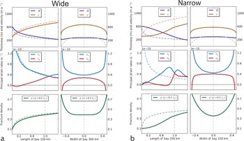
Steady-state fracture density, ϕ, for an ice shelf confined in a rectangular bay 300 km wide and 150 km long (left) or 150 km wide and 250 km long (right), with constant γ = 0.5. Ice flows into the bay at the top boundary with ϕ 0 = 0.1, ice thickness 600m and maximal speed 300ma−1. Along the sides, friction is parameterized by a viscosity ηB = 5×10¹³ Pa s. At the ice-shelf front, ice calves off for an ice thickness less than 175 m. Melting and accumulation is neglected. Black dashed lines show lateral and cross sections along which profiles are plotted in Figure 3.

Obtained velocity, ice thickness, principal horizontal strain rates and the inferred fracture-density field evolution for ice shelves confined in a rectangular bay (a) 300 km wide and 150 km long and (b) 150 km wide and 250 km long (Fig. 2). Profiles are normalized to unity length and width and plotted in lateral view along the center line (left panel columns) and across the mouth of the bay (right panel columns). The black dashed vertical line in the left panel columns shows the position of the mouth of the bay. The gray dashed profile on the upper right panel shows the unidirectional inflow velocity applied at the upstream boundary. Steady-state values in the wide case are close to the analytical solution of an unbuttressed flowline ice shelf plotted as dashed curve, whereas in the narrow case profiles vary strongly. In the lower panels steady-state fracture densities with ϕ0 = 0.1 are shown.
Experiments with a realistic ice-shelf geometry
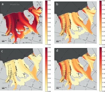
In a realistic set-up, such as for the FRIS, the resulting fracture-density field can be phenomenologically compared with observations, i.e. the location of areas with many surface features for a certain snapshot can be compared with features of the obtained fracture-density pattern, indicated by comparably high values. In contrast to the simulations with an idealized geometry (Fig. 2) we prescribe the ice thickness in the simulations with realistic topography and specify boundary conditions (see Section 2.2 and Appendix for precise values). This is necessary in order to avoid significant errors from a dynamic calculation of the flow field. We simulate the evolution of fracture density starting from an initial zero state in the whole ice-shelf domain. After reaching a steady state, fracture density is highest in the stagnant outer shear regions and downstream of regions that have been subject to shearing along the side margins or promontories (Fig. 4a). Separate flow units draining from different inlets can be identified in the structure, but the steady-state pattern of the fracture field appears comparably smooth. While the locations of some features compare well with observations, pronounced bands of observed surface features, as evaluated by Reference Hulbe, Ledoux and CruikshankHulbe and others (2010) from Moderate Resolution Imaging Spectroradiometer (MODIS) Mosaic of Antarctica (MOA) image maps, can hardly be identified in the fracture-density pattern. Fracture density is also high in areas where the flow is comparably slow, such as upstream of ice rises. Since, in reality, fractures are not expected to form in those low-strain-rate areas, this suggests the introduction of a critical threshold for fracture initiation. Observations suggest physically reasonable thresholds for crevasse initiation defined in terms of stresses, i.e. at high effective stresses (e.g. Reference VaughanVaughan, 1993). Below these thresholds fractures may close and heal due to the overburden pressure, accumulation or refreezing.
Steady-state distribution of the fracture density in a realistic set-up of the FRIS for varying fracture initiation thresholds, σcr: (a) 0 kPa, (b, d) 70kPa and (c) 90kPa in von Mises fracture criterion with fracture growth parameter γ = 0.3, and without contribution through the inlets, ϕ0 = 0. Results shown in (d) are obtained by choosing a fracture growth rate with a constant ![]() For a fixed ice thickness, a flow enhancement of Essa = 0.4 and with parameterized side friction by ηB = 1015 Pa s, the fracture density is transported with a steady SSA velocity field. Overlaid, observed visible surface fractures, kindly provided by Reference Hulbe, Ledoux and CruikshankHulbe and others (2010, Fig. 1).
For a fixed ice thickness, a flow enhancement of Essa = 0.4 and with parameterized side friction by ηB = 1015 Pa s, the fracture density is transported with a steady SSA velocity field. Overlaid, observed visible surface fractures, kindly provided by Reference Hulbe, Ledoux and CruikshankHulbe and others (2010, Fig. 1).
2.2. Crevasse initiation threshold
Observed crevasse bands downstream of inlet corners, converging streams and ice rises aligned in the flow direction suggest an initiation of fractures in the intense shearing regions once a certain threshold is reached. Based mainly on laboratory experiments, these critical values are often defined in terms of effective stress or similar rotational invariant flow properties, such as combinations of stress or strain-rate eigenvalues. Fracture initiation starts from the surface, where the overburden pressure vanishes. The mechanical properties of the upper firn layer are distinct, but strain rates are mostly constant with depth (Reference Nath and VaughanNath and Vaughan, 2003). A variety of phenomenological criteria, such as the von Mises criterion (Reference VaughanVaughan, 1993), the Coulomb criterion or even advanced mixed-mode crevassing with maximum circumferential stress criterion based on linear-elastic fracture mechanics (e.g. Reference Kenneally and HughesKenneally and Hughes, 2006), can identify regions where creep failure and fracture initiation most likely occur.
We choose the simple von Mises criterion, which is based on the so-called ‘maximum octahedral shear stress’, defined in terms of surface-parallel principal stresses, σ+ and σ -, as
The range of literature values of the tensile strength, σt, that ice can support is 90-320 kPa (Reference VaughanVaughan, 1993). This large range may be due to the uncertainty in stress/strain- rate conversion of observational data with the constitutive flow law, as well as to the effects of temperature, density and firn structure. Tensile strengths in Antarctic ice shelves are found around the median of this literature range. On the basis of the von Mises criterion we refine our fracture growth rate (Eqn (5)) to
where the additional ?(Δ) is the Heaviside step function to predict regions of potential fracture growth, defined as
In the following we discuss the effect of this critical value on the steady-state fracture-density pattern in a model of the FRIS. In order to be close to observed conditions, ice thickness and all other boundary conditions are prescribed and the three-dimensional (3-D) temperature evolution has already reached an equilibrium state close to observations. Some parameter must be determined to achieve the most realistic flow pattern for the given model configuration.
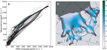
The lateral friction of the ice shelf, parameterized by the boundary viscosity, ηB, strongly influences the strain-rate and stress fields, and thereby the fracture-density field. Higher friction leads to vanishing ice speed along the margins and to strong shearing, but also to much slower speeds in the interior and outer parts of the ice shelf, which can be compensated by a larger enhancement factor. Comparison with reconstructed observational ice surface speed data (especially for lower speeds) suggests the use of a comparably small side friction (Fig. 5a). It was set to ηB = 1015Pas. This accounts for the partial decoupling of large interior flow units from the sides along weak zones. As long as this feature is not captured in the flow model (Section 3), a suitable enhancement factor for the SSA calculation has to be chosen. Such an enhancement factor is generally used to account for anisotropy and grain-size effects in the ice shelf (Reference Ma, Gagliardini, Ritz, Gillet-Chaulet, Durand and MontagnatMa and others, 2010). Hence, the vertically averaged effective viscosity in the SSA-stress balance scales with ESSA -1/n (Reference WinkelmannWinkelmann and others, 2011, their Eqn (10)). Best comparison with observations in the FRIS with a root- mean-square deviation of the velocity vector components of only 108 m a-1 averaged over ˜14 000 points and a cross correlation coefficient r2 = 0.96 is achieved with a relatively low value of EssA = 0.4.
(a) Scatter plot showing a comparison of calculated vs observed surface speed values within the ice-shelf domain for an optimal parameter configuration of ESSA = 0.4 and ηB = 1015 Pa s. (b) Distribution of calculated von Mises effective stress, σt, in the FRIS. Values larger than critical effective stress, σcr = 70 kPa, colored in purple, are found in confined shear regions at the inlets and some side margins and where flow units merge. A maximum spreading rate of ![]() is obtained in most parts of the indicated regions (thick brown contours). Thin brown contours delineate lower spreading rate, i.e. 1.5 and 2.0 × 10⁻¹⁰ s−1.
is obtained in most parts of the indicated regions (thick brown contours). Thin brown contours delineate lower spreading rate, i.e. 1.5 and 2.0 × 10⁻¹⁰ s−1.
The steady effective stresses inferred in this way are comparably low, and regions of likely creep failure identified with the von Mises criterion with a threshold below the literature range (e.g. σcr
= 70kPa) cover only 4% of the total FRIS area, indicated by purple shaded areas in Figure 5b. These shear regions are found at the major inlets, downstream of ice rises at flow unit junctions, but also at shearing margins, particularly in the narrow Filchner Ice Shelf. Thus, fractures grow according to the corresponding spreading rate, which is, on average, ![]() in those regions. In observations much higher strain rates are found in the confined suture zones and at shear margins. A softening of ice in areas of high fracture density would account for this effect (Section 3).
in those regions. In observations much higher strain rates are found in the confined suture zones and at shear margins. A softening of ice in areas of high fracture density would account for this effect (Section 3).
The modeled fracture-density value is associated with the frequency, length and width of the the zone of influence of fractures, but a precise quantitative validation can only be made on the basis of widespread ice-penetrating radar data. In our basic formulation we have to choose a somewhat arbitrary value for parameter γ , so the resultant fracture density produces a physically meaningful steady- state pattern, reflecting relevant features of observed surface structures (Fig. 4b-d). Maximum calculated fracture-density values peak around ϕ max = 0.8, particularly in the outer shear regions close to the front. In those regions the fracture interaction factor, (1 - ϕ), has a significant effect, which is expected in the dynamics of real crevasse trains.
For increasing fracture initiation threshold, σcr, we find more-pronounced band structures downstream of ice rises and prominent geographical features, which agrees with the location of crevasse trains in observations (compare Fig. 4a and b). For even higher threshold values (within the range of the literature values) some of the features are no longer reproduced (e.g. fractures in the suture zone of the merging flow units of Evans and Rutford Ice Streams (EIS and RIS) in Fig. 4c). Most relevant features of the observational data map are best represented for a threshold of σcr = 70kPa (Fig. 4b). The reddish bands (high fracture density) coincide very well with observed fracture bands and streak lines (except for those structures formed at ice rumples, that are not considered in our model, such as Kershaw ice rumples between FP and KIR). If we choose a length-dependent width, w = l/4 < 10 km, for the zone of influence around an observed crevasse, we can compute an observed fracture density snapshot, ϕobs on the 5 km grid (Eqn (2)). Figure 1 shows the resulting bands of high crevasse density aligned in the flow direction and in shear regions, which can be compared to the obtained smooth model fracture density, ϕ (e.g. Fig. 4). The close-up view in Figure 1 reveals the spatially varying distribution of ϕobs. A time average over several snapshots of sufficient delay would give a much smoother distribution. The width, w, scales the observed fracture density as long as the overlap of individual zones of influence is small. In any case, comparison of the model’s fracture field can only be complete if the area of failed ice can be determined from observations, since the geometrical derivation proposed here for surface crevasses is merely a rough approximation of the quantity that we proposed as the fracture field, ?. Large rifts observed close to the calving front are apparently not captured by the model ?. Since no healing is applied so far, the steady-state fracture density can also accumulate in very slow-moving sections, such as upstream of Berkner Ice Rise (BIR) supplied by the contributions of the Rutford and Foundation Ice Streams (RIS and FIS).
Regarding the effects of fracture initiation, ϕ(σt - σcr), and fracture growth rate, ![]() the resulting steady-state fracture-density pattern is apparently more sensitive to the fracture initiation threshold than to the growth rate. If we replace the spreading rate by its mean value found in the initiation regions, i.e.
the resulting steady-state fracture-density pattern is apparently more sensitive to the fracture initiation threshold than to the growth rate. If we replace the spreading rate by its mean value found in the initiation regions, i.e. ![]() , we get a similar pattern (compare Fig. 4b and d).
, we get a similar pattern (compare Fig. 4b and d).
Rist and others (1999, plate 1) provide a map of the FRIS crevasse pattern using visible and radar imagery. Most of the fracture features coincide with the map inferred by Reference Hulbe, Ledoux and CruikshankHulbe and others (2010), except for fracture fields in the central Ronne Ice Shelf downstream of Korff and Henry Ice Rises (KIR and HIR), probably ice with densely distributed short and inactive fractures covered with snow and not seen in visual inspection of MODIS images nor in the obtained fracture- density field.
In a simulation of the northern Larsen Ice Shelf (A+B) we use the same flow parameters as in the FRIS, which yields a velocity field that differs from observed velocities with a cross-correlation coefficient of r2 = 0.78. A varying combination of flow enhancement and friction parameter does not much improve this result. A fracture-density dependent rheology may correct for this underestimation of velocities, as in many other smaller buttressing ice shelves. Nevertheless, the evolution of the fracture density with parameters σcr = 70kPa and γ = 0.5 produces a pattern (Fig. 6) which compares well with the advanced satellite image interpretations of Glasser and Scambos (2008, Fig. 4). Elongated steady-state bands initiated at the inlet corners of the main tributaries following the ice flow down to the ice- shelf front agree with crevasse patterns in the images (at inlet corners even rifts are formed). Similar longitudinal structures in observations separate transversally the stagnant regions around the Seal Nunataks (SNI), Cape Disappointment (CD), Jason Peninsula (JP) and Foyn Point (FP) from the faster- flowing interior units.
Steady-state distribution of the fracture-density field for γ = 0.5, ϕ 0 = 0andσcr = 70 kPa for a fixed geometry of the Larsen A+B ice shelf with a steady SSA velocity field. RI – Robertson Island; SNI – Seal Nunataks; CD – Cape Disappointment; CF – Cape Framnes; JP – Jason Peninsula; LG – Leppard Glacier; CG – Crane Glacier; JG – Jorum Glacier; FP – Foyn Point; EG – Evans Glacier; GG – Green Glacier; HG – Hektoria Glacier; DG – Drygalski Glacier; EBD – Edgeworth Bombareier and Dinsmoor Glaciers.

2.3. Contributing tributaries
An important contribution to the observed elongated surface structures originates from the transition zone in the vicinity of the grounding line (tensile modes) and at inlet corners (shear modes) of the tributary glaciers. In the ice-shelf region supplied by EIS, trains of deep crevasses are found all the way up to the grounding line (Reference Hulbe, Ledoux and CruikshankHulbe and others, 2010). Such structures are created in localized high shear rate regions through interaction with bedrock features (Reference Glasser and ScambosGlasser and Scambos, 2008). Since we discuss only the dynamics of floating ice shelves, without the complex transition zone processes, pre-existing fractures along tributary inlet glaciers can be treated here only as a boundary condition, ϕ 0, for the fracture-density field. We choose arbitrary constant values here for the upstream contribution, since it is beyond the scope of this study to investigate fracture initiation and growth of grounded ice. Figure 7a shows how the boundary fracture density of ϕ0 = 0.4 affects the overall steady- state distribution. Basically, the pronounced band structure remains unchanged (cf. Fig. 4b) while the fracture-density value is increased in a smooth way in areas between those bands. Note that in the wake of the ice rises HIR and KIR, in the interior of Ronne Ice Shelf, the fracture density is very low. Low strain rates yield weak fracture initiation and growth in this region. At the same time this area is shielded from the inflow of inlet fractures by the ice rises.
Steady-state fracture density for Filchner–Ronne simulation with (a) fracture density boundary condition for the inlets ϕ0 = 0.4 and (b) healing rate, γh = 0.1, and ![]() but with ϕ0 = 0. Parameters for fracture initiation are chosen as σcr = 70kPa and γ = 0.3 (cf. Fig. 4b).
but with ϕ0 = 0. Parameters for fracture initiation are chosen as σcr = 70kPa and γ = 0.3 (cf. Fig. 4b).

2.4. Healing and persistence of crevasses
Healing processes may close existing crevasses or generally transform weak and fractured ice to harder and compact ice. Studies concerning the dynamics of ice healing are rare. To our knowledge, none provides a quantitative or observational characterization of such processes. Reference Pralong and FunkPralong and Funk (2005) assumed, to a first approximation, that healing follows the dynamics of crack growth, i.e. it can be expressed as a sink term in the fracture density evolution equation. We write
This expression is similar to the source in Eqn (4), but contributes only negative ψh, i.e. below a certain threshold. Hence, ψh represents a healing rate, which is more effective the smaller the spreading rate is compared to a certain upper spreading rate threshold, ![]() . This formulation is a simple representation of the closure effect due to the ice overburden pressure. For deep rifts or bottom crevasses, it has been suggested that refreezing and basal healing by marine ice along suture bands and in the wake of promontories and islands also play important roles as healing processes (Reference GlasserGlasser and others, 2009; Reference Holland, Corr, Vaughan, Jenkins and SkvarcaHolland and others, 2009; Reference Hulbe, Ledoux and CruikshankHulbe and others, 2010). Since quantitative measurements, which would allow a better parameterization of large-scale healing, are not yet available we here neglect the dependence of healing on the local fracture density. Figure 7b shows the steady-state fracture density with healing parameters of
. This formulation is a simple representation of the closure effect due to the ice overburden pressure. For deep rifts or bottom crevasses, it has been suggested that refreezing and basal healing by marine ice along suture bands and in the wake of promontories and islands also play important roles as healing processes (Reference GlasserGlasser and others, 2009; Reference Holland, Corr, Vaughan, Jenkins and SkvarcaHolland and others, 2009; Reference Hulbe, Ledoux and CruikshankHulbe and others, 2010). Since quantitative measurements, which would allow a better parameterization of large-scale healing, are not yet available we here neglect the dependence of healing on the local fracture density. Figure 7b shows the steady-state fracture density with healing parameters of ![]() and γh = 0.1. Contributions of the inlets to the fracture density vanish on the way downstream, while along the shear zones the healing effect is negligible. As healing acts in slowly moving sections over a prolonged time interval, e.g. upstream of Berkner Ice Rise (BIR), supplied by the contributions of the Rutford and Foundation Ice Streams (RIS and FIS), fracture density vanishes completely. The numerical first-order explicit upwind scheme used for transport of the fracture density implemented in PISM-PIK causes an artificial diffusion, which causes the fading of band structures downstream of fracture formation areas and represents numerical unintended healing.
and γh = 0.1. Contributions of the inlets to the fracture density vanish on the way downstream, while along the shear zones the healing effect is negligible. As healing acts in slowly moving sections over a prolonged time interval, e.g. upstream of Berkner Ice Rise (BIR), supplied by the contributions of the Rutford and Foundation Ice Streams (RIS and FIS), fracture density vanishes completely. The numerical first-order explicit upwind scheme used for transport of the fracture density implemented in PISM-PIK causes an artificial diffusion, which causes the fading of band structures downstream of fracture formation areas and represents numerical unintended healing.
Observed longitudinal surface features can form far upstream, where fast-flowing glaciers begin, and persist over long distances downstream (sometimes all the way to the calving front). Considering the critical values for healing and fracture initiation, we can identify regions of intermediate stresses, where ![]() and σt <σcr
is valid and fracture density stays more-or-less constant. In reality, sufficient large crevasses are observed to grow for strain rates below the initiation thresholds (Reference RistRist and others, 1999), which should be expressed by σcr = σcr(?). Temperature also plays an important role here, since brittle failure processes favor colder and stiffer ice, which is particularly relevant for cold ice draining through the inlets from the upstream high- altitude catchments. Reference WeissWeiss (2004) introduced a concept of subcritical crack growth for stress values below the fracture formation threshold range given by Reference VaughanVaughan (1993). Depending on the changing stress history, while moving with the ice these flaws may grow at comparably low rates and precondition accelerated unstable crack growth further downstream in later stages of failure. An alternative approach to describe the formation of such cracks in isotropic polycrystalline materials has been proposed in terms of linear-elastic fracture mechanics in combination with dislocation theory (e.g. Reference GriffithsGriffiths, 1921; Reference WeertmanWeertman, 1996; Reference Van der VeenVan der Veen, 1998b; Reference Kenneally and HughesKenneally and Hughes, 2002, 2004, 2006). This approach will not be considered further here, but could be implemented in terms of a fracture initiation function replacing Θ(Δσ).
and σt <σcr
is valid and fracture density stays more-or-less constant. In reality, sufficient large crevasses are observed to grow for strain rates below the initiation thresholds (Reference RistRist and others, 1999), which should be expressed by σcr = σcr(?). Temperature also plays an important role here, since brittle failure processes favor colder and stiffer ice, which is particularly relevant for cold ice draining through the inlets from the upstream high- altitude catchments. Reference WeissWeiss (2004) introduced a concept of subcritical crack growth for stress values below the fracture formation threshold range given by Reference VaughanVaughan (1993). Depending on the changing stress history, while moving with the ice these flaws may grow at comparably low rates and precondition accelerated unstable crack growth further downstream in later stages of failure. An alternative approach to describe the formation of such cracks in isotropic polycrystalline materials has been proposed in terms of linear-elastic fracture mechanics in combination with dislocation theory (e.g. Reference GriffithsGriffiths, 1921; Reference WeertmanWeertman, 1996; Reference Van der VeenVan der Veen, 1998b; Reference Kenneally and HughesKenneally and Hughes, 2002, 2004, 2006). This approach will not be considered further here, but could be implemented in terms of a fracture initiation function replacing Θ(Δσ).
3. Conclusions and Prospects
We introduce a macroscopic fracture-density field in ice shelves within the framework of an ordinary continuum flow model in the shallow approximation. In doing so, we take a minimalistic approach, in the sense that we aim to investigate which of the observed ice fractures can be reproduced by first-order fracture initiation, fracture growth and healing terms. The fracture density in the applied simple formulation in terms of strain rates and effective stresses yields a map of pronounced zones of high values separating flow units of lower density values, which qualitatively agrees with the pattern of surface fractures in satellite- visible imagery. Extensive deep-reaching radar observations in fracturing ice-shelf areas could provide the means for an actual quantitative relationship in terms of depth, length and distance between fractures per area and for a more general power-law formulation of source or healing terms with additional parameters distinguishing between fracture- related processes in different flow regimes in a more process- oriented physical way. The aim here is to introduce a practical way to incorporate fracture into large-scale ice-shelf modeling, that can be eventually expanded to ice streams and ice sheets. Therefore only first-order terms are used. In future studies it is proposed to implement the fracture density for the mechanical decoupling of adjacent flow regions along areas in which the continuum assumption fails and additionally to use it in calving parameterizations at the ice margins.
The implementation of active fracture-induced softening as a dynamic feedback is proposed as an improvement towards more-realistic flow behavior. The inferred location and level of fracturing provides the relevant information to capture its first-order macroscopic imprint on the main flow regime, by modification of the ice rheology at these positions, in order to achieve more accurate flow simulations. Reference Skrzypek and GanczarskiSkrzypek and Ganczarski (1999), Reference Pralong and FunkPralong and Funk (2005) and Reference Pralong, Hutter and FunkPralong and others (2006) suggest using the constitutive equation formalism of the continuous non-fractured material to apply a fracture-density dependent softness rate factor in weak fracture zones with regard to the equivalence principle.
Additionally, decoupling schemes as internal boundary conditions are needed to capture the partly mechanical separation of the flow dynamics of adjacent ice-shelf units. Time-dependent property changes in the evolution of zones of weak ice could be considered, such as meltwater-induced hydro-fracturing at the surface (Reference Glasser and ScambosGlasser and Scambos, 2008). It is suggested that effects of reduced marine ice formation (Reference Holland, Corr, Vaughan, Jenkins and SkvarcaHolland and others, 2009) and sea-water enhanced bottom cracking in suture zones play an additional important role in the preconditioning of rapid collapse events in the style of the Larsen B ice shelf in 2002. Our approach could be expanded to the simulation of fast-flowing ice streams, to capture the manifold observed mechanical decoupling from the side margins and hence a possibly stronger response of the plug-like flow to perturbations. Hence, flow simulations capturing fracture dynamics give a more reliable picture of the vulnerability of, particularly, the smaller ice shelves facing a warming climate.
A second possible application of the fracture-density field is large-scale calving. The calving-front position with respect to the confining coast geometry affects the overall ice dynamics (Reference HughesHughes, 1983; Reference Dupont and AlleyDupont and Alley, 2005, Reference Dupont and Alley2006). Most calving processes are initiated by tensile crevasse formation, when surface and bottom fractures penetrate a significant portion of the ice thickness (Reference ReehReeh, 1968; Reference HughesHughes, 1989). If the ice shelf spreads beyond its anchoring confinements the flow regime changes structurally (Reference Doake, Steele, Thorpe and TurekianDoake, 2001), as transversal spreading occurs at a rate that may exceed the longitudinal spreading (definition ![]() is still valid; see also Fig. 3) and tensile cracks may open and widen in two directions of the principal axes in the vicinity of the central front (Reference NyeNye, 1952; Reference Hambrey and MullerHambrey and Muller, 1978). Fractures are observed to grow and become deep crevasses parallel and perpendicular to the calving front, which can even penetrate the whole ice thickness influenced by weak zones (Reference Hulbe, Ledoux and CruikshankHulbe and others, 2010). Along intersecting rifts tabular icebergs are finally released (Reference Rist, Sammonds, Oerter and DoakeRist and others, 2002; Reference Larour, Rignot and AubryLarour and others, 2004a; Reference Joughin and MacAyealJoughin and MacAyeal, 2005; Reference Hammann and SandhagerHammann and Sandhäger, 2006; Reference Kenneally and HughesKenneally and Hughes, 2006). In this purely expansive region we define
is still valid; see also Fig. 3) and tensile cracks may open and widen in two directions of the principal axes in the vicinity of the central front (Reference NyeNye, 1952; Reference Hambrey and MullerHambrey and Muller, 1978). Fractures are observed to grow and become deep crevasses parallel and perpendicular to the calving front, which can even penetrate the whole ice thickness influenced by weak zones (Reference Hulbe, Ledoux and CruikshankHulbe and others, 2010). Along intersecting rifts tabular icebergs are finally released (Reference Rist, Sammonds, Oerter and DoakeRist and others, 2002; Reference Larour, Rignot and AubryLarour and others, 2004a; Reference Joughin and MacAyealJoughin and MacAyeal, 2005; Reference Hammann and SandhagerHammann and Sandhäger, 2006; Reference Kenneally and HughesKenneally and Hughes, 2006). In this purely expansive region we define ![]() as the condition to identify the ice-shelf region promoting unstable rift growth and supporting calving. In a first-order approach by Reference Levermann, Albrecht, Winkelmann, Martin, Haseloff and JoughinLevermann and others (2011), as a 2-D model-applicable extension of the observational relationship inferred by Reference AlleyAlley and others (2008), the average calving rate at the front, c, is parameterized by the product of the two strain-rate eigenvalues, which represents the calving kinematics, multiplied by a constant, k, which comprises all material properties. In this form the calving law has already been used in simulations of the Antarctic ice sheet forced with present-day boundary conditions (Reference MartinMartin and others, 2011), as well as in higher-resolution simulations of the Larsen and Ross Ice Shelves. This ‘eigencalving’ parameterization, however, only represents the kinematic first-order contribution to calving. It needs to be complemented by the material properties of the ice. This can be achieved through the fracture-density field by introduction of a proportionality constant, kϕ
, which depends on the fracture-density field and thereby incorporates the material properties of the ice to first order:
as the condition to identify the ice-shelf region promoting unstable rift growth and supporting calving. In a first-order approach by Reference Levermann, Albrecht, Winkelmann, Martin, Haseloff and JoughinLevermann and others (2011), as a 2-D model-applicable extension of the observational relationship inferred by Reference AlleyAlley and others (2008), the average calving rate at the front, c, is parameterized by the product of the two strain-rate eigenvalues, which represents the calving kinematics, multiplied by a constant, k, which comprises all material properties. In this form the calving law has already been used in simulations of the Antarctic ice sheet forced with present-day boundary conditions (Reference MartinMartin and others, 2011), as well as in higher-resolution simulations of the Larsen and Ross Ice Shelves. This ‘eigencalving’ parameterization, however, only represents the kinematic first-order contribution to calving. It needs to be complemented by the material properties of the ice. This can be achieved through the fracture-density field by introduction of a proportionality constant, kϕ
, which depends on the fracture-density field and thereby incorporates the material properties of the ice to first order:
with kϕ (ms) evaluated at the calving front. Such a calving law cannot predict individual intermittent calving events (Reference BassisBassis, 2011), but it links average calving probability at the terminus to ice dynamics in the entire ice region and motivates the idea of the fracture-density field discussed in this paper. Fracture penetration depth plays an important role in the precondition of calving and will be considered in a 3-D extension of the fracture-density definition. The implementation of such continuous calving rates in finite- difference schemes requires a subgrid representation of the calving front, as introduced by Reference Albrecht, Martin, Haseloff, Winkelmann and LevermannAlbrecht and others (2011). Thus the fracture-density field introduced here is meant to serve as a practical tool to incorporate first-order effects of ice fracturing into large-scale ice modeling.
Acknowledgements
We thank Ed Bueler and Constantine Khroulev for providing the sophisticated model base code and plentiful advice, and Maria A. Martin and Ricarda Winkelmann for a critical discussion of the study. We are very grateful to Doug MacAyeal for helpful comments and suggestions. The data of observed surface features on the FRIS were kindly provided by Christina L. Hulbe and Christine LeDoux. T.A. is funded by the German National Academic Foundation (Studienstiftung des deutschen Volkes).
Appendix Pism-Pik
The fracture-density parameterization was implemented in the Potsdam Parallel Ice Sheet Model, PISM-PIK, which is based on the thermomechanically coupled open-source Parallel Ice Sheet Model s Table 0.2 (Reference Bueler and BrownBueler and Brown, 2009; Reference PISMPISM group, 2011). Most modifications of PISM, as described by Reference WinkelmannWinkelmann and others (2011), concern the ice-shelf dynamics and have been tested in simulations of the Antarctic ice sheet forced with present-day boundary conditions (Reference MartinMartin and others, 2011). Most modifications are now merged into PISM s Table 0.4. Solving the discretized stress balance in the SSA (Reference Morland, Van der Veen and OerlemansMorland, 1987; Reference MacAyealMacAyeal, 1989) with appropriate boundary conditions, especially at the calving front, yields vertically integrated velocities. Calculations run in parallel using the Portable, Extensible Toolkit for Scientific computation (PETSc; Reference BalayBalay and others, 2008). Transport of fracture density on the fixed rectangular grid is approximated with a first-order upwind scheme based on a finite-volume method (Reference Morton and MayersMorton and Mayers, 2005). Time stepping is explicit and adaptive. The code applies a subgrid representation of the calving front, as introduced by Reference Albrecht, Martin, Haseloff, Winkelmann and LevermannAlbrecht and others (2011).
Computational set-up
In our experiments we used four different computational set ups. For parameter studies, simple geometries, such as an ice shelf confined in a rectangular bay with unidirectional inflow, are used. For (1) a narrow embayment of 150km width and 250 km length and (2) a wide bay of 300 km width and 150 km length (Fig. 2) we define Dirichlet boundary conditions for the vertically averaged velocity in SSA as a distribution u(x 0) with u max(x 0) = 10-5 ms-1 in the center, decaying to zero at the sides with the fourth power (for flow law exponent n = 3, as in Reference Dupont and AlleyDupont and Alley, 2006, Eqn (6)), shown as a gray curve in the upper right panels of Figure 3a and b. The ice thickness at this boundary position is constant, H x0) = 600 m, and for fracture density we assume ϕ(x 0) = ϕ0 = 0.1. Mean annual surface temperature is T = 247 K and the base is at pressure-melting temperature. Melting and accumulation are not considered here. Along the bedrock- side friction is prescribed by a viscosity of ηB = 5 × 10¹³ Pas, which is more realistic than forcing boundary velocities to zero. At the ice-shelf front, ice calves off at ice thickness 175 m. The quadratic set-up measures 201 × 201 gridcells of 2500m length each. Vertical levels are unequally spaced, on average 6 m thick.
Simulation set-ups with realistic topography are used for comparison with observational data. For (3) the FRIS, data from the SeaRISE dataset defined on a 5 km grid (Reference Le Brocq, Payne and VieliLe Brocq and others, 2010) were applied on a 201 × 201 mesh. The lateral boundaries of the ice shelf are inferred according to bed topography and flotation criterion applied to the ice thickness. Only floating ice was modeled.
At the inlets, Dirichlet boundary conditions for the SSA- velocity calculation were defined on the basis of observed velocities, determined using interferometric synthetic aper ture radar (InSAR) and speckle tracking (Reference JoughinJoughin, 2002; Reference Joughin and AlleyJoughin and Padman, 2003). Boundary positions at the inlets have been adjusted to locations where velocity data were available. Hence their position varies partly compared with the grounding line in the overlaid data of Reference Hulbe, Ledoux and CruikshankHulbe and others (2010). Vertical levels are equally spaced with Δz = 35 m. Mean annual surface temperature was adopted accordingly (Reference ComisoComiso, 2000) and ranges from —24°C to -19°C; basal temperature is at pressure-melting point. Neither basal melting nor accumulation is applied in these experiments; the ice thickness is prescribed.
As a second example (4) we model the significantly smaller northern Larsen Ice Shelf fringing the Antarctic Peninsula between 64.5° S and 66° S. The small ice shelves fringing the large ice sheets are of essential concern, since they reveal a strong buttressing effect on the tributaries and seem to be much more sensitive to changing climatic boundary conditions. We prepared a computational set-up of Larsen A+B on a regular 201 × 201 mesh with all data regridded to 1 km resolution. Surface elevation and velocity data have been raised in the Modified Antarctic Mapping Mission (MAMM) by the Byrd Center group (Reference Jezek, Farness, Carande, Wu and Labelle-HamerJezek and others, 2003), based on observations of the years 1997-2000 (before the catastrophic disintegration event in Larsen B), provided on a 2 km grid in polar stereographic projection grid by Dave Covey of the University of Alaska Fairbanks. Gaps in the data were filled by averaging over neighboring gridcells. Ice-shelf thickness is calculated from surface elevation, assuming a firn-corrected hydrostatic relation (Reference Lythe, Vaughan and BEDMAPLythe and others, 2001, Eqn (2)).
Grounding line position is assumed to be located where the surface gradient exceeds a critical value (also for ice rises). Reconstructed velocities and ice thicknesses were set as a Dirichlet boundary condition at the grounding line in inlet regions, simulating the ice-stream inflow through the mountains. The annual mean surface temperature data were taken from the present-day Antarctica SeaRISE dataset, available on a 5 km grid (Reference ComisoComiso, 2000; Reference Le Brocq, Payne and VieliLe Brocq and others, 2010), regridded to 1 km resolution, ranging from -13°C to -11°C. Accumulation and basal melting are neglected, since ice thickness is prescribed in our experiments to reduce tuning parameters.


