


Impact Statement
Indoor displacement ventilation (IDV) is an energy-efficient, viable tool for reduction of exposure to infectious pathogens. In IDV, mechanically driven flow is supplemented with buoyancy-driven flow naturally generated by the occupants’ heat output. However, the detailed flow patterns in IDV are sensitive to heating, occupation patterns and room geometry. It is thus critical to have efficient tools to evaluate IDV performance with respect to airborne pathogen turbulent mixing. Yet, precise direct numerical simulations of such flows are computationally very expensive, thus impractical for complex geometries. Here, we demonstrate how a monotonically integrated large eddy simulation can be used as a cheaper alternative. With the example of a lecture hall, we showcase the potential to bridge the gap between prohibitively expensive precise flow simulations and overly simplistic models rooted in the well-mixed assumption known to inaccurately capture exposure risk in most indoor spaces that are, in fact, typically, heterogeneously mixed.
1. Introduction
Optimized indoor ventilation has to take into account multiple objectives such as air quality (Reference Seppänen, Fisk and MendellSeppänen, Fisk & Mendell 1999; Reference FiskFisk 2000; Reference Erdmann, Steiner and ApteErdmann, Steiner & Apte 2002; Reference AwbiAwbi 2003; Reference Sharpe, Farren, Howieson, Tuohy and McQuillanSharpe et al. 2015; Reference Izadyar and MillerIzadyar & Miller 2022), thermal comfort (Reference Fong, Lin, Fong, Chow and YaoFong et al. 2011; Reference Frontczak and WargockiFrontczak & Wargocki 2011; Reference Mora and BeanMora & Bean 2018; Reference Ganesh, Sinha, Verma and DewanganGanesh et al. 2021) and energy consumption (Reference Liddament and OrmeLiddament & Orme 1998; Reference LindenLinden 1999; Reference Pérez-Lombard, Ortiz and PoutPérez-Lombard, Ortiz & Pout 2008; Reference ChenvidyakarnChenvidyakarn 2013). Since these factors influence each other, one should look at them in a joint fashion (Reference Rackes and WaringRackes & Waring 2014; Reference Wei, Kusiak, Li, Tang and ZengWei et al. 2015). Ventilation systems in educational buildings constitute a case that deserves special attention (Reference Jia, Han, Chen, Li, Lee and FungJia et al. 2021) due to the high population density in classrooms (Reference Chithra and NagendraChithra & Nagendra 2012). There exist multiple reviews on the topic for further information on indoor ventilation (Reference LiddamentLiddament 2000; Reference Chenari, Carrilho and da SilvaChenari, Carrilho & da Silva 2016; Reference Jia, Han, Chen, Li, Lee and FungJia et al. 2021) including a very recent one focusing on the effect of ventilation on the spread of airborne diseases (Reference Bhagat, Dalziel, Wykes and LindenBhagat et al. 2024). It has become evident during the COVID-19 pandemic that inhomogeneous mixing and indoor airflow patterns also contribute to (Reference LiLi et al. 2021), or mitigate, the spread of airborne pathogens (Reference Qian, Li, Nielsen, Hyldgaard, Wong and ChwangQian et al. 2006; Reference LiLi et al. 2007; Reference MorawskaMorawska et al. 2020; Reference Morawska and MiltonMorawska & Milton 2020; Reference BourouibaBourouiba 2021a). During breathing (Reference Arumuru, Pasa, Samantaray and VarmaArumuru et al. 2021; Reference Yang, Ng, Chong, Verzicco and LohseYang et al. 2022), speaking (Reference Abkarian, Mendez, Xue, Yang and StoneAbkarian et al. 2020), coughing and sneezing, infected individuals emit multiphase exhalation puff clouds of increasing momentum. These exhalation clouds contain pathogen-bearing droplets of mucosalivary fluid (Reference Bourouiba, Dehandschoewercker and BushBourouiba, Dehandschoewercker & Bush 2014; Reference BourouibaBourouiba 2016, Reference Bourouiba2020, Reference Bourouiba2021b; Reference Scharfman, Techet, Bush and BourouibaScharfman et al. 2016). Following the comparatively high-momentum emission phase of the exhalation, these droplets are advected in the ambient airflow and may recirculate or be transported over long distances for extended duration, thus creating a risk of airborne transmission (Reference Riley, Murphy and RileyRiley, Murphy & Riley 1978; Reference Remington, Hall, Davis, Herald and GunnRemington et al. 1985; Reference Balachandar, Zaleski, Soldati, Ahmadi and BourouibaBalachandar et al. 2020; World Health Organization [WHO] 2020; Reference BourouibaBourouiba 2021b; National Center for Immunization and Respiratory Diseases, Division of Viral Diseases [NCIRD] 2021; Reference Wang, Prather, Sznitman, Jimenez, Lakdawala, Tufekci and MarrWang et al. 2021; Reference Bahl, Doolan, de Silva, Chughtai, Bourouiba and MacIntyreBahl et al. 2022).
To help mitigate the risk of indoor respiratory disease transmission, it is important to analyse, understand and optimize airflow and occupancy patterns, given a particular room's configuration and type of ventilation. Numerical simulations nowadays have a crucial role in this analysis. However, the temporal and spatial scales involved pose significant challenges. Respiratory flows are multiphase, containing a continuum of exhalation droplet sizes spanning submicron to millimetre diameter. These flows are emitted into rooms of size of  $O(10\ {\rm m})$, in which exhalations might take $O(100\ {\rm ms})$ while full-room air changes might take $O(1\ {\rm h})$. These disparities in temporal and spatial scales make simulations of the underlying detailed fluid physics prohibitive, particularly for parametric studies requiring a large number of runs to conclude on optimal occupancy and ventilation settings for risk mitigation. To simulate the flow patterns in a room, we restrict ourselves here to one specific and typical ventilation type, namely displacement ventilation (Reference Linden, Lane-Serff and SmeedLinden, Lane-Serff & Smeed 1990; Reference Hunt and LindenHunt & Linden 1999; Reference Bhagat and LindenBhagat & Linden 2020). Such ventilation is increasingly used in modern buildings (Reference Bjørn and NielsenBjørn & Nielsen 2002; Reference Villafruela, Olmedo, Berlanga and Ruiz de AdanaVillafruela et al. 2019) due to its energy efficiency. It is characterized by the injection of clean, cold air near or through the floor of the room. The occupants in the room produce buoyant thermal plumes with a typical heat flux of around 80–100 W per person from the body into the room (Reference Craven and SettlesCraven & Settles 2006; Reference Bhagat and LindenBhagat & Linden 2020). A large portion of this heat is transferred to the walls via radiative transfer (figure 17 in the Appendix). The remaining part produces an upward-directed convective flow around the occupants: the heat transfer drives the injected cold ventilation air and also the respiratory exhalations upwards toward the ceiling, where the air is removed from the room. Such a configuration leads to temperature and density stratifications, where a clean cool air zone in the lower part of the room is separated from a warmer, possibly contaminated, upper layer (Reference Zhou, Qian, Ren, Li and NielsenZhou et al. 2017; Reference Bhagat, Davies Wykes, Dalziel and LindenBhagat et al. 2020). The thermal stratification layer height is an important indicator of the efficiency of the ventilation and has been theoretically derived, in a simple geometry, using the inlet flow rate and the total body heat output of the occupants (Reference LindenLinden 1999; Reference Bhagat, Davies Wykes, Dalziel and LindenBhagat et al. 2020).
Reference Yang, Ng, Chong, Verzicco and LohseYang et al. (2022) have recently evaluated mechanical displacement ventilation using direct numerical simulations (DNSs) in which they studied the influence of the mechanical flow rate on the stratification layer height in a small room. Their simulations show agreement with established theory (Reference LindenLinden 1999; Reference Bhagat, Davies Wykes, Dalziel and LindenBhagat et al. 2020) in that higher flow rates increase the height of the lower stratification layer. However, if the ventilation rate becomes too high, the layer's height no longer increases but breaks and a short-circuit flow between the in- and outlets emerges (Reference Partridge and LindenPartridge & Linden 2017).
Such DNSs resolve fine turbulence structures and dissipation (Reference Shishkina and WagnerShishkina & Wagner 2012; Reference Yang, Ng, Chong, Verzicco and LohseYang et al. 2022) and accurately capture the solutions to the fluid flow equations without subgrid-scale modelling of the smallest scales. However, due to their extensive computational cost, they are not scalable to parametric studies of ventilation or occupancy scenarios of realistic lecture hall dimensions, involving large numbers of simulations. Large eddy simulations (LES) used for indoor airflow (Reference Su, Chen and ChiangSu, Chen & Chiang 2001; Reference Kempe and HantschKempe & Hantsch 2017) are more amenable to parametric studies and complex geometries due to their lower computation cost gained from the subgrid-scale parameterization of the small-scale turbulence (Reference Jiang and ChenJiang & Chen 2001; Reference Jiang, Alexander, Jenkins, Arthur and ChenJiang et al. 2003; Reference Durrani, Cook and McGuirkDurrani, Cook & McGuirk 2015; Reference van Hooff, Blocken and Tominagavan Hooff, Blocken & Tominaga 2017). However, wall-bounded LES require specific validation of the modelling of the layer close to the wall (Reference Piomelli and BalarasPiomelli & Balaras 2002). Moreover, the accuracy of LES for indoor air flows heavily depends on the specifics of the flow boundary conditions and scenarios (Reference Zhang, Zhang, Zhai and ChenZhang et al. 2007). Therefore, when using LES, it is critical to compare the outcome with experiments, and/or compare LES against higher resolution DNS fully resolved flow, as a first validation step (Reference Samuel, Samtaney and VermaSamuel, Samtaney & Verma 2022).
Motivated by the importance of analysing and optimizing airflow patterns in lecture halls to mitigate respiratory disease transmission, we propose an efficient numerical approach to simulating airflow and tracer concentrations by employing a monotonically integrated large eddy simulation (MILES). There are existing fast LES simulations (Reference Khan, Delbosc, Noakes and SummersKhan et al. 2015; Reference Kristóf and PappKristóf & Papp 2018; Reference Bauweraerts and MeyersBauweraerts & Meyers 2019; Reference Adekanye, Khan, Burns, McCaffrey, Geier, Schönherr and DorrellAdekanye et al. 2022; Reference Korhonen, Laitinen, Isitman, Jimenez and VuorinenKorhonen et al. 2024). The novel aspects of the approach we present here are the techniques used for the modelling of the source terms, introduced in § A.3 of the Appendix, which can also be applied to such conventional LES simulations.
Since we introduce a newly developed numerical scheme, we devote this paper to the first step in our validation of such scheme: comparing the MILES results against those of the DNS-based study by Reference Yang, Ng, Chong, Verzicco and LohseYang et al. (2022). Reference Yang, Ng, Chong, Verzicco and LohseYang et al. (2022) used a fixed surface temperature of the occupant, set at 27  $^\circ$C. This was based on prior simulations, estimations and experiments by Reference Craven and SettlesCraven & Settles (2006) and Reference HöppeHöppe (1993), measuring the temperature of the clothing. In fact, physiologically, it is the core temperature (deep organs) that the body regulates and maintains constant; the skin organ being a peripheral sensor and effector (Reference Morrison and NakamuraMorrison & Nakamura 2019). Thus, skin temperature can vary greatly across the body's surface and in response to external conditions of heat and humidity (Reference Hardy and DuBoisHardy & DuBois 1937; Reference Houdas and RingHoudas & Ring 2013). Hence, here, in contrast, we do not fix the surface temperature, but instead we fix the heat flux from the occupant.
Instead of modelling the true multiphase nature of the exhalations and ambient droplet-laden flows, a simplifying – although strong – assumption is often made: that CO $_2$ flow and concentration correlate with droplet/pathogen flow and concentration (Reference Seppänen, Fisk and MendellSeppänen et al. 1999; Reference Rudnick and MiltonRudnick & Milton 2003; Reference Mahyuddin and AwbiMahyuddin & Awbi 2010). It is important to note, however, that no direct experimental verification of this assumption is available to our knowledge. The dynamics of mixing and particle–turbulence interaction indeed remain open areas of research (Reference Yarin and HetsroniYarin & Hetsroni 1994; Reference ShawShaw 2003; Reference Toschi and BodenschatzToschi & Bodenschatz 2009; Reference Balachandar and EatonBalachandar & Eaton 2010; Reference Brandt and ColettiBrandt & Coletti 2022; Reference Banko and EatonBanko & Eaton 2023). Nevertheless, for the purpose of the goal of comparing numerical schemes of MILES and DNS, we do start with the computationally affordable modelling of a gas tracer, such as CO $_2$, tracking its flow and concentration.
In § 2, we introduce the flow set-up, governing equations and numerical schemes. In § 3, we compare the results of the new MILES code against the DNS results by Reference Yang, Ng, Chong, Verzicco and LohseYang et al. (2022), both qualitatively and quantitatively, and discuss the commonalities and differences. In § 5, we show an example/illustration of application of MILES to a realistic classroom setting. We summarize our findings in § 7 and discuss the remaining steps of validation needed to make MILES a scalable and validated decision making tool.
2. Equations, numerics and flow set-up
We solve the advection diffusion equations and the Navier–Stokes equations within the Oberbeck–Boussinesq approximation (Reference BoussinesqBoussinesq 1903), together with the incompressibility constraint  ${\partial u_i}/{\partial x_i} = 0$ for incompressible flows. In dimensionless form this set of equations reads
 $$\begin{gather} \frac{\partial u_i}{\partial x_i} = 0, \end{gather}$$
 $$\begin{gather}\frac{\partial u_i}{\partial t} + u_j\frac{\partial u_i}{\partial x_j} = {-}\frac{\partial p}{\partial x_i} + \frac{1}{Re}\frac{\partial^2 u_i}{\partial x_j \partial x_j} - \frac{1}{Fr^2}\frac{\partial z}{\partial x_i}T,\quad z = - x_3, \end{gather}$$
 $$\begin{gather}\frac{\partial T}{\partial t} + u_j\frac{\partial T}{\partial x_j} = \frac{1}{Re\, Pr}\frac{\partial^2 T}{\partial x_j \partial x_j} + P, \end{gather}$$
 $$\begin{gather}\frac{\partial Y}{\partial t} + u_j\frac{\partial Y}{\partial x_j} = \frac{1}{Re\, Sc}\frac{\partial^2 Y}{\partial x_j \partial x_j} + S, \end{gather}$$
where  $u_i$ denotes the three dimensionless velocity components, $T$ the dimensionless temperature and $Y$ the normalized passive scalar concentration. Also, $P$ and $S$ represent dimensionless source terms for heat and tracer, respectively (they are discussed in more detail in § A.3). The dimensionless control parameters are the Reynolds number $Re=U_{\infty } L_\infty /\nu$, the Prandtl number $Pr=\nu /\kappa$, the Schmidt number $Sc={\nu }/{D}$ and the Froude number $Fr={U_{\infty }}/\sqrt {gL_\infty \Delta T/T_0}$, where $L_\infty$ is a reference length, $\nu$ the kinematic viscosity, $\kappa$ the thermal diffusivity, $g$ the gravitational acceleration and $\Delta T = T_{clothing surface}-T_0 = 5$ K the temperature difference between the body and the reference temperature. As discussed in the prior section, the clothing surface temperature $T_{{clothing\ surface}} = 27\,^\circ {\rm C}$ is from Reference Yang, Ng, Chong, Verzicco and LohseYang et al. (2022) and $T_0$ is chosen to be $295\ {\rm K} = 22\,^\circ {\rm C}$. To be consistent with the non-dimensionalization in Reference Yang, Ng, Chong, Verzicco and LohseYang et al. (2022), we fix $Fr = 1$ and $L_\infty = 3$ m for the person in the box, resulting in a characteristic $U_{\infty } = \sqrt {gL_\infty \Delta T/T_0}$. We also fix $Pr=0.71$, which is standard for air, and $Sc = 1$ for diffusion of the passive tracer. Given the kinematic viscosity of air at 25 $^\circ$C of $\nu \approx 1.56\times 10^{-5}$ m $^2$ s $^{-1}$ and the diffusion coefficient of CO $_2$ in air $D \approx 1.6\times 10^{-5}$ m $^2$ s $^{-1}$, this is a reasonable approximation for the $Sc$ value of CO $_2$ as a passive tracer.
The approach used in this paper can be categorized as a MILES method (Reference Boris, Grinstein, Oran and KolbeBoris et al. 1992; Reference Grinstein, Margolin and RiderGrinstein, Margolin & Rider 2007) belonging to the larger class of implicit LES models (Reference Margolin, Rider and GrinsteinMargolin, Rider & Grinstein 2006). In contrast to a conventional LES method, there is no explicit subgrid-scale model. Instead, an implicit model originating from the numerical diffusion of the discretization scheme is used (Reference BorisBoris 1989; Reference Boris, Grinstein, Oran and KolbeBoris et al. 1992; Reference Margolin, Rider and GrinsteinMargolin et al. 2006). To solve, we use a second-order upwind discretization for the convective terms, second-order central discretization for the viscous and diffusion terms and a first-order Euler forward time integration. The computational domain for the validation against DNS is the same as used by Reference Yang, Ng, Chong, Verzicco and LohseYang et al. (2022) (shown in figure 15). For further, more in-depth, technical details on the method, numerical discretization and algorithm as well as details of the second-order upwinding, the geometry, boundary conditions and source terms, we encourage the reader to view Appendix, §§ A.1 to A.3.
3. Comparison of MILES with direct numerical simulation results
To validate the results of our MILES code, we compared them with DNS data by Reference Yang, Ng, Chong, Verzicco and LohseYang et al. (2022), including temperature, velocity fields, CO $_2$ profiles and averaged values at steady state.
3.1 Qualitative comparisons
In figure 1, to compare the results qualitatively, we show averaged steady-state fields for temperature and the horizontal velocity component for three different flow rates  $Q$. Note that, throughout the paper, $Q$ denotes a per-person flow rate while $\tilde {Q}$ is the total flow rate in and out of the simulation domain. Panels (a,b) show the data from DNS of Reference Yang, Ng, Chong, Verzicco and LohseYang et al. (2022), whereas panels (c,d) show the MILES results. All plots display averaged data produced from 200 individual snapshots taken at time intervals of one characteristic time, which is equivalent to $t_{\infty } = {L_{\infty }}/{\sqrt {g L_\infty \Delta T / T_0}} \approx 4.25$ s. The overall averaging duration therefore is $200 t_{\infty }$, which is a bit more than 14 min in physical time.
Qualitative comparison of the steady-state fields for  $Q = 0.04$, 0.09 m $^3$ s $^{-1}$; time-averaged DNS (a,b) and time-averaged MILES (c,d). (a–d left sub-panels) For each flow rate we show the temperature in a slice through the middle of the domain (i.e. around $x_2 = 1.5$ m). (a–d right sub-panels) For each flow rate we show the velocity in the horizontal direction in a slice through the middle of the domain (i.e. around $x_2 = 1.5$ m).

There is qualitative agreement between the DNS and the MILES results for different flow rates  $Q$ per person, including the body-induced thermal plume and the thermal stratification layer. The fact that the DNS results are much better resolved in space is manifested by the very small features that are visible. However, the MILES code does capture most of the large-scale turbulent motion, as can be seen in the two instantaneous comparative snapshots shown in figure 2.
Instantaneous snapshots of DNS (a,b) and MILES (c,d) in statistically stationary steady state for a flow rate of  $Q = 0.09$ m $^3$ s $^{-1}$ person $^{-1}$. (a,c) Show the temperature in the slice at $x_2 =1.5$ m and (b,d) show the horizontal velocity in the slice at $x_2 =1.5$ m.

3.2 Quantitative comparisons
For a quantitative comparison of MILES with DNS, we compare both average values taken in different regions of the median plane (see figure 3) as well as profiles for both temperature and CO $_2$ concentration (see figure 4). Essentially, we are comparing with figures 2 and 4 of Reference Yang, Ng, Chong, Verzicco and LohseYang et al. (2022). All comparisons are performed for statistically averaged steady-state data as described above and all averages and profiles are taken from the middle slice around $x_2 = 1.5$ m.
Quantitative comparison between MILES and DNS. (a,c,e,g) Agreement for different temperature averages (blue, olive, green) and temperature at a single location (red) for different flow rates between the MILES code (hashed bar) and the DNS results (filled bar). (b,d,f,h) Agreement for different CO $_2$ averages (blue, olive, green) and CO $_2$ value at a single location (red) for different flow rates between the simple code (hashed bar) and the DNS results (filled bar). Note that datapoints for MILES and DNS (i.e. two bars) are displayed apart for a given identical flow rate for ease of display. Recall, however, that they are both created using the same flow rates $0.04$ and 0.09 m $^3$ s $^{-1}$.

Profiles of average temperature (a) and CO $_2$ concentration (b) in the middle slice around $x_2 = 1.5$ m over the height of the room for flow rates $Q = 0.04$, 0.09 m $^3$ s $^{-1}$ person $^{-1}$. The solid lines show the DNS and the dashed lines the MILES results. The average is computed at every height from the blue and yellow regions in figure 3. More details about the averaging regions are given in the Appendix in § A.5.

3.2.1 Steady-state-averaged values
Figure 3 shows averaged values for two different flow rates,  $Q$, taken in different areas of the middle slice shown in the inset. The error bars denote the minimum and maximum values of the 200 snapshots taken into account for the temporal averaging. The details of the averaging regions are shown in the Appendix in figures 18 and 19. For both $Q = 0.04$ m $^3$ s $^{-1}$ person $^{-1}$ and $Q = 0.09$ m $^3$ s $^{-1}$ person $^{-1}$ very good agreement between DNS and MILES is seen. The fact that the CO $_2$ concentrations do not agree as well for $Q = 0.04$ m $^3$ s $^{-1}$ person $^{-1}$ might be related to the bigger differences in the way the breathing and the heat transfer are implemented in DNS and MILES.
3.2.2 Steady-state profiles
An important outcome of the simulations is the so-called cleaning height that denotes the height of separation of the lower, cool and presumably cleaner air versus the upper, warmer and presumably contaminated air. At that transition, both temperature and CO $_2$ concentration profiles show steep gradients. To investigate how well the MILES code captures the cleaning height, we compare steady-state profiles for both temperature and concentration. Figure 4 shows profiles for $Q = 0.04$ and 0.09 m $^3$ s $^{-1}$ person $^{-1}$ for the DNS reference (solid) and MILES (dashed). As already seen from the average values, the agreement for the temperature profile is good for both $Q = 0.09$ m $^3$ s $^{-1}$ person $^{-1}$ and $Q = 0.04$ m $^3$ s $^{-1}$ person $^{-1}$, while the agreement for the CO $_2$ concentration is again worse than that for temperature for both flow rates. To get a good agreement for the temperature profile for $Q = 0.04$ m $^3$ s $^{-1}$ person $^{-1}$, we used a higher grid resolution of $300^3$ in contrast to $150^3$ for $Q = 0.09$ m $^3$ s $^{-1}$ person $^{-1}$. More details about mesh convergence can be found in the Appendix in § A.7. In § A.10 of the Appendix, we also included profiles for a low flow rate of $Q = 0.01$ m $^3$ s $^{-1}$ person $^{-1}$. The agreement between MILES and DNS for this low flow rate, however, is worse, even when using the higher grid resolution of $300^3$ for the MILES code. The reason that we did not include this case in this discussion is the fact that the discrepancy could be related to the ground truth DNS profile. As we show in § A.9 of the Appendix, the time required to reach the steady state for low flow rates can be up to multiple hours. Therefore, it is possible that the DNS profile in Reference Yang, Ng, Chong, Verzicco and LohseYang et al. (2022) might not have been obtained in fully steady state.
3.3 Multiple-occupant cases: four occupants
As an extension of the one-occupant case and as an intermediate step towards full occupancy cases, such as lecture halls, we compared MILES with DNS data with multiple occupants. The set-up remains identical to the one-occupant case, except that only one total flow rate of  $\tilde {Q} = 0.08$ m $^3$ s $^{-1}$ is considered, i.e. four $Q = 0.02$ m $^3$ s $^{-1}$ person $^{-1}$. Four occupants are placed within the box at the corners of a square with side lengths $d = 1$ and $0.5$ m.
3.3.1 Qualitative agreement
Figure 5 shows averaged steady-state data obtained with DNS (a,b) and with MILES (c,d). Temperature and vertical velocity are shown for both separation distances. The agreement is good in all cases. When increasing the number of occupants to four, the forcing terms in the equations are increased. In such case, we observe that phenomena such as the layer height are less dominated by local equilibria and the match between MILES and DNS is improved despite the low flow rate of  $Q = 0.02$ m $^3$ s $^{-1}$ per occupant. This may indicate that the discrepancy between MILES and DNS is smaller with multiple occupants in the room. Thus, the MILES method might be fruitfully applied to large lecture halls with tens or hundreds of people.
Comparisons of simulations with multiple occupants. (a,b) Show DNS results for the separation distances  $d = 0.5$ m and $d = 1$ m. (c,d) Show the corresponding MILES results. For both distances (a–d left sub-panels) show the average steady-state temperature and (a–d right sub-panels) the vertical velocity component in slices through the occupants at around $x_2 = 1.25$ m and at $x_2 = 1.0$ m for $d = 0.5$ m and $d = 1.0$ m, respectively.

3.3.2 Quantitative agreement
A quantitative comparison for the four-occupant case is now discussed. Figure 6 reports the vertical velocity component on a slice through two of the four people at a height of  $x_3 = 1.8$ m, i.e. above the heads. Comparison between DNS and MILES results show good agreement regarding peak location and vertical velocity magnitude, for both $d=0.5$ m and $d=1.0$ m.
Vertical velocity profile above the occupant's heads at height of  $h = 1.8$ m for the two cases with four occupants.

4. The CPU time comparison between DNS and MILES
In § 3 we compared DNS and MILES in terms of reliability of the results. We find good agreement for medium and high flow rates with one occupant and with multiple occupants. The MILES method also has a big advantage which is its time efficiency. Table 1 shows a comparison between the runtimes and costs of DNS and MILES for a case with one occupant in the room.
Comparison of runtime and cost for DNS and MILES. According to Reference WalkerWalker (2009), we have assumed a cost of 0.1 USD per CPU hour. The DNS code was run on a cluster using 384 cores. The MILES code was run on the Sherlock cluster at Stanford University using a single NVIDIA A100 SXM GPU. We assumed a price of 2.5 USD per hour for such a GPU (Jolt ML Ltd 2024). The runtimes show some variability and are taken from the slowest simulations available.

The reason for the fast runtime of the MILES code is the fact that all operations on a high level are implemented as element-wise tensor additions, subtractions, multiplications, divisions or  $\min \max$ operations using tensors in PyTorch (Reference PaszkePaszke et al. 2019) or use the high-performance stencil computations in ParallelStencil.jl (Reference Omlin and RässOmlin & Räss 2022). For approximations where neighbouring elements are relevant, such as gradients, the tensors are shifted against each other using tensor slicing, which results in the same element-wise structure. The computations are performed and the tensors are stored on GPUs which yields a drastic improvement in runtime compared with using arrays on CPUs. The aim of the current study, however, is not at all for it to be a competitive comparison between the DNS and MILES codes. The implementation can be done in many ways, here, we used PyTorch (Reference PaszkePaszke et al. 2019) for an early version of the code and Julia (Reference Bezanson, Edelman, Karpinski and ShahBezanson et al. 2017) together with ParallelStencil.jl (Reference Omlin and RässOmlin & Räss 2022) for the current version.
5. Application to lecture hall scenarios
The designated use case for the newly developed MILES code, especially due to its computational efficiency, is the investigation of flow, temperature and CO $_2$ and other tracer distributions throughout rooms on the scale of an entire lecture hall. Here, we consider one specific lecture hall at ETH Zürich (Lecture Hall ML E 12). Typical of larger lecture halls, the room has a slanted (amphitheater) layout with displacement ventilation. We expect the simulation results for this lecture hall to carry over qualitatively to other lecture halls which share its main characteristics. For different room types (e.g. seminar rooms, meeting rooms, offices or laboratory spaces), one would need to perform similar studies with the applicable room geometries, seating layout and ventilation types.
5.0.2.1 Geometry and boundary conditions
Figure 7 shows a three-dimensional visualization of the geometry used for the simulations. The uniform resolution for the lecture hall case was chosen to be  $\Delta x_1 = \Delta x_2 = \Delta x_3 = 0.05$ m. All solid objects including people are modelled using staircase geometries. The inlets are located below the seats, whereas the outflow is taken to be uniform through the ceiling except for where the lamps are. The combined inlets and outlets honour a prescribed volumetric flow rate of $\tilde {Q} = 4500$ m $^3$ h $^{-1}$ which is equivalent to approximately $Q = 0.02$ m $^3$ s $^{-1}$ person $^{-1}$. Uniform velocity is enforced at both inlet and outlet surfaces. We fix $Fr = 1$, $T_0 = 295$ K, $\Delta T = 5$ K and $L_\infty = (L_x+L_y+L_z)/3$, resulting in a characteristic $U_{\infty } = \sqrt {gL_\infty \Delta T/T_0}$. We also fix $Pr=0.71$ and $Sc = 1$. The walls are assumed to be adiabatic and impenetrable with a no-slip condition for the velocity. Occupants are modelled similarly as in the previous validation cases, featuring an impenetrable adiabatic core surrounded by a layer of cells, where in total a heat input of $P_{body}$ per occupant is applied. Two additional heat sources are modelled for this lecture hall: the projector in the back with a heat output of $P_{projector} = 1200$ W and a media rack with an estimated heat output of $P_{mediastation} = 500$ W. The simulated occupants’ mouths are modelled with a small number of cells representing a constant (in time) scalar CO $_2$ source term equivalent to a physical source term of 7.5 l min $^{-1}$ with a CO $_2$ concentration of 4 %. In addition to the CO $_2$ exhaled by all simulated occupants in the lecture hall, six additional tracer fields were included in our analysis to distinguish exhaled air coming from different sources. The mouths are, again, shown in red in figure 7.
Set-up for the ‘ML E 12’ lecture hall featuring a typical displacement ventilation set-up. The inlets are located below the seats (green) and the outlet is assumed to be uniformly distributed over the ceiling (transparent red). The golden parts represent the regions around the occupants, where the heat source term is introduced. The mouths (red) denote the region where the passive tracer (CO $_2$) is introduced. All walls, tables and other solid objects are adiabatic and impenetrable (grey). The projector (violet) in the back and the media rack (yellow) are additional heat sources. The mouths of the occupant spreading an additional tracer in addition to CO $_2$ are highlighted in blue. Note that the $x_3 = 0$ plane does not coincide with the floor in the front part of the lecture hall. This is because we included an additional staircase in the far right corner.

5.0.2.2 Base case scenario
The investigated scenario is a case with 50 % occupancy where people are sitting uniformly distributed in the lecture hall with empty seats to the left and right of each of the simulated occupants. For the base case configuration the heat power per occupant was set to  $P_{body} = 42$ W distributed in layers of one cell thickness around each occupant.
5.1 Results
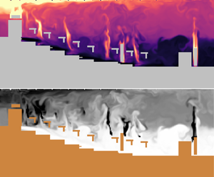
Snapshots and averaged steady-state temperature and CO $_2$ concentration maps are shown in figure 8. The snapshots show only the turbulent fluctuations and demonstrate that not only an averaged steady-state field is computed but also the transient evolution of the quantities. The slices on the bottom of figure 8 show the time-averaged temperature and CO $_2$ concentration. In the front part of the lecture hall one can see the characteristic separation layer seen in the one- and four-occupant simulations. Also, we observe that the CO $_2$ concentration is highest in the top rear part of the lecture hall.
The MILES results for the temperature (a) and for the CO $_2$ concentration (b) for the base case scenario of the lecture hall. The top row shows instantaneous snapshots and the bottom row time-averaged steady-state fields.

5.2 Spreading pattern
Figure 9 shows time-averaged steady-state exhaled air concentration maps for this scenario in the approximate breathing zone. The red dots denote the locations of selected emitters. The exhaled air from emitters sitting in the upper parts of the lecture hall (top end of the pictures) has a smaller domain of influence which is mainly limited to the upper region. The two emitters located on the side mainly spread towards the corners, whereas the exhaled air by the spreader in the middle is sucked up by the heat-induced airflow of the projector. The exhaled air from emitters sitting in the front part of the lecture hall, however, can spread much wider. Again, for the two spreaders at the sides, the exhaled air is mainly transported to the back and towards the corners of the lecture hall. The air exhaled in the middle of the front row is transported to both sides of the lecture hall with a preference for the right side. Streamlines for two of the locations are shown in figure 13.
Lecture hall base case: spread of exhaled air for different emitter locations in the lecture hall. The red dot in each panel depicts the location of the emitter. Note: the depicted slice is not perpendicular to the  $x_3$ axis but slanted because of the slanted room geometry.

To gain more confidence in these findings, the robustness of these results was examined by varying different simulation input parameters and by comparing the resulting spreading maps to the baseline case shown in figure 9.
5.3 Robustness of spreading patterns
The main modelling assumptions required for these simulations is the introduction of the source terms. We therefore study the robustness of the tracer spreading with respect to the heat input per occupant as well as the heat source-term distribution.
5.3.1 Heat input – qualitative effect
The heat transfer by the occupants is a major driver of the flow in such lecture halls. The heat output of one occupant in the box of the DNS was approximately  $12$ to $15$ W depending on the flow rate considered. However, typical values used for realistic studies are $\approx$80–130 W (Reference Spitzer, Hettinger and KaminskySpitzer, Hettinger & Kaminsky 1982) per occupant of which approximately 50 W are transferred via convection (Reference HöppeHöppe 1993). Here, we assumed that loss due to radiation gets absorbed by the walls where the added heat contributes very little to natural convection, thus it is ignored. The default spreading pattern in figure 9 is based on a heat flux of 42 W per occupant. Figure 10 shows the same spreading pattern for a heat flux of 15 W per person.
Lecture hall with different heat input: spread of exhaled air for different emitter locations in the lecture hall. Compared with the base case in figure 8, and figure 9 the heat input per occupant here is 15 W. The red dot in each panel depicts the location of the emitter. Note: the depicted slice is not perpendicular to the  $x_3$ axis but slanted because of the slanted room geometry.

For the rear part of the lecture hall, the spreading patterns in the top row of figure 10 look comparable to the ones for 42 W. The spreading patterns for the three locations in the front (bottom row of figure), however, are different compared with the baseline case. Especially further away from the source the magnitude is much reduced for the front left and front centre spreader. The spreader in the front right shows a unique feature of very high concentration towards the upper right corner similar to the pattern observed for the same spreader location in figure 9.
5.3.2 Heat input – quantitative effect
As the heat input per occupant is increased from 15 to 70 W, the room temperature increases (figure 11a,c,e) as well as the temperature around each simulated occupant (figure 11a,e). Additionally, the temperature gradient from the front to the rear of the lecture hall also increases (figure 11e). The large temperature values towards  $x_1=0$ are a result of the high temperatures established just below the ceiling in the back of the lecture hall where the projector provides a strong heat source (figure 11e). At the back of the room (figure 11c), individual simulated occupants can no longer be discerned from the spatially averaged steady-state temperature profiles, suggesting that the rear row analysed is above the mixing height of the room.
Average steady-state temperature (a,c,e) and C $O_2$ concentration (b,d,f) for different heat input values (15,42,70) W. All profiles are temporally averaged steady-state data spatially averaged over different regions: (a,b) averaged over slices $x_1\times x_3$, [7.5 m, 8 m] $\times$ [2.8 m, 3.2 m] for each value along $x_2$; (c,d) averaged over slices $x_1\times x_3$, [2.7 m, 3.2 m] $\times$ [4.45 m, 4.95 m] for each value along $x_2$; (e,f) averaged over slices along $x_2 \times x_3$ [2 m, 2.5 m] $\times$ (0.5 m region above head) for each value along $x_1$. More details about the region above the head can be found in § A.5 in the Appendix.

The concentration profiles (figure 11b,d,f) show less clear a trend than the corresponding temperature profiles. However, the simulation results suggest that the peak tracer concentrations are highest for the lowest heat input per person (15 W) explored. The lower heat input per person results in a lower plume velocity and hence higher residual concentrations, although the relative effect seems small.
The layering height in the lecture hall is estimated by revisiting the (1.1) in Reference Yang, Ng, Chong, Verzicco and LohseYang et al. (2022) derived from Reference SchmidtSchmidt (1941), Reference Morton, Taylor and TurnerMorton, Taylor & Turner (1956) and Reference Linden, Lane-Serff and SmeedLinden et al. (1990)
 \begin{equation} \tilde{Q} = cn^{2/3}B^{1/3}(h-h_v)^{5/3}, \end{equation}
where  $n$ is the number of occupants, $B$ is the buoyancy flux per occupant, $h_v$ is the virtual origin and $c$ is an empirical constant ( $c = 0.105$ according to Reference Morton, Taylor and TurnerMorton et al. 1956; Reference LindenLinden 1999). Rearranging (5.1), we obtain the dependency of the cleaning height $h$ as a function of the number of occupants $n$ and the buoyancy flux per occupant $B$, as
 \begin{equation} h = \left(\frac{\tilde{Q}}{cn^{2/3}B^{1/3}}\right)^{3/5} + h_v. \end{equation}
We compare our simulated layering heights with the theoretically predicted values by (5.2). Figure 12 shows average steady-state profiles of temperature (a) and concentration (b) in the front part of the lecture hall.
Simulated average steady-state profile and predicted cleaning height of temperature (a) and CO $_2$ concentration (b). The simulated profiles (solid lines) are obtained from a slice at around $x_2 = 7.4$ m and between approximately $10.75\ m\leq x_1 \leq 13.27\ m$. The dot in the left panel denotes the cleaning height defined by the steepest temperature gradient. The dashed lines represent the predicted cleaning heights from (5.2). Spatially averaged profiles of temperature in the front part of the lecture hall for two different resolutions (c). The profiles are obtained from a slice around $x_2 = 7.4$ m and for $x_1$ between approximately 10.75 and 13.27 m.

In our simulations, we define the layering height as the point of steepest gradient in temperature, as depicted as a dot in the temperature profile in figure 12. The theoretically predicted layering height is shown by the dashed horizontal lines. The latter were obtained from (5.2) with  $n= 63, \tilde {Q} ={\frac {4500}{3600}}$ m $^3$ s $^{-1}$, $B = \{15+\frac {1200+500}{63},42+\frac {1200+500}{63},70+\frac {1200+500}{63}\}$ W. The constant contribution of the projector and mediastation, 1200 and 500 W, respectively, were added proportionally to $B$, thus increasing the heat flux per occupant by $(1200+500)/63$ W. The virtual origin height $h_v$ was chosen to be $h_v = -1.214$ m to match the cleaning height for a heat input of 42 W per occupant. The same value was then used for the cases of $15$ and 70 W.
5.4 Slightly perturbed seating scenarios
To check the robustness of the spreading patterns with respect to slightly perturbed seating configurations, we performed two additional simulations with 42 W per person. We compared the base case seating configuration shown in figure 32(a) with the two scenarios in figure 32(b,c). From the results in figure 33, it becomes clear that these slight perturbations in seating configuration and number of occupants do not have a strong effect on the resulting magnitude of the average profiles of temperature and CO $_2$ concentration. However, when moving all occupants positions by one seat as in scenario 1 in figure 32(b), we can clearly see the local changes of areas of high temperature and CO $_2$ concentration.
5.5 Projector
We also compared results of scenarios with and without the projector. The results are presented in figure 34 in § A.13. Surprisingly, despite the fact that the projector is by far the strongest heat source in the lecture hall, the profiles of temperature and CO $_2$ are even less affected than due to the slight perturbations discussed above. The largest difference is visible at the very back of the lecture hall (figure 34e), where the projector provides a strong heat source. The profiles in figure 34, however, do not cover much of the uppermost part of the lecture hall, where we would expect a stronger effect.
5.6 Resolution
We also show that, with respect to the mean temperature profile, the resolution of  $h = \Delta x = \Delta y = \Delta z = 0.05$ m is sufficient for this lecture hall simulation case. Figure 12(c) shows the spatially averaged temperature profiles in the front part of the lecture hall for resolutions of both $h = 0.0$ and 0.025 m. Both lines are averaged from 114 snapshots between 30 and 45 min of physical time.
5.7 Streamlines and flow structures
For a better understanding of how the spreading patterns above emerge, we show streamlines of the time-averaged steady-state velocity field, initialized at two of the 6 spreader locations in figure 9. We would like to point out that these are streamlines and not trajectories obtained by particle tracking. However, using frequent snapshots of the MILES solution for particle tracking would be an ideal extension and usage of the method. The streamlines in figure 13(a) show the spread of the exhaled air from the middle position of the front row. They are first going up but do not go all the way to the ceiling, indicating that the buoyancy force is not strong enough to push all the way through the warm upper layer. They are then mostly going towards the front of the lecture hall. These streamlines going to the front are then deflected to both sides of the lecture hall. The ones deflected towards the mediastation are sucked upwards by the flow due to the heat released by the mediastation in the front left corner. The other streamlines deflected to the other side return from the front wall and propagate towards the seating area in the front right corner, leading to an elevated concentration, as shown in bottom centre of figure 9. Figure 13(b) shows the spread of exhaled air from a second front row release position on the far right (bottom right corner in figure 9). Different from the release position in figure 13(a), the streamlines mostly occupy only the right side of the lecture hall, which explains to first order the higher concentration in exhaled air in the right part of the lecture hall in figure 9.
(a) Streamlines based on the averaged steady-state flow field. The streamlines are initialized at the location of the spreader in the middle of the front row shown in figure 7. (b) Streamlines based on the averaged steady-state flow field. The streamlines are initialized at the location of the spreader on the right end of the front row shown in figure 7.

These streamlines are based on the time-averaged velocity field, it is therefore not clear how stable the streamline path is over time.
6. Limitations
We provide a summary of the limitations of the present study regarding the physical assumptions and numerical discretizations used.
First, the physical limitations are listed. These include the fact that no active exhalation is taken into account; the multiphase nature of the exhalation is also not modelled with exhalations treated as passive tracers; the over-temperature and the momentum of the exhaled air are neglected. Compared with heat/temperature, the CO $_2$ exhalation is simplified more drastically in the MILES model, which could explain the larger differences in the agreement between DNS and MILES for the CO $_2$ concentration values and profiles observed in figures 3 and 4. Also, the radiation is not modelled explicitly but simply accounted for via an empirical reduction in the convective heat loss term (Reference Hardy and DuBoisHardy & DuBois 1937; Reference HöppeHöppe 1993). The fact that in reality the exhaled air is multiphase in nature, at core body temperature, which is significantly higher than the clothing temperature or temperature of the surrounding, and carries forward momentum, all significantly influence the tracer and pathogen distribution (Reference Bourouiba, Dehandschoewercker and BushBourouiba et al. 2014). All this can be modelled with an Euler–Lagrangian approach as done in Reference Chong, Ng, Yang, Verzicco and LohseChong et al. (2021) and Reference Ng, Chong, Yang, Li, Verzicco and LohseNg et al. (2021) but this is computationally much more costly, so that at most seconds of a single respiratory event can be modelled.
Second, we list the numerical scheme limitations. The simulations we show have an implicit turbulence model tightly coupled to the spatial discretization and therefore grid resolution. We had to use a higher grid resolution of  $300^3$ for the flow rate of $\tilde {Q}=0.04$ m $^3$ s $^{-1}$ compared with $150^3$ for $\tilde {Q}=0.09$ m $^3$ s $^{-1}$ to get better agreement with the DNS data. Moreover, for some simulations, we observe spurious spatial oscillations towards the ceiling of the lecture hall. From figure 23 in the Appendix, we have some indication that these oscillations become smaller with increasing grid resolution.
7. Conclusion and outlook
Motivated by the COVID-19 pandemic and the goal to help mitigate the risk of respiratory infectious disease transmission, a number of numerical studies on indoor ventilation have emerged recently (Reference VuorinenVuorinen et al. 2020; Reference Liu, He, Shen and HongLiu et al. 2021; Reference Talaat, Abuhegazy, Mahfoze, Anderoglu and PorosevaTalaat et al. 2021; Reference OksanenOksanen et al. 2022; Reference Wang and HongWang & Hong 2023; Reference Korhonen, Laitinen, Isitman, Jimenez and VuorinenKorhonen et al. 2024). Detailed LES simulation results (Reference Liu, He, Shen and HongLiu et al. 2021) for the Guangzhou restaurant scenario (Reference BostockBostock 2020; Reference ChangChang 2020) have shown a connection between regions of high aerosol exposure due to airflow inhomogeneity and reported infections, as well as the usefulness of computational fluid dynamics as an instrument for the estimation of airborne infection risk. Reynolds-averaged Navier–Stokes (RANS) results have been presented for a very similar case as the validation case used here with a single mannequin in a box (Reference Wang and HongWang & Hong 2023). The saturation of the interface height as a function of the ventilation rate agree very well with the results from Reference Yang, Ng, Chong, Verzicco and LohseYang et al. (2022). However, both Reference Liu, He, Shen and HongLiu et al. (2021) and Reference Wang and HongWang & Hong (2023) use a fixed temperature boundary condition for the people in the simulations, which does not allow for a control of the heat flux compared with the fixed heat flux condition used in this work. Different Dirichlet temperature values were used in Reference Auvinen, Kuula, Grönholm, Sühring and HellstenAuvinen et al. (2022) for the head and the clothing estimated from infrared images. The highly resolved LES simulations of a big room ( $V=170$ m $^3$, 286 million cells) are combined with aerosol concentration measurements to successfully validate the LES model and study two different strategies to reduce the transmission risk (Reference Auvinen, Kuula, Grönholm, Sühring and HellstenAuvinen et al. 2022). However, to simulate 1 h of physical time, the simulations take 6 days on more than 800 CPUs. Our method, using a coarser resolution as compared with Reference Auvinen, Kuula, Grönholm, Sühring and HellstenAuvinen et al. (2022), can simulate a 1 hour lecture hall scenario of the same order of magnitude in size ( $V=580$ m $^3$, 7.1 million cells) on a single GPU in less than 24 h using the latest GPU hardware. There are other existing fast LES simulations (Reference Khan, Delbosc, Noakes and SummersKhan et al. 2015; Reference Kristóf and PappKristóf & Papp 2018; Reference Bauweraerts and MeyersBauweraerts & Meyers 2019; Reference Adekanye, Khan, Burns, McCaffrey, Geier, Schönherr and DorrellAdekanye et al. 2022). Most of them rely either on a conventional LES approach using subgrid-scale models, make use of a different method such as the lattice Boltzmann method or require more involved computations. Also, none of these methods uses the source-term approach employed here to model the heat loss of the occupants. RANS has also been used for efficient simulation of the flow inside an aircraft cabin (Reference Talaat, Abuhegazy, Mahfoze, Anderoglu and PorosevaTalaat et al. 2021). However, the authors do not mention temperature being taken into account, which would be important to capture buoyancy effects driven by the heat loss of the people. In Reference VuorinenVuorinen et al. (2020), coughing is modelled and the momentum transfer by the cough is accounted for. Long-range transport $O$(10 m) of aerosols is shown. For the OpenFOAM simulations, an implicit LES approach was used as a subgrid-scale model (Reference VuorinenVuorinen et al. 2020), similar to the MILES approach used here. Recently, a highly efficient GPU-based LES simulation tool that uses binary masks very similar to the ones used here has been reported (Reference Korhonen, Laitinen, Isitman, Jimenez and VuorinenKorhonen et al. 2024). Despite the high efficiency, no cases with physical simulation duration greater than 30 min are presented. Here, we have presented a newly developed MILES code for ventilation simulation. This simple yet reasonably accurate numerical scheme, and especially its powerful implementation with the use of PyTorch (Reference PaszkePaszke et al. 2019) (earlier version) or Julia (Reference Bezanson, Edelman, Karpinski and ShahBezanson et al. 2017; Reference Omlin and RässOmlin & Räss 2022) (current version) for GPUs, make the new code a potentially valuable tool for flow simulation indoors. The use of source terms for heat and scalar concentration in the form of binary masks was shown to be a possible way to avoid the high computational cost related to boundary layers with Dirichlet conditions for temperature and scalar concentration. The technique of the modelling via source terms is not restricted to a MILES method. It could be similarly used together with conventional LES approaches. We compared the MILES results with DNS data by Reference Yang, Ng, Chong, Verzicco and LohseYang et al. (2022) for displacement ventilation in a room with single and multiple occupants. Good qualitative agreement can be observed for temperature, CO $_2$ and velocity profiles. Moreover, we illustrate the application of MILES to a lecture hall.
The sensitivity of tracer spreading to the choice of values for various modelling parameters, such as heat input per occupant and heat layer thickness around the occupants, was investigated. The effects on temperature and CO $_2$ concentration values resulting from an increased heat layer thickness from $h=0.05$ to 0.1 m for the lecture hall case are small, where the larger thickness tends to smooth out peaks. This can be explained by the fact that the larger heat release layer has a more spread out heat source term which is smaller in numerical magnitude per cell because the source term is applied in more cells. For the two different cases we found that the effect of the heat layer thickness on the spreading pattern in the lecture hall is negligible. A change in the heat input of between 15 and 70 W showed a direct effect of increased temperature values in the lecture hall.
Generally, a potentially infected host, i.e. the source, sitting in the back typically influences a small region, mostly bounded by the rear of the lecture hall. The exhaled air of a source sitting in the front is transported up and to the back, resulting in predominantly increased concentrations toward the back. If one were to extrapolate the flow and concentration of the tracer to the flow and concentration of pathogen-bearing exhalation droplets or droplet residues, the simulations would suggest that people sitting in the back of the lecture hall are exposed to higher concentrations of exhaled air and therefore experience a higher risk of infection, compared with people in the front. Thus, occupants in the back would have a higher risk of exposure compared with the well-mixed limit, and people seated at the front a lower risk of exposure, again compared with the well-mixed limit. These results, from MILES, are supported qualitatively by recent experiments by Reference Rusch and RösgenRusch & Rösgen (2022), who used direct measurements of CO $_2$ with human subjects present in lecture halls of similar geometry and ventilation type as examined here. Their measurements also show increased scalar concentrations in the back of slanted auditoriums, further demonstrating concentration inhomogeneity, providing further evidence that the well-mixed limit is not a suitable approximation for risk assessment and mitigation of airborne contaminants and pathogens in key gathering locations such as auditoriums, movie theatres, etc.
Further, on the fluid dynamics front, a very interesting aspect and one of general importance is the amount of heat an occupant introduces to the flow. The values in the DNS resulting from isothermal surfaces at 27  $^\circ$C range from 12 to 15 W per occupant, which is much lower than expected based on experience (Reference Craven and SettlesCraven & Settles 2006; Reference Bhagat and LindenBhagat & Linden 2020). Our sensitivity studies show that the exact heat flux value might not have a huge effect on concentration maps obtained for the entire lecture hall. They also show that a change in heat input has a direct effect on temperature values and via buoyancy also on CO $_2$ concentrations. It would be of interest to obtain the DNS results using a prescribed heat flux condition. One could then study both the effect of the boundary condition itself but also further validate the MILES approach for these applications.
Finally, studies using our MILES method should be performed to explore a wider parameter space, e.g. the geometry of the lecture hall, the ventilation type, the movement of bodies (Reference Mingotti, Wood, Noakes and WoodsMingotti et al. 2020) and different respiratory activities. One direct extension of the work could involve producing frequent MILES solution snapshots and using the resulting flow fields for a particle tracking study. Furthermore, additional studies are necessary to investigate to which degree CO $_2$ concentration and the concentration of exhaled droplet residues actually correlate, which remains a major unknown. In addition, validation of simulation results against measured CO $_2$ or droplet/particle concentrations is also necessary to ensure that the simulations correctly incorporate the essential physics to capture the flow and transport of exhalations. These factors are crucial for better understanding building ventilation systems in general and how they can be leveraged for improved infection risk mitigation.
Acknowledgements
The authors thank T. Rösgen and A. Rusch (ETH Zürich) for numerous constructive discussions. The authors thank B. Zoller (Air Flow Consulting) for the many constructive discussions. The authors thank the ETH Facility Services and Engineering and Systems Departments for their kind support and good collaboration. Some of the computing for this project was performed on the Sherlock cluster. We would like to thank Stanford University and the Stanford Research Computing Center for providing computational resources and support that contributed to these research results. We acknowledge PRACE for awarding us access to Irene at Tres Grand Centre de Calcul (TGCC) du CEA, France (project 2020235589 and project 2021250115). This work was also carried out on the Dutch national e-infrastructure with the support of SURF Cooperative. We also thank the support from the project MItigation STrategies for Airborne Infection Control (MIST). The figures in this manuscript have been generated with the help of Matplotlib (Reference HunterHunter 2007) and Mayavi (Reference Ramachandran and VaroquauxRamachandran & Varoquaux 2011).
Funding statement
D.L., R.V. and R.Y.: this publication is part of the project MItigation STrategies for Airborne Infection Control (MIST) with project number P20-35 of the research programme Perspectief, which is (partly) financed by the Dutch Research Council (NWO). L.B. acknowledges partial support from the US National Science Foundation, MIT-IBM Watson Lab, and the Fluids and Health's Healthy Teaching Project support by the MIT-Sloan School, the US National Institutes of Health, and the US Centers for Disease Control and Prevention (CDC)'s National Institute for Occupational Safety and Health (NIOSH). P.J., L.M. and N.M.L. acknowledge ETH internal funding.
Declaration of interests
The authors declare no conflict of interest.
Author contributions
Conceptualization: N.M.L., L.B. and P.J.; data curation: N.M.L. (lead) and R.Y. (supporting); formal analysis: N.M.L., R.Y., L.B. and P.J.; funding acquisition: P.J., R.V., D.L. and L.B.; investigation: N.M.L. (lead) and R.Y. (supporting); methodology: N.M.L., R.Y., L.M., R.V., D.L., L.B. and P.J.; resources: P.J.; software: N.M.L. (lead), L.M. and P.J. (supporting); supervision: R.V., D.L., L.B. and P.J.; validation: N.M.L. and R.Y.; visualization: N.M.L.; writing – original draft: N.M.L.; writing - review and editing: N.M.L., R.Y., L.B., L.M., R.V., D.L. and P.J.
Data availability statement
The data that support the findings of this study are available from the corresponding author, N.M.L., upon reasonable request.
Ethical standards
The research meets all ethical guidelines, including adherence to the legal requirements of the study country.
Appendix A
A.1 The MILES method and numerical discretization
The approach used in this paper can be categorized as a MILES method (Reference Boris, Grinstein, Oran and KolbeBoris et al. 1992; Reference Grinstein, Margolin and RiderGrinstein et al. 2007), which belongs to the larger class of implicit LES models (Reference Margolin, Rider and GrinsteinMargolin et al. 2006). In contrast to a conventional LES method, there is no explicit subgrid-scale model. Instead, an implicit model originating from the numerical diffusion of the discretization scheme is used (Reference BorisBoris 1989; Reference Boris, Grinstein, Oran and KolbeBoris et al. 1992; Reference Margolin, Rider and GrinsteinMargolin et al. 2006).
We expect the MILES method to work in this context since the simulated ventilation flows are not dominated by near-wall turbulence, in which case it would be very expensive to use a MILES method. Recently, an implicit LES approach using OpenFOAM has been used for the modelling of aerosol transport (Reference VuorinenVuorinen et al. 2020). We further reduce the influence of detailed geometrical features or surface boundary conditions by using appropriate source terms. Both classical LES as well as MILES work very well for high Reynolds number free-shear flows Reference Grinstein, Margolin and RiderGrinstein et al. (2007, Chapter 8) and Reference Fureby and GrinsteinFureby & Grinstein (1999). With both methods, it is difficult, however, to properly describe wall-bounded flows or boundary layers (Reference Piomelli and BalarasPiomelli & Balaras 2002). One would need high local grid refinements in the vicinity of occupants as well as walls to properly capture the boundary layers and the associated heat transfer in these regions. To circumvent such expensive refinements, we use source terms for both heat and scalar variables instead of prescribing the values at the boundary using Dirichlet conditions. This is also more physiological as discussed in the introduction in the context of surface temperature.
The fact that we use a uniform grid resolution in each direction and that we use masks to apply source terms and boundary conditions allow for a very simple data structure and compact operations using tensor slicing.
A.1.1 Numerical algorithm
The following algorithm describes the solution procedure for the MILES method. The different indices  $i,j,n$ refer to the velocity component, a summation index and the timestep index respectively. The space discretization is not explicitly given and is implicitly shown through the fact that we use $\delta$ instead of $\partial$ to denote the numerical approximation of the derivative.
Algorithm for simulation of buoyancy-driven flows with MILES

A.1.2 Pressure Poisson equation
For the solution of the pressure Poisson equation, we use a simple Jacobi iteration with a constant number of iterations. For the cases with the  $3\ {\rm m} \times 3\ {\rm m} \times 3\ {\rm m}$ box (1 and 4 people), we used 50 iterations and for the lecture hall simulations, we used 100 iterations.
A.2 Details of the second-order upwinding scheme
We use a second-order upwind discretization for the convective terms, second-order central discretization for the viscous and diffusion terms and a first-order Euler forward time integration. For second-order upwinding of the convective terms we use a slope advection technique used in Reference Kulka and JennyKulka & Jenny (2022), which is uncommon and will therefore be explained in more detail next. Figure 14 depicts an interface between two cells (left and right) with cell centres denoted by  $x_L$ and $x_R$, respectively. We will describe the special case of a flow from left to right (i.e. where ${(u_L^n+u_R^n)}/{2}\geq 0$; blue arrow in figure 14). The case with a flow from right to left can be treated analogously. To compute the convective flux of a quantity $\phi$ across the interface at $x_F$, we need an estimate of $\phi (x = x_F)$, where $\phi$ can either be one of the three velocity components, a temperature value or a passive scalar concentration. To estimate $\phi (x = x_F)$ we use
 \begin{equation} \phi(x = x_F) = \phi_{L}^n + \sigma (\phi_{LL}^n,\phi_{L}^n,\phi_{R}^n)\left((x_{F}-x_{L})-{\frac{\Delta t}{2}u_{F}^n}\right), \end{equation}
where  $u_F^n = 1/2(u_L^n+u_R^n)$ and $\sigma (\phi _{LL}^n,\phi _{L}^n,\phi _{R}^n)$ is a slope. We subtract $u_F^n \Delta t/2$ to provide an estimate at $t = t^{n+1/2}$ rather than at $t^n$. To avoid spurious oscillations, a limiter has to be applied. Here, we choose the Koren limiter (Reference KorenKoren 1993) to obtain the slope as
 \begin{equation} \sigma(\phi_{LL}^n,\phi_L^n,\phi_R^n) = \frac{\phi_{R}^n-\phi_{L}^n}{x_{R}-x_{L}}\max\left[0,\min\left(2r,\min\left(\frac{(1 + 2r)}{ 3},2\right)\right)\right], \end{equation}
where  $r = (\phi _{L}^n-\phi _{LL}^n)/(\phi _{R}^n-\phi _{L}^n)$.
Graphical illustration of the second-order upwinding scheme using slope advection. The flow is from left to right (blue arrow). The quantity  $\phi$ at the interface $x_F$ is then obtained by a slope reconstruction in the left cell. However, the value at the interface is not simply taken at the interface at $t = t^n$ but from the point $x_F - u_F{\Delta t}/{2}$ representing the average value at the interface during the timestep.

A.3 Geometry, boundary conditions and source terms
The computational domain for the case is the same as used by Reference Yang, Ng, Chong, Verzicco and LohseYang et al. (2022) (shown in figure 15). It is a  $3\ {\rm m}\times 3\ {\rm m}\times 3\ {\rm m}$ box with an inlet ( $3\ {\rm m}\times 0.3\ {\rm m}$) in the lower region ( $x_1 = 0,0\leq x_2\leq 3$ m, $0\leq x_3\leq 0.3$ m) and an outlet of the same size in the upper region ( $x_1 = 3$ m, $0\leq x_2\leq 3$ m, $2.7\ {\rm m}\leq x_3 \leq 3\ {\rm m}$). A Cartesian grid is used with equidistant spacing of $\Delta x_1 = \Delta x_2 = \Delta x_3 = 0.02$ m or $\Delta x_1 = \Delta x_2 = \Delta x_3 = 0.01$ m in all three directions. This translates into $150^3 = 3.375\times 10^6$ or $300^3 = 27\times 10^6$ grid cells. In comparison, the DNS used by Reference Yang, Ng, Chong, Verzicco and LohseYang et al. (2022) used a grid with $768^3 \approx 453\times 10^6$ cells.
Sketch of the domain set-up for the comparison against DNS (Reference Yang, Ng, Chong, Verzicco and LohseYang et al. 2022). The room/box is  $3\ {m}\times 3\ {m}\times 3\ {m}$ with an inlet (green) of height 0.3 m at the bottom of the front wall and an outlet (brown) of the same height at the ceiling of the back wall. The rest of the walls (grey) are adiabatic and impenetrable. The occupant is modelled by a solid adiabatic core (grey), a heat source shell (yellow) and an exhaled air source region (red).

The inlet and outlet velocities are constant and unidirectional along the  $x_1$-coordinate over the entire inlet and outlet areas. The inlet temperature $T_{in}$ is 22 $^\circ$C and the inlet CO $_2$ concentration is 400 ppm. The outlet velocity is specified to be the same as the inlet velocity and for temperature and scalar concentration, a zero-gradient condition is employed at the outlet. Impermeable and adiabatic no-slip boundary conditions were applied at the walls.
The occupant sitting in the room was modelled with a solid adiabatic surface surrounded by a thin layer of cells in which the occupant's heat production was introduced through the source term  $P$ in (2.1c). As already discussed, compared with the DNS, no Dirichlet boundary condition was set for the temperature of the occupant. Instead, we fixed the power transferred through heat conduction from the body into the fluid domain according to that resulting from the DNS. The differences in modelling the occupant and the associated source terms are shown in more detail in figure 16.
Modelling of the occupant's associated heat and scalar source in the DNS (a–c) and MILES (d–f). (a) Impenetrable body in the DNS simulation. (b) Fixed body clothing surface temperature (e.g. Dirichlet boundary condition) in the DNS. (c) Exhalation jet and CO $_2$ source term. (d) Impenetrable adiabatic surface for the MILES simulations. (e) Layer of cells around the body where the heat source (e.g. prescribed constant power output) is set in the MILES. (f) Region of a few cells representing the mouth of the occupant in the MILES simulations, where the scalar source term is set equivalent to the CO $_2$ exhalation rate.

Similarly to the heat input, the exhaled air of the occupant is modelled as a source term in the species equation assuming a constant volumetric flow rate of 7.5 l min $^{-1}$ and a CO $_2$ concentration of 4 %. The exhaled air is added as a passive tracer through the source term $S$ in (2.1d). The momentum transfer due to the exhalation is neglected, which is another major difference from the DNS in which the exhalation is modelled as a fully resolved pulsating jet (see supplementary materials of Reference Yang, Ng, Chong, Verzicco and LohseYang et al. 2022).
Table 2 lists all the different simulation cases together with the input values for the flow rate  $Q$, the heat source term $P$ and the scalar source term $S$.
$S$.
Input parameters for all simulation cases.

A.4 Radiative heat flux
We did not model the radiative heat transfer in the simulations. However, we choose a heat input of 42 W per person for the lecture hall simulations. This is motivated by Reference HöppeHöppe (1993), that provides a value of 48 W of convective heat loss for typical indoor conditions. The heat loss through radiation represents the major part of the total heat loss for environmental temperatures below 30  $^\circ$C (Reference Hardy and DuBoisHardy & DuBois 1937). Despite the fact that we did not include radiation, we want to show what values we would expect for the radiative heat flux between the person and the surroundings. Figure 17 shows the radiative heat flux from a single person to the wall for the simplified scenario of the $3\ {\rm m} \times 3\ {\rm m} \times 3\ {\rm m}$ box.
Radiative heat flux from the occupant to the walls in the domain. The occupant's surface area in cm $^2$ was calculated using the equation $94.9\times \textit{[}\text {weight (kg)}^{0.441}\textit{]} \times \textit{[}\text {height (cm)}^{0.655}\textit{]}$ from Reference Shuter and AslaniShuter & Aslani (2000) for a person of 65 kg and 1.75 m. The evaluated surface area is 1.76 m $^2$. The emissivity of the occupant is chosen as 0.89, which is a value for cotton (Reference CaiCai et al. 2017). The emissivity of the wall is chosen as 0.85, which is in the range of typical values for the emissivity of paint (Reference Fantucci and SerraFantucci & Serra 2020). The wall temperature is assumed to be fixed at 295 K. Since the view factor from the body to the wall is not easy to calculate, the figure shows the radiative heat flux as a function of the view factor and the body surface temperature of the occupant. A typical value for the view factor of a standing person is 0.7 (Reference HöppeHöppe 1993). We chose a range from 25 to 35 $^\circ$C for the clothing surface temperature based on Reference Zhang, Wang and LiZhang, Wang & Li (2010) and a meaningful range of the wall (environmental) temperature from 15 to 25 $^\circ$C.

A.5 Averaging regions
A.5.1 One person in a box case
Figure 3 includes averages computed in four different regions of the cut plane at  $x_2 = 1.5$ m. Figure 18 shows these different regions. Additionally, all profile data throughout the manuscript are obtained by averaging in the combined blue and yellow region of figure 18.
Definition of the averaging regions used in figure 3. The regions are all taken at the cell closest to  $x_2 = 1.5$ m in the middle of the domain.

A.5.2 Lecture hall case
Figure 19 shows the slanted averaging region in yellow that was used for the averages in figures 11(f), 21(f), 33(f) and 34(f).
An  $x_1-x_3$ slice of the lecture hall with the solid object geometries (dark violet), the region above the people (yellow) and the remaining cells (green). The yellow cells are taken into account for the average in figures like 11(e,f). In the $x_2$ direction, $x_2 \in \textit{[}2\ {m}, 2.5\ {m}\textit{]}$ was used.

A.6 Size of heat release layer around the person
One important modelling parameter of the MILES simulations is the size of the heat release layer surrounding the person. For the 1 person in a box case, we simulated three cases with  $Q = 0.04$ m $^3$ s $^{-1}$ but with varying thickness of the heat release layer. For the lecture hall scenario, we compared the 1 cell layer thickness used in all simulations for the lecture hall with a 2 cell layer thickness. For both the case with one person in a box and the lecture hall, the heat released in the layer was kept constant and only the size of the layer (i.e. number of cells where the source term is applied) was changed. Figure 20 shows the influence of the heat release layer thickness on the resulting average temperature profile. In the simulations for one person in a box, we chose to use the 3 cell layer thickness because, for $\Delta x = 0.02$ m and $Q=0.04$ m $^3$ s $^{-1}$ person $^{-1}$, it compared best with the DNS results. In the lecture hall simulations, we chose a heat layer thickness of 1 cell layer. Furthermore, figure 21 shows the differences between 1 and 2 cell layers for the heat release thickness for different profiles in the lecture hall scenario. One observation from figure 21 is the fact that the thicker heat layer tends to smooth out peaks in both the temperature and CO $_2$ profiles. This can be explained by the fact that the thicker heat release layer has a more spread out heat source term which is smaller in numerical magnitude per cell because the source term is applied to more cells. Finally, note that in the 4 person case, we used a resolution of $nx = 150^3$ and a heat layer thickness of 2 cell layer thicknesses (i.e. $2 \times 0.02\ {\rm m}$).
Profiles of average temperature over the height of the room for different heat release layer thickness values. (a) Shows three different thickness values for the case with one person in a box. The average is computed at every height from the blue and yellow regions in figure 18. (b) Shows two different thickness values for the lecture hall case. The profiles are obtained from a slice at around  $x_2 = 7.4$ m and in the range of approximately $10.75\ {m}\leq x_1 \leq 13.27\ {m}$ in the lecture hall.

Average steady-state temperature (a,b,c) and C $O_2$ concentration (d,e,f) for two different values of the thickness of the heat release layer around the people. All profiles are temporally averaged steady-state data spatially averaged over different regions: (a,d) averaged over slices $x_1\times x_3$, [7.5 m, 8 m] $\times$ [2.8 m, 3.2 m] for each value along $x_2$; (b,e) averaged over slices $x_1\times x_3$, [2.7 m, 3.2 m] $\times$ [4.45 m, 4.95 m] for each value along $x_2$; (c,f) averaged over slices along $x_2 \times x_3$ [2 m, 2.5 m] $\times$ (0.5 m region above head) for each value along $x_1$. More details about the region above the head can be found in § A.5 in the Appendix.

A.7 Grid convergence
We performed a grid convergence study for the case with one person in the box for flow rates of  $Q = 0.01$, 0.04 and $Q= 0.09$ m $^3$ s $^{-1}$. Figure 22 shows the steady-state temperature profile in the middle slice of the domain. For the intermediate and high flow rate cases, no strong dependency on the grid resolution is visible. For the lowest flow rate, the solution converges for $150$ grid cells in each direction. However, figure 22 can be misleading. When looking at the steady-state-averaged temperature profile for different grid resolutions, we can see the influence of the grid resolution more clearly. We see that, for the highest flow rate, the profile agrees well with the DNS data and seems to be converged. For the intermediate flow rate, we see that a resolution of $n_x^3 = 300^3$ yields a much better agreement with the DNS profile than the lower resolutions. For the lowest flow rate, also the profile data converge with $150$ grid cells in each direction.
Mean temperature in the middle slice of the one person case as a function of number of grid cells. Different colours represent different flow rates. The error bars denote the maximum and minimum values observed during the 200 snapshot averaging period.

Steady-state temperature profile in the middle slice of the domain for the 1 person case. (a–c) Show different flow rates and the different colours denote different grid resolutions. The red lines show the DNS profile of Reference Yang, Ng, Chong, Verzicco and LohseYang et al. (2022).

A.8 Conservativeness
To check whether our code is fully conservative, we compared the outlet temperature in the steady state with the one obtained from an idealized model, assuming perfectly mixed conditions in the lecture hall.
Temporal evolution of average and outlet temperature in the ML E12 lecture hall for the base case configuration. The black dashed line shows the result of a perfectly mixed room according to (A3). The blue and orange curves show the simulated outlet and average room temperature, respectively.

Evolution of the temperature in the middle slice of the domain (i.e.  $0.0\leq x_1\leq 1.0$ m and $1.87\leq x_1\leq 3.0$ m which is equivalent to the the blue and yellow areas in figure 18 combined) for three different flow rates for the one person in the box case. Note: here T refers to a dimensional temperature in Kelvin, $T_0 = 295\ {K}$ and $T_\infty$ is the steady-state temperature reached in Kelvin.

Evolution of the temperature in the middle slice of the domain (i.e.  $0.0\leq x_1\leq 1.0$ m and $1.87\leq x_1\leq 3.0$ m which is equivalent to the the blue and yellow areas in figure 18 combined) for three different flow rates for the one person in the box case. Note the non-dimensional $x$ axis which plots $t/\tau$, where $\tau = V/\dot {V} = 1/a$ is the exponential time constant from the well-mixed model in (A6). Note: here T refers to a dimensional temperature in Kelvin, $T_0 = 295\ {K}$ and $T_\infty$ is the steady-state temperature reached in Kelvin. Note that $T_\infty$ is different for the different cases.

Evolution of the temperature in the middle slice of the domain (i.e.  $0.0\leq x_1\leq 1.0$ m and $1.87\leq x_1\leq 3.0$ m which is equivalent to the blue and yellow areas in figure 18 combined) for three different flow rates for the one person in the box case. Note the non-dimensional $x$ axis which plots $t/\tau$, where $\tau = V/\dot {V} = 1/a$ is the exponential time constant from the well-mixed model in (A6). Note: here T refers to a dimensional temperature in Kelvin, $T_0 = 295\ {K}$ and $T_\infty$ is the steady-state temperature reached in Kelvin. Note that $T_\infty$ is different for the different cases.

Qualitative comparison of the steady-state fields for  $Q = 0.01$, 0.04, 0.09 m $^3$ s $^{-1}$; time-averaged DNS (a–c) and time-averaged MILES (d–f). (a–f left panel) For each flow rate we show the temperature in a slice through the middle of the domain (i.e. around $x_2 = 1.5$ m). (a–f right panel) For each flow rate weshow the velocity in the horizontal direction in a slice through the middle of the domain (i.e. around $x_2 = 1.5$ m).

Profiles of average temperature (a) and CO $_2$ concentration (b) in the middle slice around $x_2 = 1.5$ m over the height of the room for flow rates $Q = 0.01$, 0.04, 0.09 m $^3$ s $^{-1}$ person $^{-1}$. The solid lines show the DNS and the dashed lines the MILES results. The average is computed at every height from the blue and yellow regions in figure 18. More details about the averaging regions are given in § A.5 of the Appendix.

Transient evolution of the temperature profile. The three different panels show three different flow rates. The lighter the lines, the earlier in time they were averaged. The red lines show the DNS profile of Reference Yang, Ng, Chong, Verzicco and LohseYang et al. (2022).

Streamlines in a slice of the lecture hall for three different heat inputs per occupant; (a) 15 W, (b) 42 W, (c) 70 W.

We estimate the temporal evolution of the mean dimensional temperature  $\bar {T}$ in the lecture hall via an energy balance. The balance equation for the temporal evolution of the mean temperature can be written as
 \begin{align}
\underbrace{c_p\times V\times \rho \frac{{\rm d} \bar{T}}{{\rm
d}t}}_{\mathit{change\ of\ thermal\ energy\ in\ the\ room}}
= \underbrace{\dot{q}_{{bodies}}}_{\mathit{heat\ loss\ of\ people}}-\underbrace{\dot{V}\times \rho \times c_p
\bar{T}}_{\mathit{heat\ loss\ throughout\ flow\ at\ the\ ceiling}} + \underbrace{\dot{V}\times \rho \times c_p
T_{in}}_{\mathit{heat\ input\ through\ fresh\ air}}, \end{align}
\begin{align}
\underbrace{c_p\times V\times \rho \frac{{\rm d} \bar{T}}{{\rm
d}t}}_{\mathit{change\ of\ thermal\ energy\ in\ the\ room}}
= \underbrace{\dot{q}_{{bodies}}}_{\mathit{heat\ loss\ of\ people}}-\underbrace{\dot{V}\times \rho \times c_p
\bar{T}}_{\mathit{heat\ loss\ throughout\ flow\ at\ the\ ceiling}} + \underbrace{\dot{V}\times \rho \times c_p
T_{in}}_{\mathit{heat\ input\ through\ fresh\ air}}, \end{align}
where  $c_p$ is the heat capacity of air, $V$ is the fluid volume of the lecture hall, $\rho$ is the air density, $\dot {V}$ is the volumetric inflow and outflow rate and $T_{in}$ the temperature of the fresh air inflow. Equation (A3) can be re-written in a more compact form as
 \begin{equation} \frac{{\rm d}u}{{\rm d}t} = {-}au + b,\quad u(t = 0) = u_0, \end{equation}
with the solution
 \begin{equation} u(t) = \frac{b}{a} + \left(u_0-\frac{b}{a}\right){\rm e}^{{-}at}. \end{equation}
For the energy balance in (A3), we have
 \begin{equation}
a = \frac{\dot{V}}{V}, \quad b = \frac{\dot{q}_{{bodies} }}{c_p\times V \times \rho}
+ \frac{\dot{V}}{V}T_{in}. \end{equation}
\begin{equation}
a = \frac{\dot{V}}{V}, \quad b = \frac{\dot{q}_{{bodies} }}{c_p\times V \times \rho}
+ \frac{\dot{V}}{V}T_{in}. \end{equation}
In figure 24 we compare the temporal evolution according to (A3) with the simulated values for both outlet and average room temperatures. The outlet temperature of the simulation must match the steady-state temperature from the zero-dimensional model, since the energy intake and sources in the lecture hall must be balanced at the outlet in both cases. The difference between the simulated mean and the outlet temperature indicates that these flows in the lecture halls are in fact not well mixed but exhibit heterogeneous structures; the most prominent one is a vertical thermal stratification.
Set-up for slightly perturbed cases. Except for the arrangement of the occupants, all parameters are constant. (a) The base case configuration used in figures 9 and 11. The number of occupants in the base case is 63 including the lecturer, not visible here. (b) The first perturbed scenario, where occupants are sitting on the seats that were empty in the base case. The number of occupants is 62 including the lecturer, not visible here. (c) The second perturbed scenario, where occupants are sitting directly behind each other whereas they are sitting diagonally apart in the two other cases. The number of occupants is 66 including the lecturer, not visible here.

Average steady-state temperature (a,c,e) and C $O_2$ concentration (b,d,f) for the three perturbed cases in 32. All profiles are temporally averaged steady-state data spatially averaged over different regions: (a,b) averaged over slices $x_1\times x_3$, [7.5 m, 8 m] $\times$ [2.8 m, 3.2 m] for each value along $x_2$; (c,d) averaged over slices $x_1\times x_3$, [2.7 m, 3.2 m] $\times$ [4.45 m, 4.95 m] for each value along $x_2$; (e,f) averaged over slices along $x_2 \times x_3$ [2 m, 2.5 m] $\times$ (0.5 m region above head) for each value along $x_1$. More details about the region above the head can be found in § A.5 in the Appendix.

A.9 Time to steady state
One important aspect to consider that we observed when performing these simulation studies is the fact that it can take a considerate amount of physical time for a flow to reach the steady state. From the well-mixed scenario, the time to reach the steady state is inversely proportional to the flow rate  $\dot {V}$. Figures 25 and 26 show the temporal evolution of the non-dimensional temperature in the middle slice of the domain for three different flow rates in hours and non-dimensional time, respectively. The lowest flow rate case follows almost the same trajectory to the steady state as the analytical well-mixed scenario whereas the intermediate and high flow rate converge to the steady state faster than the well-mixed solution. Figure 27 is the same as figure 26 but includes simulations at different resolutions as well.
A.10 Steady-state fields and profiles and transient profiles
Figure 28 shows steady-state-averaged fields for the three flow rates of  $Q = 0.01,0.04$ and 0.09 m $^3$ s $^{-1}$. Differently from figure 1, it includes the data for the lowest flow rate. Figure 29 shows steady-state-averaged profiles for the three flow rates of $Q = 0.01$, 0.04 and 0.09 m $^3$ s $^{-1}$. Differently from figure 4, it includes the data for the lowest flow rate. The agreement for the lowest flow rate is much worse compared with the agreement for the intermediate and high flow rates. One possible explanation for this is that it takes approximately 4 h to reach the steady state for the low flow rate case, as shown in § A.9, and given the cost of the DNS as shown in table 1, it is not feasible for the DNS profiles to be extracted after a full simulation up to 4 h. We therefor also looked at the profile evolution over time in the MILES simulation to check whether a profile at an earlier instance in time agrees better with the DNS profile. As shown in figure 30, the profiles for $Q = 0.04$ and 0.09 m $^3$ s $^{-1}$ converge quite quickly to the steady-state value. This is in agreement with figures 25 to 27. For $Q = 0.01$ m $^3$ s $^{-1}$, we see a slow build up of the profile over the course of the simulation. Every line is obtained in a new averaging window of approximately 14 min. The best agreement with the DNS data is obtained with the profile obtained between approximately 42 and 56 min.
A.11 Streamlines for different occupant heat release rates in the lecture hall
Figure 31 shows time-averaged streamlines for different heat release rates of the occupants in the lecture hall.
A.12 Slightly perturbed scenarios
We ran two additional cases where, compared with the base case, we slightly perturbed the seating configurations in the lecture hall. Figure 32 shows the set-up for the three cases. The results are shown in figure 33 where we show the same averages along either the width or the depth of the lecture hall as presented in figure 11 for the different heat inputs. Most prominently, we can observe that the temperature and CO $_2$ peaks shift together with the occupants in figure 33(a,b). Since we did not change the number of occupants drastically, the values for both temperature and CO $_2$ stay in a similar range. The profiles along the depth of the lecture hall in figure 33(e,f) are barley influenced by the perturbations. Since we take this average in a 0.5 m region along $x_2$, we always include two people per row in the average. Since the number of people per row in this 0.5 m region is constant (1 for all cases), the resulting averages are very similar.
A.13 Projector on/off
We ran a simulation where we switched off the projector, which is the strongest heat source in the lecture hall. We found that the effect of the projector is mainly restricted to the very back and ceiling of the lecture hall and does not influence the profiles presented in figure 34 much.
Average steady-state temperature (a,c,e) and CO $_2$ concentration (b,d,f) for the two cases of the projector. All profiles are temporally averaged steady-state data spatially averaged over different regions: (a,b) averaged over slices $x_1\times x_3$, [7.5 m, 8 m] $\times$ [2.8 m, 3.2 m] for each value along $x_2$; (c,d) averaged over slices $x_1\times x_3$, [2.7 m, 3.2 m] $\times$ [4.45 m, 4.95 m] for each value along $x_2$; (e,f) averaged over slices along $x_2 \times x_3$ [2 m, 2.5 m] $\times$ (0.5 m region above head) for each value along $x_1$. More details about the region above the head can be found in § A.5 in the Appendix.


 Open access