


1 Introduction
The main goal of this paper is to address the following question, posed by the authors and Hannah Markwig in [Reference Cavalieri, Gross and Markwig6]:
Are tropical
 $\psi $
classes the tropicalization of algebraic
$\psi $
classes the tropicalization of algebraic
 $\psi $
classes?
$\psi $
classes?
The answer provided in this work makes a rigorous connection between the combinatorial theory of [Reference Cavalieri, Gross and Markwig6] and algebraic geometry via a new notion of tropicalization, and explores the reach that tropical geometry has in retaining algebraic information. In Section 1.1 we summarize the results and give a streamlined account of the story this work is telling. In Section 1.2 we provide context, motivation, and a discussion of the ideas informing our constructions. We allowed for significant overlap between the sections: readers may choose the order in which to read them based on their level of familiarity with the field.
1.1 Results
The first step in the journey is to define a notion of tropicalization that takes value in the category of tropical spaces, that is, spaces that are locally modeled on abstract rational polyhedral complexes, and in addition are endowed with a sheaf of affine linear functions.
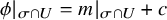
Definition A (Tropicalization).
Let X be a toroidal embedding with no self-intersections. The tropicalization of X in the category of tropical spaces is obtained by endowing the boundary (extended) cone complex
 $\overline {\Sigma }_X$
with the sheaf of affine functions from Definition 3.1.
$\overline {\Sigma }_X$
with the sheaf of affine functions from Definition 3.1.
Informally, if
 $\sigma \in \Sigma _X$
corresponds to a (closed) stratum
$\sigma \in \Sigma _X$
corresponds to a (closed) stratum
 $V(\sigma )\subseteq X$
, a piecewise linear function
$V(\sigma )\subseteq X$
, a piecewise linear function
 $\phi $
defined on a neighborhood
$\phi $
defined on a neighborhood
 $\Sigma _X^\sigma $
of
$\Sigma _X^\sigma $
of
 $\sigma $
is declared affine when the corresponding line bundle (defined on the open set
$\sigma $
is declared affine when the corresponding line bundle (defined on the open set
 $X_\sigma $
obtained by removing all boundary divisors that do not meet
$X_\sigma $
obtained by removing all boundary divisors that do not meet
 $V(\sigma )$
) trivializes on
$V(\sigma )$
) trivializes on
 $V(\sigma )$
:
$V(\sigma )$
:
 $$ \begin{align} {\mathcal O}_{X_\sigma}(\phi)\vert_{ V(\sigma)}\cong {\mathcal O}_{V(\sigma)}. \end{align} $$
When
 $\sigma /\tau $
is a cone at infinity, one makes the additional requirement that
$\sigma /\tau $
is a cone at infinity, one makes the additional requirement that
 $\phi $
is constant on
$\phi $
is constant on
 $\tau $
, meaning that the support of the divisor associated to
$\tau $
, meaning that the support of the divisor associated to
 $\phi $
does not contain any boundary divisor containing
$\phi $
does not contain any boundary divisor containing
 $V(\tau )$
. This notion of tropicalization is functorial, and it is invariant under log modifications of the toroidal variety X.
$V(\tau )$
. This notion of tropicalization is functorial, and it is invariant under log modifications of the toroidal variety X.
Theorem B (Proposition 3.5, Proposition 3.8).
A morphism of toroidal varieties
 $f: X\to Y$
induces a morphism of tropical spaces:
$f: X\to Y$
induces a morphism of tropical spaces:
 $$ \begin{align} F:= {\mathtt{Trop}}(f) \colon \vert \Sigma_X\vert\to \vert \Sigma_Y\vert . \end{align} $$
If f is a log modification, then F is an isomorphism.
Since the main application of this technology is to families of curves, an important check of the soundness of the definitions is that in genus zero this notion of tropicalization recovers the previous ones (via torus embedding [Reference Maclagan and Sturmfels20] or cross ratios [Reference Cavalieri, Gross and Markwig6]).
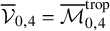
Theorem C (Theorem 3.17).
The tropicalization of the toroidal variety
 $\overline {\mathcal M}_{0,n}$
is the tropical space
$\overline {\mathcal M}_{0,n}$
is the tropical space
 ${\mathcal M}_{0,n}^{\mathtt {trop}}$
.
${\mathcal M}_{0,n}^{\mathtt {trop}}$
.
The situation is more subtle for curves of positive genus. A family
 $\pi : \mathcal C\to \mathcal B$
of logarithmic curves naturally produces a map of extended cone complexes
$\pi : \mathcal C\to \mathcal B$
of logarithmic curves naturally produces a map of extended cone complexes
 $\Pi : {\overline { \mathtt C}}\to {\overline { \mathtt B}}$
; we call the family tropicalizable if its tropicalization gives rise to the expected (set theoretic) moduli map. As soon as a family of curves is tropicalizable, it is almost a family of tropical curves in the sense of [Reference Cavalieri, Gross and Markwig6, Definition 3.10].
$\Pi : {\overline { \mathtt C}}\to {\overline { \mathtt B}}$
; we call the family tropicalizable if its tropicalization gives rise to the expected (set theoretic) moduli map. As soon as a family of curves is tropicalizable, it is almost a family of tropical curves in the sense of [Reference Cavalieri, Gross and Markwig6, Definition 3.10].
Theorem D (Proposition 3.21, Proposition 3.22).
Given
 $\pi : \mathcal C\to \mathcal B$
a tropicalizable family of stable, n-marked logarithmic curves, we obtain a map of tropical spaces
$\pi : \mathcal C\to \mathcal B$
a tropicalizable family of stable, n-marked logarithmic curves, we obtain a map of tropical spaces
 $\Pi : {\overline { \mathtt C}}\to {\overline { \mathtt B}}$
such that:
$\Pi : {\overline { \mathtt C}}\to {\overline { \mathtt B}}$
such that:
-
• if x is a genus-
 $0$
point of
${\overline { \mathtt C}}$
, we have the exact sequence (1.3)
$$ \begin{align} 0 \to \operatorname{\mathrm{Aff}}_{\overline{ \mathtt B},{\Pi }(x)}\to \operatorname{\mathrm{Aff}}_{{\overline{ \mathtt C}},x} \to \Omega^1_{{{\overline{ \mathtt C}}}_{{\Pi }(x)},x}\to 0 . \end{align} $$
$0$
point of
${\overline { \mathtt C}}$
, we have the exact sequence (1.3)
$$ \begin{align} 0 \to \operatorname{\mathrm{Aff}}_{\overline{ \mathtt B},{\Pi }(x)}\to \operatorname{\mathrm{Aff}}_{{\overline{ \mathtt C}},x} \to \Omega^1_{{{\overline{ \mathtt C}}}_{{\Pi }(x)},x}\to 0 . \end{align} $$
-
• if x is a rational vertex of
${\overline { \mathtt C}}$
or a point on an edge adjacent to a rational vertex, then, near x, the affine functions on its fiber consist of all harmonic functions.


A necessary step towards tropicalizing
 $\psi $
classes is to define the notion of tropicalization of line bundles. In the next result we discuss when such an object is a tropical line bundle.
$\psi $
classes is to define the notion of tropicalization of line bundles. In the next result we discuss when such an object is a tropical line bundle.
Theorem E (Proposition 4.4, Proposition 4.6).
Denote by
 $\mathcal L$
the invertible sheaf of a line bundle
$\mathcal L$
the invertible sheaf of a line bundle
 $L\to X$
; let
$L\to X$
; let
 ${\mathtt {Trop}}(L)$
be the tropicalization of the total space of L and
${\mathtt {Trop}}(L)$
be the tropicalization of the total space of L and
 $\mathtt {U} \subseteq \overline {\Sigma }_X$
an open subcomplex of the tropicalization of the base space.
$\mathtt {U} \subseteq \overline {\Sigma }_X$
an open subcomplex of the tropicalization of the base space.
-
1.
${\mathtt {Trop}}(L)$
is a tropical line bundle on
$\mathtt U$
if and only if for every
$\sigma /\tau \in U$
there exists a strictly piecewise linear function
$\phi _{\sigma /\tau }$
on a neighborhood of
$\tau $
that is constant on
$\tau $
such that (1.4)
$$ \begin{align} \left(\mathcal O_{X_{\sigma}}(\phi_{\sigma/\tau}) \otimes \mathcal L\right)\vert_{V(\sigma)} \cong \mathcal O_{V(\sigma)} . \end{align} $$
-
2. if
$\mathcal L = \mathcal O_X(\phi )$
, for
$\phi $
a strict piecewise linear function on
$\Sigma _X$
, then condition (1.4) is equivalent to the existence of an affine function
$\chi _{\sigma /\tau }$
on a neighborhood of
$\sigma $
such that (1.5)
$$ \begin{align} \chi\vert_{\tau} = \phi\vert_{\tau}. \end{align} $$


With this technology in place, we turn our attention to the i-th cotangent line bundle of a family of curves
 $\mathcal C\to \mathcal B$
. The main result is that if the tropicalization
$\mathcal C\to \mathcal B$
. The main result is that if the tropicalization
 $\overline {{ \mathtt C}}\to \overline { \mathtt B}$
has enough local affine functions near the i-th section at infinity, then the tropicalization of the cotangent line bundle agrees with the definition of the tropical cotangent line bundle from [Reference Cavalieri, Gross and Markwig6, Definition 6.16].
$\overline {{ \mathtt C}}\to \overline { \mathtt B}$
has enough local affine functions near the i-th section at infinity, then the tropicalization of the cotangent line bundle agrees with the definition of the tropical cotangent line bundle from [Reference Cavalieri, Gross and Markwig6, Definition 6.16].
Theorem F (Theorem 5.5, Corollary 5.11).
Let
 $\mathcal C \to \mathcal B$
be a family of n-marked stable curves with tropicalization
$\mathcal C \to \mathcal B$
be a family of n-marked stable curves with tropicalization
 $\overline {{ \mathtt C}}\to \overline { \mathtt B}$
, and let
$\overline {{ \mathtt C}}\to \overline { \mathtt B}$
, and let
 $\phi _i$
be the strict piecewise linear function on
$\phi _i$
be the strict piecewise linear function on
 ${ \mathtt C}$
having slope one along the ray dual to the i-th section of the family, and
${ \mathtt C}$
having slope one along the ray dual to the i-th section of the family, and
 $0$
on all other rays. If
$0$
on all other rays. If
 $\operatorname {\mathrm {Aff}}_{\overline {{ \mathtt C}}}(\phi _i)$
is a tropical line bundle, then
$\operatorname {\mathrm {Aff}}_{\overline {{ \mathtt C}}}(\phi _i)$
is a tropical line bundle, then
By taking first Chern classes, we obtain
 $$ \begin{align} {\mathtt{Trop}}(\psi_i)= \psi_i^{\mathtt{trop}} . \end{align} $$
In genus greater than
 $1$
, the
$1$
, the
 $\psi $
classes are not boundary classes, but supported on the interior
$\psi $
classes are not boundary classes, but supported on the interior
 $\mathcal M_{g,n}$
. Tropical geometry usually only captures information about the boundary. So Theorem 5.5 can be paraphrased in elementary terms as follows: if we are able to sufficiently degenerate a family of curves such that it becomes tropicalizable, a condition which can be checked easily in applications, tropical geometry captures all numerical information about the
$\mathcal M_{g,n}$
. Tropical geometry usually only captures information about the boundary. So Theorem 5.5 can be paraphrased in elementary terms as follows: if we are able to sufficiently degenerate a family of curves such that it becomes tropicalizable, a condition which can be checked easily in applications, tropical geometry captures all numerical information about the
 $\psi $
classes, even though they are not boundary.
$\psi $
classes, even though they are not boundary.
We conclude the manuscript with an extended example. We compute the tropical
 $\psi $
classes for two two-dimensional families of genus-one, tropical curves, obtained by stabilization from a space of tropical admissible covers. We show that the tropical
$\psi $
classes for two two-dimensional families of genus-one, tropical curves, obtained by stabilization from a space of tropical admissible covers. We show that the tropical
 $\psi $
classes of [Reference Cavalieri, Gross and Markwig6] are the tropicalization of the algebraic
$\psi $
classes of [Reference Cavalieri, Gross and Markwig6] are the tropicalization of the algebraic
 $\psi $
classes, and that they agree with the operational perspective of tropicalization from [Reference Katz17].
$\psi $
classes, and that they agree with the operational perspective of tropicalization from [Reference Katz17].
1.2 Context and commentary
Tropical geometry and moduli spaces of curves have enjoyed fruitful interactions ever since Mikhalkin’s seminal paper [Reference Mikhalkin21] interpreted the space of phylogenetic trees of [Reference Billera, Holmes and Vogtmann2] as the tropicalization of
 $\mathcal M_{0,n}$
. With Hannah Markwig, we gave our perspective and account on the evolution of the subject in the introduction to [Reference Cavalieri, Gross and Markwig6], to which we refer the interested reader. The one line (cheeky) summary is, when it comes to tropical geometry and moduli spaces of curves, anything you may wish comes true for rational curves, while it appears to crash and burn for positive genus. This article is part of a collection of works (including, but not limited to [Reference Abramovich, Caporaso and Payne1, Reference Cavalieri, Chan, Ulirsch and Wise5, Reference Chan, Galatius and Payne8, Reference Cavalieri, Gross and Markwig6]) arguing that tropical geometry can still provide a meaningful and powerful approach to the study of the geometry and intersection theory of moduli spaces of positive genus curves.
$\mathcal M_{0,n}$
. With Hannah Markwig, we gave our perspective and account on the evolution of the subject in the introduction to [Reference Cavalieri, Gross and Markwig6], to which we refer the interested reader. The one line (cheeky) summary is, when it comes to tropical geometry and moduli spaces of curves, anything you may wish comes true for rational curves, while it appears to crash and burn for positive genus. This article is part of a collection of works (including, but not limited to [Reference Abramovich, Caporaso and Payne1, Reference Cavalieri, Chan, Ulirsch and Wise5, Reference Chan, Galatius and Payne8, Reference Cavalieri, Gross and Markwig6]) arguing that tropical geometry can still provide a meaningful and powerful approach to the study of the geometry and intersection theory of moduli spaces of positive genus curves.
The notion of tropical
 $\psi $
classes for families of tropical curves of arbitrary genus was introduced in [Reference Cavalieri, Gross and Markwig6]. The key step there was to define the notion of family of tropical curves by requiring an affine structure, that is, distinguished subsheaves of the sheaves of piecewise linear functions on both the base and the total space of the family satisfying some natural requirements: for example that the restriction of affine functions to fibers are harmonic (see Section 2.1 for a more complete review). Borrowing intuition from the algebraic identification of the
$\psi $
classes for families of tropical curves of arbitrary genus was introduced in [Reference Cavalieri, Gross and Markwig6]. The key step there was to define the notion of family of tropical curves by requiring an affine structure, that is, distinguished subsheaves of the sheaves of piecewise linear functions on both the base and the total space of the family satisfying some natural requirements: for example that the restriction of affine functions to fibers are harmonic (see Section 2.1 for a more complete review). Borrowing intuition from the algebraic identification of the
 $\psi $
class with the negative self-intersection of the corresponding section, the tropical cotangent line bundle
$\psi $
class with the negative self-intersection of the corresponding section, the tropical cotangent line bundle ![]() of a family of tropical curves
of a family of tropical curves
 $\overline {{ \mathtt C}}\to \overline { \mathtt B}$
is defined to be the pullback via the i-th section of the tropical counterpart of the co-normal bundle to the section: the
$\overline {{ \mathtt C}}\to \overline { \mathtt B}$
is defined to be the pullback via the i-th section of the tropical counterpart of the co-normal bundle to the section: the
 $\operatorname {\mathrm {Aff}}_{{ \mathtt C}}$
torsor whose local sections are affine functions on the finite part of
$\operatorname {\mathrm {Aff}}_{{ \mathtt C}}$
torsor whose local sections are affine functions on the finite part of
 $\overline {{ \mathtt C}}$
, going to infinity towards the section
$\overline {{ \mathtt C}}$
, going to infinity towards the section
 ${\mathtt s}_i$
with slope
${\mathtt s}_i$
with slope
 $1$
along the fibers of the family.
$1$
along the fibers of the family.
The theory thus obtained is a combinatorial theory where the affine structures are canonically determined in certain cases: for example, for families of explicit tropical curves (that is when all vertices are rational); in this case we have natural correspondence statements with the corresponding algebraic families. In general, the theory of tropical
 $\psi $
classes is strictly broader than the algebraic one: in [Reference Cavalieri, Gross and Markwig6, Example 6.17], the authors exhibited one-dimensional families of tropical curves where the degree of the tropical
$\psi $
classes is strictly broader than the algebraic one: in [Reference Cavalieri, Gross and Markwig6, Example 6.17], the authors exhibited one-dimensional families of tropical curves where the degree of the tropical
 $\psi $
class cannot agree with the degree of
$\psi $
class cannot agree with the degree of
 $\psi $
on any corresponding algebraic family.
$\psi $
on any corresponding algebraic family.
In order to make a meaningful connection with algebraic geometry, we define a notion of tropicalization which is less restrictive than torus embedded tropicalization, yet still contains information about affine structures. While ultimately we wish to apply our constructions to logarithmic families of log smooth curves, we choose to develop the main definitions in the simpler set-up and language of toroidal embeddings with no self-intersections (which we call toroidal varieties for simplicity): varieties with a distinguished divisor called boundary, which are locally isomorphic to toric varieties. A toroidal variety is assigned, in a functorial way, a cone complex agreeing with the (cone over the topological) boundary complex, where each cone is additionally endowed with an integral lattice, see [Reference Kempf, Faye Knudsen, Mumford and Saint-Donat18].
In order to define a natural notion of affine structure on the cone complex of a toroidal variety, we use the following intuition from toric varieties and tropicalization of subvarieties of tori: piecewise linear functions on the fan of a toric variety correspond to Cartier divisors, and therefore line bundles; the main role of the torus in these theories is that its characters are a class of functions that are invertible in the interior of the space, which can be thought of as sections of bundles that trivialize in the interior. We thus choose to define a piecewise linear function on (an open set of) the cone complex of a toroidal variety to be affine when the corresponding line bundle trivializes (on some collection of orbits depending on the chosen open set)Footnote 1. The resulting affine structure makes the cone complex into a tropical space, which we call the tropicalization of the toroidal variety.
In the broader generality of logarithmic schemes with a divisorial log structure, a functorial assignment of a generalized cone complex is given in [Reference Ulirsch25], where it is called logarithmic tropicalization; the fact that multiple faces of a single cone can be identified makes it a bit delicate to immediately define an affine structure on the logarithmic tropicalization. We circumvent this problem by observing that the sheaf of affine functions defined is invariant under logarithmic modifications (roughly speaking sequences of blow-ups and blow-downs of strata and their transforms); a generalized cone complex can be refined to an honest cone complex, which is the cone complex of an appropriate log modification of the original space. Hence one may define the affine structure on the logarithmic tropicalization via any suitable log modification making the space toroidal.
There are two classes of objects whose tropicalization we are especially interested in: families of curves and line bundles. We begin discussing the latter.
Besides special cases like toric varieties, Mumford curves, or totally degenerating Abelian varieties, there is no known procedure to tropicalize (algebraic) line bundles to tropical line bundles in the sense of [Reference Mikhalkin and Zharkov22, Definition 4.4](see Section 2.4). Of course, there is a naïve approach: a line bundle L over a toroidal variety X may be given a natural toroidal boundary, obtained as the union of the pull-back of the boundary on the base, plus the zero section. We define the (naïve) tropicalization of L essentially to be the tropicalization of its total space, see Remark 4.2. The result is a tropical space, but it may not have enough affine functions to actually be a tropical line bundle. We find that there is a concise condition for the tropicalization of L to be a tropical line bundle on an open neighborhood of a cone
 $\sigma \in \Sigma _X$
: it amounts to the invertible sheaf
$\sigma \in \Sigma _X$
: it amounts to the invertible sheaf
 $\mathcal L$
of L restricted to the orbit
$\mathcal L$
of L restricted to the orbit
 $V(\sigma )$
being the restriction of a sheaf of boundary type, i.e.,
$V(\sigma )$
being the restriction of a sheaf of boundary type, i.e.,
 $$ \begin{align} \mathcal L\vert_{ V(\sigma)} \cong \mathcal O_{X_\sigma}\left(\sum a_\rho D_\rho\right)\big\vert_{ V(\sigma)}, \end{align} $$
where the
 $D_\rho $
’s are the boundary divisors in
$D_\rho $
’s are the boundary divisors in
 $X_\sigma $
. For a cone at infinity
$X_\sigma $
. For a cone at infinity
 $\sigma /\tau $
the situation is analogous: we need
$\sigma /\tau $
the situation is analogous: we need
 $\mathcal L\vert _{ V(\sigma )}$
to be of the form
$\mathcal L\vert _{ V(\sigma )}$
to be of the form
 $\mathcal O_{ V(\tau )_\sigma }(\sum a_\rho (D_\rho \cap V(\tau )))\vert _{V(\sigma )}$
, where the
$\mathcal O_{ V(\tau )_\sigma }(\sum a_\rho (D_\rho \cap V(\tau )))\vert _{V(\sigma )}$
, where the
 $D_\rho $
’s are boundary divisors which do not contain the orbit
$D_\rho $
’s are boundary divisors which do not contain the orbit
 $V(\tau )$
: this means that on
$V(\tau )$
: this means that on
 $V(\sigma )$
, the line bundle is the restriction of a line bundle of boundary type on the orbit
$V(\sigma )$
, the line bundle is the restriction of a line bundle of boundary type on the orbit
 $V(\tau )$
. It follows that a line bundle of boundary type, which we associate to a piecewise linear function
$V(\tau )$
. It follows that a line bundle of boundary type, which we associate to a piecewise linear function
 $\phi $
on
$\phi $
on
 $\Sigma _X$
, tropicalizes to a tropical line bundle on the cone complex
$\Sigma _X$
, tropicalizes to a tropical line bundle on the cone complex
 $\Sigma _X$
, but not necessarily on the whole extended cone complex
$\Sigma _X$
, but not necessarily on the whole extended cone complex
 $\overline {\Sigma }_X$
. We identify a combinatorial condition, which we call being combinatorially principal, that makes it a tropical line bundle on a cone at infinity of the form
$\overline {\Sigma }_X$
. We identify a combinatorial condition, which we call being combinatorially principal, that makes it a tropical line bundle on a cone at infinity of the form
 $\sigma /\tau $
: there must exist an affine function
$\sigma /\tau $
: there must exist an affine function
 $\phi _\tau $
which agrees with
$\phi _\tau $
which agrees with
 $\phi $
on the cone
$\phi $
on the cone
 $\tau $
.
$\tau $
.
Turning our attention to families of curves, given a family
 $\pi \colon \mathcal C\to \mathcal B$
, the tropicalization gives a map of tropical spaces
$\pi \colon \mathcal C\to \mathcal B$
, the tropicalization gives a map of tropical spaces
 $\Pi \colon \overline {{ \mathtt C}}\to \overline {{ \mathtt B}}$
. A paraphrase of
$\Pi \colon \overline {{ \mathtt C}}\to \overline {{ \mathtt B}}$
. A paraphrase of
 $\mathcal C\to \mathcal B$
being tropicalizable is that, once appropriately endowing the points of
$\mathcal C\to \mathcal B$
being tropicalizable is that, once appropriately endowing the points of
 $\overline {{ \mathtt C}}$
with a genus function, the fibers of
$\overline {{ \mathtt C}}$
with a genus function, the fibers of
 $\Pi $
are the dual graphs of the corresponding fibers of
$\Pi $
are the dual graphs of the corresponding fibers of
 $\pi $
. This is some sort of minimal requirement, that due to automorphisms and monodromy issues may not always be guaranteed: in Example 3.20 we see an instance of what may go wrong and how it can be remedied.
$\pi $
. This is some sort of minimal requirement, that due to automorphisms and monodromy issues may not always be guaranteed: in Example 3.20 we see an instance of what may go wrong and how it can be remedied.
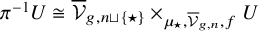
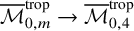
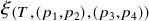
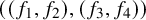
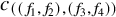
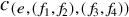
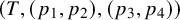
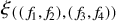
By functoriality, tropical cross ratios are tropicalizations of algebraic cross ratios, see Figure 1. This fact guarantees that this notion of tropicalization agrees with the classical notion (coming from embedding into a torus) for families of rational pointed curves and gives yet another equivalent way to get to
 $\mathcal M_{0,n}^{\mathtt {trop}}$
. The tropicalization
$\mathcal M_{0,n}^{\mathtt {trop}}$
. The tropicalization
 $\overline {{ \mathtt C}}\to \overline {{ \mathtt B}}$
is in general not a family of tropical curves in the sense of [Reference Cavalieri, Gross and Markwig6, Definition 3.10]: one may not have enough (germs of) affine functions on the fibers, but this failure is restricted to points of positive genus, or points on edges that are not adjacent to any rational vertex. In particular, we recover the result from [Reference Cavalieri, Gross and Markwig6, Proposition 4.24] that
$\overline {{ \mathtt C}}\to \overline {{ \mathtt B}}$
is in general not a family of tropical curves in the sense of [Reference Cavalieri, Gross and Markwig6, Definition 3.10]: one may not have enough (germs of) affine functions on the fibers, but this failure is restricted to points of positive genus, or points on edges that are not adjacent to any rational vertex. In particular, we recover the result from [Reference Cavalieri, Gross and Markwig6, Proposition 4.24] that
 $\overline {{ \mathtt C}}\to \overline {{ \mathtt B}}$
is a family of tropical curves when the image of
$\overline {{ \mathtt C}}\to \overline {{ \mathtt B}}$
is a family of tropical curves when the image of
 ${{ \mathtt B}}$
via the tropical moduli map lies in the good locus
${{ \mathtt B}}$
via the tropical moduli map lies in the good locus
 ${\mathcal V^{\mathrm {good}}_{g,n}}$
([Reference Cavalieri, Gross and Markwig6, Definition 4.22]).
${\mathcal V^{\mathrm {good}}_{g,n}}$
([Reference Cavalieri, Gross and Markwig6, Definition 4.22]).
An illustration that tropical cross ratios are the tropicalization of algebraic cross ratios. The top of the figure shows a cross ratio as factoring through a morphism to
 $\overline {\mathcal M}_{0,4}$
, which is then identified with
$\overline {\mathcal M}_{0,4}$
, which is then identified with ![]() (the difference between the two spaces is the boundary structure). Tropical cross ratios are similarly obtained in the row below. Functoriality of tropicalization shows the bottom part of the figure to be the tropicalization of the top.
(the difference between the two spaces is the boundary structure). Tropical cross ratios are similarly obtained in the row below. Functoriality of tropicalization shows the bottom part of the figure to be the tropicalization of the top.

For a family of marked tropical curves
 $\overline {{ \mathtt C}}\to \overline {{ \mathtt B}}$
, the tropical cotangent line bundle to the i-th section is defined as
$\overline {{ \mathtt C}}\to \overline {{ \mathtt B}}$
, the tropical cotangent line bundle to the i-th section is defined as
see [Reference Cavalieri, Gross and Markwig6, Definition 6.16]. In this paper, we define
 $\operatorname {\mathrm {Aff}}_{\overline {{ \mathtt C}}}(-{\mathtt s}_i)$
when
$\operatorname {\mathrm {Aff}}_{\overline {{ \mathtt C}}}(-{\mathtt s}_i)$
when
 $\overline {{ \mathtt C}}$
is a tropical space, and observe that in general it is a pseudo
$\overline {{ \mathtt C}}$
is a tropical space, and observe that in general it is a pseudo
 $\operatorname {\mathrm {Aff}}_{\overline {{ \mathtt C}}}$
torsor: its local sections either give a torsor or are empty. An important observation from [Reference Cavalieri, Gross and Markwig6, Propositions 3.24, 3.25] is that
$\operatorname {\mathrm {Aff}}_{\overline {{ \mathtt C}}}$
torsor: its local sections either give a torsor or are empty. An important observation from [Reference Cavalieri, Gross and Markwig6, Propositions 3.24, 3.25] is that
 $\overline { \mathtt C}\to \overline { \mathtt B}$
being a family of tropical curves ensures that
$\overline { \mathtt C}\to \overline { \mathtt B}$
being a family of tropical curves ensures that
 $\operatorname {\mathrm {Aff}}_{\overline { \mathtt C}}(-{\mathtt s}_i)$
really is an
$\operatorname {\mathrm {Aff}}_{\overline { \mathtt C}}(-{\mathtt s}_i)$
really is an
 $\operatorname {\mathrm {Aff}}_{\overline { \mathtt C}}$
-torsor. However, this condition is stronger than strictly necessary: for
$\operatorname {\mathrm {Aff}}_{\overline { \mathtt C}}$
-torsor. However, this condition is stronger than strictly necessary: for
 $\operatorname {\mathrm {Aff}}_{\overline { \mathtt C}}(-{\mathtt s}_i)$
to be a tropical line bundle, the affine structure of
$\operatorname {\mathrm {Aff}}_{\overline { \mathtt C}}(-{\mathtt s}_i)$
to be a tropical line bundle, the affine structure of
 $\overline {{ \mathtt C}}$
only matters locally near
$\overline {{ \mathtt C}}$
only matters locally near
 ${\mathtt s}_i$
, so one only needs
${\mathtt s}_i$
, so one only needs
 $\overline {{ \mathtt C}}\to \overline {{ \mathtt B}}$
to satisfy the conditions on the affine structure of families of tropical curves in a neighborhood of
$\overline {{ \mathtt C}}\to \overline {{ \mathtt B}}$
to satisfy the conditions on the affine structure of families of tropical curves in a neighborhood of
 ${\mathtt s}_i(\overline { \mathtt B})$
. When this happens, it is then possible to check that the tropicalization of the cotangent line bundle is a tropical line bundle, and it agrees with
${\mathtt s}_i(\overline { \mathtt B})$
. When this happens, it is then possible to check that the tropicalization of the cotangent line bundle is a tropical line bundle, and it agrees with
 ${\mathtt s}_i^\ast (\operatorname {\mathrm {Aff}}_{\overline { \mathtt C}}(-{\mathtt s}_i))$
.
${\mathtt s}_i^\ast (\operatorname {\mathrm {Aff}}_{\overline { \mathtt C}}(-{\mathtt s}_i))$
.
Pulling all the loose strings together, one finally can answer the motivating question we began this section with.
Given a tropicalizable family of stable marked curves
 $\mathcal C \to \mathcal B $
with tropicalization
$\mathcal C \to \mathcal B $
with tropicalization
 $\overline {{ \mathtt C}}\to \overline {{ \mathtt B}}$
, we have
$\overline {{ \mathtt C}}\to \overline {{ \mathtt B}}$
, we have
 $$ \begin{align} {\mathtt{Trop}}(\psi_i)= \psi_i^{\mathtt{trop}} \end{align} $$
whenever
 $\operatorname {\mathrm {Aff}}_{\overline { \mathtt C}}(-{\mathtt s}_i)$
is a tropical line bundle; further, this notion admits the following combinatorial characterization: the piecewise linear function
$\operatorname {\mathrm {Aff}}_{\overline { \mathtt C}}(-{\mathtt s}_i)$
is a tropical line bundle; further, this notion admits the following combinatorial characterization: the piecewise linear function
 $\phi _{\rho _i}$
on
$\phi _{\rho _i}$
on
 $\overline { \mathtt C}$
having slope one on the ray
$\overline { \mathtt C}$
having slope one on the ray
 $\rho _i$
dual to
$\rho _i$
dual to
 $s_i$
and zero on all other rays is combinatorially principal.
$s_i$
and zero on all other rays is combinatorially principal.
One might interpret the above conclusion as follows: tropical geometry does not see the algebraic information contained in
 $\psi $
classes on all families of curves. In order to capture this information tropically, the family must degenerate sufficiently near the section. However, when tropical geometry does see
$\psi $
classes on all families of curves. In order to capture this information tropically, the family must degenerate sufficiently near the section. However, when tropical geometry does see
 $\psi $
classes, it indeed sees the tropical
$\psi $
classes, it indeed sees the tropical
 $\psi $
classes of [Reference Cavalieri, Gross and Markwig6].
$\psi $
classes of [Reference Cavalieri, Gross and Markwig6].
1.3 Computations
We conclude this paper with an extended example of a computation of tropical
 $\psi $
classes for two two-dimensional families of tropical curves of genus
$\psi $
classes for two two-dimensional families of tropical curves of genus
 $1$
with two marked points. The families are obtained from tropical admissible covers by forgetting some of the marked ends. In both cases we show that the tropical
$1$
with two marked points. The families are obtained from tropical admissible covers by forgetting some of the marked ends. In both cases we show that the tropical
 $\psi $
class is the tropicalization of the algebraic
$\psi $
class is the tropicalization of the algebraic
 $\psi $
class, and exhibit it as a one-dimensional tropical cycle, that is a Minkowski weight on the base of the family. The tropical cycle obtained agrees with the operational tropicalization of the
$\psi $
class, and exhibit it as a one-dimensional tropical cycle, that is a Minkowski weight on the base of the family. The tropical cycle obtained agrees with the operational tropicalization of the
 $\psi $
class, that is with the Minkowski weight decorating each cone with the intersection number of
$\psi $
class, that is with the Minkowski weight decorating each cone with the intersection number of
 $\psi $
with the corresponding stratum. Besides illustrating a concrete instance of the theoretical story told, there are some interesting lessons one can observe from this extended example. In order to prove that the tropicalization of the families curves have enough affine functions to define the tropical
$\psi $
with the corresponding stratum. Besides illustrating a concrete instance of the theoretical story told, there are some interesting lessons one can observe from this extended example. In order to prove that the tropicalization of the families curves have enough affine functions to define the tropical
 $\psi $
classes it is more efficient to rely on functoriality, rather than on the direct definition of tropicalization. Then one is essentially able to use the affine functions from the genus zero theory to obtain affine functions near the section. The second observation is that the combinatorics of tropical intersection theory is manageable, which is encouraging that this technology might prove a useful tool for the study of tautological rings of moduli spaces of curves. There has been recent interest in approaching the study of the logarithmic tautological ring of moduli spaces of curves [Reference Holmes and Schwarz13, Reference Molcho, Pandharipande and Schmitt23, Reference Molcho and Ranganathan24] as the image of a ring homomorphism from the ring of piecewise polynomial functions on
$\psi $
classes it is more efficient to rely on functoriality, rather than on the direct definition of tropicalization. Then one is essentially able to use the affine functions from the genus zero theory to obtain affine functions near the section. The second observation is that the combinatorics of tropical intersection theory is manageable, which is encouraging that this technology might prove a useful tool for the study of tautological rings of moduli spaces of curves. There has been recent interest in approaching the study of the logarithmic tautological ring of moduli spaces of curves [Reference Holmes and Schwarz13, Reference Molcho, Pandharipande and Schmitt23, Reference Molcho and Ranganathan24] as the image of a ring homomorphism from the ring of piecewise polynomial functions on
 $\mathcal M_{g,n}^{\mathtt {trop}}$
. The affine linear functions defined here generate an ideal that lies in the kernel of that ring homomorphism.
$\mathcal M_{g,n}^{\mathtt {trop}}$
. The affine linear functions defined here generate an ideal that lies in the kernel of that ring homomorphism.
1.4 Notations and Conventions
We assume throughout working on an algebraically closed field of characteristic
 $0$
; we expect all constructions to go through for perfect fields, but care should be taken to what objects the constructions are applied to. In this paper, the tropical semiring is
$0$
; we expect all constructions to go through for perfect fields, but care should be taken to what objects the constructions are applied to. In this paper, the tropical semiring is ![]() ; the choice of this convention is to make the affine structure near the section at infinity parallel the affine structure of the tropicalization of the normal bundle to the section near its “zero” section. We mostly use calligraphic fonts for algebraic objects, and typewriter ones for tropical objects. The superscript
; the choice of this convention is to make the affine structure near the section at infinity parallel the affine structure of the tropicalization of the normal bundle to the section near its “zero” section. We mostly use calligraphic fonts for algebraic objects, and typewriter ones for tropical objects. The superscript
 ${\mathtt {trop}}$
is used for certain tropical objects where the use of an identifying font was considered not viable, whereas the tropicalization functor is denoted by
${\mathtt {trop}}$
is used for certain tropical objects where the use of an identifying font was considered not viable, whereas the tropicalization functor is denoted by
 ${\mathtt {Trop}}$
.
${\mathtt {Trop}}$
.
2 Preliminaries
We recall the relevant definitions and results about tropical moduli spaces of curves, tropical cycles, and tropical line bundles in the generality introduced in [Reference Cavalieri, Gross and Markwig6]. We refer to that manuscript for a comprehensive list of references to the relevant preexisting literature.
2.1 Tropical curves and their moduli
In [Reference Cavalieri, Gross and Markwig6], moduli spaces of tropical curves are introduced as stacks over the category of tropical spaces. We review the relevant definitions.
A TPL-space is a pair
 $({ X}, {\mathrm {PL}}_{ X})$
consisting of a topological space
$({ X}, {\mathrm {PL}}_{ X})$
consisting of a topological space
 ${ X}$
and a sheaf
${ X}$
and a sheaf
 ${\mathrm {PL}}_{X}$
of continuous
${\mathrm {PL}}_{X}$
of continuous ![]() -valued functions on
-valued functions on
 ${ X}$
that is locally isomorphic to
${ X}$
that is locally isomorphic to
 $(U, {\mathrm {PL}}_U)$
, the sheaf of continuous, integral, piecewise linear functions of some open subset U of a rational polyhedral set P in
$(U, {\mathrm {PL}}_U)$
, the sheaf of continuous, integral, piecewise linear functions of some open subset U of a rational polyhedral set P in ![]() . Here, two pairs
. Here, two pairs
 $(Y, \mathcal F_Y)$
and
$(Y, \mathcal F_Y)$
and
 $(Z, \mathcal F_Z)$
of topological spaces and sheaves of functions on them are isomorphic if there exists a homeomorphism
$(Z, \mathcal F_Z)$
of topological spaces and sheaves of functions on them are isomorphic if there exists a homeomorphism
 $f\colon Y\to Z$
so that for a function
$f\colon Y\to Z$
so that for a function
 $\phi $
on an open subset of Z we have that
$\phi $
on an open subset of Z we have that
 $\phi \circ f$
is a section of
$\phi \circ f$
is a section of
 $\mathcal F_Y$
if and only if
$\mathcal F_Y$
if and only if
 $\phi $
is a section of
$\phi $
is a section of
 $\mathcal F_Z$
. For a TPL-space
$\mathcal F_Z$
. For a TPL-space
 ${ X}$
we denote by
${ X}$
we denote by
 ${\mathrm {PL}}^{\mathrm {fin}}_{ X}$
the subsheaf of
${\mathrm {PL}}^{\mathrm {fin}}_{ X}$
the subsheaf of ![]() -valued piecewise linear functions. A morphism of TPL-spaces is a continuous map that pulls piecewise linear functions (section of
-valued piecewise linear functions. A morphism of TPL-spaces is a continuous map that pulls piecewise linear functions (section of
 ${\mathrm {PL}}$
) back to piecewise linear functions.
${\mathrm {PL}}$
) back to piecewise linear functions.
A tropical space is a pair
 $(\mathtt {X}, \operatorname {\mathrm {Aff}}_{\mathtt X})$
consisting of a TPL-space
$(\mathtt {X}, \operatorname {\mathrm {Aff}}_{\mathtt X})$
consisting of a TPL-space
 ${\mathtt X}$
and a subsheaf
${\mathtt X}$
and a subsheaf
 $\operatorname {\mathrm {Aff}}_{\mathtt X}\subseteq {\mathrm {PL}}^{\mathrm {fin}}_{\mathtt X}$
, the sheaf of affine functions, that contains the constant sheaf
$\operatorname {\mathrm {Aff}}_{\mathtt X}\subseteq {\mathrm {PL}}^{\mathrm {fin}}_{\mathtt X}$
, the sheaf of affine functions, that contains the constant sheaf ![]() . A morphism of tropical spaces is morphism of TPL-spaces that pulls affine functions back to affine functions. In that case, we also say that the underlying morphism of TPL-spaces is linear. The tropical cotangent bundle is the quotient sheaf
. A morphism of tropical spaces is morphism of TPL-spaces that pulls affine functions back to affine functions. In that case, we also say that the underlying morphism of TPL-spaces is linear. The tropical cotangent bundle is the quotient sheaf ![]() .
.
A tropical curve is a one-dimensional tropical space
 ${ \mathtt C}$
, together with a finitely supported genus function
${ \mathtt C}$
, together with a finitely supported genus function ![]() . The genus of a tropical curve is
. The genus of a tropical curve is
 $\sum _{x\in { \mathtt C}} \gamma (x)+ \mathrm {b_1}({ \mathtt C})$
. A cycle rigidification of a genus-g tropical curve
$\sum _{x\in { \mathtt C}} \gamma (x)+ \mathrm {b_1}({ \mathtt C})$
. A cycle rigidification of a genus-g tropical curve
 ${ \mathtt C}$
is a g-tuple of elements spanning
${ \mathtt C}$
is a g-tuple of elements spanning ![]() and such that each element is either
and such that each element is either
 $0$
or coming from a circuit in
$0$
or coming from a circuit in
 ${ \mathtt C}$
. We denote by
${ \mathtt C}$
. We denote by
 ${\overline {\mathcal V}_{g,n}}$
the set of isomorphism classes of cycle-rigidified stableFootnote 2 n-marked tropical curves of genus g. Forgetting the metric structure (that is, only retaining the topological graph and the cycle rigidification, the so-called combinatorial type) stratifies
${\overline {\mathcal V}_{g,n}}$
the set of isomorphism classes of cycle-rigidified stableFootnote 2 n-marked tropical curves of genus g. Forgetting the metric structure (that is, only retaining the topological graph and the cycle rigidification, the so-called combinatorial type) stratifies
 ${\overline {\mathcal V}_{g,n}}$
into locally closed sets that can be naturally identified with open cones. For a combinatorial type
${\overline {\mathcal V}_{g,n}}$
into locally closed sets that can be naturally identified with open cones. For a combinatorial type
 $\Gamma $
we denote by
$\Gamma $
we denote by
 $\sigma _\Gamma ^\diamond $
the corresponding open cone and by
$\sigma _\Gamma ^\diamond $
the corresponding open cone and by
 $\sigma _\Gamma $
its closure. The natural face morphisms among the closed cones gives
$\sigma _\Gamma $
its closure. The natural face morphisms among the closed cones gives
 ${\overline {\mathcal V}_{g,n}}$
the structure of an extended cone complex. Given an
${\overline {\mathcal V}_{g,n}}$
the structure of an extended cone complex. Given an
 $n\sqcup \{\star \}$
-marked curve, one can forget the
$n\sqcup \{\star \}$
-marked curve, one can forget the
 $\star $
-mark and stabilize. As stabilization is a contraction, a cycle rigidification on the original graph induces a cycle rigidification on the stabilized graph. We thus obtain a map
$\star $
-mark and stabilize. As stabilization is a contraction, a cycle rigidification on the original graph induces a cycle rigidification on the stabilized graph. We thus obtain a map
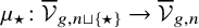
 $$ \begin{align} \mu_\star \colon {\overline {\mathcal V}_{g,n\sqcup\{\star\}}}\to {\overline {\mathcal V}_{g,n}} , \end{align} $$
the forgetful map, which is a morphism of extended cone complexes. The fiber of
 $\mu _\star $
over a point
$\mu _\star $
over a point
 ${\overline {\mathcal V}_{g,n}}$
corresponding to a cycle-rigidified tropical curve
${\overline {\mathcal V}_{g,n}}$
corresponding to a cycle-rigidified tropical curve
 ${ \mathtt C}$
is isomorphic to
${ \mathtt C}$
is isomorphic to
 ${ \mathtt C}$
. In particular, there are n natural sections of
${ \mathtt C}$
. In particular, there are n natural sections of
 $\mu _\star $
and a global genus function
$\mu _\star $
and a global genus function ![]() .
.
A family of genus- g, n-marked stable TPL-curves over a TPL-space
 ${ X}$
is a morphism
${ X}$
is a morphism
 $\pi \colon C\to X$
of TPL-spaces, together with n sections
$\pi \colon C\to X$
of TPL-spaces, together with n sections
 $s_i\colon { X}\to C$
,
$s_i\colon { X}\to C$
,
 $1\leq i\leq n$
, and a genus function
$1\leq i\leq n$
, and a genus function ![]() , such that every
, such that every
 $x\in { X}$
has an open neighborhood U for which there exists a map
$x\in { X}$
has an open neighborhood U for which there exists a map
 $f\colon U\to {\overline {\mathcal V}_{g,n}}$
and an isomorphism
$f\colon U\to {\overline {\mathcal V}_{g,n}}$
and an isomorphism
 $\pi ^{-1}U\cong {\overline {\mathcal V}_{g,n\sqcup \{\star \}}} \times _{\mu _\star ,{\overline {\mathcal V}_{g,n}},f} U$
over U that respects the sections and the genus function.
$\pi ^{-1}U\cong {\overline {\mathcal V}_{g,n\sqcup \{\star \}}} \times _{\mu _\star ,{\overline {\mathcal V}_{g,n}},f} U$
over U that respects the sections and the genus function.
A family of genus- g, n-marked stable tropical curves over a tropical space
 ${\mathtt X}$
is a family of genus-g, n-marked TPL-curves
${\mathtt X}$
is a family of genus-g, n-marked TPL-curves
 $\Pi \colon \mathtt C\to {\mathtt X}$
satisfying the following conditions:
$\Pi \colon \mathtt C\to {\mathtt X}$
satisfying the following conditions:
-
1. for each
$x\in {\mathtt X}$
, the fiber , equipped with the induced affine structure, is a stable tropical curve, -
2. for every
$y\in \mathtt C$
, the sequence (2.2)induced by pull-back from
$$ \begin{align} 0 \to \Omega^1_{{\mathtt X}, \Pi(y)} \to \Omega^1_{{\mathtt C}, y} \to \Omega^1_{{\mathtt C}_{\Pi(y)},y} \to 0 \end{align} $$
${\mathtt X}$
and restriction to
${\mathtt C}_{\Pi (y)}$
, is exact. This can be phrased equivalently as saying that affine functions that are constant on fibers are pull-backs of affine functions on the base.


There is a natural affine structure on the space
 ${\overline {\mathcal V}_{g,n}}$
induced by cross ratio functions. We describe these functions, starting with
${\overline {\mathcal V}_{g,n}}$
induced by cross ratio functions. We describe these functions, starting with
 ${\overline {\mathcal V}_{0,4}}=\overline {\mathcal M}^{\mathrm {trop}}_{0,4}$
. Choosing an ordering, for example,
${\overline {\mathcal V}_{0,4}}=\overline {\mathcal M}^{\mathrm {trop}}_{0,4}$
. Choosing an ordering, for example,
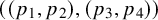 $((p_1,p_2), (p_3,p_4))$
, of the four markings defines two unique minimal paths in a curve
$((p_1,p_2), (p_3,p_4))$
, of the four markings defines two unique minimal paths in a curve
 $[{ \mathtt C}]\in \overline {\mathcal M}^{\mathrm {trop}}_{0,4}$
, one from
$[{ \mathtt C}]\in \overline {\mathcal M}^{\mathrm {trop}}_{0,4}$
, one from
 $p_1$
to
$p_1$
to
 $p_2$
and one from
$p_2$
and one from
 $p_3$
to
$p_3$
to
 $p_4$
. The value of the cross ratio function
$p_4$
. The value of the cross ratio function
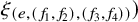
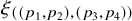 $\xi _{((p_1,p_2),(p_3,p_4))}$
at
$\xi _{((p_1,p_2),(p_3,p_4))}$
at
 $[{ \mathtt C}]$
is the signed length of the intersection of these two paths. Let
$[{ \mathtt C}]$
is the signed length of the intersection of these two paths. Let
 $\Gamma $
be a combinatorial type of cycle-rigidified n-marked genus-g curves, let
$\Gamma $
be a combinatorial type of cycle-rigidified n-marked genus-g curves, let
 $\widetilde \Gamma $
denote the universal covering space of
$\widetilde \Gamma $
denote the universal covering space of
 $\Gamma $
, and let
$\Gamma $
, and let
 $T\subset \widetilde \Gamma $
be a connected open subset all of whose vertices have genus
$T\subset \widetilde \Gamma $
be a connected open subset all of whose vertices have genus
 $0$
. Note that T is automatically a tree, that is
$0$
. Note that T is automatically a tree, that is
 $h^1(T)=0$
, and its leaves are open edge segments. For every combinatorial type
$h^1(T)=0$
, and its leaves are open edge segments. For every combinatorial type
 $\Gamma '$
specializing to
$\Gamma '$
specializing to
 $\Gamma $
, the preimage
$\Gamma $
, the preimage
 $T'$
of T under the induced retraction
$T'$
of T under the induced retraction
 $\widetilde \Gamma '\to \widetilde \Gamma $
of universal covers is a connected open subset of
$\widetilde \Gamma '\to \widetilde \Gamma $
of universal covers is a connected open subset of
 $\widetilde \Gamma '$
not containing higher-genus vertices, and the retraction induces a bijection between the leaves of
$\widetilde \Gamma '$
not containing higher-genus vertices, and the retraction induces a bijection between the leaves of
 $T'$
and the leaves of T. Forgetting the rest of the curve, this produces for every
$T'$
and the leaves of T. Forgetting the rest of the curve, this produces for every
 $\Gamma '$
specializing to
$\Gamma '$
specializing to
 $\Gamma $
a map
$\Gamma $
a map
 $\sigma _{\Gamma '}^\diamond \to \overline {\mathcal M}^{\mathrm {trop}}_{0, m}$
, where m is the number of leaves of T. Given a quadruple
$\sigma _{\Gamma '}^\diamond \to \overline {\mathcal M}^{\mathrm {trop}}_{0, m}$
, where m is the number of leaves of T. Given a quadruple
 $((p_1,p_2),(p_3,p_4))$
of distinct leaves of T, we can postcompose with the forgetful morphism
$((p_1,p_2),(p_3,p_4))$
of distinct leaves of T, we can postcompose with the forgetful morphism
 $\overline {\mathcal M}^{\mathrm {trop}}_{0,m}\to \overline {\mathcal M}^{\mathrm {trop}}_{0,4}$
that forgets all but the marks
$\overline {\mathcal M}^{\mathrm {trop}}_{0,m}\to \overline {\mathcal M}^{\mathrm {trop}}_{0,4}$
that forgets all but the marks
 $p_1,\ldots ,p_4$
. From
$p_1,\ldots ,p_4$
. From
 $\overline {\mathcal M}^{\mathrm {trop}}_{0,4}$
we can then pull-back the cross ratio function
$\overline {\mathcal M}^{\mathrm {trop}}_{0,4}$
we can then pull-back the cross ratio function
 $\xi _{((p_1,p_2),(p_3,p_4))}$
to obtain a function on
$\xi _{((p_1,p_2),(p_3,p_4))}$
to obtain a function on
 $\sigma _{\Gamma '}$
. For different
$\sigma _{\Gamma '}$
. For different
 $\Gamma '\to \Gamma $
, these functions glue together and define a cross ratio function
$\Gamma '\to \Gamma $
, these functions glue together and define a cross ratio function
 $\xi _{(T,(p_1,p_2),(p_3,p_4))}$
on a neighborhood of
$\xi _{(T,(p_1,p_2),(p_3,p_4))}$
on a neighborhood of
 $\sigma _\Gamma ^\diamond $
. This is the cross ratio function
$\sigma _\Gamma ^\diamond $
. This is the cross ratio function
 $\xi _c$
associated to the cross ratio datum
$\xi _c$
associated to the cross ratio datum
 $c=(T,(p_1,p_2),(p_3,p_4))$
(the tuple c is not literally a cross ratio datum in the sense of [Reference Cavalieri, Gross and Markwig6, Definition 4.8], but there is a natural induced cross ratio datum). The affine structure of
$c=(T,(p_1,p_2),(p_3,p_4))$
(the tuple c is not literally a cross ratio datum in the sense of [Reference Cavalieri, Gross and Markwig6, Definition 4.8], but there is a natural induced cross ratio datum). The affine structure of
 ${\overline {\mathcal V}_{g,n}}$
is the sheaf generated by cross ratio functions and constants. It is in fact generated by constants and the cross ratio functions associated to primitive cross ratio data: these correspond to the cases where T is a neighborhood of a single vertex v or of a single edge e. The four markings
${\overline {\mathcal V}_{g,n}}$
is the sheaf generated by cross ratio functions and constants. It is in fact generated by constants and the cross ratio functions associated to primitive cross ratio data: these correspond to the cases where T is a neighborhood of a single vertex v or of a single edge e. The four markings
 $p_1,\ldots ,p_4$
are induced by two pairs of flags
$p_1,\ldots ,p_4$
are induced by two pairs of flags
 $((f_1,f_2),(f_3,f_4))$
at v (resp. at the end points of e) and we write
$((f_1,f_2),(f_3,f_4))$
at v (resp. at the end points of e) and we write
 $c_{((f_1,f_2),(f_3,f_4))}$
(resp.
$c_{((f_1,f_2),(f_3,f_4))}$
(resp.
 $c_{(e,(f_1,f_2),(f_3,f_4))}$
) for the cross ratio datum induced by
$c_{(e,(f_1,f_2),(f_3,f_4))}$
) for the cross ratio datum induced by
 $(T,(p_1,p_2),(p_3,p_4))$
in the two respective cases and
$(T,(p_1,p_2),(p_3,p_4))$
in the two respective cases and
 $\xi _{((f_1,f_2),(f_3,f_4))}$
(resp.
$\xi _{((f_1,f_2),(f_3,f_4))}$
(resp.
 $\xi _{(e,(f_1,f_2),(f_3,f_4))})$
for the associated cross ratio functions.
$\xi _{(e,(f_1,f_2),(f_3,f_4))})$
for the associated cross ratio functions.
With these affine structures, the forgetful map
 $\mu _\star \colon {\overline {\mathcal V}_{g,n\sqcup \{\star \}}}\to {\overline {\mathcal V}_{g,n}}$
is a morphism of tropical spaces, but not a family of tropical curves. What fails is the condition on the fibers: it is true that all functions on
$\mu _\star \colon {\overline {\mathcal V}_{g,n\sqcup \{\star \}}}\to {\overline {\mathcal V}_{g,n}}$
is a morphism of tropical spaces, but not a family of tropical curves. What fails is the condition on the fibers: it is true that all functions on
 ${\overline {\mathcal V}_{g,n\sqcup \{\star \}}}$
are harmonic on the fibers, but not every harmonic function on a fiber is the restriction of an affine function.
${\overline {\mathcal V}_{g,n\sqcup \{\star \}}}$
are harmonic on the fibers, but not every harmonic function on a fiber is the restriction of an affine function.
2.2 Cone complexes and toroidal embeddings
We recall how to associate a cone complex to a toroidal embedding without self intersections. The original reference is [Reference Kempf, Faye Knudsen, Mumford and Saint-Donat18], where what we call cone complex was called conical polyhedral complex with integral structures, and we refer there and to [Reference Abramovich, Caporaso and Payne1, Reference Ulirsch25, Reference Kajiwara16, Reference Cavalieri, Chan, Ulirsch and Wise5] for a more detailed treatment.
A (abstract) cone is a pair
 $(\sigma , M^\sigma )$
consisting of a topological space
$(\sigma , M^\sigma )$
consisting of a topological space
 $\sigma $
and a lattice
$\sigma $
and a lattice
 $M^\sigma $
of real-valued continuous functions on
$M^\sigma $
of real-valued continuous functions on
 $\sigma $
with the property that the natural map
$\sigma $
with the property that the natural map ![]() maps
maps
 $\sigma $
homeomorphically onto its image, a strictly convex rational polyhedral cone in
$\sigma $
homeomorphically onto its image, a strictly convex rational polyhedral cone in ![]() . If we denote
. If we denote
 $M^\sigma _+=\{m\in M^\sigma : m\geq 0\}$
, then the image of
$M^\sigma _+=\{m\in M^\sigma : m\geq 0\}$
, then the image of
 $\sigma $
in
$\sigma $
in ![]() is precisely
is precisely ![]() . The faces of
. The faces of
 $(\sigma ,M^\sigma )$
are the pairs
$(\sigma ,M^\sigma )$
are the pairs
 $(\tau , \{m\vert _\tau :m\in M^\sigma \})$
, where
$(\tau , \{m\vert _\tau :m\in M^\sigma \})$
, where
 $\tau $
is a face of
$\tau $
is a face of
 $\sigma $
. The relative interior of a cone
$\sigma $
. The relative interior of a cone
 $\sigma $
is the complement of all its proper faces; we denote it by
$\sigma $
is the complement of all its proper faces; we denote it by
 $\sigma ^\diamond $
. A cone complex is pair
$\sigma ^\diamond $
. A cone complex is pair
 $(\vert \Sigma \vert ,\Sigma )$
consisting of a topological space
$(\vert \Sigma \vert ,\Sigma )$
consisting of a topological space
 $\vert \Sigma \vert $
and a collection
$\vert \Sigma \vert $
and a collection
 $\Sigma $
of cones whose underlying sets are closed subsets of
$\Sigma $
of cones whose underlying sets are closed subsets of
 $\vert \Sigma \vert $
and such that
$\vert \Sigma \vert $
and such that
 $\vert \Sigma \vert =\bigsqcup _{\sigma \in \Sigma }\sigma ^\diamond $
. Moreover, the set
$\vert \Sigma \vert =\bigsqcup _{\sigma \in \Sigma }\sigma ^\diamond $
. Moreover, the set
 $\Sigma $
is closed under taking faces and intersections. A continuous function
$\Sigma $
is closed under taking faces and intersections. A continuous function
 $\phi $
on a subset
$\phi $
on a subset
 $U\subseteq \Sigma $
is strict piecewise linear if for all
$U\subseteq \Sigma $
is strict piecewise linear if for all
 $\sigma \in \Sigma $
there exists
$\sigma \in \Sigma $
there exists
 $m\in M^\sigma $
and
$m\in M^\sigma $
and ![]() with
with
 $\phi \vert _{\sigma \cap U}=m\vert _{\sigma \cap U}+c$
. We denote the group of strict piecewise linear functions on U by
$\phi \vert _{\sigma \cap U}=m\vert _{\sigma \cap U}+c$
. We denote the group of strict piecewise linear functions on U by
 ${\mathrm {sPL}}_\Sigma (U)$
.
${\mathrm {sPL}}_\Sigma (U)$
.
For a cone
 $\sigma $
, the extended cone
$\sigma $
, the extended cone
 $\overline \sigma $
is given by
$\overline \sigma $
is given by ![]() . The extended cones of the cones in a cone complex
. The extended cones of the cones in a cone complex
 $\Sigma $
can be glued to an extended cone complex
$\Sigma $
can be glued to an extended cone complex
 $\overline \Sigma $
. The extended cone complex
$\overline \Sigma $
. The extended cone complex
 $\Sigma $
has a natural stratification
$\Sigma $
has a natural stratification
 $\overline \Sigma =\bigsqcup _{\tau \prec \sigma \in \Sigma }\sigma /\tau $
. Any choice of generators of
$\overline \Sigma =\bigsqcup _{\tau \prec \sigma \in \Sigma }\sigma /\tau $
. Any choice of generators of
 $M^\sigma _+$
induces an embedding of an extended cone
$M^\sigma _+$
induces an embedding of an extended cone
 $\overline \sigma $
into
$\overline \sigma $
into ![]() for some
for some ![]() and thus
and thus
 $\overline \sigma $
obtains the structure of a TPL-space. Declaring a function on an extended cone complex to be piecewise linear if and only if its restrictions to all extended cones of the complex are piecewise linear defines a TPL-structure on any extended cone complex.
$\overline \sigma $
obtains the structure of a TPL-space. Declaring a function on an extended cone complex to be piecewise linear if and only if its restrictions to all extended cones of the complex are piecewise linear defines a TPL-structure on any extended cone complex.
A toroidal embedding without self-intersection is a pair
 $(X_0,X)$
consisting of a variety X and an open subset
$(X_0,X)$
consisting of a variety X and an open subset
 $X_0\subseteq X$
that locally looks like the inclusion of the big torus into a toric variety. More precisely, for every point
$X_0\subseteq X$
that locally looks like the inclusion of the big torus into a toric variety. More precisely, for every point
 $x\in X$
there exists a toric chart, that is, an open neighborhood U of x, a toric variety Y with big open torus T, and an étale morphism
$x\in X$
there exists a toric chart, that is, an open neighborhood U of x, a toric variety Y with big open torus T, and an étale morphism
 $f\colon U\to Y$
with
$f\colon U\to Y$
with
 $f^{-1}T=U\cap X_0$
.Footnote 3 The toroidal embedding X has an associated cone complex
$f^{-1}T=U\cap X_0$
.Footnote 3 The toroidal embedding X has an associated cone complex
 $\Sigma _X$
, with each
$\Sigma _X$
, with each
 $\sigma \in \Sigma _X$
corresponding to a stratum
$\sigma \in \Sigma _X$
corresponding to a stratum
 $O(\sigma )$
in the stratification of X induced by the toric charts. If we denote by
$O(\sigma )$
in the stratification of X induced by the toric charts. If we denote by
 $V(\sigma )$
the closure of
$V(\sigma )$
the closure of
 $O(\sigma )$
, the strata closures
$O(\sigma )$
, the strata closures
 $V(\rho )$
for rays
$V(\rho )$
for rays
 $\rho \in \Sigma _X(1)$
are the irreducible components of the boundary
$\rho \in \Sigma _X(1)$
are the irreducible components of the boundary
 $X\setminus X_0$
, and all other strata are connected components of
$X\setminus X_0$
, and all other strata are connected components of
 $\bigcap _{\rho \in I}V(\rho )\setminus \bigcup _{\rho \notin I}V(\rho )$
for subsets
$\bigcap _{\rho \in I}V(\rho )\setminus \bigcup _{\rho \notin I}V(\rho )$
for subsets
 $I\subseteq \Sigma _X(1)$
. For a cone
$I\subseteq \Sigma _X(1)$
. For a cone
 $\sigma \in \Sigma _X$
, the monoid
$\sigma \in \Sigma _X$
, the monoid
 $M^\sigma $
is naturally identified with the set of effective boundary Cartier divisors near
$M^\sigma $
is naturally identified with the set of effective boundary Cartier divisors near
 $O(\sigma )$
. In particular, the functions in
$O(\sigma )$
. In particular, the functions in
 ${\mathrm {sPL}}(\Sigma )$
with trivial constant part are in natural bijection with boundary Cartier divisors on X.
${\mathrm {sPL}}(\Sigma )$
with trivial constant part are in natural bijection with boundary Cartier divisors on X.
A dominant toroidal morphism of toroidal embeddings X and Y is a dominant morphism
 $X\to Y$
of schemes that can be expressed as a morphism of toric varieties in toric charts. A toroidal morphism from X to Y is any morphism of schemes
$X\to Y$
of schemes that can be expressed as a morphism of toric varieties in toric charts. A toroidal morphism from X to Y is any morphism of schemes
 $X\to Y$
that factors through a dominant toroidal morphism
$X\to Y$
that factors through a dominant toroidal morphism
 $X\to V(\sigma )$
for some
$X\to V(\sigma )$
for some
 $\sigma \in \Sigma _Y$
.Footnote 4 A dominant toroidal morphism
$\sigma \in \Sigma _Y$
.Footnote 4 A dominant toroidal morphism
 $f\colon X\to Y$
induces a morphism
$f\colon X\to Y$
induces a morphism
 ${\mathtt {Trop}}(f)\colon \Sigma _X\to \Sigma _Y$
, that is a continuous map
${\mathtt {Trop}}(f)\colon \Sigma _X\to \Sigma _Y$
, that is a continuous map
 $\vert \Sigma _X\vert \to \vert \Sigma _Y\vert $
mapping the cones of
$\vert \Sigma _X\vert \to \vert \Sigma _Y\vert $
mapping the cones of
 $\Sigma _X$
linearly into cones of
$\Sigma _X$
linearly into cones of
 $\Sigma _Y$
. The map
$\Sigma _Y$
. The map
 ${\mathtt {Trop}}(f)$
extends to a morphism on the extended cone complexes. For
${\mathtt {Trop}}(f)$
extends to a morphism on the extended cone complexes. For
 $\tau \in \Sigma _Y$
, we have a natural identification of
$\tau \in \Sigma _Y$
, we have a natural identification of
 $\Sigma _{V(\tau )}$
with the subcomplex
$\Sigma _{V(\tau )}$
with the subcomplex
 $\bigcup _{\tau \subseteq \sigma \in \Sigma _Y} \sigma /\tau $
of
$\bigcup _{\tau \subseteq \sigma \in \Sigma _Y} \sigma /\tau $
of
 $\overline \Sigma _Y$
. In particular, for a not necessarily dominant toroidal morphism
$\overline \Sigma _Y$
. In particular, for a not necessarily dominant toroidal morphism
 $f\colon X\to Y$
there is an induced morphism
$f\colon X\to Y$
there is an induced morphism
 ${\mathtt {Trop}}(f)\colon \overline \Sigma _X\to \overline \Sigma _Y$
.
${\mathtt {Trop}}(f)\colon \overline \Sigma _X\to \overline \Sigma _Y$
.
2.3 Tropical cycles
We present the notion of tropical cycles and their intersection pairing with tropical divisors in the generality developed in [Reference Cavalieri, Gross and Markwig6].
A k-weight on a cone complex
 $\Sigma $
is an equivalence class of pairs
$\Sigma $
is an equivalence class of pairs
 $(\Delta ,c)$
, where
$(\Delta ,c)$
, where
 $\Delta $
is a proper subdivision of
$\Delta $
is a proper subdivision of
 $\Sigma $
and
$\Sigma $
and ![]() is a map. Here,
is a map. Here,
 $\Delta (k)$
denote the set of k-dimensional cones of
$\Delta (k)$
denote the set of k-dimensional cones of
 $\Delta $
, and the equivalence relation is induced by compatibility under refinements of
$\Delta $
, and the equivalence relation is induced by compatibility under refinements of
 $\Delta $
. Given an affine structure
$\Delta $
. Given an affine structure
 $\operatorname {\mathrm {Aff}}_\Sigma $
, which we assume to satisfy the condition that
$\operatorname {\mathrm {Aff}}_\Sigma $
, which we assume to satisfy the condition that
 $\Omega ^1_\Sigma $
is constant on all cones, we define the balancing condition for weights as follows: a
$\Omega ^1_\Sigma $
is constant on all cones, we define the balancing condition for weights as follows: a
 $1$
-weight represented by
$1$
-weight represented by
 $(\Delta , c)$
is balanced with respect to an affine function
$(\Delta , c)$
is balanced with respect to an affine function
 $\phi \in \operatorname {\mathrm {Aff}}_\Sigma (\Sigma )$
with
$\phi \in \operatorname {\mathrm {Aff}}_\Sigma (\Sigma )$
with
 $\phi (0_\Sigma )=0$
(here,
$\phi (0_\Sigma )=0$
(here,
 $0_\Sigma $
refers to the cone point of
$0_\Sigma $
refers to the cone point of
 $\Sigma $
), if we have
$\Sigma $
), if we have
 $\sum _{\rho \in \Delta (1)} \phi (u_\rho )\cdot c(\rho )=0$
, where
$\sum _{\rho \in \Delta (1)} \phi (u_\rho )\cdot c(\rho )=0$
, where
 $u_\rho $
denotes the primitive lattice generator of a ray
$u_\rho $
denotes the primitive lattice generator of a ray
 $\rho $
. We say that c is balanced if it is balanced with respect to every
$\rho $
. We say that c is balanced if it is balanced with respect to every
 $\phi \in \operatorname {\mathrm {Aff}}_\Sigma (\Sigma )$
with
$\phi \in \operatorname {\mathrm {Aff}}_\Sigma (\Sigma )$
with
 $\phi (0_\Sigma )=0$
. More generally, a k-weight represented by
$\phi (0_\Sigma )=0$
. More generally, a k-weight represented by
 $(\Delta , c)$
is balanced if for every
$(\Delta , c)$
is balanced if for every
 $(k-1)$
-dimensional cone
$(k-1)$
-dimensional cone
 $\tau \in \Delta $
and every affine function
$\tau \in \Delta $
and every affine function
 $\phi \in \operatorname {\mathrm {Aff}}_\Sigma (\Delta ^\tau )$
with
$\phi \in \operatorname {\mathrm {Aff}}_\Sigma (\Delta ^\tau )$
with
 $\phi \vert _\tau =0$
, the induced
$\phi \vert _\tau =0$
, the induced
 $1$
-weight
$1$
-weight
 $\overline c$
on
$\overline c$
on
 $\Sigma ^\tau /\tau $
is balanced with respect to the induced function
$\Sigma ^\tau /\tau $
is balanced with respect to the induced function
 $\overline \phi $
. Note that the balancing condition is independent of the choice of representative
$\overline \phi $
. Note that the balancing condition is independent of the choice of representative
 $(\Delta ,c)$
. A balanced k-weight is called a tropical k-cycle.
$(\Delta ,c)$
. A balanced k-weight is called a tropical k-cycle.
We say a function
 $\phi \in {\mathrm {sPL}}_\Sigma (\Sigma )$
is combinatorially principal at the cone
$\phi \in {\mathrm {sPL}}_\Sigma (\Sigma )$
is combinatorially principal at the cone
 $\sigma $
, and write
$\sigma $
, and write
 $\phi \in {\mathrm {CP}}(\sigma )$
if there exists
$\phi \in {\mathrm {CP}}(\sigma )$
if there exists
 $\chi \in \operatorname {\mathrm {Aff}}_\Sigma (\Sigma ^\sigma )$
with
$\chi \in \operatorname {\mathrm {Aff}}_\Sigma (\Sigma ^\sigma )$
with
 $\chi \vert _\sigma =\phi \vert _\sigma $
. We say
$\chi \vert _\sigma =\phi \vert _\sigma $
. We say
 $\phi $
is combinatorially principal if it is combinatorially principal at every cone
$\phi $
is combinatorially principal if it is combinatorially principal at every cone
 $\sigma \in \Sigma $
, and denote the group of combinatorially principal functions on
$\sigma \in \Sigma $
, and denote the group of combinatorially principal functions on
 $\Sigma $
by
$\Sigma $
by
 ${\mathrm {CP}}(\Sigma )$
. For a function
${\mathrm {CP}}(\Sigma )$
. For a function
 $\phi \in {\mathrm {sPL}}_\Sigma (\Sigma )$
and a tropical
$\phi \in {\mathrm {sPL}}_\Sigma (\Sigma )$
and a tropical
 $1$
-cycle A represented by
$1$
-cycle A represented by
 $(\Delta ,c)$
, the intersection product
$(\Delta ,c)$
, the intersection product
 $\phi \cdot A$
is the unique
$\phi \cdot A$
is the unique
 $0$
-cycle whose weight at the origin is given by
$0$
-cycle whose weight at the origin is given by
 $$ \begin{align} -\sum_{\rho\in \Delta(1)} \mathrm{slope}_\rho(\phi)c(\rho) , \end{align} $$
where
 $-\mathrm {slope}_\rho (\phi )=-\phi (u_\rho )$
is the incoming slope of
$-\mathrm {slope}_\rho (\phi )=-\phi (u_\rho )$
is the incoming slope of
 $\phi $
at the origin, as required by the
$\phi $
at the origin, as required by the
 $\min $
convention. This only depends on the class of
$\min $
convention. This only depends on the class of
 $\phi \in {\mathrm {sPL}}_\Sigma (\Sigma )/\operatorname {\mathrm {Aff}}_\Sigma (\Sigma )$
. Let
$\phi \in {\mathrm {sPL}}_\Sigma (\Sigma )/\operatorname {\mathrm {Aff}}_\Sigma (\Sigma )$
. Let
 $\phi \in {\mathrm {CP}}(\Sigma )$
and let
$\phi \in {\mathrm {CP}}(\Sigma )$
and let
 $A=[(\Delta ,c)]$
be a tropical k-cycle on
$A=[(\Delta ,c)]$
be a tropical k-cycle on
 $\Sigma $
. The intersection product
$\Sigma $
. The intersection product
 $\phi \cdot A$
is the tropical cycle represented by the
$\phi \cdot A$
is the tropical cycle represented by the
 $(k-1)$
-weight whose weight on
$(k-1)$
-weight whose weight on
 $\tau \in \Delta (k-1)$
is given by the weight at the origin of
$\tau \in \Delta (k-1)$
is given by the weight at the origin of
 $\overline \phi \cdot \overline c$
, where
$\overline \phi \cdot \overline c$
, where
 $\overline c$
is the tropical
$\overline c$
is the tropical
 $1$
-cycle on
$1$
-cycle on
 $\Delta ^\tau /\tau $
induced by c and
$\Delta ^\tau /\tau $
induced by c and
 $\overline \phi $
is the function on
$\overline \phi $
is the function on
 $\Delta ^\tau /\tau $
induced by
$\Delta ^\tau /\tau $
induced by
 $\phi -\chi $
for some
$\phi -\chi $
for some
 $\chi \in \operatorname {\mathrm {Aff}}_\Sigma (\Sigma )$
with
$\chi \in \operatorname {\mathrm {Aff}}_\Sigma (\Sigma )$
with
 $\chi \vert _\tau =\phi \vert _\tau $
. By construction,
$\chi \vert _\tau =\phi \vert _\tau $
. By construction,
 $\phi \cdot A$
depends only on the class of
$\phi \cdot A$
depends only on the class of
 $\phi $
in
$\phi $
in
 ${\mathrm {CP}}(\Sigma )/\operatorname {\mathrm {Aff}}_\Sigma (\Sigma )$
.
${\mathrm {CP}}(\Sigma )/\operatorname {\mathrm {Aff}}_\Sigma (\Sigma )$
.
We just presented the local theory of tropical cycles, which is all we need in this paper. These concepts can be globalized: there exists a sheaf
 $Z_k$
of tropical k-cycles on tropical spaces, a sheaf
$Z_k$
of tropical k-cycles on tropical spaces, a sheaf
 ${\mathrm {CP}}$
(denoted by
${\mathrm {CP}}$
(denoted by
 $\mathrm {Rat}$
in [Reference Cavalieri, Gross and Markwig6, Definition 6.3]) of combinatorially principal functions, and an intersection-pairing
$\mathrm {Rat}$
in [Reference Cavalieri, Gross and Markwig6, Definition 6.3]) of combinatorially principal functions, and an intersection-pairing
that locally looks like the pairing in the case of cone complexes with affine structure. The sheaf
 ${\mathrm {CP}}/\operatorname {\mathrm {Aff}}$
is the sheaf of combinatorially principal tropical Cartier divisors, sitting inside the sheaf
${\mathrm {CP}}/\operatorname {\mathrm {Aff}}$
is the sheaf of combinatorially principal tropical Cartier divisors, sitting inside the sheaf
 ${\mathrm {PL}}^{\mathrm {fin}}/\operatorname {\mathrm {Aff}}$
of tropical Cartier divisors. The k-th tropical Chow group
${\mathrm {PL}}^{\mathrm {fin}}/\operatorname {\mathrm {Aff}}$
of tropical Cartier divisors. The k-th tropical Chow group
 $A_k({ \mathtt X})$
of a tropical space
$A_k({ \mathtt X})$
of a tropical space
 ${ \mathtt X}$
is given by
${ \mathtt X}$
is given by
2.4 Tropical line bundles and psi classes
A tropical line bundle on a tropical space
 ${ \mathtt X}$
is an
${ \mathtt X}$
is an
 $\operatorname {\mathrm {Aff}}_{ \mathtt X}$
-torsor. Equivalently, it is a morphism
$\operatorname {\mathrm {Aff}}_{ \mathtt X}$
-torsor. Equivalently, it is a morphism
 ${ \mathtt L}\to { \mathtt X}$
whose fibers are
${ \mathtt L}\to { \mathtt X}$
whose fibers are ![]() -torsors and which locally trivializes: it is locally isomorphic to
-torsors and which locally trivializes: it is locally isomorphic to ![]() as tropical spaces, and the isomorphism is an isomorphism of
as tropical spaces, and the isomorphism is an isomorphism of ![]() -torsors on each fiber. One can translate the two notions into each other by associating to a line bundle
-torsors on each fiber. One can translate the two notions into each other by associating to a line bundle
 ${ \mathtt L}\to { \mathtt X}$
the sheaf
${ \mathtt L}\to { \mathtt X}$
the sheaf ![]() of isomorphisms with the trivial line bundle, which is an
of isomorphisms with the trivial line bundle, which is an
 $\operatorname {\mathrm {Aff}}_{ \mathtt X}$
-torsor because
$\operatorname {\mathrm {Aff}}_{ \mathtt X}$
-torsor because ![]() .
.
By [Reference Jell, Rau and Shaw15, Lemma 4.5], every tropical line bundle
 ${ \mathtt L}$
has a piecewise linear section. Any such section defines a tropical Cartier divisor
${ \mathtt L}$
has a piecewise linear section. Any such section defines a tropical Cartier divisor
 $\mathtt D$
whose associated tropical line bundle is isomorphic to
$\mathtt D$
whose associated tropical line bundle is isomorphic to
 ${ \mathtt L}$
. In the language of torsors, the existence of a piecewise linear section means that given any
${ \mathtt L}$
. In the language of torsors, the existence of a piecewise linear section means that given any
 $\operatorname {\mathrm {Aff}}_{ \mathtt X}$
-torsor, the associated
$\operatorname {\mathrm {Aff}}_{ \mathtt X}$
-torsor, the associated
 ${\mathrm {PL}}$
-torsor is trivial. However, the associated
${\mathrm {PL}}$
-torsor is trivial. However, the associated
 ${\mathrm {CP}}$
-torsor is not necessarily trivial, that is the line bundle does not necessarily have a combinatorially principal section (i.e., the tropical Cartier divisor
${\mathrm {CP}}$
-torsor is not necessarily trivial, that is the line bundle does not necessarily have a combinatorially principal section (i.e., the tropical Cartier divisor
 $\mathtt D$
from above is not necessarily combinatorially principal). If a tropical line bundle
$\mathtt D$
from above is not necessarily combinatorially principal). If a tropical line bundle
 ${ \mathtt L}$
on a tropical space
${ \mathtt L}$
on a tropical space
 ${ \mathtt X}$
has a combinatorially principal section, any choice of such section defines the same element in
${ \mathtt X}$
has a combinatorially principal section, any choice of such section defines the same element in
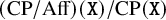 $({\mathrm {CP}}/\operatorname {\mathrm {Aff}})({ \mathtt X})/{\mathrm {CP}}({ \mathtt X})$
(a combinatorially principal tropical Cartier divisor modulo linear equivalence), and this element defines a map
$({\mathrm {CP}}/\operatorname {\mathrm {Aff}})({ \mathtt X})/{\mathrm {CP}}({ \mathtt X})$
(a combinatorially principal tropical Cartier divisor modulo linear equivalence), and this element defines a map
 $$ \begin{align} c_1({ \mathtt L})\colon A_*({ \mathtt X})\to A_{*-1}({ \mathtt X}) \end{align} $$
via the intersection pairing. The map
 $c_1({ \mathtt L})$
is called the first Chern class of
$c_1({ \mathtt L})$
is called the first Chern class of
 ${ \mathtt L}$
. Given
${ \mathtt L}$
. Given
 $\alpha \in A_\ast ({ \mathtt X})$
, we denote
$\alpha \in A_\ast ({ \mathtt X})$
, we denote
 $c_1({ \mathtt L})(\alpha )$
by
$c_1({ \mathtt L})(\alpha )$
by
 $c_1({ \mathtt L}) \frown \alpha $
to avoid proliferation of nested parentheses.
$c_1({ \mathtt L}) \frown \alpha $
to avoid proliferation of nested parentheses.
We recall the construction of tropical
 $\psi $
classes from [Reference Cavalieri, Gross and Markwig6]. Given a family of n-marked, stable tropical curves
$\psi $
classes from [Reference Cavalieri, Gross and Markwig6]. Given a family of n-marked, stable tropical curves
 $\overline { \mathtt C}\to \overline { \mathtt B}$
, for every
$\overline { \mathtt C}\to \overline { \mathtt B}$
, for every
 $1\leq i\leq n$
and
$1\leq i\leq n$
and ![]() the i-th section
the i-th section
 ${\mathtt s}_i\colon \overline { \mathtt B}\to \overline { \mathtt C}$
defines a tropical line bundle
${\mathtt s}_i\colon \overline { \mathtt B}\to \overline { \mathtt C}$
defines a tropical line bundle
 $\operatorname {\mathrm {Aff}}_{\overline { \mathtt C}}(k {\mathtt s}_i)$
in the form of an
$\operatorname {\mathrm {Aff}}_{\overline { \mathtt C}}(k {\mathtt s}_i)$
in the form of an
 $\operatorname {\mathrm {Aff}}_{\overline { \mathtt C}}$
-torsor on the total space
$\operatorname {\mathrm {Aff}}_{\overline { \mathtt C}}$
-torsor on the total space
 $\overline { \mathtt C}$
. Namely, every point in the image of
$\overline { \mathtt C}$
. Namely, every point in the image of
 ${\mathtt s}_i$
is the infinite point of a leg in its fiber. Therefore, we can define
${\mathtt s}_i$
is the infinite point of a leg in its fiber. Therefore, we can define
 $\operatorname {\mathrm {Aff}}_{\overline { \mathtt C}}(k{\mathtt s}_i)$
as the subsheaf of
$\operatorname {\mathrm {Aff}}_{\overline { \mathtt C}}(k{\mathtt s}_i)$
as the subsheaf of
 $\iota _*\operatorname {\mathrm {Aff}}_{\overline { \mathtt C}\setminus {\mathtt s}_i(\overline { \mathtt B})}$
, where
$\iota _*\operatorname {\mathrm {Aff}}_{\overline { \mathtt C}\setminus {\mathtt s}_i(\overline { \mathtt B})}$
, where
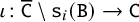 $\iota \colon \overline { \mathtt C}\setminus {\mathtt s}_i({ \mathtt B})\to \mathtt C$
is the inclusion, of all functions whose slope on the leg approaching
$\iota \colon \overline { \mathtt C}\setminus {\mathtt s}_i({ \mathtt B})\to \mathtt C$
is the inclusion, of all functions whose slope on the leg approaching
 ${\mathtt s}_i$
is
${\mathtt s}_i$
is
 $-k$
. The i-th tropical cotangent line bundle
$-k$
. The i-th tropical cotangent line bundle ![]() is the line bundle on
is the line bundle on
 $\overline { \mathtt B}$
defined as
$\overline { \mathtt B}$
defined as
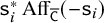 ${\mathtt s}_i^*\operatorname {\mathrm {Aff}}_{\overline { \mathtt C}}(-{\mathtt s}_i)$
.
${\mathtt s}_i^*\operatorname {\mathrm {Aff}}_{\overline { \mathtt C}}(-{\mathtt s}_i)$
.
If ![]() is the i-the cotangent bundle of a marked family of tropical curves, we call the first Chern class of
is the i-the cotangent bundle of a marked family of tropical curves, we call the first Chern class of
 ${ \mathtt L}$
the i-th
${ \mathtt L}$
the i-th
 $\psi $
class and denote it by
$\psi $
class and denote it by
3 Affine Structures for Tropicalizations
This section contains the core technical definitions and constructions. Given a toroidal variety X, we endow its cone complex with an affine structure, calling the result the tropicalization of X. Tropicalization becomes a functor valued in the category of tropical spaces. To simplify the exposition, we initially make the following seemingly strong assumption:
 $(\ast )$
there are no self-intersections among the toroidal strata or multiple intersections among pairs of strata.
$(\ast )$
there are no self-intersections among the toroidal strata or multiple intersections among pairs of strata.
We prove that the affine structure induced by tropicalization is invariant under log modifications and explain in Remark 3.9 how this allows us to remove such hypothesis without loss of generality.
3.1 Affine structures on cone complexes
Let
 $\Sigma $
be a cone complex. A subcomplex S of
$\Sigma $
be a cone complex. A subcomplex S of
 $\Sigma $
is a union
$\Sigma $
is a union
 $$ \begin{align}S = \bigcup_{\sigma\in I}\sigma^\diamond,\end{align} $$
where I is a subset of cones of
 $\Sigma $
. We say that S is an open (resp. closed) subcomplex of
$\Sigma $
. We say that S is an open (resp. closed) subcomplex of
 $\Sigma $
if it defines an open (resp. closed) set.
$\Sigma $
if it defines an open (resp. closed) set.
For a cone
 $\sigma \in \Sigma $
, we define the open star
$\sigma \in \Sigma $
, we define the open star
 $\Sigma ^\sigma $
of
$\Sigma ^\sigma $
of
 $\sigma $
to be the open subcomplex
$\sigma $
to be the open subcomplex
 $$ \begin{align} \Sigma^\sigma= \bigcup_{\sigma\subseteq \tau} \tau^\diamond , \end{align} $$
given by the union of the relative interiors of all cones containing
 $\sigma $
. The usual star of
$\sigma $
. The usual star of
 $\sigma $
, consisting of the union of all cones containing
$\sigma $
, consisting of the union of all cones containing
 $\sigma $
, is the closure of the open star, and we denote it by
$\sigma $
, is the closure of the open star, and we denote it by
 $\overline {\Sigma ^\sigma }.$
Footnote 5
$\overline {\Sigma ^\sigma }.$
Footnote 5
Let X be a toroidal variety satisfying
 $(\ast )$
, and
$(\ast )$
, and
 $\Sigma _X$
its cone complex as described in Section 2.2. Every
$\Sigma _X$
its cone complex as described in Section 2.2. Every
 $\sigma \in \Sigma _X$
corresponds to a stratum
$\sigma \in \Sigma _X$
corresponds to a stratum
 $O(\sigma )$
.
$O(\sigma )$
.
For a cone
 $\sigma \in \Sigma _X$
we denote by
$\sigma \in \Sigma _X$
we denote by
 $X_\sigma $
the open neighborhood of
$X_\sigma $
the open neighborhood of
 $V(\sigma )$
given by
$V(\sigma )$
given by
 $$ \begin{align} X_\sigma=\bigcup_{\tau\in \overline{\Sigma_X^\sigma}} O(\tau) . \end{align} $$
A strict piecewise linear function
 $\phi $
on
$\phi $
on
 $\Sigma _X^\sigma $
determines a Cartier divisor, and consequently an invertible sheaf on
$\Sigma _X^\sigma $
determines a Cartier divisor, and consequently an invertible sheaf on
 $X_\sigma $
: extend
$X_\sigma $
: extend
 $\phi $
to
$\phi $
to
 $\overline {\Sigma _X^\sigma }$
by linearity, and for any ray
$\overline {\Sigma _X^\sigma }$
by linearity, and for any ray
 $\rho \in \overline {\Sigma _X^\sigma }$
denote the slope of
$\rho \in \overline {\Sigma _X^\sigma }$
denote the slope of
 $\phi |_{\rho }$
by
$\phi |_{\rho }$
by
 $\mathrm {slope}_{\rho }(\phi )$
. We define:
$\mathrm {slope}_{\rho }(\phi )$
. We define:
 $$ \begin{align} D_{X_\sigma}(\phi) = \sum_{\rho\in \overline{\Sigma_X^\sigma}} \mathrm{slope}_{\rho}(\phi) V(\rho) , & & \mathcal O_{X_{\sigma}}(\phi)= \mathcal O_{X_{\sigma}}\left(D_{X_\sigma}(\phi)\right). \end{align} $$
Definition 3.1. Let
 $\Sigma _X$
be the cone complex of a toroidal variety X, and
$\Sigma _X$
be the cone complex of a toroidal variety X, and
 $\sigma \in \Sigma _X$
.
$\sigma \in \Sigma _X$
.
An affine function at
 $\sigma $
is a strict piecewise linear function
$\sigma $
is a strict piecewise linear function
 $\phi $
on
$\phi $
on
 $\Sigma ^\sigma $
such that
$\Sigma ^\sigma $
such that
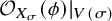 $\mathcal O_{X_{\sigma }}(\phi )\vert _{V(\sigma )}$
is trivial.
$\mathcal O_{X_{\sigma }}(\phi )\vert _{V(\sigma )}$
is trivial.
The affine structure
 $\operatorname {\mathrm {Aff}}_{\Sigma _X}$
on
$\operatorname {\mathrm {Aff}}_{\Sigma _X}$
on
 $\Sigma _X$
induced by X is defined to be the subsheaf of
$\Sigma _X$
induced by X is defined to be the subsheaf of
 ${\mathrm {PL}}^{\mathrm {fin}}_{\Sigma _X}$
generated by affine functions at cones
${\mathrm {PL}}^{\mathrm {fin}}_{\Sigma _X}$
generated by affine functions at cones
 $\sigma \in {\Sigma _X}$
.
$\sigma \in {\Sigma _X}$
.
As shown in the following lemma, affine functions in the sense of Definition 3.1 are closed under restriction, hence we are not generating any new sections of
 $\operatorname {\mathrm {Aff}}_\Sigma $
by restriction.
$\operatorname {\mathrm {Aff}}_\Sigma $
by restriction.
Lemma 3.2. Let
 $\sigma \in \Sigma $
, let
$\sigma \in \Sigma $
, let
 $\tau $
be a face of
$\tau $
be a face of
 $\sigma $
, and let
$\sigma $
, and let
 $\phi $
be an affine function at
$\phi $
be an affine function at
 $\tau $
. Then
$\tau $
. Then
 $\phi \vert _{\Sigma ^\sigma }$
is an affine function at
$\phi \vert _{\Sigma ^\sigma }$
is an affine function at
 $\sigma $
.
$\sigma $
.
Proof. Since
 $V(\sigma )$
is contained in
$V(\sigma )$
is contained in
 $V(\tau )$
,
$V(\tau )$
,
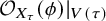 $\mathcal O_{X_\tau }(\phi )\vert _{V(\tau )}$
being trivial implies that the bundle
$\mathcal O_{X_\tau }(\phi )\vert _{V(\tau )}$
being trivial implies that the bundle
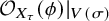 $\mathcal O_{X_\tau }(\phi )\vert _{V(\sigma )}$
is trivial as well. The assertion now follows from the fact that
$\mathcal O_{X_\tau }(\phi )\vert _{V(\sigma )}$
is trivial as well. The assertion now follows from the fact that
 $$ \begin{align} \mathcal{O}_{X_\tau}(\phi)\vert_{X_\sigma}=\mathcal{O}_{X_\sigma}(\phi\vert_{\Sigma_\sigma}) . \end{align} $$
Corollary 3.3. Let
 $\sigma \in \Sigma $
. Then
$\sigma \in \Sigma $
. Then
 $ \operatorname {\mathrm {Aff}}_\Sigma (\Sigma ^\sigma )$
consists precisely of affine functions at
$ \operatorname {\mathrm {Aff}}_\Sigma (\Sigma ^\sigma )$
consists precisely of affine functions at
 $\sigma $
.
$\sigma $
.
Proof. This is an immediate consequence of Lemma 3.2.
Remark 3.4. This notion of affine functions is related to the linear functions on Cartwright’s tropical complexes [Reference Cartwright4]. To compare the two notions, consider the situation where we are given a proper morphism ![]() such that X is smooth and connected and
such that X is smooth and connected and
 $\pi ^{-1}\{0\}$
is a reduced simple normal crossings divisor. In particular, the pair
$\pi ^{-1}\{0\}$
is a reduced simple normal crossings divisor. In particular, the pair ![]() defines a toroidal embedding and
defines a toroidal embedding and
 $\pi $
is a dominant toroidal morphism. We obtain an induced morphism
$\pi $
is a dominant toroidal morphism. We obtain an induced morphism ![]() of cone complexes and the linear functions of [Reference Cartwright4] are defined on the fiber
of cone complexes and the linear functions of [Reference Cartwright4] are defined on the fiber ![]() . To be linear in the sense of Cartwright, a function
. To be linear in the sense of Cartwright, a function
 $\chi $
on
$\chi $
on
 $\Delta $
has to satisfy the condition that for each
$\Delta $
has to satisfy the condition that for each
 $\sigma \in \Sigma $
with
$\sigma \in \Sigma $
with
 $V(\sigma )$
a curve, there exists a function
$V(\sigma )$
a curve, there exists a function
 $\phi \in {\mathrm {sPL}}(\Sigma ^\sigma )$
with
$\phi \in {\mathrm {sPL}}(\Sigma ^\sigma )$
with
 $$ \begin{align} \phi\vert_{\Delta\cap \Sigma^\sigma} &=\chi\vert_{\Delta\cap\Sigma^\sigma}, \qquad\text{and} \end{align} $$
 $$ \begin{align} \deg(\mathcal O_{X_\sigma}(\phi)\vert_{V(\sigma)}) &= 0. \end{align} $$
So Cartwright’s linearity is only checked locally around
 $\sigma \in \Sigma $
with
$\sigma \in \Sigma $
with
 $V(\sigma )$
a curve, and our condition that
$V(\sigma )$
a curve, and our condition that
 $\mathcal O_{X_\sigma }(\phi )\vert _{V(\sigma )}$
be trivial is weakened to it having degree
$\mathcal O_{X_\sigma }(\phi )\vert _{V(\sigma )}$
be trivial is weakened to it having degree
 $0$
. In other words, our notion of affine functions agrees with Cartwright’s locally around
$0$
. In other words, our notion of affine functions agrees with Cartwright’s locally around
 $\sigma \in \Sigma $
with
$\sigma \in \Sigma $
with ![]() , and differs from it otherwise.
, and differs from it otherwise.
We now show that the assignment of tropical spaces
 $\Sigma _X$
to toroidal varieties X is functorial.
$\Sigma _X$
to toroidal varieties X is functorial.
Proposition 3.5. Let
 $f: X\to Y$
be a dominant morphism of toroidal varieties. Then the natural piecewise linear map
$f: X\to Y$
be a dominant morphism of toroidal varieties. Then the natural piecewise linear map
is a morphism of tropical spaces.
Proof. Let
 $\tau \in \Sigma _Y$
and let
$\tau \in \Sigma _Y$
and let
 $\phi \in \operatorname {\mathrm {Aff}}_{\Sigma _Y}(\Sigma ^\tau _Y)$
be an affine function at
$\phi \in \operatorname {\mathrm {Aff}}_{\Sigma _Y}(\Sigma ^\tau _Y)$
be an affine function at
 $\tau $
. Let
$\tau $
. Let
 $\sigma $
be a cone of
$\sigma $
be a cone of
 $F^{-1}\Sigma _Y^\tau $
. We want to show that
$F^{-1}\Sigma _Y^\tau $
. We want to show that
 $F^\ast (\phi )\vert _{\Sigma _X^\sigma }$
is an affine function at
$F^\ast (\phi )\vert _{\Sigma _X^\sigma }$
is an affine function at
 $\sigma $
, that is,
$\sigma $
, that is,
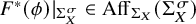 $F^\ast (\phi )\vert _{\Sigma _X^\sigma }\in \operatorname {\mathrm {Aff}}_{\Sigma _X}(\Sigma ^\sigma _X)$
. After potentially restricting
$F^\ast (\phi )\vert _{\Sigma _X^\sigma }\in \operatorname {\mathrm {Aff}}_{\Sigma _X}(\Sigma ^\sigma _X)$
. After potentially restricting
 $\phi $
to the star of a cone containing
$\phi $
to the star of a cone containing
 $\tau $
, we may assume by Lemma 3.2 that
$\tau $
, we may assume by Lemma 3.2 that
 $F(\sigma ^\diamond )\subseteq \tau ^\diamond $
. Then the morphism f maps
$F(\sigma ^\diamond )\subseteq \tau ^\diamond $
. Then the morphism f maps
 $V(\sigma )$
into
$V(\sigma )$
into
 $V(\tau )$
and thus induces a morphism
$V(\tau )$
and thus induces a morphism
 $f\vert _{V(\sigma )}\colon V(\sigma )\to V(\tau )$
. We have
$f\vert _{V(\sigma )}\colon V(\sigma )\to V(\tau )$
. We have
 $$ \begin{align} \mathcal O_{X_\sigma}(F^*(\phi))\vert_{V(\sigma)} \cong \left(f\vert_{X_\sigma}^* \mathcal O_{Y_\tau}(\phi)\right)\vert_{V(\sigma)} \cong f\vert_{V(\sigma)}^* \left( \mathcal O_{Y_\tau}(\phi)\vert_{V(\tau)} \right) \cong f\vert_{V(\sigma)}^* \left(\mathcal O_{V(\tau)}\right)\cong \mathcal O_{V(\sigma)} , \end{align} $$
where the second to last isomorphism follows from
 $\phi $
being affine. Hence
$\phi $
being affine. Hence
 $F^\ast (\phi )$
is affine in a neighborhood of
$F^\ast (\phi )$
is affine in a neighborhood of
 $\sigma $
.
$\sigma $
.
Remark 3.6. In Proposition 3.5, the assumption that f is a dominant toroidal morphism is too strong. All that is needed is that f defines a morphism of log schemes, that is that
 $f(X_0)\subseteq Y_0$
.
$f(X_0)\subseteq Y_0$
.
In the proof of the invariance of the affine structure under modifications, we use the following lemma.
Lemma 3.7. Let
 $f\colon X\to Y$
be a log modification, let
$f\colon X\to Y$
be a log modification, let
 $\tau \in \Sigma _X$
, and let
$\tau \in \Sigma _X$
, and let
 $\sigma \in \Sigma _Y$
be the unique cone with
$\sigma \in \Sigma _Y$
be the unique cone with
 $\tau ^\diamond \subseteq \sigma ^\diamond $
. If
$\tau ^\diamond \subseteq \sigma ^\diamond $
. If
 $\phi \in {\mathrm {sPL}}_{ \Sigma _Y}(\Sigma _Y^\sigma )$
is a piecewise linear function which restricts to an affine function
$\phi \in {\mathrm {sPL}}_{ \Sigma _Y}(\Sigma _Y^\sigma )$
is a piecewise linear function which restricts to an affine function
 $\phi \vert _{\Sigma _X^\tau }\in \operatorname {\mathrm {Aff}}_{\Sigma _X}(\Sigma _X^\tau )$
, then we have
$\phi \vert _{\Sigma _X^\tau }\in \operatorname {\mathrm {Aff}}_{\Sigma _X}(\Sigma _X^\tau )$
, then we have
 $\phi \in \operatorname {\mathrm {Aff}}_{\Sigma _Y}(\Sigma _Y^\sigma )$
.
$\phi \in \operatorname {\mathrm {Aff}}_{\Sigma _Y}(\Sigma _Y^\sigma )$
.
Proof. Let
 $\theta \in \Sigma _X$
be an inclusion-maximal cone with
$\theta \in \Sigma _X$
be an inclusion-maximal cone with
 $\tau \subseteq \theta \subseteq \sigma $
, note that
$\tau \subseteq \theta \subseteq \sigma $
, note that
 $\theta $
and
$\theta $
and
 $\sigma $
have the same dimension. The induced morphism
$\sigma $
have the same dimension. The induced morphism
 $\Sigma _X^\theta /\theta \to \Sigma _Y^\sigma /\sigma $
is a subdivision, and the corresponding logarithmic modification agrees with the restriction
$\Sigma _X^\theta /\theta \to \Sigma _Y^\sigma /\sigma $
is a subdivision, and the corresponding logarithmic modification agrees with the restriction
 $f_\theta := f\vert _{V(\theta )} \colon V(\theta )\to V(\sigma )$
. By Corollary 3.3, the function
$f_\theta := f\vert _{V(\theta )} \colon V(\theta )\to V(\sigma )$
. By Corollary 3.3, the function
 $\phi \vert _{\Sigma _X^\theta }$
is affine at
$\phi \vert _{\Sigma _X^\theta }$
is affine at
 $\theta $
and hence
$\theta $
and hence
 $$ \begin{align} \mathcal O_{V(\theta)}=\mathcal O_{X_\theta}(\phi\vert_{\Sigma_X^\theta})\vert_{V(\theta)} \cong f_\theta^*\left(\mathcal O_{Y_\sigma}(\phi)\vert_{V(\sigma)} \right) \end{align} $$
Taking first Chern classes and using the projection formula, we conclude that
 $$ \begin{align} \mathcal O_{Y_\sigma}(\phi)\vert_{V(\sigma)} \cong \mathcal O_{V(\sigma)} , \end{align} $$
which is equivalent to
 $\phi \in \operatorname {\mathrm {Aff}}_{\Sigma _Y}(\Sigma _Y^\sigma )$
.
$\phi \in \operatorname {\mathrm {Aff}}_{\Sigma _Y}(\Sigma _Y^\sigma )$
.
Proposition 3.8. If
 $f: X\to Y$
is a log modification then the induced morphism
$f: X\to Y$
is a log modification then the induced morphism
 $$ \begin{align} F \colon \vert \Sigma_X\vert\to \vert \Sigma_Y\vert \end{align} $$
is an isomorphism of tropical spaces.
Proof. Since f is a log modification, we know F is a bijective function, and by Proposition 3.5 affine functions pull-back to affine functions. It remains to show that any affine function on
 $\Sigma _X$
can be obtained by pull-back from an affine function of
$\Sigma _X$
can be obtained by pull-back from an affine function of
 $\Sigma _Y$
. Let
$\Sigma _Y$
. Let
 $\tau \in \Sigma _X$
and let
$\tau \in \Sigma _X$
and let
 $\sigma \in \Sigma _Y$
be the unique cone with
$\sigma \in \Sigma _Y$
be the unique cone with
 $\tau ^\diamond \subseteq \sigma ^\diamond $
. We must prove that every function
$\tau ^\diamond \subseteq \sigma ^\diamond $
. We must prove that every function
 $\phi \in \operatorname {\mathrm {Aff}}_{ \Sigma _X}( \Sigma _X^\tau )$
is the restriction of a function in
$\phi \in \operatorname {\mathrm {Aff}}_{ \Sigma _X}( \Sigma _X^\tau )$
is the restriction of a function in
 $\operatorname {\mathrm {Aff}}_{\Sigma _Y}( \Sigma _Y^\sigma )$
.
$\operatorname {\mathrm {Aff}}_{\Sigma _Y}( \Sigma _Y^\sigma )$
.
The setup used in showing that a function
 $\phi \in \operatorname {\mathrm {Aff}}_{ \Sigma _X}( \Sigma _X^\tau )$
is the restriction of a function in
$\phi \in \operatorname {\mathrm {Aff}}_{ \Sigma _X}( \Sigma _X^\tau )$
is the restriction of a function in
 $\operatorname {\mathrm {Aff}}_{\Sigma _Y}( \Sigma _Y^\sigma )$
. The key point is that the map
$\operatorname {\mathrm {Aff}}_{\Sigma _Y}( \Sigma _Y^\sigma )$
. The key point is that the map
 $f_\gamma $
is a
$f_\gamma $
is a
 $\mathbb {P}^1$
bundle. In the illustration we draw
$\mathbb {P}^1$
bundle. In the illustration we draw
 $\theta = \sigma $
for lack of dimensions:
$\theta = \sigma $
for lack of dimensions:
 $\sigma $
is the minimal cone of
$\sigma $
is the minimal cone of
 $\Sigma _Y$
containing
$\Sigma _Y$
containing
 $\tau $
, and
$\tau $
, and
 $\theta $
a maximal cone with such property.
$\theta $
a maximal cone with such property.

First we show that
 $\phi $
is the restriction of a function in
$\phi $
is the restriction of a function in
 ${\mathrm {sPL}}_{ \Sigma _Y}(\Sigma _Y^\sigma )$
, see Figure 2 for the setup. Let
${\mathrm {sPL}}_{ \Sigma _Y}(\Sigma _Y^\sigma )$
, see Figure 2 for the setup. Let
 $\theta \in \Sigma _Y$
be a maximal cone containing
$\theta \in \Sigma _Y$
be a maximal cone containing
 $\sigma $
and let
$\sigma $
and let
 $\delta \in \Sigma _X$
be a maximal cone of
$\delta \in \Sigma _X$
be a maximal cone of
 $ \Sigma _X$
with
$ \Sigma _X$
with
 $\tau \subseteq \delta \subseteq \theta $
. Since the cones
$\tau \subseteq \delta \subseteq \theta $
. Since the cones
 $\delta $
and
$\delta $
and
 $\theta $
have the same dimension, the restriction
$\theta $
have the same dimension, the restriction
 $\phi \vert _\delta $
extends uniquely to a linear function
$\phi \vert _\delta $
extends uniquely to a linear function
 $m_\theta ^\delta $
on the cone
$m_\theta ^\delta $
on the cone
 $\theta $
. We now show that this function does not depend on the choice of
$\theta $
. We now show that this function does not depend on the choice of
 $\delta $
. Let
$\delta $
. Let
 $\delta '\in \Sigma _X$
be a second maximal cone with
$\delta '\in \Sigma _X$
be a second maximal cone with
 $\tau \subseteq \delta '\subseteq \theta $
. Because
$\tau \subseteq \delta '\subseteq \theta $
. Because
 $\delta $
can be reached from
$\delta $
can be reached from
 $\delta '$
by passing through codimension-
$\delta '$
by passing through codimension-
 $1$
cones of
$1$
cones of
 $ \Sigma _X$
that contain
$ \Sigma _X$
that contain
 $\tau $
and are contained in
$\tau $
and are contained in
 $\theta $
, we may assume that
$\theta $
, we may assume that
 $\delta $
and
$\delta $
and
 $\delta '$
are adjacent cones, and
$\delta '$
are adjacent cones, and ![]() has codimension
has codimension
 $1$
. Let
$1$
. Let
 $\varphi =\phi \vert _{\Sigma _X^\gamma }-m_\theta ^\delta \vert _{\Sigma _X^\gamma }$
. Then
$\varphi =\phi \vert _{\Sigma _X^\gamma }-m_\theta ^\delta \vert _{\Sigma _X^\gamma }$
. Then
 $$ \begin{align} \mathcal O_{X_\gamma}(\phi\vert_{\Sigma_X^\gamma}) \cong \mathcal O_{X_\gamma}(\varphi) \otimes f\vert_{X_\gamma}^* \mathcal O_{Y_\theta}(m_\theta^\delta) . \end{align} $$
Denote by
 $f_\gamma \colon V(\gamma )\to V(\theta )$
the restriction of f. Restricting (3.13) to
$f_\gamma \colon V(\gamma )\to V(\theta )$
the restriction of f. Restricting (3.13) to
 $V(\gamma )$
and using the hypothesis of
$V(\gamma )$
and using the hypothesis of
 $\phi $
being affine we obtain
$\phi $
being affine we obtain
 $$ \begin{align} \mathcal O_{V(\gamma)} \cong \mathcal O_{X_\gamma}(\varphi)\vert_{V(\gamma)} \otimes f_\gamma^* \mathcal O_{Y_\theta}(m_\theta^\delta)\vert_{V(\theta)} . \end{align} $$
The function
 $\varphi $
vanishes on
$\varphi $
vanishes on
 $\gamma $
and therefore induces a function
$\gamma $
and therefore induces a function
 $\overline \varphi $
on the star
$\overline \varphi $
on the star
 $ \Sigma _X^\gamma /\gamma =\Sigma _{V(\gamma )}$
. Since
$ \Sigma _X^\gamma /\gamma =\Sigma _{V(\gamma )}$
. Since
 $\gamma $
has codimension
$\gamma $
has codimension
 $1$
in
$1$
in
 $\theta $
, the star
$\theta $
, the star
 $\Sigma _X^\gamma /\gamma $
is a union of two rays, corresponding to the divisors
$\Sigma _X^\gamma /\gamma $
is a union of two rays, corresponding to the divisors
 $V(\delta )$
and
$V(\delta )$
and
 $V(\delta ')$
in
$V(\delta ')$
in
 $V(\gamma )$
, which both map isomorphically onto
$V(\gamma )$
, which both map isomorphically onto
 $V(\theta )$
. That makes
$V(\theta )$
. That makes
 $f_\gamma $
a
$f_\gamma $
a ![]() -bundle on
-bundle on
 $V(\theta )$
with two distinct sections. The function
$V(\theta )$
with two distinct sections. The function
 $\overline \varphi $
has slope
$\overline \varphi $
has slope
 $0$
on the ray corresponding to
$0$
on the ray corresponding to
 $V(\delta )$
, we show that it must have slope
$V(\delta )$
, we show that it must have slope
 $0$
along the other ray as well. If k is the slope of
$0$
along the other ray as well. If k is the slope of
 $\overline \varphi $
on the ray corresponding to
$\overline \varphi $
on the ray corresponding to
 $V(\delta ')$
, then
$V(\delta ')$
, then
 $$ \begin{align} \mathcal O_{X_\gamma}(\varphi)\vert_{V(\gamma)} \cong \mathcal O_{V(\gamma)}(\overline \varphi) \cong \mathcal O_{V(\gamma)}(V(\delta'))^{\otimes k} \end{align} $$
and hence (3.14) gives
 $$ \begin{align} \mathcal O_{V(\gamma)} \cong \mathcal O_{V(\gamma)}(V(\delta'))^{\otimes k} \otimes f_\gamma^* \mathcal O_{Y_\theta}(m_\theta^\delta)\vert_{V(\theta)} . \end{align} $$
Since ![]() by virtue of the projective bundle formula, it follows that
by virtue of the projective bundle formula, it follows that
 $k=0$
, that is,
$k=0$
, that is,
 $\varphi \vert _{\delta '}=0$
. From this it follows immediately that
$\varphi \vert _{\delta '}=0$
. From this it follows immediately that
 $m^\delta _\theta =m^{\delta '}_\theta $
.
$m^\delta _\theta =m^{\delta '}_\theta $
.
Illustration for the second part of the argument in Proposition 3.8. Here by lack of dimensions we have drawn
 $\sigma = \gamma $
. Observe that
$\sigma = \gamma $
. Observe that
 $\tilde {\gamma } \subset \gamma $
, and the cones
$\tilde {\gamma } \subset \gamma $
, and the cones
 $\theta $
and
$\theta $
and
 $\theta '$
are the two-dimensional triangles bounded by the black edges.
$\theta '$
are the two-dimensional triangles bounded by the black edges.

For
 $\theta \in \Sigma _Y$
a maximal cone containing
$\theta \in \Sigma _Y$
a maximal cone containing
 $\sigma $
we can now define
$\sigma $
we can now define
 $m_\theta =m^\delta _\theta $
for some maximal cone
$m_\theta =m^\delta _\theta $
for some maximal cone
 $\delta \in \Sigma _X$
with
$\delta \in \Sigma _X$
with
 $\tau \subseteq \delta \subseteq \theta $
; this is independent of the choice of
$\tau \subseteq \delta \subseteq \theta $
; this is independent of the choice of
 $\delta $
. Given a second maximal cone
$\delta $
. Given a second maximal cone
 $\theta '\in \Sigma _Y$
containing
$\theta '\in \Sigma _Y$
containing
 $\sigma $
intersecting
$\sigma $
intersecting
 $\theta $
in
$\theta $
in ![]() , we claim that
, we claim that
 $$ \begin{align} m_\theta\vert_\gamma=m_\theta'\vert_\gamma . \end{align} $$
Referring to Figure 3, if
 $\widetilde \gamma \in \Sigma _X$
is a maximal cone in
$\widetilde \gamma \in \Sigma _X$
is a maximal cone in
 $\gamma $
containing
$\gamma $
containing
 $\tau $
, then there exist maximal cones
$\tau $
, then there exist maximal cones
 $\delta ,\delta '\in \Sigma _X$
containing
$\delta ,\delta '\in \Sigma _X$
containing
 $\widetilde \gamma $
with
$\widetilde \gamma $
with
 $\delta \subseteq \theta $
and
$\delta \subseteq \theta $
and
 $\delta '\subseteq \theta '$
. Then we have
$\delta '\subseteq \theta '$
. Then we have
 $$ \begin{align} m_\theta\vert_{\widetilde\gamma}=m_\theta^\delta\vert_{\widetilde\gamma}=\phi\vert_{\widetilde\gamma}=m_{\theta'}^{\delta'}\vert_{\widetilde\gamma}=m_{\theta'}\vert_{\widetilde\gamma} . \end{align} $$
As
 $\widetilde \gamma $
is full-dimensional in
$\widetilde \gamma $
is full-dimensional in
 $\gamma $
, this shows the desired equality. We conclude that the functions
$\gamma $
, this shows the desired equality. We conclude that the functions
 $m_\theta $
glue to give a function
$m_\theta $
glue to give a function
 $\widetilde \phi \in {\mathrm {sPL}}_{ \Sigma _Y}(\Sigma _Y^\sigma )$
, and by construction we have
$\widetilde \phi \in {\mathrm {sPL}}_{ \Sigma _Y}(\Sigma _Y^\sigma )$
, and by construction we have
 $\widetilde \phi \vert _{\Sigma _X^\tau }=\phi $
. By Lemma 3.7, we have
$\widetilde \phi \vert _{\Sigma _X^\tau }=\phi $
. By Lemma 3.7, we have
 $\widetilde \phi \in \operatorname {\mathrm {Aff}}_{ \Sigma _Y}(\Sigma _Y^\sigma )$
, completing the proof.
$\widetilde \phi \in \operatorname {\mathrm {Aff}}_{ \Sigma _Y}(\Sigma _Y^\sigma )$
, completing the proof.
Remark 3.9. Proposition 3.8 allows us to remove the hypothesis that the boundary of X does not have strata with self intersections or pairs of strata with multiple intersections. Hypothesis
 $(\ast )$
may always be achieved via some log modification, for example, by subdividing barycentrically the generalized cone complex
$(\ast )$
may always be achieved via some log modification, for example, by subdividing barycentrically the generalized cone complex
 $\Sigma _X$
of the original space. We then define the affine structure on the tropicalization as the affine structure on any refinement where
$\Sigma _X$
of the original space. We then define the affine structure on the tropicalization as the affine structure on any refinement where
 $(\ast )$
holds; by Proposition 3.8, it is a well defined affine structure on
$(\ast )$
holds; by Proposition 3.8, it is a well defined affine structure on
 $\Sigma _X$
.
$\Sigma _X$
.
3.2 The affine structure at infinity
In this section, we extend the previous constructions to the context of extended cone complexes. Given a cone complex
 $\Sigma $
, its extended cone complex is set-theoretically described as a disjoint union of quotients of cone complexes indexed by the cones of
$\Sigma $
, its extended cone complex is set-theoretically described as a disjoint union of quotients of cone complexes indexed by the cones of
 $\Sigma $
:
$\Sigma $
:
 $$ \begin{align} \overline\Sigma = \bigsqcup_{\sigma\in \Sigma}\Sigma^\sigma/\sigma . \end{align} $$
Observe that if
 $0_\Sigma $
is the cone point of
$0_\Sigma $
is the cone point of
 $\Sigma $
, then
$\Sigma $
, then
 $\Sigma ^{0_\Sigma }/0_\Sigma = \Sigma $
. We call sets of the form
$\Sigma ^{0_\Sigma }/0_\Sigma = \Sigma $
. We call sets of the form
 $\sigma /\tau \subseteq \overline \Sigma $
for some
$\sigma /\tau \subseteq \overline \Sigma $
for some
 $\sigma \supseteq \tau \in \Sigma $
the cells of the extended cone complex. The open star of a cell of an extended cone complex is
$\sigma \supseteq \tau \in \Sigma $
the cells of the extended cone complex. The open star of a cell of an extended cone complex is
 $$ \begin{align} \overline\Sigma^{\sigma/\tau}= \bigcup_{ \substack{\scriptscriptstyle\tilde\sigma \supseteq \sigma\\ \scriptscriptstyle\tilde\tau \subseteq \tau} } (\tilde\sigma/\tilde\tau)^\diamond . \end{align} $$
Taking
 $\tau = 0_\Sigma $
, (3.20) agrees with the earlier notion of open star of a cone in a cone complex (3.2). We will denote by
$\tau = 0_\Sigma $
, (3.20) agrees with the earlier notion of open star of a cone in a cone complex (3.2). We will denote by
 ${\mathrm {sPL}}(\overline \Sigma ^{\sigma /\tau })$
the subgroup of
${\mathrm {sPL}}(\overline \Sigma ^{\sigma /\tau })$
the subgroup of
 ${\mathrm {sPL}}(\Sigma ^\sigma )$
consisting of those functions whose continuous extensions to
${\mathrm {sPL}}(\Sigma ^\sigma )$
consisting of those functions whose continuous extensions to
 $\overline {\Sigma ^\sigma }$
are constant on
$\overline {\Sigma ^\sigma }$
are constant on
 $\tau $
. Equivalently, the functions in
$\tau $
. Equivalently, the functions in
 ${\mathrm {sPL}}(\overline \Sigma ^{\sigma /\tau })$
are precisely those functions in
${\mathrm {sPL}}(\overline \Sigma ^{\sigma /\tau })$
are precisely those functions in
 ${\mathrm {sPL}}(\Sigma ^\sigma )$
that extend continuously to
${\mathrm {sPL}}(\Sigma ^\sigma )$
that extend continuously to
 $\overline \Sigma ^{\sigma /\tau }$
.
$\overline \Sigma ^{\sigma /\tau }$
.
Definition 3.10. Let X be a toroidal variety, and let
 $\overline {\Sigma }_X$
denote the extended cone complex associated to X. We extend the affine structure on
$\overline {\Sigma }_X$
denote the extended cone complex associated to X. We extend the affine structure on
 $\Sigma _X$
to
$\Sigma _X$
to
 $\overline {\Sigma }_X$
by defining
$\overline {\Sigma }_X$
by defining
 $$ \begin{align} \operatorname{\mathrm{Aff}}_{\overline\Sigma_X}= \iota_*\operatorname{\mathrm{Aff}}_{\Sigma_X}\cap {\mathrm{PL}}^{\mathrm{fin}}_{\overline\Sigma_X} , \end{align} $$
where
 $\iota \colon \Sigma _X\to \overline \Sigma _X$
denotes the inclusion, and the intersection is taken in
$\iota \colon \Sigma _X\to \overline \Sigma _X$
denotes the inclusion, and the intersection is taken in
 $\iota _*{\mathrm {PL}}^{\mathrm {fin}}_{\Sigma _X}$
. In other words, the affine functions on
$\iota _*{\mathrm {PL}}^{\mathrm {fin}}_{\Sigma _X}$
. In other words, the affine functions on
 $\overline \Sigma _X$
are precisely the continuous extension of the affine functions on
$\overline \Sigma _X$
are precisely the continuous extension of the affine functions on
 $\Sigma _X$
.
$\Sigma _X$
.
An important feature of extended tropicalization is that at infinity one can witness a stratification by the
 ${\Sigma }^\sigma /\sigma $
’s, which is parallel (rather than opposite) to the original toroidal stratification. The idea is that the geometry at infinity in the direction of
${\Sigma }^\sigma /\sigma $
’s, which is parallel (rather than opposite) to the original toroidal stratification. The idea is that the geometry at infinity in the direction of
 $\tau $
should reflect the geometry of
$\tau $
should reflect the geometry of
 $V(\tau )$
. For a cell at infinity of the the form
$V(\tau )$
. For a cell at infinity of the the form
 $\sigma /\tau $
, we define
$\sigma /\tau $
, we define
 $V(\sigma /\tau )=V(\sigma )$
, which we think of as a closed stratum inside
$V(\sigma /\tau )=V(\sigma )$
, which we think of as a closed stratum inside
 $V(\tau )$
. We show that affine structures are compatible with this perspective.
$V(\tau )$
. We show that affine structures are compatible with this perspective.
Lemma 3.11. Let
 $\sigma \in \Sigma _X$
, let
$\sigma \in \Sigma _X$
, let
 $\tau $
be a face of
$\tau $
be a face of
 $\sigma $
, and let
$\sigma $
, and let
 $\phi \in {\mathrm {sPL}}(\Sigma _X^\sigma )$
such that
$\phi \in {\mathrm {sPL}}(\Sigma _X^\sigma )$
such that
 $\phi \vert _\tau $
is constant. Denote by
$\phi \vert _\tau $
is constant. Denote by
 $\pi _\tau \colon \Sigma _X^\tau \to \Sigma _X^\tau /\tau $
the projection and by
$\pi _\tau \colon \Sigma _X^\tau \to \Sigma _X^\tau /\tau $
the projection and by
 $\chi $
the unique piecewise linear function on
$\chi $
the unique piecewise linear function on
 $(\Sigma _X^\tau /\tau )^{\sigma /\tau }$
such that
$(\Sigma _X^\tau /\tau )^{\sigma /\tau }$
such that
 $\phi =\pi ^*_\tau \chi $
. Then
$\phi =\pi ^*_\tau \chi $
. Then
 $\phi $
is affine at
$\phi $
is affine at
 $\sigma $
if and only if
$\sigma $
if and only if
 $\chi $
is affine at
$\chi $
is affine at
 $\sigma /\tau $
in the affine structure on
$\sigma /\tau $
in the affine structure on
 $\Sigma _X^\tau /\tau $
defined using the natural identification
$\Sigma _X^\tau /\tau $
defined using the natural identification
 $\Sigma _X^\tau /\tau \cong \Sigma _{V(\tau )}$
.
$\Sigma _X^\tau /\tau \cong \Sigma _{V(\tau )}$
.
Proof. As
 $\phi $
is constant on
$\phi $
is constant on
 $\tau $
, the support of the Cartier divisor
$\tau $
, the support of the Cartier divisor
 $D_{X_\sigma }(\phi )$
is does not contain
$D_{X_\sigma }(\phi )$
is does not contain
 $V(\tau )$
, hence its restriction to
$V(\tau )$
, hence its restriction to
 $V(\tau )$
is transversal:
$V(\tau )$
is transversal:
 $$ \begin{align} D_{X_\sigma}(\phi)\vert_{V(\tau)_{\sigma/\tau}}=D_{V(\tau)_{\sigma/\tau}}(\chi) . \end{align} $$
It follows that
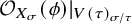 $\mathcal O_{X_\sigma }(\phi )\vert _{V(\tau )_{\sigma /\tau }}$
agrees with
$\mathcal O_{X_\sigma }(\phi )\vert _{V(\tau )_{\sigma /\tau }}$
agrees with
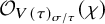 $\mathcal O_{V(\tau )_{\sigma /\tau }}(\chi )$
, and, in particular, their restriction to
$\mathcal O_{V(\tau )_{\sigma /\tau }}(\chi )$
, and, in particular, their restriction to
 $V(\sigma )$
agree, from which the assertion follows immediately.
$V(\sigma )$
agree, from which the assertion follows immediately.
Proposition 3.12. Let X be a toroidal variety with tropicalization
 $\Sigma _X$
, and let
$\Sigma _X$
, and let
 $\tau \in \Sigma _X$
. With the natural identification
$\tau \in \Sigma _X$
. With the natural identification
 $ \Sigma _X^\tau /\tau = \Sigma _{V(\tau )}$
, we have an isomorphism
$ \Sigma _X^\tau /\tau = \Sigma _{V(\tau )}$
, we have an isomorphism
 $$ \begin{align} \operatorname{\mathrm{Aff}}_{\overline\Sigma_X}\vert_{ \Sigma_X^\tau/\tau} \cong \operatorname{\mathrm{Aff}}_{\Sigma_{V(\tau)}} \end{align} $$
Proof. By definition, the affine structure
 $\operatorname {\mathrm {Aff}}_{\Sigma _X}$
is generated by strict piecewise linear functions. Such a function extends to a finite piecewise linear function in a neighborhood of a cell
$\operatorname {\mathrm {Aff}}_{\Sigma _X}$
is generated by strict piecewise linear functions. Such a function extends to a finite piecewise linear function in a neighborhood of a cell
 $\sigma /\tau \subseteq \overline \Sigma _X$
if and only if it is constant on
$\sigma /\tau \subseteq \overline \Sigma _X$
if and only if it is constant on
 $\tau $
. The assertion now follows from Lemma 3.11.
$\tau $
. The assertion now follows from Lemma 3.11.
Corollary 3.13. Let
 $f: X\to Y$
be a (not necessarily dominant) toroidal morphism of toroidal varieties. Then the natural piecewise linear map
$f: X\to Y$
be a (not necessarily dominant) toroidal morphism of toroidal varieties. Then the natural piecewise linear map
 $$ \begin{align} {\mathtt{Trop}}(f) \colon \vert \overline \Sigma_X\vert\to \vert \overline \Sigma_Y\vert \end{align} $$
is a morphism of tropical spaces.
3.3 Affine structures on families of curves
We apply the constructions in Section 3.1 to families of curves and their tropicalizations. We first observe, in what seems like a groundhog day moment but is a necessary verification, that in genus zero the affine structures we obtain from tropicalization agree with those from [Reference Cavalieri, Gross and Markwig6] and with those obtained from any prior incarnation of
 $\mathcal M_{0,n}^{\mathtt {trop}}$
. Next we study the tropicalization of families of curves of arbitrary genus, and observe that while tropicalization gives a map of TPL-spaces with affine structures, this is not always a family of tropical curves with affine structures in the sense of [Reference Cavalieri, Gross and Markwig6]. However we identify combinatorial conditions describing a locus where the affine structures agree. We begin with some technical definitions that are useful in developing these ideas.
$\mathcal M_{0,n}^{\mathtt {trop}}$
. Next we study the tropicalization of families of curves of arbitrary genus, and observe that while tropicalization gives a map of TPL-spaces with affine structures, this is not always a family of tropical curves with affine structures in the sense of [Reference Cavalieri, Gross and Markwig6]. However we identify combinatorial conditions describing a locus where the affine structures agree. We begin with some technical definitions that are useful in developing these ideas.
Definition 3.14. Let
 $\Sigma $
be a pure-dimensional cone complex, let
$\Sigma $
be a pure-dimensional cone complex, let
 $\sigma \in \Sigma $
, and let
$\sigma \in \Sigma $
, and let
 $H^\sigma $
be a subgroup of
$H^\sigma $
be a subgroup of
 ${\mathrm {sPL}}(\Sigma ^\sigma )$
such that
${\mathrm {sPL}}(\Sigma ^\sigma )$
such that
 $[\Sigma ^\sigma ]$
(the weight on
$[\Sigma ^\sigma ]$
(the weight on
 $\Sigma ^\sigma $
which is
$\Sigma ^\sigma $
which is
 $1$
on all top-dimensional cones) is balanced in the affine structure induced by
$1$
on all top-dimensional cones) is balanced in the affine structure induced by
 $H^\sigma $
. Let
$H^\sigma $
. Let
 ${\mathrm {CP}}_{H^\sigma }(\Sigma ^\sigma )$
denote the subgroup of
${\mathrm {CP}}_{H^\sigma }(\Sigma ^\sigma )$
denote the subgroup of
 ${\mathrm {sPL}}(\Sigma ^\sigma )$
consisting of those piecewise linear functions
${\mathrm {sPL}}(\Sigma ^\sigma )$
consisting of those piecewise linear functions
 $\phi $
for which on every cone
$\phi $
for which on every cone
 $\delta $
of
$\delta $
of
 $\Sigma ^\sigma $
there exists a function
$\Sigma ^\sigma $
there exists a function
 $h\in H^\sigma $
with
$h\in H^\sigma $
with
 $\phi \vert _\delta =h\vert _\delta $
. We define the closure
$\phi \vert _\delta =h\vert _\delta $
. We define the closure
 $\overline {H^\sigma }$
of
$\overline {H^\sigma }$
of
 $H^\sigma $
as
$H^\sigma $
as
 $$ \begin{align} \overline{H^\sigma}=\{\phi\in {\mathrm{CP}}_{H^\sigma}(\Sigma^\sigma) \mid \phi\cdot [\Sigma^\sigma]=0 \} \end{align} $$
and say that
 $H^\sigma $
is normal if
$H^\sigma $
is normal if
 $H^\sigma =\overline {H^\sigma }$
. When no superscript is added, we assume that we are choosing
$H^\sigma =\overline {H^\sigma }$
. When no superscript is added, we assume that we are choosing
 $\sigma $
to be the cone point
$\sigma $
to be the cone point
 $0_\Sigma $
.
$0_\Sigma $
.
Example 3.15. Consider a cone complex
 $\Sigma $
with one vertex and four rays denoted
$\Sigma $
with one vertex and four rays denoted
 $\rho _{i}$
, for
$\rho _{i}$
, for
 $i = 1,\ldots , 4$
. Denote by
$i = 1,\ldots , 4$
. Denote by
 $\varphi _{i}$
the piecewise linear function with slope one along
$\varphi _{i}$
the piecewise linear function with slope one along
 $\rho _i$
and zero along all other rays. For
$\rho _i$
and zero along all other rays. For
 $\sigma $
equal to the vertex
$\sigma $
equal to the vertex
 $0_\Sigma $
, if we choose
$0_\Sigma $
, if we choose
then
 $\Sigma ^\sigma = \Sigma $
is balanced at
$\Sigma ^\sigma = \Sigma $
is balanced at
 $\sigma $
in the affine structure induced by H. In this case
$\sigma $
in the affine structure induced by H. In this case
 ${\mathrm {CP}}_H(\Sigma ) = {\mathrm {sPL}}(\Sigma )$
, as one can find on each ray a function in H with any given integral slope.
${\mathrm {CP}}_H(\Sigma ) = {\mathrm {sPL}}(\Sigma )$
, as one can find on each ray a function in H with any given integral slope.
The piecewise linear function
 $\varphi _3-\varphi _4$
belongs to
$\varphi _3-\varphi _4$
belongs to
 $\overline {H}\smallsetminus H$
, thus showing that H is not normal. One can verify that adding this function one spans all of
$\overline {H}\smallsetminus H$
, thus showing that H is not normal. One can verify that adding this function one spans all of
 $\overline {H}$
, thus
$\overline {H}$
, thus
See Figure 4 for a geometric illustration of this example.
In the next proposition, we show that
 $\overline {H^\sigma }$
is the largest subgroup of
$\overline {H^\sigma }$
is the largest subgroup of
 ${\mathrm {CP}}_{H^\sigma }(\Sigma ^\sigma )$
containing
${\mathrm {CP}}_{H^\sigma }(\Sigma ^\sigma )$
containing
 $H^\sigma $
in which
$H^\sigma $
in which
 $\Sigma ^\sigma $
is balanced at
$\Sigma ^\sigma $
is balanced at
 $\sigma $
.
$\sigma $
.
Proposition 3.16. Let X be a toroidal variety with associated cone complex
 $\Sigma _X$
, let
$\Sigma _X$
, let
 $\sigma \in \Sigma _X$
, and let
$\sigma \in \Sigma _X$
, and let
 $H^\sigma \subseteq \operatorname {\mathrm {Aff}}_{\Sigma _X}(\Sigma _X^\sigma )$
be a subgroup such that
$H^\sigma \subseteq \operatorname {\mathrm {Aff}}_{\Sigma _X}(\Sigma _X^\sigma )$
be a subgroup such that
 $[\Sigma _X^\sigma ]$
is balanced. Then we have
$[\Sigma _X^\sigma ]$
is balanced. Then we have
 $$ \begin{align} \operatorname{\mathrm{Aff}}_{\Sigma_X}(\Sigma_X^\sigma)\cap {\mathrm{CP}}_{H^\sigma}(\Sigma_X^\sigma)\subseteq \overline{H^\sigma} . \end{align} $$
In particular, if
 ${\mathrm {CP}}_{H^\sigma }(\Sigma _X^\sigma )={\mathrm {sPL}}(\Sigma _X^ \sigma )$
, we have
${\mathrm {CP}}_{H^\sigma }(\Sigma _X^\sigma )={\mathrm {sPL}}(\Sigma _X^ \sigma )$
, we have
 $\operatorname {\mathrm {Aff}}_{\Sigma _X}(\Sigma _X^\sigma ) \subseteq \overline {H^\sigma } $
.
$\operatorname {\mathrm {Aff}}_{\Sigma _X}(\Sigma _X^\sigma ) \subseteq \overline {H^\sigma } $
.
Proof. Let
 $\phi \in \operatorname {\mathrm {Aff}}_{\Sigma _X}(\Sigma _X^\sigma )\cap {\mathrm {CP}}_{H^\sigma }(\Sigma _X^\sigma )$
. We will show in Corollary 5.8 that with the affine structure
$\phi \in \operatorname {\mathrm {Aff}}_{\Sigma _X}(\Sigma _X^\sigma )\cap {\mathrm {CP}}_{H^\sigma }(\Sigma _X^\sigma )$
. We will show in Corollary 5.8 that with the affine structure
 $\operatorname {\mathrm {Aff}}_{\Sigma _X}$
, the intersection product
$\operatorname {\mathrm {Aff}}_{\Sigma _X}$
, the intersection product
 $\phi \cdot [\Sigma _X^\sigma ]$
vanishes. Since
$\phi \cdot [\Sigma _X^\sigma ]$
vanishes. Since
 $H^\sigma \subseteq \operatorname {\mathrm {Aff}}_{\Sigma _X}(\Sigma _X^\sigma )$
, we have
$H^\sigma \subseteq \operatorname {\mathrm {Aff}}_{\Sigma _X}(\Sigma _X^\sigma )$
, we have
 $\phi \cdot [\Sigma _X^\sigma ]=0$
even with respect to the affine structure defined by
$\phi \cdot [\Sigma _X^\sigma ]=0$
even with respect to the affine structure defined by
 $H^\sigma $
, that is
$H^\sigma $
, that is
 $\phi \in \overline {H^\sigma }$
.
$\phi \in \overline {H^\sigma }$
.
Theorem 3.17. Via the canonical identification of the underlying cone complexes, the affine structure on
 $\overline \Sigma _{\overline {\mathcal M}_{0,n}}$
agrees with the affine structure on
$\overline \Sigma _{\overline {\mathcal M}_{0,n}}$
agrees with the affine structure on
 $\overline {\mathcal M}_{0,n}^{\mathtt {trop}}$
(as defined in [Reference Cavalieri, Gross and Markwig6, Section 4]).
$\overline {\mathcal M}_{0,n}^{\mathtt {trop}}$
(as defined in [Reference Cavalieri, Gross and Markwig6, Section 4]).
Proof. By Definition 3.10, we have
 $$ \begin{align} \operatorname{\mathrm{Aff}}_{\overline\Sigma_{\overline{\mathcal M}_{0,n}}}=\iota_*\operatorname{\mathrm{Aff}}_{\Sigma_{\overline{\mathcal M}_{0,n}}} \cap {\mathrm{PL}}^{\mathrm{fin}}_{\overline\Sigma_{\overline{\mathcal M}_{0,n}}} , \end{align} $$
where
 $\iota \colon \Sigma _{\overline {\mathcal M}_{0,n}}\to \overline \Sigma _{\overline {\mathcal M}_{0,n}}$
is the inclusion. By [Reference Cavalieri, Gross and Markwig6, Lemma 4.16] we also have
$\iota \colon \Sigma _{\overline {\mathcal M}_{0,n}}\to \overline \Sigma _{\overline {\mathcal M}_{0,n}}$
is the inclusion. By [Reference Cavalieri, Gross and Markwig6, Lemma 4.16] we also have
 $$ \begin{align} \operatorname{\mathrm{Aff}}_{\overline{\mathcal M}_{0,n}^{\mathtt{trop}}}= \kappa_*\operatorname{\mathrm{Aff}}_{\mathcal M_{0,n}^{\mathtt{trop}}}\cap {\mathrm{PL}}^{\mathrm{fin}}_{\overline{\mathcal M}_{0,n}^{\mathtt{trop}}} , \end{align} $$
where
 $\kappa \colon \mathcal M_{0,n}^{\mathtt {trop}}\to \overline {\mathcal M}_{0,n}^{\mathtt {trop}}$
denotes the inclusion. Since
$\kappa \colon \mathcal M_{0,n}^{\mathtt {trop}}\to \overline {\mathcal M}_{0,n}^{\mathtt {trop}}$
denotes the inclusion. Since
 $ {\mathrm {PL}}^{\mathrm {fin}}_{\overline \Sigma _{\overline {\mathcal M}_{0,n}}} \hspace {-.4cm}= \ {\mathrm {PL}}^{\mathrm {fin}}_{\overline {\mathcal M}_{0,n}^{\mathtt {trop}}}$
, it suffices to show that the affine structures on
$ {\mathrm {PL}}^{\mathrm {fin}}_{\overline \Sigma _{\overline {\mathcal M}_{0,n}}} \hspace {-.4cm}= \ {\mathrm {PL}}^{\mathrm {fin}}_{\overline {\mathcal M}_{0,n}^{\mathtt {trop}}}$
, it suffices to show that the affine structures on
 $\Sigma _{\overline {\mathcal M}_{0,n}}$
and
$\Sigma _{\overline {\mathcal M}_{0,n}}$
and
 $\mathcal M_{0,n}^{\mathtt {trop}}$
coincide.
$\mathcal M_{0,n}^{\mathtt {trop}}$
coincide.
The primitive ray generators for the cone complex
 $\Sigma $
, depicted in red, are embedded into
$\Sigma $
, depicted in red, are embedded into ![]() via the chosen generators of H, and into
via the chosen generators of H, and into ![]() via the generators of
via the generators of
 $\overline {H}$
. The two balanced fans are related by a linear function. The failure of normality of H detects the fact that the embedding of
$\overline {H}$
. The two balanced fans are related by a linear function. The failure of normality of H detects the fact that the embedding of
 $\Sigma $
as a plane balanced fan is not as linearly independent as possible.
$\Sigma $
as a plane balanced fan is not as linearly independent as possible.

By [Reference Cavalieri, Gross and Markwig6, Theorem 4.32], affine functions on
 $\mathcal M_{0,n}^{\mathtt {trop}}$
are given by cross ratios [Reference Cavalieri, Gross and Markwig6, Definition 4.8]. We first show that the tropicalization of a cross ratio on
$\mathcal M_{0,n}^{\mathtt {trop}}$
are given by cross ratios [Reference Cavalieri, Gross and Markwig6, Definition 4.8]. We first show that the tropicalization of a cross ratio on
 $\mathcal M_{0,n}$
is a tropical cross ratio. All cross ratios are pull-backs of cross ratios on
$\mathcal M_{0,n}$
is a tropical cross ratio. All cross ratios are pull-backs of cross ratios on
 $\mathcal M_{0,4}$
via the forgetful map, both algebraically and tropically, and tropicalization respects the
$\mathcal M_{0,4}$
via the forgetful map, both algebraically and tropically, and tropicalization respects the
 $S_4$
-action on
$S_4$
-action on
 $\mathcal M_{0,4}$
. Thus, by the functoriality of taking cone complexes of Proposition 3.5, it suffices to show that the cross ratio
$\mathcal M_{0,4}$
. Thus, by the functoriality of taking cone complexes of Proposition 3.5, it suffices to show that the cross ratio
 $(p_1,p_2;p_3,p_4)$
on
$(p_1,p_2;p_3,p_4)$
on
 $\mathcal M_{0,4}$
tropicalizes to a cross ratio. We have
$\mathcal M_{0,4}$
tropicalizes to a cross ratio. We have
 $$ \begin{align} (\infty,0;1, z) = z , \end{align} $$
whose associated divisor is
 $(0)-(\infty )$
. The point
$(0)-(\infty )$
. The point
 $0$
corresponds to the nodal curve
$0$
corresponds to the nodal curve
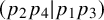 $(p_2p_4 \vert p_1p_3)$
, whereas the point
$(p_2p_4 \vert p_1p_3)$
, whereas the point
 $\infty $
corresponds to the curve
$\infty $
corresponds to the curve
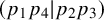 $(p_1p_4\vert p_2p_3)$
. Therefore, the tropicalization of the cross ratio
$(p_1p_4\vert p_2p_3)$
. Therefore, the tropicalization of the cross ratio
 $(p_1,p_2;p_3,p_4)$
is the function with slope
$(p_1,p_2;p_3,p_4)$
is the function with slope
 $1$
on the ray
$1$
on the ray
 $\rho _{(13\vert 24)}$
, slope
$\rho _{(13\vert 24)}$
, slope
 $-1$
on the ray
$-1$
on the ray
 $\rho _{(14\vert 23)}$
, and slope
$\rho _{(14\vert 23)}$
, and slope
 $0$
on the ray
$0$
on the ray
 $\rho _{(12\vert 34)}$
. This is precisely the tropical cross ratio function
$\rho _{(12\vert 34)}$
. This is precisely the tropical cross ratio function
 $\xi _{((1,2),(3,4))}$
corresponding to the primitive vertex cross ratio datum
$\xi _{((1,2),(3,4))}$
corresponding to the primitive vertex cross ratio datum
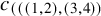 $c_{(((1,2),(3,4))}$
at the unique vertex of the tropical curve in the minimal cone of
$c_{(((1,2),(3,4))}$
at the unique vertex of the tropical curve in the minimal cone of
 $\mathcal M_{0,4}^{\mathtt {trop}}$
.
$\mathcal M_{0,4}^{\mathtt {trop}}$
.
We have shown that the natural identification
 $$ \begin{align} \Sigma_{\overline{\mathcal M}_{0,n}}\to \mathcal M_{0,n}^{\mathtt{trop}} \end{align} $$
is linear. It remains to show that there are not more functions on
 $\Sigma _{\overline {\mathcal M}_{0,n}}$
. The subgroup
$\Sigma _{\overline {\mathcal M}_{0,n}}$
. The subgroup
 $H = \operatorname {\mathrm {Aff}}_{\mathcal M_{0,n}^{\mathtt {trop}}}(\Sigma _{\overline {\mathcal M}_{0,n}})$
is naturally identified with the dual to the integral lattice in
$H = \operatorname {\mathrm {Aff}}_{\mathcal M_{0,n}^{\mathtt {trop}}}(\Sigma _{\overline {\mathcal M}_{0,n}})$
is naturally identified with the dual to the integral lattice in ![]() . Since
. Since
 $\mathcal M_{0,n}^{\mathtt {trop}}$
is a tropical linear space [Reference Maclagan and Sturmfels20, Theorem 6.4.12], we have that
$\mathcal M_{0,n}^{\mathtt {trop}}$
is a tropical linear space [Reference Maclagan and Sturmfels20, Theorem 6.4.12], we have that
 $H = \overline {H}$
by [Reference Francois10, Proposition 4.5]. In addition
$H = \overline {H}$
by [Reference Francois10, Proposition 4.5]. In addition
 ${\mathrm {CP}}_H(\mathcal M_{0,n}^{\mathtt {trop}})={\mathrm {sPL}}(\mathcal M_{0,n}^{\mathtt {trop}})$
, because
${\mathrm {CP}}_H(\mathcal M_{0,n}^{\mathtt {trop}})={\mathrm {sPL}}(\mathcal M_{0,n}^{\mathtt {trop}})$
, because
 $\mathcal M_{0,n}^{\mathtt {trop}}$
is embedded in
$\mathcal M_{0,n}^{\mathtt {trop}}$
is embedded in ![]() by its global linear functions. We can thus apply Proposition 3.16 to conclude that
by its global linear functions. We can thus apply Proposition 3.16 to conclude that
 $\operatorname {\mathrm {Aff}}_{\Sigma _{\overline {\mathcal M}_{0,n}}}(\Sigma _{\overline {\mathcal M}_{0,n}})\subseteq \overline {H} = \operatorname {\mathrm {Aff}}_{\mathcal M_{0,n}^{\mathtt {trop}}}(\Sigma _{\overline {\mathcal M}_{0,n}})$
.
$\operatorname {\mathrm {Aff}}_{\Sigma _{\overline {\mathcal M}_{0,n}}}(\Sigma _{\overline {\mathcal M}_{0,n}})\subseteq \overline {H} = \operatorname {\mathrm {Aff}}_{\mathcal M_{0,n}^{\mathtt {trop}}}(\Sigma _{\overline {\mathcal M}_{0,n}})$
.
Given any cone
 $\sigma \in \mathcal M_{0,n}^{\mathtt {trop}}$
, the same argument applies to
$\sigma \in \mathcal M_{0,n}^{\mathtt {trop}}$
, the same argument applies to
 $\Sigma _{\overline {\mathcal M}_{0,n}}^\sigma $
, because
$\Sigma _{\overline {\mathcal M}_{0,n}}^\sigma $
, because
 $\Sigma _{\overline {\mathcal M}_{0,n}}^\sigma -\sigma $
is again a tropical linear space [Reference Maria Feichtner and Sturmfels9, Proposition 2.5]. This shows that
$\Sigma _{\overline {\mathcal M}_{0,n}}^\sigma -\sigma $
is again a tropical linear space [Reference Maria Feichtner and Sturmfels9, Proposition 2.5]. This shows that
 $\operatorname {\mathrm {Aff}}_{\Sigma _{\overline {\mathcal M}_{0,n}}}(\Sigma ^\sigma _{\overline {\mathcal M}_{0,n}}) = \operatorname {\mathrm {Aff}}_{{\mathcal M_{0,n}^{\mathtt {trop}}}}(\Sigma ^\sigma _{\overline {\mathcal M}_{0,n}})$
, thus concluding the proof.
$\operatorname {\mathrm {Aff}}_{\Sigma _{\overline {\mathcal M}_{0,n}}}(\Sigma ^\sigma _{\overline {\mathcal M}_{0,n}}) = \operatorname {\mathrm {Aff}}_{{\mathcal M_{0,n}^{\mathtt {trop}}}}(\Sigma ^\sigma _{\overline {\mathcal M}_{0,n}})$
, thus concluding the proof.
We turn our attention to more general families of curves and their tropicalization.
Definition 3.18. A tropicalizable family of n-marked stable curves of genus g is a toroidal morphism
 $\pi \colon \mathcal C\to \mathcal B$
of toroidal varieties, together with n toroidal sections
$\pi \colon \mathcal C\to \mathcal B$
of toroidal varieties, together with n toroidal sections
 $(\sigma _i)_{1\leq i \leq n}$
, satisfying the following three properties:
$(\sigma _i)_{1\leq i \leq n}$
, satisfying the following three properties:
-
1. The family
$\pi $
together with the sections
$(\sigma _i)_i$
is a family of n-marked genus-g stable curves. -
2. The family
${\mathtt {Trop}}(\pi )\colon \overline {{ \mathtt C}}\to \overline {{ \mathtt B}}$
, together with the sections
${\mathtt {Trop}}(\sigma _i)$
and the genus function that assigns on
$\sigma ^\diamond $
for a cone
$\sigma \in {{ \mathtt C}}$
the arithmetic genus of the generic fiber of
$V(\sigma )\to \pi (V(\sigma ))$
, is an n-marked family of TPL-curves; that is, there exists a cartesian diagram (3.33) -
3. For every
$\sigma \in {{ \mathtt C}}$
the generic fiber of the induced map
$V(\sigma )\to \pi (V(\sigma ))$
is irreducible.


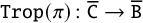


Remark 3.19. To allow for greater flexibility, we allow the total space
 $\mathcal C$
(but not
$\mathcal C$
(but not
 $\mathcal B$
, for simplicity of the exposition) to have self-intersections, that is to be a toroidal embedding without self-intersections only étale locally. There still is an associated cone complex
$\mathcal B$
, for simplicity of the exposition) to have self-intersections, that is to be a toroidal embedding without self-intersections only étale locally. There still is an associated cone complex
 ${{ \mathtt C}}$
, albeit one in which some cones have some of their faces glued together. One can remove the self-intersections by blowing up
${{ \mathtt C}}$
, albeit one in which some cones have some of their faces glued together. One can remove the self-intersections by blowing up
 $\mathcal C$
according to a suitable subdivision of
$\mathcal C$
according to a suitable subdivision of
 ${{ \mathtt C}}$
(essentially, the only thing that can go wrong is the existence of loops in the fibers; these need to be subdivided), but this comes at the cost of trading a family of stable curves for one of semistable curves.
${{ \mathtt C}}$
(essentially, the only thing that can go wrong is the existence of loops in the fibers; these need to be subdivided), but this comes at the cost of trading a family of stable curves for one of semistable curves.
Example 3.20. While the strata
 $O(\sigma )$
and their closures
$O(\sigma )$
and their closures
 $V(\sigma )$
are always irreducible, condition (3) in Definition 3.18 is not superfluous. It can happen that the fibers of
$V(\sigma )$
are always irreducible, condition (3) in Definition 3.18 is not superfluous. It can happen that the fibers of
 $V(\sigma )\to \pi (V(\sigma ))$
are reducible, but because of the monodromy action on the irreducible components, the domain
$V(\sigma )\to \pi (V(\sigma ))$
are reducible, but because of the monodromy action on the irreducible components, the domain
 $V(\sigma )$
is still irreducible. As an example consider the family of plane curves over
$V(\sigma )$
is still irreducible. As an example consider the family of plane curves over ![]() given by a union of three lines as
given by a union of three lines as
 $$ \begin{align} &\hspace{-50pt} \{(t-1)x+(t-\zeta)y+ (t-\zeta^2)z=0\} \quad\cup \nonumber \\ &\qquad \cup \quad\{(t-\zeta)x+(t-\zeta^2)y+ (t-1)z=0\} \quad \cup \nonumber \\ &\hspace{100pt} \quad \cup \quad \{(t-\zeta^2)x+(t-1)y+ (t-\zeta)z=0\} , \end{align} $$
where ![]() denotes a primitive third root of unity. Traveling from
denotes a primitive third root of unity. Traveling from
 $t=1$
to
$t=1$
to
 $t=\zeta $
permutes the three lines cyclically, and in particular the family descends to an irreducible family over
$t=\zeta $
permutes the three lines cyclically, and in particular the family descends to an irreducible family over ![]() whose fibers are unions of three lines in a plane that do not meet in a point. The construction of this example already shows how to fix families in which condition (3) is violated: one has to pass to an étale cover that trivializes the monodromy action on the components of the fibers.
whose fibers are unions of three lines in a plane that do not meet in a point. The construction of this example already shows how to fix families in which condition (3) is violated: one has to pass to an étale cover that trivializes the monodromy action on the components of the fibers.
Proposition 3.21. Let
 $\pi :\mathcal {C} \to \mathcal {B}$
be a tropicalizable family of stable, n-marked logarithmic curves, and let
$\pi :\mathcal {C} \to \mathcal {B}$
be a tropicalizable family of stable, n-marked logarithmic curves, and let
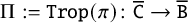 ${\Pi }:={\mathtt {Trop}}(\pi )\colon \overline {{ \mathtt C}}\to \overline {{ \mathtt B}}$
be its tropicalization. Then the maps f and
${\Pi }:={\mathtt {Trop}}(\pi )\colon \overline {{ \mathtt C}}\to \overline {{ \mathtt B}}$
be its tropicalization. Then the maps f and
 $f_\star $
from diagram (3.33) are linear.
$f_\star $
from diagram (3.33) are linear.
Proof. We first show the linearity of f on the interior
 ${ \mathtt B}$
of
${ \mathtt B}$
of
 $\overline { \mathtt B}$
. Let
$\overline { \mathtt B}$
. Let
 $b_0\in { \mathtt B}$
and let
$b_0\in { \mathtt B}$
and let
 $\sigma $
be the unique cone of
$\sigma $
be the unique cone of
 ${ \mathtt B}$
with
${ \mathtt B}$
with
 $b_0\in \sigma ^\diamond $
. Let G be the cycle-rigidified, n-marked, genus-g stable graph such that
$b_0\in \sigma ^\diamond $
. Let G be the cycle-rigidified, n-marked, genus-g stable graph such that
 $f(b_0) \in \sigma _G^\diamond $
. As the combinatorial type of the fibers of
$f(b_0) \in \sigma _G^\diamond $
. As the combinatorial type of the fibers of
 ${\Pi }$
remains constant on
${\Pi }$
remains constant on
 $\sigma ^\diamond $
, we have
$\sigma ^\diamond $
, we have
 $f(\sigma ^\diamond )\subseteq \sigma _G^\diamond $
and f and
$f(\sigma ^\diamond )\subseteq \sigma _G^\diamond $
and f and
 $f_\star $
induce an identification of the combinatorial type of
$f_\star $
induce an identification of the combinatorial type of
 $\overline { \mathtt C}_b$
with G for every
$\overline { \mathtt C}_b$
with G for every
 $b\in \sigma ^\diamond $
. Since linear functions on
$b\in \sigma ^\diamond $
. Since linear functions on
 ${\overline {\mathcal V}_{g,n}}$
are generated by vertex and edge primitive cross ratios ([Reference Cavalieri, Gross and Markwig6, Proposition 4.13]), we show linearity of f by showing that the pullback of a primitive cross ratio is linear on
${\overline {\mathcal V}_{g,n}}$
are generated by vertex and edge primitive cross ratios ([Reference Cavalieri, Gross and Markwig6, Proposition 4.13]), we show linearity of f by showing that the pullback of a primitive cross ratio is linear on
 ${ \mathtt B}$
.
${ \mathtt B}$
.
Let
 $c=c_{((f_s,f_e),(f_{-1},f_1))}$
be a primitive cross ratio of vertex type at a rational vertex v of G with associated function
$c=c_{((f_s,f_e),(f_{-1},f_1))}$
be a primitive cross ratio of vertex type at a rational vertex v of G with associated function
 $\xi _c$
on
$\xi _c$
on
 $({\overline {\mathcal V}_{g,n}})^{\sigma _G}$
. We show that
$({\overline {\mathcal V}_{g,n}})^{\sigma _G}$
. We show that
 $f^*\xi _c$
is linear on
$f^*\xi _c$
is linear on
 $\mathtt B^\sigma $
.
$\mathtt B^\sigma $
.
We may assume, possibly after subdividing some cones of
 ${ \mathtt B}$
, that
${ \mathtt B}$
, that
 ${ \mathtt B}^\sigma $
is simply connected. We may also assume, possibly after subdividing some cones of
${ \mathtt B}^\sigma $
is simply connected. We may also assume, possibly after subdividing some cones of
 $\overline { \mathtt C}$
, that the four flags
$\overline { \mathtt C}$
, that the four flags
 $f_s, f_e, f_{-1}, f_1$
belong to distinct edges in each fiber. Then the vertex v defines a component
$f_s, f_e, f_{-1}, f_1$
belong to distinct edges in each fiber. Then the vertex v defines a component
 $V(v)$
of
$V(v)$
of
 $\mathcal C_{V(\sigma )}$
. The four tangent directions
$\mathcal C_{V(\sigma )}$
. The four tangent directions
 $f_s$
,
$f_s$
,
 $f_e$
,
$f_e$
,
 $f_{-1}$
, and
$f_{-1}$
, and
 $f_1$
determine four sections of
$f_1$
determine four sections of
 $V(v)$
and thus a morphism
$V(v)$
and thus a morphism
 $$ \begin{align} V(\sigma)\to \overline{\mathcal M}_{0,4}; \end{align} $$
precomposing its tropicalization with the map quotienting
 $\sigma $
, we obtain
$\sigma $
, we obtain
 ${ \mathtt B}^\sigma \to \mathcal M_{0,4}^{\mathtt {trop}}$
. Since
${ \mathtt B}^\sigma \to \mathcal M_{0,4}^{\mathtt {trop}}$
. Since
 $f^*\xi _c$
agrees with the pullback of the appropriate cross ratio from
$f^*\xi _c$
agrees with the pullback of the appropriate cross ratio from
 $\mathcal M_{0,4}^{\mathtt {trop}}$
, linearity follows from Theorem 3.17.
$\mathcal M_{0,4}^{\mathtt {trop}}$
, linearity follows from Theorem 3.17.
Now let
 $c=c_{(e, (f_s,f_e), (f_{-1},f_1))}$
be a primitive cross ratio of edge type on G at an edge e. First assume that there exists a face
$c=c_{(e, (f_s,f_e), (f_{-1},f_1))}$
be a primitive cross ratio of edge type on G at an edge e. First assume that there exists a face
 $\tau $
of
$\tau $
of
 $\sigma $
such that
$\sigma $
such that
 $f(\tau ^\diamond )\subseteq \sigma _{\overline G}$
for some edge contraction
$f(\tau ^\diamond )\subseteq \sigma _{\overline G}$
for some edge contraction
 $\overline G$
of G in which e got contracted to a genus-
$\overline G$
of G in which e got contracted to a genus-
 $0$
vertex v. Then
$0$
vertex v. Then
 $f_s$
,
$f_s$
,
 $f_e$
,
$f_e$
,
 $f_{-1}$
, and
$f_{-1}$
, and
 $f_1$
induce flags at v and in particular a primitive cross ratio
$f_1$
induce flags at v and in particular a primitive cross ratio
 $\overline c=c_{((f_s,f_e),(f_1,f_1))}$
of vertex type on
$\overline c=c_{((f_s,f_e),(f_1,f_1))}$
of vertex type on
 $\overline G$
. By the vertex type case above, the function
$\overline G$
. By the vertex type case above, the function
 $f^*\xi _{\overline c}$
is linear on
$f^*\xi _{\overline c}$
is linear on
 $\mathtt B^\tau $
, and by Lemma 3.2 the restriction
$\mathtt B^\tau $
, and by Lemma 3.2 the restriction
 $f^*\xi _{\overline c}\vert _{\mathtt {B}^\sigma }$
is linear on
$f^*\xi _{\overline c}\vert _{\mathtt {B}^\sigma }$
is linear on
 $\mathtt B^\sigma $
. But
$\mathtt B^\sigma $
. But
 $f^*\xi _{\overline c}\vert _{\mathtt B^\sigma }$
coincides with
$f^*\xi _{\overline c}\vert _{\mathtt B^\sigma }$
coincides with
 $f^*\xi _c$
on
$f^*\xi _c$
on
 $\mathtt B^\sigma $
, concluding the proof in this case.
$\mathtt B^\sigma $
, concluding the proof in this case.
Next, assume that for any face of
 $\sigma $
where the edge e gets contracted, a vertex of positive genus is formed. We can view
$\sigma $
where the edge e gets contracted, a vertex of positive genus is formed. We can view
 $\mathcal C$
as the base of a family of
$\mathcal C$
as the base of a family of
 $(n\sqcup \{\star \})$
-marked stable curves
$(n\sqcup \{\star \})$
-marked stable curves
 $$ \begin{align} \pi_\star\colon \mathcal C_\star\to \mathcal C. \end{align} $$
The cycle rigidification of
 ${\Pi }$
induced by the maps f and
${\Pi }$
induced by the maps f and
 $f_\star $
from diagram (3.33) produces a cycle rigidification of the family
$f_\star $
from diagram (3.33) produces a cycle rigidification of the family
that is a Cartesian TPL-diagram

Let
 $\sigma _e\in \Sigma $
be the cone over
$\sigma _e\in \Sigma $
be the cone over
 $\sigma $
whose fibers corresponds to e. The stratum
$\sigma $
whose fibers corresponds to e. The stratum
 $V(\sigma _e)$
is the node corresponding to e in every fiber of
$V(\sigma _e)$
is the node corresponding to e in every fiber of
 $\mathcal C_{V(\sigma )}\to V(\sigma )$
and thus the restriction of
$\mathcal C_{V(\sigma )}\to V(\sigma )$
and thus the restriction of
 $\pi $
defines an isomorphism
$\pi $
defines an isomorphism
 $V(\sigma _e)\to V(\sigma )$
. The pull-back
$V(\sigma _e)\to V(\sigma )$
. The pull-back
 $\mu _\star ^*\xi _c$
is a cross ratio on
$\mu _\star ^*\xi _c$
is a cross ratio on
 ${\overline {\mathcal V}_{g,n\sqcup \{\star \}}}$
, although not a primitive one. More precisely, if
${\overline {\mathcal V}_{g,n\sqcup \{\star \}}}$
, although not a primitive one. More precisely, if
 $G_\star $
denotes the rigidified
$G_\star $
denotes the rigidified
 $(n\sqcup \{\star \})$
-marked graph, obtained by introducing a vertex v on e in G and attaching a
$(n\sqcup \{\star \})$
-marked graph, obtained by introducing a vertex v on e in G and attaching a
 $\star -$
marked leg
$\star -$
marked leg
 $l_\star $
at v, then
$l_\star $
at v, then
 $f_\star (\sigma _e)\subseteq \sigma _{G_\star }$
and c induces a cross ratio datum on
$f_\star (\sigma _e)\subseteq \sigma _{G_\star }$
and c induces a cross ratio datum on
 $G_\star $
by ignoring the fact that e has been subdivided. If
$G_\star $
by ignoring the fact that e has been subdivided. If
 $e_1$
and
$e_1$
and
 $e_2$
denote the two edges adjacent to v in the order seen when traversing e according to c, and
$e_2$
denote the two edges adjacent to v in the order seen when traversing e according to c, and
 $g_1$
and
$g_1$
and
 $g_2$
are the corresponding half-edges starting at v, as shown in Figure 5, then we have
$g_2$
are the corresponding half-edges starting at v, as shown in Figure 5, then we have
 $$ \begin{align} \mu_\star^*\xi_c = \xi_{(e_1,(f_s,l_\star),(f_{-1},g_2))}+ \xi_{(e_2,(l_\star,f_e),(g_2,f_1))} \end{align} $$
The two edges
 $e_1$
and
$e_1$
and
 $e_2$
are contracted on the two faces of
$e_2$
are contracted on the two faces of
 $\sigma _e$
that map isomorphically onto
$\sigma _e$
that map isomorphically onto
 $\sigma $
and correspond to the two vertices of e. Therefore, for each of the two primitive cross ratio summands in (3.39) we are in the special situation from before: the edge of the edge-type primitive cross ratio is contracted to a genus zero vertex. Algebraically, this yields
$\sigma $
and correspond to the two vertices of e. Therefore, for each of the two primitive cross ratio summands in (3.39) we are in the special situation from before: the edge of the edge-type primitive cross ratio is contracted to a genus zero vertex. Algebraically, this yields
 $$ \begin{align} \mathcal O_{V(\sigma_e)}&\cong \left(\mathcal O_{\mathcal C_{\sigma_e}}(f_\star^*\xi_{(e_1,(f_s,l_\star),(f_{-1},g_2))})\otimes \mathcal O_{\mathcal C_{\sigma_e}}(f_\star^*\xi_{(e_2,(l_\star,f_e),(g_2,f_1))})\right)\vert_{V(\sigma_e)} \cong \nonumber \\ &\quad \cong \mathcal O_{\mathcal C_{\sigma_e}}(f_\star^*\mu_\star^*\xi_c)\vert_{V(\sigma_e)}\cong \mathcal O_{\mathcal C_{\sigma_e}}({\Pi }^*f^* \xi_c\vert_{\sigma_e})\vert_{V(\sigma_e)}\cong \left(\pi^*\mathcal O_{\mathcal B_{\sigma}}(f^*\xi_c)\right)\Big\vert_{V(\sigma_e)} . \end{align} $$
As we have noticed before,
 $\pi $
induces an isomorphism
$\pi $
induces an isomorphism
 $V(\sigma _e)\to V(\sigma )$
, so we conclude that
$V(\sigma _e)\to V(\sigma )$
, so we conclude that
 $$ \begin{align} \mathcal O_{\mathcal B_{\sigma}}(f^*\xi_c)\vert_{V(\sigma)}\cong \mathcal O_{V(\sigma)} , \end{align} $$
which is equivalent to
 $f^\ast \xi _c$
being linear on
$f^\ast \xi _c$
being linear on
 $\mathtt B^\sigma $
.
$\mathtt B^\sigma $
.
The subdivision of the edge e in
 $G_\star $
.
$G_\star $
.

To show that f is also linear on the boundary of
 $\mathtt B$
it suffices to note that on both source (by Definition 3.10) and target (by [Reference Cavalieri, Gross and Markwig6, Lemma 4.16]), the affine structure near the boundary is induced by the affine structure on the interior in the sense that the affine functions at the boundary are precisely the continuous extensions of affine functions on the interior.
$\mathtt B$
it suffices to note that on both source (by Definition 3.10) and target (by [Reference Cavalieri, Gross and Markwig6, Lemma 4.16]), the affine structure near the boundary is induced by the affine structure on the interior in the sense that the affine functions at the boundary are precisely the continuous extensions of affine functions on the interior.
To show that
 $f_\star $
is linear one applies the same arguments to the map
$f_\star $
is linear one applies the same arguments to the map
 $\pi _\star $
and the rigidification displayed in (3.38).
$\pi _\star $
and the rigidification displayed in (3.38).
Proposition 3.22. With the set-up and notation of Proposition 3.21, let
 $x\in {\overline { \mathtt C}}$
. If x has genus
$x\in {\overline { \mathtt C}}$
. If x has genus
 $0$
, then all functions in
$0$
, then all functions in
 $\operatorname {\mathrm {Aff}}_{{{ \mathtt C}},x}$
are linear on the fibers of
$\operatorname {\mathrm {Aff}}_{{{ \mathtt C}},x}$
are linear on the fibers of
 ${\Pi }$
close to x. Moreover, we have an exact sequence
${\Pi }$
close to x. Moreover, we have an exact sequence
 $$ \begin{align} 0 \to \operatorname{\mathrm{Aff}}_{\overline{ \mathtt B},{\Pi }(x)}\to \operatorname{\mathrm{Aff}}_{{\overline{ \mathtt C}},x} \to \Omega^1_{{{\overline{ \mathtt C}}}_{{\Pi }(x)},x}\to 0 . \end{align} $$
If x is a vertex (of genus
 $0$
) in its fiber, or is on an edge adjacent to a vertex of genus
$0$
) in its fiber, or is on an edge adjacent to a vertex of genus
 $0$
, then
$0$
, then
 $\Omega ^1_{{{\overline { \mathtt C}}}_{{\Pi }(x)},x}$
consists of the differentials of all harmonic functions.
$\Omega ^1_{{{\overline { \mathtt C}}}_{{\Pi }(x)},x}$
consists of the differentials of all harmonic functions.
Proof. The injectivity of the pull-back is obvious, so is the surjectivity of restriction to the fiber (we consider the fiber with the induced affine structure). We show the harmonicity of affine functions on fibers and the exactness in the middle simultaneously.
We first prove the proposition in the case when
 $x\in {{{ \mathtt C}}}$
. Suppose x is on an edge in its fiber. In that case a function
$x\in {{{ \mathtt C}}}$
. Suppose x is on an edge in its fiber. In that case a function
 $\phi \in \operatorname {\mathrm {Aff}}_{{{{ \mathtt C}}},x}$
is linear, and hence harmonic, on all fibers in a neighborhood of x. If
$\phi \in \operatorname {\mathrm {Aff}}_{{{{ \mathtt C}}},x}$
is linear, and hence harmonic, on all fibers in a neighborhood of x. If
 $\phi \vert _{{\Pi }^{-1}\{{\Pi }(x)\}}$
is constant near x, then
$\phi \vert _{{\Pi }^{-1}\{{\Pi }(x)\}}$
is constant near x, then
 $\phi $
is constant on fibers on a small neighborhood of x. Let
$\phi $
is constant on fibers on a small neighborhood of x. Let
 $\sigma \in {{{ \mathtt C}}}$
be the unique cone with
$\sigma \in {{{ \mathtt C}}}$
be the unique cone with
 $x\in \sigma ^\diamond $
and let
$x\in \sigma ^\diamond $
and let
 $\tau ={\Pi }({{\sigma }})$
. By definition of the affine structure on
$\tau ={\Pi }({{\sigma }})$
. By definition of the affine structure on
 ${{{ \mathtt C}}}$
,
${{{ \mathtt C}}}$
,
 $\phi $
defines a piecewise linear function on
$\phi $
defines a piecewise linear function on
 ${{{ \mathtt C}}}^\sigma $
, and
${{{ \mathtt C}}}^\sigma $
, and
 $\phi $
is constant on all the fibers of the induced map
$\phi $
is constant on all the fibers of the induced map
 ${{{ \mathtt C}}}^\sigma \to { \mathtt B}^\tau $
. Taking any section
${{{ \mathtt C}}}^\sigma \to { \mathtt B}^\tau $
. Taking any section
 ${ \mathtt B}^\tau \to {{{ \mathtt C}}}^\sigma $
of this map (for example a section corresponding to one of the two vertices of the edge on which x sits), we obtain a piecewise linear function
${ \mathtt B}^\tau \to {{{ \mathtt C}}}^\sigma $
of this map (for example a section corresponding to one of the two vertices of the edge on which x sits), we obtain a piecewise linear function
 $\chi $
on
$\chi $
on
 ${ \mathtt B}^\tau $
with
${ \mathtt B}^\tau $
with
 ${\Pi }^*\chi =\phi $
. The stratum
${\Pi }^*\chi =\phi $
. The stratum
 $V(\sigma )$
is a node in each fiber, and the projection
$V(\sigma )$
is a node in each fiber, and the projection
 $\pi \vert _{V(\sigma )} \colon V(\sigma )\to V(\tau )$
is an isomorphism. We have
$\pi \vert _{V(\sigma )} \colon V(\sigma )\to V(\tau )$
is an isomorphism. We have
 $$ \begin{align} \pi\vert_{V(\sigma)}^* \mathcal O_{\mathcal B_\tau}(\chi)\vert_{V(\tau)}\cong \mathcal O_{\mathcal C_\sigma}({\Pi }^*\chi)\vert_{V(\sigma)} \cong \mathcal O_{\mathcal C_\sigma}(\phi)\vert_{V(\sigma)} \cong \mathcal O_{V(\sigma)} , \end{align} $$
where the last isomorphism follows because
 $\phi $
is affine; we conclude that
$\phi $
is affine; we conclude that
 $\chi $
is affine on
$\chi $
is affine on
 ${ \mathtt B}$
.
${ \mathtt B}$
.
Now suppose x is a vertex of genus
 $0$
, let
$0$
, let
 $\sigma $
and
$\sigma $
and
 $\tau $
be as above, and let
$\tau $
be as above, and let
 $\phi \in \operatorname {\mathrm {Aff}}_{{ \mathtt C},x}$
. Let e be an edge in the fiber of x that is adjacent to x. After subtracting a suitable cross ratio, which is harmonic on fibers and affine by Proposition 3.21, we may assume that
$\phi \in \operatorname {\mathrm {Aff}}_{{ \mathtt C},x}$
. Let e be an edge in the fiber of x that is adjacent to x. After subtracting a suitable cross ratio, which is harmonic on fibers and affine by Proposition 3.21, we may assume that
 $\phi $
is constant on e. So by the case where x was on an edge, there exists an affine function
$\phi $
is constant on e. So by the case where x was on an edge, there exists an affine function
 $\chi \in \operatorname {\mathrm {Aff}}_{{ \mathtt B},{\Pi }(x)}$
such that
$\chi \in \operatorname {\mathrm {Aff}}_{{ \mathtt B},{\Pi }(x)}$
such that
 $\phi -{\Pi }^*\chi $
vanishes on e. In particular, by replacing
$\phi -{\Pi }^*\chi $
vanishes on e. In particular, by replacing
 $\phi $
with this difference of affine functions, we may assume that
$\phi $
with this difference of affine functions, we may assume that
 $\phi \vert _{\sigma }=0$
. By Proposition 3.12,
$\phi \vert _{\sigma }=0$
. By Proposition 3.12,
 $\phi $
is induced by an affine function
$\phi $
is induced by an affine function
 $\overline \phi $
on
$\overline \phi $
on
 ${{{ \mathtt C}}}^\sigma /\sigma ={{{ \mathtt C}}}_{V(\sigma )}$
. Let
${{{ \mathtt C}}}^\sigma /\sigma ={{{ \mathtt C}}}_{V(\sigma )}$
. Let
 $T_x({{{ \mathtt C}}}_{{\Pi }(x)})$
denote the set of half-edges starting at x in its fiber. For each
$T_x({{{ \mathtt C}}}_{{\Pi }(x)})$
denote the set of half-edges starting at x in its fiber. For each
 $h\in T_x({{{ \mathtt C}}}_{{\Pi }(x)})$
let
$h\in T_x({{{ \mathtt C}}}_{{\Pi }(x)})$
let
 $m_h$
be the slope of
$m_h$
be the slope of
 $\phi $
in the direction of h, and let
$\phi $
in the direction of h, and let
 $\sigma _h$
be the cone of
$\sigma _h$
be the cone of
 ${{{ \mathtt C}}}$
spanned by
${{{ \mathtt C}}}$
spanned by
 $\sigma $
and h. Then the normalization
$\sigma $
and h. Then the normalization
 $\widetilde V(\sigma )$
of the stratum
$\widetilde V(\sigma )$
of the stratum
 $V(\sigma )$
is a family of
$V(\sigma )$
is a family of
 $T_x({{{ \mathtt C}}}_{{\Pi }(x)})$
-marked rational stable curves over
$T_x({{{ \mathtt C}}}_{{\Pi }(x)})$
-marked rational stable curves over
 $V(\tau )$
, and
$V(\tau )$
, and
 $V(\sigma _h)$
is the section of this family corresponding to
$V(\sigma _h)$
is the section of this family corresponding to
 $h\in T_x({{{ \mathtt C}}}_{{\Pi }(x)})$
. The fact that
$h\in T_x({{{ \mathtt C}}}_{{\Pi }(x)})$
. The fact that
 $\phi $
is affine means that the divisor
$\phi $
is affine means that the divisor
 $$ \begin{align} \sum_{h\in T_x({{{ \mathtt C}}}_{{\Pi }(x)})} m_h V(\sigma_h) \end{align} $$
is rationally equivalent to
 $0$
on
$0$
on
 $\widetilde V(\sigma )$
. Since the fiber of
$\widetilde V(\sigma )$
. Since the fiber of
 $\widetilde V(\sigma )\to V(\tau )$
over any
$\widetilde V(\sigma )\to V(\tau )$
over any
 $y\in O(\tau )$
is isomorphic to
$y\in O(\tau )$
is isomorphic to ![]() , we conclude that
, we conclude that
 $\sum _h m_h=0$
, because every divisor on
$\sum _h m_h=0$
, because every divisor on ![]() rationally equivalent to
rationally equivalent to
 $0$
has degree
$0$
has degree
 $0$
. This shows that
$0$
. This shows that
 $\phi $
is harmonic at x. Onto exactness in the middle of (3.43), if x is a vertex and
$\phi $
is harmonic at x. Onto exactness in the middle of (3.43), if x is a vertex and
 $\phi \vert _{{\Pi }^{-1}\{{\Pi }(x)\}}$
is constant near x, then it is constant on an edge adjacent to x; by the case where x was on an edge we obtain an affine function
$\phi \vert _{{\Pi }^{-1}\{{\Pi }(x)\}}$
is constant near x, then it is constant on an edge adjacent to x; by the case where x was on an edge we obtain an affine function
 $\chi \in \operatorname {\mathrm {Aff}}_{{ \mathtt B},{\Pi }(x)}$
with
$\chi \in \operatorname {\mathrm {Aff}}_{{ \mathtt B},{\Pi }(x)}$
with
 $\phi ={\Pi }^*\chi $
.
$\phi ={\Pi }^*\chi $
.
Let x be either a rational vertex or adjacent to a genus
 $0$
vertex in its fiber. By the linearity of
$0$
vertex in its fiber. By the linearity of
 $f_\star $
(Proposition 3.21), all (pull-backs of) cross ratios are linear on
$f_\star $
(Proposition 3.21), all (pull-backs of) cross ratios are linear on
 ${{{ \mathtt C}}}$
. By the condition on x, by [Reference Cavalieri, Gross and Markwig6, Proposition 4.24] there are enough cross ratio functions defined at x to realize all possible differentials of harmonic functions on the fiber.
${{{ \mathtt C}}}$
. By the condition on x, by [Reference Cavalieri, Gross and Markwig6, Proposition 4.24] there are enough cross ratio functions defined at x to realize all possible differentials of harmonic functions on the fiber.
It remains to analyze the case where
 $x\in \overline { \mathtt C}\setminus { \mathtt C}$
. Let
$x\in \overline { \mathtt C}\setminus { \mathtt C}$
. Let
 $\delta $
be the unique cone of
$\delta $
be the unique cone of
 ${ \mathtt C}$
with
${ \mathtt C}$
with
 $x\in { \mathtt C}^\delta /\delta $
and let
$x\in { \mathtt C}^\delta /\delta $
and let
 $\theta ={\Pi }(\delta )$
, which is a cone in
$\theta ={\Pi }(\delta )$
, which is a cone in
 ${ \mathtt B}$
. We can either have
${ \mathtt B}$
. We can either have
 $\dim (\delta )=\dim (\theta )+1$
or
$\dim (\delta )=\dim (\theta )+1$
or
 $\dim (\delta )=\dim (\theta )$
. In the first case, the point x is either the endpoint of a leg or a node at infinity in its fiber (see [Reference Cavalieri, Gross and Markwig6, p. 14]). It follows that
$\dim (\delta )=\dim (\theta )$
. In the first case, the point x is either the endpoint of a leg or a node at infinity in its fiber (see [Reference Cavalieri, Gross and Markwig6, p. 14]). It follows that
 $\Omega ^1_{{\Pi }(x),x}=0$
and we need to show that the pull-back
$\Omega ^1_{{\Pi }(x),x}=0$
and we need to show that the pull-back
 $\operatorname {\mathrm {Aff}}_{\overline { \mathtt B},\Pi (X)}\to \operatorname {\mathrm {Aff}}_{\overline { \mathtt C},x}$
is an isomorphism. The morphism
$\operatorname {\mathrm {Aff}}_{\overline { \mathtt B},\Pi (X)}\to \operatorname {\mathrm {Aff}}_{\overline { \mathtt C},x}$
is an isomorphism. The morphism
 $V(\delta )\to V(\theta )$
induced by
$V(\delta )\to V(\theta )$
induced by
 $\pi $
is an isomorphism because
$\pi $
is an isomorphism because
 $V(\delta )$
either consists of a single marked point or a single node in each fiber over
$V(\delta )$
either consists of a single marked point or a single node in each fiber over
 $V(\theta )$
. So
$V(\theta )$
. So
 $\pi $
also induces an isomorphism
$\pi $
also induces an isomorphism
 $\Sigma _{V(\delta )}\to \Sigma _{V(\theta )}$
of tropical spaces and we are done by Proposition 3.12. In the second case, that is, when
$\Sigma _{V(\delta )}\to \Sigma _{V(\theta )}$
of tropical spaces and we are done by Proposition 3.12. In the second case, that is, when
 $\delta $
and
$\delta $
and
 $\theta $
have the same dimension, a neighborhood of x in
$\theta $
have the same dimension, a neighborhood of x in
 $\overline { \mathtt C}_{\Pi (x)}$
is contained in
$\overline { \mathtt C}_{\Pi (x)}$
is contained in
 ${ \mathtt C}^\delta /\delta $
. It therefore suffices to prove the assertion for the family
${ \mathtt C}^\delta /\delta $
. It therefore suffices to prove the assertion for the family
 $$\begin{align*}\Sigma_{V(\delta)}\cong { \mathtt C}^\delta/\delta\to { \mathtt B}^\theta/\theta\cong \Sigma_{V(\theta)} , \end{align*}$$
where the canonical isomorphisms come from Proposition 3.12. This family is the tropicalization of the induced family of curves
 $V(\delta )\to V(\theta )$
and x is in the interior of
$V(\delta )\to V(\theta )$
and x is in the interior of
 $\Sigma _{V(\delta )}$
, so we have reduced to the case that we already proved.
$\Sigma _{V(\delta )}$
, so we have reduced to the case that we already proved.
Remark 3.23. Consider the set
 ${ \mathtt U}\subseteq {{{ \mathtt C}}}$
of all genus-
${ \mathtt U}\subseteq {{{ \mathtt C}}}$
of all genus-
 $0$
points that are either vertices or on an edge adjacent to a genus-
$0$
points that are either vertices or on an edge adjacent to a genus-
 $0$
vertex. The locus
$0$
vertex. The locus
 ${ \mathtt U}$
is closely related to the locus
${ \mathtt U}$
is closely related to the locus
 $\mathcal V^{\mathrm {good}}_{g,n}$
introduced in [Reference Cavalieri, Gross and Markwig6, Definition 4.22]. More precisely, we have
$\mathcal V^{\mathrm {good}}_{g,n}$
introduced in [Reference Cavalieri, Gross and Markwig6, Definition 4.22]. More precisely, we have
 $$ \begin{align} f^{-1}\mathcal V^{\mathrm{good}}_{g,n}= \{y \mid {{{ \mathtt C}}}_y\subseteq { \mathtt U}\} \, \end{align} $$
where
 ${{{ \mathtt C}}}_y$
denotes the fiber over y. One can view
${{{ \mathtt C}}}_y$
denotes the fiber over y. One can view
 ${ \mathtt U}$
as the locus where
${ \mathtt U}$
as the locus where
 ${{{ \mathtt C}}}\to { \mathtt B}$
is a family of tropical curves in the sense of [Reference Cavalieri, Gross and Markwig6]. The affine structure on
${{{ \mathtt C}}}\to { \mathtt B}$
is a family of tropical curves in the sense of [Reference Cavalieri, Gross and Markwig6]. The affine structure on
 ${ \mathtt U}$
is completely determined by that on
${ \mathtt U}$
is completely determined by that on
 ${ \mathtt B}$
. Equivalently, the inclusion
${ \mathtt B}$
. Equivalently, the inclusion
 $$ \begin{align} { \mathtt U}\to { \mathtt B}\times_{{\overline {\mathcal V}_{g,n}}}{\overline {\mathcal V}_{g,n\sqcup \{\star\}}} , \end{align} $$
where the fiber product is taken in the category of tropical spaces, is an open immersion.
4 Tropicalizations of line bundles
Let X be a toroidal variety and let
 $\pi \colon L \to X$
be a line bundle on X. We equip the total space of L with the toroidal structure whose boundary is
$\pi \colon L \to X$
be a line bundle on X. We equip the total space of L with the toroidal structure whose boundary is
 $Z\cup \pi ^{-1}\partial X$
, where Z denotes the zero-section of the bundle. The cone complex
$Z\cup \pi ^{-1}\partial X$
, where Z denotes the zero-section of the bundle. The cone complex
 $\Sigma _L$
is naturally identified with
$\Sigma _L$
is naturally identified with
 $\Sigma _X\times \rho _Z$
, where
$\Sigma _X\times \rho _Z$
, where
 $\rho _Z$
is the ray of
$\rho _Z$
is the ray of
 $\Sigma _L$
corresponding to the boundary divisor Z. Via the construction from Section 3, we obtain an affine structure on
$\Sigma _L$
corresponding to the boundary divisor Z. Via the construction from Section 3, we obtain an affine structure on
 $\overline \Sigma _X\times \overline \rho _Z$
.
$\overline \Sigma _X\times \overline \rho _Z$
.
Definition 4.1. Extend the affine structure on
 $\overline \Sigma _X\times (\overline \rho _Z\setminus \{0\})$
to
$\overline \Sigma _X\times (\overline \rho _Z\setminus \{0\})$
to ![]() by linearity, where we identify
by linearity, where we identify ![]() with
with
 $\overline {\rho }_Z\setminus \{0\}$
. We call the morphism
$\overline {\rho }_Z\setminus \{0\}$
. We call the morphism
of spaces with affine structures the tropicalization of L and denote it by
 ${\mathtt {Trop}}(L)$
.
${\mathtt {Trop}}(L)$
.
Remark 4.2. We describe an equivalent way of defining
 ${\mathtt {Trop}}(L)$
: first compactify the total space L by adding a section at infinity, that is consider the projective bundle
${\mathtt {Trop}}(L)$
: first compactify the total space L by adding a section at infinity, that is consider the projective bundle ![]() ; the boundary consists of the union of the pull-back of
; the boundary consists of the union of the pull-back of
 $\partial X$
with the two sections. If
$\partial X$
with the two sections. If
 $\rho _\infty $
is the ray of
$\rho _\infty $
is the ray of
 $\Sigma _{P_L}$
corresponding to the section at infinity, then
$\Sigma _{P_L}$
corresponding to the section at infinity, then
 ${\mathtt {Trop}}(L)$
is the complement of
${\mathtt {Trop}}(L)$
is the complement of
 $\Sigma _{P_L}^{\rho _\infty }/\rho _\infty $
in
$\Sigma _{P_L}^{\rho _\infty }/\rho _\infty $
in
 $\overline \Sigma _{P_L}$
. More concisely, we add a section at infinity, tropicalize, and then remove the tropical section at infinity.
$\overline \Sigma _{P_L}$
. More concisely, we add a section at infinity, tropicalize, and then remove the tropical section at infinity.
The tropicalization of L is not necessarily a tropical line bundle (see §2.4), as we illustrate in the following example.
Example 4.3. We present here three examples of tropicalization of a line bundle
 $\pi \colon L\to X$
on a toroidal variety X with exactly one boundary divisor H. The extended tropicalization
$\pi \colon L\to X$
on a toroidal variety X with exactly one boundary divisor H. The extended tropicalization
 $\overline {\Sigma }_X$
of X is the closed segment
$\overline {\Sigma }_X$
of X is the closed segment
 $[0, \infty ]$
and we denote by
$[0, \infty ]$
and we denote by
 $\{V_0, V_\infty \}$
the open cover
$\{V_0, V_\infty \}$
the open cover
 $\{[0, \infty ), (0, \infty ]\}$
. The map of extended cone complexes giving the tropicalization of L is depicted in Figure 6; in all three cases the combinatorics of the tropicalization is the same, what differs is the affine structure on the total space
$\{[0, \infty ), (0, \infty ]\}$
. The map of extended cone complexes giving the tropicalization of L is depicted in Figure 6; in all three cases the combinatorics of the tropicalization is the same, what differs is the affine structure on the total space ![]() . We describe the affine structure by giving the affine functions on the six types of open sets
. We describe the affine structure by giving the affine functions on the six types of open sets
 $\mathtt U_{ij}$
shaded in Figure 6. In each case we will denote
$\mathtt U_{ij}$
shaded in Figure 6. In each case we will denote ![]() .
.
The tropicalization of a line bundle on a toroidal space with a unique boundary divisor H. As suggested by the orientation of the picture, we call x a linear coordinate for the ray
 $\rho _H$
and y the coordinate for the ray
$\rho _H$
and y the coordinate for the ray
 $\rho _Z$
dual to the zero section
$\rho _Z$
dual to the zero section
 $Z\cong X$
.
$Z\cong X$
.

Case 1: ![]() ,
, ![]() .
.
The local affine functions are the following:

-
(a) since the open set
${ \mathtt U}_{0 \infty }$
contains the cell at infinity
$\rho _Z/\rho _Z$
, any affine function must be constant in y. The local function
$\alpha x+r$
is affine if and only if . We have (4.2)it follows that
$\alpha =0$
;
-
(b) affine functions need to be constant in y. We want to see when
$\mathcal {O}_{L}(\alpha \widetilde H)\vert _{Z\cap \widetilde H}\cong \mathcal {O}_{Z\cap \widetilde H}$
, but
$Z\cap \widetilde H$
consists of a single point, and therefore any line bundle restricted to it must be trivial. There is no condition on
$\alpha $
; -
(c) the set
${ \mathtt U}_{\infty \infty }$
contains the point
$(\infty , \infty )$
and therefore affine functions must be constant in x and y and therefore constant. -
(d) we are looking for functions of the form
$\alpha x+\beta y+r$
such that (4.3)setting
$\alpha +m\beta = 0$
shows that affine functions have the form
$\beta (y-mx)+r$
;
-
(e) in this case we are again restricting a line bundle on the total space of L to the point
$Z\cap \widetilde H$
, therefore always obtaining a trivial bundle. There is no restriction on the integral slopes of affine functions. -
(f) affine functions must be constant in x. The function
$\beta y+r$
is affine if
$\mathcal {O}_{L}(\beta \widetilde H)\vert _{\widetilde H}$
is trivial. But since , any line bundle may be trivialized and the result follows.


We see that
 ${\mathtt {Trop}}(L)$
is a tropical line bundle on
${\mathtt {Trop}}(L)$
is a tropical line bundle on
 $\overline {\Sigma }_X$
with Cartier data
$\overline {\Sigma }_X$
with Cartier data
 $\{(V_0, -mx),(V_\infty ,0)\}.$
Case 2: ![]() ,
, ![]() .
.
The local affine functions are the following:

We don’t go through the computations in detail, since they are very similar to those in the first case. To highlight what the difference is, we just look at what is different in computing the affine sections for the open set
 ${ \mathtt U}_{x y}$
: we are now looking for functions of the form
${ \mathtt U}_{x y}$
: we are now looking for functions of the form
 $\alpha x+\beta y+r$
such that
$\alpha x+\beta y+r$
such that
 $\mathcal {O}_{L}(\alpha \widetilde H+\beta Z)\vert _{Z\cap \widetilde H}\cong \mathcal {O}_{Z\cap \widetilde H}$
. Notice that
$\mathcal {O}_{L}(\alpha \widetilde H+\beta Z)\vert _{Z\cap \widetilde H}\cong \mathcal {O}_{Z\cap \widetilde H}$
. Notice that
 $Z\cap \widetilde H$
is now a hyperplane in
$Z\cap \widetilde H$
is now a hyperplane in ![]() , and it is therefore isomorphic to
, and it is therefore isomorphic to ![]() . We have
. We have
there must be a nontrivial relation between
 $\alpha $
and
$\alpha $
and
 $\beta $
in order for the line bundle to trivialize, yielding the result from
$\beta $
in order for the line bundle to trivialize, yielding the result from
 $(e)$
. In this case
$(e)$
. In this case
 ${\mathtt {Trop}}(L)$
is a (trivial) tropical line bundle on the cone complex
${\mathtt {Trop}}(L)$
is a (trivial) tropical line bundle on the cone complex
 $\Sigma _X$
, but not on the extended space
$\Sigma _X$
, but not on the extended space
 $\overline {\Sigma }_X$
.
$\overline {\Sigma }_X$
.
Case 3: ![]() ,
, ![]() . In this case the local affine functions are:
. In this case the local affine functions are:

Again, the computations are similar to the first case, so we just show the most interesting example. We compute the local sections
 $ \operatorname {\mathrm {Aff}}_{{\mathtt {Trop}} (L)}({ \mathtt U}_{0 y})$
. These are functions of the form
$ \operatorname {\mathrm {Aff}}_{{\mathtt {Trop}} (L)}({ \mathtt U}_{0 y})$
. These are functions of the form
 $\alpha x+\beta y+r$
such that
$\alpha x+\beta y+r$
such that ![]() . In this case:
. In this case:
where
 $V= c_1(L)$
denotes the class of the vertical fiber in
$V= c_1(L)$
denotes the class of the vertical fiber in ![]() . For the bundle to be trivial we must have
. For the bundle to be trivial we must have
 $\alpha =\beta =0$
. We thus see that
$\alpha =\beta =0$
. We thus see that
 ${\mathtt {Trop}}(L)$
is not a tropical line bundle on
${\mathtt {Trop}}(L)$
is not a tropical line bundle on
 $\Sigma _X$
.
$\Sigma _X$
.
We investigate when the tropicalization of a line bundle is indeed a tropical line bundle. We will say that a line bundle is tropicalizable when this happens.
Proposition 4.4. Let L be a line bundle on X with associated invertible sheaf
 $\mathcal L$
and let
$\mathcal L$
and let
 ${ \mathtt U}\subseteq ~\overline {\Sigma }_X$
be an open subcomplex. Then
${ \mathtt U}\subseteq ~\overline {\Sigma }_X$
be an open subcomplex. Then
 ${\mathtt {Trop}}(L)$
is a tropical line bundle on
${\mathtt {Trop}}(L)$
is a tropical line bundle on
 ${ \mathtt U}$
if and only if for every cell
${ \mathtt U}$
if and only if for every cell
 $\sigma /\tau $
of
$\sigma /\tau $
of
 ${ \mathtt U}$
there exists a function
${ \mathtt U}$
there exists a function
 $\phi _{\sigma /\tau }\in {\mathrm {sPL}}(\overline \Sigma _X^{\sigma /\tau })$
(see page 17) with
$\phi _{\sigma /\tau }\in {\mathrm {sPL}}(\overline \Sigma _X^{\sigma /\tau })$
(see page 17) with
 $$ \begin{align} \left(\mathcal O_{X_{\sigma}}(\phi_{\sigma/\tau}) \otimes \mathcal L\right)\vert_{V(\sigma)} \cong \mathcal O_{V(\sigma)} . \end{align} $$
In that case,
 ${\mathtt {Trop}}(L)$
is the tropical line bundle associated to the tropical Cartier divisor
${\mathtt {Trop}}(L)$
is the tropical line bundle associated to the tropical Cartier divisor
 $(\overline {\Sigma }_X^{\sigma /\tau },\phi _{\sigma /\tau })_{\sigma /\tau \subseteq { \mathtt U}}$
.
$(\overline {\Sigma }_X^{\sigma /\tau },\phi _{\sigma /\tau })_{\sigma /\tau \subseteq { \mathtt U}}$
.
Proof. The total space
 ${\mathtt {Trop}}(L)$
is a tropical line bundle on
${\mathtt {Trop}}(L)$
is a tropical line bundle on
 ${ \mathtt U}$
if and only if for every cell
${ \mathtt U}$
if and only if for every cell
 $\sigma /\tau $
of
$\sigma /\tau $
of
 ${ \mathtt U}$
there exists exactly one element in
${ \mathtt U}$
there exists exactly one element in
 $\operatorname {\mathrm {Aff}}_{\Sigma _L}({\overline \Sigma _L}^{(\sigma /\tau )\times \rho _Z})/\operatorname {\mathrm {Aff}}_{ \overline \Sigma _X}( \overline \Sigma _X^{\sigma /\tau })$
with slope
$\operatorname {\mathrm {Aff}}_{\Sigma _L}({\overline \Sigma _L}^{(\sigma /\tau )\times \rho _Z})/\operatorname {\mathrm {Aff}}_{ \overline \Sigma _X}( \overline \Sigma _X^{\sigma /\tau })$
with slope
 $1$
along the ray
$1$
along the ray
 $\rho _Z$
dual to the zero section of L. Let I denote the set of functions in
$\rho _Z$
dual to the zero section of L. Let I denote the set of functions in
 ${\mathrm {sPL}}({\overline \Sigma _L}^{(\sigma /\tau )\times \rho _Z})$
with slope
${\mathrm {sPL}}({\overline \Sigma _L}^{(\sigma /\tau )\times \rho _Z})$
with slope
 $1$
along
$1$
along
 $\rho _Z$
. There is a bijection
$\rho _Z$
. There is a bijection
 $$ \begin{align} \alpha\colon {\mathrm{sPL}}(\overline\Sigma_X^{\sigma/\tau})\to I, \;\; \phi\mapsto \operatorname{\mathrm{pr}}_{\overline\Sigma_X}^*\phi + \operatorname{\mathrm{pr}}_{\rho_Z}^*\operatorname{\mathrm{id}} , \end{align} $$
where we identify
 $\rho _Z$
with
$\rho _Z$
with ![]() . The structure map
. The structure map
 $L\to X$
restricts to an isomorphism
$L\to X$
restricts to an isomorphism
 $V(\sigma \times \rho _Z)\to V(\sigma )$
. Since
$V(\sigma \times \rho _Z)\to V(\sigma )$
. Since
 $\mathcal O_L(\alpha (0))$
is the line bundle associated to the zero-section, and the normal bundle to the zero-section of L is
$\mathcal O_L(\alpha (0))$
is the line bundle associated to the zero-section, and the normal bundle to the zero-section of L is
 $ L$
itself, we obtain an identification of
$ L$
itself, we obtain an identification of
 $$ \begin{align} \mathcal O_L(\alpha(\phi))\vert_{V((\sigma/\tau)\times \rho_Z)} = (\mathcal O_{X_\sigma}(\phi) \otimes \mathcal L)\vert_{V(\sigma)} \end{align} $$
for every
 $\phi \in {\mathrm {sPL}}(\overline \Sigma _X^{\sigma /\tau })$
. It follows that
$\phi \in {\mathrm {sPL}}(\overline \Sigma _X^{\sigma /\tau })$
. It follows that
 $I\cap \operatorname {\mathrm {Aff}}_{\overline \Sigma _L}({\overline \Sigma _L}^{(\sigma /\tau )\times \rho _Z})$
is either empty or an
$I\cap \operatorname {\mathrm {Aff}}_{\overline \Sigma _L}({\overline \Sigma _L}^{(\sigma /\tau )\times \rho _Z})$
is either empty or an
 $\operatorname {\mathrm {Aff}}_{\overline \Sigma _X}(\overline \Sigma _X^{\sigma /\tau })$
-torsor; the nonemptiness is equivalent to the existence of a function
$\operatorname {\mathrm {Aff}}_{\overline \Sigma _X}(\overline \Sigma _X^{\sigma /\tau })$
-torsor; the nonemptiness is equivalent to the existence of a function
 $\phi _{\sigma /\tau }\in {\mathrm {sPL}}(\overline \Sigma _X^{\sigma /\tau })$
with
$\phi _{\sigma /\tau }\in {\mathrm {sPL}}(\overline \Sigma _X^{\sigma /\tau })$
with
 $$ \begin{align} \left(\mathcal O_{X_\sigma}(\phi_{\sigma/\tau}) \otimes \mathcal L\right)\vert_{V(\sigma)} \cong \mathcal O_{V(\sigma)} . \end{align} $$
For the last statement, given two cells
 $\sigma _1/\tau _1$
and
$\sigma _1/\tau _1$
and
 $\sigma _2/\tau _2$
of
$\sigma _2/\tau _2$
of
 ${ \mathtt U}$
, it is immediate from (4.9) that the difference
${ \mathtt U}$
, it is immediate from (4.9) that the difference
 $\phi _{\sigma _2/\tau _2}-\phi _{\sigma _1/\tau _1}$
is affine on
$\phi _{\sigma _2/\tau _2}-\phi _{\sigma _1/\tau _1}$
is affine on
 $\overline \Sigma _X^{{\sigma }_1/{\tau }_1}\cap \overline \Sigma _X^{\sigma _2/\tau _2}$
and hence
$\overline \Sigma _X^{{\sigma }_1/{\tau }_1}\cap \overline \Sigma _X^{\sigma _2/\tau _2}$
and hence
 $(\overline \Sigma _X^{\sigma /\tau },\phi _{\sigma /\tau })_{\sigma /\tau \subseteq { \mathtt U}}$
represents a tropical Cartier divisor. It is the Cartier divisor associated to the canonical piecewise linear section
$(\overline \Sigma _X^{\sigma /\tau },\phi _{\sigma /\tau })_{\sigma /\tau \subseteq { \mathtt U}}$
represents a tropical Cartier divisor. It is the Cartier divisor associated to the canonical piecewise linear section
 $$ \begin{align} \overline \Sigma_X\xrightarrow{\cong} \overline \Sigma_X\times\{0\}\subseteq \overline \Sigma_X\times \overline\rho_Z\subseteq {\mathtt{Trop}}(L) \end{align} $$
restricted to
 ${ \mathtt U}$
, thus concluding the proof.
${ \mathtt U}$
, thus concluding the proof.
Proposition 4.5. Let
 $f\colon X\to Y$
be a morphism of toroidal varieties, and denote
$f\colon X\to Y$
be a morphism of toroidal varieties, and denote
 ${ \mathtt F}:={\mathtt {Trop}}(f)$
. Let
${ \mathtt F}:={\mathtt {Trop}}(f)$
. Let
 $ L$
be a line bundle on Y, and let
$ L$
be a line bundle on Y, and let
 ${ \mathtt U}\subseteq \overline \Sigma _Y$
such that
${ \mathtt U}\subseteq \overline \Sigma _Y$
such that
 ${\mathtt {Trop}}(L)$
is a tropical line bundle on
${\mathtt {Trop}}(L)$
is a tropical line bundle on
 ${ \mathtt U}$
. Then
${ \mathtt U}$
. Then
 ${\mathtt {Trop}}(f^{*} L)$
is a line bundle on
${\mathtt {Trop}}(f^{*} L)$
is a line bundle on
 ${{ \mathtt F}^{-1}{ \mathtt U}}$
and we have
${{ \mathtt F}^{-1}{ \mathtt U}}$
and we have
 $$ \begin{align} {\mathtt{Trop}}(f^{\ast} L)\vert_{{{ \mathtt F}^{-1}{ \mathtt U}}}\cong {{ \mathtt F}^{\ast}({\mathtt{Trop}}(L)}\vert_{ \mathtt U}) . \end{align} $$
Proof. Let
 $\mathcal L$
denote the invertible sheaf associated to L. By Proposition 4.4, for every
$\mathcal L$
denote the invertible sheaf associated to L. By Proposition 4.4, for every
 $\sigma /\tau $
of
$\sigma /\tau $
of
 ${ \mathtt U}$
there exists a function
${ \mathtt U}$
there exists a function
 $\phi _{\sigma /\tau }\in {\mathrm {sPL}}(\overline \Sigma _Y^{\sigma /\tau })$
such that
$\phi _{\sigma /\tau }\in {\mathrm {sPL}}(\overline \Sigma _Y^{\sigma /\tau })$
such that
 $$ \begin{align} \left(\mathcal O_{Y_{\sigma}}(\phi_{\sigma/\tau}) \otimes \mathcal L\right)\vert_{V(\sigma)} \cong \mathcal O_{V(\sigma)} , \end{align} $$
and
 ${\mathtt {Trop}}(L)\vert _{ \mathtt U}$
corresponds to the Cartier divisor
${\mathtt {Trop}}(L)\vert _{ \mathtt U}$
corresponds to the Cartier divisor
 $D = (\overline \Sigma _Y^{\sigma /\tau },\phi _{\sigma /\tau })_{\sigma /\tau \subseteq { \mathtt U}}$
. For every cell
$D = (\overline \Sigma _Y^{\sigma /\tau },\phi _{\sigma /\tau })_{\sigma /\tau \subseteq { \mathtt U}}$
. For every cell
 $\tilde \sigma /\tilde \tau $
of
$\tilde \sigma /\tilde \tau $
of
 ${{ \mathtt F}^{-1}{ \mathtt U}}$
, we have
${{ \mathtt F}^{-1}{ \mathtt U}}$
, we have
 ${{ \mathtt F}(\overline \Sigma _X^{\tilde \sigma /\tilde \tau })}\subseteq \overline \Sigma _Y^{\sigma /\tau }\subseteq { \mathtt U}$
for the inclusion-minimal
${{ \mathtt F}(\overline \Sigma _X^{\tilde \sigma /\tilde \tau })}\subseteq \overline \Sigma _Y^{\sigma /\tau }\subseteq { \mathtt U}$
for the inclusion-minimal
 $\sigma /\tau \subseteq \overline \Sigma _Y$
with
$\sigma /\tau \subseteq \overline \Sigma _Y$
with
 ${ \mathtt F}(\tilde \sigma /\tilde \tau )\subseteq \sigma /\tau $
. On the algebraic side, f induces a morphism
${ \mathtt F}(\tilde \sigma /\tilde \tau )\subseteq \sigma /\tau $
. On the algebraic side, f induces a morphism
 $f\vert _{V( \tilde \sigma )}\colon V(\tilde \sigma )\to V(\sigma )$
and we have
$f\vert _{V( \tilde \sigma )}\colon V(\tilde \sigma )\to V(\sigma )$
and we have
 $$ \begin{align} & \mathcal O_{V(\tilde\sigma)} \cong f\vert_{V(\tilde\sigma)}^{\ast} (\left(\mathcal O_{Y_{\sigma}}(\phi_{\sigma/\tau}) \otimes \mathcal L\right)\vert_{V(\sigma)})\cong \nonumber \\& \qquad\qquad\qquad \left(f^*\mathcal O_{Y_{\sigma}}(\phi_{\sigma/\tau}) \otimes f^{\ast}\mathcal L\right)\vert_{V(\tilde\sigma)} \cong \left(\mathcal O_{X_{\tilde\sigma}}(({ \mathtt F}^*\phi_{\sigma/\tau})\vert_{\overline\Sigma_X^{\tilde\sigma/\tilde\tau}}) \otimes f^{\ast}\mathcal L\right)\vert_{V(\tilde\sigma)} . \end{align} $$
Using Proposition 4.4, we see that
 ${\mathtt {Trop}}(f^*L)$
is a tropical line bundle on
${\mathtt {Trop}}(f^*L)$
is a tropical line bundle on
 ${ \mathtt F}^{-1}{ \mathtt U}$
and that it is the line bundle associated to the tropical Cartier divisor
${ \mathtt F}^{-1}{ \mathtt U}$
and that it is the line bundle associated to the tropical Cartier divisor
Noting that
 $E={ \mathtt F}^*D$
concludes the proof.
$E={ \mathtt F}^*D$
concludes the proof.
Proposition 4.6. Let
 $\phi \in {\mathrm {sPL}}(\Sigma _X)$
. Then
$\phi \in {\mathrm {sPL}}(\Sigma _X)$
. Then
 ${\mathtt {Trop}}(\mathcal O_X(\phi ))$
is a tropical line bundle on
${\mathtt {Trop}}(\mathcal O_X(\phi ))$
is a tropical line bundle on
 $\overline \Sigma ^{\sigma /\sigma }_X$
if and only if
$\overline \Sigma ^{\sigma /\sigma }_X$
if and only if
 $\phi \in {\mathrm {CP}}(\sigma )$
.
$\phi \in {\mathrm {CP}}(\sigma )$
.
Proof. Assume
 ${\mathtt {Trop}}(\mathcal O_X(\phi ))$
is a tropical line bundle on
${\mathtt {Trop}}(\mathcal O_X(\phi ))$
is a tropical line bundle on
 $\overline \Sigma ^{\sigma /\sigma }_X$
. By Proposition 4.4, there is a function
$\overline \Sigma ^{\sigma /\sigma }_X$
. By Proposition 4.4, there is a function
 $\phi _\sigma \in {\mathrm {sPL}}({\overline \Sigma }_X^{\sigma /\sigma })$
such that
$\phi _\sigma \in {\mathrm {sPL}}({\overline \Sigma }_X^{\sigma /\sigma })$
such that
 $$ \begin{align} \mathcal O_{X_\sigma}(\phi_\sigma+\phi)\vert_{V(\sigma)}\cong (\mathcal O_{X_\sigma}(\phi_\sigma)\otimes \mathcal O_X(\phi))\vert_{V(\sigma)} \cong \mathcal O_{V(\sigma)} . \end{align} $$
By definition of
 $\operatorname {\mathrm {Aff}}_{\Sigma _X}$
, this means that
$\operatorname {\mathrm {Aff}}_{\Sigma _X}$
, this means that
 $$ \begin{align} \phi_\sigma + \phi\in \operatorname{\mathrm{Aff}}_{\Sigma_X}(\Sigma^\sigma_X) , \end{align} $$
and after subtracting a constant we may assume that
 $\phi _\sigma $
vanishes on
$\phi _\sigma $
vanishes on
 $\sigma $
; that means
$\sigma $
; that means
 $\phi _\sigma +\phi $
is an affine function on
$\phi _\sigma +\phi $
is an affine function on
 $\Sigma _X^\sigma $
that restricts to
$\Sigma _X^\sigma $
that restricts to
 $\phi \vert _{\sigma }$
on
$\phi \vert _{\sigma }$
on
 $\sigma $
, which shows that
$\sigma $
, which shows that
 $\phi \in {\mathrm {CP}}( \sigma )$
.
$\phi \in {\mathrm {CP}}( \sigma )$
.
Conversely, suppose that
 $\phi \in {\mathrm {CP}}(\sigma )$
, and let
$\phi \in {\mathrm {CP}}(\sigma )$
, and let
 $\xi \in \operatorname {\mathrm {Aff}}_{\overline \Sigma _X}(\Sigma _X^\sigma )$
such that
$\xi \in \operatorname {\mathrm {Aff}}_{\overline \Sigma _X}(\Sigma _X^\sigma )$
such that
 $\phi \vert _\sigma =\xi \vert _\sigma $
. Then for every cell
$\phi \vert _\sigma =\xi \vert _\sigma $
. Then for every cell
 $\delta /\tau $
of
$\delta /\tau $
of
 $\overline \Sigma _X^{\sigma /\sigma }$
(that means for all cones
$\overline \Sigma _X^{\sigma /\sigma }$
(that means for all cones
 $\delta $
and
$\delta $
and
 $\tau $
with
$\tau $
with
 $\tau \subseteq \sigma \subseteq \delta $
), the function
$\tau \subseteq \sigma \subseteq \delta $
), the function
 $\xi -\phi $
vanishes on
$\xi -\phi $
vanishes on
 $\tau $
and thus defines an element
$\tau $
and thus defines an element
 $(\xi -\phi )\vert _{\Sigma _X^{\delta }}\in {\mathrm {sPL}}(\overline \Sigma _X^{\delta /\tau })$
. Moreover, we have
$(\xi -\phi )\vert _{\Sigma _X^{\delta }}\in {\mathrm {sPL}}(\overline \Sigma _X^{\delta /\tau })$
. Moreover, we have
 $$ \begin{align} (\mathcal O_{X_\delta}((\xi-\phi)\vert_{\Sigma_X^{\delta}})\otimes \mathcal O_X(\phi))\vert_{V(\delta)}\cong \mathcal O_{X_\delta}(\xi\vert_{\Sigma_X^\delta})\vert_{V(\delta)} \cong \mathcal O_{V(\delta)} , \end{align} $$
where the second isomorphism follows from the fact that
 $\xi \vert _{\Sigma _X^\delta }$
is affine at
$\xi \vert _{\Sigma _X^\delta }$
is affine at
 $\delta $
by Lemma 3.2. Applying Proposition 4.4 with
$\delta $
by Lemma 3.2. Applying Proposition 4.4 with
 $\phi _{\delta /\tau }=(\xi -\phi )\vert _{\Sigma _X^\delta }$
concludes the proof.
$\phi _{\delta /\tau }=(\xi -\phi )\vert _{\Sigma _X^\delta }$
concludes the proof.
Corollary 4.7. Let
 $\mathcal L$
be an invertible sheaf on a toroidal variety X. Then
$\mathcal L$
be an invertible sheaf on a toroidal variety X. Then
 ${\mathtt {Trop}}(\mathcal L)$
is a tropical line bundle on
${\mathtt {Trop}}(\mathcal L)$
is a tropical line bundle on
 $\overline \Sigma _X$
if and only if
$\overline \Sigma _X$
if and only if
 $\mathcal L\cong \mathcal O_X(\phi )$
for some
$\mathcal L\cong \mathcal O_X(\phi )$
for some
 $\phi \in {\mathrm {CP}}(\Sigma _X)$
. In particular, if
$\phi \in {\mathrm {CP}}(\Sigma _X)$
. In particular, if
 $\chi \in {\mathrm {sPL}}(\Sigma _X)$
, then
$\chi \in {\mathrm {sPL}}(\Sigma _X)$
, then
 ${\mathtt {Trop}}(\mathcal O_X(\chi ))$
is a tropical line bundle on
${\mathtt {Trop}}(\mathcal O_X(\chi ))$
is a tropical line bundle on
 $\overline \Sigma _X$
if and only if
$\overline \Sigma _X$
if and only if
 $\chi \in {\mathrm {CP}}(\Sigma _X)$
.
$\chi \in {\mathrm {CP}}(\Sigma _X)$
.
Proof. If
 ${\mathtt {Trop}}(\mathcal L)$
is a tropical line bundle on
${\mathtt {Trop}}(\mathcal L)$
is a tropical line bundle on
 $\overline \Sigma _X$
, then
$\overline \Sigma _X$
, then
 $\mathcal L\cong \mathcal O_X(\phi )$
for some
$\mathcal L\cong \mathcal O_X(\phi )$
for some
 $\phi \in {\mathrm {sPL}}(\Sigma )$
by Proposition 4.4 (take
$\phi \in {\mathrm {sPL}}(\Sigma )$
by Proposition 4.4 (take
 $\phi =-\phi _{0_\Sigma /0_\Sigma }$
in the notation of the proposition). By Proposition 4.6, we have
$\phi =-\phi _{0_\Sigma /0_\Sigma }$
in the notation of the proposition). By Proposition 4.6, we have
 $\phi \in {\mathrm {CP}}(\Sigma _X)$
.
$\phi \in {\mathrm {CP}}(\Sigma _X)$
.
Conversely, suppose
 $\phi \in {\mathrm {CP}}(\Sigma _X)$
. Then
$\phi \in {\mathrm {CP}}(\Sigma _X)$
. Then
 ${\mathtt {Trop}}(\mathcal O_X(\phi ))$
is a tropical line bundle on
${\mathtt {Trop}}(\mathcal O_X(\phi ))$
is a tropical line bundle on
 $\overline \Sigma ^{\sigma /\sigma }_X$
for all
$\overline \Sigma ^{\sigma /\sigma }_X$
for all
 $\sigma \in \Sigma $
by Proposition 4.6. Since
$\sigma \in \Sigma $
by Proposition 4.6. Since
 $\overline \Sigma _X=\bigcup _{\sigma \in \Sigma }\overline \Sigma _X^{\sigma /\sigma }$
, it follows that
$\overline \Sigma _X=\bigcup _{\sigma \in \Sigma }\overline \Sigma _X^{\sigma /\sigma }$
, it follows that
 ${\mathtt {Trop}}(\mathcal O_X(\phi ))$
is a tropical line bundle on all of
${\mathtt {Trop}}(\mathcal O_X(\phi ))$
is a tropical line bundle on all of
 $\overline \Sigma _X$
.
$\overline \Sigma _X$
.
Finally, if
 ${\mathtt {Trop}}(\mathcal O_X(\chi ))$
is a tropical line bundle, then by what we have just shown we have
${\mathtt {Trop}}(\mathcal O_X(\chi ))$
is a tropical line bundle, then by what we have just shown we have
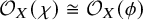 $\mathcal O_X(\chi )\cong \mathcal O_X(\phi )$
for some
$\mathcal O_X(\chi )\cong \mathcal O_X(\phi )$
for some
 $\phi \in {\mathrm {CP}}(\Sigma _X)$
. This implies
$\phi \in {\mathrm {CP}}(\Sigma _X)$
. This implies
 $\chi -\phi \in \operatorname {\mathrm {Aff}}_{\Sigma _X}(\Sigma _X)$
and hence
$\chi -\phi \in \operatorname {\mathrm {Aff}}_{\Sigma _X}(\Sigma _X)$
and hence
 $\chi \in {\mathrm {CP}}(\Sigma _X)$
because every affine function is combinatorially principal.
$\chi \in {\mathrm {CP}}(\Sigma _X)$
because every affine function is combinatorially principal.
5 Tropicalization of
$\psi $
classes

We turn our attention to the tautological cotangent line bundle to a section of a family of curves and study its tropicalization.
5.1 Tropicalization of the cotangent line bundle
In [Reference Cavalieri, Gross and Markwig6, Definition 6.16], tropical
 $\psi $
classes are defined as first Chern classes of certain torsors over the sheaf of affine functions of the base of a family of tropical curves. In this section we develop language and describe suitable conditions that allow us to compare the tropicalization of the i-th cotangent line bundle with the torsors above.
$\psi $
classes are defined as first Chern classes of certain torsors over the sheaf of affine functions of the base of a family of tropical curves. In this section we develop language and describe suitable conditions that allow us to compare the tropicalization of the i-th cotangent line bundle with the torsors above.
Definition 5.1. Let
 $\Sigma $
be a cone complex with a sheaf of affine functions
$\Sigma $
be a cone complex with a sheaf of affine functions
 $\operatorname {\mathrm {Aff}}_\Sigma $
, let
$\operatorname {\mathrm {Aff}}_\Sigma $
, let
 ${ \mathtt U}\subseteq \overline \Sigma $
be an open subcomplex, and let
${ \mathtt U}\subseteq \overline \Sigma $
be an open subcomplex, and let
 $\phi \in {\mathrm {sPL}}(\Sigma \cap { \mathtt U})$
. We define the sheaf
$\phi \in {\mathrm {sPL}}(\Sigma \cap { \mathtt U})$
. We define the sheaf
 $\operatorname {\mathrm {Aff}}_{ \mathtt U}(\phi )$
by
$\operatorname {\mathrm {Aff}}_{ \mathtt U}(\phi )$
by
for open subsets
 ${ \mathtt V}\subseteq { \mathtt U}$
. Note that
${ \mathtt V}\subseteq { \mathtt U}$
. Note that
 $\operatorname {\mathrm {Aff}}_{ \mathtt U}(\phi )$
is a pseudo-torsor over
$\operatorname {\mathrm {Aff}}_{ \mathtt U}(\phi )$
is a pseudo-torsor over
 $\operatorname {\mathrm {Aff}}_{ \mathtt U}$
, that is it is a torsor whenever it is nonempty. If
$\operatorname {\mathrm {Aff}}_{ \mathtt U}$
, that is it is a torsor whenever it is nonempty. If
 $\operatorname {\mathrm {Aff}}_{ \mathtt U}(\phi )$
is a torsor, it defines a tropical line bundle, which we also denote by
$\operatorname {\mathrm {Aff}}_{ \mathtt U}(\phi )$
is a torsor, it defines a tropical line bundle, which we also denote by
 $\operatorname {\mathrm {Aff}}_{ \mathtt U}(\phi )$
by abuse of notation.
$\operatorname {\mathrm {Aff}}_{ \mathtt U}(\phi )$
by abuse of notation.
Proposition 5.2. Let X be a toroidal variety, let
 $\phi \in {\mathrm {sPL}}(\Sigma _X)$
and let
$\phi \in {\mathrm {sPL}}(\Sigma _X)$
and let
 ${ \mathtt U}\subseteq \overline \Sigma _X$
. If
${ \mathtt U}\subseteq \overline \Sigma _X$
. If
 $\operatorname {\mathrm {Aff}}_{ \mathtt U}(\phi )$
is a tropical line bundle, then
$\operatorname {\mathrm {Aff}}_{ \mathtt U}(\phi )$
is a tropical line bundle, then
 ${\mathtt {Trop}}(\mathcal O_X(\phi ))\vert _{ \mathtt U}$
is a tropical line bundle as well and
${\mathtt {Trop}}(\mathcal O_X(\phi ))\vert _{ \mathtt U}$
is a tropical line bundle as well and
 $$ \begin{align} {\mathtt{Trop}}(\mathcal O_X(\phi))\vert_{ \mathtt U} \cong \operatorname{\mathrm{Aff}}_{ \mathtt U}(\phi) \end{align} $$
Proof. By Proposition 4.4,
 ${\mathtt {Trop}}(\mathcal O_X(\phi ))\vert _{ \mathtt U}$
is a tropical line bundle if and only if for every cell
${\mathtt {Trop}}(\mathcal O_X(\phi ))\vert _{ \mathtt U}$
is a tropical line bundle if and only if for every cell
 $\sigma /\tau $
of
$\sigma /\tau $
of
 ${ \mathtt U}$
there exists
${ \mathtt U}$
there exists
 $\phi _{\sigma /\tau }\in {\mathrm {sPL}}(\overline \Sigma ^{\sigma /\tau }_X)$
with
$\phi _{\sigma /\tau }\in {\mathrm {sPL}}(\overline \Sigma ^{\sigma /\tau }_X)$
with
 $$ \begin{align} \mathcal O_{X_\sigma}(\phi_{\sigma/\tau}+\phi)\vert_{V(\sigma)}\cong \mathcal O_{V(\sigma)} \; \end{align} $$
the collection of all the
 $-\phi _{\sigma /\tau }$
’s generates the pseudo-torsor
$-\phi _{\sigma /\tau }$
’s generates the pseudo-torsor
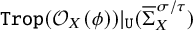 ${\mathtt {Trop}}(\mathcal O_X(\phi ))\vert _{{ \mathtt U}}(\overline \Sigma ^{\sigma /\tau }_X)$
of local affine sections. By definition of
${\mathtt {Trop}}(\mathcal O_X(\phi ))\vert _{{ \mathtt U}}(\overline \Sigma ^{\sigma /\tau }_X)$
of local affine sections. By definition of
 $\operatorname {\mathrm {Aff}}_{\overline \Sigma _X}$
, equation (5.3) means that
$\operatorname {\mathrm {Aff}}_{\overline \Sigma _X}$
, equation (5.3) means that
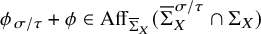 $\phi _{\sigma /\tau }+\phi \in \operatorname {\mathrm {Aff}}_{\overline \Sigma _X}(\overline \Sigma _X^{\sigma /\tau }\cap \Sigma _X)$
, which is equivalent to
$\phi _{\sigma /\tau }+\phi \in \operatorname {\mathrm {Aff}}_{\overline \Sigma _X}(\overline \Sigma _X^{\sigma /\tau }\cap \Sigma _X)$
, which is equivalent to
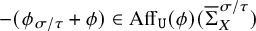 $-(\phi _{\sigma /\tau }+\phi )\in \operatorname {\mathrm {Aff}}_{ \mathtt U}(\phi )(\overline \Sigma _X^{\sigma /\tau })$
. The
$-(\phi _{\sigma /\tau }+\phi )\in \operatorname {\mathrm {Aff}}_{ \mathtt U}(\phi )(\overline \Sigma _X^{\sigma /\tau })$
. The
 $\operatorname {\mathrm {Aff}}_{{ \mathtt U}}(\overline \Sigma ^{\sigma /\tau }_X)$
-equivariant map
$\operatorname {\mathrm {Aff}}_{{ \mathtt U}}(\overline \Sigma ^{\sigma /\tau }_X)$
-equivariant map
 $$ \begin{align} {\mathtt{Trop}}(\mathcal O_X(\phi))\vert_{{ \mathtt U}}(\overline\Sigma^{\sigma/\tau}_X) \to \operatorname{\mathrm{Aff}}_{ \mathtt U}(\phi)(\overline\Sigma_X^{\sigma/\tau}), \;\; -\phi_{\sigma/\tau} \mapsto \chi = -\phi_{\sigma/\tau} -\phi \end{align} $$
is an isomorphism of pseudo-torsors. Therefore,
 ${\mathtt {Trop}}(\mathcal O_X(\phi ))\vert _{ \mathtt U}$
being a line bundle is equivalent to
${\mathtt {Trop}}(\mathcal O_X(\phi ))\vert _{ \mathtt U}$
being a line bundle is equivalent to
 $\operatorname {\mathrm {Aff}}_{ \mathtt U}(\phi )$
being a torsor, and the collection of maps (5.4) for
$\operatorname {\mathrm {Aff}}_{ \mathtt U}(\phi )$
being a torsor, and the collection of maps (5.4) for
 $\sigma /\tau \subseteq { \mathtt U}$
defines an isomorphism between
$\sigma /\tau \subseteq { \mathtt U}$
defines an isomorphism between
 ${\mathtt {Trop}}(\mathcal O_X(\phi ))\vert _{ \mathtt U}$
and
${\mathtt {Trop}}(\mathcal O_X(\phi ))\vert _{ \mathtt U}$
and
 $\operatorname {\mathrm {Aff}}_{ \mathtt U}(\phi )$
.
$\operatorname {\mathrm {Aff}}_{ \mathtt U}(\phi )$
.
We now apply these constructions to our main objects of interest: families of pointed curves and their tropicalizations.
Proposition 5.3. Let
 $\mathcal C\to \mathcal B$
be a tropicalizable family of n-marked stable curves with associated family of tropical curves
$\mathcal C\to \mathcal B$
be a tropicalizable family of n-marked stable curves with associated family of tropical curves
 $ \overline { \mathtt C}\to \overline { \mathtt B}$
, and let
$ \overline { \mathtt C}\to \overline { \mathtt B}$
, and let
 $1\leq i \leq n$
. Let
$1\leq i \leq n$
. Let
 $\phi $
be the piecewise linear function that has slope
$\phi $
be the piecewise linear function that has slope
 $1$
on the ray
$1$
on the ray
 $\rho _i$
corresponding to the i-th section
$\rho _i$
corresponding to the i-th section
 $s_i$
and is
$s_i$
and is
 $0$
on all cones not containing
$0$
on all cones not containing
 $\rho _i$
. Then there exists an isomorphism of pseudo
$\rho _i$
. Then there exists an isomorphism of pseudo
 $\operatorname {\mathrm {Aff}}_{\overline { \mathtt C}}$
-torsors
$\operatorname {\mathrm {Aff}}_{\overline { \mathtt C}}$
-torsors
 $$ \begin{align} \operatorname{\mathrm{Aff}}_{\overline{\mathtt C}}({\mathtt s}_i)\cong \operatorname{\mathrm{Aff}}_{\overline {\mathtt C}}(\phi) . \end{align} $$
Proof. Let
 ${ \mathtt U}\subseteq \overline {\mathtt C}$
be open. The sections of
${ \mathtt U}\subseteq \overline {\mathtt C}$
be open. The sections of
 $\operatorname {\mathrm {Aff}}_{\overline {\mathtt C}}(\phi )({ \mathtt U})$
are affine functions
$\operatorname {\mathrm {Aff}}_{\overline {\mathtt C}}(\phi )({ \mathtt U})$
are affine functions
 $\chi $
on
$\chi $
on
 ${ \mathtt U}\cap \mathtt C$
for which
${ \mathtt U}\cap \mathtt C$
for which
 $\chi +\phi $
can be extended continuously to
$\chi +\phi $
can be extended continuously to
 ${ \mathtt U}$
. Since
${ \mathtt U}$
. Since
 $\phi $
has slope
$\phi $
has slope
 $1$
on
$1$
on
 $\rho _i$
and vanishes on cones that do not contain
$\rho _i$
and vanishes on cones that do not contain
 $\rho _i$
, this is equivalent to saying that
$\rho _i$
, this is equivalent to saying that
 $\chi $
extends continuously to
$\chi $
extends continuously to
 ${ \mathtt U}\setminus {\mathtt s}_i$
and has slope
${ \mathtt U}\setminus {\mathtt s}_i$
and has slope
 $-1$
in the direction of
$-1$
in the direction of
 $\rho _i$
near
$\rho _i$
near
 ${\mathtt s}_i$
. By Definition 3.10, the continuous extension of
${\mathtt s}_i$
. By Definition 3.10, the continuous extension of
 $\chi $
to
$\chi $
to
 ${ \mathtt U}\setminus {\mathtt s}_i$
is automatically affine on
${ \mathtt U}\setminus {\mathtt s}_i$
is automatically affine on
 ${ \mathtt U}\setminus {\mathtt s}_i$
. We conclude that
${ \mathtt U}\setminus {\mathtt s}_i$
. We conclude that
 $\operatorname {\mathrm {Aff}}_{\overline {\mathtt C}}(\phi )({ \mathtt U})$
is in natural bijection with the subset of
$\operatorname {\mathrm {Aff}}_{\overline {\mathtt C}}(\phi )({ \mathtt U})$
is in natural bijection with the subset of
 $\operatorname {\mathrm {Aff}}_{\overline { \mathtt C}}({ \mathtt U}\setminus {\mathtt s}_i)$
of affine functions that approach
$\operatorname {\mathrm {Aff}}_{\overline { \mathtt C}}({ \mathtt U}\setminus {\mathtt s}_i)$
of affine functions that approach
 ${\mathtt s}_i$
with slope
${\mathtt s}_i$
with slope
 $-1$
. But this set equals
$-1$
. But this set equals
 $\operatorname {\mathrm {Aff}}_{\overline { \mathtt C}}({\mathtt s}_i)({ \mathtt U})$
by definition.
$\operatorname {\mathrm {Aff}}_{\overline { \mathtt C}}({\mathtt s}_i)({ \mathtt U})$
by definition.
Definition 5.4. Let
 $\mathcal C \to \mathcal B$
be a tropicalizable family of n-marked stable curves with tropicalization
$\mathcal C \to \mathcal B$
be a tropicalizable family of n-marked stable curves with tropicalization
 $\overline {{ \mathtt C}}\to \overline { \mathtt B}$
. If
$\overline {{ \mathtt C}}\to \overline { \mathtt B}$
. If
 $\operatorname {\mathrm {Aff}}_{\overline {{ \mathtt C}}}({\mathtt s}_i)$
is a tropical line bundle, we define the i-th tropical cotangent bundle analogously to [Reference Cavalieri, Gross and Markwig6, Definition 6.16]:
$\operatorname {\mathrm {Aff}}_{\overline {{ \mathtt C}}}({\mathtt s}_i)$
is a tropical line bundle, we define the i-th tropical cotangent bundle analogously to [Reference Cavalieri, Gross and Markwig6, Definition 6.16]:
where
 ${\mathtt s}_i={\mathtt {Trop}}(s_i)$
is the tropicalization of the i-th section
${\mathtt s}_i={\mathtt {Trop}}(s_i)$
is the tropicalization of the i-th section
Theorem 5.5. With setup and notation as in Definition 5.4, assume
 $\operatorname {\mathrm {Aff}}_{\overline {{ \mathtt C}}}({\mathtt s}_i)$
is a tropical line bundle. Then
$\operatorname {\mathrm {Aff}}_{\overline {{ \mathtt C}}}({\mathtt s}_i)$
is a tropical line bundle. Then ![]() tropicalizes to a tropical line bundle and we have
tropicalizes to a tropical line bundle and we have
Proof. Let
 $\phi $
be the function on
$\phi $
be the function on
 $\mathtt C$
that has slope
$\mathtt C$
that has slope
 $1$
on the ray
$1$
on the ray
 $\rho _i$
corresponding to
$\rho _i$
corresponding to
 $s_i$
and is
$s_i$
and is
 $0$
on all cones of
$0$
on all cones of
 $\mathtt C$
that do not contain
$\mathtt C$
that do not contain
 $\rho _i$
. By Proposition 5.3, we have
$\rho _i$
. By Proposition 5.3, we have
 $\operatorname {\mathrm {Aff}}_{\overline {\mathtt C}}(\phi )\cong \operatorname {\mathrm {Aff}}_{\overline {\mathtt C}}({\mathtt s}_i)$
. Using the assumption that
$\operatorname {\mathrm {Aff}}_{\overline {\mathtt C}}(\phi )\cong \operatorname {\mathrm {Aff}}_{\overline {\mathtt C}}({\mathtt s}_i)$
. Using the assumption that
 $\operatorname {\mathrm {Aff}}_{\overline {\mathtt C}}({\mathtt s}_i)$
is a tropical line bundle, we conclude that
$\operatorname {\mathrm {Aff}}_{\overline {\mathtt C}}({\mathtt s}_i)$
is a tropical line bundle, we conclude that
 $\operatorname {\mathrm {Aff}}_{\overline {\mathtt C}}(\phi )$
is a tropical line bundle as well. Applying Proposition 5.2, we see that the bundle
$\operatorname {\mathrm {Aff}}_{\overline {\mathtt C}}(\phi )$
is a tropical line bundle as well. Applying Proposition 5.2, we see that the bundle
 $\mathcal O_{\mathcal C}(s_i)\cong \mathcal O_{\mathcal C}(\phi )$
is tropicalizable and that the second isomorphism in the chain of isomorphisms
$\mathcal O_{\mathcal C}(s_i)\cong \mathcal O_{\mathcal C}(\phi )$
is tropicalizable and that the second isomorphism in the chain of isomorphisms
 $$ \begin{align} {\mathtt{Trop}}(\mathcal O_{\mathcal C}(s_i))\cong {\mathtt{Trop}}(\mathcal O_{\mathcal C}(\phi)) \cong \operatorname{\mathrm{Aff}}_{\overline { \mathtt C}}(\phi)\cong \operatorname{\mathrm{Aff}}_{\overline { \mathtt C}}({\mathtt s}_i) \end{align} $$
exists, the other ones being evident. Dualizing and applying Proposition 4.5 to the section
 $s_i$
then shows that
$s_i$
then shows that ![]() is defined and that we have a sequence of isomorphisms
is defined and that we have a sequence of isomorphisms

5.2 Tropicalizations of Cycles and Tropical Cycles
In order to translate Theorem 5.5 into a statement about
 $\psi $
classes, we need to take the first Chern class of a tropical line bundle. In this section we present the necessary bits of tropical intersection theory for this task. Similar definitions and constructions appeared in [Reference Cavalieri, Gross and Markwig6, Section 6]; here we present them in the slightly larger generality needed for the current context.
$\psi $
classes, we need to take the first Chern class of a tropical line bundle. In this section we present the necessary bits of tropical intersection theory for this task. Similar definitions and constructions appeared in [Reference Cavalieri, Gross and Markwig6, Section 6]; here we present them in the slightly larger generality needed for the current context.
Definition 5.6. Let X be a complete toroidal variety with associated complex
 $\Sigma _X$
, and let
$\Sigma _X$
, and let
 $c\in A^\ast (X)$
. Then the tropicalization of c is given by the weight
$c\in A^\ast (X)$
. Then the tropicalization of c is given by the weight
Proposition 5.7. Let X be an n-dimensional complete toroidal variety and let
 $c\in A^k(X)$
. Then the
$c\in A^k(X)$
. Then the
 $(n-k)$
-weight
$(n-k)$
-weight
 ${\mathtt {Trop}}(c)$
is balanced.
${\mathtt {Trop}}(c)$
is balanced.
Proof. Balancing can be checked locally around each cone
 $\sigma \in \Sigma _{X}$
of dimension
$\sigma \in \Sigma _{X}$
of dimension
 $n-k-1$
. The weight
$n-k-1$
. The weight
 ${\mathtt {Trop}}_X(c)$
induces a weight on
${\mathtt {Trop}}_X(c)$
induces a weight on
 $\Sigma ^\sigma _{X}/\sigma $
and this weight coincides with
$\Sigma ^\sigma _{X}/\sigma $
and this weight coincides with
 ${\mathtt {Trop}}(\iota ^*c)$
, where
${\mathtt {Trop}}(\iota ^*c)$
, where
 $\iota \colon V(\sigma )\to X$
is the inclusion. Because the functions near
$\iota \colon V(\sigma )\to X$
is the inclusion. Because the functions near
 $\sigma $
that vanish on
$\sigma $
that vanish on
 $\sigma $
are pulled back from
$\sigma $
are pulled back from
 $\Sigma _{X}^\sigma /\sigma \cong \Sigma _{V(\sigma )}$
by Lemma 3.11, it suffices to prove that
$\Sigma _{X}^\sigma /\sigma \cong \Sigma _{V(\sigma )}$
by Lemma 3.11, it suffices to prove that
 ${\mathtt {Trop}}(\iota ^*c)$
is balanced on
${\mathtt {Trop}}(\iota ^*c)$
is balanced on
 $\Sigma _{V(\sigma )}$
. We have reduced to the case where
$\Sigma _{V(\sigma )}$
. We have reduced to the case where
 $k=n-1$
and
$k=n-1$
and
 ${\mathtt {Trop}}(c)$
is
${\mathtt {Trop}}(c)$
is
 $1$
-dimensional. Let
$1$
-dimensional. Let
 $\phi \in \operatorname {\mathrm {Aff}}_{\Sigma _X}(\Sigma _X)$
. We have
$\phi \in \operatorname {\mathrm {Aff}}_{\Sigma _X}(\Sigma _X)$
. We have
 $$ \begin{align} \sum_{\rho\in \Sigma_X(1)}\mathrm{slope}_\rho(\phi) c(\rho) = \int_X c\cdot \left(\sum_{\rho\in\Sigma_X(1)} \mathrm{slope}_\rho(\phi) [V(\rho)]\right) = \int_X c \cdot c_1(\mathcal O_X(\phi)) = 0 , \end{align} $$
where the last equality follows from the fact that
 $\mathcal O_X(\phi )$
is trivial because
$\mathcal O_X(\phi )$
is trivial because
 $\phi $
is affine. The vanishing of the first term in (5.11) shows balancing, thus concluding the proof.
$\phi $
is affine. The vanishing of the first term in (5.11) shows balancing, thus concluding the proof.
Applying Proposition 5.7 to the unity of the Chow ring, we obtain a tropical fundamental class.
Corollary 5.8. Let X be an n-dimensional complete toroidal variety. The constant weight with value
 $1$
on the n-dimensional cones of
$1$
on the n-dimensional cones of
 $\Sigma _X$
is balanced. We denote by
$\Sigma _X$
is balanced. We denote by
 $[\Sigma _X]$
the corresponding tropical cycle.
$[\Sigma _X]$
the corresponding tropical cycle.
Proof. The constant weight
 $1$
on n-dimensional cones is equal to
$1$
on n-dimensional cones is equal to
 ${\mathtt {Trop}}_X(1)$
, where
${\mathtt {Trop}}_X(1)$
, where
 $1\in A^0(X)$
is the multiplicative identity of the Chow ring. The assertion follows from Proposition 5.7.
$1\in A^0(X)$
is the multiplicative identity of the Chow ring. The assertion follows from Proposition 5.7.
Definition 5.9. For a complete toroidal variety X of dimension n we call the tropical cycle represented by the balanced n-weight with value
 $1$
on all n-dimensional cones of
$1$
on all n-dimensional cones of
 $\Sigma _X$
the fundamental class of
$\Sigma _X$
the fundamental class of
 $\Sigma _X$
and denote it by
$\Sigma _X$
and denote it by
 $[\Sigma _X]$
The final missing ingredient to show that tropicalizations of
 $\psi $
classes coincide with tropical
$\psi $
classes coincide with tropical
 $\psi $
classes operationally is the compatibility of tropicalization with intersections with first Chern classes of line bundles. This is the content of the following proposition, which generalizes [Reference Gross11, Proposition 4.13].
$\psi $
classes operationally is the compatibility of tropicalization with intersections with first Chern classes of line bundles. This is the content of the following proposition, which generalizes [Reference Gross11, Proposition 4.13].
Proposition 5.10. Let X be a complete toroidal variety with cone complex
 $\Sigma _X$
, let
$\Sigma _X$
, let
 $c\in A^k(X)$
, and let
$c\in A^k(X)$
, and let
 $\mathcal L$
be a tropicalizable line bundle on X with tropicalization
$\mathcal L$
be a tropicalizable line bundle on X with tropicalization
 $\mathtt L$
on
$\mathtt L$
on
 $\overline \Sigma _X$
. Then we have
$\overline \Sigma _X$
. Then we have
 $$ \begin{align} [{\mathtt{Trop}}_X(c_1(\mathcal L) \cdot c)] = c_1(\mathtt L) \frown [{\mathtt{Trop}}_X(c)] \end{align} $$
Proof. By Corollary 4.7, there exists a function
 $\phi \in {\mathrm {CP}}(\Sigma _X)$
with
$\phi \in {\mathrm {CP}}(\Sigma _X)$
with
 $\mathcal L\cong \mathcal O_X(\phi )$
. Let
$\mathcal L\cong \mathcal O_X(\phi )$
. Let
 $\tau \in \Sigma _X$
be a cone of dimension
$\tau \in \Sigma _X$
be a cone of dimension
 $n-k-1$
, where
$n-k-1$
, where
 $n=\dim (X)$
. We need to show that the weights on both sides of (5.12) have the same value on
$n=\dim (X)$
. We need to show that the weights on both sides of (5.12) have the same value on
 $\tau $
. Since
$\tau $
. Since
 $\phi \in {\mathrm {CP}}(\Sigma _X)$
, we may assume that
$\phi \in {\mathrm {CP}}(\Sigma _X)$
, we may assume that
 $\phi \vert _\tau =0$
. We denote by
$\phi \vert _\tau =0$
. We denote by
 $\phi ^\tau $
the induced function on
$\phi ^\tau $
the induced function on
 $\Sigma _X^\tau /\tau $
. Then we have
$\Sigma _X^\tau /\tau $
. Then we have
 $\mathcal O_X(\phi )\vert _{V(\tau )}\cong \mathcal O_{V(\tau )}(\phi ^\tau )$
and thus
$\mathcal O_X(\phi )\vert _{V(\tau )}\cong \mathcal O_{V(\tau )}(\phi ^\tau )$
and thus
 $$ \begin{align} c_1(\mathcal L)\cdot [V(\tau)] = \sum_{\sigma} \mathrm{slope}_{\sigma/\tau}(\phi^\tau) [V(\sigma)] \quad \text{in }A^{k+1}(X) , \end{align} $$
where the sum is taken over all
 $(n-k)$
-dimensional cones of
$(n-k)$
-dimensional cones of
 $\Sigma _X$
containing
$\Sigma _X$
containing
 $\tau $
. Therefore, we have
$\tau $
. Therefore, we have
 $$ \begin{align} {\mathtt{Trop}}_X(c_1(\mathcal L)\cdot c)(\tau)= \int_{V(\tau)} c_1(\mathcal L)\cdot c = \sum_{\sigma} \mathrm{slope}_{\sigma/\tau}(\phi^\tau) {\mathtt{Trop}}_X(c)(\sigma) . \end{align} $$
By Proposition 4.4, the function
 $-\phi ^\tau $
is the local equation on
$-\phi ^\tau $
is the local equation on
 $\overline \Sigma ^{\tau /\tau }$
for a tropical Cartier divisor whose associated line bundle is
$\overline \Sigma ^{\tau /\tau }$
for a tropical Cartier divisor whose associated line bundle is
 ${ \mathtt L}$
. Therefore, the last term in (5.14) equals the local expression for the weight at
${ \mathtt L}$
. Therefore, the last term in (5.14) equals the local expression for the weight at
 $\tau $
of
$\tau $
of
 $c_1( \mathtt L)\ \frown [{\mathtt {Trop}}_X(c)]$
(compare with (2.3)).
$c_1( \mathtt L)\ \frown [{\mathtt {Trop}}_X(c)]$
(compare with (2.3)).
Corollary 5.11. Let
 $\mathcal C\to \mathcal B$
be a tropicalizable family of n-marked stable curves with tropicalization
$\mathcal C\to \mathcal B$
be a tropicalizable family of n-marked stable curves with tropicalization
 $ \mathtt {C}\to \mathtt {B}$
, and let
$ \mathtt {C}\to \mathtt {B}$
, and let
 $1\leq i \leq n$
. Assume
$1\leq i \leq n$
. Assume
 $\operatorname {\mathrm {Aff}}_{\overline {\mathtt C}}(-{\mathtt s}_i)$
is a tropical line bundle. Then
$\operatorname {\mathrm {Aff}}_{\overline {\mathtt C}}(-{\mathtt s}_i)$
is a tropical line bundle. Then
 $$ \begin{align} {\mathtt{Trop}}(\psi_i) = \psi_i^{\mathtt{trop}} . \end{align} $$
6 An extended example in genus one
This section is dedicated to an extended example of the theory set-up in the previous part of the paper. We study two
 $2$
-dimensional families of genus-one curves with two marked points. They arise from a single family of admissible covers by forgetting different subsets of the marked ramification. We exhibit the tropical
$2$
-dimensional families of genus-one curves with two marked points. They arise from a single family of admissible covers by forgetting different subsets of the marked ramification. We exhibit the tropical
 $\psi $
class as a
$\psi $
class as a
 $1$
-dimensional cycle on the base and show it is the tropicalization of the corresponding algebraic cycle.
$1$
-dimensional cycle on the base and show it is the tropicalization of the corresponding algebraic cycle.
6.1 Algebraic set-up
We consider the (algebraic) moduli space of admissible covers
 $$ \begin{align} \overline{Adm}_{1\to 0}((3), (2,1)^4) . \end{align} $$
Its closed points parameterize degree-
 $3$
admissible covers of a rational curve, where one branch point is the image of exactly one ramification point (of order
$3$
admissible covers of a rational curve, where one branch point is the image of exactly one ramification point (of order
 $3$
), whereas the other four branch points are simple: their inverse image consists of two points, one unramified and one simply ramified. There is a natural branch morphism:
$3$
), whereas the other four branch points are simple: their inverse image consists of two points, one unramified and one simply ramified. There is a natural branch morphism:
 $$ \begin{align} \mathrm{br}:\overline{Adm}_{1\to 0}((3), (2,1)^4)\to \overline{\mathcal{M}}_{0,5} , \end{align} $$
recording the target of the cover together with the marked branch points. It is a finite morphism of degree
 $9$
. We adopt the convention that all inverse images of branch points are marked, and therefore we have a natural source morphism:
$9$
. We adopt the convention that all inverse images of branch points are marked, and therefore we have a natural source morphism:
 $$ \begin{align} \mathrm{src}:\overline{Adm}_{1\to 0}((3), (2,1)^4)\to \overline{\mathcal{M}}_{1,9} . \end{align} $$
Let
 $r_1: \overline {\mathcal {M}}_{1,9} \to \overline {\mathcal {M}}_{1,2}$
(resp.
$r_1: \overline {\mathcal {M}}_{1,9} \to \overline {\mathcal {M}}_{1,2}$
(resp.
 $r_2$
) be the morphism that forgets all marks except (the one corresponding to) the point of triple ramification and one of the unramified (resp. simply ramified) marked points. We adopt the notation that the first mark in
$r_2$
) be the morphism that forgets all marks except (the one corresponding to) the point of triple ramification and one of the unramified (resp. simply ramified) marked points. We adopt the notation that the first mark in
 $\overline {\mathcal {M}}_{1,2}$
is the point of triple ramification of the cover.
$\overline {\mathcal {M}}_{1,2}$
is the point of triple ramification of the cover.
One may compose
 $r_i\circ \mathrm {src}$
, and pull-back the universal family of
$r_i\circ \mathrm {src}$
, and pull-back the universal family of
 $\overline {\mathcal {M}}_{1,2}$
to obtain a family of genus-one, two-marked curves:
$\overline {\mathcal {M}}_{1,2}$
to obtain a family of genus-one, two-marked curves:

We denote the space of admissible covers by
 $\mathcal B_i$
both to shorten the notation and to emphasize that we think of it as the base of a family of curves, determined by the map
$\mathcal B_i$
both to shorten the notation and to emphasize that we think of it as the base of a family of curves, determined by the map
 $\varphi _i: \mathcal B_i\to \overline {\mathcal {M}}_{1,2}$
.
$\varphi _i: \mathcal B_i\to \overline {\mathcal {M}}_{1,2}$
.
Lemma 6.1. We determine the degree of the maps
 $\varphi _1, \varphi _2$
.
$\varphi _1, \varphi _2$
.
-
1. The degree of
$\varphi _1: \mathcal B_1\to \overline {\mathcal {M}}_{1,2}$
is equal to
$24$
, that is, (6.5)
$$ \begin{align} \varphi_{1, \ast}([\mathcal B_1]) = 24[\overline{\mathcal{M}}_{1,2}] . \end{align} $$
-
2. The degree of
$\varphi _2: \mathcal B_2\to \overline {\mathcal {M}}_{1,2}$
is equal to
$6$
, that is, (6.6)
$$ \begin{align} \varphi_{2, \ast}([\mathcal B_2]) = 6[\overline{\mathcal{M}}_{1,2}] . \end{align} $$


Proof. Consider a general point
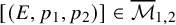 $[(E, p_1, p_2)]\in \overline {\mathcal {M}}_{1,2}$
, that is, a smooth genus-one curve with two marked points. A map
$[(E, p_1, p_2)]\in \overline {\mathcal {M}}_{1,2}$
, that is, a smooth genus-one curve with two marked points. A map ![]() in the inverse image of
in the inverse image of
 $[(E, p_1, p_2)]$
via
$[(E, p_1, p_2)]$
via
 $\varphi _1$
corresponds to a principal divisor of the form
$\varphi _1$
corresponds to a principal divisor of the form
 $3p_1 -p_2 - 2x$
, where x is a point of E to be determined. One can solve for x in
$3p_1 -p_2 - 2x$
, where x is a point of E to be determined. One can solve for x in
 $Jac(E) \cong E$
, and find that there are four solutions (pick any particular solution and then one can add any one of the four two-torsion points of
$Jac(E) \cong E$
, and find that there are four solutions (pick any particular solution and then one can add any one of the four two-torsion points of
 $Jac(E)$
). There are therefore four distinct maps that have triple ramification at
$Jac(E)$
). There are therefore four distinct maps that have triple ramification at
 $p_1$
and are unramified at
$p_1$
and are unramified at
 $p_2$
(but where
$p_2$
(but where
 $p_2$
is the inverse image of a branch point). Generically, for each of these maps there are
$p_2$
is the inverse image of a branch point). Generically, for each of these maps there are
 $3!$
ways to label the remaining simple ramification points, and once that is done the remaining marks are determined. There is therefore a total of
$3!$
ways to label the remaining simple ramification points, and once that is done the remaining marks are determined. There is therefore a total of
 $24$
inverse images, which proves
$24$
inverse images, which proves
 $(1)$
.
$(1)$
.
Similarly, to determine the inverse images via
 $\varphi _2$
of
$\varphi _2$
of
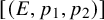 $[(E, p_1, p_2)]$
one must solve the equation
$[(E, p_1, p_2)]$
one must solve the equation
 $3p_1-2p_2-x = 0 \in Jac(E)$
, which has a unique solution. There is only one map with triple ramification at
$3p_1-2p_2-x = 0 \in Jac(E)$
, which has a unique solution. There is only one map with triple ramification at
 $p_1$
and simple ramification at
$p_1$
and simple ramification at
 $p_2$
and
$p_2$
and
 $3! = 6$
ways to label the remaining simple ramification points, for a total of six inverse images. This proves (2).
$3! = 6$
ways to label the remaining simple ramification points, for a total of six inverse images. This proves (2).
We conclude the description of the algebraic set up by spelling out the relation between the class
 $\psi _1$
on
$\psi _1$
on
 $\overline {\mathcal {M}}_{1,2}$
and the pushforward of the class
$\overline {\mathcal {M}}_{1,2}$
and the pushforward of the class
 $\psi _1$
on
$\psi _1$
on
 $\mathcal B_i$
via the morphism
$\mathcal B_i$
via the morphism
 $\varphi _i$
.
$\varphi _i$
.
Lemma 6.2. Denote by W the class of the Weierstrass divisor in
 $\overline {\mathcal {M}}_{1,2}$
(parameterizing curves of genus one where both marks are Weierstrass points of the same
$\overline {\mathcal {M}}_{1,2}$
(parameterizing curves of genus one where both marks are Weierstrass points of the same
 $g_2^1$
). We have the following equalities in
$g_2^1$
). We have the following equalities in
 $A^1(\overline {\mathcal {M}}_{1,2})$
:
$A^1(\overline {\mathcal {M}}_{1,2})$
:
 $$ \begin{align} \varphi_{1, \ast}(\psi_1) &= 24 \psi_1 , \end{align} $$
 $$ \begin{align} \varphi_{2, \ast}(\psi_1) &= 6 (\psi_1 +W) . \end{align} $$
Proof. Since we need to pull-back and push-forward classes on different spaces that are all called
 $\psi _1$
on their respective space, we adopt the convention of just letting the context indicate which class is which. There are two fundamental pull-back relations that we will be using:
$\psi _1$
on their respective space, we adopt the convention of just letting the context indicate which class is which. There are two fundamental pull-back relations that we will be using:
 $$ \begin{align} \psi_1 = r_i^\ast(\psi_1) + D_i , \end{align} $$
where
 $D_i$
denotes the sum of all rational tails boundary divisors of
$D_i$
denotes the sum of all rational tails boundary divisors of
 $\overline {\mathcal {M}}_{1,9}$
parameterizing nodal curves where the mark
$\overline {\mathcal {M}}_{1,9}$
parameterizing nodal curves where the mark
 $1$
lies on the rational tail, and the mark
$1$
lies on the rational tail, and the mark
 $2$
lies on the genus-one component of the curve. This relation follows from iterated application of the standard pull-back relation for
$2$
lies on the genus-one component of the curve. This relation follows from iterated application of the standard pull-back relation for
 $\psi $
classes along forgetful morphisms (see, e.g., [Reference Kock19, Lemma 1.3.1]). With respect to the morphism
$\psi $
classes along forgetful morphisms (see, e.g., [Reference Kock19, Lemma 1.3.1]). With respect to the morphism
 $\mathrm {src}$
,
$\mathrm {src}$
,
 $$ \begin{align} \psi_1 = \mathrm{src}^\ast(\psi_1) , \end{align} $$
follows from the fact that the first mark is a point of full ramification for the cover, that can therefore not live in an unstable component of the source curve of the admissible cover.
Next we analyze the divisor
 $\mathrm {src}^\ast (D_i)$
. When
$\mathrm {src}^\ast (D_i)$
. When
 $i=1$
, that is, when the second mark corresponds to a nonramified point of the cover, then one may observe that the image of
$i=1$
, that is, when the second mark corresponds to a nonramified point of the cover, then one may observe that the image of
 $\mathrm {src}$
is disjoint from
$\mathrm {src}$
is disjoint from
 $D_1$
, and therefore
$D_1$
, and therefore
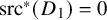 $\mathrm {src}^\ast (D_1) = 0$
.
$\mathrm {src}^\ast (D_1) = 0$
.
In the other case,
 $\mathrm {src}^\ast (D_2)$
is the sum of three irreducible boundary divisors in the space of admissible covers, depicted in Figure 7. They parameterize the same topological type of covers, and differ only in the labeling of the inverse images of the branch points.
$\mathrm {src}^\ast (D_2)$
is the sum of three irreducible boundary divisors in the space of admissible covers, depicted in Figure 7. They parameterize the same topological type of covers, and differ only in the labeling of the inverse images of the branch points.
A topological cartoon of the admissible covers parameterized by the general points of
 $\mathrm {src}^\ast (D_2)$
. The blue points are the marked points that get forgotten by the map
$\mathrm {src}^\ast (D_2)$
. The blue points are the marked points that get forgotten by the map
 $r_2$
, which we did not label to avoid cluttering the figure. There are three possible ways to order the pairs of blue points, giving rise to three irreducible components.
$r_2$
, which we did not label to avoid cluttering the figure. There are three possible ways to order the pairs of blue points, giving rise to three irreducible components.

The final step is to apply the projection formula. In the case
 $i=1$
, we have that
$i=1$
, we have that
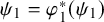 $\psi _1 = \varphi _1^\ast (\psi _1)$
, and we have shown that
$\psi _1 = \varphi _1^\ast (\psi _1)$
, and we have shown that
 $\varphi _1$
is a finite morphism of degree
$\varphi _1$
is a finite morphism of degree
 $24$
, from which (6.7) follows.
$24$
, from which (6.7) follows.
In the second case, we have
 $$ \begin{align} \varphi_{2,\ast}(\psi_1) = 6\psi_1 + \varphi_{2,\ast}(\mathrm{src}^\ast(D_2)) . \end{align} $$
One finally observes that each of the three boundary divisors comprising
 $\mathrm {src}^\ast (D_2)$
pushes forward to
$\mathrm {src}^\ast (D_2)$
pushes forward to
 $2W$
(the factor of
$2W$
(the factor of
 $2$
coming from the gluing ghost automorphisms of the node), thus yielding (6.8).
$2$
coming from the gluing ghost automorphisms of the node), thus yielding (6.8).
6.2 Tropical family
We consider the moduli space of tropical admissible covers as introduced in [Reference Caporaso3, Reference Cavalieri, Markwig and Ranganathan7]
 $$ \begin{align} \overline{Adm}^{{\mathtt{trop}}}_{1\to 0}((3), (2,1)^4) . \end{align} $$
It is a two-dimensional cone complex, with
 $20$
rays and
$20$
rays and
 $45$
two-dimensional cones which we call faces for simplicity. Forgetting the labeling of the five points on the target trees, one can group the rays into
$45$
two-dimensional cones which we call faces for simplicity. Forgetting the labeling of the five points on the target trees, one can group the rays into
 $4$
distinct types; similarly, the faces are grouped into
$4$
distinct types; similarly, the faces are grouped into
 $5$
types. The topological types of tropical covers corresponding to these types are depicted in Figure 8. We describe the various incidence properties of rays and faces.
$5$
types. The topological types of tropical covers corresponding to these types are depicted in Figure 8. We describe the various incidence properties of rays and faces.
The topological types of tropical covers corresponding to the rays and two-dimensional cones of
 $\overline {Adm}^{{\mathtt {trop}}}_{1\to 0}((3), (2,1)^4)$
. Types are labeled as in their description in Section 6.2. The color coding is meant to facilitate the understanding of the structure of the cone complex of tropical admissible covers, represented in Figure 9.
$\overline {Adm}^{{\mathtt {trop}}}_{1\to 0}((3), (2,1)^4)$
. Types are labeled as in their description in Section 6.2. The color coding is meant to facilitate the understanding of the structure of the cone complex of tropical admissible covers, represented in Figure 9.

Rays:
-
type ρa there are six rays of type
$\rho _a$
; each is adjacent to two faces of type
$\sigma _1$
, a face of type
$\sigma _4$
and one of type
$\sigma _5$
; -
type ρb there are six rays of type
$\rho _b$
; each is adjacent to two faces of type
$\sigma _2$
, two faces of type
$\sigma _3$
and one of type
$\sigma _5$
; -
type ρc there are four rays of type
$\rho _c$
; each is adjacent to three faces of type
$\sigma _1$
, and three faces of type
$\sigma _2$
; -
type ρd there are four rays of type
$\rho _d$
; each is adjacent to three faces of type
$\sigma _3$
.


Faces:
-
type σ1 there are twelve faces of type
$\sigma _1$
, each bounded by a ray of type
$\rho _a$
and one of type
$\rho _c$
; -
type σ2 there are twelve faces of type
$\sigma _2$
, each bounded by a ray of type
$\rho _b$
and one of type
$\rho _c$
; -
type σ3 there are twelve faces of type
$\sigma _3$
, each bounded by a ray of type
$\rho _b$
and one of type
$\rho _d$
; -
type σ4 there are three faces of type
$\sigma _4$
, each bounded by two rays of type
$\rho _a$
; -
type σ5 there are six faces of type
$\sigma _5$
, each bounded by a ray of type
$\rho _a$
and one of type
$\rho _b$
.


6.3 Tropicalization and the fundamentalish cycle.
The tropicalization of the Hurwitz space (compactified in the space of admissible covers) is a cone complex which may be naturally identified with the Berkovich skeleton of the analytic Hurwitz space. In [Reference Cavalieri, Markwig and Ranganathan7], the authors exhibit a natural tropicalization map
 $\mathtt T$
from the Berkovich analytic skeleton
$\mathtt T$
from the Berkovich analytic skeleton
 $\Sigma $
of the Hurwitz space (
$\Sigma $
of the Hurwitz space (
 $\Sigma $
agrees with the cone complex associated to the toroidal compactification given by the space of admissible covers) to the cone complex of tropical admissible covers. This map is a strict morphism of cone complexes, but in general it is not an isomorphism. Surjectivity fails if some tropical admissible cover is not dual to any algebraic one. This situation is detected by the vanishing of some local Hurwitz number associated to a vertex of some tropical admissible cover. Injectivity may fail for two reasons: multiple strata may give rise to the same topological type of tropical cover if they arise from the normalization of a singular locus in the space of admissible covers: this happens when in a tropical admissible cover, there are multiple edges mapping to a given edge of the target graph, and their expansion factors are not pairwise coprime. Alternatively, it may be that there are multiple algebraic covers of a component of the target curve: this situation is a bit more delicate and it is assessed by observing the local Hurwitz numbers and the automorphism factors around the vertices of a tropical admissible covers.
$\Sigma $
agrees with the cone complex associated to the toroidal compactification given by the space of admissible covers) to the cone complex of tropical admissible covers. This map is a strict morphism of cone complexes, but in general it is not an isomorphism. Surjectivity fails if some tropical admissible cover is not dual to any algebraic one. This situation is detected by the vanishing of some local Hurwitz number associated to a vertex of some tropical admissible cover. Injectivity may fail for two reasons: multiple strata may give rise to the same topological type of tropical cover if they arise from the normalization of a singular locus in the space of admissible covers: this happens when in a tropical admissible cover, there are multiple edges mapping to a given edge of the target graph, and their expansion factors are not pairwise coprime. Alternatively, it may be that there are multiple algebraic covers of a component of the target curve: this situation is a bit more delicate and it is assessed by observing the local Hurwitz numbers and the automorphism factors around the vertices of a tropical admissible covers.
The tropical source and target morphisms factor via the tropicalization map
 $\mathtt T$
; in the specific case we are studying they give rise to the following commutative diagram:
$\mathtt T$
; in the specific case we are studying they give rise to the following commutative diagram:

By the functoriality of tropicalization (Proposition 3.5), any (local, affine) linear function on
 $\overline {\mathcal {M}}_{1,9}^{\mathtt {trop}}$
(resp.
$\overline {\mathcal {M}}_{1,9}^{\mathtt {trop}}$
(resp.
 $ \overline {\mathcal {M}}_{0,5}^{\mathtt {trop}}$
) pulls-back via
$ \overline {\mathcal {M}}_{0,5}^{\mathtt {trop}}$
) pulls-back via
 $\mathtt {Src}$
(resp.
$\mathtt {Src}$
(resp.
 $\mathtt {Br}$
) to a linear function on the cone complex
$\mathtt {Br}$
) to a linear function on the cone complex
 $\Sigma $
of
$\Sigma $
of
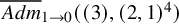 $\overline {Adm}_{1\to 0}((3), (2,1)^4)$
.
$\overline {Adm}_{1\to 0}((3), (2,1)^4)$
.
We declare that linear functions pulled back via
 $\mathtt {src}$
and
$\mathtt {src}$
and
 $\mathtt {br}$
are linear functions on the tropical moduli space
$\mathtt {br}$
are linear functions on the tropical moduli space
 $\overline {Adm}^{{\mathtt {trop}}}_{1\to 0}((3), (2,1)^4)$
. By the commutativity of (6.13) such a declaration is compatible with further pulling back via
$\overline {Adm}^{{\mathtt {trop}}}_{1\to 0}((3), (2,1)^4)$
. By the commutativity of (6.13) such a declaration is compatible with further pulling back via
 $\mathtt T$
. As a further consequence, any intersection-theoretic computation on
$\mathtt T$
. As a further consequence, any intersection-theoretic computation on
 $\Sigma $
involving cycles pulled back from source or target morphism may be reproduced, by the projection formula, on the moduli space
$\Sigma $
involving cycles pulled back from source or target morphism may be reproduced, by the projection formula, on the moduli space
 $\overline {Adm}^{{\mathtt {trop}}}_{1\to 0}((3), (2,1)^4)$
.
$\overline {Adm}^{{\mathtt {trop}}}_{1\to 0}((3), (2,1)^4)$
.
It is then necessary to study the push-forward of the fundamental class of
 $\Sigma $
via
$\Sigma $
via
 $\mathtt T$
. We have
$\mathtt T$
. We have
 $$ \begin{align} \mathtt T_\ast([\Sigma]) = \sum_\sigma \omega(\sigma) \sigma , \end{align} $$
where the sum runs over all top-dimensional cones of
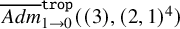 $\overline {Adm}^{{\mathtt {trop}}}_{1\to 0}((3), (2,1)^4)$
. The weight
$\overline {Adm}^{{\mathtt {trop}}}_{1\to 0}((3), (2,1)^4)$
. The weight
 $\omega (\sigma )$
, for a cone
$\omega (\sigma )$
, for a cone
 $\sigma $
parameterizing tropical admissible covers
$\sigma $
parameterizing tropical admissible covers
 $\Gamma \to \Delta $
of combinatorial type
$\Gamma \to \Delta $
of combinatorial type
 $\Theta $
is as in [Reference Cavalieri, Markwig and Ranganathan7, Definition 22] the product of the following factors:
$\Theta $
is as in [Reference Cavalieri, Markwig and Ranganathan7, Definition 22] the product of the following factors:
-
(W1) a factor of
$\frac {1}{|\operatorname {\mathrm {Aut}}_0(\Theta )|}$
, with
$\operatorname {\mathrm {Aut}}_0(\Theta )$
denoting automorphisms of the tropical cover fixing the source curve; -
(W2) a factor of local Hurwitz numbers
$\prod _{v\in V(\Gamma )} H(v)$
; -
(W3) a factor of
$\prod _{e\in E(\Delta )} w_e$
, where
$w_e$
is the product of the expansion factors above the edge e, divided by their LCM.


For the moduli space
 $\overline {Adm}^{{\mathtt {trop}}}_{1\to 0}((3), (2,1)^4)$
that we are studying, all local Hurwitz numbers appearing are nonzero, hence the map
$\overline {Adm}^{{\mathtt {trop}}}_{1\to 0}((3), (2,1)^4)$
that we are studying, all local Hurwitz numbers appearing are nonzero, hence the map
 $\mathtt T$
is surjective. Every time there are multiple edges mapping to an edge of a target graph, their expansion factors are pairwise coprime. All local Hurwitz numbers appearing are equal to one, except for two:
$\mathtt T$
is surjective. Every time there are multiple edges mapping to an edge of a target graph, their expansion factors are pairwise coprime. All local Hurwitz numbers appearing are equal to one, except for two:
-
• in the tropical cover parameterized by cone
$\sigma _4$
the genus-one vertex has local Hurwitz number equal to
$1/3$
; this corresponds to the unique genus-one curve admitting a degree
$3$
automorphism; -
• the central vertex in the tropical cover parameterized by cone
$\sigma _5$
has local Hurwitz number equal to
$2$
, corresponding to different labelings of the three unramified points: there are in fact six possible labelings, but a factor of three is divided out because of the automorphism of the cover.


The covers parameterized by cones of type
 $\sigma _3$
and
$\sigma _3$
and
 $\sigma _5$
have a group of automorphisms of order two, while all other types have no nontrivial automorphisms. This information is systematically collected in Table 1.
$\sigma _5$
have a group of automorphisms of order two, while all other types have no nontrivial automorphisms. This information is systematically collected in Table 1.
The factors computing the weights of two-dimensional cones in
 $\overline {Adm}^{{\mathtt {trop}}}_{1\to 0}((3), (2,1)^4)$
.
$\overline {Adm}^{{\mathtt {trop}}}_{1\to 0}((3), (2,1)^4)$
.

In conclusion, if we denote by
 $\sigma ^{\mathtt {tot}}_i$
the formal sum of all two-dimensional cones of type
$\sigma ^{\mathtt {tot}}_i$
the formal sum of all two-dimensional cones of type
 $\sigma _i$
, we obtain:
$\sigma _i$
, we obtain:
 $$ \begin{align} \mathtt T_\ast([\Sigma]) = \sigma^{\mathtt{tot}}_1+\sigma^{\mathtt{tot}}_2+\frac{1}{2}\sigma^{\mathtt{tot}}_3+\frac{1}{3}\sigma^{\mathtt{tot}}_4+\sigma^{\mathtt{tot}}_5 . \end{align} $$
The cycle in (6.15) plays the role of the fundamental class in the forthcoming computations, and we therefore dub it the fundamentalish cycle of the moduli space of tropical admissible covers.
6.4 The tropical
$\psi $
class

In this section we study the class
 $\psi _1$
, supported on the mark with expansion factor
$\psi _1$
, supported on the mark with expansion factor
 $3$
, in the two-dimensional family of tropical admissible covers introduced in the previous sections. Our first result is that the tropical
$3$
, in the two-dimensional family of tropical admissible covers introduced in the previous sections. Our first result is that the tropical
 $\psi $
class is in fact the tropicalization of the algebraic
$\psi $
class is in fact the tropicalization of the algebraic
 $\psi $
class.
$\psi $
class.
Proposition 6.3. Consider the families of genus-one,
 $9$
-marked algebraic and tropical curves given by the morphisms
$9$
-marked algebraic and tropical curves given by the morphisms
 $\mathrm {src}$
and
$\mathrm {src}$
and
 $\mathtt {src}$
introduced in the previous sections. Then we have the following equality of operational classes with
$\mathtt {src}$
introduced in the previous sections. Then we have the following equality of operational classes with ![]() -coefficients:
-coefficients:
 $$ \begin{align} \psi_1^{\mathtt{trop}} = {\mathtt{Trop}}(\psi_1) , \end{align} $$
where we have omitted explicitly writing the pull-back via the source morphism in order to not burden the notation unnecessarily.
Proof. By Corollary 5.11 it suffices to show that the affine structure on the family of tropical admissible covers induced by tropicalization contains enough information to define
 $\psi _1^{\mathtt {trop}}$
. In fact, as the desired equality has coefficients in
$\psi _1^{\mathtt {trop}}$
. In fact, as the desired equality has coefficients in ![]() , it suffices to show that there are enough affine functions to define
, it suffices to show that there are enough affine functions to define
 $3\psi _1^{\mathtt {trop}}$
.
$3\psi _1^{\mathtt {trop}}$
.
Denote by
 $\hat {\psi }^{\mathtt {trop}}_1$
the
$\hat {\psi }^{\mathtt {trop}}_1$
the
 $\psi $
class at the first mark of
$\psi $
class at the first mark of
 $\overline {\mathcal {M}}^{\mathtt {trop}}_{0,5}$
. By Theorem 3.17, the affine structure on
$\overline {\mathcal {M}}^{\mathtt {trop}}_{0,5}$
. By Theorem 3.17, the affine structure on
 $\overline {\mathcal {M}}^{\mathtt {trop}}_{0,5}$
induced by tropicalization agrees with the one induced by tropical cross-ratios. In particular, the
$\overline {\mathcal {M}}^{\mathtt {trop}}_{0,5}$
induced by tropicalization agrees with the one induced by tropical cross-ratios. In particular, the
 $\psi $
class
$\psi $
class
 $\hat {\psi }^{\mathtt {trop}}_1$
is defined with respect to the affine structure induced by tropicalization.
$\hat {\psi }^{\mathtt {trop}}_1$
is defined with respect to the affine structure induced by tropicalization.
Consider the tropical branch morphisms
 $ \mathtt {br}$
. By Proposition 3.5, affine structures are functorial, so it follows that there are enough affine functions to define
$ \mathtt {br}$
. By Proposition 3.5, affine structures are functorial, so it follows that there are enough affine functions to define
 $\mathtt {br}^*(\hat \psi _1^{\mathtt {trop}})$
. But by the same argument as in the proof of [Reference Cavalieri, Gross and Markwig6, Prop 7.8, Eq. (145)], we have
$\mathtt {br}^*(\hat \psi _1^{\mathtt {trop}})$
. But by the same argument as in the proof of [Reference Cavalieri, Gross and Markwig6, Prop 7.8, Eq. (145)], we have
 $$ \begin{align} \mathtt{br}^\ast(\hat\psi^{\mathtt{trop}}_1) = 3 \psi^{\mathtt{trop}}_1 , \end{align} $$
hence there are also enough affine functions to define the class
 $3\psi _1^{\mathtt {trop}}$
, which is what we needed to show.
$3\psi _1^{\mathtt {trop}}$
, which is what we needed to show.
Remark 6.4. As a sanity check, we observe that the steps in the proof of Proposition 6.3 are compatible with functoriality of logarithmic tropicalization ([Reference Ulirsch26, Proposition 6.3]) and Ionel’s lemma [Reference Ionel14, Lemma 1.17] which provides the comparison statement on the algebraic side:
 $$ \begin{align} \mathrm{br}^\ast(\hat\psi_1) = 3 \psi_1 . \end{align} $$
Having established the tropicalization statement, we now describe the cycle obtained by capping the
 $\psi _1^{{\mathtt {trop}}}$
with the fundamentalish cycle (6.15).
$\psi _1^{{\mathtt {trop}}}$
with the fundamentalish cycle (6.15).
Proposition 6.5. Consider the family of tropical curves corresponding to the moduli function
 $\mathtt {src}: \overline {Adm}^{\mathtt {trop}}_{1\to 0}((3), (2,1)^4)\to \overline {\mathcal {M}}^{\mathtt {trop}}_{1,9}. $
For
$\mathtt {src}: \overline {Adm}^{\mathtt {trop}}_{1\to 0}((3), (2,1)^4)\to \overline {\mathcal {M}}^{\mathtt {trop}}_{1,9}. $
For
 $x = a,b,c,d$
, denote by
$x = a,b,c,d$
, denote by
 $\rho ^{\mathtt {tot}}_x$
the formal sum of all rays of type
$\rho ^{\mathtt {tot}}_x$
the formal sum of all rays of type
 $\rho _x$
, as described in Section 6.2. We have
$\rho _x$
, as described in Section 6.2. We have
 $$ \begin{align} \psi_1^{\mathtt{trop}} \frown \mathtt T_\ast([\Sigma]) = \frac{2}{3}\rho^{\mathtt{tot}}_a+\rho^{\mathtt{tot}}_b . \end{align} $$
Proof. The tropical cycle
 $\psi _1^{\mathtt {trop}} \frown \mathtt T_\ast ([\Sigma ]) = \sum c_\rho \rho $
is a linear combination of the rays of
$\psi _1^{\mathtt {trop}} \frown \mathtt T_\ast ([\Sigma ]) = \sum c_\rho \rho $
is a linear combination of the rays of
 $\overline {Adm}^{\mathtt {trop}}_{1\to 0}((3), (2,1)^4)$
. The coefficient
$\overline {Adm}^{\mathtt {trop}}_{1\to 0}((3), (2,1)^4)$
. The coefficient
 $ c_\rho $
in front of a given ray
$ c_\rho $
in front of a given ray
 $\rho $
is obtained as follows: let
$\rho $
is obtained as follows: let
 $\psi _{1,\rho }$
be a piecewise linear function representing the cycle
$\psi _{1,\rho }$
be a piecewise linear function representing the cycle
 $\psi _1^{{\mathtt {trop}}}$
with the property that it has slope zero along
$\psi _1^{{\mathtt {trop}}}$
with the property that it has slope zero along
 $\rho $
; then
$\rho $
; then
 $$ \begin{align} c_\rho = -\sum_{\sigma\succ \rho} \omega(\sigma) \psi_{1, \rho}(u_{\rho/\sigma}) , \end{align} $$
where
 $u_{\rho /\sigma }$
, the lattice normal vector to
$u_{\rho /\sigma }$
, the lattice normal vector to
 $\rho $
in
$\rho $
in
 $\sigma $
, may in this case be taken to be the primitive vector for the other ray of
$\sigma $
, may in this case be taken to be the primitive vector for the other ray of
 $\sigma $
. We perform this computation for the four types of rays described in Section 6.2. First we introduce some notation: for
$\sigma $
. We perform this computation for the four types of rays described in Section 6.2. First we introduce some notation: for
 $i, j\in [5]$
, denote by
$i, j\in [5]$
, denote by
 $\hat {\rho }_{i,j}$
the ray in
$\hat {\rho }_{i,j}$
the ray in
 $\overline {\mathcal {M}}^{\mathtt {trop}}_{0,5}$
dual to the divisor
$\overline {\mathcal {M}}^{\mathtt {trop}}_{0,5}$
dual to the divisor
 $D_{\{i,j\}}$
Footnote 6, and
$D_{\{i,j\}}$
Footnote 6, and
 $\varphi _{\hat {\rho }_{i,j}}$
the piecewise linear function with slope
$\varphi _{\hat {\rho }_{i,j}}$
the piecewise linear function with slope
 $-1$
along
$-1$
along
 $\hat {\rho }_{i,j}$
and zero along all other rays. For
$\hat {\rho }_{i,j}$
and zero along all other rays. For
 $x\in \{a,b,c,d\}$
, we denote by
$x\in \{a,b,c,d\}$
, we denote by
 $\rho _{x|i,j}$
the ray of type
$\rho _{x|i,j}$
the ray of type
 $\rho _x$
in
$\rho _x$
in
 $\mathtt {br}^{-1}(\hat {\rho }_{i,j})$
, and by
$\mathtt {br}^{-1}(\hat {\rho }_{i,j})$
, and by
 $\varphi _{\rho _{x|i,j}}$
the corresponding piecewise linear function with slope
$\varphi _{\rho _{x|i,j}}$
the corresponding piecewise linear function with slope
 $-1$
along the ray, and zero along all other rays. Figure 9 illustrates the situation and it may be helpful in following the computation.
$-1$
along the ray, and zero along all other rays. Figure 9 illustrates the situation and it may be helpful in following the computation.
The restriction of the map
 $\mathtt {br}^{trop}$
to the inverse image of the shaded region. In blue are the nonzero slopes of the piecewise linear function representing
$\mathtt {br}^{trop}$
to the inverse image of the shaded region. In blue are the nonzero slopes of the piecewise linear function representing
 $\frac {1}{3}\psi _1^{\mathtt {trop}}$
and of its pullback to the space of tropical admissible covers. The rays and faces of the space of tropical admissible covers are color coded by the type of cones as in Figure 8.
$\frac {1}{3}\psi _1^{\mathtt {trop}}$
and of its pullback to the space of tropical admissible covers. The rays and faces of the space of tropical admissible covers are color coded by the type of cones as in Figure 8.

Type ρa: for
 $i, j\not = 1$
, consider
$i, j\not = 1$
, consider
 $\rho _{a|i,j}$
. In
$\rho _{a|i,j}$
. In
 $\overline {M}_{0,5}$
one may represent the class
$\overline {M}_{0,5}$
one may represent the class
 $\psi _1$
as the following linear combination of the boundary divisors:
$\psi _1$
as the following linear combination of the boundary divisors:
 $$ \begin{align} \psi_1 = D_{1,i}+D_{1,j}+D_{k,l} , \end{align} $$
where
 $\{i,j,k,l\} = \{2,3,4,5\}$
. Correspondingly, the piecewise linear function on
$\{i,j,k,l\} = \{2,3,4,5\}$
. Correspondingly, the piecewise linear function on
 $\overline {\mathcal {M}}^{\mathtt {trop}}_{0,5}$
given by
$\overline {\mathcal {M}}^{\mathtt {trop}}_{0,5}$
given by
 $$ \begin{align} \hat{\rho}_{1,i}+\hat{\rho}_{1,j}+\hat{\rho}_{k,l} , \end{align} $$
may be chosen to represent
 $\hat {\psi }^{\mathtt {trop}}_1$
. By (6.17),
$\hat {\psi }^{\mathtt {trop}}_1$
. By (6.17),
 $\psi _1^{\mathtt {trop}} = \frac {1}{3}\mathtt {br}^\ast (\hat {\psi }^{\mathtt {trop}}_1)$
, and pulling back the representative from (6.22) we have a piecewise linear function representing
$\psi _1^{\mathtt {trop}} = \frac {1}{3}\mathtt {br}^\ast (\hat {\psi }^{\mathtt {trop}}_1)$
, and pulling back the representative from (6.22) we have a piecewise linear function representing
 $\psi _1^{\mathtt {trop}}$
which has slope zero along the ray
$\psi _1^{\mathtt {trop}}$
which has slope zero along the ray
 $\rho _{a|i,j}$
. Precisely:,
$\rho _{a|i,j}$
. Precisely:,
 $\psi _1^{\mathtt {trop}}$
is represented by
$\psi _1^{\mathtt {trop}}$
is represented by
 $$ \begin{align} \frac{2}{3}\varphi_{\rho_{c|1,i}}+\frac{2}{3}\varphi_{\rho_{d|1,i}} + \frac{2}{3}\varphi_{\rho_{c|1,j}}+\frac{2}{3}\varphi_{\rho_{d|1,j}} + \varphi_{\rho_{a|k,l}}+\frac{1}{3}\varphi_{\rho_{b|k,l}} . \end{align} $$
There are only two two-dimensional cones containing
 $\rho _{a|i,j}$
such that the function representing
$\rho _{a|i,j}$
such that the function representing
 $\psi _1^{\mathtt {trop}}$
is not identically zero: a cone of type
$\psi _1^{\mathtt {trop}}$
is not identically zero: a cone of type
 $\sigma _4$
whose other ray is
$\sigma _4$
whose other ray is
 $\rho _{a|k,l}$
and a cone of type
$\rho _{a|k,l}$
and a cone of type
 $\sigma _5$
whose other ray is
$\sigma _5$
whose other ray is
 $\rho _{b|k,l}$
. We evaluate (6.20) to obtain:
$\rho _{b|k,l}$
. We evaluate (6.20) to obtain:
 $$ \begin{align} c_{\rho_{a|i,j}} = \frac{1}{3}\cdot 1+ 1\cdot \frac{1}{3} = \frac{2}{3} . \end{align} $$
Type ρb: for
 $i, j\not = 1$
, consider
$i, j\not = 1$
, consider
 $\rho _{b|i,j}$
. We choose the same representative for
$\rho _{b|i,j}$
. We choose the same representative for
 $\psi _1^{\mathtt {trop}}$
as in (6.23). There is only one two-dimensional cone containing
$\psi _1^{\mathtt {trop}}$
as in (6.23). There is only one two-dimensional cone containing
 $\rho _{b|i,j}$
such that the function representing
$\rho _{b|i,j}$
such that the function representing
 $\psi _1^{\mathtt {trop}}$
is not identically zero: it is of type
$\psi _1^{\mathtt {trop}}$
is not identically zero: it is of type
 $\sigma _5$
and its other ray is
$\sigma _5$
and its other ray is
 $\rho _{a|k,l}$
. From (6.20) we have:
$\rho _{a|k,l}$
. From (6.20) we have:
 $$ \begin{align} c_{\rho_{b|i,j}} = 1\cdot 1 = 1 . \end{align} $$
Types ρc, ρd: let
 $\{i,j,k,l\} = \{2,3,4,5\}$
; rays of these two types live in the inverse image via
$\{i,j,k,l\} = \{2,3,4,5\}$
; rays of these two types live in the inverse image via
 $\mathtt {br}$
of rays of the form
$\mathtt {br}$
of rays of the form
 $\hat {\rho }_{1,k}$
. The piecewise linear function (6.22) representing
$\hat {\rho }_{1,k}$
. The piecewise linear function (6.22) representing
 $\hat {\psi }^{\mathtt {trop}}_1$
is identically zero on the star of
$\hat {\psi }^{\mathtt {trop}}_1$
is identically zero on the star of
 $\hat {\rho }_{1,k}$
, and therefore its pullback via
$\hat {\rho }_{1,k}$
, and therefore its pullback via
 $\mathtt {br}$
is identically zero on the stars of the rays
$\mathtt {br}$
is identically zero on the stars of the rays
 $\rho _{c|1,k}, \rho _{d|1,k}$
. It follows immediately that:
$\rho _{c|1,k}, \rho _{d|1,k}$
. It follows immediately that:
 $$ \begin{align} c_{\rho_{c|1,k}} = c_{\rho_{d|1,k}} =0 . \end{align} $$
The statement in the Proposition is obtained by adding up (6.24), (6.25) and (6.26).
6.5 Families on
$\mathcal {M}_{1,2}^{\mathtt {trop}}$

We push-forward the
 $\psi $
class and the fundamentalish cycle via two different forgetful morphisms to obtain cycles on
$\psi $
class and the fundamentalish cycle via two different forgetful morphisms to obtain cycles on
 $\mathcal {M}_{1,2}^{\mathtt {trop}}$
. We verify that the resulting tropical cycles satisfy relations analogous to those in Lemma 6.2.
$\mathcal {M}_{1,2}^{\mathtt {trop}}$
. We verify that the resulting tropical cycles satisfy relations analogous to those in Lemma 6.2.
6.5.1 Remember a
$1$
-end

We consider the tropical forgetful morphisms analogous to the map
 $\varphi _1$
from Section 6.1: we denote
$\varphi _1$
from Section 6.1: we denote
 $\varphi _1^{\mathtt {trop}}$
the map that assigns to a tropical cover the stabilization of the source curve after forgetting all the ends with expansion factor two and all but one of the marked ends with expansion factor one. The end with expansion factor
$\varphi _1^{\mathtt {trop}}$
the map that assigns to a tropical cover the stabilization of the source curve after forgetting all the ends with expansion factor two and all but one of the marked ends with expansion factor one. The end with expansion factor
 $3$
is labeled to be the first end, and the remaining end with expansion factor one is labeled to be the second marked end.
$3$
is labeled to be the first end, and the remaining end with expansion factor one is labeled to be the second marked end.
Lemma 6.6. The function
 $\varphi _1^{\mathtt {trop}}$
has degree
$\varphi _1^{\mathtt {trop}}$
has degree
 $24$
.
$24$
.
Proof. We recall that
 $\mathcal {M}_{1,2}^{\mathtt {trop}}$
is a cone stack (see [Reference Cavalieri, Chan, Ulirsch and Wise5]). Each of the two top-dimensional cones is the target of a degree two quotient map from
$\mathcal {M}_{1,2}^{\mathtt {trop}}$
is a cone stack (see [Reference Cavalieri, Chan, Ulirsch and Wise5]). Each of the two top-dimensional cones is the target of a degree two quotient map from ![]() . For the cone parameterizing curves where the two marked ends are on different vertices, the
. For the cone parameterizing curves where the two marked ends are on different vertices, the
 $\mu _2$
action is reflection along the diagonal. For the cone where both marked ends are adjacent to the same vertex, the
$\mu _2$
action is reflection along the diagonal. For the cone where both marked ends are adjacent to the same vertex, the
 $\mu _2$
action is trivial.
$\mu _2$
action is trivial.
In order to show that the degree of
 $\varphi _1^{\mathtt {trop}}$
is equal to
$\varphi _1^{\mathtt {trop}}$
is equal to
 $24$
, we show that for each general interior point of
$24$
, we show that for each general interior point of
 $\mathcal {M}_{1,2}^{\mathtt {trop}}$
, the sum of the local degrees of the map at its inverse images equals
$\mathcal {M}_{1,2}^{\mathtt {trop}}$
, the sum of the local degrees of the map at its inverse images equals
 $24$
.
$24$
.
Recall that for a cover
 $\xi = [f:\Gamma \to T]$
belonging to a two-dimensional cone
$\xi = [f:\Gamma \to T]$
belonging to a two-dimensional cone
 $\sigma _\xi $
, and such that
$\sigma _\xi $
, and such that
 $\varphi _1^{\mathtt {trop}}(\xi ) =\tilde \Gamma $
is in a two-dimensional cone
$\varphi _1^{\mathtt {trop}}(\xi ) =\tilde \Gamma $
is in a two-dimensional cone
 $\tilde \sigma _{\varphi _1^{\mathtt {trop}}(\xi )}$
, the local degree of
$\tilde \sigma _{\varphi _1^{\mathtt {trop}}(\xi )}$
, the local degree of
 $\varphi _1^{\mathtt {trop}}$
is defined to be:
$\varphi _1^{\mathtt {trop}}$
is defined to be:
 $$ \begin{align} \deg_\xi(\varphi_1^{\mathtt{trop}}) = \frac{\omega(\sigma_\xi)} {\omega(\tilde\sigma_{\varphi_1^{\mathtt{trop}}(\xi)})} |\det(M)| , \end{align} $$
where
 $\omega (\sigma _\xi )$
is the weight of the cone
$\omega (\sigma _\xi )$
is the weight of the cone
 $\sigma _\xi $
in the fundamentalish cycle of
$\sigma _\xi $
in the fundamentalish cycle of
 $\overline {Adm}^{{\mathtt {trop}}}_{1\to 0}((3), (2,1)^4)$
,
$\overline {Adm}^{{\mathtt {trop}}}_{1\to 0}((3), (2,1)^4)$
,
 $\omega (\tilde \sigma _{\varphi _1^{\mathtt {trop}}(\xi )}) = 1/|\operatorname {\mathrm {Aut}}(\tilde \Gamma )|$
and M is the matrix giving a local expression for
$\omega (\tilde \sigma _{\varphi _1^{\mathtt {trop}}(\xi )}) = 1/|\operatorname {\mathrm {Aut}}(\tilde \Gamma )|$
and M is the matrix giving a local expression for
 $\varphi _1^{\mathtt {trop}}$
in integral lattice bases for the two cones. There are three distinct situations that need to be considered. Refer to Figure 10.
$\varphi _1^{\mathtt {trop}}$
in integral lattice bases for the two cones. There are three distinct situations that need to be considered. Refer to Figure 10.
The type of admissible covers contributing to the computation of the degree of the map
 $\varphi _1^{{\mathtt {trop}}}$
. We have colored the ends that are remembered, as well as the edges whose lengths are relevant for the computation of the degree.
$\varphi _1^{{\mathtt {trop}}}$
. We have colored the ends that are remembered, as well as the edges whose lengths are relevant for the computation of the degree.

Case I:
 $\tilde \xi $
belongs to the interior of the two-dimensional cone of
$\tilde \xi $
belongs to the interior of the two-dimensional cone of
 $\mathcal {M}_{1,2}^{\mathtt {trop}}$
parameterizing tropical curves where the two marks emanate from the same vertex. Then there are twelve inverse images for
$\mathcal {M}_{1,2}^{\mathtt {trop}}$
parameterizing tropical curves where the two marks emanate from the same vertex. Then there are twelve inverse images for
 $\tilde \xi $
, one belonging to each cone of type
$\tilde \xi $
, one belonging to each cone of type
 $\sigma _3$
(see the first line of Figure 10 for one example). For any such inverse image
$\sigma _3$
(see the first line of Figure 10 for one example). For any such inverse image
 $\xi $
, the local degree of
$\xi $
, the local degree of
 $\varphi _1^{\mathtt {trop}}$
is
$\varphi _1^{\mathtt {trop}}$
is
 $$ \begin{align} \deg_\xi(\varphi_1^{\mathtt{trop}}) = \frac{2}{2}\left|\det \left[ \begin{array}{cc} 0 & 2 \\ 1 & 0 \end{array} \right] \right|= 2 . \end{align} $$
Since there are twelve inverse images, the sum of the local degrees equals
 $24$
, as desired.
$24$
, as desired.
Case II:
 $\tilde \xi $
belongs to the interior of the two-dimensional folded cone
$\tilde \xi $
belongs to the interior of the two-dimensional folded cone
 $\tilde \sigma $
of
$\tilde \sigma $
of
 $\mathcal {M}_{1,2}^{\mathtt {trop}}$
. Consider the orthant with coordinates
$\mathcal {M}_{1,2}^{\mathtt {trop}}$
. Consider the orthant with coordinates
 $(x_1, x_2)$
mapping with degree two to
$(x_1, x_2)$
mapping with degree two to
 $\tilde \sigma $
and assume
$\tilde \sigma $
and assume
 $\tilde \xi $
lies in the region whose inverse image is
$\tilde \xi $
lies in the region whose inverse image is
 $\{x_2<x_1/2\}\cup \{x_2>2x_1\}$
.
$\{x_2<x_1/2\}\cup \{x_2>2x_1\}$
.
Then
 $\tilde \xi $
has a total of
$\tilde \xi $
has a total of
 $9$
inverse images. Three inverse images belong to cones of type
$9$
inverse images. Three inverse images belong to cones of type
 $\sigma _2$
where the
$\sigma _2$
where the
 $1$
-end that is remembered maps to the middle edge of the target graph (see second line of Figure 10). For each of these inverse images the local degree is:
$1$
-end that is remembered maps to the middle edge of the target graph (see second line of Figure 10). For each of these inverse images the local degree is:
 $$ \begin{align} \deg_\xi(\varphi_1^{\mathtt{trop}}) = \frac{1}{1}\left|\det \left[ \begin{array}{cc} 1 & 2 \\ 2 & 0 \end{array} \right] \right|= 4 . \end{align} $$
The remaining six inverse images belong to cones of type
 $\sigma _2$
with the
$\sigma _2$
with the
 $1$
-end mapped to an external edge of the target tree (third line of Figure 10). The local degree for these inverse images is:
$1$
-end mapped to an external edge of the target tree (third line of Figure 10). The local degree for these inverse images is:
 $$ \begin{align} \deg_\xi(\varphi_1^{\mathtt{trop}}) = \frac{1}{1}\left|\det \left[ \begin{array}{cc} 1 & 0 \\ 2 & 2 \end{array} \right] \right|= 2 . \end{align} $$
It follows that the sum of the local degrees over all inverse images equals
 $24$
.
$24$
.
Case III:
 $\tilde \xi $
belongs to the interior of the two-dimensional folded cone
$\tilde \xi $
belongs to the interior of the two-dimensional folded cone
 $\tilde \sigma $
of
$\tilde \sigma $
of
 $\mathcal {M}_{1,2}^{\mathtt {trop}}$
. Now assume
$\mathcal {M}_{1,2}^{\mathtt {trop}}$
. Now assume
 $\tilde \xi $
lies in the region whose inverse image is
$\tilde \xi $
lies in the region whose inverse image is
 $\{x_1/2<x_2<2x_1\}$
. There are
$\{x_1/2<x_2<2x_1\}$
. There are
 $12$
inverse images, two for each of the six cones of type
$12$
inverse images, two for each of the six cones of type
 $\sigma _2$
where the
$\sigma _2$
where the
 $1$
-edge maps to an external end of the target tree (third line of Figure 10). The local degree computation is identical to (6.30), which again yields a total of
$1$
-edge maps to an external end of the target tree (third line of Figure 10). The local degree computation is identical to (6.30), which again yields a total of
 $24$
.
$24$
.
We have thus verified that the degree of
 $\varphi _1^{\mathtt {trop}}$
is equal to
$\varphi _1^{\mathtt {trop}}$
is equal to
 $24$
.
$24$
.
Lemma 6.7. Denote by
 $\rho _{irr}$
the ray of
$\rho _{irr}$
the ray of
 ${\mathcal {M}}^{\mathtt {trop}}_{1,2}$
parameterizing curves with one vertex of genus zero and a self loop. We have
${\mathcal {M}}^{\mathtt {trop}}_{1,2}$
parameterizing curves with one vertex of genus zero and a self loop. We have
 $$ \begin{align} \varphi^{\mathtt{trop}}_{1, \ast}(\psi_1^{\mathtt{trop}} \frown \mathtt T_\ast([\Sigma])) = 12\ \rho_{irr} . \end{align} $$
Proof. From the computation in Proposition 6.5, we only need to compute the pushforward of the rays of type
 $\rho _a$
and
$\rho _a$
and
 $\rho _b$
. It is immediate to see that all rays of type
$\rho _b$
. It is immediate to see that all rays of type
 $\rho _a$
are contracted to the cone point of
$\rho _a$
are contracted to the cone point of
 $\overline {\mathcal {M}}^{\mathtt {trop}}_{1,2}$
, and therefore their pushforward vanishes. All the rays of type
$\overline {\mathcal {M}}^{\mathtt {trop}}_{1,2}$
, and therefore their pushforward vanishes. All the rays of type
 $\rho _b$
map to the ray we have denoted
$\rho _b$
map to the ray we have denoted
 $\rho _{irr}$
, and the function
$\rho _{irr}$
, and the function
 $\varphi _1^{\mathtt {trop}}$
restricts to each of these rays as a linear function of slope
$\varphi _1^{\mathtt {trop}}$
restricts to each of these rays as a linear function of slope
 $2$
. Both the tropical covers
$2$
. Both the tropical covers
 $\Gamma \to T$
parameterized by the rays of type
$\Gamma \to T$
parameterized by the rays of type
 $\rho _b$
and the tropical curves
$\rho _b$
and the tropical curves
 $\tilde \Gamma $
parameterized by
$\tilde \Gamma $
parameterized by
 $\rho _{irr}$
have a group of automorphisms of order two. Recalling that we have
$\rho _{irr}$
have a group of automorphisms of order two. Recalling that we have
 $6$
rays of type
$6$
rays of type
 $\rho _b$
we can conclude
$\rho _b$
we can conclude
 $$ \begin{align} \varphi_{1,\ast}(\rho_b^{\mathtt{tot}}) = \left(\frac{|\operatorname{\mathrm{Aut}}(\tilde{\Gamma})|}{|\operatorname{\mathrm{Aut}}(\Gamma\to T)|}\cdot \mathrm{slope}_{\rho_b}({\varphi_1}) \cdot |\text{rays of type } \rho_b|\right) \rho_{irr} = \left(\frac{2}{2}\cdot 2\cdot 6\right)\rho_{irr} = 12 \rho_{irr} . \end{align} $$
This computation concludes the proof of the lemma.
We observe that this result is compatible with the algebraic computation from Lemma 6.2. Denote by
 $\rho _{sec}$
the other ray of
$\rho _{sec}$
the other ray of
 $\mathcal {M}_{1,2}^{\mathtt {trop}}$
(corresponding to graphs with a genus-one vertex and a genus zero vertex with the two legs attached), and for
$\mathcal {M}_{1,2}^{\mathtt {trop}}$
(corresponding to graphs with a genus-one vertex and a genus zero vertex with the two legs attached), and for
 $x = sec, irr$
, denote by
$x = sec, irr$
, denote by
 $D_{x}$
the divisor in
$D_{x}$
the divisor in
 $\overline {\mathcal {M}}_{1,2}$
parameterizing curves whose dual graph correspond to the ray
$\overline {\mathcal {M}}_{1,2}$
parameterizing curves whose dual graph correspond to the ray
 $\rho _x$
. It is a standard fact from the intersection theory of
$\rho _x$
. It is a standard fact from the intersection theory of
 $\psi $
classes that
$\psi $
classes that
 $\psi _1 \cdot D_{sec} = 0$
and
$\psi _1 \cdot D_{sec} = 0$
and
 $\psi _1\cdot D_{irr} = \frac {1}{2}.$
By (6.7), we have
$\psi _1\cdot D_{irr} = \frac {1}{2}.$
By (6.7), we have
 $\varphi _{1,\ast }(\psi _1) = 24 \psi _1$
, hence its operational tropicalization agrees with the computation from Lemma 6.7.
$\varphi _{1,\ast }(\psi _1) = 24 \psi _1$
, hence its operational tropicalization agrees with the computation from Lemma 6.7.
6.5.2 Remember a
$2$
-end

In this section we compute the pushforward of
 $\psi _1^{\mathtt {trop}}$
to
$\psi _1^{\mathtt {trop}}$
to
 $\mathcal {M}_{1,2}^{\mathtt {trop}}$
via the forgetful morphism
$\mathcal {M}_{1,2}^{\mathtt {trop}}$
via the forgetful morphism
 $\varphi _2^{\mathtt {trop}}$
(remembering the degree
$\varphi _2^{\mathtt {trop}}$
(remembering the degree
 $3$
end and one of the degree
$3$
end and one of the degree
 $2$
ends of the tropical covers), and check that the result is consistent with the operational tropicalization of (6.8). We begin by computing the operational tropicalization of the Weierstrass divisor W. Since W is not dimensionally transverse to the boundary of
$2$
ends of the tropical covers), and check that the result is consistent with the operational tropicalization of (6.8). We begin by computing the operational tropicalization of the Weierstrass divisor W. Since W is not dimensionally transverse to the boundary of
 $\overline {\mathcal M}_{1,2}$
, before we apply tropicalization we resolve this issue by blowing up the stratum
$\overline {\mathcal M}_{1,2}$
, before we apply tropicalization we resolve this issue by blowing up the stratum
 $\delta _{00}$
of self-intersection of the irreducible divisor in
$\delta _{00}$
of self-intersection of the irreducible divisor in
 $\overline {\mathcal {M}}_{1,2}$
.
$\overline {\mathcal {M}}_{1,2}$
.
Lemma 6.8. Denote by
 $\rho _{irr}$
and
$\rho _{irr}$
and
 $\rho _{sec}$
the rays of
$\rho _{sec}$
the rays of
 $\mathcal {M}_{1,2}^{\mathtt {trop}}$
dual to the irreducible divisor and the section of
$\mathcal {M}_{1,2}^{\mathtt {trop}}$
dual to the irreducible divisor and the section of
 $\overline {\mathcal {M}}_{1,2}$
, and by
$\overline {\mathcal {M}}_{1,2}$
, and by
 $\rho _E$
the ray coinciding with the diagonal of the folded cone (corresponding to the exceptional divisor E in the blow up of the point
$\rho _E$
the ray coinciding with the diagonal of the folded cone (corresponding to the exceptional divisor E in the blow up of the point
 $\delta _{00}$
). We have
$\delta _{00}$
). We have
 $$ \begin{align} {\mathtt{Trop}}(W) = \frac{1}{2}(\rho_{irr}+\rho_E) . \end{align} $$
Proof. To compute the operational tropicalization of W we must compute the intersection of W with all boundary curves of
 $Bl_{\delta _{00}}\overline {\mathcal {M}}_{1,2}$
. We identify W with the (proper transform of the) locus of genus-one admissible covers of
$Bl_{\delta _{00}}\overline {\mathcal {M}}_{1,2}$
. We identify W with the (proper transform of the) locus of genus-one admissible covers of ![]() of degree
of degree
 $2$
with two labeled and two unlabeled branch points. This family has exactly two points parameterizing singular curves. One point
$2$
with two labeled and two unlabeled branch points. This family has exactly two points parameterizing singular curves. One point
 $p_1$
corresponds to covers where one of the unlabeled branch points has collided with one of the labeled branch points. The source curve of such a cover is a banana curve. The cover has an automorphism group of order two. Altogether
$p_1$
corresponds to covers where one of the unlabeled branch points has collided with one of the labeled branch points. The source curve of such a cover is a banana curve. The cover has an automorphism group of order two. Altogether
 $p_1$
contributes
$p_1$
contributes
 $\frac {1}{2}$
to the intersection of W and E. The second point
$\frac {1}{2}$
to the intersection of W and E. The second point
 $p_2$
arises when the two unlabeled branch points have collided. In this case the source curve of the admissible cover is unstable. Its stabilization is a nodal rational curve with two marked points, that is, it is a general point in the interior of
$p_2$
arises when the two unlabeled branch points have collided. In this case the source curve of the admissible cover is unstable. Its stabilization is a nodal rational curve with two marked points, that is, it is a general point in the interior of
 $\delta _{irr}$
. The automorphism group of the cover has order two, and therefore
$\delta _{irr}$
. The automorphism group of the cover has order two, and therefore
 $p_2$
contributes
$p_2$
contributes
 $\frac {1}{2}$
to the intersection of W with
$\frac {1}{2}$
to the intersection of W with
 $\delta _{irr}$
. Since W does not contain any other point parameterizing singular curves, we deduce that
$\delta _{irr}$
. Since W does not contain any other point parameterizing singular curves, we deduce that
 $$ \begin{align} W\cdot\delta_{sec} = 0, \quad W\cdot\delta_{irr} = \frac{1}{2}, \quad W\cdot\delta_{E} = \frac{1}{2} , \end{align} $$
which proves the assertion of the lemma.
Lemma 6.9. The function
 $\varphi _2^{\mathtt {trop}}$
has degree
$\varphi _2^{\mathtt {trop}}$
has degree
 $6$
.
$6$
.
Proof. We proceed analogously to Lemma 6.6. Again, we need to analyze three distinct situations. Refer to Figure 11.
The type of admissible covers contributing to the computation of the degree of the map
 $\varphi _2^{{\mathtt {trop}}}$
. We have colored the ends that are remembered, as well as the edges whose lengths are relevant for the computation of the degree.
$\varphi _2^{{\mathtt {trop}}}$
. We have colored the ends that are remembered, as well as the edges whose lengths are relevant for the computation of the degree.

Case I:
 $\tilde \xi $
belongs to the interior of the two-dimensional cone of
$\tilde \xi $
belongs to the interior of the two-dimensional cone of
 $\mathcal {M}_{1,2}^{\mathtt {trop}}$
parameterizing tropical curves where the two marks emanate from the same vertex. There are three inverse images for
$\mathcal {M}_{1,2}^{\mathtt {trop}}$
parameterizing tropical curves where the two marks emanate from the same vertex. There are three inverse images for
 $\tilde \xi $
, belonging to cones of type
$\tilde \xi $
, belonging to cones of type
 $\sigma _3$
where the
$\sigma _3$
where the
 $2$
-end we remember is on the same vertex as the
$2$
-end we remember is on the same vertex as the
 $3$
-end (see the first line of Figure 11). For any such inverse image
$3$
-end (see the first line of Figure 11). For any such inverse image
 $\xi $
, the local degree of
$\xi $
, the local degree of
 $\varphi _1^{\mathtt {trop}}$
is
$\varphi _1^{\mathtt {trop}}$
is
 $$ \begin{align} \deg_\xi(\varphi_2^{\mathtt{trop}}) = \frac{2}{2}\left|\det \left[ \begin{array}{cc} 0 & 2 \\ 1 & 0 \end{array} \right] \right|= 2 . \end{align} $$
Since there are three inverse images, the sum of the local degrees equals
 $6$
.
$6$
.
Case II:
 $\tilde \xi $
belongs to the interior of the two-dimensional folded cone
$\tilde \xi $
belongs to the interior of the two-dimensional folded cone
 $\tilde \sigma $
of
$\tilde \sigma $
of
 $\mathcal {M}_{1,2}^{\mathtt {trop}}$
. Assume
$\mathcal {M}_{1,2}^{\mathtt {trop}}$
. Assume
 $\tilde \xi $
lies in the region whose inverse image is
$\tilde \xi $
lies in the region whose inverse image is
 $\{x_1/2<x_2<2x_1\}$
. Then
$\{x_1/2<x_2<2x_1\}$
. Then
 $\tilde \xi $
has a total of
$\tilde \xi $
has a total of
 $6$
inverse images, belonging to cones of type
$6$
inverse images, belonging to cones of type
 $\sigma _2$
with the
$\sigma _2$
with the
 $2$
-end mapped to an external edge of the target tree (second line of Figure 11). The local degree for these inverse images is:
$2$
-end mapped to an external edge of the target tree (second line of Figure 11). The local degree for these inverse images is:
 $$ \begin{align} \deg_\xi(\varphi_2^{\mathtt{trop}}) = \frac{1}{1}\left|\det \left[ \begin{array}{cc} 1 & 1 \\ 2 & 1 \end{array} \right] \right|= 1 . \end{align} $$
It follows that the sum of the local degrees over all inverse images equals
 $6$
.
$6$
.
Case III:
 $\tilde \xi $
belongs to the interior of the two-dimensional folded cone
$\tilde \xi $
belongs to the interior of the two-dimensional folded cone
 $\tilde \sigma $
of
$\tilde \sigma $
of
 $\mathcal {M}_{1,2}^{\mathtt {trop}}$
, in the region
$\mathcal {M}_{1,2}^{\mathtt {trop}}$
, in the region
 $\{x_2<x_1/2\}\cup \{x_2>2x_1\}$
. There are three inverse images, that belong to cones of type
$\{x_2<x_1/2\}\cup \{x_2>2x_1\}$
. There are three inverse images, that belong to cones of type
 $\sigma _2$
where the
$\sigma _2$
where the
 $2$
-end that is remembered maps to the middle edge of the target graph (see third line of Figure 11). For each of these inverse images the local degree is:
$2$
-end that is remembered maps to the middle edge of the target graph (see third line of Figure 11). For each of these inverse images the local degree is:
 $$ \begin{align} \deg_\xi(\varphi_2^{\mathtt{trop}}) = \frac{1}{1}\left|\det \left[ \begin{array}{cc} 1 & 0 \\ 2 & 2 \end{array} \right] \right|= 2 . \end{align} $$
We have thus verified that the degree of
 $\varphi _2^{\mathtt {trop}}$
is equal to
$\varphi _2^{\mathtt {trop}}$
is equal to
 $6$
.
$6$
.
Lemma 6.10. Let
 $\rho _{irr}, \rho _{sec}$
and
$\rho _{irr}, \rho _{sec}$
and
 $\rho _E$
be as in Lemma 6.8. We have
$\rho _E$
be as in Lemma 6.8. We have
 $$ \begin{align} \varphi^{\mathtt{trop}}_{2, \ast}(\psi_1^{\mathtt{trop}} \frown \mathtt T_\ast([\Sigma])) = 6\rho_{irr}+ 3\rho_E . \end{align} $$
Proof. As before, all rays of type
 $\rho _a$
are contracted to the cone point of
$\rho _a$
are contracted to the cone point of
 $\overline {\mathcal {M}}^{\mathtt {trop}}_{1,2}$
, and therefore their pushforward vanishes.
$\overline {\mathcal {M}}^{\mathtt {trop}}_{1,2}$
, and therefore their pushforward vanishes.
Three of the rays of type
 $\rho _b$
, where the
$\rho _b$
, where the
 $2$
-end is on the same vertex as the
$2$
-end is on the same vertex as the
 $3$
-end, map to the ray we have denoted
$3$
-end, map to the ray we have denoted
 $\rho _{irr}$
, and the function
$\rho _{irr}$
, and the function
 $\varphi _2^{\mathtt {trop}}$
restricts to each of these rays as a linear function of slope
$\varphi _2^{\mathtt {trop}}$
restricts to each of these rays as a linear function of slope
 $2$
. Three of the rays of type
$2$
. Three of the rays of type
 $\rho _b$
, where the
$\rho _b$
, where the
 $2$
-end is on a different vertex than the
$2$
-end is on a different vertex than the
 $3$
-end, map to the ray we have denoted
$3$
-end, map to the ray we have denoted
 $\rho _{E}$
, and the function
$\rho _{E}$
, and the function
 $\varphi _2^{\mathtt {trop}}$
restricts to each of these rays as a linear function of slope
$\varphi _2^{\mathtt {trop}}$
restricts to each of these rays as a linear function of slope
 $1$
.
$1$
.
Both the tropical covers
 $\Gamma \to T$
parameterized by the rays of type
$\Gamma \to T$
parameterized by the rays of type
 $\rho _b$
and the tropical curves
$\rho _b$
and the tropical curves
 $\tilde \Gamma $
parameterized by
$\tilde \Gamma $
parameterized by
 $\rho _{irr}$
and
$\rho _{irr}$
and
 $\rho _E$
have a group of automorphisms of order two. Hence:
$\rho _E$
have a group of automorphisms of order two. Hence:
 $$ \begin{align} \varphi^{\mathtt{trop}}_{2,\ast}(\rho_b^{\mathtt{tot}}) = \frac{|\operatorname{\mathrm{Aut}}(\tilde{\Gamma})|}{|\operatorname{\mathrm{Aut}}(\Gamma\to T)|}\cdot (2\cdot 3\rho_{irr}+1\cdot3 \rho_E) = 6\rho_{irr}+3 \rho_E . \end{align} $$
We now observe that this result is compatible with the algebraic computation (6.8) from Lemma 6.2. We have computed the operational tropicalization of
 $\psi $
to be
$\psi $
to be
 $\frac {1}{2}\rho _{irr}$
in Lemma 6.7, and of W to be
$\frac {1}{2}\rho _{irr}$
in Lemma 6.7, and of W to be
 $\frac {1}{2}(\rho _{irr}+\rho _E)$
in Lemma 6.8.
$\frac {1}{2}(\rho _{irr}+\rho _E)$
in Lemma 6.8.
It follows immediately that
 $$ \begin{align} \varphi^{\mathtt{trop}}_{2,\ast}(\psi_1^{\mathtt{trop}}) = {\mathtt{Trop}}(6(\psi_1+W)) . \end{align} $$
Acknowledgments
We wish to thank Hannah Markwig, Dhruv Ranganathan and Martin Ulirsch for interesting conversations related to this project.
Competing interests
The authors have no competing interest to declare.
Financial support
Renzo Cavalieri is grateful for support from NSF grant DMS - 2100962 and Simons Collaboration Grant MPS-TSM-00007937. Andreas Gross has received funding from the Deutsche Forschungsgemeinschaft (DFG, German Research Foundation) TRR 326 Geometry and Arithmetic of Uniformized Structures, project number 444845124, from the Deutsche Forschungsgemeinschaft (DFG, German Research Foundation) Sachbeihilfe From Riemann surfaces to tropical curves (and back again), project number 456557832, and from the Marie-Sk\unicode{x0142}{}odowska-Curie-Stipendium Hessen (as part of the HESSEN HORIZON initiative).


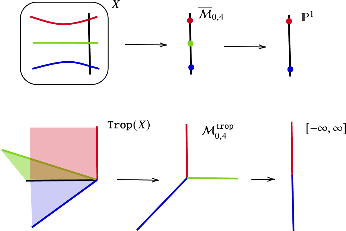

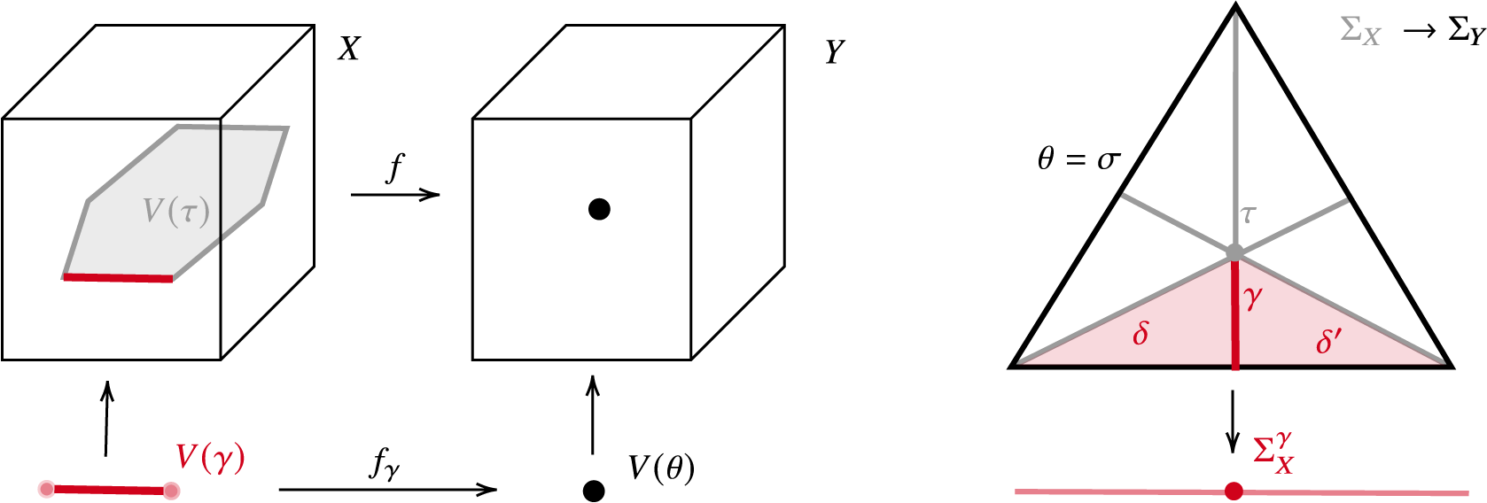


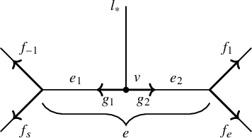

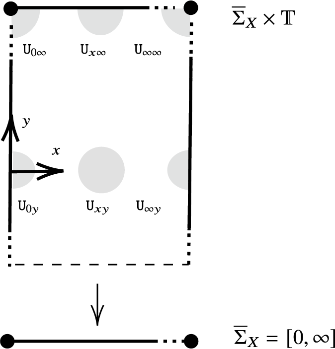


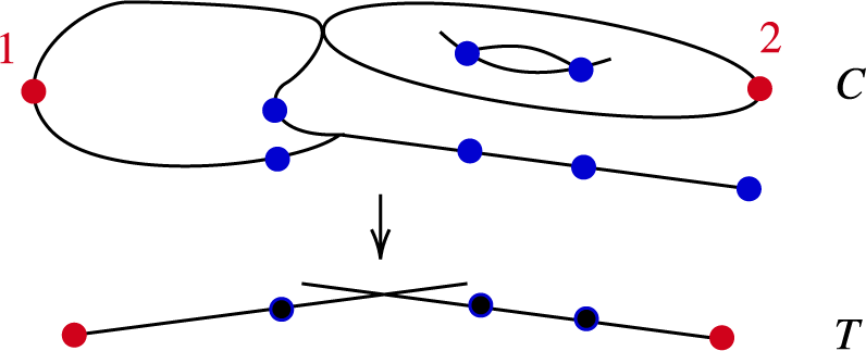


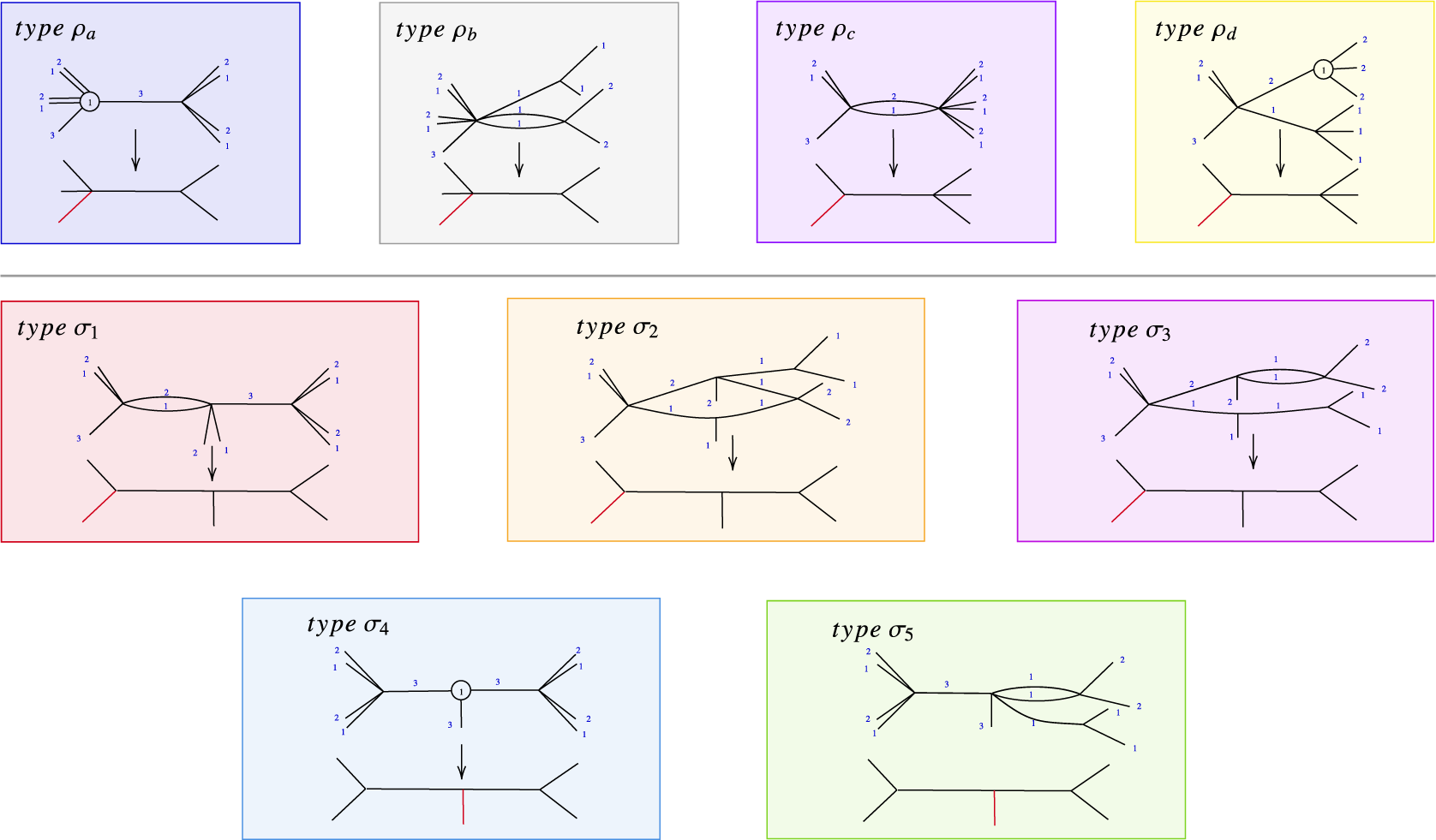


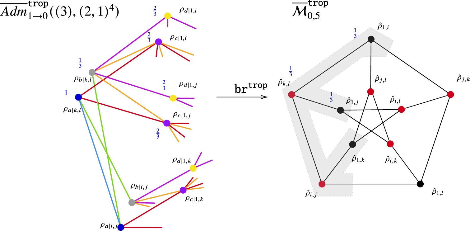


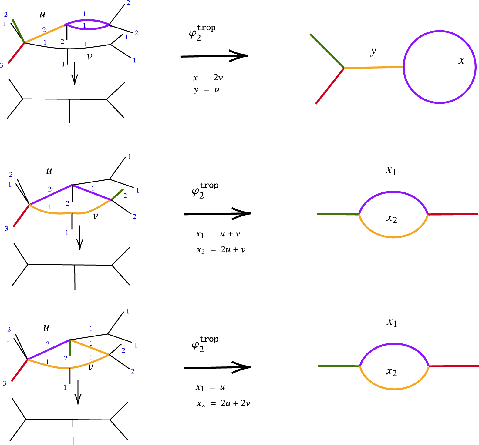


 Open access