





Introduction
As a result of global warming over the last few decades, the Greenland ice sheet has been losing mass at an accelerating rate (Murray and others, Reference Murray2015; Mouginot and others, Reference Mouginot2019), thereby becoming the largest regional contributor to global sea level rise (Bamber and others, Reference Bamber, Oppenheimer, Kopp, Aspinall and Cooke2019; Shepherd and others, Reference Shepherd2020). About half of this mass loss is due to enhanced surface ablation (van den Broeke and others, Reference van den Broeke2016). The other half can be explained by frontal ablation, which is defined as mass loss at the ice–ocean boundary due to a combination of submarine melt and iceberg calving (Fried and others, Reference Fried2019), and related dynamic feedbacks such as retreat, thinning and flow acceleration of ocean-terminating outlet glaciers (Enderlin and others, Reference Enderlin, Howat, Jeong, Noh, van Angelen and van den Broeke2014; Mouginot and others, Reference Mouginot2019; Shepherd and others, Reference Shepherd2020). Observations show substantial mass loss from Greenland’s tidewater glaciers on a large scale across the entire ice sheet margin (Murray and others, Reference Murray2015). Since 2000, notable thinning, together with rapid retreat and acceleration of these tidewater glaciers, has been observed in most regions of Greenland (King and others, Reference King2020). In the South of Greenland, tidewater glaciers are showing particularly high rates of retreat and thinning (Murray and others, Reference Murray2015).
In contrast to the widespread patterns of thinning and retreat observed across most of Greenland, the ocean-terminating outlet glacier Eqalorutsit Kangilliit Sermiat in South Greenland (hereafter EKaS) exhibits very different dynamical behaviour compared to both the ocean- and land-terminating glaciers in Greenland and even to those within the same fjord system. More specifically, EKaS was found to be the only glacier in Greenland with a clearly positive mass change during the period of 1985–2022 (Greene and others, Reference Greene, Gardner, Wood and Cuzzone2024). Furthermore, the EKaS glacier has exhibited terminus advance in recent decades, despite being situated in a region where glaciers generally show pronounced thinning and terminus retreat (King and others, Reference King2020). The identification of the anomalous dynamic behaviour of EKaS is not new. Weidick (Reference Weidick1984, Reference Weidick2009) already documented a continuous advance of the terminus from 1932 to 2006 and produced a map showing the ice margin evolution of EKaS and surrounding glaciers in the 20th century (Fig. 1). The author observed a stagnating advance rate after the turn of the millennium and proposed at the time a stationary or even retreating near future behaviour for EKaS. However, the subsequent two decades have provided no sign of retreat. Furthermore, Weidick mentioned local mass balance conditions due to high precipitation in this region as a potential explanation for the advance but did not further investigate the explanations behind EKaS’s anomalous behaviour.
Map of the ice margin in South Greenland, including EKaS (red rectangle), provided by Weidick (Reference Weidick1984), highlighting the general advance (thin black line) or recession (bold black areas) of the ice margin in the 20th century. Additionally, the filled black areas illustrate the extent of the trimline zone of the historic high-stand, and the dotted line shows the according maximum extent into the fjord of the outlet glaciers. Note that most place names, for example, Narsaq vs Narssaq, use an older spelling convention.

Figure 1 Long description
The map of South Greenland illustrates the ice margin changes during the 20th century. It highlights the Eqalorutsit Kangilliit Sermiat glacier within a red rectangle. The map includes symbols indicating general advance (thin black line) and recession (bold black areas) of the ice margin. The filled black areas represent the extent of the trimline zone of the historic high-stand. A dotted line shows the maximum extent into the fjord of the outlet glaciers. Labeled regions include Eqalorutsit Kangilliit Sermiat, Johan Dahl Land, Narssarssuaq and Narssaq. The map scale is provided at the bottom, ranging from 0 to 20 km. The legend explains the symbols used for advance and recession, as well as the trimline zone extent.
There are several reasons why a glacier can be out of phase with local climatic conditions, such as strongly delayed adjustment due to long response times, surging behaviour, extensive debris cover on the surface or the dynamic feedback related to frontal ablation (Evans and Rea, Reference Evans and Rea1999; Post and others, Reference Post, O’Neel, Motyka and Streveler2011; Rowan and others, Reference Rowan, Egholm, Quincey and Glasser2015; Motyka and others, Reference Motyka2017). The dynamic behaviour of ocean-terminating glaciers is strongly modulated by bed topography, as frontal ablation generally increases with water depth (Pelto and Warren, Reference Pelto and Warren1991; Benn and others, Reference Benn, Warren and Mottram2007). In deep fjords where warm Atlantic water can reach the calving front, the warming of the ocean water drives tidewater glacier retreat and mass loss by enhanced oceanic melt (e.g. Wood and others, Reference Wood2021; Slater and Straneo, Reference Slater and Straneo2022; Brough and others, Reference Brough, Carr, Ross and Lea2023). Additionally, large water depths potentially bring a glacier closer to floatation, where associated stresses lead to larger calving events (e.g. Trevers and others, Reference Trevers, Payne, Cornford and Moon2019; Goliber and Catania, Reference Goliber and Catania2024). Therefore, terminus positions are assumed to be more stable in areas of shallow water depths or constrictions in fjord width (Enderlin and others, Reference Enderlin, Howat and Vieli2013; Vieli, Reference Vieli, Haeberli and Whiteman2015). Consequently, ocean-terminating glaciers can undergo a cyclic pattern that is characterized by a slow terminus advance followed by a fast and unstable retreat (Meier and Post, Reference Meier and Post1987; Pfeffer, Reference Pfeffer2007), even in a stable climate and independently of short-term climatic forcing (Post and others, Reference Post, O’Neel, Motyka and Streveler2011). Within this ‘tidewater glacier cycle’, a glacier starts to advance once the frontal ablation can not keep up with the ice flux supplied to the terminus (Eidam and others, Reference Eidam, Sutherland, Duncan, Kienholz, Amundson and Motyka2020). In a constant climate, the advance requires a reduction in oceanic melt or iceberg calving rates, which is most effectively achieved through the development of a morainal bank by sedimentation and ploughing processes (Post and others, Reference Post, O’Neel, Motyka and Streveler2011; Vieli, Reference Vieli, Haeberli and Whiteman2015). These morainal banks shelter the ice from warm Atlantic sea water, reduce the water depth and thus the calving rates, decrease the buoyancy forces at the ice front and provide additional buttressing (Alley, Reference Alley1991; Post and others, Reference Post, O’Neel, Motyka and Streveler2011). While this process is widely accepted in theory and has been explored in numerical models (Nick and others, Reference Nick, van der Veen and Oerlemans2007; Brinkerhoff and others, Reference Brinkerhoff, Truffer and Aschwanden2017), direct observations thereof are rare. Probably the best-studied examples of the coupling between sedimentation processes and ice front advance are the Hubbard, Yahtse and Taku glaciers in Alaska, whose morainal bank progradation can either be explained by the glacier’s shoving processes (Goff and others, Reference Goff, Lawson, Willems, Davis and Gulick2012), glacio-fluvial erosion and transport of subglacial sediment (Motyka and others, Reference Motyka, Truffer, Kuriger and Bucki2006), or a combination of both.
A few other tidewater glaciers distributed around Greenland also showed a small surface elevation gain at the terminus or a stable to slightly advancing terminus position in recent decades despite a warming climate (e.g. Csatho and others, Reference Csatho2014; Murray and others, Reference Murray2015; Millan and others, Reference Millan, Rignot, Mouginot, Wood, Bjørk and Morlighem2018). However, these changes are often small and within observational uncertainties (Greene and others, Reference Greene, Gardner, Wood and Cuzzone2024). Generally, the glaciers—apart from EKaS—either i) have only a short-term (few years) terminus advance and stabilization in phase with past atmosphere and ocean anomalies (Lea and others, Reference Lea2014; Bunce and others, Reference Bunce, Nienow, Sole, Cowton and Davison2021), ii) have an advancing floating tongue that eventually breaks off in a major calving event (Johannessen and others, Reference Johannessen, Babiker and Miles2013; Hill and others, Reference Hill, Carr and Stokes2017), iii) show clear evidence of surge-type behaviour (Joughin and others, Reference Joughin, Tulaczyk, Fahnestock and Kwok1996; Hill and others, Reference Hill, Carr and Stokes2017), iv) rely on the presence of shallow sills combined with a typical tidewater glacier cyclic retreat and advance (Millan and others, Reference Millan, Rignot, Mouginot, Wood, Bjørk and Morlighem2018), v) have a bed shape that favours the up-glacier propagation of dynamic thickness change (Csatho and others, Reference Csatho2014; Felikson and others, Reference Felikson2017), vi) relate to a region with generally little thinning, terminus retreat or surface velocity change (Walsh and others, Reference Walsh, Howat, Ahn and Enderlin2012; King and others, Reference King2020) or vii) show a much smaller positive net area change and hence advance than EKaS (Kochtitzky and others, Reference Kochtitzky2023). The last point is supported by the findings of Greene and others (Reference Greene, Gardner, Wood and Cuzzone2024), who reported that EKaS is the only glacier with a mass gain that exceeds the measurement uncertainty. Of the explanations listed above, only iii), iv) and v) can not be immediately excluded for EKaS.
Investigating the reasons for the anomalous behaviour of EKaS not only helps us understand the future behaviour of the southern Greenland ice sheet but also broadens our understanding of the processes and interactions at the ice–ocean boundary to inform modelling and related projections of sea-level rise in a changing climate. The aims of this study are, firstly, to systematically document and analyse the anomalous behaviour of EKaS from 1953 to present. This occurs in context of the surrounding glaciers and with regard to surface elevation change, terminus position and ice discharge using remote sensing, in situ hydrography, as well as regional climate data and reanalysis products. In a second step, we analyse potential explanations for the glacier’s anomalous behaviour on the basis of the compiled datasets and supported by ice flow simulations. More specifically, we investigate the following potential explanations:
(1) EKaS is gaining mass because of a
a) current or recent surface mass balance (SMB) surplus as suggested by Weidick (Reference Weidick2009).
b) very long response time and does not yet respond to the climatic warming trend of the recent decades.
(2) EKaS has reduced frontal ablation or shows dynamical thickening caused by
a) reduced water depth and hence reduced calving due to sedimentation processes.
b) a lack of warm Atlantic water.
c) terminus position control on glacier flow and thickness.
d) an already induced advance up a retrograde bed slope.
Data and methods
Study site
The focus of this study is the ocean-terminating glacier EKaS, also locally called Qajuuttap Sermia, located in South Greenland (61.36 $^{\circ}$ N, 45.76 $^{\circ}$ W). This tidewater outlet glacier flows from the ice sheet into the Sermilik fjord, about 27 km north-west of Narsarsuaq (Fig. 2). EKaS drains a basin of roughly 5800 km $^{2}$ (about 0.3 % of the ice-sheet area), encompassing the two basins ‘QAJUUTTAP SERMIA’ and ‘QAJUUTTAP SERMIA N’ defined by Mouginot and Rignot (Reference Mouginot and Rignot2019). Its area corresponds to 83 % of an average Greenlandic tidewater glacier basin size, placing it just outside the top quarter of all ocean-terminating glacier basins in Greenland, while being the largest basin in South Greenland. The basin extends inland to the East–West ice divide. The glacier system of EKaS consists of the main glacier trunk (EKaS) and three north-western tributaries, hereafter EKaST1, EKaST2 and EKaST3, listed in upstream order from west to east (Fig. 2). Currently, these tributaries are rapidly losing mass and no longer contribute to the ice discharge of the main trunk. Therefore, now they can be considered distributaries from the main trunk, as evidenced by the intersecting debris line deposits (e.g. medial moraines), which are increasingly being pushed up into the side valleys (by up to 2 km) by the ice in the main trunk. Large parts of the glacier system are located at a relatively high elevation, with a mean altitude of about 2100 m and an ablation area of only about 10-16 % of the basin (range of past 34 years). The terminus flow speed of EKaS lies between 1.5 km a $^{-1}$ at the end of the melt season and 3.5 km a $^{-1}$ at the beginning of the melt season (Gardner and others, Reference Gardner, Fahnestock and Scambos2023) and shows a strong sensitivity to water input (Dachauer and others, Reference Dachauer, Kneib-Walter, Gräff and Vieli2026). The grounded terminus of EKaS is about 3 km wide and roughly 360 m thick, with about 280 m below the waterline (Rosier, Reference Rosier2025). These dimensions and flow speed produce an annual ice discharge of about 3.1 km $^3$ a $^{-1}$ (Mankoff and others, Reference Mankoff, Solgaard, Colgan, Ahlstrøm, Khan and Fausto2020a).
Overview Sentinel-2 image (2023-07-30) and drainage basin outline (blue line, Mouginot and Rignot (Reference Mouginot and Rignot2019)) of the EKaS glacier system. Additionally, a zoomed-in Sentinel-2 image (top left; 2023-08-07) of the terminus area of EKaS with the three north-western tributaries EKaST1, EKaST2 and EKaST3 (Copernicus Data Space Ecosystem, 2025). The inset map in the top right indicates the location of the study area within Greenland.

Figure 2 Long description
The map shows the Eqalorutsit Kangilliit Sermiat glacier basin outlined in blue, located in South Greenland. The basin is marked with a drainage outline and includes the main glacier trunk and three north-western tributaries labeled as EKaST1, EKaST2 and EKaST3. The inset map in the top right corner indicates the location within Greenland. The map also highlights the proximity to Narsarsuaq, marked in red. The scale bar indicates a distance of 20 km and the map includes elevation contours, with the ice divide labeled. The inset in the top left provides a zoomed view of the terminus area, showing the tributaries in detail. The map uses symbols to denote moraines and sheaths, providing additional geological context.
Data analysis
Terminus positions, climate records and flow speed trends
Building on the work previously conducted by Weidick (Reference Weidick2009), we first updated the existing terminus positions using satellite-derived terminus position products from the past two decades created by MEaSUREs (Joughin and others, Reference Joughin, Moon, Joughin and Black2020) and PROMICE (Andersen and others, Reference Andersen2019), as well as Landsat optical imagery for the terminus position in the 1990s (U.S. Geological Survey, 1999) and Sentinel-2 imagery for the years after 2021 (Copernicus Data Space Ecosystem, 2025). We used a box area approach as described in Black and Joughin (Reference Black and Joughin2022) to consider the variability along the glacier width. Furthermore, we analysed the local climate conditions using temperature records from the Narsarsuaq airport weather station extending back to the 1960s (Drost Jensen, Reference Drost Jensen2023). Finally, we investigated EKaS’s flow velocities using the satellite-derived ITS_LIVE flow speed dataset (Gardner and others, Reference Gardner, Fahnestock and Scambos2023).
Elevation change analysis
To further examine the terminus mass changes of EKaS, we derived maps of surface elevation change using the three digital elevation models (DEMs) ArcticDEM (Porter and others, Reference Porter2022, Reference Porter2023), GIMP DEM (Howat and others, Reference Howat, Negrete and Smith2014) and the AeroDEM (Korsgaard and others, Reference Korsgaard2016). The AeroDEM is derived from Greenland-wide aerial photographs taken in 1985 across South Greenland. Processed using stereo-photogrammetry, it is most reliable along the ice sheet margin, where the image contrast is more pronounced. The DEM has a resolution of 25 m, with external validation indicating an accuracy of 10 m horizontally and 6 m vertically (Korsgaard and others, Reference Korsgaard2016).
The GIMP DEM comes with a spatial resolution of 30 m and represents the surface elevation between the years 2003 and 2009 (nominal date of 2007). The DEM was validated with ICESat, showing an ice-sheet-wide vertical error of 10 m (Howat and others, Reference Howat, Negrete and Smith2014). However, the authors highlight that steep areas in the South of Greenland generally have larger uncertainties, which is relevant for our study area.
Two versions of the ArcticDEM were used in this study. Firstly, for a local and detailed elevation change investigation of the lower 30 km of EKaS with its three north-western tributaries, we used the ArcticDEM strips product (v3.0), which comes with an exact acquisition date taken in the summers of 2012, 2021 and 2024 (Porter and others, Reference Porter2022). Secondly, for a regional-scale elevation change assessment that includes the neighbouring glaciers, the ArcticDEM mosaic (v3.0) was used, which is based on merged photogrammetric elevation models spanning the period 2007–21 (Porter and others, Reference Porter2023). However, for the terminus area of EKaS, the first elevation models are only available from 2012 onward. Assuming a mid-period timestamp (e.g. 2016), the difference between the GIMP DEM and the ArcticDEM mosaic provides a suitable reference to evaluate roughly a decade of elevation change and identify general trends in EKaS compared to adjacent land-based and marine-terminating glacier margins. The ArcticDEM is created using pairs of submeter Maxar satellite images, has a spatial resolution of 2 m for the strips and 10 m for the mosaic, and a vertical uncertainty of less than 1 m on most ice surfaces (Porter and others, Reference Porter2022; Luo and others, Reference Luo, Ke and Fan2024).
All four DEMs were reprojected to WGS 84/NSIDC Sea Ice Polar Stereographic North (EPSG:3413) and further processed using the open-source Python package xDEM (xDEM contributors, 2023). Each DEM was resampled to a 30 m grid using bilinear interpolation. Subsequently, systematic elevation errors in the non-glaciated part of the DEMs need to be corrected (Nuth and Kääb, Reference Nuth and Kääb2011; Hugonnet and others, Reference Hugonnet2022). We applied the following sequential pipeline of three built-in co-registration algorithms in xDEM: vertical shift (vertical translation), ICP (translations and rotations) and Nuth–Kääb (translations), as recommended for DEMs with large vertical differences and rotation (e.g. xDEM contributors, 2023; Zhu and others, Reference Zhu2025). In a last step, the elevation change maps were calculated by subtracting the earlier DEM from the more recent one.
SMB from reanalysis data
Reanalysis data from the two regional climate models MAR and RACMO (e.g.
Shepherd and others, Reference Shepherd2020; Mankoff and others, Reference Mankoff2021; Box and others, Reference Box2022) were used to investigate the influence of a changing SMB on the anomalous behaviour of EKaS. More specifically, we utilized monthly outputs of MAR v3.12 interpolated onto the 1  $\times$ 1 $\text{km}^2$ grid of ISMIP6 using ERA5 (Fettweis and others, Reference Fettweis2017) and yearly data from the Regional Atmospheric Climate Model RACMO2.3p2 at 1 km resolution (statistically downscaled from the output of RACMO2.3p2 at 5.5 km) as detailed by Noël and others (Reference Noël2018). All SMB investigations using modelling data were performed basin-wide and, if not stated otherwise, averaged between 1990 and 2020. In a first step, the SMB from 1990 to 2020 was analysed separately for accumulation (precipitation) and ablation (the sum of evaporation and sublimation for MAR and sublimation for RACMO), and individual trends were calculated. Additionally, continuous operational time series of solid ice discharge (SID) by Mankoff and others (Reference Mankoff, Solgaard, Colgan, Ahlstrøm, Khan and Fausto2020a) were used to set the processes driven by mass balance in the context of total mass balance. The authors calculated the SID for each sector defined by Mouginot and Rignot (Reference Mouginot and Rignot2019) at a gate close to the glacier terminus (approximately 6 km upstream). Thus, the total mass balance (MB) is derived by subtracting the SID at this gate from the balance flux (integrated SMB over the entire basin).
Fjord bathymetry
Existing gridded bathymetric products by IceBridge BedMachine v5 (Morlighem and others, Reference Morlighem, Williams, Rignot and An2022) were combined with several hundred single-point depth soundings from the inner Nordre Sermilik fjord—the inner reach of Ikersuaq Fjord (Figs 1 and 2)—with particularly dense coverage in front of the glacier terminus. These depth sounding data points were collected during three cruises in the summers of 2022, 2023 and 2024 (Rosier, Reference Rosier2025, fig. 12).
Sediment dating
The age of the sediment infill in the fjord at EKaS is estimated from three shell samples in a glaciomarine deposition at the current fjord shore about 2 km east of the calving front (61.31023 N  $-$45.72628 E; Fig. 2). These datings provide a minimum estimate of deglaciation and allow to determine long-term sedimentation rates in front of EKaS. The shell samples have been radiocarbon-dated ( $^{14}$C) at the ETH Zurich AMS facility (Christl and others, Reference Christl2013). The calibration is done using the calib-tool (http://calib.org/calib/) by Stuiver and Braziunas (Reference Stuiver and Braziunas1993) with the Marine20 calibration curve and a marine reservoir correction from the South Greenland average derived by Pearce and others (Reference Pearce, Özdemir, Forchhammer Mathiasen, Detlef and Olsen2023).
Ice flow modelling
Thick, slow-moving inland ice is characterized by delayed responses to external perturbations, often spanning decades to centuries (Wang and others, Reference Wang, Li and Zwally2012). To assess if EKaS’s recent mass gain reflects a lagged reaction to past inland accumulation changes and separately to examine how past terminus position changes at EKaS may have directly influenced its flow dynamics and thickness evolution, we conduct a number of ice flow modelling experiments and estimate the potential drivers, timescales and magnitude of their dynamic response. All simulations are performed using the Ùa community ice flow model (Gudmundsson, Reference Gudmundsson2024), which is initialized by inverting parameters related to basal conditions and ice softness, to match an observed surface flow field. The model domain includes the entire drainage basins of both EKaS and its neighbouring tidewater glacier Eqalorutsit Killiit Sermiat (hereafter EKiS, basin overview Fig. S3), which are exposed to similar atmospheric and oceanic histories. Figure S1 shows the model domain with modelled surface ice speed after initialization (panel a), along with inverted fields for basal slipperiness and ice rate factor (panels b and c, respectively). Also plotted are the two flux gates A–A $^{\prime}$ and B–B $^{\prime}$, at which modelled ice flux and thickness changes are evaluated. Further details of the model set-up are provided in the Appendix. Our model simulations are organized into three sets of experiments: two examining the effects of perturbations in mass balance and one investigating the potential impacts of a prescribed terminus position history.
ELA perturbation experiments ( $\Delta$ELA): The MAR SMB field is uniformly decreased (increased) by 1.0 m a $^{-1}$, effectively moving the equilibrium line altitude (ELA) to higher (lower) elevations and thereby not only reducing (enhancing) accumulation but also increasing (decreasing) ablation.
SMB perturbation experiments ( $\Delta$Acc): Snow accumulation above specific elevation thresholds (1500, 2000 or 2500 m) is halved (doubled), while holding ablation constant.
Advance experiments: Immediately following initialization, the glacier terminus at its present-day position is retreated in a single timestep to the 1953 position as mapped by Weidick (Reference Weidick2009). After a 25 year period with a fixed terminus position, allowing the modelled ice velocity and thickness to adjust to this new configuration, the terminus is continuously advanced, following a similar approach to Bondzio and others (Reference Bondzio2017). The rate of terminus advance is assumed linear between terminus position observations in the years 1953, 1985, 2007 and 2021.
In each experiment, the perturbation is imposed immediately after the initialization procedure in the first timestep of a transient simulation, and we compare the response of the EKaS and EKiS glaciers to each perturbation. In the first two experiments ( $\Delta$ELA and $\Delta$Acc), the SMB field is perturbed over a period of 50 years and then reverted back to the initial values, running the model for a further 450 years. We then analyse the modelled response in ice flux at gates located several kilometres upstream of the termini of the two glaciers (labelled A–A $^{\prime}$ and B–B $^{\prime}$ in Fig. S1). For the $\Delta$ELA and $\Delta$Acc experiments, the position of the calving front is kept fixed at its present-day location (in contrast to the advance experiment). In the advance experiment, the response in ice flux and thickness until the year 2021 was measured. Then, a second reference experiment was conducted that follows the same procedure, but never allows the terminus to re-advance after the 25 year relaxation. Changes in velocity and thickness in the advance experiment are subtracted from changes in the fixed terminus experiment to reveal the model response to terminus advance only.
Results
Anomalous behaviour of EKaS
Climate and terminus advance
In South Greenland, climate conditions have progressively warmed, with yearly temperatures at the Narsarsuaq airport weather station (Drost Jensen, Reference Drost Jensen2023) rising by 1.2 $^{\circ}$ C from 1961 to 2023 (Fig. 3a). In particular, the summer temperatures increased by about 0.25 $^{\circ}$ C per decade (1.5 $^{\circ}$ C from 1961 to 2023) while the winter warming is only about half as pronounced (0.13 $^{\circ}$ C per decade; 0.8 $^{\circ}$ C from 1961 to 2023). In contrast, the ice flow velocity of EKaS, derived from the ITS_LIVE product (Gardner and others, Reference Gardner, Fahnestock and Scambos2023), clearly shows a decelerating trend in all seasons, but less strongly during the summer months June and July (8% reduction) and with higher deceleration rates in the other seasons (20–30% reduction) (Figs 3b and S2d and e). Note, only velocity values since 2014 were used for the trend analysis due to an incomplete dataset in the years before. In parallel, the terminus of EKaS continuously advanced by almost 2 km in the last 70 years (Fig. 3c). The advance rate was highest between 1953 and 1985 (with an average advance rate of 43 m a $^{-1}$), followed by a period of continuous but lower advance rate (15 m a $^{-1}$). In the last decade, the glacier continues to advance, although at a slower rate of a few meters per year, and shows no sign of halt or retreat (Joughin and others, Reference Joughin, Moon, Joughin and Black2020; Copernicus Data Space Ecosystem, 2025). Although the annual advance rate is much smaller than the seasonal terminus position variations of about 100 m (Fig. S2g), the glacier exhibits consistent yearly advancement. The glacier terminus has now advanced to a position where the fjord widens substantially and where the fjord geometry is expected to inhibit further substantial progression of the EKaS terminus (e.g. Enderlin and others, Reference Enderlin, Howat and Vieli2013; Catania and others, Reference Catania2018).
(a) Time series of winter, summer and annual air temperatures at Narsarsuaq airport weather station over recent decades (Drost Jensen, Reference Drost Jensen2023). (b) The satellite-derived ITS_LIVE ice flow velocity of EKaS (in red), featuring emphasized monthly averages for selected months to visualize trends (Gardner and others, Reference Gardner, Fahnestock and Scambos2023). (c) The progression of the EKaS terminus advance (U.S. Geological Survey, 1999; Andersen and others, Reference Andersen2019; Joughin and others, Reference Joughin, Moon, Joughin and Black2020; Copernicus Data Space Ecosystem, 2025).

Figure 3 Long description
The image A showing a line graph with the vertical axis label temperature (degree celsius) and tick labels 10, 0 and minus 10. A legend titled trend (degree celsius slash decade) lists annual (0.20), winter (0.13) and summer (0.25). Three lines run across the plot with dashed trend lines. The image B showing a scatter plot with the vertical axis label velocity (m a superscript minus 1) and tick labels 1000, 2000, 3000 and 4000. A legend titled monthly mean velocity (gradient in m a superscript minus 2) lists March (minus 69), June (minus 28), September (minus 68) and December (minus 82). Many points are plotted across the time axis. The image C showing a line graph with the vertical axis label terminus advance (m) and tick labels 0, 1000 and 2000. The horizontal axis label is time with tick labels 1950, 1960, 1970, 1980, 1990, 2000, 2010 and 2020. A line with circular markers rises from near 0 around the early 1950s to near 1000 around 1980, then to around 1400 in the mid 1980s and continues with smaller step changes to near 2000 by the early 2020s.
The observed climatic signal is also reflected in the SMB. As shown in Fig. 4, the basin-averaged SMB at EKaS has undergone a long-term negative trend of  $-$0.65 mm w.e. a $^{-1}$ from 1840 to 2012 (Box, Reference Box2013). This decline has accelerated markedly over the past three decades ( $-$10 mm w.e. a $^{-1}$) compared to the period before 1990 ( $-$0.14 mm w.e. a $^{-1}$), when the trend was insignificant. To emphasize the anomalous behaviour of EKaS, we compare it to the neighbouring tidewater glacier EKiS. Aside from differences in bed geometry, the two basins share glacier type, climatic conditions (air temperature and precipitation), scale of basin area and SMB. A comparison of bed geometry, ice velocity and terminus position between the three large tidewater glaciers in the region (EKaS, EKiS and Qooqqup Sermia) can be found in the supplementary material, Fig. S2. Additionally, the supplementary material includes a velocity map (Fig. S3) and a 1990–2020 averaged SMB map (Fig. S4), including the basin extents.
EKaS basin averaged SMB from Box (Reference Box2013) for the period 1840–2012, and the regional climate models MAR and RACMO (1990–2020). The numbers represent the SMB trend for each model.

Figure 4 Long description
The graph shows surface mass balance (SMB) trends over time from 1850 to 2012 for Box (2013) and from 1990 to 2020 for MAR and RACMO models. The x-axis represents time in years, ranging from 1850 to 2020. The y-axis represents SMB in millimeters water equivalent per year, ranging from 0 to 1200. Three lines are present: Box (2013) in solid style, MAR in dashed style and RACMO in dotted style. Box (2013) shows a long-term negative trend of negative 0.65 millimeters water equivalent per year, with fluctuations around 800 millimeters. MAR shows a sharper decline of negative 11.6 millimeters water equivalent per year and RACMO shows a decline of negative 9.0 millimeters water equivalent per year. Notable peaks for Box (2013) occur around 1000 millimeters, while MAR and RACMO show more variability with peaks and troughs. The graph highlights differences in SMB trends across models, emphasizing the decline in recent decades.
Visible indicators in the landscape
The anomalous behaviour of EKaS compared to neighbouring glaciers as well as its tributaries is clearly visible in the landscape. The glacier has a convex-shaped surface cross profile all along the glacier tongue (see photograph taken about 1 km upstream from the terminus; Fig. 5a). There, a lateral moraine is actively formed, and fresh vegetation layers have been pushed up the sides. Additionally, along the sides of the main trunk, no vegetation-related trimlines are apparent, indicating that the glacier surface remained stagnant (or even increased) for the last several decades (Fig. 5b). In contrast, a distinct trimline is visible at the same altitude above the EKaST1 tributary, indicating a clear surface lowering over the past 40 years. Already by 1984, Weidick (Reference Weidick1984) published a map of the area around EKaS where advancing and retreating ice margins, as well as trimline zones, were illustrated (Fig. 1). Our observations from today are still in line with this earlier map, namely, the entire ice margin apart from EKaS is receding, and corresponding trimlines are visible.
(a) Actively pushed lateral moraine containing vegetation by a convex-shaped main glacier trunk of EKaS about 1 km upstream from the terminus on the orographic left side in August 2023 (Fig. 2). (b) Visible trimlines on the hillside of the tributary EKaST1 in the far background show a strong surface elevation decrease since the historic high-stand, but no trimlines are apparent at the sidewalls of the main trunk of EKaS. The picture looking into EKaST1 is taken from a similar location as (a) but higher up on the hill. Both images highlight EKaS’s stable, non-retreating behaviour.

Figure 5 Long description
The image A showing a close, oblique photograph along the edge of a glacier. The glacier surface fills much of the frame, with rough ice texture and a steep boundary where ice meets rocky ground. A sloping hillside with rocks and low vegetation runs alongside the glacier margin. Distant mountain slopes and snow-covered areas are present in the background. The image B showing a wide, distant photograph looking across a glacier toward mountain ridges. Text labels above the mountains read no trimline, trimline and no trimline, each with a downward arrow pointing toward the hillside below the label. A horizontal arrow over the glacier is labeled flow direction. Rocky ground with low vegetation occupies the foreground, with the glacier extending across the midground and mountains in the background.
Surface elevation change of EKaS
The thickness change in the ablation area has been estimated by subtracting the surface elevation from two different time steps. Figure 6 shows a regional overview map of the surface elevation change between the ArcticDEM mosaic taken between 2012 and 2021 (Porter and others, Reference Porter2023) and the GIMP DEM from 2003 to 2009 (Howat and others, Reference Howat, Negrete and Smith2014) for EKaS and some of the adjacent land-based and marine-terminating glaciers such as EKiS. Furthermore, Fig. 7 shows a more local and temporally better-resolved elevation difference map between the ArcticDEM strips from 2021 (Porter and others, Reference Porter2022) and the 1985 AeroDEM (Korsgaard and others, Reference Korsgaard2016) for the frontal part of EKaS and its three north-western tributaries. Additionally, the evolution of the terminus as well as of the medial moraines at the intersection between the main trunk and the tributaries is visible for the years of 1953, 1985 and 2021. Both figures, together with Figs 3 and S2f, highlight the strongly contrasting dynamical behaviour of EKaS compared to the ocean- and land-terminating glaciers in the same fjord system. They demonstrate that EKaS has been undergoing continuous and long-term advance, dating back to at least 1953, rather than showing any short-term response to a more recent climatic perturbation. While all adjacent glaciers exhibited surface lowering regardless of their terminus type, the lower part of EKaS (within the ablation area) has been thickening since at least 1985. Frontal thickening at similar magnitudes has been observed attidewater glaciers in Alaska (e.g. Larsen and others, Reference Larsen, Burgess, Arendt, O’Neel, Johnson and Kienholz2015a; Durkin and others, Reference Durkin, Bartholomaus, Willis and Pritchard2017; Berthier and others, Reference Berthier, Larsen, Durkin, Willis and Pritchard2018).
Regional overview of the elevation change map between ArcticDEM mosaic (2012–21) and GIMP DEM (2003–09) over a total period of about 10 years for EKaS and some of the adjacent land-based and marine-terminating glaciers such as EKiS and Qooqqup Sermia. The solid black line represents the 1000 m contour, while the dashed line indicates the 500 m contour.

Figure 6 Long description
The map illustrates elevation change in the EKaS region, focusing on Eqalorutsit Killiit Sermiat (EKiS) and Qooqqup Sermia glaciers. The elevation change is represented by a gradient scale from -40 meters to 40 meters, with blue indicating positive change and red indicating negative change. The solid black line marks the 1000 m contour, while the dashed line indicates the 500 m contour. EKiS is located in the western part of the map, showing areas of elevation decrease. Qooqqup Sermia is situated centrally, also displaying regions of elevation reduction. The map covers a scale of 10 km, providing a detailed view of the glacier dynamics in this area.
Elevation change map between the 2021 ArcticDEM strips and the 1985 AeroDEM of the frontal reaches of EKaS and its three north-western tributaries. The terminus positions and intersecting moraines to the tributaries are shown as coloured lines for the years of 1953, 1985 and 2021.

Figure 7 Long description
The map illustrates elevation change in the EKaS region and its north-western tributaries from 1953 to 2021. Elevation change is represented by a gradient from -100 to 100 meters. The legend indicates changes for the years 2021 (red line), 1985 (blue line) and 1953 (green line). Dashed lines represent transects. EKaST1, EKaST2 and EKaST3 are labeled tributaries. The map shows significant elevation changes, with areas of increase and decrease marked by the color gradient. A scale bar indicates a distance of 5 km.
To analyse the temporal evolution of the surface elevation change at EKaS and its tributaries in more detail, elevation change rate maps of the lower ablation area of EKaS have been created, derived from ArcticDEM strips (2012, 2021 and 2024) and the 1985 AeroDEM (Fig. 8a–c). Figure 8d illustrates the mean surface elevation evolution since 1985 for distinct 1 km $^{2}$ areas of interest (AOIs) at EKaS, EKaST1, EKaST2 and a bedrock reference area. The AOIs of the tributaries are located at an elevation of around 500 m, minimizing the influence of large crevasses due to steep slopes. At EKaS, however, that elevation range and the non-crevassed areas lay outside the ArcticDEM strip margins. Therefore, a central location was selected for both EKaS and the bedrock reference area. EKaS exhibits a total thickening of 18 $\pm$ 4.2 m between 1985 and 2024 at a distance of about 5 km from the terminus, with roughly one-third of the increase occurring after 2021. The thickening rates intensified from 0.3 m a $^{-1}$ during 1985–2012 to 0.4 m a $^{-1}$ in 2012–21, followed by a nearly 7 $\times$ increase to 2.7 m a $^{-1}$ between 2021 and 2024. At the same time, the thinning rate at the tributaries EKaST1 and EKaST2 became increasingly negative, decreasing from $-$1.3 (period 1985–2012) to $-$1.9 m a $^{-1}$ (2021–24) at EKaST1 and from $-$0.8 to $-$1.3 m a $^{-1}$ at EKaST2, respectively. This leads to ice thickness losses over the entire period of $-$57
$-$57  $\pm$ 3.2 m for EKaST1 and $-$38
$-$38  $\pm$ 1.6 m for EKaST2. The reference bedrock area, used for quality control, shows negligible ( $ \lt 1\,\mathrm{m}$) elevation change in all periods. While the elevation change trends are persistent throughout the main trunk of EKaS and its tributaries, the absolute values depend on the location and thus elevation of the selected AOIs. An along-glacier analysis of the surface elevation change can be found in the supplementary material, Fig. S5 for relative and Fig. S6 for absolute values.
(a–c) Surface elevation change rates derived from ArcticDEM strips from 2012, 2021 and 2024 (acquisition date in title in yyyymmdd format), and from the 1985 AeroDEM, shown for the frontal reaches of EKaS and its tributaries EKaST1 and EKaST2. (d) Evolution of mean surface elevation from 1985 to 2024 averaged over 1 km $^{2}$ AOIs at EKaS, EKaST1, EKaST2 and a bedrock reference area (locations indicated by rectangles in panel (a). The numbers along the curves denote elevation change rates between consecutive DEMs. Whiskers indicate the AOI-wide standard deviation of the elevation difference from the earlier DEM.

Figure 8 Long description
The image A showing the title text 20120917 dash 1985. A map with dashed boundary lines and four square markers. A scale bar labeled 3 kilometer and a north arrow are shown. The image B showing the title text 20210907 dash 20120917. A map with dashed boundary lines and four square markers. A scale bar labeled 3 kilometer and a north arrow are shown. The image C showing the title text 20240826 dash 20210907. A map with dashed boundary lines and four square markers. A vertical color scale at the right is labeled elevation change rate (m a superscript negative 1) with tick labels 3, 2, 1, 0, minus 1, minus 2, minus 3. The image D showing a line graph with legend title subset. Legend entries: EKaS, EKaST1, EKaST2, bedrock. The x axis label is time, with tick labels 1985, 1990, 1995, 2000, 2005, 2010, 2015, 2020, 2025. The y axis label is mean AOI DEM evolution since 1985 (m), with tick labels 20, 0, minus 20, minus 40, minus 60. EKaS line: point at 1985 equals 0; point near 2012 is above 0 with an error bar; point near 2021 is above 0 with an error bar; point near 2024 is near 20 with an error bar. Text along the line: 0.3 m a superscript negative 1, 0.4 m a superscript negative 1, 2.7 m a superscript negative 1. EKaST1 line: point at 1985 equals 0; point near 2012 is between minus 20 and minus 40 with an error bar; point near 2021 is between minus 40 and minus 60 with an error bar; point near 2024 is near minus 60 with an error bar. Text along the line: minus 1.3 m a superscript negative 1, minus 1.7 m a superscript negative 1, minus 1.9 m a superscript negative 1. EKaST2 line: point at 1985 equals 0; point near 2012 is between minus 20 and minus 40 with an error bar; point near 2021 is between minus 20 and minus 40 with an error bar; point near 2024 is between minus 20 and minus 40 with an error bar. Text along the line: minus 0.8 m a superscript negative 1, minus 1.3 m a superscript negative 1, minus 1.4 m a superscript negative 1. Bedrock line: point at 1985 equals 0; point near 2012 is near 0 with an error bar; point near 2021 is near 0 with an error bar; point near 2024 is near 0 with an error bar.
Previous studies have observed mass changes at the terminus of EKaS using DEMs (Hugonnet and others, Reference Hugonnet2021; Khan and others, Reference Khan2025). Data from Hugonnet and others (Reference Hugonnet2021) (e.g. the map provided by CNES/CESBIO/IRD/INRAE (2024)) indicate a similar thickening in the ablation area with elevation change rates between 0 and 1 m a $^{-1}$ over the past two decades, while the radar- and altimetry-based DEMs of Khan and others (Reference Khan2022, Reference Khan2025) obscure this anomalous behaviour, likely due to substantial smoothing and interpolation, particularly prevalent in South Greenland. The vertical uncertainty of the DEMs used in our study is below 10 m on ice surfaces, especially near the ice margin (Howat and others, Reference Howat, Negrete and Smith2014; Korsgaard and others, Reference Korsgaard2016; Porter and others, Reference Porter2022, Reference Porter2023). Additionally, the quality of the DEM co-registration was evaluated using the normalized median absolute deviation, which was below 1 m after co-registrations with various versions of the ArcticDEM, approximately 5 m for the AeroDEM, and around 7 m for the GIMP DEM. Thus, the anomalous behaviour of EKaS, with mean AOI surface elevation change of 18 $\pm$ 4.2 m at EKaS and $-$57
$-$57  $\pm$ 3.2 m at EKaST1 for the period 1985–2024, lies beyond any range of error.
Discussion
In the following, we analyse and discuss potential explanations for the observed anomalous dynamics of EKaS, based on the presented data and supported by modelling experiments.
SMB surplus
Accumulation and ablation trends
Weidick (Reference Weidick2009) suggested that large spatial variability in accumulation distribution and corresponding mass balance variations might be responsible for the anomalous behaviour of EKaS. Accordingly, a current or recent positive trend in SMB throughout the drainage basin of EKaS would be the most apparent explanation. We tested this by analysing the modelled 1990–2020 annual SMB both from MAR and RACMO on the EKaS basin and separating it into the components of accumulation and ablation (Fig. 9). In general, the annual accumulation on EKaS decreased in the last 31 years by  $-$5.7 mm w.e. a $^{-1}$ for MAR ( $-$5.1 mm w.e. $^{-1}$ for RACMO), but the trend is not significant ( $p\approx$0.2). At the same time, the ablation is increasing at a similar rate of 5.8 mm w.e. a $^{-1}$ for MAR (4 mm w.e. a $^{-1}$ for RACMO), with $p\approx$0.05. This leads to a significant ( $p \lt 0.05$) overall SMB decrease of $-$11.6 mm w.e. a $^{-1}$ for MAR ( $-$9 mm w.e. a $^{-1}$ for RACMO). The RACMO SMB is slightly more positive compared to MAR, despite the lower accumulation model estimates, mostly due to lower ablation values estimated with RACMO. Longer-term SMB reconstructions between 1840 and 2012 by Box (Reference Box2013) confirm a significant ( $p \lt 0.05$) long-term negative trend ( $-$0.65 mm w.e. a $^{-1}$) in the EKaS basin, with slower rates prior to the past three decades (Fig. 4). Note, for the years 1840–1990, the trend is still negative, but much smaller ( $-$0.14 mm w.e. a $^{-1}$) and insignificant ( $p$=0.6). Spatially, we find no anomalous local SMB pattern that would indicate a more positive SMB in the accumulation area of EKaS compared to the surrounding catchments due to enhanced precipitation from the East (Fig. S4), as proposed by Weidick (Reference Weidick2009). To conclude, the clearly negative trend in accumulation coupled with increasing ablation for both MAR and RACMO indicates opposing long-term tendencies to any large-scale increasingly positive SMB pattern that could support the observed mass gain and terminus advance at EKaS.
Reanalysis based basin averaged SMB (balance fluxes) from the regional climate models MAR and RACMO between 1990 and 2020 on EKaS, separated into their components accumulation (precipitation) and ablation (MAR: melt + evaporation + sublimation, RACMO: melt + sublimation), plotted with the according data trend line and trend rate in mm w.e. a $^{-1}$ (MAR/RACMO) in the legend.

Figure 9 Long description
The graph shows annual mass flux from 1990 to 2020, with the x-axis labeled 'year' and the y-axis labeled 'annual mass flux' in mm w.e. a−1. Three main variables are plotted: accumulation, surface mass balance (SMB) and ablation. Accumulation is represented by blue lines, SMB by green lines and ablation by red lines. Solid lines indicate MAR model data, while dashed lines represent RACMO model data. Each variable has a corresponding linear trend line. Accumulation shows a decreasing trend with peaks around the mid-2000s. SMB fluctuates near zero, with a significant decrease over time. Ablation increases steadily, with notable peaks around 2010. The legend indicates trend rates: accumulation (-5.7/-5.1), SMB (-11.6/-9.0) and ablation (5.8/4.0) in mm w.e. a−1 for MAR/RACMO models. The graph highlights the contrasting trends between accumulation and ablation, contributing to the overall negative SMB trend.
Mass balance comparison with neighbouring EKiS glacier
The SMB of glaciers in the South of Greenland is particularly sensitive to climatic changes (Box and others, Reference Box2022). Accordingly, the surface elevation lowering at the neighbouring glacier EKiS is, together with other land- and ocean-terminating glaciers in the region except EKaS, consistent with the observed negative mass balance trends. Table 1 shows that the two basins have similar mean annual SMBs (period 1990–2020) for both climate models. However, this results in a total mass balance (MB) difference of 0.9 Gt a $^{-1}$ between the two basins after removing the modelled SID (derived by Mankoff and others (Reference Mankoff, Solgaard, Colgan, Ahlstrøm, Khan and Fausto2020a)) at gate 5 km from terminus). While for RACMO this results in a slightly positive total mass balance (MB = SMB $-$ SID) at EKaS and a negative total mass balance for EKiS, for MAR both basins have a negative MB. Interestingly, the annual SMB variability (expressed as the standard deviation throughout the 31 years) is more than $\pm$ 1 Gt a $^{-1}$ for both basins and models. Further, the SID estimates by Mankoff and others (Reference Mankoff, Solgaard, Colgan, Ahlstrøm, Khan and Fausto2020a) are strongly dependent on the poorly constrained bed shape at the flux gate. Therefore, the absolute total mass balance values and their signs should be interpreted with caution, whereas the relative difference between the two basins remains more robust and conclusive.
Elevation and average SMB (1990–2020) statistics for the two main drainage basins, EKaS and EKiS, derived from the regional climate models MAR (Fettweis and others, Reference Fettweis2017) and RACMO (Noël and others, Reference Noël2018). The uncertainty value represents the standard deviation.

Table 1 Long description
The table summarizes elevation, area, and average surface mass balance, ice discharge, and resulting mass balance for two Greenland drainage basins, EKaS and EKiS, using two regional climate models (MAR and RACMO). EKaS has higher mean elevation (2072 m versus 1778 m) and a larger area (5772 square kilometers versus 4399 square kilometers) than EKiS; maximum elevations are 2773 m for EKaS and 2606 m for EKiS. Mean surface mass balance is positive in both basins and is similar across models: about 0.5 to 0.6 m for EKaS and about 0.6 m for EKiS, with uncertainties of roughly 0.2 to 0.3 m. In gigatonnes per year, surface mass balance is higher for EKaS (about 2.7 to 3.3) than for EKiS (about 2.2 to 2.3). Solid ice discharge is about 3.1 gigatonnes per year for EKaS and about 3.5 for EKiS, with smaller uncertainty for EKiS. As a result, mass balance is near zero: EKaS ranges from slightly negative under MAR (about minus 0.4) to slightly positive under RACMO (about plus 0.3), while EKiS is negative under both models (about minus 1.3 to minus 1.2). Uncertainty values are standard deviations, so small differences between models may not be meaningful.
Note: The SID values are obtained from PROMICE (Mankoff and others, Reference Mankoff, Solgaard, Colgan, Ahlstrøm, Khan and Fausto2020a).
The elevation distributions of the EKaS and EKiS basins differ noticeably (Table 1 and Figs S2a–c and S4). EKaS has a higher mean elevation (2072 vs 1778 m) and reaches higher elevations (max. 2773 vs 2606 m), extending up to the main East–West ice divide. Figure 10a indicates the basin areas (solid lines) and mean annual SMB from MAR (1990–2020, dashed lines) in 100 m elevation bands and confirms these findings (Fig. S7 for RACMO). Between 1990 and 2020, the average ELA (where SMB changes sign) was higher for EKaS (1500 m in MAR, 1300 m in RACMO) than for EKiS (1300 m in MAR, 1100 m in RACMO). Thus, about half of EKaS’s surface area lies above 2300 m, which is 800 m above the ELA. In contrast, most of EKiS’s accumulation area lies below 2400 m, with a large proportion being located close to its current ELA. Thus, EKiS may be more sensitive to shifts in ELA (Angelis, 2014). Figure 10b shows the cumulative area from the highest elevation band downward and the corresponding averaged 1990–2020 balance flux, derived by integrating annual SMB over the entire area from the ice divide to the margin. Again, the largest differences between EKaS and EKiS appear around 2000 m for both SMB and balance flux, while the total integrated balance flux at the lowest elevation is similar: EKaS (MAR: 2.7 km $^3$ a $^{-1}$, RACMO: 3.3 km $^3$ a $^{-1}$) and EKiS (MAR: 2.2 km $^3$ a $^{-1}$, RACMO: 2.3 km $^3$ a $^{-1}$). To conclude, although the two basins differ in their area–elevation distributions, this effect is largely mitigated when considering mean SMB values. Furthermore, the total mass balance values come with large uncertainties and similarly sized discrepancies between the MAR and RACMO climate models (Figs 10 and S7), preventing a conclusive interpretation of the contrasting basin behaviours.
(a) Elevation dependency of SMB (from MAR) and area for the two glacier basins EKaS and EKiS in South Greenland. The basins are separated into elevation bands of 100 m, providing the average annual SMB between 1990 and 2020 (dashed lines) and the area (solid lines) for each elevation band. (b) Cumulative area (solid lines) starting from the uppermost elevation band down to the terminus and the averaged 1990–2020 balance flux (dashed lines) from integration of the annual SMB over the area for each band. For analogue results from RACMO, see Fig. S7 in the supplementary material.

Figure 10 Long description
The first graph shows elevation on the vertical axis from 0 to 2500 meters. The horizontal axis shows area in square kilometers from 0 to 1000 and average annual surface mass balance (SMB) from negative 6000 to 2000 millimeter water equivalent per year. Solid lines represent area and dashed lines represent SMB. EKaS and EKiS basins are distinguished by different line styles. EKaS shows higher SMB at elevations above 1500 meters, while EKiS has lower SMB. The second graph shows elevation on the vertical axis from 0 to 2500 meters. The horizontal axis shows cumulative area from 0 to 6000 square kilometers and average balance flux from negative 1 to 4 gigaton per year. Solid lines represent cumulative area and dashed lines represent balance flux. EKaS and EKiS basins are distinguished by different line styles. EKaS shows higher balance flux at elevations above 1500 meters, while EKiS has lower balance flux. Both graphs highlight how SMB and balance flux change with elevation, showing divergence between the basins at higher elevations.
Delayed mass balance response
Thick and slow-moving inland ice masses are known to respond slowly to perturbations, at timescales well beyond a couple of decades or even centuries (Wang and others, Reference Wang, Li and Zwally2012). Thus, we need to consider here if the current mass gain signal of EKaS is not just a strongly delayed response to past inland accumulation perturbations. To test this, we perform simple experiments with the Ùa community ice flow model (Gudmundsson, Reference Gudmundsson2024) for both EKaS and EKiS with step changes to SMB. In a first set of experiments, referred to as  $\Delta$ELA, we uniformly decrease the SMB by 1.0 m a $^{-1}$ throughout the entire domain, thereby not only reducing accumulation but also increasing ablation. In a second set of experiments, referred to as $\Delta$Acc, accumulation in the accumulation zone, above certain elevation thresholds (1500, 2000 and 2500 m), is halved, while holding ablation constant. In both sets of experiments, we reverse the perturbation after a period of 50 years and investigate the response timescales of both glaciers.
Figure 11 shows that the terminus ice flux (solid lines) and ice thickness (dashed lines) response of both glaciers to these two perturbation experiments are quite different. The response of both glaciers to an increase in ELA is an immediate and almost linear decrease in ice flux for the duration of the perturbation, followed by a slow decay, over several centuries, back to the unperturbed state. In contrast, the response to halving of snow accumulation above 2000 m only starts to be felt near the terminus after a delay of several decades, after which ice flux and thickness decrease slowly. This response in ice flux and thickness change peaks well after the perturbation is removed and at different times for the two glaciers (EKaS well before EKiS) and is followed by a slow recovery.
Change in ice flux (solid line) and ice thickness (dashed line) at the termini of EKiS and EKaS for the  $\Delta$ELA (a) and $\Delta$Acc (b) experiments. In $\Delta$ELA, the MAR SMB field is uniformly decreased by 1 m a $^{-1}$ and in $\Delta$Acc, snow accumulation above 2000 m is halved. In both experiments, the perturbation is imposed for 50 years (marked by the dashed line) and then reversed. In panel b, we highlight in red the time period during which the two glaciers show opposing signals to the mass balance perturbation.

Figure 11 Long description
The image A showing Text: Experiment: delta ELA. Legend text: EKaS delta flux; EKiS delta flux; EKaS delta h; EKiS delta h. Horizontal axis label: simulation time (years). Range: 0 to 500. Left vertical axis label: delta ice flux (percent). Range: 0 to negative 40. Right vertical axis label: delta thickness (m). Range: 0 to negative 50. A vertical dashed line is drawn at 50 years. EKaS delta flux (solid line): (0, 0), (50, negative 23), (100, negative 23), (200, negative 16), (300, negative 11), (400, negative 7), (500, negative 5) EKiS delta flux (solid line): (0, 0), (50, negative 32), (100, negative 33), (200, negative 30), (300, negative 26), (400, negative 21), (500, negative 16) EKaS delta h (dashed line): (0, 0), (50, negative 10), (100, negative 10), (200, negative 8), (300, negative 6), (400, negative 4), (500, negative 3) EKiS delta h (dashed line): (0, 0), (50, negative 38), (100, negative 39), (200, negative 33), (300, negative 25), (400, negative 18), (500, negative 12) The image B showing Text: Experiment: delta Acc. Horizontal axis label: simulation time (years). Range: 0 to 550. Left vertical axis label: delta ice flux (percent). Range: 0 to negative 10. Right vertical axis label: delta thickness (m). Range: 0 to negative 8. A vertical dashed line is drawn at 50 years. A shaded vertical band spans from 130 years to 260 years. Legend text: EKaS delta flux; EKiS delta flux; EKaS delta h; EKiS delta h. EKaS delta flux (solid line): (0, 0), (50, negative 3), (100, negative 8), (130, negative 8), (200, negative 7), (260, negative 6), (400, negative 3), (550, negative 2) EKiS delta flux (solid line): (0, 0), (50, negative 1), (100, negative 4), (130, negative 5), (200, negative 6), (260, negative 7), (400, negative 6), (550, negative 5) EKaS delta h (dashed line): (0, 0), (50, negative 2), (100, negative 4), (130, negative 4), (200, negative 3), (260, negative 3), (400, negative 2), (550, negative 1) EKiS delta h (dashed line): (0, 0), (50, negative 1), (100, negative 3), (130, negative 4), (200, negative 6), (260, negative 6), (400, negative 5), (550, negative 4).
One way to characterize the response time of these glaciers to perturbations in SMB is in terms of the e-folding time of their recovery phase. For both experiments, we do a linear regression in log space on the recovery phase of the glacier response to extract the e-folding time. For a uniform 1 m a $^{-1}$ decrease in SMB (experiment $\Delta$ELA), this yields a similar e-folding time of 251 and 244 years for EKaS and EKiS, respectively. For the halving of snow accumulation above 2000 m (experiment $\Delta$Acc), the respective e-folding times are 259 and 413 years for EKaS and EKiS (Fig. 11b), with the ice flux of EKiS only just beginning to slowly recover by the end of the simulation. These experiments were repeated for a change in accumulation at different elevations (1500 and 2500 m) and for an equivalent increase in accumulation (Fig. S8), but in all cases, the e-folding time of EKiS was considerably longer than for EKaS. The reason for the much faster response time of EKaS, despite its larger catchment area, can be explained by its long and narrow outflow channel, resulting in relatively fast flow extending all the way up into the accumulation area ( $ \gt 40\,\mathrm{km}$), whereas at EKiS, high speeds are observed within the first few kilometres ( $ \lt 10\,\mathrm{km}$) of the terminus (Fig. S3). With propagation speed of mass balance or terminus perturbations being proportional to ice speed (Nye, Reference Nye1960), this results in rapid dynamic coupling of the inland ice to the terminus (Felikson and others, Reference Felikson2017).
These modelling results show that the contrasting behaviours between EKiS and EKaS would require a very specific set of circumstances to have arisen as a result of differences in response time to a similar regional perturbation in SMB, namely, for a past negative perturbation in snow accumulation at high altitudes that was later reversed. It is therefore hypothetically possible for EKaS to be in a phase of increasing ice flux and thickening (in response to the reversal of the perturbation) while EKiS is still in a phase of decreasing ice flux and thickness, as a strongly delayed response to said perturbation. In Fig. 11b, we highlight the time window in our  $\Delta$Acc experiment in red, during which the two glaciers exhibit an opposing signal to a past mass balance perturbation. In practice, this explanation relies on our present-day observations falling within a relatively narrow time window after a strong negative accumulation perturbation concentrated at high elevations, followed by a long-term reversal to more positive accumulation. Taken together, the combination of factors needed for this scenario to align with the observations appears unlikely and does not agree with the observed mass balance trends. In contrast, a positiveaccumulation perturbation in the past (i.e. experiment illustrated in Fig. S8) could not produce a state in which EKaS advances while EKiS retreats, since EKaS exhibits a much longer response time independent of the modelled scenario.
Reduced frontal ablation
Since, based on the data and modelling described above, SMB related factors could not explain the anomalous behaviour observed at EKaS, we now investigate whether dynamic feedbacks related to a reduction in frontal ablation (calving and oceanic melt) and basal topography could provide a plausible explanation. The earlier mentioned ‘tidewater glacier cycle’ concept is characterized by a slow advance (time scales of centuries to a millennium), followed by an abrupt and fast retreat phase of decades to a century (Meier and Post, Reference Meier and Post1987; Post and others, Reference Post, O’Neel, Motyka and Streveler2011). It is essentially driven by enhanced frontal ablation in deepening water (Pelto and Warren, Reference Pelto and Warren1991; Benn and others, Reference Benn, Warren and Mottram2007) and hence strongly influenced by the topography of the fjord and glacier bed (Catania and others, Reference Catania2018). The slow and continuous advance of EKaS since at least 1930 would align with the slow advancing phase. This would imply that the evolution of EKaS is largely detached from the climatic forcing, while all surrounding glaciers and tributaries, including other tidewater glaciers such as EKiS and Qooqqup Sermia are strongly thinning in response to the warming climate (Fig. 6). The few other tidewater glaciers that showed terminus advance and dynamical thickening in a negative mass balance regime were found to respond to the development and progradation of a terminal moraine (Durkin and others, Reference Durkin, Bartholomaus, Willis and Pritchard2017). In the following, we discuss factors favouring a dynamical thickening and a slow advance of a tidewater glacier.
To determine the influence of frontal ablation on the anomalous behaviour of EKaS, we briefly discuss the topographic setting and calving style. At EKaS, 280 m of the total ice thickness of 360 m at the terminus lies below the waterline. The terminus is clearly grounded (height above buoyancy at terminus = 57 m, as in Goliber and Catania (Reference Goliber and Catania2024)), which is consistent with the observed lack of tidal impact on the terminus ice flow velocity Dachauer and others (Reference Dachauer, Kneib-Walter, Gräff and Vieli2026). EKaS is therefore classified as a shallow-water grounded calving type (Alley and others, Reference Alley2023) with serac calving as the dominant calving style (Goliber and Catania, Reference Goliber and Catania2024). This calving style implies stronger influence of plume-related submarine melting on calving, and the lack of a floating tongue (even seasonally) points towards a higher sensitivity in terminus dynamics to basal topography (Alley and others, Reference Alley2023; Goliber and Catania, Reference Goliber and Catania2024). The other tidewater glaciers in the region are also above floatation (EKiS height above buoyancy = 16 m, Qooqqup Sermia height above buoyancy = 29 m), but generally closer to floatation than EKaS. While Qooqqup Sermia can also be assigned to a shallow-water grounded calving type, EKiS represents a special case due to its narrow channel (only 1.5 km wide) and steep bed shape towards the terminus (Fig. S2b), and therefore produces strong seasonal variation in terminus position with a short floating tongue in winter (Fig. S2g). In contrast to the relatively shallow and steep adverse bed slopes at the termini of EKiS and Qooqqup Sermia, the calving front of EKaS rests towards the top of a retrograde bed slope, providing a less direct dynamic response to external forcing.
Reduced frontal ablation due to sedimentation
A key factor in the advance phase of the tidewater cycle are sedimentation processes (Pelto and Warren, Reference Pelto and Warren1991; Nick and others, Reference Nick, van der Veen and Oerlemans2007), since calving rates are generally expected to decrease with shallower water depths (Benn and others, Reference Benn, Warren and Mottram2007). In particular, the deposition and reworking of terminal moraines has a large influence on ice dynamics by shielding the glacier from ocean exposure and by providing buttressing and hence reduced ice flux at the terminus that allows a glacier to thicken (Amundson, Reference Amundson2016; Brinkerhoff and others, Reference Brinkerhoff, Truffer and Aschwanden2017). Terminus dynamics and sediment distribution are linked by either large rates of sediment accumulation (sedimentological), fast ice flow leading to the shoving of a terminal moraine (glacigenic), the erosion and redeposition of sediment (glacio-fluvial), or a combination of these processes (e.g. Motyka and others, Reference Motyka, Truffer, Kuriger and Bucki2006; Goff and others, Reference Goff, Lawson, Willems, Davis and Gulick2012). Here we discuss whether any of these sedimentation processes could explain the terminus advance and mass gain of EKaS.
Sediment core analysis by Andresen and others (Reference Andresen2024) from along glacial fjords around Greenland, including Nordre Sermilik at EKaS, found an exponential increase with distance from the major calving termini that were normalized by annual subglacial runoff. When applying the mean annual freshwater discharge at EKaS from 2000 to 2021 of 67–92 m $^3$ s $^{-1}$ (Mankoff and others, Reference Mankoff, Solgaard, Colgan, Ahlstrøm, Khan and Fausto2020a; Hansen and others, Reference Hansen, Karlsson, How, Poulsen, Mortensen and Rysgaard2025) to this relationship, we extrapolate sedimentation rates at the terminus of EKaS to reach 52–71 kg m $^{-2}$ a $^{-1}$, which corresponds to a sediment deposition of 8–27 cm a $^{-1}$ (assuming a water content of 50–80 %). This value is clearly lower than sedimentation rates of about 1 m a $^{-1}$ observed on advancing tidewater glaciers in Alaska (Goff and others, Reference Goff, Lawson, Willems, Davis and Gulick2012) and aligns closely with values reported from other tidewater glaciers in Greenland (Andresen and others, Reference Andresen2024). Over the observed advance phase since the 1950s, such rates would only decrease water depth at the terminus by 6–20 m (2–5 %) and hence are unlikely to suppress calving enough. Note that the relationship by Andresen and others (Reference Andresen2024) is largely unconstrained by sediment core data for distances closer than 5–10 km from the terminus and therefore have large uncertainties. Furthermore, they only consider suspended sediment from subglacial plume discharge (in proximity to calving fronts) and ice-rafted debris from drifting icebergs. Although the inferred average basal erosion rates of 0.38 mm a $^{-1}$ for the combined EKaS and EKiS basins are reasonable (Andresen and others, Reference Andresen2024), these sedimentation estimates do not include local processes at the base of the tidewater glacier ice fronts. Processes such as the shoving of a terminal moraine (glacigenic) or the erosion and transport of subglacial sediment (glacio-fluvial) have been observed to play an important role on tidewater glaciers in Alaska (e.g. Motyka and others, Reference Motyka, Truffer, Kuriger and Bucki2006; Goff and others, Reference Goff, Lawson, Willems, Davis and Gulick2012; Eidam and others, Reference Eidam, Sutherland, Duncan, Kienholz, Amundson and Motyka2020; Zechmann and others, Reference Zechmann, Truffer, Motyka, Amundson and Larsen2021). At EKaS, however, the sea floor is completely flat and smooth, at least up to the surveyed distance of 500 m to the calving front (Rosier, Reference Rosier2025, fig. 12), and shows no signs of a major sediment shoving process. Nevertheless, due to the lack of bathymetric data right at the terminus ( $ \lt 500\,\mathrm{m}$) and given that such a terminus moraine can build up within a few meters of the terminus (Kuriger and others, Reference Kuriger, Truffer, Motyka and Bucki2006), we can not definitely rule out this glacigenic process.
Profile view of EKaS and Sermilik fjord near the terminus. The bed is based on BedMachine v5 (Morlighem and others, Reference Morlighem, Williams, Rignot and An2022), but has been substantially modified over the first 15 km of the transect using our depth-sounding data from the fjord (Rosier, Reference Rosier2025, black line) and by removing clearly erroneous sections beneath the glacier. The ice surface is obtained from the ArcticDEM mosaic (Porter and others, Reference Porter2023).

Figure 12 Long description
Legend: EKaS; Sermilik fjord; modified bed; BedMachine; ELA; depth-sounding. The horizontal axis is labeled transect length from front (kilometer), with labeled ticks at minus 10, 0, 10, 20, 30, 40 and 50. The vertical axis is labeled elevation (meter), with labeled ticks at minus 500, 0, 500, 1000 and 1500. A light-filled area labeled EKaS starts near 0 kilometer at about 100 meters elevation and rises steadily to about 1600 meters by the far right end of the plot. A dark-filled rectangle labeled Sermilik fjord spans from about minus 10 kilometers to 0 kilometer, with its top at 0 meters elevation. A filled area labeled modified bed extends across the full width. From about minus 10 kilometers to 0 kilometer it lies between about minus 450 meters and about minus 300 meters. From 0 to about 10 kilometers it slopes down to about minus 600 meters. Between about 10 and 25 kilometers it stays near minus 600 meters with small undulations. From about 25 to 32 kilometers it rises from about minus 600 meters to about 100 meters. From about 32 to 52 kilometers it rises further to about 1000 meters, then declines slightly to about 850 to 900 meters toward the right edge. A dashed line labeled BedMachine runs close to the modified bed for most of the transect, with a pronounced dip near about minus 2 kilometers reaching roughly minus 700 meters and additional deviations near 0 to 5 kilometers. A dashed horizontal line labeled ELA is drawn at 1500 meters across the plot. A black line with circular markers labeled depth-sounding appears from about minus 10 kilometers to 0 kilometer, with points rising from roughly minus 420 meters to roughly minus 320 meters.
Probably more likely, however, is glacio-fluvial erosion and excavation of soft sediment from beneath the terminal area of the glacier and its immediate redeposition at the terminus. At Taku glacier in Alaska, this process proved to be capable of transporting large amounts of sediment (1–4 m a $^{-1}$ of erosion), despite little evidence of active glacial deformation of a morainal bank (Motyka and others, Reference Motyka, Truffer, Kuriger and Bucki2006; Zechmann and others, Reference Zechmann, Truffer, Motyka, Amundson and Larsen2021). The erosion and transport of sediment largely depends on the water flux and the state of the subglacial drainage system (Swift and others, Reference Swift, Nienow and Hoey2005). EKaS is situated in southern Greenland, and its subglacial freshwater discharge is comparable to that of Alaskan glacial systems (Neal and others, Reference Neal, Hood and Smikrud2010; Mankoff and others, Reference Mankoff, Solgaard, Colgan, Ahlstrøm, Khan and Fausto2020a). The subglacial discharge at EKaS is sediment-rich, which is evident through upwelling plumes near the calving front during the melt season (
Dachauer and others, Reference Dachauer, Kneib-Walter, Gräff and Vieli2026).
$^{-1}$ of erosion), despite little evidence of active glacial deformation of a morainal bank (Motyka and others, Reference Motyka, Truffer, Kuriger and Bucki2006; Zechmann and others, Reference Zechmann, Truffer, Motyka, Amundson and Larsen2021). The erosion and transport of sediment largely depends on the water flux and the state of the subglacial drainage system (Swift and others, Reference Swift, Nienow and Hoey2005). EKaS is situated in southern Greenland, and its subglacial freshwater discharge is comparable to that of Alaskan glacial systems (Neal and others, Reference Neal, Hood and Smikrud2010; Mankoff and others, Reference Mankoff, Solgaard, Colgan, Ahlstrøm, Khan and Fausto2020a). The subglacial discharge at EKaS is sediment-rich, which is evident through upwelling plumes near the calving front during the melt season (
Dachauer and others, Reference Dachauer, Kneib-Walter, Gräff and Vieli2026).
This leads to the question of whether there is enough sediment present below EKaS to allow such a process. The very smooth and flat fjord bed (Rosier, Reference Rosier2025) and unsuccessful core sampling attempts (personal communication, Ian Delaney, July 2022) in front of EKaS demonstrate that the fjord is filled with soft and unconsolidated sediment. The water depth is only gently decreasing from 400 m at a distance of about 10 km away from the terminus towards 280 m at a distance of 500 m from the terminus (Fig. 12). Airborne gravity surveys estimated a bedrock depth (neglecting potential water-saturated sediment layers) in the glacier proximal fjord of EKaS of up to 600 m (Millan and others, Reference Millan, Rignot, Mouginot, Wood, Bjørk and Morlighem2018). This would indicate a thick (200–300 m) sedimentary infill, similar to glacier fjord conditions observed in Alaska (Zechmann and others, Reference Zechmann, Truffer, Motyka, Amundson and Larsen2021). Furthermore, calibrated  $^{14}$C dates of three shell samples from glaciomarine sediments at the shore near the calving front of EKaS (for location see Fig. 2) point towards ice-free conditions since 9.4-9.8 ka BP onwards (Table S1), providing sufficient time for the accumulation of such a thick sediment layer (long-term sedimentation rates of a few centimetres per year).
To conclude, there is no evidence to suggest exceptionally high sedimentation rates at EKaS compared to other tidewater glaciers in Greenland or the shoving of a terminal moraine further than 500 m from the terminus. However, due to the lack of reliable bathymetry data in proximity ( $ \lt 500\,\mathrm{m}$) to the terminus, we can not exclude the build up of such a terminal moraine, or even more likely, the local excavation, transport and deposition of soft sediment from beneath the glacier to the terminus, as observed in similar cases of dynamical thickening at Alaskan tidewater glaciers (Motyka and others, Reference Motyka, Truffer, Kuriger and Bucki2006). If such glacigenic, glacio-fluvial or combined processes are active at EKaS, the advancing glacier would terminate at a moraine bank, which reduces frontal ablation and, importantly, provides additional buttressing, leading to dynamical thickening (Durkin and others, Reference Durkin, Bartholomaus, Willis and Pritchard2017). The available evidence on bathymetry and basal topography shows that we assume that the current advancing terminus sits on a local topographic high (Fig. 12). This topographic setting of the terminus is precisely what would be expected if the glacier were continuously excavating sediment and redepositing it at the terminus (e.g.
Motyka and others, Reference Motyka, Truffer, Kuriger and Bucki2006; Nick and others, Reference Nick, van der Veen and Oerlemans2007; Zechmann and others, Reference Zechmann, Truffer, Motyka, Amundson and Larsen2021).
$ \lt 500\,\mathrm{m}$) to the terminus, we can not exclude the build up of such a terminal moraine, or even more likely, the local excavation, transport and deposition of soft sediment from beneath the glacier to the terminus, as observed in similar cases of dynamical thickening at Alaskan tidewater glaciers (Motyka and others, Reference Motyka, Truffer, Kuriger and Bucki2006). If such glacigenic, glacio-fluvial or combined processes are active at EKaS, the advancing glacier would terminate at a moraine bank, which reduces frontal ablation and, importantly, provides additional buttressing, leading to dynamical thickening (Durkin and others, Reference Durkin, Bartholomaus, Willis and Pritchard2017). The available evidence on bathymetry and basal topography shows that we assume that the current advancing terminus sits on a local topographic high (Fig. 12). This topographic setting of the terminus is precisely what would be expected if the glacier were continuously excavating sediment and redepositing it at the terminus (e.g.
Motyka and others, Reference Motyka, Truffer, Kuriger and Bucki2006; Nick and others, Reference Nick, van der Veen and Oerlemans2007; Zechmann and others, Reference Zechmann, Truffer, Motyka, Amundson and Larsen2021).
Oceanic forcing
A warming of the ocean water column is known to drive retreat and mass loss of tidewater glaciers, in particular in the South of Greenland (e.g.
Wood and others, Reference Wood2021; Slater and Straneo, Reference Slater and Straneo2022; Brough and others, Reference Brough, Carr, Ross and Lea2023). Our newly collected depth sounding data in the inner fjord clearly demonstrate that the fjord is at least 280 m deep until 500 m in front of the terminus of EKaS, and that no shallow sill is present along the fjord towards EKaS (Rosier, Reference Rosier2025). Our CTD casts from several cruises (Fig. S9) and DTS observations from 2023 (Gräff and others, Reference Gräff2025) indicated fjord temperatures of around 3.5 $^{\circ}$ at 260 m depth in front of EKaS and thereby confirm that the warm and saline Atlantic Ocean waters reach all the way to the calving front. Interestingly, at the mouth of the tributary fjord to the neighbouring tidewater glacier EKiS, a clear sill at about 160 m water depth has been observed (Rosier, Reference Rosier2025), which is likely limiting the warm Atlantic Ocean water to access the glacier terminus. At the other large tidewater glacier in the region, Qooqqup Sermia, the sill at the fjord mouth is, with 30 m water depth, even shallower and entirely blocking warm subsurface waters from reaching the calving front (personal communication with Faezeh Nick, Oct. 2024).
Submarine melting is not only influenced by thermal forcing (fjord temperature at depth) but is also amplified by upwelling plumes from subglacial discharge, which is linked to atmospheric warming (Slater and Straneo, Reference Slater and Straneo2022). An increase in submarine melting due to oceanic or atmospheric warming is expected to enhance calving (Alley and others, Reference Alley2023), in particular for relatively shallow-water grounded termini with the dominant calving process of slumping, such as at EKaS, EKiS and Qooqqup Sermia. We estimated rough plume-driven submarine summer melt rates (Fig. S10) using the modelling approach by Slater and Straneo (Reference Slater and Straneo2022), based on thermal forcing data from CTD-casts in summer 2023 located 10–20 km down the fjord (Fig. S9) and subglacial summer discharge (Mankoff and others, Reference Mankoff2020b). The obtained submarine melt rates for EKaS, ranging from 3.5 to 4.1 m d $^{-1}$ (Fig. S10), are 3–10 times higher than those observed on EKiS and Qooqqup Sermia, leading to the highest melt-to-velocity ratio of all three glaciers.
Thus, any warming of both the Atlantic Ocean water or the atmosphere, as observed over several recent decades (Straneo and Heimbach, Reference Straneo and Heimbach2013; Slater and Straneo, Reference Slater and Straneo2022) should impact frontal ablation more strongly at EKaS than at EKiS or Qooqqup Sermia, respectively. The reduced sensitivity of EKiS and Qooqqup Sermia to oceanic forcing together with their clear trend of thinning and retreat implies that their evolution is dominated by the long-term negative SMB and hence the related reduction in ice-delivery to the terminus. As discussed above, the potential presence of a terminal moraine (lack of bed data within  $ \lt 500\,\mathrm{m}$ to the terminus) at EKaS could still limit oceanic melt or at least reduce the relative impact of oceanic forcing on frontal ablation. Since this would only impact the frontal ablation at the few lowest tens of meters of EKaS’s terminus, we expect no substantial change in overall frontal ablation. It is important to note here that the terminus of EKaS in itscurrent stabilizing topographic configuration (width and retrograde slope) and advancing trajectory seems to be relatively insensitive to enhanced frontal ablation. To conclude, based on these considerations and our presented evidence, we do not consider oceanic forcing to be a likely major driver of EKaS’s anomalous behaviour.
Response to changes in terminus position
To investigate how historical variations in the EKaS terminus position may have directly contributed to dynamic changes in glacier flow and thickness, we run a third set of modelling experiments, referred to as the advance experiment. After initialization, the terminus is instantly shifted to its 1953 position and held fixed for 25 years to allow dynamic adjustment. The model then advances the terminus continuously through the observed 1985, 2007 and 2021 positions, and we simulate EKaS’s response in ice flux and thickness until the year 2021. As a reference, a second experiment repeats this procedure but never allows the terminus to re-advance after the 25 year relaxation. All of these model experiments use the same SMB forcing as the mass balance experiments (see Appendix). Modelled ice flux and thickness changes for the reference experiment are shown in Fig. S11. Velocity and thickness changes from the advance experiment are then subtracted against this fixed-terminus reference experiment to reveal the model response to terminus advance only.
We show this relative change in ice flux and ice thickness at a gate just upstream of the 1953 terminus position in Fig. 13. In response to a steady and continuously advancing terminus position, EKaS shows a relatively slow thickening and decrease in velocity until the mid-2000s, at which point thickening accelerates and velocity decreases substantially, leading to an overall decrease in ice flux. During the course of the advance experiment, ice flux near the terminus approximately halves, and average ice thickness across the gate increases by  $\sim$30 %. Between 1985 and 2021, ice thickness increases by almost 100 m near the terminus, which is substantially more than the observed thickening shown in Fig. 7. Although the fixed-terminus reference simulation is not in steady-state and continues to thin slowly after the 25 year relaxation (Fig. S11), this residual drift is much smaller than and opposite in sign to the strong dynamical thickening and slowdown in the advance experiment, suggesting that the experiment is a conservative estimate of terminus-advance-driven thickening and slowdown.
Time series showing change in terminus advance rate (a), ice flux (b) and change in ice thickness (c) at the flux gate just upstream of the 1953 terminus for the advance experiment (prescribed terminus position advance), compared to a model simulation with a terminus fixed at the 1953 position. Model quantities for calculations of flux and thickness are extracted and averaged along a gate  $\sim$1 km upstream of the 1953 terminus position. Dashed lines show times when the terminus position is constrained by observations.

Figure 13 Long description
The image A showing a line graph labeled a. Horizontal axis label: year. Range: 1950 to 2020. Vertical axis label: terminus advance rate (m/yr). Range: 10 to 30. A step line is shown. It is at 30 from 1950 to 1985, at 20 from 1985 to 2007 and at 30 from 2007 to 2020. The image B showing a line graph labeled b. Horizontal axis label: year. Range: 1950 to 2020. Vertical axis label: change in ice flux (Gt/yr). Range: 0 to negative 1. A line starts near 0 around 1953, then decreases to about negative 0.2 by the late 1950s. It fluctuates around negative 0.2 to negative 0.3 through the 1960s and 1970s. It is around negative 0.35 near 1980. From about 1985 to about 2000 it stays near negative 0.3. Around 2002 it drops to about negative 0.45, then rises slightly to about negative 0.4 by about 2006. Around 2007 it drops to about negative 0.6 and stays near negative 0.6 to negative 0.7 through about 2012. Around 2013 it drops to about negative 1.1, then reaches about negative 1.3 by about 2015. From about 2016 to 2020 it stays near negative 1.3. The image C showing a line graph labeled c. Horizontal axis label: year. Range: 1950 to 2020. Vertical axis label: change in ice thickness (m). Range: 0 to 150. A line starts near 0 around 1953. It rises to about 20 by about 1960, about 30 by about 1965, about 35 by about 1970, about 45 by about 1980 and about 50 by about 1985. It rises to about 55 by about 1990 and about 60 by about 2000. It rises to about 70 by about 2005, about 80 by about 2010 and about 95 by about 2014. It rises to about 120 by about 2017 and reaches about 150 by about 2020.
The slowing and thickening response is relatively confined to the first 20–25 km upstream of the terminus and decays in an upstream direction (Fig. S12), indicating that the thickening originates from changes at the terminus. Our advance experiment shows that advance of the terminus between 1953 and 2021, and in particular in the recent past, into shallower water depths would lead to substantial deceleration and dynamical thickening of the lower elevation portion of EKaS, qualitatively mirroring the observed spatial patterns of EKaS and other tidewater glaciers (Durkin and others, Reference Durkin, Bartholomaus, Willis and Pritchard2017; Berthier and others, Reference Berthier, Larsen, Durkin, Willis and Pritchard2018). Uncertainty in bed topography directly upstream of the terminus means that these results are very tentative, but they indicate it is possible that an advance over an upward sloping bed, combined with increased lateral drag from the glacier sidewalls, may explain some of the observed changes on EKaS. Our approach can not directly attribute this change in terminus position to any internal or external driver, but it indicates that the overall thickening response is likely a result of a complex interplay between changes in calving, bed topography and ice dynamics.
Reduced frontal ablation due to retrograde bed slope
The behaviour of tidewater glaciers can differ markedly, even among neighbouring systems exposed to similar atmospheric and oceanic conditions (e.g. Csatho and others, Reference Csatho2014; Bartholomaus and others, 2016; Carr and others, Reference Carr, Stokes and Vieli2017), likely because the bed shape exerts a strong control on the retreat behaviour of tidewater glaciers (e.g. Vieli and others, Reference Vieli, Funk and Blatter2001; Enderlin and others, Reference Enderlin, Howat and Vieli2013; Catania and others, Reference Catania2018). Our knowledge about the bed topography proximal to the calving front (within 500 m of the terminus), and in particular below the terminus area of EKaS, is relatively poor. Here, bed topography datasets such as BedMachine (Morlighem and others, Reference Morlighem, Williams, Rignot and An2022) rely primarily on mass conservation assumptions. The data is particularly poorly constrained near calving termini, where deep and heavily crevassed ice limits the quality of radio-echo sounding (Morlighem and others, Reference Morlighem2017). The bed from BedMachine v5 (Morlighem and others, Reference Morlighem, Williams, Rignot and An2022) dataset is clearly inconsistent with our in situ fjord depth measurements and, therefore, needs to be modified for our model domain (Figs 12 and S2a–c). Millan and others (Reference Millan, Rignot, Mouginot, Wood, Bjørk and Morlighem2018) used a gravity inversion approach to better constrain the bed topography of several glaciers in South Greenland, including EKaS, and found a retrograde bed slope for the first 20 km upstream of EKaS’s terminus, which is used for the bed modification.
The terminus advance experiment (described above) found that any advance would, due to a shallowing of the bed, substantially reduce the terminus ice flux and flow and produce mass gain and dynamical thickening from the terminus upstream but above observed magnitudes. This indicates that any small advance of the terminus on this retrograde slope, for whatever reason, would likely lead to a self-sustained advance and thickening of the terminus (Nick and others, Reference Nick, van der Veen and Oerlemans2007), potentially, even under a warming and negative SMB scenario (although somewhat subdued). The observed decaying thickening pattern from the terminus upstream is also consistent with the mass change originating from advance of the terminus (Nick and others, Reference Nick, Vieli, Howat and Joughin2009).
The questions remain of why EKaS in the 1950s was in a transient state of advance and why the terminus was much more retreated than today. However, there is evidence indicating that the ice sheet margin in South Greenland was retreated behind its current position until 1 ka (Larsen and others, Reference Larsen2015b; Luetzenburg and others, Reference Luetzenburg2026), potentially even as recently as 500 years ago (Young and Briner, Reference Young and Briner2015). Given our analysis so far, we can not rule out that EKaS has been in the latter stage of a transient advance phase in the last few decades (shallowing bed) as part of a longer-term tidewater cycle and that its behaviour is strongly influenced by the geometric configuration of the glacier and fjord.
Other potential influences
EKaS has so far not been identified as a surge-type glacier (e.g.
Weidick and others, Reference Weidick, Ce and Knudsen1992; Kääb and others, Reference Kääb, Bazilova, Leclercq, Mannerfelt and Strozzi2023; Lovell and others, Reference Lovell2023; Guillet and others, Reference Guillet, Benn, King, Shean, Mannerfelt and Hugonnet2025). Aside from its terminus advance, it exhibits no evidence of the characteristic features of surge-type behaviour—such as large periodic changes in flow velocity or glaciological/geomorphological indicators of flow oscillation (e.g. looped moraines) (Sevestre and Benn, Reference Sevestre and Benn2015; Lovell and others, Reference Lovell2026). Most marine-terminating glaciers that have experienced surging are located in western and eastern Greenland. South Greenland generally exhibits low surge potential (Lovell and others, Reference Lovell2026), hosting only a few ( $n$ = 7) known surge-type glaciers, the majority of which ( $n$ = 5) are marine-terminating (Lovell and others, Reference Lovell2023). From these glaciers, however, only one relatively small glacier has been observed to actively surge in the last decades, whereas the others have surged in the past centuries (Lovell and others, Reference Lovell2023). For these reasons, we consider a surge unlikely to explain EKaS’s anomalous behaviour, although a unique and very slow surge at century timescales can not be entirely ruled out.
A unique basal sliding behaviour of the glacier—for instance, triggered by subglacial lake drainage events—cannot also be ruled out. At EKaS, such lake drainage events are known to occur periodically from the tributary EKaST1, typically 1–2 times each summer. This can temporarily influence flow velocities ( Dachauer and others, Reference Dachauer, Kneib-Walter, Gräff and Vieli2026) and potentially change the basal conditions. Unique, periodic elevation change linked to proglacial lake discharge events has previously been observed at Daugaard-Jensen Glacier (Csatho and others, Reference Csatho2014), but has at EKaS so far not been detected.
Conclusions
The ocean-terminating outlet glacier EKaS in South Greenland exhibits markedly different dynamical behaviour compared to both ocean- and land-terminating glaciers in Greenland, even those within the same fjord system. It is the only glacier in Greenland observed to have a mass gain exceeding the measurement uncertainty (Greene and others, Reference Greene, Gardner, Wood and Cuzzone2024). In contrast to the widespread thinning and terminus retreat under the current atmospheric and oceanic warming around Greenland, the main trunk of EKaS has continued to thicken—and is doing so at an increasing rate—while advancing over the recent few decades. Its terminus advanced by nearly two kilometres over the past 70 years, and a thickening by 18 m was observed between 1985 and 2024 (one-third of which occurred within the past 3 years) at a representative area 5 km from the terminus. Lateral moraines containing vegetation, which are actively pushed aside, and absent trimlines provide visible evidence in the landscape. Although the growth of this glacier has already been reported by Weidick (Reference Weidick2009), we document its continuing and recently even intensifying trend up to the present. Furthermore, we have explored various potential explanations of EKaS’s anomalous behaviour, focusing on SMB and reduced frontal ablation. Our analysis integrates available data, reanalysis results and glacier model experiments.
SMB data from the MAR and RACMO reanalysis models indicate increasingly negative accumulation trends and enhanced ablation since 1990, ruling out a potential sustained positive SMB as the driver of the observed long-term thickening at the terminus of EKaS. This negative SMB trend persists even though EKaS has a high average elevation (2072 m) compared to neighbouring glaciers, with a large fraction of its basin area lying well ( $ \gt 800\,\mathrm{m}$) above the ELA. Ice flow model experiments were conducted to test whether EKaS’s behaviour may reflect a delayed positive mass balance signal from the longer-term past. However, in all simulations, EKaS shows a faster response time than its strongly thinning and retreating neighbouring glacier EKiS. In fact, reproducing retreating and thinning EKiS alongside advancing EKaS requires a highly unlikely combination of factors, rendering delayed response time an unlikely explanation for EKaS’s terminus thickening and advance.
Reduced frontal ablation due to oceanic forcing can also largely be excluded, since the 280 m deep ice front at EKaS is much more exposed to the observed increasing trend of the warm Atlantic waters, compared to the two neighbouring tidewater glaciers that are shielded by shallow sills but rapidly thinning. Sedimentation and the build-up of a morainal bank at the glacier terminus could potentially reduce the frontal ablation or provide additional buttressing, thereby leading to an advance. While unrealistically high sedimentation rates would be required, intense shoving of a morainal bank or sediment erosion and redeposition are more likely to have produced such an effect at EKaS. However, our bathymetric observations, unfortunately limited to beyond 500 m from the terminus, provide no direct evidence for these processes.
Ice flow model simulations prescribing observed glacier advance since 1953 qualitatively reproduced the observed thickening pattern. Advancing the terminus over this shallowing bed leads to reduced water depth at the calving front, thereby causing localized thickening and flow deceleration within the lowermost 25 km of the glacier. This dynamical thickening and slowdown response suggests that even modest terminus advances could trigger a self-sustained advance, potentially persisting under warming and negative SMB conditions. A potential morainal bank at the terminus might further amplify such a dynamic advance through additional buttressing and reduced frontal ablation. EKaS could therefore be in the late advance phase of a longer-term ‘tidewater cycle’, which is strongly influenced by the shape of the glacier and fjord bed, although the reason for its retreated position in the 1950s remains unresolved. The basin’s elevation–area distribution, which suggests a relatively low sensitivity to current changes in ELA, together with its generally less negative total mass balance compared to neighbouring glaciers, may favour such a configuration. While uncertainties in bed topography limit confidence, our results point to a complex interaction between bed shape, calving dynamics and ice flow as key contributors to the observed anomalous behaviour.
Supplementary material.
The supplementary material for this article can be found at https://doi.org/10.1017/jog.2026.10172.
Acknowledgements
We are grateful to Dominik Gräff, Manuela Köpfli and Diego Wasser for their field support during the collection of CTD-casts in summer 2023. Further, we acknowledge the reviews by Jason Amundson and an anonymous reviewer, which significantly improved the manuscript. This study is part of the SPI flagship initiative GreenFjord, funded by the Swiss Polar Institute (project number SPI-FLAG-2021-002).
Appendix: Detailed methods of ice flow modelling
We conduct a number of ice flow modelling experiments to better understand possible drivers and timescales of change of the EKaS glacier. All simulations use the Ùa community ice flow model (Gudmundsson, Reference Gudmundsson2024) which uses the shallow ice stream approximation (SSTREAM or SSA; Hutter (Reference Hutter1983); MacAyeal (Reference MacAyeal1989)) to solve for ice flow, using the finite element method on an irregular triangular mesh (with a variable element size from  $\sim$1500 to $\sim$120 m, refined in areas of fast flow and high strain rates). The model is initialized using a control method approach, whereby the spatial distribution of ice rate factor $A$ and basal slipperiness $C$ are optimized via inverse methods using measurements of ice velocity, thickness and thinning rates. The Glen-Steinemann flow law determines the relationship between strain rates $\dot{\varepsilon}$ and deviatoric stresses $\tau$:
 \begin{equation}
\dot{\varepsilon} = A\tau_E^{n-1}\tau
\end{equation}
\begin{equation}
\dot{\varepsilon} = A\tau_E^{n-1}\tau
\end{equation}where  $n=3$ in all experiments. Basal sliding is modelled using a mixed Coulomb–Weertman sliding law:
 \begin{equation}
\boldsymbol{t}_b=\frac{\mu_kN}{\mu_kN+\beta^2\left \| \boldsymbol{v}_b \right \|} \, \beta^2\, \boldsymbol{v}_b \; ,
\end{equation}
\begin{equation}
\boldsymbol{t}_b=\frac{\mu_kN}{\mu_kN+\beta^2\left \| \boldsymbol{v}_b \right \|} \, \beta^2\, \boldsymbol{v}_b \; ,
\end{equation}where  $\beta^2 = C^{-1/m}\left \| \boldsymbol{v}_b \right \|^{1/m-1}$, $N$ is the effective pressure, $\mu_k$ is the coefficient of friction, and generally $m=3$ in all model experiments unless stated otherwise. For the purpose of calculating $N$, we assume perfect hydraulic conductivity of the glacier with the ocean, meaning we assume the basal water pressure beneath the glacier is equal to the water pressure exerted by the sea level at the glacier terminus.
The model inversion minimizes the misfit between observed surface ice velocities and surface elevation change and includes regularization to ensure well-posedness. Four regularization parameters penalize deviation in the  $A$ and $C$ fields from their priors, and penalize less smooth solutions. These four parameters are selected via a standard L-curve analysis approach. The prior for $C$ is based on a rough estimate of basal shear stress, that is, $\tau _b = \rho _i gH\text{sin}(\alpha)$, together with satellite measurements of surface speed and under the assumption of a Weertman basal sliding law. The prior for $A$ is a spatially uniform value equivalent to a depth-averaged ice temperature of 10 $^\circ $C.
In order to reduce shocks (large adjustments) in the transient solution that occur immediately after initialization, largely as a result in poor knowledge of the bed shape, the model undergoes a 2 year transient relaxation period after a first inversion, followed by a second inversion using the relaxed surface geometry at the end of the 2 years. This relaxation of the surface, commonly used in ice sheet models of this type (Goelzer and others, Reference Goelzer2018), greatly reduces the otherwise large rates of surface elevation change that occur across fast-moving portions of the glacier.
The model is nominally initialized for the year 2021, and we use the MEaSUREs version 4 annual Greenland velocity product that covers the period 1st December 2020 to 30th November 2021 for this purpose (Joughin and others, Reference Joughin, Moon, Joughin and Black2020). Ice sheet geometry is from BedMachine v5 (Morlighem and others, Reference Morlighem, Williams, Rignot and An2022), whose end date is set as 31st December 2021. The model domain boundary is selected to lie approximately along ice divides or ice-free areas, allowing for a Dirichlet boundary condition at these boundary nodes, whereby the two horizontal velocity components  $u_b$ and $v_b$ are there set to zero. Close to the glacier terminus, where BedMachine interpolates highly uncertain bed shape from beneath the glacier with the previously unknown fjord shape, artefacts are clearly visible in the BedMachine product, resulting in non-physical step-changes in the bed. Within this limited region, we replace the BedMachine bedrock elevation with our own product (Fig. 12), making use of new measurements of fjord bathymetry taken close to the glacier terminus (Rosier, Reference Rosier2025) and the information of airborne gravity surveys (Millan and others, Reference Millan, Rignot, Mouginot, Wood, Bjørk and Morlighem2018). A smooth transition is enforced between the BedMachine bedrock and our own product by adding BedMachine data close to the boundary of our Kriging region. Within this limited region, we retain the BedMachine surface elevation and ice thickness is therefore adjusted to be consistent with our new bedrock shape. All model experiments use the same reference SMB field, derived by temporally averaging SMB from the MAR reanalysis model for the year 2021 (Fettweis and others, Reference Fettweis2017).

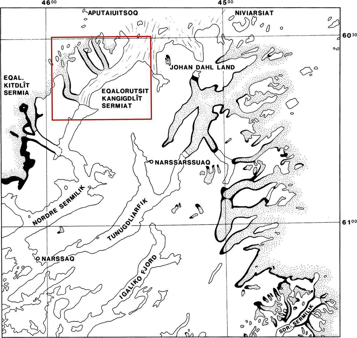
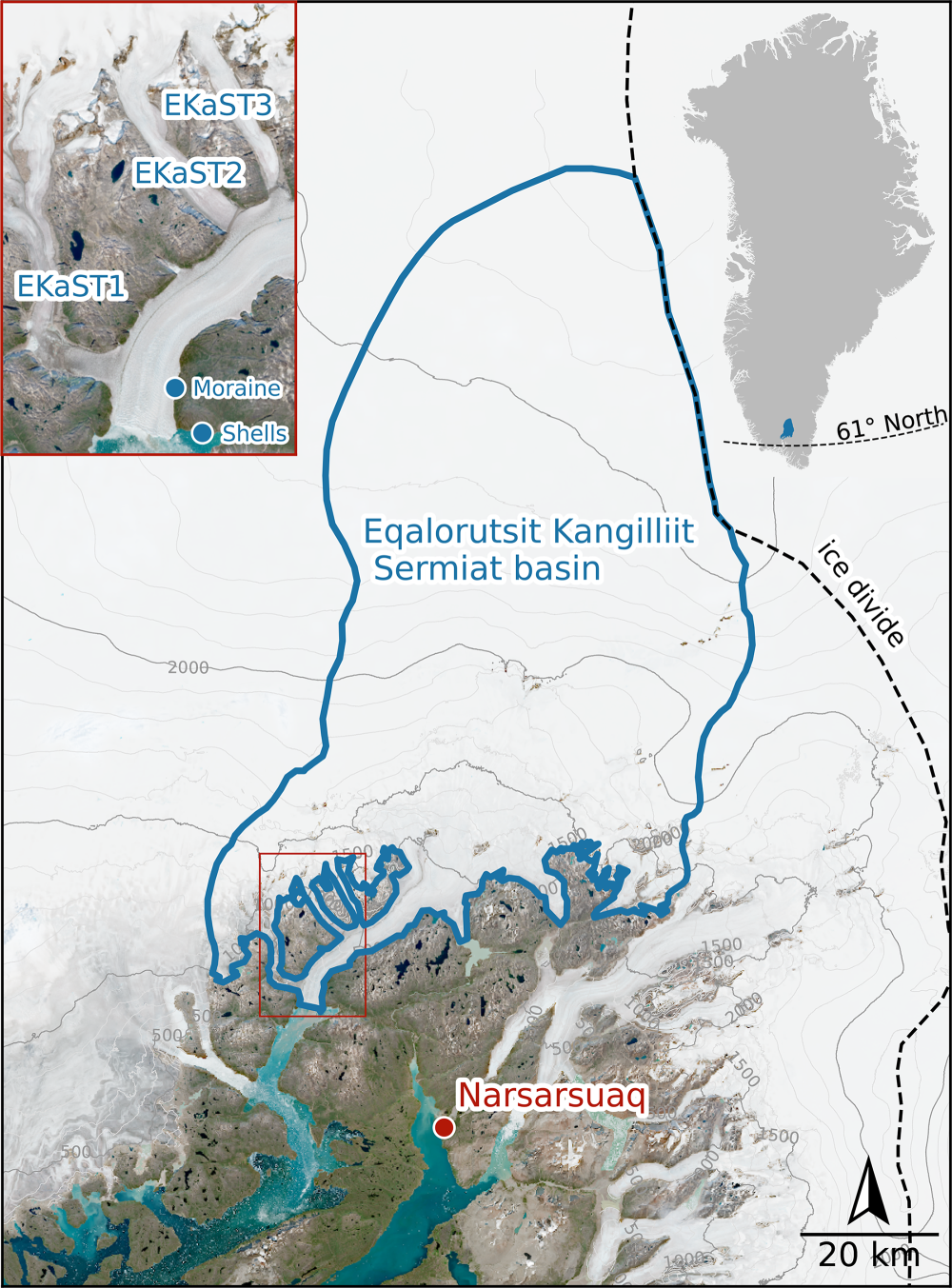
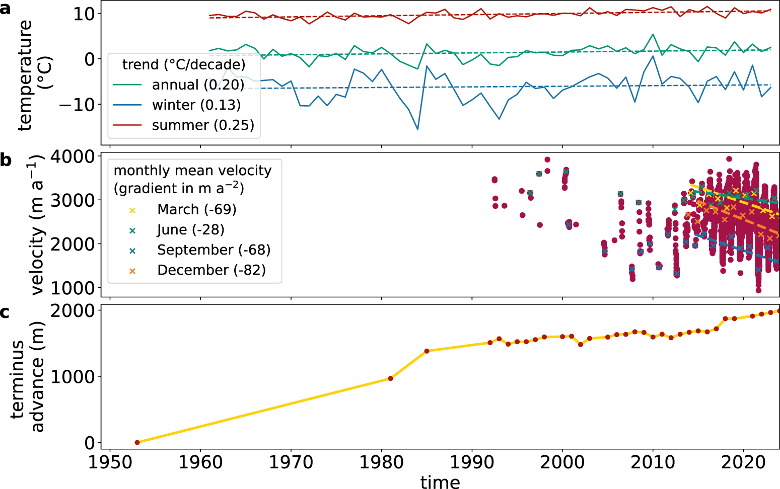
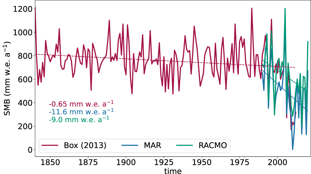
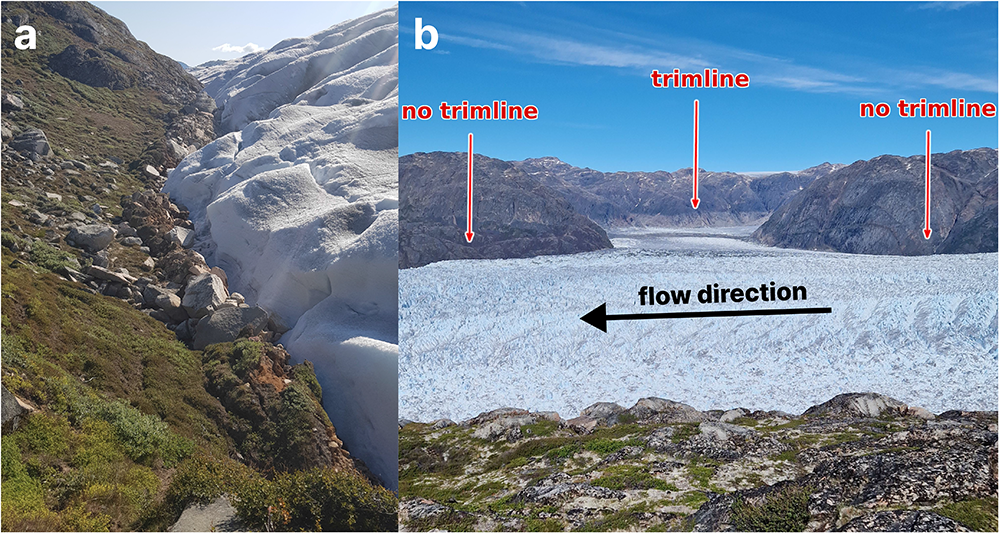
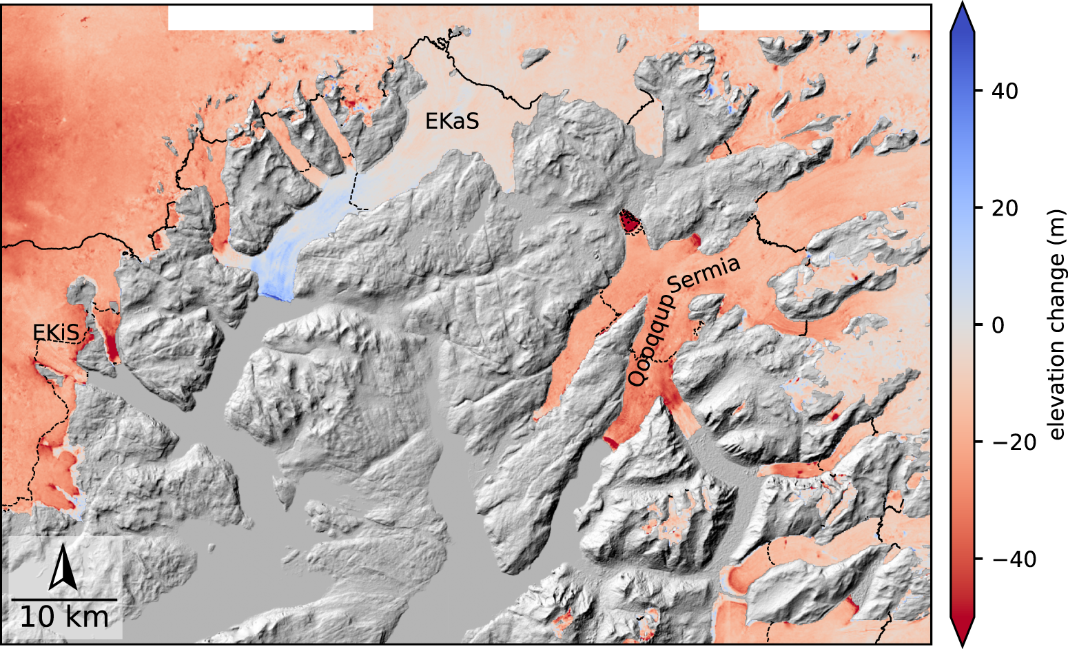
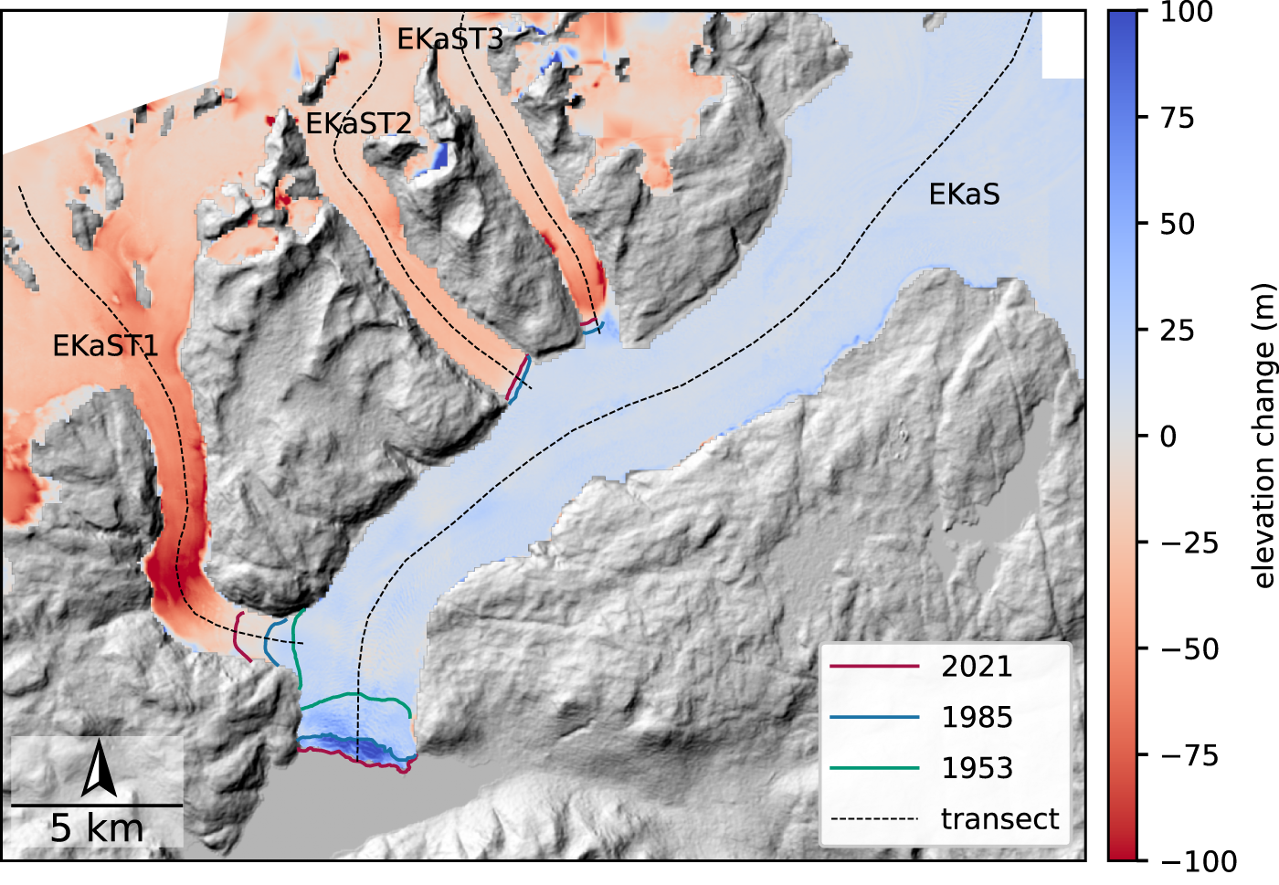
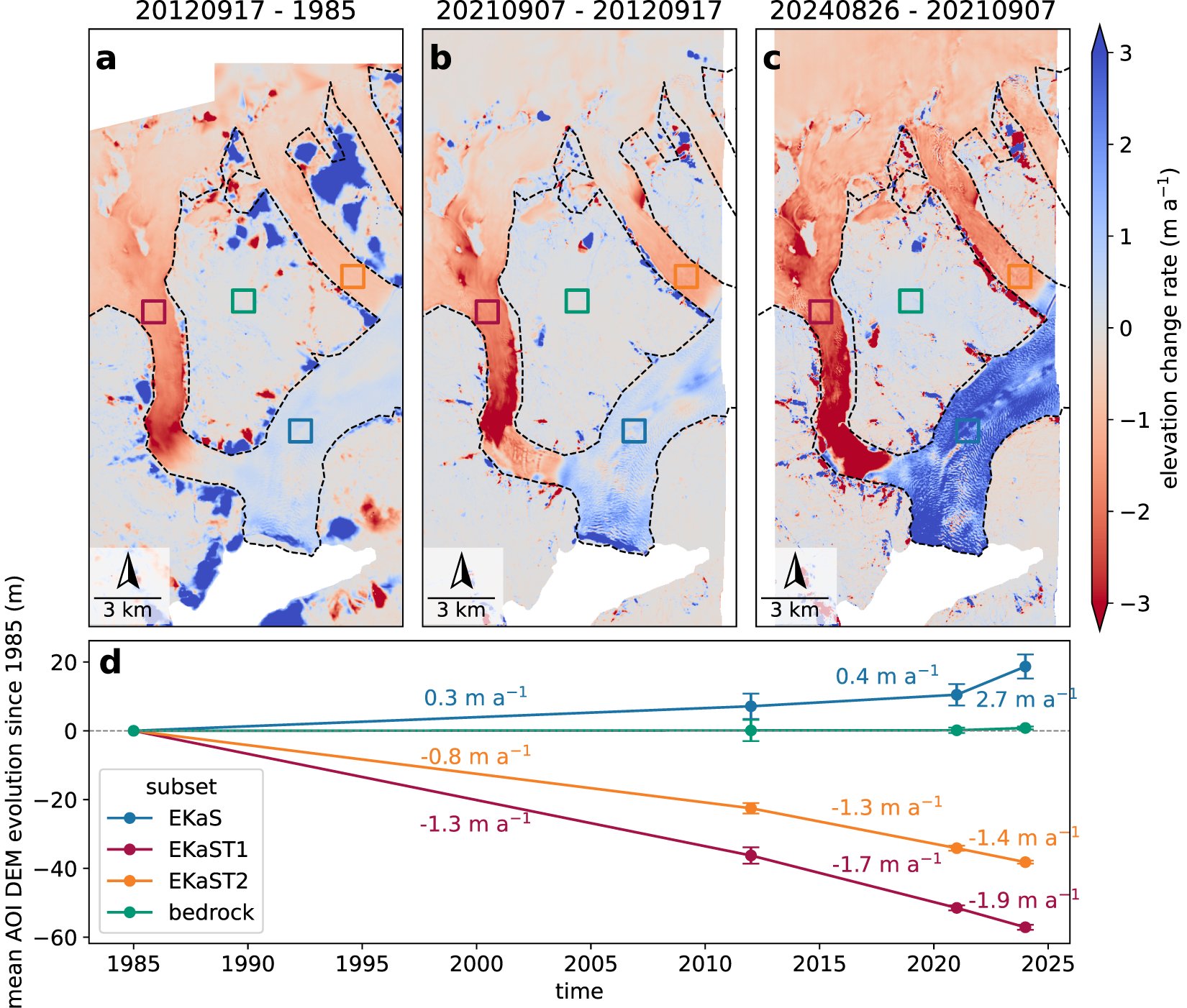

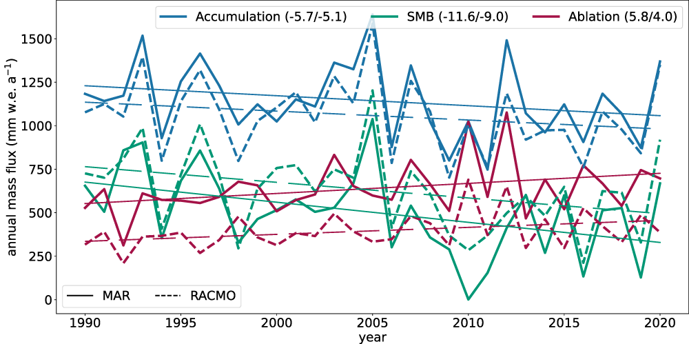

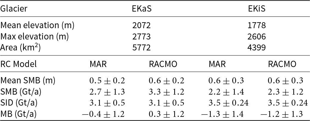


 Open access

